Linear Algebra · Preface This is an early draft of a textbook on linear algebra. There is an...
64
Linear Algebra Dave Bayer
Transcript of Linear Algebra · Preface This is an early draft of a textbook on linear algebra. There is an...
Linear Algebra
Dave Bayer

c© 2007 by Dave BayerAll rights reserved
Projective PressNew York, NY USA
http://projectivepress.com/LinearAlgebra
Dave BayerDepartment of MathematicsBarnard CollegeColumbia UniversityNew York, New York
Draft of January 12, 2007
Contents
Contents i
Preface iii
Introduction v
1 Systems of equations 1
2 Linear maps 3
3 Vector spaces 5
4 Determinants 7
5 Coordinates 9
6 Polynomials 116.1 Modular arithmetic . . . . . . . . . . . . . . . . . . . . . . . . . . . . . 126.2 Polynomial interpolation . . . . . . . . . . . . . . . . . . . . . . . . . . 206.3 Interpolation mod p(x) . . . . . . . . . . . . . . . . . . . . . . . . . . . 25
7 Functions of matrices 317.1 Polynomials and power series . . . . . . . . . . . . . . . . . . . . . . . 317.2 The characteristic polynomial . . . . . . . . . . . . . . . . . . . . . . . 367.3 Rings and fields . . . . . . . . . . . . . . . . . . . . . . . . . . . . . . . 407.4 Diagonal and triangular forms . . . . . . . . . . . . . . . . . . . . . . 437.5 The Cayley-Hamilton Theorem . . . . . . . . . . . . . . . . . . . . . . 437.6 Repeated roots . . . . . . . . . . . . . . . . . . . . . . . . . . . . . . . . 49
i

ii CONTENTS
8 Inner products 53
Index 55
Preface
This is an early draft of a textbook on linear algebra. There is an accompanyingbook, An Atlas of Matrices, giving examples suitable for working by hand. I ammaking these texts available in incomplete form for the benefit of my linear algebrastudents at Barnard College and Columbia University.
Linear algebra is a transitional subject in the mathematics curriculum. It can beone of the last math courses taken by students heading off to various applications,and these students are well served by existing textbooks that focus on applications.However, pulled in many directions by these competing interests, the algebra in lin-ear algebra has a tendency to get lost. Mathematics itself, and algebra in particular,is a great application of linear algebra.
Linear algebra is also the first semester of algebra for math majors, leading di-rectly into the modern algebra sequence. Students who haven’t picked up a fair bit ofalgebra by the time that they begin modern algebra have a tendency to hit a brickwall. I envision this book as a supplementary text for math majors who have theambition to learn as much algebra as they can, as soon as they can. For example, weuse linear algebra to study the algebra of polynomials, and then apply this theoryto better understand functions of a matrix.
This draft is currently in a very fragmented state. For now, there are variousstubs for chapters-to-be. I am completing the chapter on eigenvalues and eigen-vectors first, so that I will know exactly what material is needed to prepare for thischapter. For this reason, partial drafts of this text will not be self-contained.
This is a draft of January 12, 2007. The most recent drafts of these texts may bedownloaded from
http://projectivepress.com/LinearAlgebra
DAVE BAYER
New York, NYJanuary 2007
iii


Introduction
A matrix is a box of numbers arranged in a grid, like
A =[
2 12 3
]Linear algebra is the study of matrices. Even in its most advanced form, where onestudies linear operators on infinite-dimensional spaces with no coordinate systemin sight, one relies on intuitions built by getting really good at understanding smallmatrices that can be manipulated by hand. Such matrices are the focus of this in-troductory text. We will pile on lots of theory, but theory that is relevant to tacklingincreasingly difficult problems involving small matrices.
Matrices act by multiplication on vectors, elements of n-dimensional space, inthe same way that numbers act by multiplication on other numbers in the realline. One can think of matrices as “rich” numbers. Like computer programmersfollowing a modular design, we will alternately look inside the box of numbers tofiddle with the low-level behavior of a matrix, and close up the box to think of thematrix as a single entity. The analogy between matrices and numbers is a powerfulone; we can add and multiply matrices, solve systems of equations by multiplyingby inverse matrices, substitute matrices for variables in polynomial expressions,make matrices of matrices, and so forth. This is the spirit of algebra, accepting abroad notion as to what constitutes a value that may be manipulated in algebraicexpressions. Linear algebra is the algebra of matrices.
There is room in n dimensions for more subtle behavior than in one dimension,so the behavior of matrices can be more subtle than that of numbers. For example,in the real line there is only room to make half-turns, facing alternately in the direc-tions of ∞ and−∞. Multiplication by−1 can be thought of as a half-turn. Alreadyin the plane there is room to rotate by an arbitrary angle, and there are matrices thatrepresent each of these rotations, just as there are complex numbers that representeach of these rotations.
Three objects in a row can be permuted in more than one way, e.g. swap the twoobjects on the left, or take the object on one end and move it to the other end, slid-
v
vi INTRODUCTION
ing the other objects over. This is the simplest example of operations where ordermatters; carrying out these steps gives different results, depending on which stepcomes first. Matrices can replicate this behavior, by rearranging the order of thecoordinates in 3-dimensional space, and matrix multiplication can give differentresults, depending on which matrix comes first. We say that matrix multiplicationis noncommutative.
This again is in keeping with the spirit of algebra. Rather than hard-wiring therules of real arithmetic into our brains, we learn to flexibly flip switches to recon-figure the rules that we apply, so that we don’t automatically make simplificationsthat aren’t allowed. To work with matrices, we learn to keep track of the orderof multiplication, which is not an issue in real arithmetic. Why always play chesswhen there are other games? The appeal of algebra is the appeal of learning newgames. For all its complexity, matrix arithmetic is far more interesting than realarithmetic.
The complexity of matrices is the complexity of the real world. It makes a dif-ference whether one cracks an egg before frying it, or fries it in its shell and cracksit later. Such is a matter of taste, but the order matters. More tragically, one candrink a glass of wine and then drop the glass, but not easily the other way around.Order matters in a vast array of applications which can be modeled by matrices,but not by numbers. Not only can we think of matrices as numbers, we can thinkof matrices as actions. For example, we will first learn to solve systems of linearequations by rescaling, adding, and swapping around the equations. Then, we willstore these actions as matrices, with the property that multiplying by the matrixcarries out the action. This is a common mode of thought in linear algebra. Whenwe say a matrix acts on a space, we mean this quite literally.
Historically, the study of matrices began with the study of solutions to linearsystems of equations. Only later was the subject generalized to the study of linearmaps, functions with a property exemplified by matrices. We approach each of thesepoints of view on an equal footing; the first two chapters can be read independentlyof each other.
Chapter 1
Systems of equations
Lorem ipsum dolor sit amet, consectetur adipisicing elit, sed do eiusmod temporincididunt ut labore et dolore magna aliqua. Ut enim ad minim veniam, quis nos-trud exercitation ullamco laboris nisi ut aliquip ex ea commodo consequat. Duisaute irure dolor in reprehenderit in voluptate velit esse cillum dolore eu fugiatnulla pariatur. Excepteur sint occaecat cupidatat non proident, sunt in culpa quiofficia deserunt mollit anim id est laborum.

Chapter 2
Linear maps
Lorem ipsum dolor sit amet, consectetur adipisicing elit, sed do eiusmod temporincididunt ut labore et dolore magna aliqua. Ut enim ad minim veniam, quis nos-trud exercitation ullamco laboris nisi ut aliquip ex ea commodo consequat. Duisaute irure dolor in reprehenderit in voluptate velit esse cillum dolore eu fugiatnulla pariatur. Excepteur sint occaecat cupidatat non proident, sunt in culpa quiofficia deserunt mollit anim id est laborum.


Chapter 3
Vector spaces
Lorem ipsum dolor sit amet, consectetur adipisicing elit, sed do eiusmod temporincididunt ut labore et dolore magna aliqua. Ut enim ad minim veniam, quis nos-trud exercitation ullamco laboris nisi ut aliquip ex ea commodo consequat. Duisaute irure dolor in reprehenderit in voluptate velit esse cillum dolore eu fugiatnulla pariatur. Excepteur sint occaecat cupidatat non proident, sunt in culpa quiofficia deserunt mollit anim id est laborum.

C
M
Y
CM
MY
CY
CMY
K
P4.pdf 12/25/06 7:20:50 PMP4.pdf 12/25/06 7:20:50 PM
Chapter 4
Determinants
The determinant is an expression in the entries of a square matrix, that appearsthroughout linear algebra. If it didn’t already come with hundreds of years of his-tory and a myriad of interpretations, the attentive student would notice the deter-minant as a pattern cropping up all over the place, and give it a name. For us, thedeterminant is first and foremost a formula, whose pattern we want to understand.Then we will consider interpretations of this formula.
For an operational definition, the determinant of a matrix is the number thatmost closely resembles the matrix. Matrices are capable of far more subtle behaviorthan numbers, such as representing actions where the order of operations matters,so it is too much to ask that there be a number that exactly reflects the propertiesof a matrix. If this were possible, then we wouldn’t need matrices. Nevertheless,it is reasonable to ask that an invertible matrix be represented by an invertiblenumber, for the product of two matrices to be represented by the product of theircorresponding numbers, and so forth. The determinant is that number.

Chapter 5
Coordinates
Lorem ipsum dolor sit amet, consectetur adipisicing elit, sed do eiusmod temporincididunt ut labore et dolore magna aliqua. Ut enim ad minim veniam, quis nos-trud exercitation ullamco laboris nisi ut aliquip ex ea commodo consequat. Duisaute irure dolor in reprehenderit in voluptate velit esse cillum dolore eu fugiatnulla pariatur. Excepteur sint occaecat cupidatat non proident, sunt in culpa quiofficia deserunt mollit anim id est laborum.

Chapter 6
Polynomials
There are striking parallels between the algebra of matrices and the algebra of poly-nomials. To prepare for the theory of functions of a matrix, we review some poly-nomial algebra.
If one steps back and takes a fresh look at polynomials, they now look verymuch a part of linear algebra. A polynomial in the variable x is after all a linearcombination of powers of x. This is a useful point of view. If we take all powersof some object x in an arbitrary algebraic setting over a field F, either the powersare linearly independent, spanning an infinite dimensional subspace, or they arelinearly dependent, and we can write the first dependent power
xd = cd−1xd−1 + . . . + c1x1 + c0
as a linear combination of the preceding powers. This rule can then be used repeat-edly to rewrite any higher power of x in terms of {xd−1, . . . , x, 1}, showing that thisset is a basis for all powers of x. In this case, x behaves as if we are working modulothe polynomial
p(x) = xd − cd−1xd−1 − . . . − c1x1 − c0
Square matrices are such a setting. The space of all n× n matrices over a fieldF is an n2-dimensional vector space, so it isn’t possible for all powers of an n× nmatrix A to be linearly independent of each other. There simply isn’t enough room.It must be the case that for some d ≤ n2,
Ad = cd−1Ad−1 + . . . + c1A1 + c0I
In other words, it is inevitable that square matrices behave as if we are workingmodulo some polynomial, because their powers live in a finite dimensional vectorspace.
12 Polynomials
We are very interested in understanding such polynomials. It turns out thatthe least such d is smaller than this argument suggests; we can always find such adependence with d ≤ n. Viewing A as a linear map V → V, it is the dimension n ofV, not the dimension n2 of possible matrices, that matters. Still, this first argumentmakes it clear that there must be some such polynomial, hence our interest now inpolynomials.
6.1 Modular arithmetic
Integers
Let m be an integer. Two integers a, b are equivalent mod m if their difference a− bis a multiple of m. We write
a ≡ b mod m
and say that we are computing in the ring Z/mZ of integers mod m. For example,8 ≡ 2 mod 3, because 8− 2 = 6 is a multiple of 3. The distinct elements of Z/3Zare {0, 1, 2}, which are the possible remainders under division by 3.
It is a tremendous simplification to be able to work modulo an integer m; ourcalculations can take place in the finite set {0, 1, . . . , m − 1} of remainders underdivision by m. This can mean the difference between a value fitting in one word ofmemory on a computer, and a value not fitting on the computer at all.
Example 6.1. The integer 21024 is a 309 digit number, but 21024 mod 5 can be com-puted by repeated squaring mod 5; after the second squaring, the value becomesand stays 1:
22 ≡ 4 mod 524 ≡ (22)2 ≡ 1 mod 5
. . . 21024 ≡ (2512)2 ≡ 1 mod 5
Polynomials
One can also work with polynomials modulo a polynomial p(x). Computationally,this is again a tremendous simplification; our calculations can all take place in thefinite dimensional vector space of remainders under division by p.
Two polynomials f , g are equivalent mod p if their difference f − g is a multipleof p. We again write
f (x) ≡ g(x) mod p(x)
and say that we are computing in the ring F[x]/p(x)F[x] of polynomials mod p.In this notation, F[x] stands for the ring of all polynomials in the variable x withcoefficients in our field F.
6.1. Modular arithmetic 13
Example 6.2. Let p(x) = x2 + 1. We have
x2 ≡ −1 mod x2 + 1
because x2− (−1) = x2 + 1. The distinct elements of R[x]/(x2 + 1)R[x] are now allpossible remainders under division by x2 + 1. This is a 2-dimensional vector spaceover R with basis {1, x}.
The complex numbers
The complex numbers C can be viewed as an example of polynomial modulararithmetic.
Example 6.2 looks familiar. The complex numbers C are also a 2-dimensionalvector space over R, with basis {1, i}, and i2 = −1. The complex numbers look likeR[x]/(x2 + 1)R[x], only with x replaced by i. They are an important special case ofworking modulo a polynomial, with x getting the special name i.
Viewing C as the vector space R2, we can represent multiplication by i as a 2× 2matrix A. Multiplication by i maps the basis {1, i} to {i,−1}, so in vector notationwe want A(1, 0) = (0, 1) and A(0, 1) = (−1, 0). This is the matrix
A =[
0 −11 0
]which we recognize as a rotation by π/2. Indeed, multiplication by i rotates thecomplex plane by π/2. For all intents and purposes, this matrix A is the imaginarynumber i. The matrix A goes with the notation R2, the variable x goes with thenotation R[x]/(x2 + 1)R[x], and i goes with the notation C, but they are all thesame thing.
If A and i are the same thing, what about i2 + 1 = 0? We have
A2 + I =[
0 −11 0
]2
+[
1 00 1
]=
[−1 0
0 −1
]+
[1 00 1
]= 0
A acts just like i, so this is no surprise. We now have three views of the complexnumbers: C, and R[x]/(x2 + 1)R[x], and the ring of all polynomial expressionsin A. For example, the complex number 2− 3i can be viewed as the polynomial2− 3x mod x2 + 1, and as the matrix expression 2I− 3A.
For an arbitrary square matrix A, the ring of all polynomial expressions in Ais not so different. The governing equation x2 + 1 = 0 changes, but the idea is thesame. C is just a special case, with its own notation.
14 Polynomials
The dual numbers
A closely related example is the ring of dual numbers, modeled after the idea ofan infinitesimal in calculus. In calculus, ε is taken to be so small that ε2 is effec-tively zero. In algebra, we simply dictate that ε2 = 0 by working modulo ε2. In thenotation of modular arithmetic, we have
ε2 ≡ 0 mod ε2
We are again working modulo a polynomial, with our variable getting the specialname ε. The ring of dual numbers can be denoted R[ε]/ε2R[ε].
Not surprisingly given its origins, this ε can be used to differentiate algebraicexpressions. If f (x) is a polynomial or power series, then
f (a +ε) ≡ f (a) + f ′(a)ε mod ε2 (6.1)
This is just a version of the familiar equation
f ′(a) = limε→0
f (a +ε)− f (a)ε
In calculus, a limit is required to suppress the effects ofε2. Here, no limit is requiredbecause we are working modulo ε2.
When we are firmly ensconced in this setting, we will drop the notation ≡ infavor of = and stop writing “mod ε2” after every equation.
Example 6.3. If f (x) = x3 then working modulo ε2,
f (1 +ε) = (1 +ε)3 = 1 + 3ε + 3ε2 +ε3 = 1 + 3ε
This agrees with f ′(1) = 3.
The dual numbers are a 2-dimensional vector space over R with basis {ε, 1}.Viewing the dual numbers as the vector space R2, we can represent multiplicationby ε as a 2× 2 matrix N. Multiplication by ε maps the basis {ε, 1} to {0,ε}, so invector notation we want N(1, 0) = (0, 0) and N(0, 1) = (1, 0). This is the matrix
N =[
0 10 0
]This matrix is the simplest example of a nilpotent matrix:
Definition 6.4. A square matrix N is nilpotent if some power of N is the zero matrix.
Here we have N2 = 0, mirroring the fact that ε2 = 0. We can view the dualnumbers as the ring of all polynomial expressions in N.
6.1. Modular arithmetic 15
Example 6.5. If the matrix N acts exactly like ε, then we should be able to differen-tiate using N. Indeed, again taking f (x) = x3,
f (I + N) =([
1 00 1
]+
[0 10 0
])3
=[
1 00 1
]+ 3
[0 10 0
]= f (1) I + f ′(1) N
This calculation agrees with that of example 6.3, with ε replaced by N.
In general, equation 6.1 takes the matrix form
f (aI + N) = f (a) I + f ′(a) N (6.2)
where N is any nilpotent matrix that acts like ε. In other words, N can be anysquare matrix with N2 = 0.
Rational canonical form
In both of the preceding examples, we could view the ring of polynomials modulop(x) as a 2-dimensional vector space with basis {x, 1}. In both of these rings, x2 wasa linear combination of these basis elements, allowing us to reduce higher powersof x to an expression in x and 1.
In general, when p(x) is a polynomial of degree n, the distinct elements ofF[x]/p(x)F[x] are the possible remainders under division by p. Our ring is nowan n-dimensional vector space with basis {xn−1, . . . , x, 1}. In this ring, xn is a linearcombination of these basis elements, allowing us to reduce higher powers of x toan expression in xn−1, . . . , x, 1. For some coefficients cn−1, . . . , c1, c0 we have
xn ≡ cn−1xn−1 + . . . + c1x1 + c0 mod p(x)
This would not change if we replace p by any nonzero multiple of itself, so wemight as well take p to be the monic polynomial
p(x) = xn − cn−1 xn−1 − . . . − c1 x − c0
We can represent multiplication by x as an n× n matrix A. Multiplication by xmaps the basis {xn−1, . . . , x, 1} to
{ cn−1xn−1 + . . . + c1x + c0, xn−1, . . . , x }
16 Polynomials
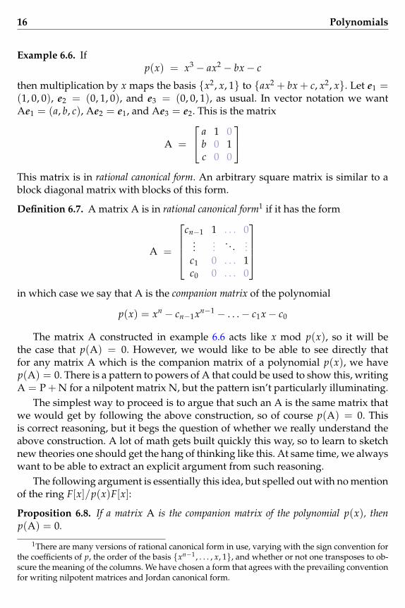
Example 6.6. Ifp(x) = x3 − ax2 − bx− c
then multiplication by x maps the basis {x2, x, 1} to {ax2 + bx + c, x2, x}. Let e1 =(1, 0, 0), e2 = (0, 1, 0), and e3 = (0, 0, 1), as usual. In vector notation we wantAe1 = (a, b, c), Ae2 = e1, and Ae3 = e2. This is the matrix
A =
a 1 0b 0 1c 0 0
This matrix is in rational canonical form. An arbitrary square matrix is similar to ablock diagonal matrix with blocks of this form.
Definition 6.7. A matrix A is in rational canonical form1 if it has the form
A =
cn−1 1 . . . 0
......
. . ....
c1 0 . . . 1c0 0 . . . 0
in which case we say that A is the companion matrix of the polynomial
p(x) = xn − cn−1xn−1 − . . .− c1x− c0
The matrix A constructed in example 6.6 acts like x mod p(x), so it will bethe case that p(A) = 0. However, we would like to be able to see directly thatfor any matrix A which is the companion matrix of a polynomial p(x), we havep(A) = 0. There is a pattern to powers of A that could be used to show this, writingA = P + N for a nilpotent matrix N, but the pattern isn’t particularly illuminating.
The simplest way to proceed is to argue that such an A is the same matrix thatwe would get by following the above construction, so of course p(A) = 0. Thisis correct reasoning, but it begs the question of whether we really understand theabove construction. A lot of math gets built quickly this way, so to learn to sketchnew theories one should get the hang of thinking like this. At same time, we alwayswant to be able to extract an explicit argument from such reasoning.
The following argument is essentially this idea, but spelled out with no mentionof the ring F[x]/p(x)F[x]:
Proposition 6.8. If a matrix A is the companion matrix of the polynomial p(x), thenp(A) = 0.
1There are many versions of rational canonical form in use, varying with the sign convention forthe coefficients of p, the order of the basis {xn−1 , . . . , x, 1}, and whether or not one transposes to ob-scure the meaning of the columns. We have chosen a form that agrees with the prevailing conventionfor writing nilpotent matrices and Jordan canonical form.
6.1. Modular arithmetic 17
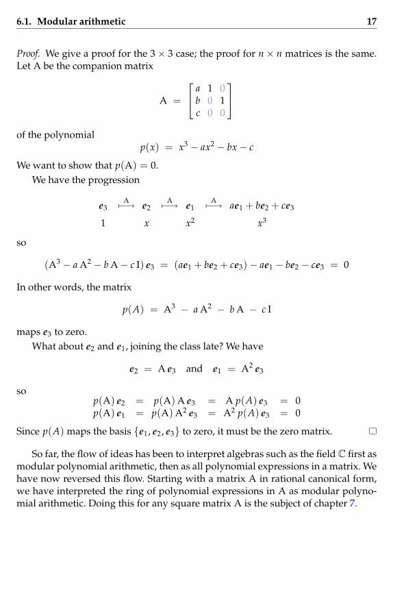
Proof. We give a proof for the 3× 3 case; the proof for n× n matrices is the same.Let A be the companion matrix
A =
a 1 0b 0 1c 0 0
of the polynomial
p(x) = x3 − ax2 − bx− c
We want to show that p(A) = 0.We have the progression
e3A7−→ e2
A7−→ e1A7−→ ae1 + be2 + ce3
1 x x2 x3
so
(A3 − a A2 − b A− c I) e3 = (ae1 + be2 + ce3)− ae1 − be2 − ce3 = 0
In other words, the matrix
p(A) = A3 − a A2 − b A − c I
maps e3 to zero.What about e2 and e1, joining the class late? We have
e2 = A e3 and e1 = A2 e3
sop(A) e2 = p(A) A e3 = A p(A) e3 = 0p(A) e1 = p(A) A2 e3 = A2 p(A) e3 = 0
Since p(A) maps the basis {e1, e2, e3} to zero, it must be the zero matrix.
So far, the flow of ideas has been to interpret algebras such as the field C first asmodular polynomial arithmetic, then as all polynomial expressions in a matrix. Wehave now reversed this flow. Starting with a matrix A in rational canonical form,we have interpreted the ring of polynomial expressions in A as modular polyno-mial arithmetic. Doing this for any square matrix A is the subject of chapter 7.
18 Polynomials
A geometric interpretation
When a polynomial p factors into distinct linear factors, there is a close connectionbetween arithmetic mod p(x) and the set of roots of p. Namely, a polynomial isequivalent to zero mod p(x) if and only if it vanishes on the roots of p. It followsthat two polynomials are equivalent mod p(x) if and only if they have the samevalues on the roots of p.
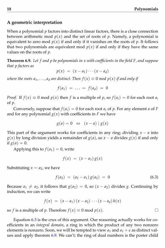
Theorem 6.9. Let f and p be polynomials in x with coefficients in the field F, and supposethat p factors as
p(x) = (x− a1) · · · (x− ad)
where the roots a1, . . . , ad are distinct. Then f (x) ≡ 0 mod p(x) if and only if
f (a1) = . . . = f (ad) = 0
Proof. If f (x) ≡ 0 mod p(x) then f is a multiple of p, so f (ai) = 0 for each root aiof p.
Conversely, suppose that f (ai) = 0 for each root ai of p. For any element a of Fand for any polynomial g(x) with coefficients in F we have
g(a) = 0 ⇔ (x− a) | g(x)
This part of the argument works for coefficients in any ring; dividing x − a intog(x) by long division yields a remainder of g(a), so x− a divides g(x) if and onlyif g(a) = 0.
Applying this to f (a1) = 0, write
f (x) = (x− a1) g(x)
Substituting x = a2, we have
f (a2) = (a2 − a1) g(a2) = 0 (6.3)
Because a1 6= a2, it follows that g(a2) = 0, so (x − a2) divides g. Continuing byinduction, we can write
f (x) = (x− a1) (x− a2) · · · (x− ad) h(x)
so f is a multiple of p. Therefore f (x) ≡ 0 mod p(x).
Equation 6.3 is the crux of this argument. Our reasoning actually works for co-efficients in an integral domain, a ring in which the product of any two nonzeroelements is nonzero. Soon, we will be tempted to view a1 and a1 +ε as distinct val-ues and apply theorem 6.9. We can’t; the ring of dual numbers is the poster child
6.1. Modular arithmetic 19
for a ring that isn’t an integral domain, because ε is nonzero but ε2 is zero. How-ever, the spirit of this idea points us in the right direction. What we can do insteadis to consider the coefficient of ε in various dual number expressions, analogous toconsidering the imaginary part of a complex number.
Working mod p(x) is adopting the stance that the domain of our polynomials isthe set of roots of p. We’re taking p itself to be zero because p is zero on these roots.Two polynomials g and h may disagree on some elements of R other than theseroots, but we’re adopting the stance that we don’t care about any other elements ofR. As long as g and h are the same function when restricted to the roots of p, to usthey are the same function.
This point of view is the beginning of a subject called algebraic geometry. There,one studies systems of polynomial equations in many variables, both in terms ofthe geometry of the solution sets, and in terms of the algebra modulo the defin-ing equations. Again, this is taking the stance that the solution sets are the do-mains of the polynomials, as if all other points don’t even exist. This turns out tobe a powerful idea. Around the same time that painting went abstract, so did alge-braic geometry. Somebody flipped a switch, and suddenly all of the ambient spaceswere gone, leaving just bare point sets, curves and surfaces to study by themselves.We’re flipping this switch by working modulo p(x).
When two roots of p come together, say a1 and a2, theorem 6.9 requires modifi-cation. The condition f (a1) = 0 insures that x− a1 divides f , but it is not enough toinsure that (x− a1)2 divides f . It takes d conditions to determine whether f (x) ≡ 0mod p(x). When a1 and a2 come together, we have lost a condition, which we re-cover as the condition f ′(a1) = 0.
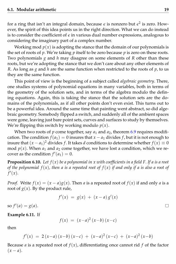
Proposition 6.10. Let f (x) be a polynomial in x with coefficients in a field F. If a is a rootof the polynomial f (x), then a is a repeated root of f (x) if and only if a is also a root off ′(x).
Proof. Write f (x) = (x− a)g(x). Then a is a repeated root of f (x) if and only a is aroot of g(x). By the product rule,
f ′(x) = g(x) + (x− a) g′(x)
so f ′(a) = g(a).
Example 6.11. Iff (x) = (x−a)2 (x−b) (x−c)
then
f ′(x) = 2 (x−a) (x−b) (x−c) + (x−a)2 (x−c) + (x−a)2 (x−b)
Because a is a repeated root of f (x), differentiating once cannot rid f of the factor(x− a).
20 Polynomials
This pattern reappears throughout this chapter. Working over the field R,knowing f (a1) and f ′(a1) is pretty much the same information as knowing f (a1)and f (a2) when a1 and a2 are close; we can use f ′(a1) to estimate f (a2). However,this pattern holds for any field, including fields where we cannot reason analyti-cally. We can work with an arbitrary field F by using the ring of dual numbers.
Proposition 6.12. Let f and p be polynomials in x with coefficients in the field F, andsuppose that p factors as
p(x) = (x− a1)2 (x− a3) · · · (x− ad)
where the roots a1, a3, . . . , ad are distinct. Then f (x) ≡ 0 mod p(x) if and only if
f (a1) = f ′(a1) = f (a3) = . . . = f (ad) = 0 (6.4)
Proof. If f (x) ≡ 0 mod p(x), then f is a multiple of p. We work with the values
a1, a1 +ε, a3, . . . , ad (6.5)
Note that working modulo ε2,
p(a1 +ε) = ε2 (a1 +ε− a3) · · · (a1 +ε− ad) = 0
Therefore p(x) vanishes on each of the values 6.5, so we have
f (a1) = f (a1 +ε) = f (a3) = . . . = f (ad) = 0
Since f (a1 +ε) = f (a1) +ε f ′(a1), we get the condition f ′(a1) = 0.Conversely, suppose that the conditions 6.4 hold. From f (a1) = f ′(a1) = 0 we
get f (a1 +ε) = 0. Writef (x) = (x− a1) g(x)
where g is the quotient of f under division by x− a1. Then
f (a1 +ε) = (a1 +ε− a1) g(a1 +ε) = ε (g(a1) +ε g′(a1)) = ε g(a1) = 0
This is identically zero as an expression in the ring of dual numbers, so the coeffi-cient g(a1) of ε must be zero. Therefore, x− a1 divides g(x), so x− a1 divides f (x)twice. It follows that f is a multiple of p, so f (x) ≡ 0 mod p(x).
We could have instead used proposition 6.10 here. We applied the ring of dualnumbers to illustrate their use; they will appear again.
6.2 Polynomial interpolation
A polynomial of degree < d is determined by its values at d distinct points. There isa steep, direct assault on this statement using the Vandermonde matrix, and a cleverway to sidestep its complexity using Lagrange interpolation.

6.2. Polynomial interpolation 21
The Vandermonde matrix
Proposition 6.13. Let a1, . . . , ad be distinct values in the field F. There is a unique poly-nomial of degree < d
f (x) = cd−1xd−1 + . . . + c1x + c0
determined by the values f (a1), . . . , f (ad).
Proof. The coefficients of f (x) are determined by the system of equations
ad−11 ad−2
1 . . . a1 1
ad−12 ad−2
2 . . . a2 1...
......
...
ad−1d−1 ad−2
d−1 . . . ad−1 1
ad−1d ad−2
d . . . ad 1
cd−1
cd−2
...
c1
c0
=
f (a1)
f (a2)...
f (ad−1)
f (ad)
(6.6)
where the ith row is the equation
cd−1 ad−1i + cd−2 ad−2
i + . . . + c1 ai + c0 = f (ai)
Let A denote the coefficient matrix of this system of equations. A matrix of thisform is called a Vandermonde matrix. We will show that A has the determinant
det(A) = ∏i< j
(ai − a j) (6.7)
It follows that this system of equations has a unique solution whenever each ai −a j 6= 0.
It is a worthy exercise to deduce equation 6.7 directly by induction. However,there is also an argument using modular arithmetic. Let g be the polynomial givenby the right hand side of equation 6.7, where we take a1, . . . , ad to be variables:
g(a1, . . . , ad) = ∏i< j
(ai − a j)
Consider the term of g obtained by taking the product of the first variables in eachfactor,
g(a1, . . . , ad) = ad−11 ad−2
2 · · · ad−1 + . . .
We recognize this term as the product of the diagonal entries of A, so it is also aterm of det(A), viewed as a polynomial in a1, . . . , ad:
det(A) = ad−11 ad−2
2 · · · ad−1 + . . .
22 Polynomials
The polynomials g and det(A) are each homogeneous of degree(d2
)= (d− 1) + (d− 2) + . . . + 1
so if g divides det(A), they must be the same polynomial.We now work modulo ai − a j. If we substitute ai = a j in the matrix A, then the
ith and jth rows of A become the same, so
det(A) ≡ 0 mod ai − a j
Therefore det(A) is a multiple of ai − a j for each i < j, so g divides det(A).
Example 6.14. Let d = 3, and let a, b, c be values in F. Then
A =
a2 a 1b2 b 1c2 c 1
and
(a− b)(a− c)(b− c) = a2b + b2c + ac2 − a2c− ab2 − bc2 = det(A)
Notice that of the eight possible terms in this product, two are abc− abc, leavingthe six shown.
When two points come together, say a1 and a2, the determinant of A vanishesand we can no longer solve for the polynomial f using the system of equations6.6. In other words, f is no longer determined by its values at a1, a2, . . . , ad becausethe value at a1 = a2 is only useful once; we need another value. However, thepolynomial f is determined by these values and the derivative f ′(a1).
To find the polynomial f (x) determined by the values
f (a1), f ′(a1), f (a3), . . . , f (ad) (6.8)
we want to solve the system of equationsad−1
1 . . . a21 a1 1
(d−1)ad−21 . . . 2a1 1 0
ad−13 . . . a2
3 a3 1...
......
ad−1d . . . a2
d ad 1
cd−1
...c2c1c0
=
f (a1)f ′(a1)f (a3)
...f (ad)
(6.9)
where the second row is the equation
(d− 1) cd−1 ad−21 + . . . + 2 c2 a1 + c1 = f ′(a1)
6.2. Polynomial interpolation 23
We can use dual numbers to understand this matrix. Working modulo ε2, wecan transform 6.6 into 6.9 by substituting a2 = a1 +ε, applying equation 6.1, sub-tracting the first row from the second, and factoring out an ε from the second row.
Making this same substitution into g yields
g(a1, a1 +ε, a3, . . . , ad) = ε∂g∂a2
(a1, a1, a3, . . . , ad)
because g(a1, a1, a3, . . . , ad) vanishes. Writing this out, we have
∏i< j
(ai − a j) = (a1 − (a1 +ε))d
∏j=3
(a1 − a j)((a1 +ε)− a j) ∏3≤i< j≤d
(ai − a j)
= −εd
∏j=3
(a1 − a j)2∏
3≤i< j≤d(ai − a j)
Making this substitution into det(A) yields∣∣∣∣∣∣∣∣∣∣∣∣∣∣
ad−11 . . . a2
1 a1 1
(a1+ε)d−1 . . . (a1+ε)2 a1+ε 1
ad−13 . . . a2
3 a3 1...
......
...
ad−1d . . . a2
d ad 1
∣∣∣∣∣∣∣∣∣∣∣∣∣∣= ε
∣∣∣∣∣∣∣∣∣∣∣∣∣∣
ad−11 . . . a2
1 a1 1
(d−1)ad−21 . . . 2a1 1 0
ad−13 . . . a2
3 a3 1...
......
...
ad−1d . . . a2
d ad 1
∣∣∣∣∣∣∣∣∣∣∣∣∣∣following the same steps that transform 6.6 into 6.9.
Comparing these equivalences, we see that the determinant of the system ofequations 6.9 is nonzero whenever a1, a3, . . . , ad are distinct values, so the polyno-mial f (x) is uniquely determined by the values 6.8. The general case follows thesame pattern.
We could be forgiven for expecting proposition 6.13 to be useless in the situa-tion where the value a1 repeats. However, the ring of dual numbers provides uswith a device for viewing the repeated value a1 as the two distinct values a1 anda1 +ε, allowing us to apply proposition 6.13 after all. Intuitively, the two values a1and a1 +ε are right next to each other, differing infinitesimally by ε. We have re-placed differentiation with algebra2. In algebraic geometry, one generalizes this ideato model multiplicities of higher dimensional sets, as an algebraic counterpart tomultivariable calculus.
We will see a version of this phenomenon in chapter 7. Ordinarily, a functionapplied to a matrix is determined by its values at the eigenvalues of the matrix. How-ever, when two eigenvalues come together, we also need to consider the derivativeat the repeated eigenvalue. This is parallel to polynomial interpolation; our decom-position of the matrix will sprout a nilpotent matrix playing the role of ε here.
2Few mathematicians see this as an even trade, but there are plenty of takers on both sides.
24 Polynomials
Lagrange interpolation
The complexity of the Vandermonde matrix is due to the fact that while
{xd−1, xd−2, . . . , x, 1}
may be the obvious choice of a basis for the polynomials of degree < d, it is poorlyadapted to the problem of interpolating polynomials from their values. We wouldbe much happier if the Vandermonde matrix were a diagonal matrix, but it isn’t.
The idea of Lagrange interpolation is to choose a basis for the polynomials ofdegree < d that diagonalizes the problem of interpolating polynomials from theirvalues. Indeed, the method is so simple that none of these big words are necessary;one can apply this method knowing next to nothing3. The virtue of understandingLagrange interpolation in the language of linear algebra is that it represents a com-mon pattern we want to reapply. Whenever possible, it pays to find a basis thatdiagonalizes the problem one is studying.
Example 6.15. Let f (x) be the degree two polynomial determined by the valuesf (a), f (b), and f (c). Then
f (x) = f (a)(x− b)(x− c)(a− b)(a− c)
+ f (b)(x− a)(x− c)(b− a)(b− c)
+ f (c)(x− a)(x− b)(c− a)(c− b)
It is clear by inspection that this expression yields the desired values; substitutingx = a, b or c, all but one quotient vanishes, and the remaining quotient cancels outto 1. We have expressed the polynomial f (x) in Lagrange form.
Conceptually, we have chosen the basis
g1(x) =(x− b)(x− c)(a− b)(a− c)
, g2(x) =(x− a)(x− c)(b− a)(b− c)
, g3(x) =(x− a)(x− b)(c− a)(c− b)
for the space of polynomials of degree < 3. Now, any such polynomial can beexpressed as a linear combination of g1, g2, and g3. We want to solve for r1, r2, andr3 in the system of equations
r1 g1(a) + r2 g2(a) + r3 g3(a) = f (a)r1 g1(b) + r2 g2(b) + r3 g3(b) = f (b)r1 g1(c) + r2 g2(c) + r3 g3(c) = f (c)
3I remember thinking of Lagrange interpolation in high school, only to be gently scolded by myteacher that this was not a new idea. While some math students worry about when they will start todo original work, one generally starts to think of new ideas long after the distinction stops mattering.It is simply fun to think of things for oneself.
6.3. Interpolation mod p(x) 25
However, this leads to the matrix equation1 0 00 1 00 0 1
r1r2r3
=
f (a)f (b)f (c)
from which we can simply read off the solution.
6.3 Interpolation mod p(x)
Suppose that the polynomial p(x) factors into the linear factors
p(x) = (x− a1) · · · (x− ad)
for distinct roots a1, . . . , ad, and that we are working modulo p(x). Then all of theresults of this chapter are applicable. This is the setting that most closely resemblesworking with a diagonalizable matrix A.
Now, any polynomial f (x) is equivalent mod p(x) to a polynomial of degree< d, so any polynomial f (x) can be interpolated from its values f (a1), . . . , f (ad).
Example 6.16. Letp(x) = (x− 2)(x− 3)(x− 4)
Then f (x) = xk can be interpolated mod p(x) from its values at the roots 2, 3, and4. By Lagrange interpolation,
xk ≡ 2k (x−3)(x−4)(2−3)(2−4)
+ 3k (x−2)(x−4)(3−2)(3−4)
+ 4k (x−2)(x−3)(4−2)(4−3)
mod p(x)
This polynomial is the unique degree < 3 polynomial determined by the valuesf (2) = 2k, f (3) = 3k, and f (4) = 4k. On the other hand, f is equivalent mod p toits remainder under division by p, which is a polynomial of degree < 3. Therefore,f (x) is this polynomial.
Recall the geometric interpretation of polynomial modular arithmetic. In theabove example, only the values 2, 3, and 4 matter. Working mod p(x), our domainis the set {2, 3, 4}, as if the rest of our field F isn’t even there. As soon as we havefound a function that agrees with f on this domain, we have found f .
In fact, the distinction between polynomials and other functions breaks downwhen our domain is a finite set; any function is equivalent mod p(x) to a polyno-mial of degree < d, which can be found by Lagrange interpolation from its valueson the roots of p.
In particular, f can be a function of several variables, where the domain of oneof the variables is the set of roots of p.
26 Polynomials
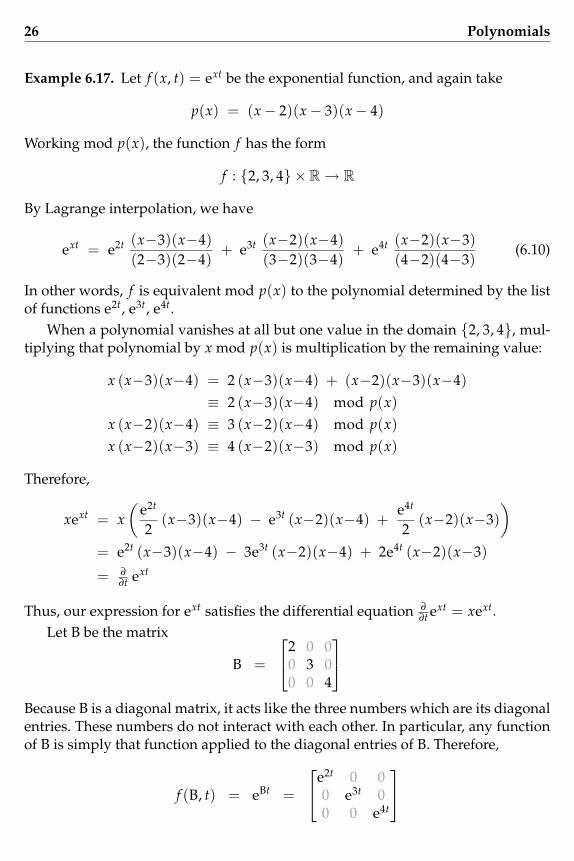
Example 6.17. Let f (x, t) = ext be the exponential function, and again take
p(x) = (x− 2)(x− 3)(x− 4)
Working mod p(x), the function f has the form
f : {2, 3, 4} ×R→ R
By Lagrange interpolation, we have
ext = e2t (x−3)(x−4)(2−3)(2−4)
+ e3t (x−2)(x−4)(3−2)(3−4)
+ e4t (x−2)(x−3)(4−2)(4−3)
(6.10)
In other words, f is equivalent mod p(x) to the polynomial determined by the listof functions e2t, e3t, e4t.
When a polynomial vanishes at all but one value in the domain {2, 3, 4}, mul-tiplying that polynomial by x mod p(x) is multiplication by the remaining value:
x (x−3)(x−4) = 2 (x−3)(x−4) + (x−2)(x−3)(x−4)≡ 2 (x−3)(x−4) mod p(x)
x (x−2)(x−4) ≡ 3 (x−2)(x−4) mod p(x)x (x−2)(x−3) ≡ 4 (x−2)(x−3) mod p(x)
Therefore,
xext = x(
e2t
2(x−3)(x−4) − e3t (x−2)(x−4) +
e4t
2(x−2)(x−3)
)= e2t (x−3)(x−4) − 3e3t (x−2)(x−4) + 2e4t (x−2)(x−3)
= ∂
∂t ext
Thus, our expression for ext satisfies the differential equation ∂
∂t ext = xext.Let B be the matrix
B =
2 0 00 3 00 0 4
Because B is a diagonal matrix, it acts like the three numbers which are its diagonalentries. These numbers do not interact with each other. In particular, any functionof B is simply that function applied to the diagonal entries of B. Therefore,
f (B, t) = eBt =
e2t 0 00 e3t 00 0 e4t
6.3. Interpolation mod p(x) 27
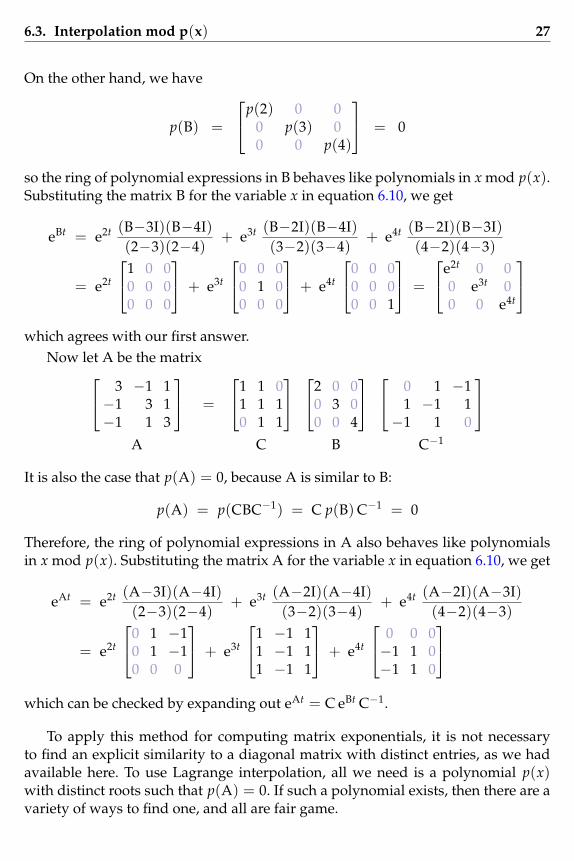
On the other hand, we have
p(B) =
p(2) 0 00 p(3) 00 0 p(4)
= 0
so the ring of polynomial expressions in B behaves like polynomials in x mod p(x).Substituting the matrix B for the variable x in equation 6.10, we get
eBt = e2t (B−3I)(B−4I)(2−3)(2−4)
+ e3t (B−2I)(B−4I)(3−2)(3−4)
+ e4t (B−2I)(B−3I)(4−2)(4−3)
= e2t
1 0 00 0 00 0 0
+ e3t
0 0 00 1 00 0 0
+ e4t
0 0 00 0 00 0 1
=
e2t 0 00 e3t 00 0 e4t
which agrees with our first answer.
Now let A be the matrix 3 −1 1−1 3 1−1 1 3
=
1 1 01 1 10 1 1
2 0 00 3 00 0 4
0 1 −11 −1 1−1 1 0
A C B C−1
It is also the case that p(A) = 0, because A is similar to B:
p(A) = p(CBC−1) = C p(B) C−1 = 0
Therefore, the ring of polynomial expressions in A also behaves like polynomialsin x mod p(x). Substituting the matrix A for the variable x in equation 6.10, we get
eAt = e2t (A−3I)(A−4I)(2−3)(2−4)
+ e3t (A−2I)(A−4I)(3−2)(3−4)
+ e4t (A−2I)(A−3I)(4−2)(4−3)
= e2t
0 1 −10 1 −10 0 0
+ e3t
1 −1 11 −1 11 −1 1
+ e4t
0 0 0−1 1 0−1 1 0
which can be checked by expanding out eAt = C eBt C−1.
To apply this method for computing matrix exponentials, it is not necessaryto find an explicit similarity to a diagonal matrix with distinct entries, as we hadavailable here. To use Lagrange interpolation, all we need is a polynomial p(x)with distinct roots such that p(A) = 0. If such a polynomial exists, then there are avariety of ways to find one, and all are fair game.
28 Polynomials
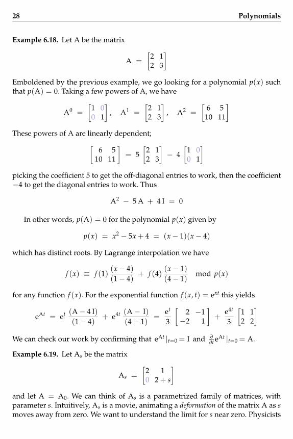
Example 6.18. Let A be the matrix
A =[
2 12 3
]Emboldened by the previous example, we go looking for a polynomial p(x) suchthat p(A) = 0. Taking a few powers of A, we have
A0 =[
1 00 1
], A1 =
[2 12 3
], A2 =
[6 5
10 11
]These powers of A are linearly dependent;[
6 510 11
]= 5
[2 12 3
]− 4
[1 00 1
]picking the coefficient 5 to get the off-diagonal entries to work, then the coefficient−4 to get the diagonal entries to work. Thus
A2 − 5 A + 4 I = 0
In other words, p(A) = 0 for the polynomial p(x) given by
p(x) = x2 − 5x + 4 = (x− 1)(x− 4)
which has distinct roots. By Lagrange interpolation we have
f (x) ≡ f (1)(x− 4)(1− 4)
+ f (4)(x− 1)(4− 1)
mod p(x)
for any function f (x). For the exponential function f (x, t) = ext this yields
eAt = et (A− 4 I)(1− 4)
+ e4t (A− I)(4− 1)
=et
3
[2 −1−2 1
]+
e4t
3
[1 12 2
]We can check our work by confirming that eAt |t=0 = I and ∂
∂t eAt |t=0 = A.
Example 6.19. Let As be the matrix
As =[
2 10 2 + s
]and let A = A0. We can think of As is a parametrized family of matrices, withparameter s. Intuitively, As is a movie, animating a deformation of the matrix A as smoves away from zero. We want to understand the limit for s near zero. Physicists
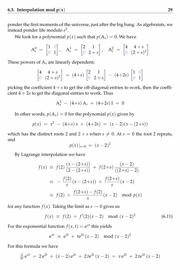
6.3. Interpolation mod p(x) 29
ponder the first moments of the universe, just after the big bang. As algebraists, weinstead ponder life modulo s2.
We look for a polynomial p(x) such that p(As) = 0. We have
A0s =
[1 00 1
], A1
s =[
2 10 2 + s
], A2
s =[
4 4 + s0 (2 + s)2
]These powers of As are linearly dependent;[
4 4 + s0 (2 + s)2
]= (4+s)
[2 10 2 + s
]− (4+2s)
[1 00 1
]picking the coefficient 4 + s to get the off-diagonal entries to work, then the coeffi-cient 4 + 2s to get the diagonal entries to work. Thus
A2s − (4+s) As + (4+2s) I = 0
In other words, p(As) = 0 for the polynomial p(x) given by
p(x) = x2 − (4+s) x + (4+2s) = (x− 2)(x− (2+s))
which has the distinct roots 2 and 2 + s when s 6= 0. At s = 0 the root 2 repeats,and
p(x) |s=0 = (x− 2)2
By Lagrange interpolation we have
f (x) ≡ f (2)(x− (2+s))(2− (2+s))
+ f (2+s)(x− 2)
((2+s)− 2)
≡ − f (2)s
(x− (2+s)) +f (2+s)
s(x− 2)
≡ f (2) +f (2+s)− f (2)
s(x− 2) mod p(x)
for any function f (x). Taking the limit as s→ 0 gives us
f (x) ≡ f (2) + f ′(2)(x− 2) mod (x− 2)2 (6.11)
For the exponential function f (x, t) = ext this yields
ext ≡ e2t + te2t (x− 2) mod (x− 2)2
For this formula we have
∂
∂t ext = 2 e2t + (x− 2) e2t + 2 te2t (x− 2) = x e2t + 2 te2t (x− 2)
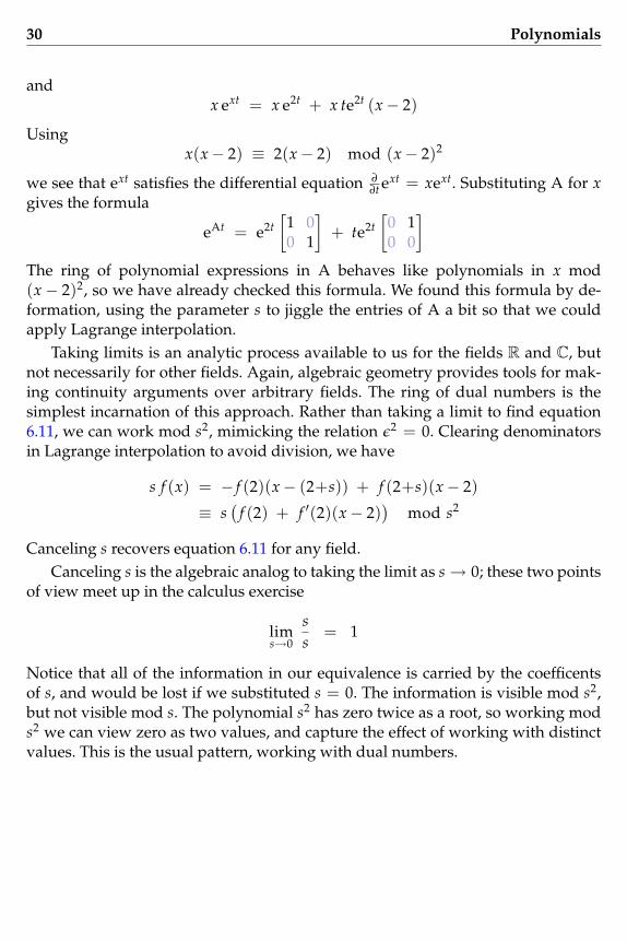
30 Polynomials
andx ext = x e2t + x te2t (x− 2)
Usingx(x− 2) ≡ 2(x− 2) mod (x− 2)2
we see that ext satisfies the differential equation ∂
∂t ext = xext. Substituting A for xgives the formula
eAt = e2t[
1 00 1
]+ te2t
[0 10 0
]The ring of polynomial expressions in A behaves like polynomials in x mod(x− 2)2, so we have already checked this formula. We found this formula by de-formation, using the parameter s to jiggle the entries of A a bit so that we couldapply Lagrange interpolation.
Taking limits is an analytic process available to us for the fields R and C, butnot necessarily for other fields. Again, algebraic geometry provides tools for mak-ing continuity arguments over arbitrary fields. The ring of dual numbers is thesimplest incarnation of this approach. Rather than taking a limit to find equation6.11, we can work mod s2, mimicking the relation ε2 = 0. Clearing denominatorsin Lagrange interpolation to avoid division, we have
s f (x) = − f (2)(x− (2+s)) + f (2+s)(x− 2)
≡ s(
f (2) + f ′(2)(x− 2))
mod s2
Canceling s recovers equation 6.11 for any field.Canceling s is the algebraic analog to taking the limit as s→ 0; these two points
of view meet up in the calculus exercise
lims→0
ss
= 1
Notice that all of the information in our equivalence is carried by the coefficentsof s, and would be lost if we substituted s = 0. The information is visible mod s2,but not visible mod s. The polynomial s2 has zero twice as a root, so working mods2 we can view zero as two values, and capture the effect of working with distinctvalues. This is the usual pattern, working with dual numbers.
Chapter 7
Functions of matrices
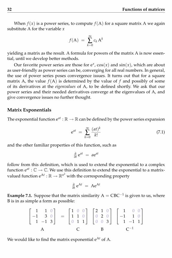
In this chapter, A will always denote a square n× n matrix representing the linearmap L : V → V, where V is an n-dimensional vector space over a field F. Forexample, one can take F to either be the field of real numbers R, in which caseV = Rn, or the field of complex numbers C, in which case V = Cn. In order forpolynomials to have full sets of roots, it will sometimes be necessary to move fromR to C.
We consider the problem of computing functions f (A) of the matrix A, such asthe matrix exponential eAt used to solve systems of linear differential equations.This problem is closely linked to the study of the eigenvalues and eigenvectors of A.
7.1 Polynomials and power series
The functions that we typically want to apply to matrices will either be polynomi-als of the form
f (x) = cd xd + cd−1 xd−1 + . . . + c1 x + c0
or power series of the form
f (x) =∞∑k=0
ck xk
with coefficients in our field F.When f (x) is a polynomial, to compute f (A) for a square matrix A we substi-
tute A for the variable x
f (A) = cd Ad + cd−1 Ad−1 + . . . + c1 A + c0
yielding a matrix as the result. A formula for powers of the matrix A is helpful butnot essential.
32 Functions of matrices
When f (x) is a power series, to compute f (A) for a square matrix A we againsubstitute A for the variable x
f (A) =∞∑k=0
ck Ak
yielding a matrix as the result. A formula for powers of the matrix A is now essen-tial, until we develop better methods.
Our favorite power series are those for ex, cos(x) and sin(x), which are aboutas user-friendly as power series can be, converging for all real numbers. In general,the use of power series poses convergence issues. It turns out that for a squarematrix A, the value f (A) is determined by the value of f and possibly of someof its derivatives at the eigenvalues of A, to be defined shortly. We ask that ourpower series and their needed derivatives converge at the eigenvalues of A, andgive convergence issues no further thought.
Matrix Exponentials
The exponential function eat : R→ R can be defined by the power series expansion
eat =∞∑k=0
(at)k
k!(7.1)
and the other familiar properties of this function, such as
∂
∂t eat = aeat
follow from this definition, which is used to extend the exponential to a complexfunction eat : C → C. We use this definition to extend the exponential to a matrix-valued function eAt : R→ Rn2
with the corresponding property
∂
∂t eAt = AeAt
Example 7.1. Suppose that the matrix similarity A = CBC−1 is given to us, whereB is in as simple a form as possible: 1 1 0
−1 3 01 −1 3
=
1 0 01 1 00 1 1
2 1 00 2 00 0 3
1 0 0−1 1 0
1 −1 1
A C B C−1
We would like to find the matrix exponential eAt of A.
7.1. Polynomials and power series 33
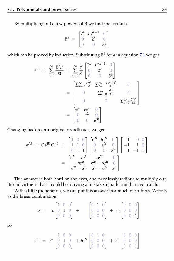
By multiplying out a few powers of B we find the formula
Bk =
2k k 2k−1 00 2k 00 0 3k
which can be proved by induction. Substituting Bk for a in equation 7.1 we get
eBt =∞∑k=0
Bktk
k!=
∞∑k=0
tk
k!
2k k 2k−1 00 2k 00 0 3k
=
∑
∞k=0
2ktk
k! ∑∞k=0
k 2k−1tk
k! 0
0 ∑∞k=0
2ktk
k! 0
0 0 ∑∞k=0
3ktk
k!
=
e2t te2t 00 e2t 00 0 e3t
Changing back to our original coordinates, we get
eAt = C eBt C−1 =
1 0 01 1 00 1 1
e2t te2t 00 e2t 00 0 e3t
1 0 0−1 1 0
1 −1 1
=
e2t − te2t te2t 0−te2t e2t + te2t 0
e3t − e2t e2t − e3t e3t
This answer is both hard on the eyes, and needlessly tedious to multiply out.
Its one virtue is that it could be burying a mistake a grader might never catch.With a little preparation, we can put this answer in a much nicer form. Write B
as the linear combination
B = 2
1 0 00 1 00 0 0
+
0 1 00 0 00 0 0
+ 3
0 0 00 0 00 0 1
so
eBt = e2t
1 0 00 1 00 0 0
+ te2t
0 1 00 0 00 0 0
+ e3t
0 0 00 0 00 0 1
34 Functions of matrices
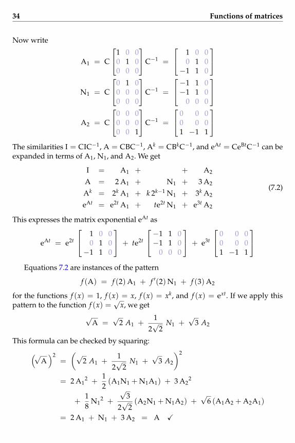
Now write
A1 = C
1 0 00 1 00 0 0
C−1 =
1 0 00 1 0−1 1 0
N1 = C
0 1 00 0 00 0 0
C−1 =
−1 1 0−1 1 0
0 0 0
A2 = C
0 0 00 0 00 0 1
C−1 =
0 0 00 0 01 −1 1
The similarities I = CIC−1, A = CBC−1, Ak = CBkC−1, and eAt = CeBtC−1 can beexpanded in terms of A1, N1, and A2. We get
I = A1 + + A2
A = 2 A1 + N1 + 3 A2
Ak = 2k A1 + k 2k−1 N1 + 3k A2
eAt = e2t A1 + te2t N1 + e3t A2
(7.2)
This expresses the matrix exponential eAt as
eAt = e2t
1 0 00 1 0−1 1 0
+ te2t
−1 1 0−1 1 0
0 0 0
+ e3t
0 0 00 0 01 −1 1
Equations 7.2 are instances of the pattern
f (A) = f (2) A1 + f ′(2) N1 + f (3) A2
for the functions f (x) = 1, f (x) = x, f (x) = xk, and f (x) = ext. If we apply thispattern to the function f (x) =
√x, we get
√A =
√2 A1 +
12√
2N1 +
√3 A2
This formula can be checked by squaring:(√A
)2=
(√2 A1 +
12√
2N1 +
√3 A2
)2
= 2 A12 +
12
(A1N1 + N1A1) + 3 A22
+18
N12 +
√3
2√
2(A2N1 + N1A2) +
√6 (A1A2 + A2A1)
= 2 A1 + N1 + 3 A2 = A X

7.1. Polynomials and power series 35
We have noticed and used the relations
A12 = A1 A2
2 = A2 N12 = 0
A1N1 = N1A1 = N1 A2N1 = N1A2 = 0 A1A2 = A2A1 = 0
This example exhibits behavior typical of the general case of an n× n matrix A.
It would appear in this example that the values 2 and 3 and the matrices A1,N1, and A2 play a fundamental role in the theory of functions of the matrix A. Wehave found these values and matrices by ad hoc means, and that was only afterthe similarity A = CBC−1 was handed to us on a silver platter. This similarity isnontrivial to work out from scratch.
We would like to understand these values and matrices better, and work outfaster ways to compute them. That is the goal of this chapter.
Eigenvalues
Eigenvalues are key to finding matrix similarities such as the similarity A = CBC−1
used in example 7.1.
Definition 7.2. Let A be a square matrix. If
Av = λ v
for some scalar λ and nonzero vector v, then we say that λ is an eigenvalue of A,with eigenvector v.
The matrix A acts on v like multiplication by λ. We can think of v as a “stretchdirection” for A, with stretching factor λ. Eigen is a German word, roughly sug-gesting that these values belong to the matrix A.
In the simplest case, we can find n distinct eigenvalues λ1, . . . , λn for the matrixA, and we can find n matrices A1, . . . , An such that
I = A1 + . . . + AnA = λ1 A1 + . . . + λn An
and we are able to compute the function f of A as
f (A) = f (λ1) A1 + . . . + f (λn) An
This is wonderful. Under function evaluation, the matrix A behaves like the list ofeigenvalues λ1, . . . , λn with the helper matrices A1, . . . , An divvying up the effect.
In exceptional cases which do arise in practice, eigenvalues can repeat, leavingus with m < n distinct eigenvalues λ1, . . . , λm. We can find matrices A1, . . . , Amand N such that
I = A1 + . . . + AmA = λ1 A1 + . . . + λm Am + N
36 Functions of matrices
where N is a nilpotent matrix; see definition 6.4. Here, N` = 0 for some ` boundedby the multiplicity of the eigenvalue of A that repeats the most. One could imaginethat N is present in our first version of these formulas, but we have ` = 1 wheneach eigenvalue of A occurs only once, so N is the zero matrix.
Now, the matrix N and some derivatives of f are involved in the computationof f (A). For example, suppose that in the list λ1, . . . , λn of eigenvalues of A, theeigenvalues λ1 and λ2 are the same. We say that λ1 = λ2 has multiplicity two, andwe work instead with the shorter list of distinct eigenvalues λ1, λ3, . . . , λn. Then
f (A) = f (λ1) A1 + f ′(λ1) N1 + f (λ3) A3 + . . . + f (λn) An (7.3)
where N1 = A1N. In other words, when λ1 occurs twice as an eigenvalue, we needto know both f (λ1) and f ′(λ1) to compute f (A).
This is a frequently occurring pattern in mathematics, and it makes sense if weimagine λ1 and λ2 moving together as real numbers, as we vary the matrix A. Oncethese eigenvalues get close to each other, knowing f (λ1) and f ′(λ1) is pretty muchthe same information as knowing f (λ1) and f (λ2); we can use f ′(λ1) to estimatef (λ2). Once these eigenvalues come together, our original formula can break, butits limit is our new formula, giving the correct answer.
It turns out that the matrix N1 is nilpotent, and
f (λ1) A1 + f ′(λ1) N1
is an instance of the pattern that we saw in equation 6.2. The matrix A1 is a piece ofthe identity matrix I, and N1 is the corresponding piece of the nilpotent matrix N.
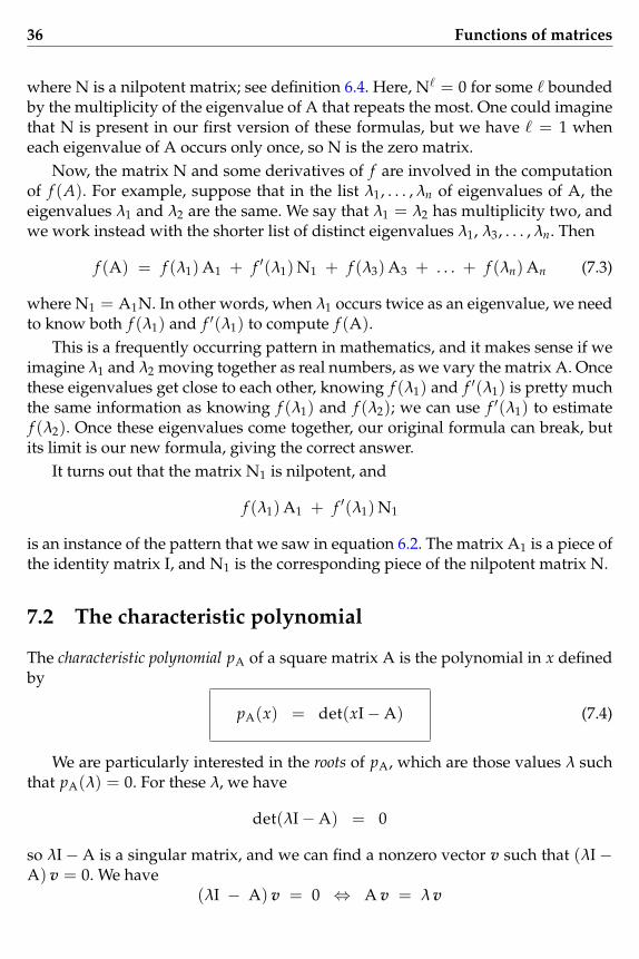
7.2 The characteristic polynomial
The characteristic polynomial pA of a square matrix A is the polynomial in x definedby
pA(x) = det(xI−A) (7.4)
We are particularly interested in the roots of pA, which are those values λ suchthat pA(λ) = 0. For these λ, we have
det(λI−A) = 0
so λI−A is a singular matrix, and we can find a nonzero vector v such that (λI−A) v = 0. We have
(λI − A) v = 0 ⇔ A v = λ v

7.2. The characteristic polynomial 37
In other words, if λ is a root of the polynomial pA, then λ is an eigenvalue of A, witheigenvector v. If we can find a basis of eigenvectors for A, then A can be expressedas a diagonal matrix in terms of this basis.
In general, the characteristic polynomial pA can have repeated roots, and wemay not be able to find a basis of eigenvectors for A. Nevertheless the matrix equa-tion
pA(A) = 0
always holds. This identity is known as the Cayley-Hamilton theorem.Many problems involving the matrix A can be solved either by diagonalizing
A if possible, or by applying the identity pA(A) = 0. Either way, understandingpA is essential to working with the matrix A.
In this section, we develop formulas for computing the characteristic polyno-mial pA.
2× 2 matrices
For the matrix
A =[
a cb d
]we have
pA(x) =∣∣∣∣x− a −c−b x− d
∣∣∣∣ = x2 − (a + d) x + (ad− bc)
This yields the formula
pA(x) = x2 − trace(A) x + det(A) (7.5)
where trace(A) is the sum of the diagonal entries of A.One systematic way to carry out this computation is to write[
x− a−b
]= x
[10
]−
[ab
][
x− c−d
]= x
[01
]−
[cd
]

38 Functions of matrices
and to expand pA(x) by linearity in each column of the determinant:
pA(x) =∣∣∣∣x− a −c−b x− d
∣∣∣∣= x
∣∣∣∣1 −c0 x− d
∣∣∣∣ − ∣∣∣∣a −cb x− d
∣∣∣∣= x
(x
∣∣∣∣1 00 1
∣∣∣∣ − ∣∣∣∣1 c0 d
∣∣∣∣) − (x
∣∣∣∣a 0b 1
∣∣∣∣ − ∣∣∣∣a cb d
∣∣∣∣)=
∣∣∣∣1 00 1
∣∣∣∣ x2 −(∣∣∣∣a 0
b 1
∣∣∣∣ +∣∣∣∣1 c0 d
∣∣∣∣) x +∣∣∣∣a cb d
∣∣∣∣= x2 − (a + d) x +
∣∣∣∣a cb d
∣∣∣∣3× 3 matrices
For the matrix
A =
a d gb e hc f i
we have
pA(x) =
∣∣∣∣∣∣x− a −d −g−b x− e −h−c − f x− i
∣∣∣∣∣∣= x3 − (a + e + i) x2
+ ((ae− bd) + (ai− cg) + (ei− f h)) x− (aei + b f g + cdh− a f h− bdi− ceg)
This yields the formula
pA(x) = x3 − trace(A) x2 + trace(∧2A) x − det(A) (7.6)
where
trace(∧2A) =∣∣∣∣a db e
∣∣∣∣ +∣∣∣∣a gc i
∣∣∣∣ +∣∣∣∣e hf i
∣∣∣∣is the sum of the diagonal 2× 2 minors of A.
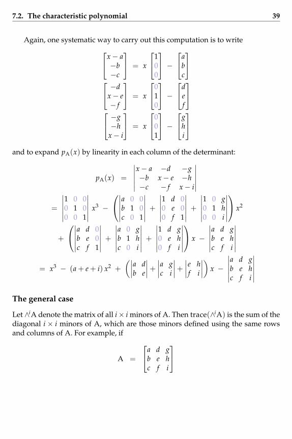
7.2. The characteristic polynomial 39
Again, one systematic way to carry out this computation is to writex− a−b−c
= x
100
−a
bc
−d
x− e− f
= x
010
−d
ef
−g−h
x− i
= x
001
−g
hi
and to expand pA(x) by linearity in each column of the determinant:
pA(x) =
∣∣∣∣∣∣x− a −d −g−b x− e −h−c − f x− i
∣∣∣∣∣∣=
∣∣∣∣∣∣1 0 00 1 00 0 1
∣∣∣∣∣∣ x3 −
∣∣∣∣∣∣a 0 0b 1 0c 0 1
∣∣∣∣∣∣ +
∣∣∣∣∣∣1 d 00 e 00 f 1
∣∣∣∣∣∣ +
∣∣∣∣∣∣1 0 g0 1 h0 0 i
∣∣∣∣∣∣ x2
+
∣∣∣∣∣∣a d 0b e 0c f 1
∣∣∣∣∣∣ +
∣∣∣∣∣∣a 0 gb 1 hc 0 i
∣∣∣∣∣∣ +
∣∣∣∣∣∣1 d g0 e h0 f i
∣∣∣∣∣∣ x −
∣∣∣∣∣∣a d gb e hc f i
∣∣∣∣∣∣= x3 − (a + e + i) x2 +
(∣∣∣∣a db e
∣∣∣∣ +∣∣∣∣a gc i
∣∣∣∣ +∣∣∣∣e hf i
∣∣∣∣) x −
∣∣∣∣∣∣a d gb e hc f i
∣∣∣∣∣∣The general case
Let ∧iA denote the matrix of all i× i minors of A. Then trace(∧iA) is the sum of thediagonal i × i minors of A, which are those minors defined using the same rowsand columns of A. For example, if
A =
a d gb e hc f i
40 Functions of matrices
then
∧2A =
∣∣∣∣a db e
∣∣∣∣ ∣∣∣∣a gb h
∣∣∣∣ ∣∣∣∣d ge h
∣∣∣∣∣∣∣∣a dc f
∣∣∣∣ ∣∣∣∣a gc i
∣∣∣∣ ∣∣∣∣d gf i
∣∣∣∣∣∣∣∣b ec f
∣∣∣∣ ∣∣∣∣b hc i
∣∣∣∣ ∣∣∣∣e hf i
∣∣∣∣
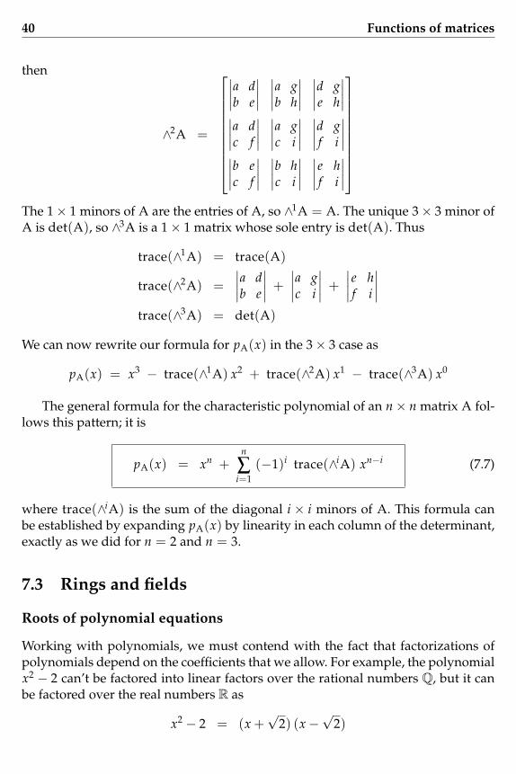
The 1× 1 minors of A are the entries of A, so ∧1A = A. The unique 3× 3 minor ofA is det(A), so ∧3A is a 1× 1 matrix whose sole entry is det(A). Thus
trace(∧1A) = trace(A)
trace(∧2A) =∣∣∣∣a db e
∣∣∣∣ +∣∣∣∣a gc i
∣∣∣∣ +∣∣∣∣e hf i
∣∣∣∣trace(∧3A) = det(A)
We can now rewrite our formula for pA(x) in the 3× 3 case as
pA(x) = x3 − trace(∧1A) x2 + trace(∧2A) x1 − trace(∧3A) x0
The general formula for the characteristic polynomial of an n× n matrix A fol-lows this pattern; it is
pA(x) = xn +n
∑i=1
(−1)i trace(∧iA) xn−i (7.7)
where trace(∧iA) is the sum of the diagonal i × i minors of A. This formula canbe established by expanding pA(x) by linearity in each column of the determinant,exactly as we did for n = 2 and n = 3.
7.3 Rings and fields
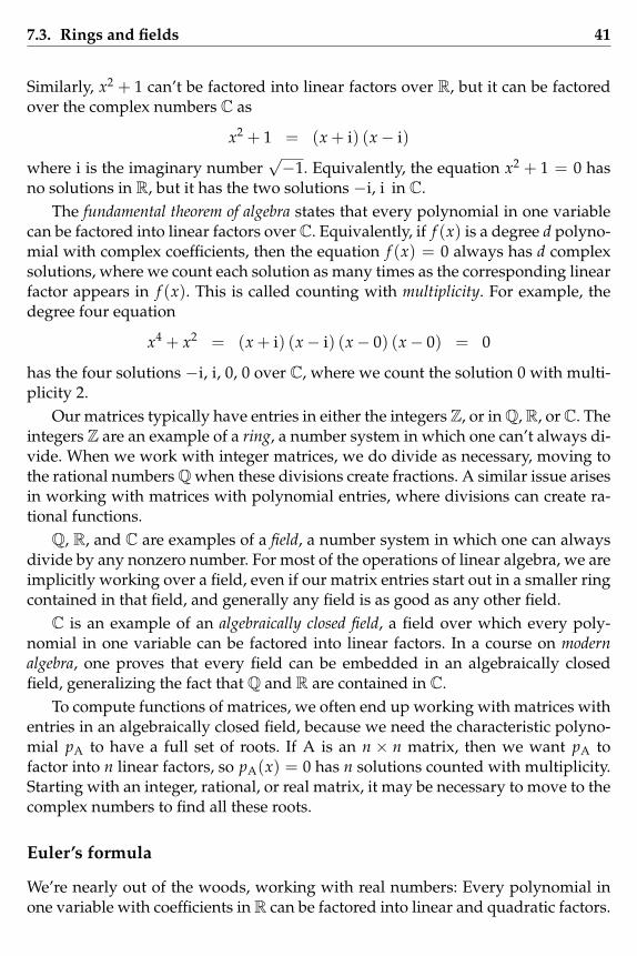
Roots of polynomial equations
Working with polynomials, we must contend with the fact that factorizations ofpolynomials depend on the coefficients that we allow. For example, the polynomialx2 − 2 can’t be factored into linear factors over the rational numbers Q, but it canbe factored over the real numbers R as
x2 − 2 = (x +√
2) (x−√
2)
7.3. Rings and fields 41
Similarly, x2 + 1 can’t be factored into linear factors over R, but it can be factoredover the complex numbers C as
x2 + 1 = (x + i) (x− i)
where i is the imaginary number√−1. Equivalently, the equation x2 + 1 = 0 has
no solutions in R, but it has the two solutions −i, i in C.The fundamental theorem of algebra states that every polynomial in one variable
can be factored into linear factors over C. Equivalently, if f (x) is a degree d polyno-mial with complex coefficients, then the equation f (x) = 0 always has d complexsolutions, where we count each solution as many times as the corresponding linearfactor appears in f (x). This is called counting with multiplicity. For example, thedegree four equation
x4 + x2 = (x + i) (x− i) (x− 0) (x− 0) = 0
has the four solutions −i, i, 0, 0 over C, where we count the solution 0 with multi-plicity 2.
Our matrices typically have entries in either the integers Z, or in Q, R, or C. Theintegers Z are an example of a ring, a number system in which one can’t always di-vide. When we work with integer matrices, we do divide as necessary, moving tothe rational numbers Q when these divisions create fractions. A similar issue arisesin working with matrices with polynomial entries, where divisions can create ra-tional functions.
Q, R, and C are examples of a field, a number system in which one can alwaysdivide by any nonzero number. For most of the operations of linear algebra, we areimplicitly working over a field, even if our matrix entries start out in a smaller ringcontained in that field, and generally any field is as good as any other field.
C is an example of an algebraically closed field, a field over which every poly-nomial in one variable can be factored into linear factors. In a course on modernalgebra, one proves that every field can be embedded in an algebraically closedfield, generalizing the fact that Q and R are contained in C.
To compute functions of matrices, we often end up working with matrices withentries in an algebraically closed field, because we need the characteristic polyno-mial pA to have a full set of roots. If A is an n × n matrix, then we want pA tofactor into n linear factors, so pA(x) = 0 has n solutions counted with multiplicity.Starting with an integer, rational, or real matrix, it may be necessary to move to thecomplex numbers to find all these roots.
Euler’s formula
We’re nearly out of the woods, working with real numbers: Every polynomial inone variable with coefficients in R can be factored into linear and quadratic factors.

42 Functions of matrices
In calculus one studies exponential and trigonometric functions, correspondingto solutions to certain degree one and two differential equations. Ever wonder whythere isn’t some ornate theory that comes next, studying functions that correspondto solutions to certain degree three differential equations? Because real polynomialsfactor into linear and quadratic factors, we can reduce to the study of exponentialand trigonometric functions.
Over the complex numbers, we have Euler’s formula
eix = cos(x) + i sin(x) (7.8)
which can easily be established by comparing power series expansions. Becausecomplex polynomials factor into linear factors, we can reduce to the study of expo-nential functions alone. Euler’s formula expresses how to reduce questions involv-ing trigonometric functions to ones involving complex exponentials.
For example, what were the addition laws for sine and cosine again? We canform the complex exponential
cos(a + b) + i sin(a + b) = ei(a+b)
= eia eib
= (cos(a) + i sin(a))(cos(b) + i sin(b))= (cos(a) cos(b)− sin(a) sin(b))
+ i (cos(a) sin(b) + cos(b) sin(a))
and by taking real and imaginary parts, we get
cos(a + b) = cos(a) cos(b)− sin(a) sin(b)sin(a + b) = cos(a) sin(b) + cos(b) sin(a)
In general, Euler’s formula is a radical simplification of the trigonometric iden-tities. One can understand Euler’s formula as factoring the Pythagorean trigono-metric identity as a difference of squares:
cos2(x) + sin2(x) = (cos(x) + i sin(x)) (cos(x)− i sin(x))
= eixe−ix = 1
This approach really comes into its own for solving integration problems. Com-puter programs for symbolic integration work over C in order to avoid the intrica-cies of trigonometric integration; a broad swath of disparate integration problemscan be viewed uniformly as rational functions of matrix exponentials. Many peoplealso make this migration to C, with the same motivation.
7.4. Diagonal and triangular forms 43
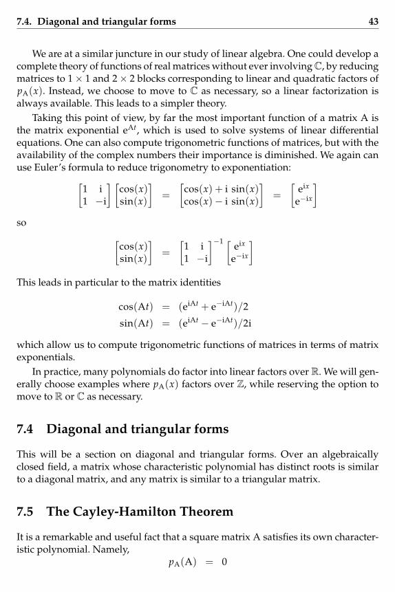
We are at a similar juncture in our study of linear algebra. One could develop acomplete theory of functions of real matrices without ever involving C, by reducingmatrices to 1× 1 and 2× 2 blocks corresponding to linear and quadratic factors ofpA(x). Instead, we choose to move to C as necessary, so a linear factorization isalways available. This leads to a simpler theory.
Taking this point of view, by far the most important function of a matrix A isthe matrix exponential eAt, which is used to solve systems of linear differentialequations. One can also compute trigonometric functions of matrices, but with theavailability of the complex numbers their importance is diminished. We again canuse Euler’s formula to reduce trigonometry to exponentiation:[
1 i1 −i
] [cos(x)sin(x)
]=
[cos(x) + i sin(x)cos(x)− i sin(x)
]=
[eix
e−ix
]so [
cos(x)sin(x)
]=
[1 i1 −i
]−1 [eix
e−ix
]This leads in particular to the matrix identities
cos(At) = (eiAt + e−iAt)/2
sin(At) = (eiAt − e−iAt)/2i
which allow us to compute trigonometric functions of matrices in terms of matrixexponentials.
In practice, many polynomials do factor into linear factors over R. We will gen-erally choose examples where pA(x) factors over Z, while reserving the option tomove to R or C as necessary.
7.4 Diagonal and triangular forms
This will be a section on diagonal and triangular forms. Over an algebraicallyclosed field, a matrix whose characteristic polynomial has distinct roots is similarto a diagonal matrix, and any matrix is similar to a triangular matrix.
7.5 The Cayley-Hamilton Theorem
It is a remarkable and useful fact that a square matrix A satisfies its own character-istic polynomial. Namely,
pA(A) = 0
44 Functions of matrices
In other words, if A is an n× n matrix and
pA(x) = xn + c1 xn−1 + . . . + cn−1 x + cn
then substituting the matrix A for the variable x yields the zero matrix:
An + c1 An−1 + ... + cn−1 A + cn I = 0 (7.9)
We often like to think of matrices as if they are single values, a kind of general-ized number. Bearing in mind the caveats that order of multiplication matters, andthat there are many singular matrices in place of the unique number zero, much canbe learned about matrices by manipulating algebraic expressions involving matrixvalues.
The significance of the Cayley-Hamilton theorem is that all computations in-volving a matrix A can be viewed as taking place modulo pA. Using this result, wewill develop methods that make short work of typical eigenvalue problems suchas computing matrix exponentials.
A formula for the inverse
Equation 7.9 has many applications; one is to express the inverse of an invertiblematrix A as a polynomial in A. We have
cn = pA(0) = det(−A) = (−1)n det(A)
If cn 6= 0, then we can rewrite equation 7.9 as
cnI = − (An−1 + c1 An−2 + ... + cn−1 I) A
so
A−1 = − 1cn
(An−1 + c1 An−2 + ... + cn−1 I) (7.10)
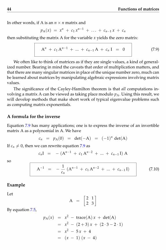
Example
Let
A =[
2 12 3
]By equation 7.5,
pA(x) = x2 − trace(A) x + det(A)
= x2 − (2 + 3) x + (2 · 3− 2 · 1)
= x2 − 5 x + 4= (x − 1) (x − 4)

7.5. The Cayley-Hamilton Theorem 45
so by equation 7.9,
pA(A) = A2 − 5 A + 4 I
=[
2 12 3
]2
− 5[
2 12 3
]+ 4
[1 00 1
]=
[6 5
10 11
]−
[10 510 15
]+
[4 00 4
]=
[0 00 0
]and
pA(A) = (A − I) (A − 4 I)
=([
2 12 3
]−
[1 00 1
]) ([2 12 3
]− 4
[1 00 1
])=
[1 12 2
] [−2 1
2 −1
]=
[0 00 0
]and by equation 7.10,
A−1 = − 14
(A − 5 I)
=14
(−
[2 12 3
]+
[5 00 5
])=
[3 −1−2 2
]/4
One confirms that
A A−1 =[
2 12 3
] [3 −1−2 2
]/4
=[
1 00 1
]= I
2× 2 matrices
One can confirm equation 7.9 by direct computation, for a general 2× 2 matrix. Let
A =[
a cb d
]Then
pA
([a cb d
])=
[a cb d
]2
− (a + d)[
a cb d
]+ (ad− bc)
[1 00 1
]=
[a2 + bc ac + cdab + bd bc + d2
]−
[a2 + ad ac + cdab + bd ad + d2
]+
[ad− bc 0
0 ad− bc
]=
[0 00 0
]
46 Functions of matrices
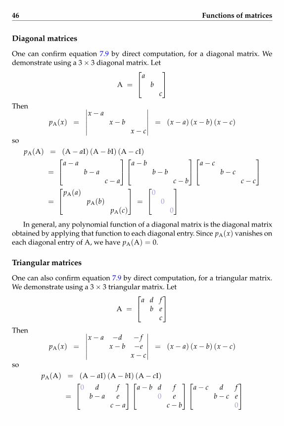
Diagonal matrices
One can confirm equation 7.9 by direct computation, for a diagonal matrix. Wedemonstrate using a 3× 3 diagonal matrix. Let
A =
ab
c
Then
pA(x) =
∣∣∣∣∣∣x− a
x− bx− c
∣∣∣∣∣∣ = (x− a) (x− b) (x− c)
so
pA(A) = (A− aI) (A− bI) (A− cI)
=
a− ab− a
c− a
a− bb− b
c− b
a− cb− c
c− c
=
pA(a)pA(b)
pA(c)
=
00
0
In general, any polynomial function of a diagonal matrix is the diagonal matrix
obtained by applying that function to each diagonal entry. Since pA(x) vanishes oneach diagonal entry of A, we have pA(A) = 0.
Triangular matrices
One can also confirm equation 7.9 by direct computation, for a triangular matrix.We demonstrate using a 3× 3 triangular matrix. Let
A =
a d fb e
c
Then
pA(x) =
∣∣∣∣∣∣x− a −d − f
x− b −ex− c
∣∣∣∣∣∣ = (x− a) (x− b) (x− c)
so
pA(A) = (A− aI) (A− bI) (A− cI)
=
0 d fb− a e
c− a
a− b d f0 e
c− b
a− c d fb− c e
0
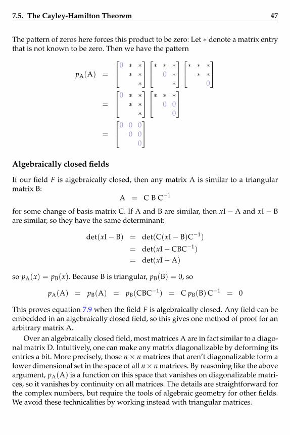
7.5. The Cayley-Hamilton Theorem 47
The pattern of zeros here forces this product to be zero: Let ∗ denote a matrix entrythat is not known to be zero. Then we have the pattern
pA(A) =
0 ∗ ∗∗ ∗∗
∗ ∗ ∗0 ∗∗
∗ ∗ ∗∗ ∗0
=
0 ∗ ∗∗ ∗∗
∗ ∗ ∗0 00
=
0 0 00 0
0
Algebraically closed fields
If our field F is algebraically closed, then any matrix A is similar to a triangularmatrix B:
A = C B C−1
for some change of basis matrix C. If A and B are similar, then xI− A and xI− Bare similar, so they have the same determinant:
det(xI− B) = det(C(xI− B)C−1)
= det(xI− CBC−1)= det(xI−A)
so pA(x) = pB(x). Because B is triangular, pB(B) = 0, so
pA(A) = pB(A) = pB(CBC−1) = C pB(B) C−1 = 0
This proves equation 7.9 when the field F is algebraically closed. Any field can beembedded in an algebraically closed field, so this gives one method of proof for anarbitrary matrix A.
Over an algebraically closed field, most matrices A are in fact similar to a diago-nal matrix D. Intuitively, one can make any matrix diagonalizable by deforming itsentries a bit. More precisely, those n× n matrices that aren’t diagonalizable form alower dimensional set in the space of all n× n matrices. By reasoning like the aboveargument, pA(A) is a function on this space that vanishes on diagonalizable matri-ces, so it vanishes by continuity on all matrices. The details are straightforward forthe complex numbers, but require the tools of algebraic geometry for other fields.We avoid these technicalities by working instead with triangular matrices.
48 Functions of matrices
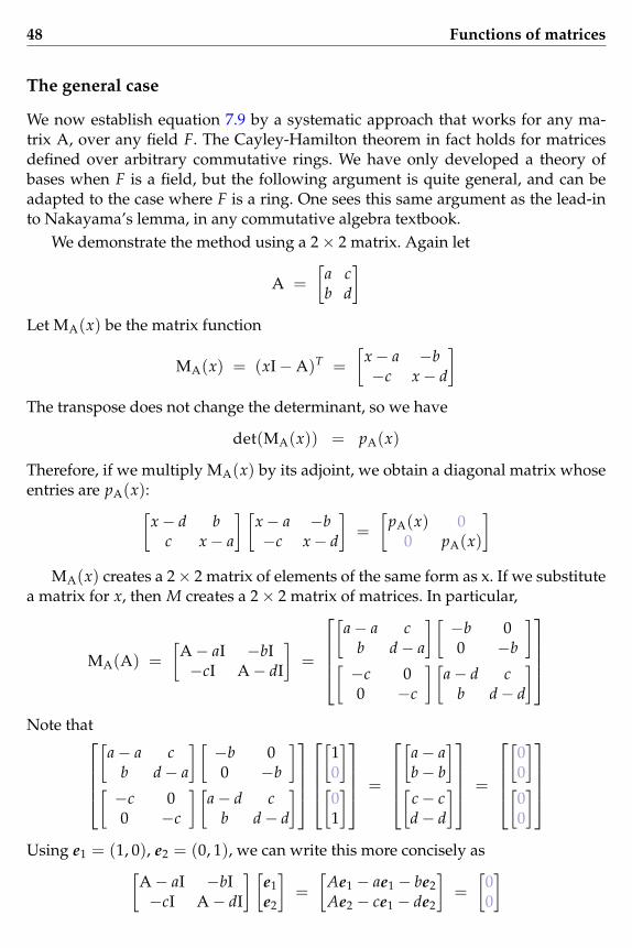
The general case
We now establish equation 7.9 by a systematic approach that works for any ma-trix A, over any field F. The Cayley-Hamilton theorem in fact holds for matricesdefined over arbitrary commutative rings. We have only developed a theory ofbases when F is a field, but the following argument is quite general, and can beadapted to the case where F is a ring. One sees this same argument as the lead-into Nakayama’s lemma, in any commutative algebra textbook.
We demonstrate the method using a 2× 2 matrix. Again let
A =[
a cb d
]Let MA(x) be the matrix function
MA(x) = (xI−A)T =[
x− a −b−c x− d
]The transpose does not change the determinant, so we have
det(MA(x)) = pA(x)
Therefore, if we multiply MA(x) by its adjoint, we obtain a diagonal matrix whoseentries are pA(x):[
x− d bc x− a
] [x− a −b−c x− d
]=
[pA(x) 0
0 pA(x)
]MA(x) creates a 2× 2 matrix of elements of the same form as x. If we substitute
a matrix for x, then M creates a 2× 2 matrix of matrices. In particular,
MA(A) =[
A− aI −bI−cI A− dI
]=
[
a− a cb d− a
][−b 00 −b
][−c 00 −c
][a− d c
b d− d
]
Note that[
a− a cb d− a
][−b 00 −b
][−c 00 −c
][a− d c
b d− d
]
[
10
][
01
] =
[
a− ab− b
][
c− cd− d
] =
[
00
][
00
]
Using e1 = (1, 0), e2 = (0, 1), we can write this more concisely as[A− aI −bI−cI A− dI
] [e1e2
]=
[Ae1 − ae1 − be2Ae2 − ce1 − de2
]=
[00
]
7.6. Repeated roots 49
Now, multiply MA(A) by its adjoint:[A− dI bI
cI A− aI
] [A− aI −bI−cI A− dI
]=
[pA(A) 0
0 pA(A)
]Putting this together, we have[
pA(A) 00 pA(A)
] [e1e2
]=
[pA(A) e1pA(A) e2
]=
[00
]Since pA(A) maps the basis e1, e2 to 0, it must be the zero matrix.
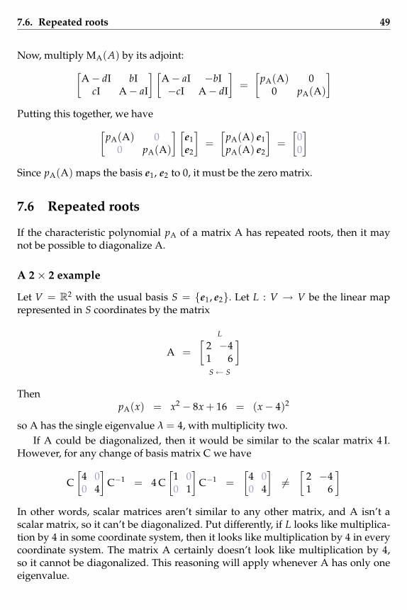
7.6 Repeated roots
If the characteristic polynomial pA of a matrix A has repeated roots, then it maynot be possible to diagonalize A.
A 2× 2 example
Let V = R2 with the usual basis S = {e1, e2}. Let L : V → V be the linear maprepresented in S coordinates by the matrix
L
A =[
2 −41 6
]S← S
ThenpA(x) = x2 − 8x + 16 = (x− 4)2
so A has the single eigenvalue λ = 4, with multiplicity two.If A could be diagonalized, then it would be similar to the scalar matrix 4 I.
However, for any change of basis matrix C we have
C[
4 00 4
]C−1 = 4 C
[1 00 1
]C−1 =
[4 00 4
]6=
[2 −41 6
]In other words, scalar matrices aren’t similar to any other matrix, and A isn’t ascalar matrix, so it can’t be diagonalized. Put differently, if L looks like multiplica-tion by 4 in some coordinate system, then it looks like multiplication by 4 in everycoordinate system. The matrix A certainly doesn’t look like multiplication by 4,so it cannot be diagonalized. This reasoning will apply whenever A has only oneeigenvalue.
50 Functions of matrices
Let
B = A− 4 I =[−2 −4
1 2
]B is indeed singular, as expected because pA(4) = 0. The nullspace of B is theeigenspace of A with eigenvalue λ = 4. For A to have a basis of eigenvectorsv1, v2, this nullspace would have to have dimension two, so B would have to haverank zero. However, only the zero matrix has rank zero. B is not the zero matrix, sowe again see that A cannot be diagonalized.
This means that we cannot find two linearly independent vectors v1, v2 suchthat
v1B−−→ 0, v2
B−−→ 0
However, by the Cayley-Hamilton theorem,
pA(A) = (A− 4 I)2 = B2 = 0
so B2 is the zero matrix, as we would have liked for B itself. We check this. Indeed,
B2 =[−2 −4
1 2
][−2 −4
1 2
]=
[0 00 0
]X
It would be nice if we could simply choose an arbitrary basis for the nullspaceof B2 and be done. However, S is already such a basis, and the appearance of Aisn’t exactly illuminating. We can do better.
The best we can do is to find a basis of vectors v1, v2 forming a chain
v2B−−→ v1
B−−→ 0
In terms of such a basis T = {v1, v2} we have
Av1 = (4 I + B) v1 = 4 v1 + 0Av2 = (4 I + B) v2 = 4 v2 + v1
allowing us to represent the linear map L in T coordinates by the matrix
L
E =[
4 10 4
]T ← T
This matrix E is in Jordan canonical form.
7.6. Repeated roots 51
Any vector v2 that is not in the nullspace of B will yield the desired chain. Forexample, the standard basis vectors e1, e2 can’t both be in the nullspace of B, so wetry both of them:
e1 = (1, 0) B−−→ (−2, 1) B−−→ 0
e2 = (0, 1) B−−→ (−4, 2) B−−→ 0
We prefer the first chain; it leads to a simpler basis, with a change of basis matrixhaving determinant 1. Had we balked at using either of these chains, we couldhave chosen a nice solution to Bv1 = 0, and then solved Bv2 = v1.
We have found the basis T given by
v1 = (−2, 1), v2 = (1, 0)
Let C be the change of basis matrix with columns v1, v2. Then we have the changeof basis
L I L I[2 −41 6
]=
[−2 1
1 0
] [4 10 4
] [0 11 2
]S← S S← T T ← T T ← S
A C E C−1
We can expand E as the linear combination E = 4 I + N of the identity matrixand a nilpotent matrix N [
4 10 4
]= 4
[1 00 1
]+
[0 10 0
]Changing back to S coordinates, we expand
A = C E C−1 = C (4 I + N) C−1 = 4 C I C−1 + C N C−1
This gives us[2 −41 6
]= 4
[−2 1
1 0
] [1 00 1
] [0 11 2
]︸ ︷︷ ︸ +
[−2 1
1 0
] [0 10 0
] [0 11 2
]︸ ︷︷ ︸
= 4[
1 00 1
]+
[−2 −4
1 2
]expressing our original matrix A as the same linear combination of the identitymatrix and the nilpotent matrix B. Seeing that this is where we ended up, it wouldseem that we could have skipped right to this step.
52 Functions of matrices
Indeed, we have
A = C E C−1 ⇒ An = C En C−1
A = λ I + B ⇒ An = λn I + n λn−1 B
using B2 = 0. The first implication expands into the second, and either can be usedto compute functions of A: We have
En =[
4 10 4
]n
=[
4n n 4n−1
0 4n
]= 4n
[1 00 1
]+ n 4n−1
[0 10 0
]so
An = 4n[
1 00 1
]+ n 4n−1
[−2 −4
1 2
]

Chapter 8
Inner products
Lorem ipsum dolor sit amet, consectetur adipisicing elit, sed do eiusmod temporincididunt ut labore et dolore magna aliqua. Ut enim ad minim veniam, quis nos-trud exercitation ullamco laboris nisi ut aliquip ex ea commodo consequat. Duisaute irure dolor in reprehenderit in voluptate velit esse cillum dolore eu fugiatnulla pariatur. Excepteur sint occaecat cupidatat non proident, sunt in culpa quiofficia deserunt mollit anim id est laborum.

Index
algebraic geometry, 19, 23, 30algebraically closed field, 41
big bang, 29
Cayley-Hamilton theorem, 37, 50characteristic polynomial, 36companion matrix, 16
deformation, 28, 30determinant, 7dual numbers, 14, 30
eigenvalue, 23, 31, 32, 35, 37eigenvector, 31, 35, 37Euler’s formula, 42
field, 41fundamental theorem of algebra, 41
integral domain, 18
Jordan canonical form, 50
Lagrange form, 24Lagrange interpolation, 20, 24, 25Linear algebra, vlong division, 18
matrix, vnilpotent, 51scalar, 49
matrix exponential, 32modern algebra, iii, 41multiplicity, 41
nilpotent, 14nilpotent matrix, 36noncommutative, vi
rational canonical form, 16ring, 41roots, 36
repeated, 49
Vandermonde matrix, 20, 21vectors, v