Linear Predictive Coding

Jeremy Bradbury

December 5, 2000

1

0 Outline

I. Proposal

II. Introduction

A. Speech Coding

B. Voice Coders

C. LPC Overview

III. Historical Perspective of Linear Predictive Coding

A. History of Speech & Audio Compression

B. History of Speech Synthesis

C. Analysis/Synthesis Techniques

IV. Human Speech Production

V. LPC Model

VI. LPC Analysis/Encoding

A. Input speech

B. Voice/Unvoiced Determination

C. Pitch Period Estimation

D. Vocal Tract Filter

E. Transmitting the Parameters

VII. LPC Synthesis/Decoding

VIII. LPC Applications

A. Telephone Systems

B. Text-to-Speech Synthesis

C. Voice Mail Systems

D. Multimedia

IX. Conclusion

X. References

2

1 Proposal

Linear predictive coding(LPC) is defined as a digital method for encoding an analog signal

in which a particular value is predicted by a linear function of the past values of the signal. It was first

proposed as a method for encoding human speech by the United States Department of Defence in

federal standard 1015, published in 1984. Human speech is produced in the vocal tract which can be

approximated as a variable diameter tube. The linear predictive coding (LPC) model is based on a

mathematical approximation of the vocal tract represented by this tube of a varying diameter. At a

particular time, t, the speech sample s(t) is represented as a linear sum of the p previous samples. The

most important aspect of LPC is the linear predictive filter which allows the value of the next sample

to be determined by a linear combination of previous samples. Under normal circumstances, speech

is sampled at 8000 samples/second with 8 bits used to represent each sample. This provides a rate of

64000 bits/second. Linear predictive coding reduces this to 2400 bits/second. At this reduced rate

the speech has a distinctive synthetic sound and there is a noticeable loss of quality. However, the

speech is still audible and it can still be easily understood. Since there is information loss in linear

predictive coding, it is a lossy form of compression.

I will describe the necessary background needed to understand how the vocal tract produces

speech. I will also explain how linear predictive coding mathematically approximates the parameters

of the vocal tract to reduce a speech signal to a state that is noticeably synthetic but still

understandable. I will conclude by discussing other speech encoding schemes that have been based

on LPC and by discussing possible disadvantages and applications of the LPC model.

3

2 Introduction

There exist many different types of speech compression that make use of a variety of different

techniques. However, most methods of speech compression exploit the fact that speech production

occurs through slow anatomical movements and that the speech produced has a limited frequency

range. The frequency of human speech production ranges from around 300 Hz to 3400 Hz. Speech

compression is often referred to as speech coding which is defined as a method for reducing the

amount of information needed to represent a speech signal. Most forms of speech coding are usually

based on a lossy algorithm. Lossy algorithms are considered acceptable when encoding speech

because the loss of quality is often undetectable to the human ear.

There are many other characteristics about speech production that can be exploited by speech

coding algorithms. One fact that is often used is that period of silence take up greater than 50% of

conversations. An easy way to save bandwidth and reduce the amount of information needed to

represent the speech signal is to not transmit the silence. Another fact about speech production that

can be taken advantage of is that mechanically there is a high correlation between adjacent samples

of speech. Most forms of speech compression are achieved by modelling the process of speech

production as a linear digital filter. The digital filter and its slow changing parameters are usually

encoded to achieve compression from the speech signal.

Linear Predictive Coding (LPC) is one of the methods of compression that models the process

of speech production. Specifically, LPC models this process as a linear sum of earlier samples using

a digital filter inputting an excitement signal. An alternate explanation is that linear prediction filters

attempt to predict future values of the input signal based on past signals. LPC “...models speech as

an autoregressive process, and sends the parameters of the process as opposed to sending the speech

itself” [4]. It was first proposed as a method for encoding human speech by the United States

Department of Defence in federal standard 1015, published in 1984. Another name for federal

standard 1015 is LPC-10 which is the method of Linear predictive coding that will be described in

this paper.

Speech coding or compression is usually conducted with the use of voice coders or vocoders.

There are two types of voice coders: waveform-following coders and model-base coders. Waveform-

following coders will exactly reproduce the original speech signal if no quantization errors occur.

Model-based coders will never exactly reproduce the original speech signal, regardless of the

4

presence of quantization errors, because they use a parametric model of speech production which

involves encoding and transmitting the parameters not the signal. LPC vocoders are considered

model-based coders which means that LPC coding is lossy even if no quantization errors occur.

All vocoders, including LPC vocoders, have four main attributes: bit rate, delay, complexity,

quality. Any voice coder, regardless of the algorithm it uses, will have to make trade offs between

these different attributes. The first attribute of vocoders, the bit rate, is used to determine the degree

of compression that a vocoder achieves. Uncompressed speech is usually transmitted at 64 kb/s using

8 bits/sample and a rate of 8 kHz for sampling. Any bit rate below 64 kb/s is considered compression.

The linear predictive coder transmits speech at a bit rate of 2.4 kb/s, an excellent rate of compression.

Delay is another important attribute for vocoders that are involved with the transmission of an

encoded speech signal. Vocoders which are involved with the storage of the compressed speech, as

opposed to transmission, are not as concern with delay. The general delay standard for transmitted

speech conversations is that any delay that is greater than 300 ms is considered unacceptable. The

third attribute of voice coders is the complexity of the algorithm used. The complexity affects both

the cost and the power of the vocoder. Linear predictive coding because of its high compression rate

is very complex and involves executing millions of instructions per second. LPC often requires more

than one processor to run in real time. The final attribute of vocoders is quality. Quality is a subjective

attribute and it depends on how the speech sounds to a given listener. One of the most common test

for speech quality is the absolute category rating (ACR) test. This test involves subjects being given

pairs of sentences and asked to rate them as excellent, good, fair, poor, or bad. Linear predictive

coders sacrifice quality in order to achieve a low bit rate and as a result often sound synthetic. An

alternate method of speech compression called adaptive differential pulse code modulation (ADPCM)

only reduces the bit rate by a factor of 2 to 4, between 16 kb/s and 32kb/s , but has a much higher

quality of speech than LPC.

The general algorithm for linear predictive coding involves an analysis or encoding part and

a synthesis or decoding part. In the encoding, LPC takes the speech signal in blocks or frames of

speech and determines the input signal and the coefficients of the filter that will be capable of

reproducing the current block of speech. This information is quantized and transmitted. In the

decoding, LPC rebuilds the filter based on the coefficients received. The filter can be thought of as

a tube which, when given an input signal, attempts to output speech. Additional information about

the original speech signal is used by the decoder to determine the input or excitation signal that is sent

5

Figure 1: Homer Dudley andhis vocoder

to the filter for synthesis.

3 Historical Perspective of Linear Predictive Coding

The history of audio and music compression begin in the 1930s with research into pulse-code

modulation (PCM) and PCM coding. Compression of digital audio was started in the 1960s by

telephone companies who were concerned with the cost of transmission bandwidth. Linear Predictive

Coding’s origins begin in the 1970s with the development of the first LPC algorithms. Adaptive

Differential Pulse Code Modulation (ADPCM), another method of speech coding, was also first

conceived in the 1970s. In 1984, the United States Department of Defence produced federal standard

1015 which outlined the details of LPC. Extensions of LPC such as Code Excited Linear Predictive

(CELP) algorithms and Vector Selectable Excited Linear Predictive (VSELP) algorithms were

developed in the mid 1980s and used commercially for audio music coding in the later part of that

decade. The 1990s have seen improvements in these earlier algorithms and an increase in compression

ratios at given audio quality levels.

The history of speech coding makes no mention of LPC until

the 1970s. However, the history of speech synthesis shows that the

beginnings of Linear Predictive Coding occurred 40 years earlier in

the late 1930s. The first vocoder was described by Homer Dudley in

1939 at Bell Laboratories. A picture of Homer Dudley and his

vocoder can be seen in Figure 1. Dudley developed his vocoder,

called the Parallel Bandpass Vocoder or channel vocoder, to do

speech analysis and resynthesis. LPC is a descendent of this channel

vocoder. The analysis/synthesis scheme used by Dudley is the scheme

of compression that is used in many types of speech compression such

as LPC. The synthesis part of this scheme was first used even earlier

than the 1930s by Kempelen Farkas Lovag (1734-1804). He used it

to make the first machine that could speak. The machine was constructed using a bellow which forced

air through a flexible tube to produce sound.

Analysis/Synthesis schemes are based on the development of a parametric model during the

analysis of the original signal which is later used for the synthesis of the source output. The

transmitter or sender analyses the original signal and acquires parameters for the model which are

6

Figure 2: Path of Human Speech Production

sent to the receiver. The receiver then uses the model and the parameters it receives to synthesize an

approximation of the original signal. Historically, this method of sending the model parameters to the

receiver was the earliest form of lossy speech compression. Other forms of lossy speech compression

that involve sending estimates of the original signal weren’t developed until much later.

4 Human Speech Production

Regardless of the language spoken, all people use relatively the same anatomy to produce

sound. The output produced by each human’s anatomy is limited by the laws of physics.

The process of speech production in humans can be summarized as air being pushed from the

lungs, through the vocal tract, and out through the mouth to generate speech. In this type of

description the lungs can be thought of as the source of the sound and the vocal tract can be thought

of as a filter that produces the various types of sounds that make up speech. The above is a

simplification of how sound is really produced.

In order to understand how the vocal tract turns the air from the lungs into sound it is

important to understand several key definitions. Phonemes are defined as a limited set of individual

7

sounds. There are two categories of phonemes, voiced and unvoiced sounds, that are considered by

the Linear predictive coder when analysing and synthesizing speech signals.

Voiced sounds are usually vowels and often have high average energy levels and very distinct

resonant or formant frequencies. Voiced sounds are generated by air from the lungs being forced over

the vocal cords. As a result the vocal cords vibrate in a somewhat periodically pattern that produces

a series of air pulses called glottal pulses. The rate at which the vocal cords vibrate is what determines

the pitch of the sound produced. These air pulse that are created by the vibrations finally pass along

the rest of the vocal tract where some frequencies resonate. It is generally known that women and

children have higher pitched voices than men as a result of a faster rate of vibration during the

production of voiced sounds. It is therefore important to include the pitch period in the analysis and

synthesis of speech if the final output is expected to accurately represent the original input signal.

Unvoiced sounds are usually consonants and generally have less energy and higher frequencies

then voiced sounds. The production of unvoiced sound involves air being forced through the vocal

tract in a turbulent flow. During this process the vocal cords do not vibrate, instead, they stay open

until the sound is produced. Pitch is an unimportant attribute of unvoiced speech since there is no

vibration of the vocal cords and no glottal pulses.

The categorization of sounds as voiced or unvoiced is an important consideration in the

analysis and synthesis process. In fact, the vibration of the vocal cords, or lack of vibration, is one of

the key components in the production of different types of sound. Another component that influences

speech production is the shape of the vocal tract itself. Different shapes will produce different sounds

or resonant frequencies. The vocal tract consists of the throat, the tongue, the nose, and the mouth.

It is defined as the speech producing path through the vocal organs. This path shapes the frequencies

of the vibrating air travelling through it. As a person speaks, the vocal tract is constantly changing

shape at a very slow rate to produce different sounds which flow together to create words.

A final component that affects the production of sound in humans is the amount of air that

originates in the lungs. The air flowing from the lungs can be though of as the source for the vocal

tract which act as a filter by taking in the source and producing speech. The higher the volume of air

that goes through the vocal tract, the louder the sound.

The idea of the air from the lungs as a source and the vocal tract as a filter is called the

source-filter model for sound production. The source-filter model is the model that is used in linear

predictive coding. It is based on the idea of separating the source from the filter in the production of

8

sound. This model is used in both the encoding and the decoding of LPC and is derived from a

mathematical approximation of the vocal tract represented as a varying diameter tube. The excitation

of the air travelling through the vocal tract is the source. This air can be periodic, when producing

voiced sounds through vibrating vocal cords, or it can be turbulent and random when producing

unvoiced sounds. The encoding process of LPC involves determining a set of accurate parameters

for modelling the vocal tract during the production of a given speech signal. Decoding involves using

the parameters acquired in the encoding and analysis to build a synthesized version of the original

speech signal. LPC never transmits any estimates of speech to the receiver, it only sends the model

to produce the speech and some indications about what type of sound is being produced. In A

Practical Handbook for Speech Coders, Randy Goldberg and Lance Riek define the process of

modelling speech production as a general concept of modelling any type of sound wave in any

medium. “Sound waves are pressure variations that propagate through air (or any other medium) by

the vibrations of the air particles. Modelling these waves and their propagation through the vocal tract

provides a framework for characterizing how the vocal tract shapes the frequency content of the

excitation signal” [7].

5 LPC Model

The particular source-filter model used in LPC is known as the Linear predictive coding

model. It has two key components: analysis or encoding and synthesis or decoding. The analysis part

of LPC involves examining the speech signal and breaking it down into segments or blocks. Each

segment is than examined further to find the answers to several key questions:

• Is the segment voiced or unvoiced?

• What is the pitch of the segment?

• What parameters are needed to build a filter that models the vocal tract

for the current segment?

LPC analysis is usually conducted by a sender who answers these questions and usually transmits

these answers onto a receiver. The receiver performs LPC synthesis by using the answers received

to build a filter that when provided the correct input source will be able to accurately reproduce the

9

Figure 3: Human vs. Voice Coder Speech Production

original speech signal. Essentially, LPC synthesis tries to imitate human speech production. Figure

3 demonstrates what parts of the receiver correspond to what parts in the human anatomy. This

diagram is for a general voice or speech coder and is not specific to linear predictive coding. All voice

coders tend to model two things: excitation and articulation. Excitation is the type of sound that is

passed into the filter or vocal tract and articulation is the transformation of the excitation signal into

speech.

6 LPC Analysis/Encoding

Input speech

According to government standard 1014, also known as LPC-10, the input signal is sampled

at a rate of 8000 samples per second. This input signal is then broken up into segments or blocks

which are each analysed and transmitted to the receiver. The 8000 samples in each second of speech

10

Figure 4: Voiced sound – Letter “e” in the word “test”

Figure 5: Unvoiced sound – Letter “s” in the word “test”

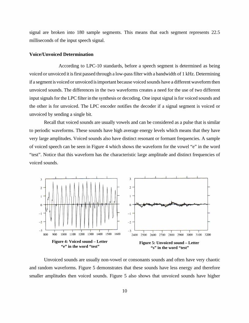
signal are broken into 180 sample segments. This means that each segment represents 22.5

milliseconds of the input speech signal.

Voice/Unvoiced Determination

According to LPC-10 standards, before a speech segment is determined as being

voiced or unvoiced it is first passed through a low-pass filter with a bandwidth of 1 kHz. Determining

if a segment is voiced or unvoiced is important because voiced sounds have a different waveform then

unvoiced sounds. The differences in the two waveforms creates a need for the use of two different

input signals for the LPC filter in the synthesis or decoding. One input signal is for voiced sounds and

the other is for unvoiced. The LPC encoder notifies the decoder if a signal segment is voiced or

unvoiced by sending a single bit.

Recall that voiced sounds are usually vowels and can be considered as a pulse that is similar

to periodic waveforms. These sounds have high average energy levels which means that they have

very large amplitudes. Voiced sounds also have distinct resonant or formant frequencies. A sample

of voiced speech can be seen in Figure 4 which shows the waveform for the vowel “e” in the word

“test”. Notice that this waveform has the characteristic large amplitude and distinct frequencies of

voiced sounds.

Unvoiced sounds are usually non-vowel or consonants sounds and often have very chaotic

and random waveforms. Figure 5 demonstrates that these sounds have less energy and therefore

smaller amplitudes then voiced sounds. Figure 5 also shows that unvoiced sounds have higher

11

frequencies then voiced sounds.

There are two steps in the process of determining if a speech segment is voiced or unvoiced.

The first step is to look at the amplitude of the signal, also known as the energy in the segment. If

the amplitude levels are large then the segment is classified as voiced and if they are small then the

segment is considered unvoiced. This determination requires a preconceived notion about the range

of amplitude values and energy levels associated with the two types of sound.

In order to help determine a classification for sounds that can not be clearly classified based

on an analysis of the amplitude, a second step is used to make the final distinction between voiced

and unvoiced sounds. This step takes advantage of the fact that voiced speech segments have large

amplitudes, unvoiced speech segments have high frequencies, and that the average values of both

types of speech samples is close to zero. These three facts lead to the conclusion that the unvoiced

speech waveform must cross the x-axis more often then the waveform of voiced speech. This can

clearly be seen to be true in the case of Figure 4 and Figure 5. Thus, the determination of voiced and

unvoiced speech signals is finalized by counting the number of times a waveform crosses the x-axis

and then comparing that value to the normally range of values for most unvoiced and voiced sounds.

An additional factor that influences this classification is the surrounding segments. The

classification of these neighbouring segments is taken into consideration because it is undesirable to

have an unvoiced frame in the middle of a group of voiced frames or vice versa.

It is important to realize that sound isn’t always produced according to the LPC model. One

example of this occurs when segments of voiced speech with a lot of background noise are sometimes

interpreted as unvoiced segments. Another case of misinterpretation by the LPC model is with a

group of sounds known as nasal sounds. During the production of these sounds the nose cavity

destroys the concept of a linear tube since the tube now has a branch. This problem is often ignored

in LPC but taken care of in other speech models which have the flexibility of higher bit rates.

Not only is it possible to have sounds that are not produced according to the model, it is also

possible to have sounds that are produced according to the model but that can not be accurately

classified as voiced or unvoiced. These sounds are a combination of the chaotic waveforms of

unvoiced sounds and the periodic waveforms of voiced sounds. The LPC Model can not accurately

reproduce these sounds Examples of such sounds are “this zoo” and “azure”.

Another type of speech encoding called code excited linear prediction coding (CELP) handles

the problem of sounds that are combinations of voiced and unvoiced by using a standard codebook

12

which contains typical problematic signals. In the LPC model, only two different default signals are

used to excite the filter for unvoiced and voiced signals in the decoder. In the CELP model, the

encoder or synthesizer would compare a given waveform to the codebook and find the closest

matching entry. This entry would be sent to the decoder which takes the entry code that is received

and gets the corresponding entry from its codebook and uses this entry to excite the formant filter

instead of one of the default signals used by LPC. CELP has a minimum of 4800 bits/second and can

therefore afford to use a codebook. In LPC, which has half of the bit rate of CELP, the occasionally

transmission of segments with problematic waveforms that will not be accurately reproduced by the

decoder is considered an acceptable error.

Pitch Period Estimation

Determining if a segment is a voiced or unvoiced sound is not all of the information that is

needed by the LPC decoder to accurately reproduce a speech signal. In order to produce an input

signal for the LPC filter the decoder also needs another attribute of the current speech segment

known as the pitch period. The period for any wave, including speech signals, can be defined as the

time required for one wave cycle to completely pass a fixed position. For speech signals, the pitch

period can be thought of as the period of the vocal cord vibration that occurs during the production

of voiced speech. Therefore, the pitch period is only needed for the decoding of voiced segments and

is not required for unvoiced segments since they are produced by turbulent air flow not vocal cord

vibrations.

It is very computationally intensive to determine the pitch period for a given segment of

speech. There are several different types of algorithms that could be used. One type of algorithm

takes advantage of the fact that the autocorrelation of a period function, Rxx(k), will have a maximum

when k is equivalent to the pitch period. These algorithms usually detect a maximum value by

checking the autocorrelation value against a threshold value. One problem with algorithms that use

autocorrelation is that the validity of their results is susceptible to interference as a result of other

resonances in the vocal tract. When interference occurs the algorithm can not guarantee accurate

results. Another problem with autocorrelation algorithms occurs because voiced speech is not entirely

periodic. This means that the maximum will be lower than it should be for a true periodic signal.

LPC-10 does not use an algorithm with autocorrelation, instead it uses an algorithm called

average magnitude difference function (AMDF) which is defined as

13

Figure 6: AMDF function for voiced sound – Letter “e” in the word “test”

Figure 7: AMDF function for unvoicedsound – Letter “s” in the word “test”

Since the pitch period, P, for humans is limited, the AMDF is evaluated for a limited range of the

possible pitch period values. Therefore, in LPC-10 there is an assumption that the pitch period is

between 2.5 and 19.5 milliseconds. If the signal is sampled at a rate of 8000 samples/second then 20

# P # 160.

For voiced segments we can consider the set of speech samples for the current segment, {yn},

as a periodic sequence with period Po. This means that samples that are Po apart should have similar

values and that the AMDF function will have a minimum at Po, that is when P is equal to the pitch

period. An example of the AMDF function applied to the letter “e” from the word “test” can be seen

in Figure 6. If this waveform is compared with the waveform for “e” before the AMDF function is

applied, in Figure 4, it can be seen that this function smooths out the waveform.

An advantage of the AMDF function is that it can be used to determine if a sample is voiced

or unvoiced. When the AMDF function is applied to an unvoiced signal, the difference between the

minimum and the average values is very small compared to voiced signals. This difference can be used

to make the voiced and unvoiced determination. For unvoiced segments the AMDF function we also

have a minimum when P equals the pitch period however, any additional minimums that are obtained

will be very close to the average value. This means that these minimums will not be very deep. An

example of the AMDF function applied to the letter “s” from the word “test” can be seen in Figure

14

7.

Vocal Tract Filter

The filter that is used by the decoder to recreate the original input signal is created based on

a set of coefficients. These coefficients are extracted from the original signal during encoding and are

transmitted to the receiver for use in decoding. Each speech segment has different filter coefficients

or parameters that it uses to recreate the original sound. Not only are the parameters themselves

different from segment to segment, but the number of parameters differ from voiced to unvoiced

segment. Voiced segments use 10 parameters to build the filter while unvoiced sounds use only 4

parameters. A filter with n parameters is referred to as an nth order filter.

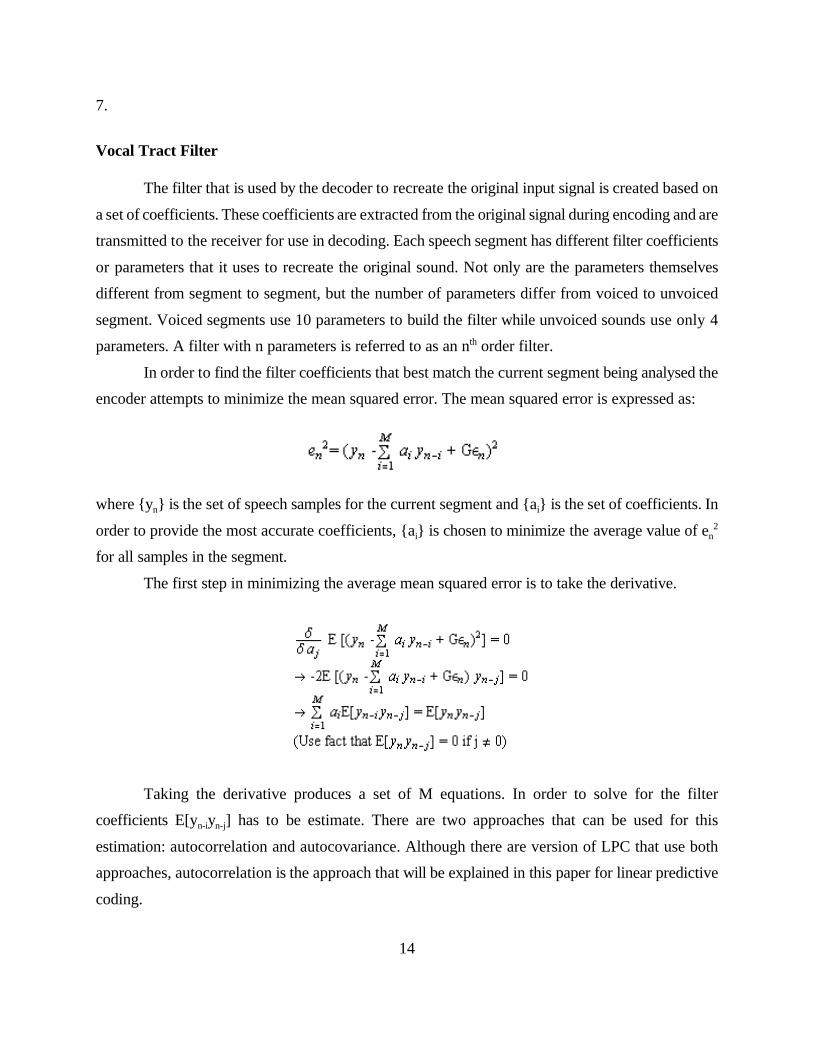
In order to find the filter coefficients that best match the current segment being analysed the

encoder attempts to minimize the mean squared error. The mean squared error is expressed as:

where {yn} is the set of speech samples for the current segment and {ai} is the set of coefficients. In

order to provide the most accurate coefficients, {ai} is chosen to minimize the average value of en2

for all samples in the segment.

The first step in minimizing the average mean squared error is to take the derivative.

Taking the derivative produces a set of M equations. In order to solve for the filter

coefficients E[yn-iyn-j] has to be estimate. There are two approaches that can be used for this

estimation: autocorrelation and autocovariance. Although there are version of LPC that use both

approaches, autocorrelation is the approach that will be explained in this paper for linear predictive

coding.

15

Autocorrelation requires that several initial assumptions be made about the set or sequence

of speech samples, {yn}, in the current segment. First, it requires that {yn} be stationary and second,

it requires that the {yn} sequence is zero outside of the current segment. In autocorrelation, each

E[yn-iyn-j] is converted into an autocorrelation function of the form Ryy(| i-j |). The estimation of an

autocorrelation function Ryy(k) can be expressed as:

Using Ryy(k), the M equations that were acquired from taking the derivative of the mean

squared error can be written in matrix form RA = P where A contains the filter coefficients.

In order to determine the contents of A, the filter coefficients, the equation A = R-1P must be solved.

This equation can not be solved with out first computing R-1. This is an easy computation if one

notices that R is symmetric and more importantly all diagonals consist of the same element. This type

of matrix is called a Toeplitz matrix and can be easily inverted.

The Levinson-Durbin (L-D) Algorithm is a recursive algorithm that is considered very

computationally efficient since it takes advantage of the properties of R when determining the filter

coefficients.. This algorithm is outlined in Figure 8 where the filter order is denoted with a

16

L-D Algorithm

Figure 8 : Levinson-Durbin (L-D) Algorithm for solving Toeplitz Matrices

superscript, {ai(j)}for a jth order filter, and the average mean squared error of a jth order filter is

denoted Ej instead of E[en2]. When applied to an Mth order filter, the L-D algorithm computes all

filters of order less than M. That is, it determines all order N filters where N=1,...,M-1.

During the process of computing the filter coefficients {ai} a set of coefficients, {ki}, called

reflection coefficients or partial correlation coefficients (PARCOR) are generated. These coefficients

are used to solve potential problems in transmitting the filter coefficients. The quantization of the

filter coefficients for transmission can create a major problem since errors in the filter coefficients can

lead to instability in the vocal tract filter and create an inaccurate output signal. This potential

problem is averted by quantizing and transmitting the reflection coefficients that are generated by the

Levinson-Durbin algorithm. These coefficients can be used to rebuild the set of filter coefficients {ai}

and can guarantee a stable filter if their magnitude is strictly less than one.

Transmitting the Parameters

In an uncompressed form, speech is usually transmitted at 64,000 bits/second using 8

bits/sample and a rate of 8 kHz for sampling. LPC reduces this rate to 2,400 bits/second by breaking

the speech into segments and then sending the voiced/unvoiced information, the pitch period, and the

coefficients for the filter that represents the vocal tract for each segment.

The input signal used by the filter on the receiver end is determined by the classification of the

17

speech segment as voiced or unvoiced and by the pitch period of the segment. The encoder sends a

single bit to tell if the current segment is voiced or unvoiced. The pitch period is quantized using a

log-companded quantizer to one of 60 possible values. 6 bits are required to represent the pitch

period.

If the segment contains voiced speech than a 10th order filter is used. This means that 11

values are needed: 10 reflection coefficients and the gain. If the segment contains unvoiced speech

than a 4th order filter is used. This means that 5 values are needed: 4 reflection coefficients and the

gain. The reflection coefficients are denote kn where 1 # n # 10 for voiced speech filters and 1 # n

# 4 for unvoiced filters.

The only problem with transmitting the vocal tract filter is that it is especially sensitive to

errors in reflection coefficients that have a magnitude close to one. The first few reflection

coefficients, k1 and k2, are the most likely coefficients to have magnitudes around one. To try and

eliminate this problem, LPC-10 uses nonuniform quantization for k1 and k2. First, each coefficient

is used to generate a new coefficient, gi, of the form:

These new coefficients, g1 and g2, are then quantized using a 5-bit uniform quantizer.

All of the rest of the reflection coefficients are quantized using uniform quantizers. k3 and k4

are quantized using 5-bit uniform quantization. For voiced segments k5 up to k8 are quantized using

4-bit uniform quantizers while k9 uses a 3-bit quantizer and k10 uses a 2-bit uniform quantizer. For

unvoiced segments the bits used in voiced segments to represent the reflection coefficients, k5 through

k10, are used for error protection. This means that unvoiced segments don’t omit the bits needed to

represent k5 up to k10 and therefore use the same amount of space as voiced segments. This also

means that the bit rate doesn’t decrease below 2,400 bits/second if a lot of unvoiced segments are

sent. Variation of bit rate is not good in the transmission of speech since most speech is transmitted

over shared lines where it is important to know how much of the line will be needed.

Once the reflection coefficients have been quantized the gain, G, is the only thing not yet

quantized. The gain is calculated using the root mean squared (rms) value of the current segment. The

gain is quantized using a 5-bit log-companded quantizer.

18

1 bit voiced/unvoiced6 bits pitch period (60 values)10 bits k1 and k2 (5 each)10 bits k3 and k4 (5 each)16 bits k5, k6, k7, k8 (4 each)3 bits k9

2 bits k10

5 bits gain G1 bit synchronization54 bits TOTAL BITS PER FRAME

Figure 9: Total Bits in each Speech Segment

Sample rate = 8000 samples/second

Samples per segment = 180 samples/segment

Segment rate = Sample Rate/ Samples per Segment= (8000 samples/second)/(180 samples/second)= 44.444444.... segments/second

Segment size = 54 bits/segment

Bit rate = Segment size * Segment rate= (54 bits/segment) * (44.44 segments/second)= 2400 bits/second

Figure 10: Verification for Bit Rate of LPC Speech Segments

The total number of bits required for

each segment or frame is 54 bits. This total is

explained in Figure 9. Recall that the input

speech is sampled at a rate of 8000 samples per

second and that the 8000 samples in each

second of speech signal are broken into 180

sample segments. This means that there are

approximately 44.4 frames or segments per

second and therefore the bit rate is 2400

bits/second as show in Figure 10.

7 LPC Synthesis/Decoding

The process of decoding a sequence of speech segments is the reverse of the encoding

process. Each segment is decoded individually and the sequence of reproduced sound segments is

joined together to represent the entire input speech signal. The decoding or synthesis of a speech

segment is based on the 54 bits of information that are transmitted from the encoder.

The speech signal is declared voiced or unvoiced based on the voiced/unvoiced determination

bit. The decoder needs to know what type of signal the segment contains in order to determine what

type of excitement signal will be given to the LPC filter. Unlike other speech compression algorithms

19

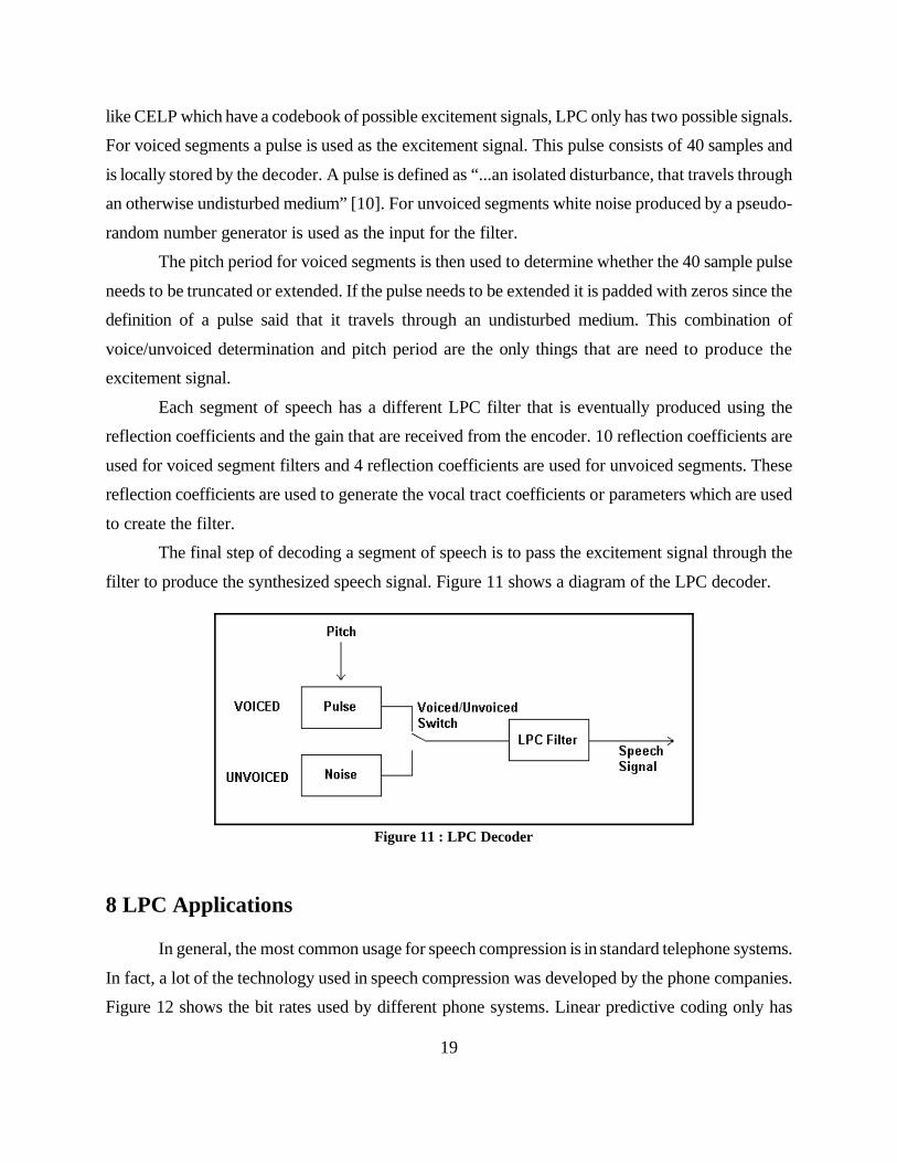
Figure 11 : LPC Decoder

like CELP which have a codebook of possible excitement signals, LPC only has two possible signals.

For voiced segments a pulse is used as the excitement signal. This pulse consists of 40 samples and

is locally stored by the decoder. A pulse is defined as “...an isolated disturbance, that travels through

an otherwise undisturbed medium” [10]. For unvoiced segments white noise produced by a pseudo-

random number generator is used as the input for the filter.

The pitch period for voiced segments is then used to determine whether the 40 sample pulse

needs to be truncated or extended. If the pulse needs to be extended it is padded with zeros since the

definition of a pulse said that it travels through an undisturbed medium. This combination of

voice/unvoiced determination and pitch period are the only things that are need to produce the

excitement signal.

Each segment of speech has a different LPC filter that is eventually produced using the

reflection coefficients and the gain that are received from the encoder. 10 reflection coefficients are

used for voiced segment filters and 4 reflection coefficients are used for unvoiced segments. These

reflection coefficients are used to generate the vocal tract coefficients or parameters which are used

to create the filter.

The final step of decoding a segment of speech is to pass the excitement signal through the

filter to produce the synthesized speech signal. Figure 11 shows a diagram of the LPC decoder.

8 LPC Applications

In general, the most common usage for speech compression is in standard telephone systems.

In fact, a lot of the technology used in speech compression was developed by the phone companies.

Figure 12 shows the bit rates used by different phone systems. Linear predictive coding only has

20

application in the area of secure telephony because of its low bit rate. Secure telephone systems

require a low bit rate since speech is first digitalized, then encrypted and transmitted. These systems

have a primary goal of decreasing the bit rate as much as possible while maintaining a level of

North American Telephone Systems 64 kb/s (uncompressed)

International Telephone Network 32 kb/s (can range from 5.3-64

kb/s)

Digital Cellular standards 6.7-13 kb/s

Regional Cellular standards 3.45-13 kb/s

Secure Telephony 0.8-16 kb/s

Figure 12 : Bit Rates for different telephone standards

speech quality that is understandable. Other standards such as the digital cellular standard and the

international telephone network standard have higher quality standards and therefore require a higher

bit rate. In these standards, understanding the speech is not good enough, the listener must also be

able to recognize the speech as belonging to the original source.

A second area that linear predictive coding has been used is in Text-to-Speech synthesis. In

this type of synthesis the speech has to be generated from text. Since LPC synthesis involves the

generation of speech based on a model of the vocal tract, it provides a perfect method for generating

speech from text.

Further applications of LPC and other speech compression schemes are voice mail systems,

telephone answering machines, and multimedia applications. Most multimedia applications, unlike

telephone applications, involve one-way communication and involve storing the data. An example of

a multimedia application that would involve speech is an application that allows voice annotations

about a text document to be saved with the document. The method of speech compression used in

multimedia applications depends on the desired speech quality and the limitations of storage space

for the application. Linear Predictive Coding provides a favourable method of speech compression

for multimedia applications since it provides the smallest storage space as a result of its low bit rate.

21

9 Conclusion

Linear Predictive Coding is an analysis/synthesis technique to lossy speech compression that

attempts to model the human production of sound instead of transmitting an estimate of the sound

wave. Linear predictive coding achieves a bit rate of 2400 bits/second which makes it ideal for use

in secure telephone systems. Secure telephone systems are more concerned that the content and

meaning of speech, rather than the quality of speech, be preserved. The trade off for LPC’s low bit

rate is that it does have some difficulty with certain sounds and it produces speech that sound

synthetic.

Linear predictive coding encoders break up a sound signal into different segments and then

send information on each segment to the decoder. The encoder send information on whether the

segment is voiced or unvoiced and the pitch period for voiced segment which is used to create an

excitment signal in the decoder. The encoder also sends information about the vocal tract which is

used to build a filter on the decoder side which when given the excitment signal as input can

reproduce the original speech.

22

10 References

[1] V. Hardman and O. Hodson. Internet/Mbone Audio (2000) 5-7.

[2] Scott C. Douglas. Introduction to Adaptive Filters, Digital Signal Processing Handbook(1999) 7-12.

[3] Poor, H. V., Looney, C. G., Marks II, R. J., Verdú, S., Thomas, J. A., Cover, T. M.Information Theory. The Electrical Engineering Handbook (2000) 56-57.

[4] R. Sproat, and J. Olive. Text-to-Speech Synthesis, Digital Signal Processing Handbook (1999)9-11 .

[5] Richard C. Dorf, et. al.. Broadcasting (2000) 44-47.

[6] Richard V. Cox. Speech Coding (1999) 5-8.

[7] Randy Goldberg and Lance Riek. A Practical Handbook of Speech Coders (1999) Chapter2:1-28, Chapter 4: 1-14, Chapter 9: 1-9, Chapter 10:1-18.

[8] Mark Nelson and Jean-Loup Gailly. Speech Compression, The Data Compression Book(1995) 289-319.

[9] Khalid Sayood. Introduction to Data Compression (2000) 497-509.

[10] Richard Wolfson, Jay Pasachoff. Physics for Scientists and Engineers (1995) 376-377.