Linear Prediction for Speech Encoding
102
Linear Prediction using Lattice Filters and its application in Speech Compression Abstract The project aims at studying the theory of Linear Prediction of Stationary Signals and using this knowledge in the application of compression of Speech. Linear Prediction can be achieved using a number of methods. We have used the Lattice Filter method of Linear Prediction and highlighted the advantages of this method. The calculation of p prediction coefficient involves the inversion of a P X P matrix. This involves O(p 3 ) operations. To reduce the number of operations we have used the Levinson Durbin algorithm which exploits a special property of the autocorrelation matrix to reduce the number of operations to O(p 2 ). To implement this technique on speech signal, we have segmented and windowed the speech samples in order to treat it as a stationary signal. We have analyzed the forward prediction error and the recreated signal on several criterion such as the order of prediction, size of the window segment and number of bits used to encode the error sequence. We have also created compressed sound files which can be heard to get an idea of the result obtained.
-
Upload
pricingcredit -
Category
Documents
-
view
217 -
download
0
Transcript of Linear Prediction for Speech Encoding

7/23/2019 Linear Prediction for Speech Encoding
http://slidepdf.com/reader/full/linear-prediction-for-speech-encoding 1/102
Linear Prediction using Lattice Filters
and its application in SpeechCompression
Abstract
The project aims at studying the theory of Linear Prediction of Stationary Signals and
using this knowledge in the application of compression of Speech. Linear Prediction can
be achieved using a number of methods. We have used the Lattice Filter method of Linear
Prediction and highlighted the advantages of this method. The calculation of p
prediction coefficient involves the inversion of a P X P matrix. This involves O(p3)
operations. To reduce the number of operations we have used the Levinson Durbin
algorithm which exploits a special property of the autocorrelation matrix to reduce the
number of operations to O(p2).
To implement this technique on speech signal, we have segmented and windowed the
speech samples in order to treat it as a stationary signal. We have analyzed the forward
prediction error and the recreated signal on several criterion such as the order of
prediction, size of the window segment and number of bits used to encode the error
sequence. We have also created compressed sound files which can be heard to get an
idea of the result obtained.

7/23/2019 Linear Prediction for Speech Encoding
http://slidepdf.com/reader/full/linear-prediction-for-speech-encoding 2/102
2
Contents
1. Introduction..................................................................................................................... 51.1 Human Speech Production........................................................................................ 5
1.2 Theory of Speech Coding ......................................................................................... 71.3 Historical Perspective of Linear Predictive Coding.................................................. 92. Linear Prediction........................................................................................................... 11
2.1 Innovations representation of a Random Process ................................................... 122.2 Rational Power Spectra........................................................................................... 142.3 Relationships between the Filter Parameters and the Autocorrelation Sequence... 16
2.4 Theory of linear Prediction..................................................................................... 18
2.4.1 The Autocorrelation Method............................................................................ 19
2.4.2 The Covariance Method................................................................................... 203. Lattice Filters ................................................................................................................ 24
3.1 Prediction Model Order Selection .......................................................................... 29
4. The Levinson-Durbin Algorithm................................................................................. 315. Progress Report............................................................................................................. 36
6. Observations and Results.............................................................................................. 44
6.1 Effect of order of prediction ................................................................................... 446.1.1 Spectrum of the Error Signal ........................................................................... 47
6.2 Effect of segment size............................................................................................. 54
6.3 Effect of quantisation and compression of error signal. ......................................... 56
7.1 Conclusions................................................................................................................. 647.2 Future Scope of the Project......................................................................................... 65
8. References..................................................................................................................... 66
A. Appendix I: New MATLAB Functions. ...................................................................... 68B. Appendix II: MATLAB Codes .................................................................................... 83
C. Appendix III C- Codes ............................................................................................. 90
Code C.1 Levinson Durbin Algorithm.......................................................................... 90Code C.2 Levinson Durbin Header File ....................................................................... 93
Code C.3 MA Lattice Filter .......................................................................................... 94
Code x.3 MA Lattice Filter Header File ....................................................................... 95
Code C.3 AR Lattice Filter ........................................................................................... 96Code C.3 AR Lattice Filter Header File ....................................................................... 98
Code C.3 Segmentation and Hanning Window............................................................ 99
Code C.3 Segmentation and Hanning Window Header File ...................................... 101

7/23/2019 Linear Prediction for Speech Encoding
http://slidepdf.com/reader/full/linear-prediction-for-speech-encoding 3/102
3
List of Figures
Figure 1.1: Human Speech Production System………………………………………… 8Figure 1.2: Model of Speech Production………………………………………………...9Figure 2.1: Time and Power Spectral Density Representation…………………………14
Figure 2.2: Filters for generating random process from white noise…………………...16Figure 3.1: Forward Linear Prediction………………………………………………… 27Figure 3.2: Prediction Error Filter……………………………………………………... 27
Figure 3.3: Single stage Lattice Filter…………………………………………………. 28
Figure 3.4: Two stage Lattice Filter…………………………………………………… 29
Figure 3.5: P stage Lattice Filter………………………………………………………. 30Figure 5.1: Original, Error and Recreated signal (without segmentation)…………….. 40
Figure 5.2: Original, Error and Recreated signal (with non-overlapping segmentation) 41
Figure 5.3: Original, Error and Recreated signal (with overlapping windowing)………42Figure 5.4: Original, Error and Recreated signal with lattice filters…………………… 43
Figure 5.5: Frequency Spectrum of Original Signal…………………………………… 44
Figure 5.6: Frequency Spectrum of Recreated Signal…………………………………. 45Figure 6.1: Graph of Prediction Gain Vs Order of Prediction…………………………..49
Figure 6.2: Frequency representation of error when order p=2……………………….. 50
Figure 6.3: Frequency representation of error when order p=6……………………….. 51
Figure 6.4: Frequency representation of error when order p=8. ……………………….52Figure 6.5: Frequency representation of error when order p=12……………………….52
Figure 6.6: Frequency representation of error when order p=20……………………… 52
Figure 6.7: Frequency representation of error when order p=40……………………… 53Figure 6.8: Frequency representation of original signal. ………………………………54
Figure 6.9: Frequency representation of original signal (Shifted)…………………….. 55
Figure 6.10: Frequency representation of recreated signal (Shifted) p=8………………56Figure 6.11: Frequency representation of recreated signal (Shifted) p=12……………. 56
Figure 6.12: Window size Vs Predictive Gain………………………………………… 58
Figure 6.13: Original Signal encoded in 8 bits………………………………………… 59
Figure 6.14: Recreated Signal when error is encoded in 8 bits………………………… 60Figure 6.15: Recreated Signal when error is encoded in 7 bits……………………….... 60
Figure 6.16: Recreated Signal when error is encoded in 6 bits………………………….61
Figure 6.17: Recreated Signal when error is encoded in 5 bits………………………… 61Figure 6.18: Recreated Signal when error is encoded in 4 bits………………………….62
Figure 6.19: Recreated Signal when error is encoded in 3 bits………………………….62
Figure 6.20: Recreated Signal Spectrum when error is encoded in 8 bits……………… 63Figure 6.21: Recreated Signal Spectrum when error is encoded in 7 bits……………….63
Figure 6.22: Recreated Signal Spectrum when error is encoded in 6 bits……………….64
Figure 6.23: Recreated Signal Spectrum when error is encoded in 5 bits……………… 64Figure 6.24: Recreated Signal Spectrum when error is encoded in 4 bits……………….65
Figure 6.25: Recreated Signal Spectrum when error is encoded in 3 bits……………… 65

7/23/2019 Linear Prediction for Speech Encoding
http://slidepdf.com/reader/full/linear-prediction-for-speech-encoding 4/102
4
Chapter 1
INTRODUCTION

7/23/2019 Linear Prediction for Speech Encoding
http://slidepdf.com/reader/full/linear-prediction-for-speech-encoding 5/102
5
1. Introduction
Linear prediction modelling is used in a diverse area of applications, such as data
forecasting, speech coding, video coding, speech recognition, model-based interpolation,signal restoration and impulse/step event detection. In our project we would be studying
and implementing linear predictive coding (lpc) for speech compression.
1.1 Human Speech Production
Regardless of the language spoken, all people use relatively the same anatomy to produce
sound. The output produced by each human’s anatomy is limited by the laws of physics.The process of speech production in humans can be summarized as air being pushed from
the lungs, through the vocal tract, and out through the mouth to generate speech. In this
type of description the lungs can be thought of as the source of the sound and the vocal
tract can be thought of as a filter that produces the various types of sounds that make up
speech. The above is a simplification of how sound is really produced.
Figure 1.1: Human Speech Production System.

7/23/2019 Linear Prediction for Speech Encoding
http://slidepdf.com/reader/full/linear-prediction-for-speech-encoding 6/102
6
Phonemes are defined as a limited set of individual sounds. There are two categories of
phonemes, voiced and unvoiced sounds. Voiced sounds are usually vowels and often
have high average energy levels and very distinct resonant or formant frequencies.
Voiced sounds are generated by air from the lungs being forced over the vocal cords. As
a result the vocal cords vibrate in a somewhat periodically pattern that produces a series
of air pulses called glottal pulses. The rate at which the vocal cords vibrate is what
determines the pitch of the sound produced. Unvoiced sounds are usually consonants and
generally have less energy and higher frequencies then voiced sounds. The production of
unvoiced sound involves air being forced through the vocal tract in a turbulent flow.
During this process the vocal cords do not vibrate, instead, they stay open until the sound
is produced.
The amount of air that originates in the lungs also affects the production of sound in
humans. The air flowing from the lungs can be thought of as the source for the vocal tract
which act as a filter by taking in the source and producing speech. The higher the volume
of air that goes through the vocal tract, the louder the sound.
Figure 1.2: Model of Speech Production.
Pitch period
Vocal Tract
Parameters
Impulse Train
Generator
Random Noise
Generator
Voiced / Unvoiced switch
X(n)Time-Varying
Digital Filter
G

7/23/2019 Linear Prediction for Speech Encoding
http://slidepdf.com/reader/full/linear-prediction-for-speech-encoding 7/102
7
Some of the fundamental properties of the speech signal that can be successfully
exploited for compression of speech include the quasi-stationary nature of the speech
signal. Quasi-stationary means that speech can be treated as a stationary signal for short
intervals of time. This allows us to use techniques which are generally used for stationary
signals for processing speech signals. The amplitude of speech signal varies slowly with
time, which is another characteristic that is commonly exploited for compression
purpose.
1.2 Theory of Speech Coding
The recent exponential growth of telecommunications today drives all aspects of
technology to higher degrees than ever before, creating the need to transfer maximal
amount of information consuming minimal relevant resources. Due to the impact on
parameters such as bandwidth requirements and conversation quality, the most important
component of any telephony system is that which generates the digital representation of
the speech.
Linear Predictive Coding (LPC) is defined as a digital method for encoding an analog
signal in which a particular value is predicted by a linear function of the past values of
the signal. It was first proposed as a method for encoding human speech by the United
States Department of Defense in federal standard 1015, published in 1984.
There exist many different types of speech compression that make use of a variety of
different techniques. However, most methods of speech compression exploit the fact that
speech production occurs through slow anatomical movements and that the speech
produced has a limited frequency range. The frequency of human speech productionranges from around 300 Hz to 3400 Hz. Speech compression is often referred to as
speech coding which is defined as a method for reducing the amount of information
needed to represent a speech signal. There are many other characteristics about speech
production that can be exploited by speech coding algorithms. One fact that is often used
is that period of silence take up greater than 50% of conversations. An easy way to save

7/23/2019 Linear Prediction for Speech Encoding
http://slidepdf.com/reader/full/linear-prediction-for-speech-encoding 8/102
8
bandwidth and reduce the amount of information needed to represent the speech signal is
to not transmit the silence. Another fact about speech production that can be taken
advantage of is that mechanically there is a high correlation between adjacent samples of
speech. Most forms of speech compression are achieved by modeling the process of
speech production as a linear digital filter. The digital filter and its slow changing
parameters are usually encoded to achieve compression from the speech signal.
Any signal processing system that aims to achieve utmost economy in the digital
representation of speech for storage or transmission must be based on the physical
constraints of our speech production apparatus and must exploit the limitations of human
hearing. It is wasteful to reserve costly bits for signals that the human mouth (and nose)
can never emit; it is equally wasteful to represent signal differences in the encoded bit
stream that the human ear can never distinguish.
Speech coding or compression is usually conducted with the use of voice coders or
vocoders. There are two types of voice coders: waveform-following coders and model-
base coders. Waveform following coders will exactly reproduce the original speech
signal if no quantization errors occur. Model-based coders will never exactly reproduce
the original speech signal, regardless of the presence of quantization errors, because they
use a parametric model of speech production which involves encoding and transmitting
the parameters not the signal. LPC vocoders are considered model-based coders which
mean that LPC coding is lossy even if no quantization errors occur.
The general algorithm for linear predictive coding involves an analysis or encoding part
and a synthesis or decoding part. In the encoding, LPC takes the speech signal in blocks
or frames of speech and determines the input signal and the coefficients of the filter that
will be capable of reproducing the current block of speech. This information is quantized
and transmitted. In the decoding, LPC rebuilds the filter based on the coefficients
received. The filter can be thought of as a tube which, when given an input signal,
attempts to output speech. Additional information about the original speech signal is used

7/23/2019 Linear Prediction for Speech Encoding
http://slidepdf.com/reader/full/linear-prediction-for-speech-encoding 9/102
9
by the decoder to determine the input or excitation signal that is sent to the filter for
synthesis.
1.3 Historical Perspective of Linear Predictive Coding
The history of audio and music compression begin in the 1930s with research into pulse-
code modulation (PCM) and PCM coding. Compression of digital audio was started in
the 1960s by telephone companies who were concerned with the cost of transmission
bandwidth. Linear Predictive Coding’s origins begin in the 1970s with the development
of the first LPC algorithms. Adaptive Differential Pulse Code Modulation (ADPCM),
another method of speech coding, was also first conceived in the 1970s.
The history of speech coding makes no mention of LPC until the 1970s. However, the
history of speech synthesis shows that the beginnings of Linear Predictive Coding
occurred 40 years earlier in the late 1930s. The first vocoder was described by Homer
Dudley in 1939 at Bell Laboratories. Dudley developed his vocoder, called the Parallel
Bandpass Vocoder or channel vocoder, to do speech analysis and re-synthesis. LPC is a
descendent of this channel vocoder. The analysis/synthesis scheme used by Dudley is the
scheme of compression that is used in many types of speech compression such as LPC.
The idea of using LPC for speech compression came up in 1966 when Manfred R.
Schroeder and B.S. Atal turned their attention to the following: for television pictures, the
encoding of each picture element (“pixel”) as if it was completely unpredictable is of
course rather wasteful, because adjacent pixels are correlated. Similarly, for voiced
speech, each sample is known to be highly correlated with the corresponding sample that
occurred one pitch period earlier. In addition, each sample is correlated with the
immediately preceding samples because the resonances of the vocal tract. Therefore short
durations of speech show an appreciable correlation.

7/23/2019 Linear Prediction for Speech Encoding
http://slidepdf.com/reader/full/linear-prediction-for-speech-encoding 10/102
10
Chapter 2
LINEAR PREDICTION

7/23/2019 Linear Prediction for Speech Encoding
http://slidepdf.com/reader/full/linear-prediction-for-speech-encoding 11/102
11
2. Linear Prediction
The success with which a signal can be predicted from its past samples depends on the
autocorrelation function, or equivalently the bandwidth and the power spectrum, of the
signal. As illustrated in figure 2.1, in the time domain, a predictable signal has a smooth
and correlated fluctuation, and in the frequency domain, the energy of a predictable
signal is concentrated in narrow band/s of frequencies. In contrast, the energy of an
unpredictable signal, such as white noise, is spread over a wide band of frequencies.
Figure 2.1: Time and Power Spectral Density Representation.
For a signal to have a capacity to convey information it must have a degree of
randomness. Most signals, such as speech, music and video signals are, partially
predictable and partially random. These signals can be modeled as the output of a filter
excited by an uncorrelated input. The random input models the unpredictable part of the
signal, whereas the filter models the predictable structure of the signal. The aim of linear
prediction is to model the mechanism that introduces the correlation in a signal.

7/23/2019 Linear Prediction for Speech Encoding
http://slidepdf.com/reader/full/linear-prediction-for-speech-encoding 12/102
12
2.1 Innovations representation of a Random Process
A wide sense stationary random process may be represented as the output of a causal and
causally invertible linear system excited by a white noise process. The condition that the
system is causally invertible also allows us to represent the wide sense stationary random
process by the output of the inverse system, which is a white process. This statement is
explained below.
Let us consider a wide-sense stationary process x(n) with the autocorrelation sequence
)(m xxγ and power spectral density )( f xxΓ , | f | <=1/2. The z-transform of the
autocorrelation sequence )(m xxγ is
∑∞
−∞=
−=Γ
m
m
xx xx zm z )()( γ 2.1
from which we obtain the power spectral density by evaluating )( z xxΓ on the unit
circle(that is by substituting z=exp( j2*pi*f) )
Assuming that log )( z xxΓ is analytic (possesses derivatives of all orders) in an annular
region in the z-plane that include the unit circle. Then log )( z xxΓ may be expanded in a
Laurent series of the form, for z=exp( j2*pi*f).
∑∞
−∞=
−=Γ
m
fm j
xx emv f π 2)()(log 2.2
where v(m) are the coefficients in the series expansion. Further, v(m) may be viewed as
the sequence with z transform V(z)= log )( z xxΓ . Thus,
=Γ ∑
∞
−∞=
−
m
m
xx zmv z )(exp)( 2.3
)()(12 −
= z H z H wσ

7/23/2019 Linear Prediction for Speech Encoding
http://slidepdf.com/reader/full/linear-prediction-for-speech-encoding 13/102
13
where by definition2
wσ =exp[v(0)]
and 1
1
,)(exp)( r z zmv z H m
m>
= ∑
∞
−=
−
On evaluating the above equation on the unit circle, we have the equivalent
representation of the power spectral density as
22)()( f H f w xx σ =Γ 2.4
The filter with the system function H(z) is analytic in the region | z|>r1<1. Hence in this
region it has a Talyor series expansion as a causal system of the form
n
m
znh z H −
∞
=
∑=
0
)()( 2.5
The output of this filter to a white noise input sequence w(n) with power spectral density
2
wσ is a stationary random process x(n) with power spectral density22
)()( f H f w xx σ =Γ .
Conversely, the stationary random process x(n) with the power spectral density2
wσ may
be transformed into a white noise process by passing x(n) through a linear filter with
system function 1/ H(z) This filter is called a noise whitening filter . Its output, denoted as
w(n) is called the innovations process associated with the stationary random process x(n).
Figure 2.2: Filters for generating random process from white noise and the
inverse filter.
w(n)
∑∞
=
−=
0
)()()(k
k nwk hn x
White noise
x(n)
w(n)
White noise
Linear causal
filter, H(z)
Linear causal
filter, 1/ H(z)

7/23/2019 Linear Prediction for Speech Encoding
http://slidepdf.com/reader/full/linear-prediction-for-speech-encoding 14/102
14
2.2 Rational Power Spectra
Considering the power spectral density of the stationary random process x(n) is a rational
function, expressed as
,)()(
)()()(
1
12
−
−
=Γ z A z A
z B z B z w xx σ 21 r zr << 2.6
Where the polynomials B(z) and A(z) have roots that fall inside the unit circle in the z-
plane. Then the linear filter H(z) for generating the random process x(n) from the white
noise sequence w(n) is also rational and is expressed as
,
1)(
)()(
1
0
∑
∑
=
−
=
−
+
== p
k
k
k
q
k
k
k
za
zb
z A
z B z H 1r z > 2.7
where bk and ak are the filter coefficients that determine the location of the zeros and
poles of H(z), respectively. Thus H(z) is causal, stable, and minimum phase. Its
reciprocal 1/H(z) is also a causal, stable, and minimum phase linear system. Therefore the
random process x(n) uniquely represents the statistical properties of the innovation
process w(n), and vice versa.
For the linear system with the rational system function H(z) given by above equation, the
output x(n) is related to the input w(n) by the following difference equation
∑∑==
−=−+q
k
k
p
k
k k nwbk n xan x01
)()()( 2.8

7/23/2019 Linear Prediction for Speech Encoding
http://slidepdf.com/reader/full/linear-prediction-for-speech-encoding 15/102
15
Distinguishing among three special cases:
Autoregressive (AR) Process: b0 = 1, bk = 0, k > 0
In this case the linear filter H(z) = 1/A(z) is an all-pole filter and the difference equation
for the input-output relationship is
)()()(1
nwk n xan x p
k
k =−+∑=
2.9
In turn, the noise-whitening filter for generating the innovations process is an all zero
filter.
Moving Average (MA) process : ak = 0, k >= 1
In this case the linear filter H(z) = B(z) is an all-zero filter and the difference equation for
the input-output relationship is
∑=
−=
q
k
k k nwbn x0
)()( 2.10
The noise-whitening filter for generating the innovations process is an all pole filter.
Autoregressive, Moving Average (ARMA) Process : In this case the linear filter
H(z) = B(z)/A(z) has both poles and zeros in the z-plane and the corresponding difference
equation is given by 2.8. The inverse system for generating the innovations process w(n)
from x(n) is also a pole-zero system of the form 1/H(z) = A(z)/B(z).

7/23/2019 Linear Prediction for Speech Encoding
http://slidepdf.com/reader/full/linear-prediction-for-speech-encoding 16/102
16
2.3 Relationships between the Filter Parameters and the Autocorrelation Sequence
When the power spectral density of the stationary random process is a rational function,
there is a basic relationship that exists between the autocorrelation sequence)(m xxγ
and
the parameters ak and bk of the linear filter H(z) that generates the process by filtering the
white noise sequence w(n). This relationship may be obtained by multiplying the
difference equation in 2.8 by x*(n-m) and taking the expected value of the both sides of
the resulting equation, to get
∑∑==
−+−−=q
k
wxk
p
k
xxk xx k mbk mam01
)()()( γ γ γ
2.11
where)(mwxγ
is the cross-correlation sequence between w(n) and x(n).
The cross-correlation sequence)(mwxγ
is related to the filter impulse response, as shown
below
)()()(*
mnwn x E mwx +=γ
+−= ∑
∞
=
)()()(0
*mnwk nwk h E
k 2.12
)(2 mhw −= σ
where in the last step, it was assumed that the sequence w(n) is white.
From 2.12 the following relationship is obtained:

7/23/2019 Linear Prediction for Speech Encoding
http://slidepdf.com/reader/full/linear-prediction-for-speech-encoding 17/102
17
<−
≤≤+−−
>−−
= ∑ ∑
∑
=
−
=
+
=
0),(
0,)()(
),(
)(
*
1 0
2
1
mm
qmbk hk ma
qmk ma
m
xx
p
k
mq
k
mk w xxk
p
k
xxk
xx
γ
σ γ
γ
γ
2.13
This represents a nonlinear relationship between)(m xxγ
and the parameters ak and bk.
The relationship in 2.13 applies, in general, to the ARMA process. For an AR process,
2.13simplifies to
<−
=+−−
>−−
= ∑
∑
=
=
0),(
0,)(
0),(
)(
*
1
2
1
mm
mk ma
mk ma
m
xx
p
k
w xxk
p
k
xxk
xx
γ
σ γ
γ
γ
2.14
Thus a linear relationship is obtained between)(m xxγ
and the parameters ak
and bk .
These equations are called the Yule-Walker equations and may be expressed in the matrix
form
=
−−
−
−
0
....
0
0
....
1
)0(........)2()1(
........................
)2(........)0()1(
)1(........)1()0(
2
2
*
** w
p
xx xx xx
xx xx xx
xx xx xx
a
a
a
p p
p
pσ
γ γ γ
γ γ γ
γ γ γ
2.15
This correlation matrix is Toeplitz and hence it can be efficiently inverted by the use of
Levinson-Durbin algorithm as shown later.

7/23/2019 Linear Prediction for Speech Encoding
http://slidepdf.com/reader/full/linear-prediction-for-speech-encoding 18/102
18
2.4 Theory of linear Prediction
Linear prediction involves predicting the future values of a stationary random process
from the observation of past values of the process. Consider, in particular, a one step
forward linear predictor, which forms the prediction of the value x(n) by a weighted
linear combination of the past values x(n-1),x(n-2) ... x(n-p).
Hence linearly predicted value of x(n) is
)(^
n x = - )()(1
k n xk a pk
k
p −∑=
=
2.16
Where the –ap(k) represent the weights in the linear combination. These weights are
called prediction coefficients of the one step forward linear predictor of order P. The
negative sign in the definition of x(n) is for mathematical convenience.
The difference between the value x(n) and the predicted value )(^
n x is called the forward
prediction error, denoted by f p(n) ,
)()()(^
n xn xn f p
−= = )(n x + )()(1
k n xk a pk
k
p −∑=
=
2.17
For information bearing signals, the prediction error f p(n) may be regarded as the
information, or the innovation, content of the sample.
To calculate the optimum prediction coefficients for our prediction filter we minimize the
mean square error i.e.
Σ ( )()(^
n xn x − )2
is minimum.

7/23/2019 Linear Prediction for Speech Encoding
http://slidepdf.com/reader/full/linear-prediction-for-speech-encoding 19/102
19
Two approaches can obtain the LPC coefficients ak characterizing an all-pole H(z) model.
The least mean square method selects ak to minimize the mean energy in e(n) over a
frame of signal data, while the lattice filter approach permits instantaneous updating of
the coefficients.
The first of the two common least squares technique is the autocorrelation method,
which multiplies the speech signal by a window w(n) so that x’(n)=w(n)x(n) has a finite
duration.
The autocorrelation sequence rss describes the redundancy in the signal x(n).
2.18
where x(n), n = {-P, (-P) + 1, . . . ,N - 1} are the known samples and the
N is a normalizing factor.
2.4.1 The Autocorrelation Method
In this method, the speech segment is assumed zero outside the interval .10 −≤≤ N m
Thus the Speech Sample can be expressed as
( )( ) ( )
−≤≤+
=otherwise
N mmwnm xm xn
,0
10,.
2.19
Another least square technique called covariance method windows the error signal,
instead of the actual speech signal.

7/23/2019 Linear Prediction for Speech Encoding
http://slidepdf.com/reader/full/linear-prediction-for-speech-encoding 20/102
20
Autocovariance measures the redundancy in a signal
2.20
2.4.2 The Covariance Method
An alternative to using a weighting function or window for defining xn(m) is to fix the
interval over which the mean squared error is computed to the range 10 −≤≤ N m
And use the unweighted speech directly. That is
( )me E N
nn ∑−
=
1
0
2
where( )k in ,φ
is defined as
( ) ( ) ( )∑−
=
−−=
1
0
,, N
m
nnn k m xim xk iφ
pk
pi
≤≤
≤≤
0
1
2.21
or by a change of variable
( ) ( ) ( )∑ −+= k im xm xk i nnn ,φ
pk
pi
≤≤
≤≤
0
1
2.22
Using the extended speech interval to define the covariance values, ( )k i,φ , the matrix
form of the LPC analysis equation becomes,

7/23/2019 Linear Prediction for Speech Encoding
http://slidepdf.com/reader/full/linear-prediction-for-speech-encoding 21/102
21
( ) ( ) ( )
( ) ( ) ( )
( ) ( ) ( )
( )
( )
( )
=
p,0
:
2,0
1,0
:
pp,.........p,2p,1
:.........::
p2,.........2,22,1
p1,.........1,21,1
2
1
φ
φ
φ
φ φ φ
φ φ φ
φ φ φ
pa
a
a
2..23
The resulting covariance matrix is symmetric (since( ) ( )ik k i nn ,, φ φ =
) but not Toeplitz,
and can be solved efficiently be a set of techniques called the Cholesky decomposition.
The mean-square value of the forward linear prediction error f p(n) based on the
autocorrelation method is
∑ ∑∑= = =
−++==
p
k
p
k
p
l
xx p p xx p xx p
f
p k lk alak k an f E 1 1 1
**2 )()()()]()(Re[2)0(]|)([| γ γ γ ε 2.24
Now, f
pε is a quadratic function of the predictor coefficients, and its minimization leads
to the set of linear equations
)(l xxγ = - plk lk a p
k
xx p ,......,2,1.....,.........)()(1
=−∑=
γ 2.25
These are called the normal equations for the coefficients of the linear predictor. The
minimum mean-square prediction error is thus :
)()()0(]min[
1
k k a E xx
p
k
p xx
f
p
f
p −+=≡ ∑=
γ γ ε 2.26
Writing eq 2.26 in terms of vectors
xx xx r R =pa f 2.27

7/23/2019 Linear Prediction for Speech Encoding
http://slidepdf.com/reader/full/linear-prediction-for-speech-encoding 22/102
22
or which the predictor coefficients can be obtained as
xx xx r R1
p )(a −= 2.28
A question may arise as to whether to use the autocorrelation method or the covariance
method in estimating the predictor parameters. The covariance method is quite general
and can be used with no restrictions. The only problem is that of stability of the resulting
filter. In the autocorrelation method on the other hand, the filter is guaranteed to be
stable, but problems of the parameter accuracy can arise because of the necessity of the
windowing (truncating) the rime signal. This is usually a problem if the signal is a portion
of an impulse response. For example, if the impulse response of an all-pole filter is
analyzed by covariance method, the filter parameters can be computed accurately from
only a finite number of samples of the signal. Using the autocorrelation method, one can
not obtain the exact parameters values unless the whole infinite impulse response is used
in the analysis. However, in practice, very good approximations can be obtained by
truncating the impulse response at a point where most of the decay of the response has
already occurred.

7/23/2019 Linear Prediction for Speech Encoding
http://slidepdf.com/reader/full/linear-prediction-for-speech-encoding 23/102
23
Chapter 3
LATTICE FILTERS

7/23/2019 Linear Prediction for Speech Encoding
http://slidepdf.com/reader/full/linear-prediction-for-speech-encoding 24/102
24
3. Lattice Filters
Linear prediction can be viewed as being equivalent to linear filtering where the predictor
is embedded in the linear filter, as shown in figure 3.1.
Figure 3.1: Forward Linear Prediction.
This is called a prediction-error filter with the input sequence x(n) and the output
sequence f p(n). An equivalent realization for the prediction-error filter is shown in fig 3.2
Figure 3.2: Prediction Error Filter.
x(n) p(n)
_
+
)(^
n x x(n-1)z
-1
Forward
Linear
Predictor
f p(n)
x(n)
a p(p)a p(p-1)a p(3)a p(2)a p(1)1
-1 -1 -1 -1

7/23/2019 Linear Prediction for Speech Encoding
http://slidepdf.com/reader/full/linear-prediction-for-speech-encoding 25/102
25
This realization is a direct-form FIR filter with the system function given as
∑=
−=
p
k
k
p p zk a z A0
)()( 3.1
where, by definition, a p(0) = 1.
Prediction Error filters can be realised in other way also, which take the form of a lattice
structure. To find a relationship between the Lattice filter coefficients and the FIR filter
structure, let us begin with a predictor of order p=1. The output of such a filter is
)1()1()()( 11 −+= n xan xn f 3.2
This output can be obtained from the single stage lattice filter, as shown in figure 3.3
below, by exciting both the inputs by x(n) and selecting the output from the top branch.
Figure 3.3: Single stage Lattice Filter.
Thus the output is exactly that given by above equation if we select K 1 = a1(1). The
parameter K 1 in the lattice filter is called a reflection coefficient.
The negated reflection coefficient, - k m , is also called the partial correlation (PARCOR)
coefficient
f 0(n)
g0(n-1)g0(n) g1(n)
f 1(n)
K *
K
-1
x n
7/23/2019 Linear Prediction for Speech Encoding
http://slidepdf.com/reader/full/linear-prediction-for-speech-encoding 26/102
26
Next, considering a predictor of order p = 2. For this case, the output of the direct-form
FIR filter is :
)2()2()1()1()()( 222 −+−+= n xan xan xn f 3.3
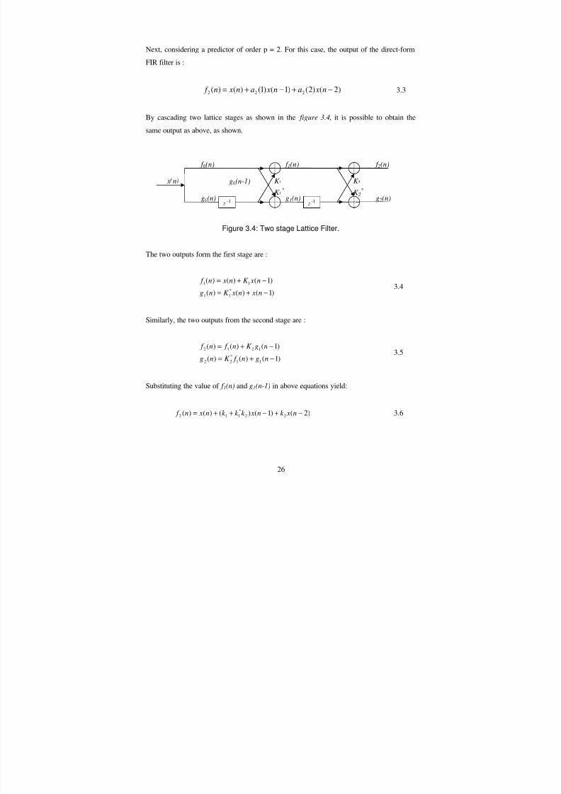
By cascading two lattice stages as shown in the figure 3.4, it is possible to obtain the
same output as above, as shown.
Figure 3.4: Two stage Lattice Filter.
The two outputs form the first stage are :
)1()()(
)1()()(
*
11
11
−+=
−+=
n xn xK ng
n xK n xn f
3.4
Similarly, the two outputs from the second stage are :
)1()()(
)1()()(
11
*
22
1212
−+=
−+=
ngn f K ng
ngK n f n f 3.5
Substituting the value of f 1(n) and g1(n-1) in above equations yield:
)2()1()()()( 22
*
112 −+−++= n xk n xk k k n xn f 3.6
g2(n)
f 2(n)
K 2*
K
f 0(n)
g0(n-1)
g0(n) g1(n)
f 1(n)
K *
K
-1
x n
-1

7/23/2019 Linear Prediction for Speech Encoding
http://slidepdf.com/reader/full/linear-prediction-for-speech-encoding 27/102
27
On equating coefficients we get,
a2(2)=K 2 and a2(1)= )( 2
*
11 k k k + 3.7
or equivalently,
K 2 = a2(2), K 1 = a1(1) 3.8
By continuing this process, the equivalence between an mth
order direct-form FIR filter
and an mth stage lattice filter can be demonstrated. The lattice is described by the
following set of order-recursive equations:
)1()()(
)1()()(
)()()(
11
*
11
00
−+=
−+=
==
−−
−−
ngn f K ng
ngK n f n f
n xngn f
mmmm
mmmm
pm
pm
,......,2,1
,......,2,1
=
=
3.9
A p-stage lattice filter for pth
order predictor can be shown as follows :
Figure 3.5: P stage Lattice Filter.
As a consequence of the equivalence between the direct form prediction error filter and
the FIR lattice filter, the output of the p-stage lattice filter is expressed as :
∑=
=−=
p
k
p p p ak n xk an f 0
1)0(.....................),........()()( 3.10
g p(n)
f p(n)
g2(n)
f 2(n)
g1(n)
f 1(n)
g0(n)
f 0(n)
First
Stage
Second
Stage
pth
Stage

7/23/2019 Linear Prediction for Speech Encoding
http://slidepdf.com/reader/full/linear-prediction-for-speech-encoding 28/102
28
The lattice forms characterization requires only p reflection coefficients Ki for a p step
linear predictor in comparison with the p(p+1)/2 filter coefficients required by the FIR
filter implementation. The reason that the lattice provides a more compact representation
is because appending stages to the lattice does not alter the parameters of the previous
stages. On the other hand, appending the pth
stage to a FIR based predictor results in
system function A p(z) that has coefficients totally different from the coefficients of the
lower-order FIR filter with system function A p-1(z).
Although the direct-form implementation of the linear predictor is the most convenient
method, for many applications, such as transmission of the predictor coefficients in
speech coding, it is advantageous to use the lattice form of predictor. This is because the
lattice form can be conveniently checked for stability. That is, for a stable model, the
magnitude of reflection coefficient is bounded by unity, and therefore it is relatively easy
to check a lattice structure for stability.
The quantization of the filter coefficients for transmission can create a major problem
since errors in the filter coefficients can lead to instability in the vocal tract filter and
create an inaccurate output signal. This potential problem is averted by quantizing and
transmitting the reflection coefficients that are generated by the Levinson-Durbin
algorithm. These coefficients can be used to rebuild the set of filter coefficients {a i} and
can guarantee a stable filter if their magnitude is strictly less than one.
A major attraction of a lattice structure is its modular form and the relative ease with
which the model order can be extended. Furthermore a perturbation of the parameter of
any section of the lattice structure has a limited and more localized effect.

7/23/2019 Linear Prediction for Speech Encoding
http://slidepdf.com/reader/full/linear-prediction-for-speech-encoding 29/102
29
3.1 Predictor Model Order Selection
One procedure for the determination of the correct model order is to increment the model
order, and monitor the differential change in the error power, until the change levels off.
The incremental change in error power with the increasing model order from i-1 to I is
defined as
)()1()( iii E E E −=∆− 3.11
The order p beyond which the decrease in the error power becomes less than a threshold
is taken as the model order.
When the model order is less than the correct order, the signal is under-modelled. In this
case, the prediction error is not well decorrelated and will be more than the optima;
minimum. A further consequence of the under-modelling is a decrease in the spectral
resolution of the model: adjacent spectral peaks of the signal could be merged and appear
as a single spectral peak when the model order is too small. When the model order is
larger than the correct order, the signal is over-modelled. An over-modelled problem can
result in an ill-conditioned matrix equation, unreliable numerical solutions and the
appearance of spurious spectral peaks in the model.

7/23/2019 Linear Prediction for Speech Encoding
http://slidepdf.com/reader/full/linear-prediction-for-speech-encoding 30/102
30
Chapter 4
Levinson Durbin Algorithm

7/23/2019 Linear Prediction for Speech Encoding
http://slidepdf.com/reader/full/linear-prediction-for-speech-encoding 31/102
31
4. The Levinson-Durbin Algorithm
The Levinson Durbin algorithm is a computationally efficient algorithm for solving the
normal equations. It is named so in recognition of its first use by Levinson(1947) and
then its independent reformulation at a later date by Durbin(1960).
,0)()(0
=−∑=
k lk a xx
p
k
p γ l=1, 2, ………………, p, ap(0)=1 4.1
for the prediction coefficients. This algorithm exploits the special symmetry in the
autocorrelation matrix
−−
−
−
=Γ
)0(........)2()1(
........................
)2(........)0()1(
)1(........)1()0(*
**
xx xx xx
xx xx xx
xx xx xx
p
p p
p
p
γ γ γ
γ γ γ
γ γ γ
4.2
Since )(),( ji ji
p p−Γ =Γ
, so the autocorrelation matrix is aToeplitz matrix
. Also, since
),(),( * ji ji p p Γ =Γ , the matrix is also Hermitian.
The key to the Levinson Durbin method of solution that exploits the Toeplitz property of
the matrix is to proceed recursively, beginning with a predictor of the order m=1 (one
coefficient) and to increase the order recursively, using the lower order solutions to
obtain the solution to the next higher order. Thus the solution to the first order predictor
obtained by solving the equation is
)0( / )1()1(1 xx xxa γ γ −= 4.3
and the resulting minimum mean square error (MMSE) is

7/23/2019 Linear Prediction for Speech Encoding
http://slidepdf.com/reader/full/linear-prediction-for-speech-encoding 32/102
32
]|)1(|1)[0( 2
11 a E xx
f −= γ 4.4
The next step is to solve for the coefficients a2(1) and a2(2) of the second order predictorand express the solution in terns of a1(1). The resulting equations are
)2()0()2()1()1(
)1()1()2()0()1(
22
*
22
xx xx xx
xx xx xx
aa
aa
γ γ γ
γ γ γ
−=+
−=+4.5
By using the solution in 4.4 to eliminate )1( xxγ , the following equations are obtained
])1(1)[0(
)2()1()1()2(
2
1
1
2
a
aa
xx
xx xx
−
+−=
γ
γ γ 4.6
f
xx xx
E
a
1
1 )2()1()1( γ γ +−=
)1()2()1()1( *
1212 aaaa += 4.7
In this manner to represent in terms of a recursive equation we express the coefficients of the mth order predictor in terms of the coefficients of the (m-1)st order predictor, We can
write the coefficient vector am as the sum of two vectors, namely
+
=
=
−−
m
mm
m
m
m
m
m
K
d a
ma
a
a
a
...
0
...
)(
....
)3(
)2(
)1( 11
a 4.8
where am-1 is the predictor coefficient vector of the (m-1)st order predictor and the vector
dm-1 and the scalar Km are the scalar Km are to be determined. For this the m X m
autocorrelation matrix xxΓ as

7/23/2019 Linear Prediction for Speech Encoding
http://slidepdf.com/reader/full/linear-prediction-for-speech-encoding 33/102
33
Γ =Γ
−
−−
)0(1
*
11
xx
bt
m
mm
mγ γ
γ 4.9
where [ ] ( )t b
m xx xx xx
bt
m mm 11 )1(.......)2()1(−−
=−−= γ γ γ γ γ .The superscript b on 1−mγ
denotes the vector [ ])1(.......)2()1(1 −=−
m xx xx xx
bt
m γ γ γ γ with elements taken in
reverse order.
The solution to the equation mmm a γ −=Γ may be expressed as
−=
+
Γ −−−
−
−−
)(0)0(
111
1
*
11
mK
d a
xx
m
m
mm
xxbt m
mm
γ
γ
γ γ
γ 4.10
This is the key step in the Levinson Durbin algorithm. From 4.10, two equations are
obtained as follows
1
*
11111 −−−−−−−=+Γ +Γ m
b
mmmmmm K d a γ γ 4.11
)()0(11111 mK d a xx xxmm
bt
mm
bt
m γ γ γ γ −=++−−−−
4.12
Since 111 −−−−=Γ mmm a γ , 4.11 yields the solution
*
1
1
11
b
mmmm K d −
−
−−Γ −= γ
−
−
==
−
−
−
−−
)1(
...
)2(
)1(
*1
*
1
*
1
*
11
m
m
m
m
b
mmm
a
ma
ma
K aK d 4.13
The scalar equation 4.12 can be used to solve for K m

7/23/2019 Linear Prediction for Speech Encoding
http://slidepdf.com/reader/full/linear-prediction-for-speech-encoding 34/102
34
( )
( ) *
11
11
0−−
−−+
−=
m
bt
m xx
m
bt
m xx
ma
amK
γ γ
γ γ 4.14
Thus substituting the solutions in 4.13 and 4.14 into 4.8, we get the recursive equations
for the predictor coefficients and the reflection coefficients for the lattice filters. The
recursive equations are given as
( )( )
( )
( )
( ) ( )
( ) ( ) ( ) )(
)(
0
*
11
*
11
11
*
11
11
k mamak ak a
k maK k ak a
E
am
a
amK ma
mmmm
mmmm
f
m
m
bt
m xx
m
bt
m xx
m
bt
m xx
mm
−+=
−+=
+−=
+−==
−−
−−
−−
−−
−−γ γ
γ γ
γ γ
4.15
From the equations we note that the predictor coefficients form a recursive set of
equations. Km is the reflection of the mth
stage. Also Km=am(m), the mth coefficient of
the mth
stage.
The important virtue of the Levinson-Durbin algorithm is its computational efficiency, in
that its use results in a big saving in the number of operations. The Levinson-Durbinrecursion algorithm requires O(m) multiplications and additions(operations) to go from
stage m to stage m+1. Therefore, for p stages it will take on the order of 1+2+3+…+p =
p(p+1)/2, or O(p2) operations to solve for the prediction filter coefficients or the
reflection coefficients, compared with O(p3) operations if the Toeplitz property is not
exploited.

7/23/2019 Linear Prediction for Speech Encoding
http://slidepdf.com/reader/full/linear-prediction-for-speech-encoding 35/102
35
Chapter 5
Progress Report

7/23/2019 Linear Prediction for Speech Encoding
http://slidepdf.com/reader/full/linear-prediction-for-speech-encoding 36/102
36
5. Progress Report.
As required by the normal equations, we have to calculate the autocorrelation matrix and
solve the equation ap=(Rxx)
-1
rxx. The first program made by us calculated theautocorrelation matrix and compared the value of the prediction coefficients obtained by
using the matrix inversion function of MATLAB6p1 with the linear prediction function
of MATLAB6p1. The results are shown below.
Using inv() function Using lpc() function
1.0000 1.0000
-1.6538 -1.6538
1.3089 1.3089
-1.0449 -1.0449
0.4729 0.4729
-0.0588 -0.0588
-0.1057 -0.1057
0.6557 0.6557
-0.8568 -0.8568
0.5507 0.5507
-0.2533 -0.2533
-0.0262 -0.0262
0.1345 0.1345
Table 5.1
Since both functions returned identical values, our autocorrelation matrix was correctly
calculated. Next we implemented the Levinson-Durbin algorithm using the recursive
relations as explained previously. The function made by us returned both, the prediction
coefficients and the reflection coefficients. Hence this function can be used to implement
the linear predictor using either FIR filter or lattice filter.
To check the accuracy of our function, we made a program that calculated the prediction
coefficients for a speech input signal and implemented FIR predictive filter to generate

7/23/2019 Linear Prediction for Speech Encoding
http://slidepdf.com/reader/full/linear-prediction-for-speech-encoding 37/102
37
the error sequence. The same coefficients were then used to implement the inverse filter
that generated back the speech signal from the error signal. The figure below shows the
original, error and recreated signal. It is clear that the recreated signal is same as the
original input signal.
Figure 5.1: Original, Error and Recreated signal (without segmentation)
The above sample is for the utterance of the word N-S-I-T. The speech sample is encoded
in 8bits and sampled at a frequency of 11025Hz corresponding to telephone quality. In all
the examples in this section, 8th
order Linear Prediction is used. The error signal is clearly
smaller than the original signal and will require fewer bits to encode. This program does
not use advanced techniques such as segmentation, windowing or end detection. But
since speech is only quasi stationary and cannot be assumed stationary for such large
number of samples we will have to perform segmentation, windowing of this speech

7/23/2019 Linear Prediction for Speech Encoding
http://slidepdf.com/reader/full/linear-prediction-for-speech-encoding 38/102
38
sample. This will further reduce the magnitude of the error signal helping in improved
compression of the speech.
Next we divided the speech into non-overlapping segments and again calculated the error
and the recreated signal. The result is shown below. In this program we have used the
filter programs created by us. We have used a constant window size of 15ms which
corresponds to 166 samples.
Figure 5.2: Original, Error and Recreated signal (with non-overlappingsegmentation)
The figure shows that using non-overlapping segments cause spikes due to discontinuities
where errors are large. This is because we are trying to predict speech from 0 at the
edges. To overcome this limitation, overlapping segments of the speech are taken and
windowing is done. The most popular windows are the Hamming and Hanning windows.

7/23/2019 Linear Prediction for Speech Encoding
http://slidepdf.com/reader/full/linear-prediction-for-speech-encoding 39/102
39
Below is shown the output when we take overlapping segments overlapping by N/2,
where N is the window size. Hanning window is used in this example.
Figure 5.3: Original, Error and Recreated signal (with overlapping segmentation
and windowing)
It can be clearly seen from the above figure that the error signal has become smooth as
compared to the non-overlapping segmentation case. Hence this error signal can be
encoded successfully.

7/23/2019 Linear Prediction for Speech Encoding
http://slidepdf.com/reader/full/linear-prediction-for-speech-encoding 40/102
40
As the final program in this preliminary case, we will solve the same case using lattice
filters instead of the FIR and IIR filters. Lattice filters have a number of advantages over
FIR/IIR implementation in the case of Linear Prediction. These have already been
explained earlier.
Figure 5.4: Original, Error and Recreated signal with lattice filters.
Hence we can see that Lattice Filters give the same result as the other filters.

7/23/2019 Linear Prediction for Speech Encoding
http://slidepdf.com/reader/full/linear-prediction-for-speech-encoding 41/102
41
The spectrum of the input signal and that of the output signal is shown below. There is no
difference in the spectrum.
Figure 5.5: Frequency Spectrum of Original Signal.

7/23/2019 Linear Prediction for Speech Encoding
http://slidepdf.com/reader/full/linear-prediction-for-speech-encoding 42/102
42
Figure 5.6: Frequency Spectrum of Recreated Signal.

7/23/2019 Linear Prediction for Speech Encoding
http://slidepdf.com/reader/full/linear-prediction-for-speech-encoding 43/102
43
Chapter 6
Observation and Results

7/23/2019 Linear Prediction for Speech Encoding
http://slidepdf.com/reader/full/linear-prediction-for-speech-encoding 44/102
44
6. Observations and Results
All software simulations have been performed on MATLAB6p1, which is a registeredtrademark of ‘The Mathworks Incorporation.’
We have shown earlier how we have reached the stage where error is minimum by using
segmentation of speech and windowing. In this section we will show the effect of
changing various parameters such as order of prediction, size of window, on the error
signal and the recreated signal. To take into effect of quantization and compression, we
will encode the error signal in less number of bits before using it to recreate back the
speech signal. This will ensure that the observations are accurate.
The speech sample used for the entire observation will be the word N-S-I-T encoded in 8
bits sampled at a frequency of 11025 Hz, which corresponds to telephone quality. The
order of prediction will be 8 and the size of window 15ms corresponding to 166 samples
of speech. Three different encoding schemes will be used. The error signal will be
encoded in 8 bits to 3 bits. During each of the sub-segment, one parameter will be varied
while all the remaining parameters will hold the value as specified above.
6.1 Effect of order of prediction
The order of prediction governs how many previous samples as used to predict the next
sample. As the order of the predictor is increased, up to the order of the process which
generated the signal, the power spectrum of the error signal will become more and more
flat. But it is not possible to increase the order arbitrary since the autocorrelation matrix isa p X p matrix, where p is the order, and solving this matrix requires lot of computation
time. Through large number of experimentation and observation, it has been seen that an
order of 8-12 is suitable for most speech samples.

7/23/2019 Linear Prediction for Speech Encoding
http://slidepdf.com/reader/full/linear-prediction-for-speech-encoding 45/102
45
In this section we will vary the order and see the effect on the error signal. We will
measure the predictive gain i.e. the 10 log (variance of the original signal / variance of the
error signal). A table of the observations is shown below.
Number of Bits
Order
8 7 6 5 4 3
2 3.8176 3.7277 3.4369 3.0975 2.0599 0.29527
4 6.7546 6.6762 6.3967 5.9849 4.8896 3.8079
6 9.7913 9.6751 9.3888 5.9849 7.9312 7.0689
8 11.113 11.037 10.683 10.246 9.1502 8.0151
10 13.269 13.157 12.78 12.402 11.391 12.291
12 15.264 15.145 14.808 14.236 13.505 14.385
20 15.493 15.378 15.019 14.556 13.964 14.67
40 15.225 15.099 14.768 14.368 13.502 14.271
60 15.539 15.421 15.099 14.607 13.835 14.6
Table 6.1: Predictive Gain Vs Order of Prediction.

7/23/2019 Linear Prediction for Speech Encoding
http://slidepdf.com/reader/full/linear-prediction-for-speech-encoding 46/102
46
Plotting a graph for the above table.
Figure 6.1: Graph of Prediction Gain Vs Order of Prediction.
Index
8 Bits: Purple
7 Bits: Green6 Bits: Magenta
5 Bits: Black
4 Bits: Blue
3 Bits: Red

7/23/2019 Linear Prediction for Speech Encoding
http://slidepdf.com/reader/full/linear-prediction-for-speech-encoding 47/102
47
6.1.1 Spectrum of the Error Signal
As the order of prediction increases, the spectrum of the error signal is flattened since the
prediction filter removed all the correlation from the input signal and gives the output as
a nearly white noise sequence.
Below are shown a few plots of the Frequency domain representation of the error signal
as the order of the predictor is increased. Clearly the spectrum is gradually flattened as
the order is increased. After the order becomes greater than the order of the system that
generated the original signal, there would not be any more flattening of the error signal.
This is because we cannot predict with more accuracy than the actual system that
generated the signal.
Figure 6.2: Frequency representation of error when order p=2..

7/23/2019 Linear Prediction for Speech Encoding
http://slidepdf.com/reader/full/linear-prediction-for-speech-encoding 48/102
48
Figure 6.3: Frequency representation of error when order p=6.
Figure 6.4: Frequency representation of error when order p=8.

7/23/2019 Linear Prediction for Speech Encoding
http://slidepdf.com/reader/full/linear-prediction-for-speech-encoding 49/102
49
Figure 6.5: Frequency representation of error when order p=12.
Figure 6.6: Frequency representation of error when order p=20.

7/23/2019 Linear Prediction for Speech Encoding
http://slidepdf.com/reader/full/linear-prediction-for-speech-encoding 50/102
50
Figure 6.7: Frequency representation of error when order p=40.
From the above figures we can see there is not much flattening of the error after order 20.Generally for Speech signal an order of 12 is sufficient and gives good results.

7/23/2019 Linear Prediction for Speech Encoding
http://slidepdf.com/reader/full/linear-prediction-for-speech-encoding 51/102
51
Shown below are the frequency spectrum of the original signal and the recreated signal.
Figure 6.8: Frequency representation of original signal.
This figure shows the frequency content of the original signal. Let us represent the
frequency spectrum in a more convenient form by using the function fftshift().

7/23/2019 Linear Prediction for Speech Encoding
http://slidepdf.com/reader/full/linear-prediction-for-speech-encoding 52/102
52
Figure 6.9: Frequency representation of original signal (Shifted).
Below we show the frequency response of the recreated signal.

7/23/2019 Linear Prediction for Speech Encoding
http://slidepdf.com/reader/full/linear-prediction-for-speech-encoding 53/102
53
.Figure 6.10: Frequency representation of recreated signal (Shifted) p=8.
Figure 6.11: Frequency representation of recreated signal (Shifted) p=12.

7/23/2019 Linear Prediction for Speech Encoding
http://slidepdf.com/reader/full/linear-prediction-for-speech-encoding 54/102
54
6.2 Effect of segment size
Window size determines the number of segments that the speech is divided into. Since
speech is quasi stationary, it can be assumed stationary for only a small duration. The
smaller the segment size, the more number of segments will be created and the program
will require more computation time. But as the segments size is increased, the predictive
gain is reduced and hence compression is not very efficient. Hence we have to find a
balance between the size of the segment and the computation time required.
Number of Bits
Window
Size (ms)
8 7 6 5 4 3
5 11.956 11.832 11.499 11.024 9.9649 9.7677
7 11.164 11.076 10.705 10.294 9.4267 8.2087
10 11.471 11.4 10.996 10.569 9.4888 8.6293
1311.032 10.935 10.618 10.07 9.2504 8.0782
15 11.113 11.037 10.683 10.246 9.1502 8.0151
17 11.035 10.944 10.576 10.153 9.1392 8.0709
20 10.945 10.829 10.492 9.9965 9.0453 7.9843
23 10.971 10.878 10.51 10.048 9.0963 8.0501
25 10.984 10.891 10.514 10.085 9.1083 7.9189
30 11.03 10.943 10.574 10.097 9.0816 8.1633
50 11.08 10.985 10.636 10.136 9.2119 8.3669
Table 6.2 Predictive Gain vs Window Segment Size

7/23/2019 Linear Prediction for Speech Encoding
http://slidepdf.com/reader/full/linear-prediction-for-speech-encoding 55/102
55
Plotting the above table in a graph form.
Figure 6.12: Window size Vs Predictive Gain.
Index8 bits: Red circles7 bits: Blue circles
6 bits: Magenta Triangles
5 bits: Green Stars
4 bits: Blue Squares3 bits: Black V

7/23/2019 Linear Prediction for Speech Encoding
http://slidepdf.com/reader/full/linear-prediction-for-speech-encoding 56/102
56
6.3 Effect of quantization and compression of error signal.
Once the error signal has been quantized into less number of bits, some information has
been lost and cannot be achieved back. We have to concentrate on how best we can
reproduce the original signal from this quantized forward prediction error. Below are
shown the recreated signals for the same word N-S-I-T we have used earlier. The original
signal is encoded in 8 bits. We will encode the forward prediction error in 7, 6, 5, 4, 3 bits
and see the output waveform.
Figure 6.13: Original Signal encoded in 8 bits.

7/23/2019 Linear Prediction for Speech Encoding
http://slidepdf.com/reader/full/linear-prediction-for-speech-encoding 57/102
57
Figure 6.14: Recreated Signal when error is encoded in 8 bits.
Figure 6.15: Recreated Signal when error is encoded in 7 bits.

7/23/2019 Linear Prediction for Speech Encoding
http://slidepdf.com/reader/full/linear-prediction-for-speech-encoding 58/102
58
Figure 6.16: Recreated Signal when error is encoded in 6 bits.
Figure 6.17: Recreated Signal when error is encoded in 5 bits.
7/23/2019 Linear Prediction for Speech Encoding
http://slidepdf.com/reader/full/linear-prediction-for-speech-encoding 59/102
59
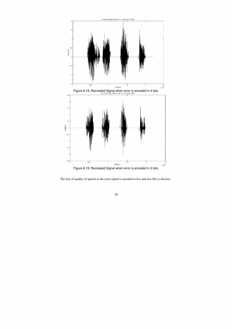
Figure 6.18: Recreated Signal when error is encoded in 4 bits.
Figure 6.19: Recreated Signal when error is encoded in 3 bits.
The loss of quality of speech as the error signal is encoded in less and less bits is obvious.

7/23/2019 Linear Prediction for Speech Encoding
http://slidepdf.com/reader/full/linear-prediction-for-speech-encoding 60/102
60
Figure 6.20: Recreated Signal Spectrum when error is encoded in 8 bits.
Figure 6.21: Recreated Signal Spectrum when error is encoded in 7 bits.

7/23/2019 Linear Prediction for Speech Encoding
http://slidepdf.com/reader/full/linear-prediction-for-speech-encoding 61/102
61
Figure 6.22: Recreated Signal Spectrum when error is encoded in 6 bits.
Figure 6.23: Recreated Signal Spectrum when error is encoded in 5 bits.

7/23/2019 Linear Prediction for Speech Encoding
http://slidepdf.com/reader/full/linear-prediction-for-speech-encoding 62/102
62
Figure 6.24: Recreated Signal Spectrum when error is encoded in 4 bits.
Figure 6.25: Recreated Signal Spectrum when error is encoded in 3 bits.

7/23/2019 Linear Prediction for Speech Encoding
http://slidepdf.com/reader/full/linear-prediction-for-speech-encoding 63/102
63
Chapter 7
Conclusions and Future Scope of the Project

7/23/2019 Linear Prediction for Speech Encoding
http://slidepdf.com/reader/full/linear-prediction-for-speech-encoding 64/102
64
7.1 Conclusions
From our experiments we have verified the accuracy and the efficiency of the Levinson
Durbin algorithm and its application to Linear Prediction. We have also clearly shown
that it is possible to compress speech signals in the form of forward prediction error
together with the filter parameters. If the error sample is stored in sufficient number of
bits then the recreated signal is of good quality.
As we have shown above we have managed to encode 8 bit speech sample into a 4 bit
error value while maintaining intelligibility of the speech. Depending on the application
and the quality of signal required we can choose the number of bits of precision to store
the error signal.
Our results show that use of windowing and segmentation is very useful in order to have
an efficient compression of the error signal.
The simulations results show that the prediction order in the range of 8-12 is sufficient
for linear prediction of speech, and using order above this does not give much
improvements.
Figures obtained by our simulations on MATLAB6.1 show that a window size of 5-10
msec gives very good results for speech samples at 11025 Hz. For good results, the
length of the window should contain ideally 60 to 100 speech samples.

7/23/2019 Linear Prediction for Speech Encoding
http://slidepdf.com/reader/full/linear-prediction-for-speech-encoding 65/102
65
7.2 Future Scope of the Project
In our project we successfully simulated compression of speech in MATLAB. We also
made all the relevant functions on our own so that all the work can be easily implemented
in Hardware.
Future students working on this project will find the hardware implementation of our
project very simple as we have provided a ready made set of important functions along
with the source code. These functions can be easily coded in C language from which it
can be converted into the assembly language of any hardware.
Future work on the project can also be done on improved DSP techniques to further
reduce error and make compression more efficient.
The Linear Predictor Coefficients can be calculated faster using Schur Algorithm on
parallel architecture, which is much more computationally efficient. Hence real-time
speech processing can be performed.

7/23/2019 Linear Prediction for Speech Encoding
http://slidepdf.com/reader/full/linear-prediction-for-speech-encoding 66/102
66
8. References
[1] J.Makhoul, Linear Prediction: A tutorial review; Proc of IEEE, vol 63, pp 561-589,
April 1975.
[2] John D Markel and A H Gray, A linear prediction vocoder simulation based upon the
autocorrelation method, IEEE Tran. on Acoustics, speech and signal processing; Vol.
ASSP: 22, April 1974.
[3] L.R Rabiner, B S Atal amd M R Sambur, LPC prediction arror: analysis of its
variation with position of analysis frame, IEEE Tran. on Acoustics, speech and signal
processing; Vol. ASSP: 25, Oct 1977.
[4] Advanced Digital Signal Processing, Proakis J.G, Rader M.C, Ling F, Nikias C.L,
Macmillan Publishing Company, New York, 1992. ISBN- 0-02-396841-9.
[5] J.Makhoul, Stable and efficient Lattice Methods for Linear Prediction., IEEE Tran.
On Acoustic Speech and Signal Processing, Vol. ASSP: 25, Oct 1977
[6] Douglas O’Shaughnessy, Linear Predictive Coding, IEEE Potentials, Feb-1988
[7] John E. Roberts and R. H. Wiggins, PIECEWISE LINEAR PREDICTIVE CODING
(PLPC), The MITRE Corporation, Bedford, Massachusetts 01730, May-1980
[8] M. A. Atashroo, Autocorrelation Prediction, Advanced Research Project Agency.
[9] Manfred R. Schroeder, Linear Predictive Coding of Speech: Review and Current
Directions, IEEE Communications Magazine, Aug-1985, Vol-23, No. 8, pp 54-61
[10] Advanced Digital Signal Processing and Noise Reduction, Vaseghi Saeed V, John
Wiley and Sons, 1996. ISBN-0-471-62692-9.
[11] L.R Rabiner and B.H Juang, Fundamentals of Speech Processing, Prentice Hall,
1993.
[12] Simon Haykin, Adaptive Filter Theory, 3rd
edition, Prentice Hall International, New-
Jersey, ISBN 0-13-397985-7

7/23/2019 Linear Prediction for Speech Encoding
http://slidepdf.com/reader/full/linear-prediction-for-speech-encoding 67/102
67
Appendices

7/23/2019 Linear Prediction for Speech Encoding
http://slidepdf.com/reader/full/linear-prediction-for-speech-encoding 68/102
68
A. Appendix I: New MATLAB Functions.
Function A.1: The Levinson-Durbin Algorithm.
function [lpc_coeffs, ref_coeffs]=levdurbin(samples,num_coeff)
%syntax => [lpc_coeffs, ref_coeffs]=levdurbin(auto_mat,num_coeff) function for
calculating the LPC and %reflection coeffs
%input needed are the autocorrelation matrix and number of coefficients .
%Made by Vidhu Niti Singh-565\ECE\99 and Sandeep Dabas-549\ECE\99.
%finding the autocorrelation matrix
N=length(samples);
p=num_coeff;
auto_corr=zeros(p,p);
for k=1:p
for j=1:p
for n=p+1:N
auto_corr(k,j)=auto_corr(k,j)+samples(n-k).*samples(n-j);
end
end
end
%Reading the Auto-correlation Matrix and extracting R_dash(0),R_dash(1) ..
for i=1:num_coeff
R(i)=auto_corr(1,i);
end
%%%%%%%%%%%%%%%%%%%%%%%%%%%%%%%%%%%%%%%%%%%
E=0; % initialising the error term.

7/23/2019 Linear Prediction for Speech Encoding
http://slidepdf.com/reader/full/linear-prediction-for-speech-encoding 69/102
69
k=zeros(1,num_coeff); %initialising the reflection coeff matrix
a=zeros(num_coeff); %initialising the coeff pXp with no overwriting the previous
entries
E=R(0+1); % in the form of aurocorrelation + 1 because matrix index has to
be from 1
if R(1)==0 % To prevent divide by zero.
R(1)=1;
end
k(1)=-R(1+1)./R(0+1);
a(1,1)=k(1);
for j=2:num_coeff
E=0;
temp1=0;
temp2=0;
for L=1:j-1
temp1=temp1+a(j-1,L).*R(j-L+1);
end
for m=1:j-1
temp2=temp2+R(j-m+1).*a(j-1,j-m);
E=R(0+1)+temp2;
end
k(j)=-(R(j-1+1)+temp1)./E;
a(j,j)=k(j);
for m=1:j-1
a(j,m)=a(j-1,m)+k(j).*a(j-1,j-m);
end
end
lpc_coeffs=[1 a(p,:)];
ref_coeffs=k;

7/23/2019 Linear Prediction for Speech Encoding
http://slidepdf.com/reader/full/linear-prediction-for-speech-encoding 70/102
70
Function A.2: Ntoone
function output=Ntoone(sample)
%output=Ntoone(sample)
%This is a function for converting an N dimension matrix to 1 dimension
%matrix
%The input parameter is an N dimensional matrix and the
%output is a one dimensional matrix
%Made by Vidhu Niti Singh-565\ECE\99 and Sandeep Dabas-549\ECE\99.
[R,C]=size(sample);
output=zeros(1,R*C);
for i=1:R
for j=1:C
output(1,(i-1)*C+j)=sample(i,j);
end
end

7/23/2019 Linear Prediction for Speech Encoding
http://slidepdf.com/reader/full/linear-prediction-for-speech-encoding 71/102
71
Function A.3: onetoN
function output=onetoN(sample,R,C)
%output=onetoN(sample,R,C)
%Function for converting a one dimensional matrix into a
%N dimension matrix.
%The input parameter is an one dimensional matrix and the number
%of rows and columns
%The output is a N dimensional matrix
%Made by Vidhu Niti Singh-565\ECE\99 and Sandeep Dabas-549\ECE\99.
len=length(sample);
output=zeros(R,C);
for i=1:R
for j=1:C
output(i,j)=sample((i-1)*C+j);
end
end

7/23/2019 Linear Prediction for Speech Encoding
http://slidepdf.com/reader/full/linear-prediction-for-speech-encoding 72/102
72
Function A.4: onetoN
function
one_D=Ntoone_overlap(windowed_samples,padded_number_of_windows,padded_
window_length)
%Syntax=>one_D=Ntoone_overlap(windowed_samples,padded_number_of_windows,p
added_window_le%ngth)
%The input parameters are as follows
%windowed samples = matrix returned after windowing, which contains overlapping
elements.
%padded_number of windows = Number of windows after equalizing the size of the
sample and the
%lenght required for windowing.
%padded_window_length = Length after equalizing all sizes
%This function is used in conjunction with the overlapping windowing
%function and converts a N dimensional matrix having overlapping windows to a one
%dimensional matrix in such a way that the overlapping elements are considered only
once
%and not twice.
%Made by Vidhu Niti Singh-565\ECE\99 and Sandeep Dabas-549\ECE\99.
one_D=zeros(1,padded_number_of_windows*(padded_window_length/2)+padded_wind
ow_length/2);
for i=0:padded_number_of_windows-1
for j=1:padded_window_length

7/23/2019 Linear Prediction for Speech Encoding
http://slidepdf.com/reader/full/linear-prediction-for-speech-encoding 73/102
73
one_D(1,(i*(padded_window_length/2)+j))=one_D(1,(i*(padded_window_length/2)+j))
+ windowed_samples(i+1,j);
end
end

7/23/2019 Linear Prediction for Speech Encoding
http://slidepdf.com/reader/full/linear-prediction-for-speech-encoding 74/102
74
Function A.5: rect_win
function [windowed_samples, padded_window_length,
padded_number_of_windows]=rect_win(samples,sam_rate,time_segment)
%syntax =>[windowed_samples, padded_window_length,
%padded_number_of_windows]=rect_win(samples,sam_rate,time_segment)
%The function is used for the purpose of segmentation and windowing a speech sample.
The segments
%are non overlapping and the window type is rectangular. Non-overlapping segments
use each value
%onle once for the purpose of windowing.
%samples = The matrix containing the signal to be segmented and windowed.
%sam_rate = The sampling rate of the speech signal
%time segment = The length of the window in milli seconds i.e. length of the time
segment
%Made by Vidhu Niti Singh-565\ECE\99 and Sandeep Dabas-549\ECE\99.
win_length=sam_rate*time_segment;
padded_window_length=ceil(win_length);
number_of_windows=length(samples)/win_length;
padded_number_of_windows=ceil(number_of_windows);
padded_total_length=padded_number_of_windows * padded_window_length;
padded_samples=[samples' zeros(1,padded_total_length-length(samples))];
windowed_samples=zeros(padded_number_of_windows,padded_window_length);
for i=0:padded_number_of_windows-1
for j=1:padded_window_length
windowed_samples(i+1,j)=padded_samples(i*padded_window_length+j);
end
end

7/23/2019 Linear Prediction for Speech Encoding
http://slidepdf.com/reader/full/linear-prediction-for-speech-encoding 75/102
75
Function A.6: han_win_overlap
function [windowed_samples, padded_window_length,
padded_number_of_windows]=ham_win_overlap(samples,sam_rate,time_segment)
%syntax =>[windowed_samples, padded_window_length,
%padded_number_of_windows]=ham_win_overlap(samples,sam_rate,time_segment)
%This function is used for segmenation and windowing of input speech signal.
%The segmenation type is overlapping with an i=overlap of N/2 where N is the window
size.
%The windowing type is hamming window.
%This function can be used for other types of windowing such as hanning rectangular
%by changing the multiplying value.
%The input parameters are
%samples = The matrix containing the signal to be segmented and windowed.
%sam_rate = The sampling rate of the speech signal
%time segment = The length of the window in milli seconds i.e. length of the time
segment
%Made by Vidhu Niti Singh-565\ECE\99 and Sandeep Dabas-549\ECE\99.
win_length=sam_rate*time_segment;
padded_window_length=ceil(win_length);
if rem(padded_window_length,2)==1
padded_window_length=padded_window_length+1;
end
i=0;
while (length(samples)-i*(padded_window_length./2))>padded_window_length
for j=1:padded_window_length

7/23/2019 Linear Prediction for Speech Encoding
http://slidepdf.com/reader/full/linear-prediction-for-speech-encoding 76/102
76
windowed_samples(i+1,j)=samples(1,i*(padded_window_length/2)+j).*(0.50-
0.50.*(cos((2*pi*(j-1)./(padded_window_length-1)))));
end
i=i+1;
end
for j=1:padded_window_length
if i*(padded_window_length/2)+j < length(samples)
windowed_samples(i+1,j)=samples(1,i*(padded_window_length/2)+j).*(0.50-
0.50.*(cos((2*pi*(j-1)./(padded_window_length-1)))));
else
windowed_samples(i+1,j)=0;
end
end
padded_number_of_windows=i+1;

7/23/2019 Linear Prediction for Speech Encoding
http://slidepdf.com/reader/full/linear-prediction-for-speech-encoding 77/102
77
Function A.7: fir_cpp
function [y]=fir_cpp(b,a,x)
% syntax =>[y]=fir_cpp(b,a,x)
% This function is a self made function for implementation of an FIR filter
% The inputs are the standard inputs which are given to the MATLAB filter command.
%Made by Vidhu Niti Singh-565\ECE\99 and Sandeep Dabas-549\ECE\99.
p=length(b);
p=p-1;
temp=zeros(p+1,1);
N=length(x);
for i=1:N
for j=1:p+1
if i-j >=0
temp(j,1)=x(i-j+1);
end
end
b_tran=b;
y(i)=b_tran*temp;
end

7/23/2019 Linear Prediction for Speech Encoding
http://slidepdf.com/reader/full/linear-prediction-for-speech-encoding 78/102
78
Function A.8: iir_cpp
function [y]=iir_cpp(b,a,x)
% syntax =>[y]=fir_cpp(b,a,x)
% This function is a self made function for implementation of an IIR filter
% The inputs are the standard inputs which are given to the MATLAB filter command.
%Made by Vidhu Niti Singh-565\ECE\99 and Sandeep Dabas-549\ECE\99.
p=length(a);
for k=2:p
q(1,k-1)=a(k);
end
p=p-1;
temp=zeros(p,1);
N=length(x);
y=zeros(1,N);
for i=1:N
for j=1:p
if i-j >0
temp(j,1)=y(i-j);
end
end
%q_tran=q';
y(i)=q*temp;
y(i)=-y(i)+x(i);
end

7/23/2019 Linear Prediction for Speech Encoding
http://slidepdf.com/reader/full/linear-prediction-for-speech-encoding 79/102
79
Function A.9: lat_cpp
function [output] = lat_cpp(b,x)
%syntax =>[output] = lat_cpp(b,x)
%This function is for a all zero lattice filter. This filter is equivalent to an iir filter.
%The inputs required are the reflection coefficients and the input to be sampled
%Made by Vidhu Niti Singh-565\ECE\99 and Sandeep Dabas-549\ECE\99.
N=length(x);
p=length(b);
F=zeros(p+1,N);
G=zeros(p+1,N);
F(1,:)=x;
G(1,:)=x;
for j=2:N
for i=2:p+1
F(i,j) = F(i-1,j) + b(i-1)*G(i-1,j-1); % here we r generating the output of
lattice filter i.e error
G(i,j) = b(i-1)*F(i-1,j) + G(i-1,j-1);
end
end
output=F(p+1,:);
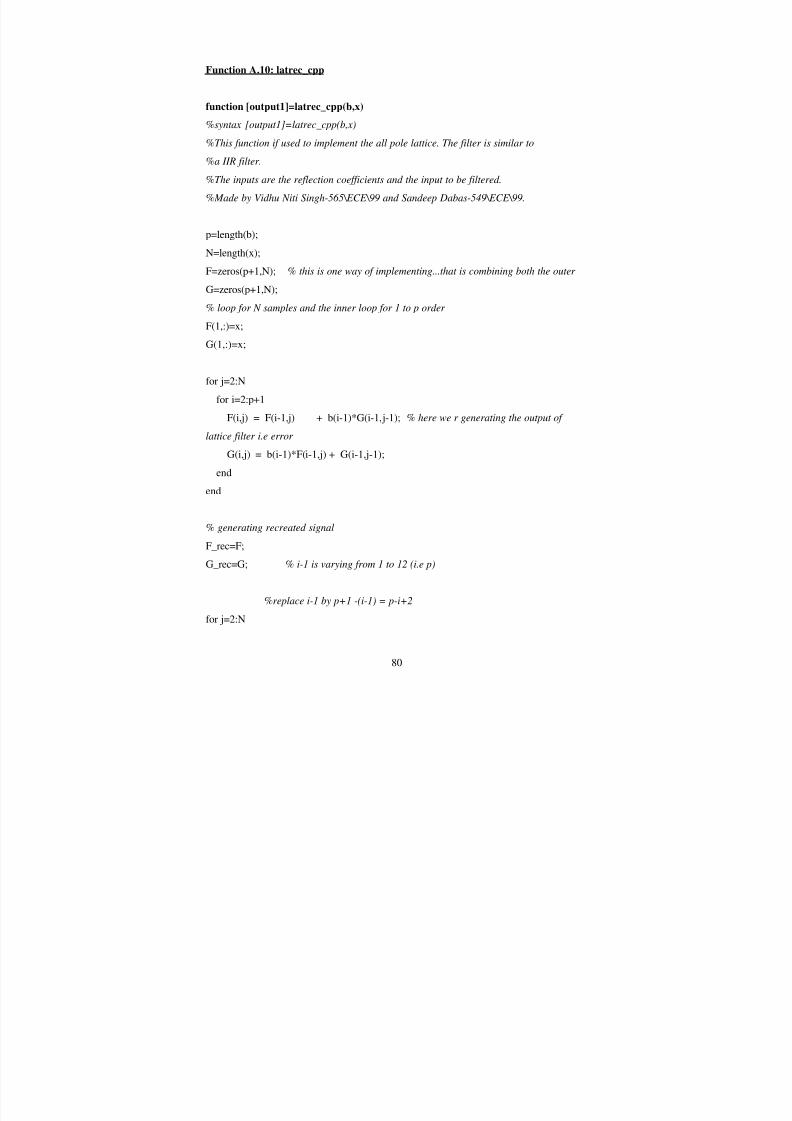
7/23/2019 Linear Prediction for Speech Encoding
http://slidepdf.com/reader/full/linear-prediction-for-speech-encoding 80/102
80
Function A.10: latrec_cpp
function [output1]=latrec_cpp(b,x)
%syntax [output1]=latrec_cpp(b,x)
%This function if used to implement the all pole lattice. The filter is similar to
%a IIR filter.
%The inputs are the reflection coefficients and the input to be filtered.
%Made by Vidhu Niti Singh-565\ECE\99 and Sandeep Dabas-549\ECE\99.
p=length(b);
N=length(x);
F=zeros(p+1,N); % this is one way of implementing...that is combining both the outer
G=zeros(p+1,N);
% loop for N samples and the inner loop for 1 to p order
F(1,:)=x;
G(1,:)=x;
for j=2:N
for i=2:p+1
F(i,j) = F(i-1,j) + b(i-1)*G(i-1,j-1); % here we r generating the output of
lattice filter i.e error
G(i,j) = b(i-1)*F(i-1,j) + G(i-1,j-1);
end
end
% generating recreated signal
F_rec=F;
G_rec=G; % i-1 is varying from 1 to 12 (i.e p)
%replace i-1 by p+1 -(i-1) = p-i+2
for j=2:N

7/23/2019 Linear Prediction for Speech Encoding
http://slidepdf.com/reader/full/linear-prediction-for-speech-encoding 81/102
81
for i=2:p+1 % here we r getting back the recreated signal
F_rec(p-i+2,j) = F_rec(p-i+3,j) - b(p-i+2)*G_rec(p-i+2,j-1);
G_rec(p-i+3,j) = b(p-i+2)*F_rec(p-i+2,j) + G_rec(p-i+2,j-1);
end
end
output1=F_rec(1,:);

7/23/2019 Linear Prediction for Speech Encoding
http://slidepdf.com/reader/full/linear-prediction-for-speech-encoding 82/102
82
Function A.11: threshold
function out=threshhold(in,min)
%syntax =>out=threshhold(in,min)
% This function is used for end detection. The imputs are the input speech signal and the
% threshhold value below which the signal should be rejected.
%Made by Vidhu Niti Singh-565\ECE\99 and Sandeep Dabas-549\ECE\99.
N=length(in)
j=1;
max=30;
for i=1:N-max
if abs(in(i))>min
out(j)=in(i);
j=j+1;
else
for k=1:max
if abs(in(i+k))>min
out(j)=in(i);
j=j+1;
break
end
end
end
end
out=out-mean(out);

7/23/2019 Linear Prediction for Speech Encoding
http://slidepdf.com/reader/full/linear-prediction-for-speech-encoding 83/102
83
B. Appendix II: MATLAB Codes
Code B.1: Calculation of the Error Signal and Recreation of Speech.
% In this program we use the filter approach to find the error signal and then recreate
%the sample
% from the error. This is same as assuming a causal and causally invertible filter which
%converts
% a white noise sequence into a WSS process and the inverse filter which gives white
%noise output
% when a WSS process is taken as the input.
samples=readwav('vid2.wav');
p=12; % number of coefficients ie order of the predictor
N=length(samples);
y=levdurbin(samples,p);%<----using my own function.
%------------- making a predictive filter which gives error as the output ---------------
% the error can be treated as a white noise which is made after removing all the
%correlation
% in the input speech sample.
b=y;
a=1;
error=filter(b,a,samples);
%----------Passing the error through the inverse filter which again generates the speech
%sample.
a_dash=y;

7/23/2019 Linear Prediction for Speech Encoding
http://slidepdf.com/reader/full/linear-prediction-for-speech-encoding 84/102
84
b_dash=1;
recreate=filter(b_dash,a_dash,error);
subplot(3,1,1),plot(samples);title('Original Signal');axis([0 length(samples) –1 1]);
xlabel('Samples');ylabel('Amplitude');
subplot(3,1,2),plot(error);title('Error Signal');axis([0 length(samples) -1 1 ] ) ;
xlabel('Samples');ylabel('Amplitude');
subplot(3,1,3),plot(recreate);title('Recreated Signal');axis([0 length(samples) -1 1 ] ) ;
xlabel('Samples');ylabel('Amplitude');

7/23/2019 Linear Prediction for Speech Encoding
http://slidepdf.com/reader/full/linear-prediction-for-speech-encoding 85/102
85
Code B.2: Non-Overlapping Segmentation of Speech Sample
%This program segments the sample by using windowing. We want to see the effect on
%the forward %prediction error by using this technique. The forward prediction error
%should decrease.
[samples sam_rate FIDX Wmode]=readwav('vid2.wav');
samples=threshhold(samples,0.03);[windowed_samples padded_window_length padded_number_of_windows]
=rect_win(samples' ,sam_rate,0.015);
p=8; %order of prediction
lpc_matrix=zeros(padded_number_of_windows,1+p);
error=zeros(padded_number_of_windows,padded_window_length);
for i=0:padded_number_of_windows-1lpc_matrix(i+1,:)=levdurbin(windowed_samples(i+1,:),p);error(i+1,:)=fir_cpp(lpc_matrix(i+1,:),1,windowed_samples(i+1 ,:)); %passing
through noise %whitening filter
end
recreated=zeros(padded_number_of_windows,padded_window_length);
for i=0:padded_number_of_windows-1
for j=1:padded_window_length
recreated(i+1,:)=iir_cpp(1,lpc_matrix(i+1,:),error(i+1,:)); %passing through inverse
filter
end
end
error_1d=zeros(1,padded_number_of_windows*padded_window_length);
recreated_1d=zeros(1,padded_number_of_windows*padded_window_length);
error_1d=reshape(error',1,padded_number_of_windows*padded_window_length);
recreated_1d=reshape(recreated',1,padded_number_of_windows*padded_window_length
);
subplot(3,1,1);plot(samples);title('Original signal');axis([0 length(samples) -1 1]);
ylabel('Amplitude'); subplot(3,1,2);plot(error_1d);title('Error signal(windowed)');axis([0 length(samples) -1 1]); ylabel('Amplitude');
subplot(3,1,3);plot(recreated_1d);title('Recreated signal');
axis([0 length(samples) -1 1]);ylabel('Amplitude');

7/23/2019 Linear Prediction for Speech Encoding
http://slidepdf.com/reader/full/linear-prediction-for-speech-encoding 86/102
86
Code B.3: Calculation of the Error Signal and Recreation of Speech.
%In this program the Speech Segment is segmented into overlapping segments and
%Hanning Window is %used on each segment.
%The size of each segment is 15 millisecond.
[samples sam_rate FIDX Wmode]=readwav('vid2');
samples=threshhold(samples,0.030);
[windowed_samples padded_window_length
padded_number_of_windows]=han_win_overlap(samples,sam_rate,0.015);
p=8;% number of coefficients ie order of the predictor
lpc_matrix=zeros(padded_number_of_windows,1+p);
error=zeros(padded_number_of_windows,padded_window_length);
for i=0:padded_number_of_windows-1
lpc_matrix(i+1,:)=levdurbin(windowed_samples(i+1,:),p);
error(i+1,:)=fir_cpp(lpc_matrix(i+1,:),1,windowed_samples(i+1,:));
end
figure(1);
one_D=Ntoone_overlap(error,padded_number_of_windows,padded_window_length);
recreated=zeros(padded_number_of_windows,padded_window_length);
for i=0:padded_number_of_windows-1
recreated(i+1,:)=iir_cpp(1,lpc_matrix(i+1,:),error(i+1,:));
end
recreated_1d=Ntoone_overlap(recreated,padded_number_of_windows,padded_window_l
ength);
subplot(3,1,2);plot(one_D);title('overlap window error');axis([0 length(samples) -.6 .6]);

7/23/2019 Linear Prediction for Speech Encoding
http://slidepdf.com/reader/full/linear-prediction-for-speech-encoding 87/102
87
subplot(3,1,1);plot(samples);title('Original Signal');axis([0 length(samples) -.6 .6]);
subplot(3,1,3);plot(recreated_1d);title('Recreated Signal');axis([0 length(samples) -.6 .6]);

7/23/2019 Linear Prediction for Speech Encoding
http://slidepdf.com/reader/full/linear-prediction-for-speech-encoding 88/102
88
Code B.4: Encoding of error signal using different number of bits
%In this program we encode the error signal into different number of bits and %then
%read it back to
%take the effect of quantisation into effect.
%-------------Reading the file ------------------------
[samples,sam_rate,wmode,fidx]=readwav('vid2.wav');
p=8; % number of coefficients ie order of the predictor
N=length(samples);
[windowed_samples padded_window_length
padded_number_of_windows]=han_win_overlap(samples',sam_rate,0.015);
lpc_matrix=zeros(padded_number_of_windows,1+p);
error=zeros(padded_number_of_windows,padded_window_length);
for i=0:padded_number_of_windows-1
lpc_matrix(i+1,:)=real(lpc(windowed_samples(i+1,:),p));
error(i+1,:)=fir_cpp(lpc_matrix(i+1,:),1,windowed_samples(i+1,:));
end
one_D=Ntoone_overlap(error,padded_number_of_windows,padded_window_length);
writewav(one_D,sam_rate,'error_8.wav','8','s');
writewav(one_D,sam_rate,'error_7.wav','7','s');
writewav(one_D,sam_rate,'error_6.wav','6','s');
writewav(one_D,sam_rate,'error_5.wav','5','s');
writewav(one_D,sam_rate,'error_4.wav','4','s');
writewav(one_D,sam_rate,'error_3.wav','3','s');

7/23/2019 Linear Prediction for Speech Encoding
http://slidepdf.com/reader/full/linear-prediction-for-speech-encoding 89/102
89
error_8=readwav('error_8','s');
error_7=readwav('error_7','s');
error_6=readwav('error_6','s');
error_5=readwav('error_5','s');
error_4=readwav('error_4','s');
error_3=readwav('error_3','s');
err=error_8;
error=onetoN_overlap(err',padded_number_of_windows,padded_window_length);
recreated=zeros(padded_number_of_windows,padded_window_length);
for i=0:padded_number_of_windows-1
recreated(i+1,:)=iir_cpp(1,lpc_matrix(i+1,:),error(i+1,:));
end
recreated_1d=Ntoone_overlap(recreated,padded_number_of_windows,padded_window_l
ength);
writewav(recreated_1d,sam_rate,'recreated_8');
subplot(3,1,1);plot(samples);title('original signal');axis([0 length(samples) -.6
.6]);ylabel('Amplitute');
subplot(3,1,2);plot(one_D);title('error signal');axis([0 length(samples) -.6
.6]);ylabel('Amplitute');
subplot(3,1,3);plot(recreated_1d);title('Recreated Signal');
axis([0 length(samples) -2.5 2.5]);ylabel('Amplitute');

7/23/2019 Linear Prediction for Speech Encoding
http://slidepdf.com/reader/full/linear-prediction-for-speech-encoding 90/102
90
C. Appendix III C- Codes
Code C.1 Levinson Durbin Algorithm
#include "levd.h"
M levd(M samples, M num_coeff) {
double old_nargin=nargin; nargin=2; nargin_set=1;
double old_nargout=nargout; nargout=1; nargout_set=1;
M lpc_coeffs__out(0,0,"lpc_coeffs__out");
levd(samples, num_coeff, i_o, lpc_coeffs__out, junk_M);
nargout=old_nargout;
nargin=old_nargin;
return(lpc_coeffs__out);
}
M levd(M samples, M num_coeff, i_o_t, Mr lpc_coeffs__out, Mr ref_coeffs__out) {
M ans(0,0,"ans"), lpc_coeffs(0,0,"lpc_coeffs"), ref_coeffs(0,0,"ref_coeffs")\
, N(0,0,"N"), p(0,0,"p"), auto_corr(0,0,"auto_corr"), k(0,0,"k"), k_v0(\
0,0,"k_v0"), j(0,0,"j"), j_v1(0,0,"j_v1"), n(0,0,"n"), n_v2(0,0,"n_v2")\
, i(0,0,"i"), i_v3(0,0,"i_v3"), R(0,0,"R"), E(0,0,"E"), a(0,0,"a"), j_v4(\
0,0,"j_v4"), temp1(0,0,"temp1"), temp2(0,0,"temp2"), L(0,0,"L"), L_v5(0,\
0,"L_v5"), m(0,0,"m"), m_v6(0,0,"m_v6"), m_v7(0,0,"m_v7");
double old_nargin=nargin; if (!nargin_set) nargin =2;
double old_nargout=nargout; if (!nargout_set) nargout=2;
nargin_set=0; nargout_set=0;
N=length(samples);
p=num_coeff;
auto_corr=zeros(p,p);

7/23/2019 Linear Prediction for Speech Encoding
http://slidepdf.com/reader/full/linear-prediction-for-speech-encoding 91/102
91
k_v0=colon(1.0,1,p);
for (int k_i0=1;k_i0<=forsize(k_v0);k_i0++) {
forelem(k,k_v0,k_i0);
j_v1=colon(1.0,1,p);
for (int j_i1=1;j_i1<=forsize(j_v1);j_i1++) {
forelem(j,j_v1,j_i1);
n_v2=colon(p+1.0,1,N);
for (int n_i2=1;n_i2<=forsize(n_v2);n_i2++) {
forelem(n,n_v2,n_i2);
auto_corr(k,j)=auto_corr(k,j)+dot_mul(samples(n-k),samples(n-j)\
);
}
}
}
//Reading the Auto-correlation Matrix and extracting R_dash(0),R_dash(1) ..
i_v3=colon(1.0,1,num_coeff);
for (int i_i3=1;i_i3<=forsize(i_v3);i_i3++) {
forelem(i,i_v3,i_i3);
R(i)=auto_corr(1.0,i);
}
//%%%%%%%%%%%%%%%%%%%%%%%%%%%%%%%%%%%%%%%%%%
E=0.0;
// initialising the error term.
k=zeros(1.0,num_coeff);
//initialising the reflection coeff matrix
a=zeros(num_coeff);
//initialising the coeff pXp with no overwriting the previous entries
E=R(0.0+1.0);
//% in the form of aurocorrelation + 1 because matrix index has to be from 1
if (istrue(R(1.0)==0.0)) {

7/23/2019 Linear Prediction for Speech Encoding
http://slidepdf.com/reader/full/linear-prediction-for-speech-encoding 92/102
92
// To prevent divide by zero.
R(1.0)=1.0;
}
k(1.0)=-dot_div(R(1.0+1.0),R(0.0+1.0));
a(1.0,1.0)=k(1.0);
j_v4=colon(2.0,1,num_coeff);
for (int j_i4=1;j_i4<=forsize(j_v4);j_i4++) {
forelem(j,j_v4,j_i4);
E=0.0;
temp1=0.0;
temp2=0.0;
L_v5=colon(1.0,1,j-1.0);
for (int L_i5=1;L_i5<=forsize(L_v5);L_i5++) {
forelem(L,L_v5,L_i5);
temp1+=dot_mul(a(j-1.0,L),R(j-L+1.0));
}
m_v6=colon(1.0,1,j-1.0);
for (int m_i6=1;m_i6<=forsize(m_v6);m_i6++) {
forelem(m,m_v6,m_i6);
temp2+=dot_mul(R(j-m+1.0),a(j-1.0,j-m));
E=R(0.0+1.0)+temp2;
}
k(j)=-dot_div((R(j-1.0+1.0)+temp1),E);
a(j,j)=k(j);
m_v7=colon(1.0,1,j-1.0);
for (int m_i7=1;m_i7<=forsize(m_v7);m_i7++) {
forelem(m,m_v7,m_i7);
a(j,m)=a(j-1.0,m)+dot_mul(k(j),a(j-1.0,j-m));
}
}
lpc_coeffs=brackets('M',(M)1.0,(M)a(p,c_p),l_M);

7/23/2019 Linear Prediction for Speech Encoding
http://slidepdf.com/reader/full/linear-prediction-for-speech-encoding 93/102
93
ref_coeffs=k;
nargin=old_nargin; nargout=old_nargout;
lpc_coeffs__out=lpc_coeffs; ref_coeffs__out=ref_coeffs; return(nop_M)\
;
}
main() {
initM();
levd();
exitM();
return 0;
}
Code C.2 Levinson Durbin Header File
#ifndef __levd_h
#define __levd_h
#include "matlib.h"
M levd(M samples, M num_coeff);
M levd(M samples, M num_coeff, i_o_t, Mr lpc_coeffs__out, Mr ref_coeffs__out);
#endif

7/23/2019 Linear Prediction for Speech Encoding
http://slidepdf.com/reader/full/linear-prediction-for-speech-encoding 94/102
94
Code C.3 MA Lattice Filter
#include "lat.h"
M lat(M b, M x) {
M ans(0,0,"ans"), output(0,0,"output"), N(0,0,"N"), p(0,0,"p"), F(0,0,"F")\
, G(0,0,"G"), j(0,0,"j"), j_v0(0,0,"j_v0"), i(0,0,"i"), i_v1(0,0,"i_v1")\
;
double old_nargin=nargin; if (!nargin_set) nargin =2;
double old_nargout=nargout; if (!nargout_set) nargout=1;
nargin_set=0; nargout_set=0;
//syntax =>[output] = lat_cpp(b,x)
N=length(x);
p=length(b);
F=zeros(p+1.0,N);
G=zeros(p+1.0,N);
F(1.0,c_p)=x;
G(1.0,c_p)=x;
j_v0=colon(2.0,1,N);
for (int j_i0=1;j_i0<=forsize(j_v0);j_i0++) {
forelem(j,j_v0,j_i0);
i_v1=colon(2.0,1,p+1.0);
for (int i_i1=1;i_i1<=forsize(i_v1);i_i1++) {
forelem(i,i_v1,i_i1);
F(i,j)=F(i-1.0,j)+b(i-1.0)*G(i-1.0,j-1.0);
// here we r generating the output of lattice filter i.e error
G(i,j)=b(i-1.0)*F(i-1.0,j)+G(i-1.0,j-1.0);
}
}
output=F(p+1.0,c_p);

7/23/2019 Linear Prediction for Speech Encoding
http://slidepdf.com/reader/full/linear-prediction-for-speech-encoding 95/102
95
nargin=old_nargin; nargout=old_nargout;
return(output);
}
main() {
initM();
lat();
exitM();
return 0;
}
Code x.3 MA Lattice Filter Header File
#ifndef __lat_h
#define __lat_h
#include "matlib.h"
M lat(M b, M x);
#endif

7/23/2019 Linear Prediction for Speech Encoding
http://slidepdf.com/reader/full/linear-prediction-for-speech-encoding 96/102
96
Code C.3 AR Lattice Filter
#include "latrec.h"
M latrec(M b, M x) {
M ans(0,0,"ans"), output1(0,0,"output1"), p(0,0,"p"), N(0,0,"N"), F(0,0,\
"F"), G(0,0,"G"), j(0,0,"j"), j_v0(0,0,"j_v0"), i(0,0,"i"), i_v1(0,0,"i_v1")\
, F_rec(0,0,"F_rec"), G_rec(0,0,"G_rec"), j_v2(0,0,"j_v2"), i_v3(0,0,"i_v3")\
;
double old_nargin=nargin; if (!nargin_set) nargin =2;
double old_nargout=nargout; if (!nargout_set) nargout=1;
nargin_set=0; nargout_set=0;
p=length(b);
N=length(x);
F=zeros(p+1.0,N);
// this is one way of implementing...that is combining both the outer
G=zeros(p+1.0,N);
// loop for N samples and the inner loop for 1 to p order
F(1.0,c_p)=x;
G(1.0,c_p)=x;
j_v0=colon(2.0,1,N);
for (int j_i0=1;j_i0<=forsize(j_v0);j_i0++) {
forelem(j,j_v0,j_i0);
i_v1=colon(2.0,1,p+1.0);
for (int i_i1=1;i_i1<=forsize(i_v1);i_i1++) {forelem(i,i_v1,i_i1);
F(i,j)=F(i-1.0,j)+b(i-1.0)*G(i-1.0,j-1.0);
// here we r generating the output of lattice filter i.e error
G(i,j)=b(i-1.0)*F(i-1.0,j)+G(i-1.0,j-1.0);
}

7/23/2019 Linear Prediction for Speech Encoding
http://slidepdf.com/reader/full/linear-prediction-for-speech-encoding 97/102
97
}
// generating recreated signal
F_rec=F;
G_rec=G;
// i-1 is varying from 1 to 12 (i.e p)
//replace i-1 by p+1 -(i-1) = p-i+2
j_v2=colon(2.0,1,N);
for (int j_i2=1;j_i2<=forsize(j_v2);j_i2++) {
forelem(j,j_v2,j_i2);
i_v3=colon(2.0,1,p+1.0);
for (int i_i3=1;i_i3<=forsize(i_v3);i_i3++) {
forelem(i,i_v3,i_i3);
// here we r getting back the recreated signal
F_rec(p-i+2.0,j)=F_rec(p-i+3.0,j)-b(p-i+2.0)*G_rec(p-i+2.0,j-1.0)\
;
G_rec(p-i+3.0,j)=b(p-i+2.0)*F_rec(p-i+2.0,j)+G_rec(p-i+2.0,j-1.0)\
;
}
}
output1=F_rec(1.0,c_p);
nargin=old_nargin; nargout=old_nargout;
return(output1);
}
main() {
initM();
latrec();
exitM();
return 0;
}

7/23/2019 Linear Prediction for Speech Encoding
http://slidepdf.com/reader/full/linear-prediction-for-speech-encoding 98/102
98
Code C.3 AR Lattice Filter Header File
#ifndef __latrec_h
#define __latrec_h
#include "matlib.h"
M latrec(M b, M x);
#endif

7/23/2019 Linear Prediction for Speech Encoding
http://slidepdf.com/reader/full/linear-prediction-for-speech-encoding 99/102
99
Code C.3 Segmentation and Hanning Window
#include "hanwin.h"
M hanwin(M samples, M sam_rate, M time_segment) {
double old_nargin=nargin; nargin=3; nargin_set=1;
double old_nargout=nargout; nargout=1; nargout_set=1;
M windowed_samples__out(0,0,"windowed_samples__out");
hanwin(samples, sam_rate, time_segment, i_o, windowed_samples__out, junk_M,
junk_M);
nargout=old_nargout;nargin=old_nargin;
return(windowed_samples__out);
}
M hanwin(M samples, M sam_rate, M time_segment, i_o_t, Mr
windowed_samples__out, Mr padded_window_length__out) {
double old_nargin=nargin; nargin=3; nargin_set=1;
double old_nargout=nargout; nargout=2; nargout_set=1;
hanwin(samples, sam_rate, time_segment, i_o, windowed_samples__out,
padded_window_length__out, junk_M);
nargout=old_nargout;
nargin=old_nargin;
return(sixpack_M);
}
M hanwin(M samples, M sam_rate, M time_segment, i_o_t, Mr
windowed_samples__out, Mr padded_window_length__out, Mr
padded_number_of_windows__out) {

7/23/2019 Linear Prediction for Speech Encoding
http://slidepdf.com/reader/full/linear-prediction-for-speech-encoding 100/102
100
M ans(0,0,"ans"), windowed_samples(0,0,"windowed_samples"),
padded_window_length(\
0,0,"padded_window_length"),
padded_number_of_windows(0,0,"padded_number_of_windows")\
, win_length(0,0,"win_length"), i(0,0,"i"), j(0,0,"j"), j_v0(0,0,"j_v0")\
, j_v1(0,0,"j_v1");
double old_nargin=nargin; if (!nargin_set) nargin =3;
double old_nargout=nargout; if (!nargout_set) nargout=3;
nargin_set=0; nargout_set=0;
win_length=sam_rate*time_segment;
padded_window_length=ceil(win_length);
if (istrue(rem(padded_window_length,2.0)==1.0)) {
padded_window_length+=1.0;
}
i=0.0;
while (istrue((length(samples)-i*(dot_div(padded_window_length,2.0)))\
>padded_window_length)) {
j_v0=colon(1.0,1,padded_window_length);
for (int j_i0=1;j_i0<=forsize(j_v0);j_i0++) {
forelem(j,j_v0,j_i0);
windowed_samples(i+1.0,j)=dot_mul(samples(1.0,i*(padded_window_length/2.0)\
+j),(0.5-dot_mul(0.5,(cos((dot_div(2.0*pi*(j-1.0),(padded_window_length-1.0)\
)))))));
}
i+=1.0;
}
j_v1=colon(1.0,1,padded_window_length);
for (int j_i1=1;j_i1<=forsize(j_v1);j_i1++) {
forelem(j,j_v1,j_i1);
if (istrue(i*(padded_window_length/2.0)+j<length(samples))) {
windowed_samples(i+1.0,j)=dot_mul(samples(1.0,i*(padded_window_length/2.0)\

7/23/2019 Linear Prediction for Speech Encoding
http://slidepdf.com/reader/full/linear-prediction-for-speech-encoding 101/102
101
+j),(0.5-dot_mul(0.5,(cos((dot_div(2.0*pi*(j-1.0),(padded_window_length-1.0)\
)))))));
} else {
windowed_samples(i+1.0,j)=0.0;
}
}
padded_number_of_windows=i+1.0;
nargin=old_nargin; nargout=old_nargout;
windowed_samples__out=windowed_samples;
padded_window_length__out=padded_window_length; \
padded_number_of_windows__out=padded_number_of_windows; return(nop_M)\
;
}
main() {
initM();
hanwin();
exitM();
return 0;
}
Code C.3 Segmentation and Hanning Window Header File
#ifndef __hanwin_h
#define __hanwin_h
#include "matlib.h"
M hanwin(M samples, M sam_rate, M time_segment);

7/23/2019 Linear Prediction for Speech Encoding
http://slidepdf.com/reader/full/linear-prediction-for-speech-encoding 102/102
M hanwin(M samples, M sam_rate, M time_segment, i_o_t, Mr
windowed_samples__out, Mr padded_window_length__out);
M hanwin(M samples, M sam_rate, M time_segment, i_o_t, Mr
windowed_samples__out, Mr padded_window_length__out, Mr
padded_number_of_windows__out);
#endif