LINEAR OPERATORS AND THE DISTRIBUTION

OF ZEROS OF ENTIRE FUNCTIONS

A DISSERTATION SUBMITTED TO THE GRADUATE DIVISION OF THEUNIVERSITY OF HAWAI‘I IN PARTIAL FULFILLMENT OF THE

REQUIREMENTS FOR THE DEGREE OF

DOCTOR OF PHILOSOPHY

IN

MATHEMATICS

MAY 2007

ByAndrzej Piotrowski

Dissertation Committee:

George L. Csordas, ChairpersonDavid BleeckerThomas CravenThomas HooverRobert D. Little

Benjamin K. Bergen

We certify that we have read this dissertation and that, in our opinion, it is

satisfactory in scope and quality as a dissertation for the degree of

Doctor of Philosophy in Mathematics.

DISSERTATION COMMITTEE

——————————————Chairperson

——————————————

——————————————

——————————————

——————————————

——————————————

ii

Acknowledgments

First and foremost, I would like to express my deep gratitude to Dr. George

Csordas for his constant enthusiasm, guidance, and support. I would also like to

thank my parents, Ted and Terri, my sisters, Ala and Renia, and also my close

friends, both in New Hampshire and Hawai‘i, for their encouragement. Finally, I

am grateful for the inspiration I have received from the students, faculty, and staff

of the mathematics departments at the two universities I have had the privilege of

attending: the University of New Hampshire and the University of Hawai‘i.

iii

Abstract

If {γk}∞k=0 is a sequence of real numbers and Q = {qk(x)}∞k=0 is a sequence of poly-

nomials satisfying deg(qk) = k for all non-negative integers k, then we can define a

linear operator TQ on the vector space of real polynomials by

TQ[qk(x)] = γkqk(x) (k = 0, 1, 2, . . . ).

If the linear operator TQ has the property that it maps every real polynomial having

only real zeros into another polynomial having only real zeros (or, perhaps, to the

identically zero function), then the corresponding sequence {γk}∞k=0 is called a Q-

multiplier sequence. Similarly, if the linear operator TQ has the property that it does

not increase the number of non-real zeros of any polynomial (which it does not map

to the identically zero function), then the corresponding sequence {γk}∞k=0 is called a

Q-complex zero decreasing sequence, or, for brevity, a Q-CZDS.

Polya and Schur completely characterized all multiplier sequences for the stan-

dard basis{xk}∞

k=0, which we will call the classical multiplier sequences. Turan,

and subsequently Bleecker and Csordas, discovered classes of H-multiplier sequences,

where H denotes the set of Hermite polynomials. In this dissertation, we completely

characterize H-multiplier sequences and, therefore, solve an open problem stated in

the literature six years ago. We show that a sequence {γk}∞k=0 is a non-trivial H-

multiplier sequence if and only if {γk}∞k=0 is a classical multiplier sequence and, either

0 ≤ γk ≤ γk+1, or 0 ≥ γk ≥ γk+1 for all integers k ≥ 0. In order to establish this

result, we prove a significant generalization of a curve theorem due to Polya.

iv

In a series of papers, Craven and Csordas investigate CZDS for the standard basis{xk}∞

k=0, which we will call the classical CZDS. We prove the existence of a large

number of H-CZDS, where H denotes the set of Hermite polynomials. In order to

do so, we generalize a result of Bleecker and Csordas, which itself is a generalization

of a theorem due to Laguerre. We also demonstrate that the class of all polynomials

which interpolateH-CZDS is the same as the class of all polynomials which interpolate

classical CZDS.

Analogous results for other polynomial sets are also considered, including a class of

generalized Hermite polynomials and the set of Laguerre polynomials. Furthermore,

we prove that every Q-multiplier sequence (Q-CZDS) must be a classical multiplier

sequence (classical CZDS), regardless of the choice of Q. Conversely, we show that, if

every classical multiplier sequence is a Q-multiplier sequence, then there is a sequence

of real numbers {ck}∞k=0 and a real constant β such that Q = {ck (x+ β)k}∞k=0.

The distribution of zeros of entire functions in strips in the complex plane is

also considered. In this context, we generalize results due to Turan and obtain new

sufficient conditions for the reality of zeros of polynomials in terms of the coefficients

of their Hermite expansions.

v

Contents

Acknowledgments . . . . . . . . . . . . . . . . . . . . . . . . . . . . . . . . . . . . . . . . . . . . . . . . . iii

Abstract . . . . . . . . . . . . . . . . . . . . . . . . . . . . . . . . . . . . . . . . . . . . . . . . . . . . . . . . . . iv

List of Figures . . . . . . . . . . . . . . . . . . . . . . . . . . . . . . . . . . . . . . . . . . . . . . . . . . . . viii

Chapter 1: Introduction . . . . . . . . . . . . . . . . . . . . . . . . . . . . . . . . . . . . . . . . . . . 1

1.1 Historical Background and Motivation . . . . . . . . . . . . . . . . . . 1

1.2 A Brief Synopsis . . . . . . . . . . . . . . . . . . . . . . . . . . . . . . 6

Chapter 2: Polynomials and Transcendental Entire Functions . . . . . . 9

2.1 Hermite Polynomials . . . . . . . . . . . . . . . . . . . . . . . . . . . . 9

2.2 Zeros of Polynomials . . . . . . . . . . . . . . . . . . . . . . . . . . . . 16

2.3 The Laguerre-Polya Class . . . . . . . . . . . . . . . . . . . . . . . . . 21

Chapter 3: Linear Operators on Real Polynomials . . . . . . . . . . . . . . . . . 25

3.1 Notation and Operator Identities . . . . . . . . . . . . . . . . . . . . . 25

3.2 Representation as Differential Operators . . . . . . . . . . . . . . . . . 31

3.3 Linear Operators Which Preserve Reality of Zeros . . . . . . . . . . . 39

3.4 Complex Zero Decreasing Operators . . . . . . . . . . . . . . . . . . . 50

3.5 Extension to Transcendental Entire Functions . . . . . . . . . . . . . . 61

Chapter 4: Zeros of Hermite Expansions . . . . . . . . . . . . . . . . . . . . . . . . . . 66

4.1 Heuristic Principles for Zeros in a Strip . . . . . . . . . . . . . . . . . 66

vi

4.2 Sufficient Conditions for Reality of Zeros . . . . . . . . . . . . . . . . 70

4.3 Hermite Complex Zero Decreasing Sequences . . . . . . . . . . . . . . 85

4.4 Hermite Multiplier Sequences . . . . . . . . . . . . . . . . . . . . . . . 96

Chapter 5: A Curve Theorem . . . . . . . . . . . . . . . . . . . . . . . . . . . . . . . . . . . . . 113

5.1 Polya’s Curve Theorem . . . . . . . . . . . . . . . . . . . . . . . . . . 113

5.2 Existence of Curves and Intersections . . . . . . . . . . . . . . . . . . 119

5.3 Generalization of Polya’s Curve Theorem . . . . . . . . . . . . . . . . 127

5.4 Classification of Hermite Multiplier Sequences . . . . . . . . . . . . . . 136

Chapter 6: Linear Operators for Other Polynomial Sets . . . . . . . . . . . 142

6.1 General Polynomial Sets . . . . . . . . . . . . . . . . . . . . . . . . . 142

6.2 Generalized Hermite Polynomials . . . . . . . . . . . . . . . . . . . . . 148

6.3 Laguerre Polynomials . . . . . . . . . . . . . . . . . . . . . . . . . . . 153

6.4 Q-Multiplier Sequences Which Coincide With Multiplier Sequences . . 158

References . . . . . . . . . . . . . . . . . . . . . . . . . . . . . . . . . . . . . . . . . . . . . . . . . . . . . . . . 167

vii

List of Figures

1 The curve F (x, y) = 0 for deg(q) > deg(f). . . . . . . . . . . . . . . . 114

2 The curve F (x, y) = 0 for deg(q) < deg(f). . . . . . . . . . . . . . . . 128

viii

Chapter 1

Introduction

1.1 Historical Background and Motivation

Since ancient times, there has been great interest in solving algebraic equations.

Indeed, clay tablets were discovered which demonstrate that the Babylonians knew

of quadratic equations and some methods of their solution over 3500 years ago. At-

tempts to solve algebraic equations of higher degree have given rise to several im-

portant methods and mathematical constructs, the totality of which is often referred

to as the theory of equations. Some aspects of the theory of equations have had far

reaching consequences. For example, solving cubic and quartic equations required the

manipulation of the square root of negative numbers, which led to the development

of the complex number system. The theory of equations flourished in the hands of

several prominent mathematicians including, but certainly not limited to, Descartes,

Newton, Fourier, Gauss, Cauchy, Sturm, Hermite, Laguerre, Jensen, Polya, Marden,

and Turan.

Much of the development of the theory of equations regarding transcendental

entire functions is a result of one of the most famous open problems in mathematics

today. In 1859, Riemann studied the properties of a certain function which is now

known as Riemann’s zeta function ζ(z). This function is defined for Re z > 1 by

1

ζ(z) =∞∑

n=1

1

nz

and can be extended analytically to the entire complex plane, except for a simple pole

at z = 1, and this extension is again denoted by ζ(z). It was hypothesized by Riemann

that the non-trivial zeros of ζ(z) must lie on the critical line {z : Im z = 1/2}. Despite

the work of many great mathematicians over the past century and a half, the validity

of Riemann’s hypothesis remains unknown. Riemann’s hypothesis can be seen to be

equivalent to the assertion that all of the zeros of the function ξ(1/2 + iz) are real,

where the entire function ξ(z) is defined by

ξ(z) = Γ(z

2+ 1)

(z − 1)π−z/2ζ(z)

and, as usual, Γ(z) denotes the gamma function. Therefore, any results regarding

necessary and/or sufficient conditions for an entire function to have only real zeros

are of particular interest.

In studying the distribution of zeros of a function in a circular region in the com-

plex plane, it is useful to examine the coefficients of the usual Vieta-Taylor expansion

of the function. This is demonstrated by classical results due to many mathemati-

cians, most notably Gauss, Cauchy, and Walsh (see, for example, [22]). In his 1950

paper Sur l’algebre fonctionnelle [29], Turan was investigating the Riemann hypothe-

sis and realized that, if one wanted to determine whether or not the zeros of a function

lie in a certain strip in the complex plane which is symmetric about the real axis (in

particular, whether or not all the zeros of a function are real), then one should expand

the function in terms of Hermite polynomials. In light of this, Turan was able to take

2

the aforementioned results of Gauss, Cauchy, and Walsh, and demonstrate analogous

results concerning the relationship between the Hermite expansion coefficients of a

function and its distribution of zeros in a strip (see [30]).

The study of the distribution of zeros of functions under the action of linear

operators has also been an area of extensive research. For example, in 1691, Rolle

demonstrated that, between any two real zeros of a differentiable real function f(x),

lies a zero of its derivative f ′(x). Thus, the movement of the zeros of a differentiable

function f(x) under the action of the linear operator D =d

dxcan, to a certain extent,

be determined. For example, if we take f(x) to be a polynomial having only real zeros,

all of which lie in the interval [a, b], then the zeros of f ′(x) are also real and lie in

the interval [a, b]. Turning to the case where the zeros are not necessarily all real, it

was shown by Lucas in 1874 that, if the zeros of a complex polynomial p(x) lie in

some convex polygon K in the complex plane, then the zeros of p′(x) also lie in K.

This result was also known to Gauss who mentioned it in the form of a mechanical

interpretation of the zeros of the derivative (see [22, Preface]). Again, we see that

the movement of the zeros of a complex polynomial under the action of the linear

operator D =d

dzis, in some sense, well-behaved.

If {γk}∞k=0 is a sequence of real numbers, we can define a linear operator T on the

vector space of real polynomials by

T [xn] = γnxn (n = 0, 1, 2, . . . ). (1.1)

Operators of this type have been studied by several authors. In particular, both

3

Laguerre [19] and Jensen [17] discovered a number of sequences {γk}∞k=0 such that the

corresponding operator T defined by (1.1) maps every polynomial which has only real

zeros into another polynomial which has only real zeros. As a simple example, let us

demonstrate that the sequence {k + 1}∞k=0 has this property. If the linear operator T

is defined by (1.1), where γk = k+1, then it is easy to see that T [p(x)] =d

dx(xp(x)).

Therefore, if p(x) has only real zeros then, by Rolle’s Theorem, T [p(x)] also has

only real zeros. In their 1914 paper [26], Polya and Schur completely characterized

all sequences with this property, which they called multiplier sequences (of the first

kind).

In his 1950 paper [29], Turan announced an analogue of one of the results due

to Laguerre alluded to in the previous paragraph. More precisely, if {γk}∞k=0 is a

sequence of real numbers, we can define a linear operator TH on the vector space of

real polynomials by its action on the Hermite polynomials

TH [Hn(x)] = γnHn(x) (n = 0, 1, 2, . . . ).

Turan stated that the operator TH corresponding to any sequence of the form {g(k)}∞k=0,

where g(x) is a polynomial having only real negative zeros, takes every polynomial

having only real zeros into another polynomial having only real zeros. In their 2001

paper [1], Bleecker and Csordas provided a proof and generalization of this result.

These considerations led them to ask whether one could completely characterize all

sequences with this property [1, Problem 4.1]. This problem has remained open until

now and its complete solution, which appears in the last section of Chapter 5, is one

4

of the main results contained in this dissertation.

In his 1916 paper [25], Polya gave an amazing unification of three major theorems

in the theory of the distribution of zeros of polynomials. This result made use of the

Hermite-Poulain Theorem (a generalization of Rolle’s Theorem) to demonstrate that

a certain algebraic equation in two variables represents what Polya termed an nth-

order curve. It is demonstrated that the curve must have n intersections with every

line having a slope which is either non-negative or undefined. Since each intersection

corresponds to a zero of a certain nth degree polynomial, the conclusion of the theorem

can be interpreted as a result regarding polynomials having only real zeros. This

theorem has its shortcomings in that there are significant restrictions on the degree

of the polynomial to be considered. However, we shall remedy this deficiency and

also prove a more general curve theorem.

Multiplier sequences have been studied in great detail by several authors. In a

series of papers [8]−[12], Craven and Csordas have given detailed accounts of the

problems and theorems in the theory of multiplier sequences. In several of their

papers, linear operators with another zero-mapping property are often considered. If

the linear operator T , defined by

T [xn] = γnxn (n = 0, 1, 2, ...),

where {γk}∞k=0 is a given sequence of real numbers, has the property that it does

not increase the number of non-real zeros of any real polynomial, then the sequence

{γk}∞k=0 is called a complex zero decreasing sequence or, for brevity, a CZDS. In partic-

5

ular, every CZDS must be a multiplier sequence. However, it is somewhat surprising

that there are multiplier sequences which are not CZDS (see [11, Example 1.8]). We

note that, in contrast to multiplier sequences, there is no known characterization of

CZDS. To further underscore the importance of linear operators in the theory of dis-

tribution of zeros of entire functions, we mention that several linear operators, such

as multiplier sequences, CZDS, differentiation

(D =

d

dx

), and exp(λD2), have been

used by several authors, including Polya, DeBruijn, Csordas, Smith, and Varga, to

study the Riemann Hypothesis.

1.2 A Brief Synopsis

Chapter 2 consists primarily of background information and notation involving the

Hermite polynomials, a class of generalized Hermite polynomials, the Laguerre-Polya

class, and some well-known theorems (and their consequences) regarding the distrib-

ution of zeros of entire functions.

Next, the study of linear operators on entire functions begins with the establish-

ment of several operator identities, both known and new (see, in particular, Proposi-

tion 33), which will be used in the sequel. Classical results regarding linear operators

with certain zero-mapping properties are surveyed, and a theorem due to Laguerre,

which was generalized by Bleecker and Csordas, is further generalized to demonstrate

the existence of a previously unknown complex zero decreasing operator (Proposition

52). Chapter 3 concludes with the extension of results concerning linear operators on

6

polynomials to linear operators on transcendental entire functions.

Chapter 4 is devoted to the study of the distribution of zeros of Hermite expan-

sions. The operator exp(−tD2) is employed to prove results regarding zeros in a strip

which are analogous to classical results regarding zeros in a circle (Corollaries 79, 81,

and 83). A result of Turan is improved upon (Proposition 93 and Remark 94), and it

is shown that there is a limit to which this result can be extended (Proposition 88).

Turning to linear operators defined by their action on the Hermite polynomials,

several classes ofH-CZDS are displayed, all of which are new (Theorems 101 and 104),

polynomials which interpolateH-CZDS are characterized (111), and new classes ofH-

multiplier sequences are also given (Proposition 116 and Remark 117). Connections

between classical and Hermite multiplier sequences and CZDS are exhibited (Proposi-

tions 109 and 118), and, in particular, it is shown that every non-trivial non-negative

H-multiplier sequence must be a non-decreasing multiplier sequence (Theorem 127).

The majority of Chapter 5 is dedicated to Polya’s curve theorem (Theorem 136)

and our generalization of this theorem (Theorem 147), which is used to completely

characterize all H-multiplier sequences (Theorem 152 and Remark 153).

In Chapter 6, Q-multiplier sequences and Q-CZDS are investigated, where Q is an

arbitrary simple set of polynomials. In particular, we obtain several results when we

take Q to be the generalized Hermite polynomials of Chapter 2 (Section 6.2) and also

when we take Q to be the set of Laguerre polynomials (Section 6.3). In the general

setting, it is shown that every Q-multiplier sequence (Q-CZDS) must be a classical

multiplier sequence (classical CZDS), regardless of the choice of Q (Theorems 158

7

and 159). Conversely, it is shown that if every classical multiplier sequence is a Q-

multiplier sequence, then Q = {ck (x + β)k}∞k=0, where {ck}∞k=0 is a sequence of real

numbers and β ∈ R.

8

Chapter 2

Polynomials and Transcendental Entire

Functions

2.1 Hermite Polynomials

We will make frequent use the of the Hermite polynomials {Hk(x)}∞k=0 which are

defined by the generating relation

exp(2xt− t2) =∞∑

k=0

Hk(x)

k!tk, (2.1)

which is valid for all x, t ∈ C. Let us first follow Rainville [27, p. 189] in obtaining

an explicit (Rodrigues) formula for Hn(x). By Maclaurin’s theorem, we have

Hn(x) =

[dn

dtne2xt−t2

]t=0

.

Multiplying by e−x2

and substituting w = x− t, we have

e−x2

Hn(x) =

[dn

dtne−(x−t)2

]t=0

= (−1)n

[dn

dwne−w2

]w=x

= (−1)n dn

dxne−x2

.

Thus, the Hermite polynomials can be explicitly defined by the Rodrigues formula

Hn(x) = (−1)n exp(x2)dn

dxnexp(−x2) (n = 0, 1, 2, . . . ). (2.2)

Alternatively, one could examine the generating relation (2.1) to obtain the formula

(see [27, p. 187])

Hn(x) =

[n/2]∑k=0

(−1)kn!(2x)n−2k

k!(n− 2k)!. (2.3)

9

For the convenience of the reader, the first few Hermite polynomials are listed here.

H0(x) = 1,

H1(x) = 2x,

H2(x) = 4x2 − 2,

H3(x) = 8x3 − 12x,

H4(x) = 16x4 − 48x2 + 12,

H5(x) = 32x5 − 160x3 + 120x.

By equation (2.3) we see that, for each n = 0, 1, 2, . . . , the degree of Hn(x) is precisely

n. Thus, the Hermite polynomials form a basis for the vector space of real polynomials

R[x]. Furthermore, equation (2.3) also shows that

Hn(−x) = (−1)nHn(x) (n = 0, 1, 2, . . . ). (2.4)

Differentiating the generating relation (2.1) with respect to x, we obtain the rela-

tion

H ′n(x) = 2nHn−1(x) (n = 1, 2, 3, . . . ). (2.5)

Similarly, differentiating the generating relation (2.1) with respect to t, we obtain the

pure recurrence relation

Hn(x) = 2xHn−1(x)− 2(n− 1)Hn−2(x) (n = 2, 3, 4, . . . ). (2.6)

Combining the relations (2.5) and (2.6) we obtain Hermite’s differential equation

nHn(x) = xH ′n(x)− 1

2H ′′

n(x) (n = 0, 1, 2, . . . ), (2.7)

which will play an important role in the following chapters.

One can use Hermite’s differential equation and the Rodrigues formula to show

(see [27, pp. 192])

10

∫ ∞

−∞exp(−x2)Hn(x)Hm(x) dx =

{0 if m 6= n,2nn!

√π if m = n.

(2.8)

Thus, the Hermite polynomials form an orthogonal set over the interval (−∞,∞)

with respect to the weight function exp(−x2). Therefore, the well-known results

about orthogonal polynomials ([27, Chapter 9]) apply to the Hermite polynomials. In

particular, for each n, Hn(x) has only simple real zeros, and the Hermite polynomials

satisfy the Christoffel-Darboux formula (see [27, p. 154 and p. 193])

n∑k=0

Hk(x)Hk(y)

2kk!=Hn+1(y)Hn(x)−Hn+1(x)Hn(y)

2n+1n!(y − x). (2.9)

There is an interesting formula for the product of two Hermite polynomials which

will also be of interest (see, for example, [6]).

Hm(x)Hn(x) =

min(m,n)∑k=0

2kk!

(m

k

)(n

k

)Hm+n−2k(x). (2.10)

We will also make use of a class of generalized Hermite polynomials

Hα ={H(α)

n (x)}∞

k=0,

which depend on a real parameter α. We define these polynomials by the generating

relation

exp(xt− α

2t2)

=∞∑

k=0

H(α)k (x)

k!tk (α ∈ R), (2.11)

which is valid for all x, t ∈ C.

Remark 1. If α = 0, then these generalized Hermite polynomials simply reduce to the

standard basis H0 ={H(0)

n (x)}∞

k=0={xk}∞

k=0. It should also be noted that some au-

11

thors actually define the Hermite polynomials to be the sequence H2 ={H

(2)k (x)

}∞k=0

(see, for example, [3]).

In the case where α 6= 0, we again use Maclaurin’s theorem and the substitution

w = x− αt to see that

exp

(− x

2

2α

)H(α)

n (x) =

[dn

dtnexp

(− 1

2α(x− αt)2

)]t=0

= (−α)n

[dn

dwnexp

(−w

2

2α

)]w=x

= (−α)n dn

dxnexp

(− x

2

2α

).

Thus, for α 6= 0, the generalized Hermite polynomials Hα can be explicitly defined

by the Rodrigues formula

H(α)n (x) = (−α)n exp

(x2

2α

)dn

dxnexp

(− x

2

2α

) (α ∈ (R \ {0}) ; n = 0, 1, 2, . . .

).

(2.12)

We may now obtain, for α 6= 0, a relation between the generalized Hermite polyno-

mials Hα and the classical Hermite polynomials H. For any differentiable function

f(x) and any non-zero real number a, we have(1

a

)ndn

dxnf(ax) = f (n)(ax) =

[dn

dwnf(w)

]w=ax

.

Thus

H(α)n (

√2αx) = (−α)n exp

(x2) [ dn

dwnexp

(−w

2

2α

)]w=

√2α x

= (−α)n exp(x2)

(1√2α

)ndn

dxnexp(−x2)

=(α

2

)n/2

Hn(x),

12

which implies the relation

H(α)n (x) =

(α2

)n/2

Hn

(x√2α

) (α ∈ (R \ {0}) ; n = 0, 1, 2, . . .

). (2.13)

Relation (2.13) may be used to obtain the explicit formula

H(α)n (x) =

[n/2]∑k=0

(−α)kn!xn−2k

2kk!(n− 2k)!, (2.14)

the recurrence relation

H(α)n (x) = xH(α)

n−1(x)− α(n− 1)H(α)n−2(x) (α ∈ R; n = 2, 3, 4, . . . ), (2.15)

and the differential equations

d

dxH(α)

n (x) = nH(α)n−1(x) (α ∈ R; n = 1, 2, 3, . . . ), (2.16)

nH(α)n (x) = x

d

dxH(α)

n (x)− αd2

dx2H(α)

n (x) (α ∈ R; n = 0, 1, 2, . . . ). (2.17)

For the convenience of the reader, we list the first few generalized Hermite polynomials

here.

H(α)0 (x) = 1,

H(α)1 (x) = x,

H(α)2 (x) = x2 − α,

H(α)3 (x) = x3 − 3αx,

H(α)4 (x) = x4 − 6αx2 + 3α2,

H(α)5 (x) = x5 − 10αx3 + 15α2x.

For α > 0, we may employ relation (2.13) to see that the generalized Hermite

polynomials Hα satisfy

∫ ∞

−∞exp

(− x

2

2α

)H(α)

n (x)H(α)m (x) dx =

{0 if m 6= n and α > 0,

αnn!√

2πα if m = n and α > 0.

13

Thus, for α > 0, the generalized Hermite polynomials Hα form an orthogonal set over

the interval (−∞,∞) with respect to the weight function exp

(− x

2

2α

). However, if

α ≤ 0, then the generalized Hermite polynomials Hα do not form an orthogonal set

over any real interval. Indeed, every polynomial in an orthogonal set must have only

simple real zeros (see [27, p. 149]), but the polynomial H(α)2 (x) = x2 − α has a zero

of multiplicity 2 when α = 0 and has two non-real zeros whenever α < 0.

We desire to prove an addition formula for the generalized Hermite polynomials

Hα. As we will see, the addition formula applies to a wider class of polynomials to

which these generalized Hermite polynomials belong.

Definition 2. A sequence of polynomials {pk(x)}∞k=0 is called an Appell sequence if

p0(x) is a non-zero constant and

p′n(x) = npn−1(x) (n = 1, 2, 3, . . . ). (2.18)

There are several easily deduced necessary and sufficient conditions for a sequence

of polynomials to be an Appell sequence. One such condition involves an addition

formula which will be pertinent to our later investigations. The following proposition

is known, but in the absence of a good reference, we include its proof for the sake of

completeness.

Proposition 3. Let P = {pk(x)}∞k=0 be a sequence of polynomials and suppose p0(x)

is a non-zero constant function. Then P is an Appell sequence if and only if the

addition formula

14

pn(x+ y) =n∑

k=0

(n

k

)pn−k(x)y

k (2.19)

holds for every non-negative natural number n.

Proof. Suppose that the addition formula (2.19) holds for every non-negative integer

n. Then, in particular,

pn(y) =n∑

k=0

(n

k

)pn−k(0)y

k (n = 0, 1, 2, . . . ).

Thus, for any non-negative integer n,

p′n(y) =n∑

k=1

(n

k

)pn−k(0)ky

k−1 = nn−1∑k=0

(n− 1

k

)pn−1−k(0)y

k = npn−1(y).

Therefore P is an Appell sequence.

Conversely, suppose P is an Appell sequence. We shall prove by induction that

the addition formula (2.19) holds for every non-negative integer n. Since p0(x) is

assumed to be a non-zero constant function, the addition formula (2.19) clearly holds

for n = 0. Fix n ≥ 1 and suppose the addition formula (2.19) holds for pn−1(x).

Then, for any fixed x ∈ R,

∫npn−1(x+ y) dy =

∫n

n−1∑k=0

(n− 1

k

)pn−1−k(x)y

k dy

=n−1∑k=0

n

(n− 1

k

)pn−1−k(x)

yk+1

k + 1+ c

=n∑

k=1

(n

k

)pn−k(x)y

k + c.

Since P is an Appell sequence and differentiation is translation invariant, we have,

for each fixed x ∈ R,

15

d

dypn(x+ y) = npn−1(x+ y)

Thus, there exists a constant c such that

pn(x+ y) =n∑

k=1

(n

k

)pn−k(x)y

k + c.

The addition formula (2.19) now follows from the relation c = pn(x+ 0) = pn(x).

The relation (2.16) shows that, for each α ∈ R, the generalized Hermite polynomi-

als Hα form an Appell sequence. Whence, by Proposition 3, the generalized Hermite

polynomials Hα satisfy the addition formula

H(α)n (x+ y) =

n∑k=0

(n

k

)H(α)

n−k(x)yk (α ∈ R; n = 0, 1, 2, . . . ). (2.20)

Incidentally, the addition formula for the generalized Hermite polynomials, together

with the relation between the generalized and classical Hermite polynomials (2.13),

gives rise to an addition formula for the classical Hermite polynomials

Hn(x+ y) =n∑

k=0

(n

k

)Hn−k(x)(2y)

k (n = 0, 1, 2, . . . ),

which is stated in, e.g., [15, p. 432].

2.2 Zeros of Polynomials

As is usually customary, we will call a complex number z0 a zero of the complex

function f(z) if f(z0) = 0. In this situation, we will also say that z0 is a root of

the equation f(z) = 0. One of the most important results regarding the zeros of

polynomials is the Fundamental Theorem of Algebra.

16

Theorem 4. (The Fundamental Theorem of Algebra) Let p(z) be a complex polyno-

mial of degree n ≥ 1. Then there exists z0 ∈ C such that p(z0) = 0.

By repeated application of the Fundamental Theorem of Algebra, we have the fol-

lowing important result.

Corollary 5. Every complex polynomial of degree n ≥ 1 has exactly n complex zeros,

counting multiplicities.

There are many interesting connections between the zeros of a function and its

derivative. One particularly interesting and useful result along these lines is the

theorem of Rolle, which one generally learns in an introductory calculus class.

Theorem 6. (Rolle’s Theorem) Suppose f(x) is a continuous function on the interval

[a, b] which is differentiable on the interval (a, b). If f(a) = f(b), then there exists a

number c in the interval (a, b) such that f ′(c) = 0. In particular, if a and b are zeros

of f(x), then there is a zero of f ′(x) which lies between a and b.

The following corollary will be used frequently in the following chapters.

Corollary 7. Suppose f(x) is a continuous function on the interval [a, b] which is

differentiable on the interval (a, b). If f(x) has exactly m zeros, counting multiplici-

ties, in the interval [a, b], then f ′(x) has at least m− 1 zeros, counting multiplicities,

in the interval [a, b].

Proof. Let x1 < x2 < x3 < · · · < xj be the distinct zeros of f(x) in the interval [a, b]

of multiplicities m1,m2,m3, . . . ,mj, respectively. Then we have

17

m = m1 +m2 +m3 + · · ·+mj

Each zero xi of f(x) is a zero of f ′(x) of multiplicity mi−1, which accounts for m− j

zeros of f ′(x) in the interval [a, b]. By Rolle’s theorem, for each i = 1, 2, 3, . . . , j − 1,

there is at least one zero of f ′(x) in each of the intervals (xi, xi+1). Therefore f ′(x),

which is of degree m − 1, has at least m − j + (j − 1) = m − 1 zeros in the interval

[a, b].

A useful tool in examining the distribution of zeros of entire functions is due to

Rouche. This theorem takes on many forms in the literature, but, for our purposes,

we only require the following version.

Theorem 8. (Rouche’s Theorem. [22, p.2]) If P (z) and Q(z) are analytic interior

to a simple closed curve C and if they are continuous on C and

|P (z)−Q(z)| < |Q(z)| (2.21)

for all z ∈ C, then P (z) has the same number of zeros interior to C as does Q(z),

counting multiplicities.

One can see the beauty of this theorem in the way it easily yields a proof of Corollary

5. Indeed, given any complex polynomial P (z) =n∑

k=0

akzk with an 6= 0, we let

Q(z) = anzn. For all sufficiently large values of R, one can show that (2.21) holds for

all z on the circle centered at the origin of radius R. Thus, inside each one of these

circles, P (z) has the same number of zeros as Q(z), which has only one zero at the

origin of multiplicity n.

18

We will be investigating properties of polynomials and, whenever possible, we will

want to extend these properties to a more general class of entire functions. Appro-

priate here is the notion of uniform convergence on compact subsets of C.

Definition 9. A sequence of entire functions {fn(z)}∞n=0 is said to converge uniformly

on compact subsets of C to the function f(z) if, for every compact subset K ⊂ C and

every ε > 0, there is an integer N such that n ≥ N implies that |f(z)− fn(z)| ≤ ε for

all z ∈ K.

One of the pleasant aspects of uniform convergence on compact subsets is that the

limit function is guaranteed to be an entire function.

Theorem 10. ([28, Theorem 10.28]) If the sequence of entire functions {fn(z)}∞n=0

converge uniformly on compact subsets of C to the function f(z), then f(z) is an entire

function and the sequence of functions {f ′n(z)}∞n=0 converge uniformly on compact

subsets of C to f ′(z).

We will want to extend certain results regarding the zeros of polynomials to transcen-

dental entire functions. In this context, the following theorem of Hurwitz is essential.

Theorem 11. (Hurwitz’ Theorem [22, p. 4]) Suppose the sequence of entire functions

{fn(z)}∞n=0 converge uniformly on compact subsets of C to the function f(z), where

f(z) is not identically zero. If z0 ∈ C is a limit point of the zeros of the functions

fn(z), then z0 is a zero of f(z). Conversely, if z0 ∈ C is a zero of f(z) of multiplicity

m, then, for every sufficiently small neighborhood K of z0, there exists an integer

19

N = N(K) such that K contains exactly m zeros of fn(z) (counting multiplicities)

whenever n ≥ N .

A real number can be the limit of a sequence of non-real numbers, but a non-real

number cannot be the limit of a sequence of real numbers. Thus, as a consequence

of Hurwitz’ theorem, we have the following corollary.

Corollary 12. Suppose the sequence of entire functions {fn(z)}∞n=0 converges uni-

formly on compact subsets of C to the function f(z), which is not identically zero.

Then there exists an integer N such that the number of non-real zeros of f(z) (count-

ing multiplicities) is less than or equal to the number of non-real zeros of fn(z) (count-

ing multiplicities) whenever n ≥ N . In particular, if f(z) is the uniform limit on

compact subsets of C of entire functions having only real zeros and if f(z) is not

identically zero, then f(z) has only real zeros.

Finally, we give here a sufficient condition for uniform convergence on compact

subsets which will be tacitly used throughout the following chapters.

Proposition 13. Let p(z) =n∑

k=0

akzk be a complex polynomial. If the coefficients of

the complex polynomials

pj(z) =n∑

k=0

ak,jzk (j = 1, 2, 3, . . . )

satisfy the condition

limj→∞

ak,j = ak (k = 0, 1, 2, . . . , n)

then the sequence of polynomials {pj(z)}∞j=0 converge uniformly on compact subsets

of C to p(z).

20

Proof. Fix a compact subsetK of C and let ε > 0 be given. SetM = max

{1, sup

z∈K|z|}

.

For each k choose Nk so that

|ak − ak,j| <ε

(n+ 1)Mn

whenever j ≥ Nk, and set N = max{N0, N1, . . . , Nn}. Then, for j ≥ N and z ∈ K,

|p(z)− pj(z)| =

∣∣∣∣∣n∑

k=0

akzk −

n∑k=0

ak,jzk

∣∣∣∣∣=

∣∣∣∣∣n∑

k=0

(ak − ak,j)zk

∣∣∣∣∣≤

n∑k=0

|ak − ak,j||z|k

<n∑

k=0

ε

(n+ 1)MnMn = ε.

Remark 14. It should be noted that, in Proposition 13, we did not assume that

any of the coefficients ak were non-zero. Thus, for example, Proposition 13 implies

that the sequence of polynomials{xk

}∞k=0

converge uniformly to the identically zero

function. This example demonstrates that, in Hurwitz’s theorem (Theorem 11), and

also in Corollary 12, the requirement that the limit function not be identically zero

is necessary.

2.3 The Laguerre-Polya Class

21

As was already mentioned, we will be investigating the distribution of zeros of poly-

nomials and, whenever possible, we would also like to extend our considerations to

transcendental entire functions. In light of Hurwitz’ theorem, the notion of uniform

convergence will play a significant role. To each entire function, there is a certain

sequence of polynomials, called Jensen polynomials, which arise naturally in this

setting.

Definition 15. Let ϕ(x) =∞∑

k=0

αk

k!xk be an arbitrary entire function. Then the nth

Jensen polynomial associated with the function ϕ(x) is defined by

gn(x) =n∑

k=0

(n

k

)αkx

k (n = 0, 1, 2, . . . ).

The Jensen polynomials associated with a given entire function satisfy a large number

of important properties (see [9]). In particular, Jensen polynomials can be used to

approximate entire functions, which is demonstrated by the following lemma.

Lemma 16. (Craven-Csordas [9, Lemma 2.2]) Let ϕ(x) =∞∑

k=0

αk

k!xk be an arbitrary

entire function and let {gn(x)}∞n=0 be the Jensen polynomials associated with ϕ(x).

Then the sequence of polynomials{gn

(xn

)}∞n=0

converges uniformly on compact sub-

sets of C to ϕ(x).

Real entire functions which are the uniform limit on compact subsets of C of

polynomials having all there zeros in some prescribed region have been studied by

several authors (see, for example, [12] and the references contained therein). In

particular, if each of the approximating polynomials has only real zeros, then the

given entire function must be of a very specific form.

22

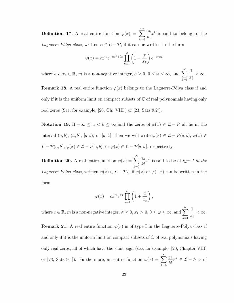
Definition 17. A real entire function ϕ(x) =∞∑

k=0

γk

k!xk is said to belong to the

Laguerre-Polya class, written ϕ ∈ L − P , if it can be written in the form

ϕ(x) = cxme−ax2+bx

ω∏k=1

(1 +

x

xk

)e−x/xk

where b, c, xk ∈ R, m is a non-negative integer, a ≥ 0, 0 ≤ ω ≤ ∞, andω∑

k=1

1

x2k

<∞.

Remark 18. A real entire function ϕ(x) belongs to the Laguerre-Polya class if and

only if it is the uniform limit on compact subsets of C of real polynomials having only

real zeros (See, for example, [20, Ch. VIII ] or [23, Satz 9.2]).

Notation 19. If −∞ ≤ a < b ≤ ∞ and the zeros of ϕ(x) ∈ L − P all lie in the

interval (a, b), (a, b ], [a, b), or [a, b ], then we will write ϕ(x) ∈ L − P(a, b), ϕ(x) ∈

L − P(a, b ], ϕ(x) ∈ L − P [a, b), or ϕ(x) ∈ L − P [a, b ], respectively.

Definition 20. A real entire function ϕ(x) =∞∑

k=0

γk

k!xk is said to be of type I in the

Laguerre-Polya class, written ϕ(x) ∈ L − PI, if ϕ(x) or ϕ(−x) can be written in the

form

ϕ(x) = cxmeσx

ω∏k=1

(1 +

x

xk

),

where c ∈ R, m is a non-negative integer, σ ≥ 0, xk > 0, 0 ≤ ω ≤ ∞, andω∑

k=1

1

xk

<∞.

Remark 21. A real entire function ϕ(x) is of type I in the Laguerre-Polya class if

and only if it is the uniform limit on compact subsets of C of real polynomials having

only real zeros, all of which have the same sign (see, for example, [20, Chapter VIII]

or [23, Satz 9.1]). Furthermore, an entire function ϕ(x) =∞∑

k=0

γk

k!xk ∈ L − P is of

23

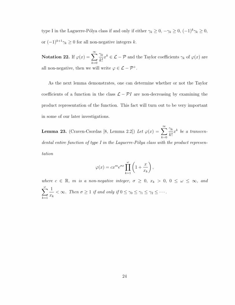
type I in the Laguerre-Polya class if and only if either γk ≥ 0, −γk ≥ 0, (−1)kγk ≥ 0,

or (−1)k+1γk ≥ 0 for all non-negative integers k.

Notation 22. If ϕ(x) =∞∑

k=0

γk

k!xk ∈ L − P and the Taylor coefficients γk of ϕ(x) are

all non-negative, then we will write ϕ ∈ L − P+.

As the next lemma demonstrates, one can determine whether or not the Taylor

coefficients of a function in the class L − PI are non-decreasing by examining the

product representation of the function. This fact will turn out to be very important

in some of our later investigations.

Lemma 23. (Craven-Csordas [8, Lemma 2.2]) Let ϕ(x) =∞∑

k=0

γk

k!xk be a transcen-

dental entire function of type I in the Laguerre-Polya class with the product represen-

tation

ϕ(x) = cxmeσx

ω∏k=1

(1 +

x

xk

),

where c ∈ R, m is a non-negative integer, σ ≥ 0, xk > 0, 0 ≤ ω ≤ ∞, andω∑

k=1

1

xk

<∞. Then σ ≥ 1 if and only if 0 ≤ γ0 ≤ γ1 ≤ γ2 ≤ · · · .

24

Chapter 3

Linear Operators on Real Polynomials

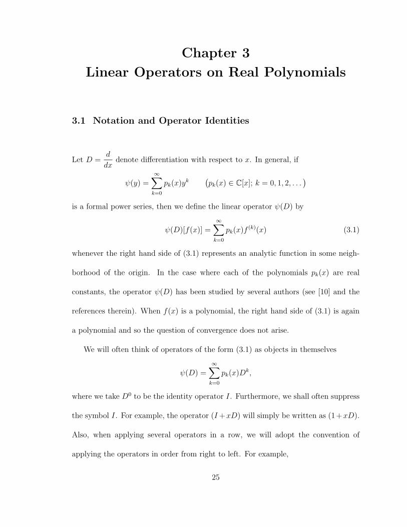
3.1 Notation and Operator Identities

Let D =d

dxdenote differentiation with respect to x. In general, if

ψ(y) =∞∑

k=0

pk(x)yk

(pk(x) ∈ C[x]; k = 0, 1, 2, . . .

)is a formal power series, then we define the linear operator ψ(D) by

ψ(D)[f(x)] =∞∑

k=0

pk(x)f(k)(x) (3.1)

whenever the right hand side of (3.1) represents an analytic function in some neigh-

borhood of the origin. In the case where each of the polynomials pk(x) are real

constants, the operator ψ(D) has been studied by several authors (see [10] and the

references therein). When f(x) is a polynomial, the right hand side of (3.1) is again

a polynomial and so the question of convergence does not arise.

We will often think of operators of the form (3.1) as objects in themselves

ψ(D) =∞∑

k=0

pk(x)Dk,

where we take D0 to be the identity operator I. Furthermore, we shall often suppress

the symbol I. For example, the operator (I+xD) will simply be written as (1+xD).

Also, when applying several operators in a row, we will adopt the convention of

applying the operators in order from right to left. For example,

25

D(x−D)[f(x)] = D[xf(x)− f ′(x)] = xf ′(x) + f(x)− f ′′(x).

This convention is important since, in general, two operators need not commute. For

example, (xD)[f(x)

]= xf ′(x)

while (Dx)[f(x)

]= D

[xf(x)

]= f(x) + xf ′(x). (3.2)

Thus, the operators x = xI and D do not commute. However, equation (3.2)

suggests that the operators Dx and (1 + xD) are actually the same operator. In

general, two operators T1 and T2 are equal if they have the same domain and range

and, for every element v of the domain, T1[v] = T2[v]. We will now demonstrate

equality between certain operators which will be of importance in the sequel.

Lemma 24. For any non-negative integer m and any entire function f(x),

DmxD[f(x)] =(xDm+1 +mDm

)[f(x)], (3.3)

where D denotes differentiation with respect to x.

Proof. From Leibniz’ formula for the nth derivative of the product of two functions

Dn[f(x)g(x)] =n∑

k=0

(n

k

)Dk[f(x)]Dn−k[g(x)],

we have

DmxD[f(x)] = Dm[xf ′(x)] =n∑

k=0

(m

k

)Dk[x]Dm−k[f ′(x)] = xf (m+1)(x) +mf (m)(x).

26

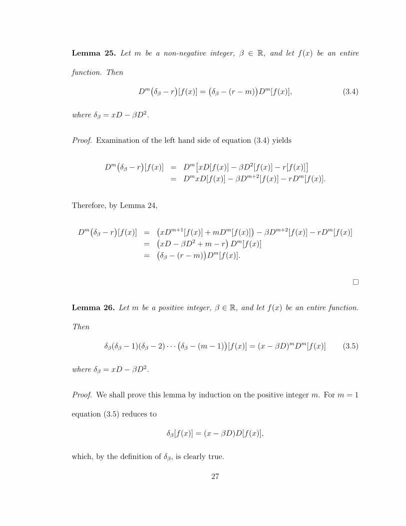
Lemma 25. Let m be a non-negative integer, β ∈ R, and let f(x) be an entire

function. Then

Dm(δβ − r

)[f(x)] =

(δβ − (r −m)

)Dm[f(x)], (3.4)

where δβ = xD − βD2.

Proof. Examination of the left hand side of equation (3.4) yields

Dm(δβ − r

)[f(x)] = Dm

[xD[f(x)]− βD2[f(x)]− r[f(x)]

]= DmxD[f(x)]− βDm+2[f(x)]− rDm[f(x)].

Therefore, by Lemma 24,

Dm(δβ − r

)[f(x)] =

(xDm+1[f(x)] +mDm[f(x)]

)− βDm+2[f(x)]− rDm[f(x)]

=(xD − βD2 +m− r

)Dm[f(x)]

=(δβ − (r −m)

)Dm[f(x)].

Lemma 26. Let m be a positive integer, β ∈ R, and let f(x) be an entire function.

Then

δβ(δβ − 1)(δβ − 2) · · ·(δβ − (m− 1)

)[f(x)] = (x− βD)mDm[f(x)] (3.5)

where δβ = xD − βD2.

Proof. We shall prove this lemma by induction on the positive integer m. For m = 1

equation (3.5) reduces to

δβ[f(x)] = (x− βD)D[f(x)],

which, by the definition of δβ, is clearly true.

27

Now suppose that equation (3.5) holds for some given positive integer m. We first

note that, by taking r = m in Lemma 25,

δβDm[f(x)] = Dm(δβ −m)[f(x)].

Therefore

(x− βD)m+1Dm+1[f(x)] = (x− βD)mδβDm[f(x)]

= (x− βD)mDm(δβ −m)[f(x)]

= δβ(δβ − 1)(δβ − 2) · · · (δβ −m)[f(x)].

Thus the Lemma holds for the integer m+ 1 as well.

Lemma 27. Suppose m ≥ 1 and p ≥ 0 are integers, β ∈ R, and let f(x) be an entire

function. Then

δβ(δβ − 1)(δβ − 2) · · ·(δβ − (m− 1)

) p∏i=1

(δβ − bi)[f(x)]

= (x− βD)m

(p∏

i=1

((m− bi) + xD − βD2

))Dm[f(x)],

where δβ = xD − βD2.

Proof. This is an immediate consequence of equations (3.5) and (3.4) of Lemmas 26

and 25, respectively.

Again, it should be emphasized that the preceding technical lemmas are not that

remarkable in themselves. We have only included them here due to the fact that they

will be of use to us in what follows.

We will now include another result along these lines which is of some significance

in itself. Indeed, the next lemma will be used in one of the major theorems of this

28

dissertation (Theorem 147). Furthermore, it is the result contained in this lemma

which led us to the consideration of the generalized Hermite polynomials Hα defined

by the generating relation (2.11) of the previous chapter.

Lemma 28. For any α ∈ R and any entire function f(x),

(x− αD)k[f(x)] =k∑

j=0

(k

j

)(−α)jH(α)

k−j(x)f(j)(x) (k = 0, 1, 2, . . . ), (3.6)

where D denotes differentiation with respect to x and H(α)n (x) denotes the nth gener-

alized Hermite polynomial defined by the generating relation (2.11).

Proof. If α = 0, then equation (3.6) reduces to

xkf(x) = H(0)k (x)f(x),

which is true since H(0)k (x) = xk.

We will prove that the lemma is true for α 6= 0 by mathematical induction. For

ease of notation, the superscript (α) of H(α)n (x) will be suppressed.

For k = 0, equation (3.6) reduces to

f(x) = H0(x)f(x),

which is true since H0(x) = 1. Suppose that equation (3.6) holds for some given

integer k ≥ 0. Then

(x− αD)k+1[f(x)] = (x− αD)[(x− αD)k[f(x)]

]= (x− αD)

[k∑

j=0

(k

j

)(−α)jHk−j(x)f

(j)(x)

],

which, by the product rule for differentiation, becomes

29

(x− αD)k+1[f(x)] =k∑

j=0

(k

j

)(−α)jxHk−j(x)f

(j)(x)

+k∑

j=0

(k

j

)(−α)j+1

[H′

k−j(x)f(j)(x) +Hk−j(x)f

(j+1)(x)].

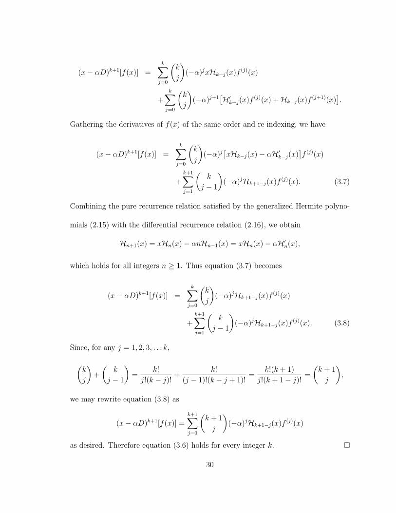
Gathering the derivatives of f(x) of the same order and re-indexing, we have

(x− αD)k+1[f(x)] =k∑

j=0

(k

j

)(−α)j

[xHk−j(x)− αH′

k−j(x)]f (j)(x)

+k+1∑j=1

(k

j − 1

)(−α)jHk+1−j(x)f

(j)(x). (3.7)

Combining the pure recurrence relation satisfied by the generalized Hermite polyno-

mials (2.15) with the differential recurrence relation (2.16), we obtain

Hn+1(x) = xHn(x)− αnHn−1(x) = xHn(x)− αH′n(x),

which holds for all integers n ≥ 1. Thus equation (3.7) becomes

(x− αD)k+1[f(x)] =k∑

j=0

(k

j

)(−α)jHk+1−j(x)f

(j)(x)

+k+1∑j=1

(k

j − 1

)(−α)jHk+1−j(x)f

(j)(x). (3.8)

Since, for any j = 1, 2, 3, . . . k,

(k

j

)+

(k

j − 1

)=

k!

j!(k − j)!+

k!

(j − 1)!(k − j + 1)!=

k!(k + 1)

j!(k + 1− j)!=

(k + 1

j

),

we may rewrite equation (3.8) as

(x− αD)k+1[f(x)] =k+1∑j=0

(k + 1

j

)(−α)jHk+1−j(x)f

(j)(x)

as desired. Therefore equation (3.6) holds for every integer k.

30

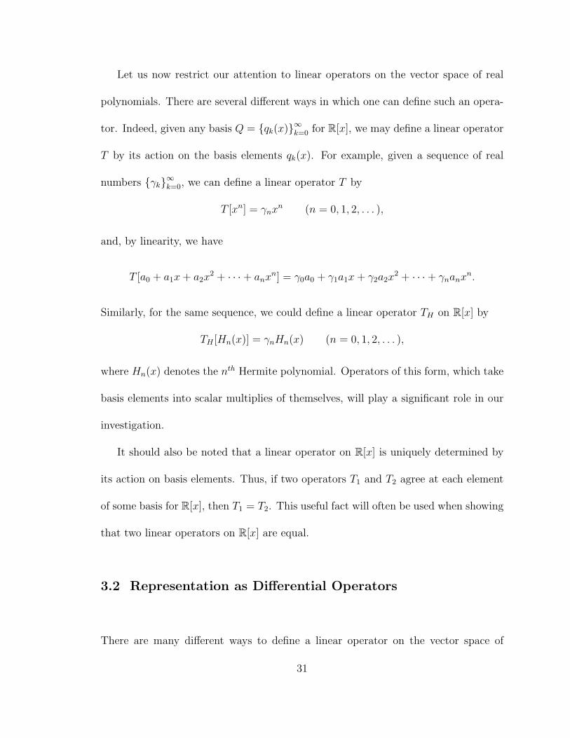
Let us now restrict our attention to linear operators on the vector space of real

polynomials. There are several different ways in which one can define such an opera-

tor. Indeed, given any basis Q = {qk(x)}∞k=0 for R[x], we may define a linear operator

T by its action on the basis elements qk(x). For example, given a sequence of real

numbers {γk}∞k=0, we can define a linear operator T by

T [xn] = γnxn (n = 0, 1, 2, . . . ),

and, by linearity, we have

T [a0 + a1x+ a2x2 + · · ·+ anx

n] = γ0a0 + γ1a1x+ γ2a2x2 + · · ·+ γnanx

n.

Similarly, for the same sequence, we could define a linear operator TH on R[x] by

TH [Hn(x)] = γnHn(x) (n = 0, 1, 2, . . . ),

where Hn(x) denotes the nth Hermite polynomial. Operators of this form, which take

basis elements into scalar multiplies of themselves, will play a significant role in our

investigation.

It should also be noted that a linear operator on R[x] is uniquely determined by

its action on basis elements. Thus, if two operators T1 and T2 agree at each element

of some basis for R[x], then T1 = T2. This useful fact will often be used when showing

that two linear operators on R[x] are equal.

3.2 Representation as Differential Operators

There are many different ways to define a linear operator on the vector space of

31

complex polynomials. In the midst of such variety, it is a remarkable fact that, no

matter how a linear operator T : C[x] → C[x] is defined, it can always be represented

formally as a differential operator with complex polynomial coefficients. The follow-

ing proposition is known but, in the absence of a good reference, we will provide its

proof for the sake of completeness.

Proposition 29. Let T : C[x] → C[x] be a linear operator. Then there exists a

unique set of complex polynomials {pk(x)}∞k=0 such that

T [f(x)] =∞∑

k=0

pk(x)f(k)(x)

for all f(x) ∈ C[x].

Proof. Let T be a linear operator on the set of complex polynomials. Define the

polynomials {pk(x)}∞k=0 recursively by

p0(x) = T [1]

and

pn(x) =1

n!

(T [xn]−

n−1∑k=0

pk(x)Dkxn

)(n = 1, 2, 3, . . . ), (3.9)

where D denotes differentiation with respect to x.

Suppose f(x) =n∑

k=0

akxk is a complex polynomial. Then, by the linearity of T ,

T [f(x)] = T

[n∑

k=0

akxk

]=

n∑k=0

akT[xk]. (3.10)

Furthermore, by equation (3.9),

T[xk]

=k∑

j=0

pj(x)Djxk. (3.11)

Combining equations (3.10) and (3.11) yields

32

T [f(x)] =n∑

k=0

ak

k∑j=0

pj(x)Djxk =

n∑k=0

k∑j=0

akpj(x)Djxk. (3.12)

Since Djxk = 0 for j > k, we may write equation (3.12) as

T [f(x)] =n∑

k=0

n∑j=0

akpj(x)Djxk.

Rewriting this double sum yields

T [f(x)] =n∑

k=0

n∑j=0

akpj(x)Djxk

=n∑

j=0

n∑k=0

akpj(x)Djxk

=n∑

j=0

pj(x)Dj

n∑k=0

akxk

=n∑

j=0

pj(x)f(j)(x)

as desired.

To show that this representation is unique, suppose there exists another set of

complex polynomials {qk(x)}∞k=0 such that

T [f(x)] =∞∑

k=0

qk(x)f(k)(x)

for all f(x) ∈ C[x]. Then, in particular,

n∑k=0

pk(x)Dkxn = T [xn] =

n∑k=0

qk(x)Dkxn (n = 0, 1, 2, . . . ). (3.13)

For n = 0, equation (3.13) becomes p0(x) = q0(x). When n = 1, equation (3.13)

becomes

p0(x)x+ p1(x) = q0(x)x+ q1(x),

33

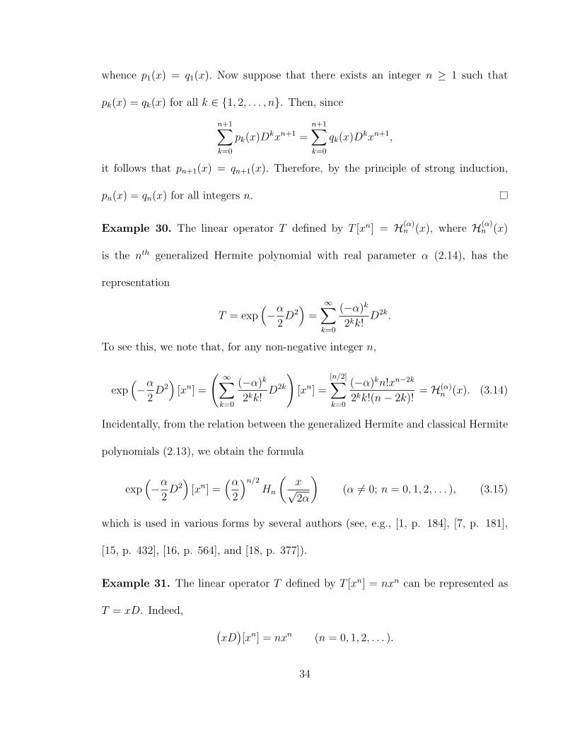
whence p1(x) = q1(x). Now suppose that there exists an integer n ≥ 1 such that

pk(x) = qk(x) for all k ∈ {1, 2, . . . , n}. Then, since

n+1∑k=0

pk(x)Dkxn+1 =

n+1∑k=0

qk(x)Dkxn+1,

it follows that pn+1(x) = qn+1(x). Therefore, by the principle of strong induction,

pn(x) = qn(x) for all integers n.

Example 30. The linear operator T defined by T [xn] = H(α)n (x), where H(α)

n (x)

is the nth generalized Hermite polynomial with real parameter α (2.14), has the

representation

T = exp(−α

2D2)

=∞∑

k=0

(−α)k

2kk!D2k.

To see this, we note that, for any non-negative integer n,

exp(−α

2D2)

[xn] =

(∞∑

k=0

(−α)k

2kk!D2k

)[xn] =

[n/2]∑k=0

(−α)kn!xn−2k

2kk!(n− 2k)!= H(α)

n (x). (3.14)

Incidentally, from the relation between the generalized Hermite and classical Hermite

polynomials (2.13), we obtain the formula

exp(−α

2D2)

[xn] =(α

2

)n/2

Hn

(x√2α

)(α 6= 0; n = 0, 1, 2, . . . ), (3.15)

which is used in various forms by several authors (see, e.g., [1, p. 184], [7, p. 181],

[15, p. 432], [16, p. 564], and [18, p. 377]).

Example 31. The linear operator T defined by T [xn] = nxn can be represented as

T = xD. Indeed, (xD)[xn] = nxn (n = 0, 1, 2, . . . ).

34

Example 32. The linear operator T defined by T [xn] = (1 + n + n2)xn can be

represented as T = 1 + 2xD + x2D2. Indeed,

(1 + 2xD +D2

)[xn] =

(1 + 2n+ n(n− 1)

)xn = (1 + n+ n2)xn (n = 0, 1, 2, . . . ).

In general, the differential operator representation of a linear operator which cor-

responds to a real sequence {γk}∞k=0 has a beautiful representation in terms of the

“reverse” of the Jensen polynomials associated with the sequence.

Proposition 33. Let {γk}∞k=0 be a sequence of real numbers and let

g∗n(x) =n∑

k=0

(n

k

)γkx

n−k (n = 0, 1, 2, . . . ).

Then the linear operator T on the set of real (or complex ) polynomials defined by

T [xn] = γnxn (n = 0, 1, 2, . . . ) can be represented as

T =∞∑

k=0

g∗k(−1)

k!xkDk, (3.16)

where D denotes differentiation with respect to x.

Proof. Let

T =∞∑

k=0

g∗k(−1)

k!xkDk

(D =

d

dx

)be the differential operator which appears in equation (3.16). To show that T = T ,

it suffices to show that

T [xn] = γnxn (n = 0, 1, 2, . . . ). (3.17)

For any integer n ≥ 0,

35

T [xn] =

(∞∑

k=0

g∗k(−1)

k!xkDk

)[xn] =

n∑k=0

n!

(n− k)!

g∗k(−1)

k!xn =

n∑k=0

(n

k

)g∗k(−1)xn.

(3.18)

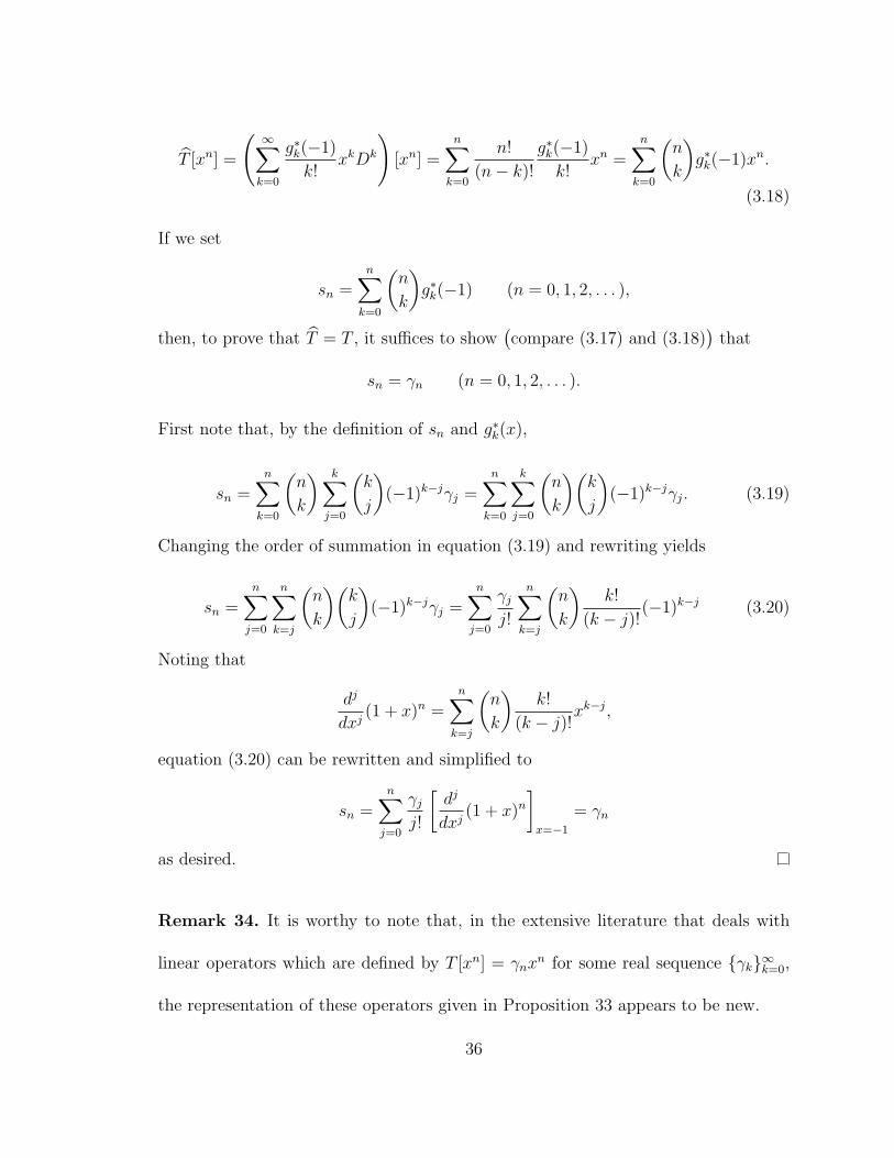
If we set

sn =n∑

k=0

(n

k

)g∗k(−1) (n = 0, 1, 2, . . . ),

then, to prove that T = T , it suffices to show(compare (3.17) and (3.18)

)that

sn = γn (n = 0, 1, 2, . . . ).

First note that, by the definition of sn and g∗k(x),

sn =n∑

k=0

(n

k

) k∑j=0

(k

j

)(−1)k−jγj =

n∑k=0

k∑j=0

(n

k

)(k

j

)(−1)k−jγj. (3.19)

Changing the order of summation in equation (3.19) and rewriting yields

sn =n∑

j=0

n∑k=j

(n

k

)(k

j

)(−1)k−jγj =

n∑j=0

γj

j!

n∑k=j

(n

k

)k!

(k − j)!(−1)k−j (3.20)

Noting that

dj

dxj(1 + x)n =

n∑k=j

(n

k

)k!

(k − j)!xk−j,

equation (3.20) can be rewritten and simplified to

sn =n∑

j=0

γj

j!

[dj

dxj(1 + x)n

]x=−1

= γn

as desired.

Remark 34. It is worthy to note that, in the extensive literature that deals with

linear operators which are defined by T [xn] = γnxn for some real sequence {γk}∞k=0,

the representation of these operators given in Proposition 33 appears to be new.

36

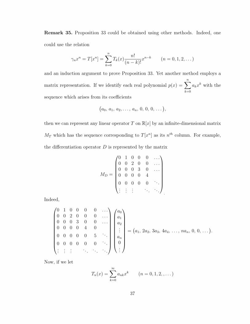
Remark 35. Proposition 33 could be obtained using other methods. Indeed, one

could use the relation

γnxn = T [xn] =

n∑k=0

Tk(x)n!

(n− k)!xn−k (n = 0, 1, 2, . . . )

and an induction argument to prove Proposition 33. Yet another method employs a

matrix representation. If we identify each real polynomial p(x) =n∑

k=0

akxk with the

sequence which arises from its coefficients(a0, a1, a2, . . . , an, 0, 0, 0, . . .

),

then we can represent any linear operator T on R[x] by an infinite-dimensional matrix

MT which has the sequence corresponding to T [xn] as its nth column. For example,

the differentiation operator D is represented by the matrix

MD =

0 1 0 0 0 . . .0 0 2 0 0 . . .0 0 0 3 0 . . .0 0 0 0 4

0 0 0 0 0. . .

......

.... . . . . .

.

Indeed,

0 1 0 0 0 0 . . .0 0 2 0 0 0 . . .0 0 0 3 0 0 . . .0 0 0 0 4 0

0 0 0 0 0 5. . .

0 0 0 0 0 0. . .

......

.... . . . . . . . .

a0

a1

a2...an

0...

=(a1, 2a2, 3a3, 4a4, . . . , nan, 0, 0, . . .

).

Now, if we let

Tn(x) =∞∑

k=0

ankxk (n = 0, 1, 2, , . . . )

37

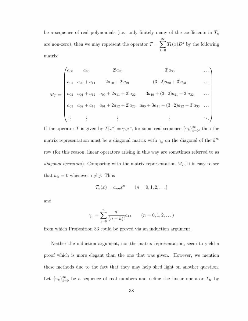
be a sequence of real polynomials (i.e., only finitely many of the coefficients in Tn

are non-zero), then we may represent the operator T =∞∑

k=0

Tk(x)Dk by the following

matrix.

MT =

a00 a10 2!a20 3!a30 . . .

a01 a00 + a11 2a10 + 2!a21 (3 · 2)a20 + 3!a31 . . .

a02 a01 + a12 a00 + 2a11 + 2!a22 3a10 + (3 · 2)a21 + 3!a32 . . .

a03 a02 + a13 a01 + 2a12 + 2!a23 a00 + 3a11 + (3 · 2)a22 + 3!a33 . . .

......

......

. . .

If the operator T is given by T [xn] = γnx

n, for some real sequence {γk}∞k=0, then the

matrix representation must be a diagonal matrix with γk on the diagonal of the kth

row (for this reason, linear operators arising in this way are sometimes referred to as

diagonal operators). Comparing with the matrix representation MT , it is easy to see

that aij = 0 whenever i 6= j. Thus

Tn(x) = annxn (n = 0, 1, 2, . . . )

and

γn =n∑

k=0

n!

(n− k)!akk (n = 0, 1, 2, . . . )

from which Proposition 33 could be proved via an induction argument.

Neither the induction argument, nor the matrix representation, seem to yield a

proof which is more elegant than the one that was given. However, we mention

these methods due to the fact that they may help shed light on another question.

Let {γk}∞k=0 be a sequence of real numbers and define the linear operator TH by

38

TH [Hn(x)] = γnHn(x), where Hn is the nth Hermite polynomial. By Proposition 29,

this operator may be represented in the form

TH =∞∑

k=0

Tk(x)Dk

(Tk ∈ R[x]

).

The question is whether or not there is an explicit formula which defines the polyno-

mials Tk in this representation. If such a formula exists, the formula for the product

of two Hermite polynomials (2.10) is undoubtedly relevant.

3.3 Linear Operators Which Preserve Reality of Zeros

Although the following terminology is not standard, we shall use it due to its in-

tuitive nature.

Definition 36. A linear operator T : R[x] −→ R[x] is said to preserve reality of zeros

if it has the property that

T [p(x)] ∈ L − P whenever p(x) ∈ (R[x] ∩ L − P) . (3.21)

Thus, T preserves reality of zeros if and only if T maps polynomials with only real

zeros to polynomials with only real zeros or, perhaps, to the identically zero function.

For example, as a consequence of Rolle’s theorem, the differentiation operatorD =d

dx

preserves reality of zeros. More generally, if p(x) ∈ R[x] has only real zeros, then the

operator p(D) preserves reality of zeros, which is a consequence of the well-known

Hermite-Poulain Theorem.

39

Theorem 37. (Hermite-Poulain Theorem [20, p. 337], [23, p. 4]) Let

h(x) = c0 + c1x+ c2x2 + · · ·+ cnx

n

be a real polynomial with only real zeros. Then, for any real polynomial f(x), the

number of non-real zeros of

h(D)f(x) = c0f(x) + c1f′(x) + c2f

′′(x) + · · ·+ cnf(n)(x)

does not exceed the number of non-real zeros of f(x).

The most elegant proof of this theorem is again due to Rolle’s theorem. Indeed, the

operator h(D) can be factored into operators of the form α+D and

d

dx

(eαxf(x)

)=(αf(x) + f ′(x)

)eαx.

As the next theorem demonstrates, one can actually take h(x) in the Hermite-Poulain

Theorem to be a transcendental function in the class L − P . This important fact will

be useful to us in our later investigations.

Theorem 38. Let

ϕ(x) =∞∑

k=0

akxk ∈ L − P .

Then, for any real polynomial f(x), the number of non-real zeros of

ϕ(D)[f(x)] =∞∑

k=0

akf(k)(x)

does not exceed the number of non-real zeros of f(x).

Proof. Since ϕ(x) ∈ L − P , there is a sequence of polynomials

pm(x) =nm∑k=0

am,kxk (m = 1, 2, 3, . . . ),

40

each of which has only real zeros, which converge uniformly on compact subsets of C

to ϕ(x). The coefficients of pm(x) tend to those of ϕ(x), i.e.,

limm→∞

am,k = ak (k = 0, 1, 2, . . . ).

Thus, for any real polynomial f(x), the sequence of polynomials {pm(D)[f(x)]}∞m=1

converge uniformly on compact subsets to ϕ(D)[f(x)]. Therefore, by the Hermite-

Poulain Theorem and Hurwitz’ theorem (see Corollary 12), the number of non-real

zeros of ϕ(D)[f(x)] does not exceed the number of non-real zeros of f(x).

One of the fundamental results which gives rise to linear operators which preserve

reality of zeros is is the following composition theorem.

Theorem 39. (Schur-Malo Composition Theorem [12, p. 7],[20, pp. 337-340]) Sup-

pose that all the zeros of the polynomial p(x) =m∑

k=0

akxk (am 6= 0) are real and all

zeros of the polynomial q(x) =n∑

k=0

bkxk (bn 6= 0) are real and of the same sign. If we

set ν = min{m,n}, then all of the zeros of the polynomials f(x) =ν∑

k=0

k!akbkxk and

g(x) =ν∑

k=0

akbkxk are also real.

The composition theorem provides a powerful tool in studying the diagonal operators,

i.e., operators defined by T [xn] = γnxn for some real sequence {γk}∞k=0, which preserve

reality of zeros. The sequences which give rise to these operators are called multiplier

sequences. To be precise, we have the following definition.

Definition 40. A sequence of real numbers {γk}∞k=0 is called a multiplier sequence if

the corresponding linear operator T , defined by T [xn] = γnxn, has the property that

41

T [p(x)] ∈ L − P whenever p(x) ∈ (R[x] ∩ L − P) .

Let us begin the discussion of multiplier sequences with some introductory examples.

Example 41. Fix a non-zero real number r and define the linear operator T by

T [xn] = rnxn. If p(x) is a real polynomial having only real zeros, then T [p(x)] = p(rx)

also has only real zeros. Thus, for any non-zero real number r, the geometric sequence{rk}∞

k=0is a multiplier sequence.

Example 42. Another elementary example of a multiplier sequence is the sequence

{k}∞k=0. To see this, we only need to note that, for every non-negative integer n,

(xD)[xn] = nxn, and the operator xD preserves reality of zeros.

In order to demonstrate a more interesting example of a multiplier sequence, we prove

the following lemma.

Lemma 43. Suppose that the complex polynomial

f(x) = a0 + a1x+ a2x2 + · · ·+ anx

n (an 6= 0)

has only real zeros. Then the complex polynomial

f ∗(x) = a0xn + a1x

n−1 + a2xn−2 + · · ·+ an

also has only real zeros.

Proof. The lemma is a consequence of the relation

f ∗(x) = xnf

(1

x

).

42

Example 44. The sequence

{1

k!

}∞k=0

is a multiplier sequence. Indeed, if p(x) =

n∑k=0

akxk has only real zeros, then the same is true of the polynomial p∗(x) =

n∑k=0

akxn−k.

Thus, by the Hermite-Poulain Theorem,

p∗(D)

[xn

n!

]=

n∑k=0

ak

k!xk

has only real zeros.

Before citing more examples, we will give several properties of multiplier sequences

which are readily verified.

Proposition 45. ([9], [20, p. 341]) Let {γk}∞k=0 be a multiplier sequence. Then

1. The sequence {γk}∞k=m is also a multiplier sequence, where m is any non-negative

integer.

2. If there exists an integer m ≥ 0 such that γm 6= 0 and an integer n > m such

that γn = 0, then γk = 0 for all k ≥ n.

3. The elements of {γk}∞k=0 are either all of the same sign, or they alternate in

sign.

4. The sequence{(−1)kγk

}∞k=0

is also a multiplier sequence.

5. For any r ∈ R, the sequence {rγk}∞k=0 is also a multiplier sequence.

6. The elements of {γk}∞k=0 satisfy Turan’s inequality

γ2k − γk−1γk+1 ≥ 0 (k = 1, 2, 3, . . . ).

43

In 1883, Laguerre [19] proved that the sequences

{1,

1

α+ ω,

1

(α+ ω)(2α+ ω),

1

(α+ ω)(2α+ ω)(3α+ ω), . . .

}(α, ω > 0)

and {1, q, q4, q9, . . . , qn2

, . . .}

(−1 ≤ q ≤ 1)

are multiplier sequences. In 1911, Jensen([17], [20, p. 343]

)invoked the Schur-Malo

Composition Theorem to show that, for any positive integer n, the sequence

{1, 1,

(1− 1

n

), . . . ,

(1− 1

n

)(1− 2

n

)· · ·(

1− n− 1

n

), 0, 0, 0, . . .

}

is a multiplier sequence. In 1914, Polya and Schur completely characterized multiplier

sequences as follows.

Theorem 46. (Polya-Schur [26], [20, Chapter VIII], [23, Kapitel II]) Let {γk}∞k=0

be a sequence of non-negative real numbers and let T be the linear operator on R[x]

defined by T [xn] = γnxn. Then the following are equivalent.

1. {γk}∞k=0 is a multiplier sequence.

2. (Transcendental Characterization)

T [ex] =∞∑

k=0

γk

k!xk ∈ L − P+.

3. (Algebraic Characterization) For each n = 0, 1, 2, . . .

T [(1 + x)n] =n∑

k=0

(n

k

)γkx

k ∈ L − P+.

44

Although the preceding theorem only applies to non-negative sequences, Properties

3-5 of Proposition 45 complete the characterization of multiplier sequences.

Until now, all linear operators have been only defined on vector spaces which

consist of polynomials. However, the Transcendental Characterization of multiplier

sequences in Theorem 46 requires that we be able to apply the multiplier sequence

to the Taylor coefficients of the transcendental entire function ex. The next theorem

shows that it does, in fact, make sense to apply a multiplier sequence to any function

in the Laguerre-Polya class.

Theorem 47. ([20, p. 343]) Suppose {γk}∞k=0 is a multiplier sequence and let T be

the corresponding operator defined by T [xn] = γnxk. If f(x) =

∞∑k=0

akxk ∈ L − P,

then the function T [f(x)] =∞∑

k=0

akγkxk represents an entire function, and this entire

function also belongs to the Laguerre-Polya class.

Let us now employ Polya and Schur’s characterization to give an example of a

multiplier sequence which will be of great interest to us later on.

Example 48. The sequence{1 + k + k2

}∞k=0

is a multiplier sequence. Let us first

show this using the algebraic characterization of multiplier sequences given in Theo-

rem 46. Let T be the linear operator defined by T [xn] = (1 + n + n2)xn. Then the

differential operator representation of T is T = 1+2xD+D2, which follows from the

relation (1 + 2xD + x2D2

)[xn] = (1 + n+ n2)xn (n = 0, 1, 2, . . . ).

Thus,

45

T[(x+ 1)n

]=

(1 + 2xD + x2D2

)[(1 + x)n

]= (x+ 1)n−2

((n2 + n+ 1)x2 + 2(n+ 1)x+ 1

). (3.22)

And, since the discriminant of the quadratic polynomial in equation (3.22) is 4n ≥ 0,

T[(x + 1)n

]has only real zeros for any integer n ≥ 0. Therefore, the sequence{

1 + k + k2}∞

k=0is a multiplier sequence.

Alternatively, we could use the transcendental characterization of multiplier se-

quences given in Theorem 46. Since

ϕ(x) =∞∑

k=0

1 + k + k2

k!xk = (x+ 1)2ex ∈ L − P+,

the sequence{1 + k + k2

}∞k=0

is a multiplier sequence.

To cite a result regarding linear operators which arise from applying a given real

sequences to a basis other than the standard basis{xk}∞

k=0, we have the following

classical result which Turan announced in 1950.

Theorem 49. (Turan [29, p. 289], [1, p. 178]) Suppose the real polynomialn∑

k=0

akHk(x),

where Hk denotes the kth Hermite polynomial, has only real zeros. If g(x) is a poly-

nomial having only real negative zeros, then the polynomialn∑

k=0

akg(k)Hk(x) also has

only real zeros.

In 2001 Bleecker and Csordas [1, Theorem 2.7] proved and generalized this result.

They demonstrated that one can take g(x) to be any transcendental function in the

class L − P+. Their investigations led them to state the following open problem.

46

Problem 50. (Bleecker-Csordas [1, Problem 4.1]) Characterize all real sequences

{γk}∞k=0 such that

ifn∑

k=0

akHk(x) ∈ L − P , thenn∑

k=0

γkakHk(x) ∈ L − P , (3.23)

where Hk denotes the kth Hermite polynomial.

Remark 51. Problem 50 was the source of inspiration for a large portion of the

research contained in this dissertation, and we shall see its complete solution in the

chapters which follow.

It is worthy to note that Bleecker and Csordas were able to generalize Turan’s

theorem by discovering another linear operator on R[x] which preserves reality of

zeros.

Proposition 52. (Bleecker-Csordas [1, Lemma 2.2]) Suppose that the real polynomial

p(x) has only real zeros. Then, for any fixed α ≥ 0 and β ≥ 0,

f(x) = αp(x) + xp′(x)− βp′′(x) ∈ L − P .

Remark 53. Proposition 52 states that, for any non-negative constants α and β,

the operator α + xD − βD2 preserves reality of zeros. Operators of this form arise

naturally in connection with the Hermite polynomials. Indeed, since the Hermite

polynomials satisfy Hermite’s differential equation (2.7) we have(xD − 1

2D2

)[Hn(x)] = nHn(x) (n = 0, 1, 2, . . . ). (3.24)

By iterating relation (3.24) we see that, for any entire function g(x),

47

g

(xD − 1

2D2

)[Hn(x)] = g(n)Hn(x) (n = 0, 1, 2, . . . ). (3.25)

Thus, Turan’s theorem (Theorem 49) follows immediately from relation (3.25) and

Proposition 52.

In the next section we will show that operators of the form α + xD − βD2, with

α, β ≥ 0, satisfy another property which is stronger than the property of preserving

reality of zeros. We will also show that, under certain restrictions on the degree of

the polynomial p(x), we may replace the term xp′(x) of f(x) in Proposition 52 by

the term (cx + d)p′(x), where c and d are real constants. These generalizations will

provide a way to further generalize Turan’s theorem (Theorem 49).

To conclude this section, we mention a very recent result which completely char-

acterizes linear operators which preserve reality of zeros in terms of the distribution of

zeros of certain functions in two variables. Given a linear operator T : R[x] −→ R[x],

we extend the operator to the vector space R[x, y] by declaring T [xnym] = ymT [xn]

for all non-negative integers n and m. Thus the extension is obtained by essentially

treating the second variable as a scalar. In 2006, Borcea, Branden and Shapiro [2]

used this extension to establish an algebraic characterization of linear operators which

preserve reality of zeros.

Theorem 54. (Borcea, Branden and Shapiro [2, Corollary 1]) A linear operator

T : R[x] −→ R[x] preserves reality of zeros if and only if either

(a) T has range of dimension no greater than two and is of the form

48

T [f(x)] = α(f(x))P (x) + β(f(x))Q(x),

where α and β are linear functionals on R[x] and P (x) and Q(x) are real poly-

nomials which have only real zeros which interlace, or

(b) Each of the polynomials in one of the sets {T [(x+ y)n]}∞n=0 or {T [(x− y)n]}∞n=0

do not have any zeros in the set H = {(x, y) ∈ C2 : Im(x) > 0, Im(y) > 0}.

In the same paper, Borcea, Branden and Shapiro also gave the following transcen-

dental characterization of linear operators which preserve reality of zeros.

Theorem 55. (Borcea, Branden and Shapiro [2, Theorem 5]) A linear operator T :

R[x] −→ R[x] preserves reality of zeros if and only if either

(a) T has range of dimension no greater than two and is of the form

T [f(x)] = α(f(x))P (x) + β(f(x))Q(x),

where α and β are linear functionals on R[x] and P (x) and Q(x) are real poly-

nomials which have only real zeros which interlace, or

(b) One of the expressions∞∑

k=0

(−y)k

k!T [xk] or

∞∑k=0

(−y)k

k!T [−xk] represents an en-

tire function in two variables which is the uniform limit on compact subsets of

polynomials which do not have any zeros in the set

H = {(x, y) ∈ C2 : Im(x) > 0, Im(y) > 0}. (3.26)

49

While these characterizations are quite amazing, they can be difficult to apply in

practice. In general, it seems to be rather difficult to determine whether or not a

polynomial in two variables has all its zeros outside of the set (3.26).

3.4 Complex Zero Decreasing Operators

In what follows, we will often be counting non-real zeros of a given function. To

facilitate the discussion, we will adopt the following notation.

Notation 56. For any entire function f(x), which is not identically zero, let ZC

(f(x)

)denote the number of non-real zeros of f(x), counting multiplicities. For convenience,

we shall also define ZC(0) = 0.

Again, the following terminology is not standard, but we shall use it due to its intuitive

nature.

Definition 57. A linear operator T : R[x] −→ R[x] is called a complex zero decreasing

operator if it has the property that, for every real polynomial p(x),

ZC

(T [p(x)]

)≤ ZC

(p(x)

). (3.27)

Thus, T is a complex zero decreasing operator if and only if T does not increase the

number of non-real zeros of any real polynomial (except, possibly, for real polynomials

which it takes to the identically zero function). In particular, every complex zero

decreasing operator must also preserve reality of zeros.

50

We saw in the previous section that the differentiation operator D =d

dxpreserves

reality of zeros. In fact, the differentiation operator is a complex zero decreasing

operator, which follows from Rolle’s theorem. More generally, by the Hermite-Poulain

Theorem (Theorem 37), if p(x) is a real polynomial with only real zeros, then p(D)

is a complex zero decreasing operator.

The subclass of diagonal complex zero decreasing operators, which are defined by

T [xn] = γnxn for some real sequence {γk}∞k=0, have been studied by several authors.

In analogy to multiplier sequences, the following definition is commonly used.

Definition 58. A sequence of real numbers {γk}∞k=0 is called a complex zero de-

creasing sequence, or CZDS for brevity (which we will also use in the plural), if the

corresponding linear operator T , defined by T [xn] = γnxn, has the property that, for

every real polynomial p(x),

ZC

(T [p(x)]

)≤ ZC

(p(x)

).

Remark 59. It easy to see that the sequences{rk}∞

k=0and {k}∞k=0 of Examples

41 and 42, respectively, are CZDS. However, whether or not the sequence

{1

k!

}∞k=0

of Example 44 is a CZDS is not so clear. Perhaps the Hermite-Poulain Theorem

could be adapted to handle polynomials which do not necessarily have only real

zeros. In particular, it would be desirable to know that, if the real polynomial p

has 2d non-real zeros, then p(D) will not increase the number of non-real zeros of

any real polynomial by more than 2d. However this is not the case. For example, if

p(x) = x2+1 and q(x) = (x2−4)(x2−9). Then ZC

(q(x)

)= 0, while ZC

(p(D)[q(x)]

)=

51

ZC(x4 − x2 + 10) = 4. Thus, the operator p(D) has increased the number of non-

real zeros of q by four, while p(x) only has two non-real zeros. As it turns out, the

sequence

{1

k!

}∞k=0

is a CZDS. This is a consequence of a theorem due to Laguerre

which was subsequently extended by Polya [24].

Theorem 60. (Laguerre’s Theorem [23, p. 6], [12, p. 23])

1. Let f(x) =n∑

k=0

akxk be an arbitrary real polynomial of degree n and let h(x) be

a polynomial with only real zeros, none of which lie in the interval (0, n). Then

ZC

(n∑

k=0

h(k)akxk

)≤ ZC

(f(x)

).

2. Let f(x) =n∑

k=0

akxk be an arbitrary real polynomial of degree n, let ϕ(x) ∈

L − P, and suppose that none of the zeros of ϕ lie in the interval (0, n). Then

ZC

(n∑

k=0

ϕ(k)akxk

)≤ ZC

(f(x)

).

3. If ϕ ∈ L − P(−∞, 0], then the sequence {ϕ(k)}∞k=0 is a CZDS.

Example 61. Since1

Γ(x+ 1)∈ L − P(−∞, 0], where Γ(x) denotes the Gamma

function, the sequence {1

Γ(k + 1)

}∞k=0

=

{1

k!

}∞k=0

is a CZDS.

Let us now demonstrate that there are non-trivial CZDS which cannot be inter-

polated by functions in L − P+.

52

Example 62. For any integer m ≥ 2, the sequence {k(k − 1) · · · (k −m+ 1)}∞k=0 is

a CZDS. To see this, we only need to note that(xmDm

)[xn] = n(n− 1) · · · (n−m+ 1)xn (n = 0, 1, 2, . . . ),

and the operator xnDn is, by Rolle’s theorem, a complex zero decreasing operator. If

there were a function

ϕ(x) =∞∑

k=0

akxk ∈ L − P+ (ak ≥ 0; k = 0, 1, 2, . . . )

which interpolated the sequence {k(k − 1) · · · (k −m+ 1)}∞k=0, then, in particular, we

have

0 = ϕ(1) =∞∑

k=0

ak (ak ≥ 0; k = 0, 1, 2, . . . ).

Therefore, ak = 0 for all k, but this contradicts the fact that ϕ(m) = m! 6= 0. Whence,

for any m ≥ 2, the CZDS {k(k − 1) · · · (k −m+ 1)}∞k=0 cannot be interpolated by a

function in L − P+.

Part 1 of Laguerre’s theorem asserts that any sequence which can be interpolated

by a real polynomial which has only real negative zeros is a CZDS. It turns out that

the converse is true under the additional hypothesis that the interpolating polynomial

does not vanish at the origin. In the case where the interpolating polynomial does

vanish at the origin, it turns out that the sequence must be of a special form related to

Example 62. The following characterization of polynomials which interpolate CZDS

was given by Craven and Csordas in 1991.

53

Theorem 63. (Craven-Csordas [11, p. 13]) Let h(x) be a real polynomial. Then

{h(k)}∞k=0 is a CZDS if and only if either

1. h(0) 6= 0 and h(x) has only real negative zeros, or

2. h(0) = 0 and h(x) is of the form

h(x) = x(x− 1)(x− 2) · · · (x−m+ 1)

p∏k=1

(x− bk)

where m ≥ 1 and p ≥ 0 are integers and bk < m for k = 1, 2, 3, . . . , p.

It is now easy to demonstrate the existence of a multiplier sequence (see Example

48) which is not a CZDS.

Example 64. The multiplier sequence{1 + k + k2

}∞k=0

is not a CZDS. Indeed, this

sequence can be interpolated by the polynomial h(x) = 1+x+x2 which has two non-

real zeros. Therefore, by Theorem 63, this sequence is not a CZDS. Alternatively, if

the linear operator T is defined by T [xn] = (1 + n+ n2)xn then, as was noted in [11,

p. 5], the polynomial

p(x) = (x+ 1)6

(x2 +

1

2x+

1

5

)has two non-real zeros, while the polynomial

T [p(x)] =1

10(x+ 1)4

(730x4 + 785x3 + 306x2 + 43x+ 2

)has four non-real zeros. This concrete example demonstrates, again, that the sequence{1 + k + k2

}∞k=0

is not a CZDS.

54

It should be noted that, in contrast to multiplier sequences, there is no complete

characterization of CZDS. Indeed, the following tantalizing problem remains open.

Problem 65. ([12, p. 26]) Is{e−k3

}∞k=0

a CZDS?

In the previous section, Turan’s theorem (Theorem 49) gave an example of linear

operators, each of which preserves reality of zeros, which are defined by applying the

elements of a real sequence to a basis other than the standard basis{xk}∞

k=0. In

general, there does not seem to be any known results in this direction for complex

zero decreasing operators. Thus the following problem remains open for all choices

of Q, and very little is known if Q is not the standard basis.

Problem 66. Let Q = {qk(x)}∞k=0 be a basis for the vector space of real polynomials

R[x]. Can one characterize the real sequences {γk}∞k=0 which have the property that,

for any real polynomialn∑

k=0

akqk(x),

ZC

(n∑

k=0

akγkqk(x)

)≤ ZC

(n∑

k=0

akqk(x)

)? (3.28)

In order to demonstrate the existence of non-trivial sequences with this property for

the Hermite basis {Hk(x)}∞k=0, we will need to generalize a result of Bleecker and

Csordas mentioned in the previous section (Proposition 52). The generalization will

require the following lemma, which is itself a generalization of a lemma used by Craven

and Csordas [10, Lemma 3.8].

Lemma 67. Suppose that p(x) is a real polynomial of degree n. If c, d, β are real

numbers such that c ≥ 0 and β ≥ 0, then ZC

(q(x)

)≤ ZC

(p(x)

), where

55

q(x) = (cx+ d)p(x)− βp′(x). (3.29)

Proof. The lemma is clearly true when β = 0. If c = 0, then the lemma is an

immediate consequence of the Hermite-Poulain Theorem (Theorem 37).

Suppose β > 0 and c > 0 and let m be the number of real zeros of p(x) counting

multiplicities, i.e.,

ZC

(p(x)

)= n−m

(n = deg(p)

). (3.30)

We may write the polynomial q(x) of (3.29) in the form

q(x) = −β exp

(c

2βx2 +

d

βx

)d

dx

[exp

(− c

2βx2 − d

βx

)p(x)

].

Thus, the zeros of q(x) coincide with the zeros of f ′(x), where we define f(x) by

f(x) = exp

(− c

2βx2 − d

βx

)p(x). (3.31)

Furthermore, the zeros of f(x) coincide with the zeros of p(x). Let x1 and x2 denote

the smallest and largest of the zeros of f(x), respectively. Then, as a consequence of

Rolle’s theorem (see Corollary 7), f ′(x) has at least m − 1 real zeros in the interval

[x1, x2]. Furthermore, f(x) vanishes at x1 and x2, has constant sign on each of the

unbounded intervals (−∞, x1) and (x2,∞), and tends to zero as x→ ±∞. Therefore,

f ′(x) must have at least one zero in each of these unbounded intervals. Whence, f ′(x)

has at least (m−1)+2 = m+1 real zeros. Noting that deg(q) = deg(p)+1, we have

ZC

(q(x)

)= ZC

(f ′(x)

)≤ (n+ 1)− (m+ 1) = n−m = ZC

(p(x)

).

56

We are now in a position to generalize Proposition 52.

Proposition 68. Suppose

p(x) =n∑

k=0

akxk (an 6= 0)

is a real polynomial. If α, β, c, d are real numbers such that α ≥ 0, β ≥ 0, and

α+ cn ≥ 0, then ZC

(f(x)

)≤ ZC

(p(x)

), where

f(x) = αp(x) + (cx+ d)p′(x)− βp′′(x).

Proof. If α = 0, then the condition α + nc ≥ 0 implies that c ≥ 0. Thus, by Lemma

67 and Rolle’s theorem,

ZC

(f(x)

)= ZC

((cx+ d)p′(x)− βp′′(x)

)≤ ZC

(p′(x)

)≤ ZC

(p(x)

).

Now suppose α > 0. We will first consider the case where each of the real zeros of

the polynomial p(x) are simple. Suppose p(x) has exactly m real (simple) zeros, i.e.,

ZC

(p(x)

)= n−m

(n = deg(p)

).

Since deg(f) ≤ deg(p) = n, we have ZC(f) ≤ n. Thus the proposition is true when

m = 0. If m = 1, then, either deg(f) < deg(p), or f(x) is of odd degree and, therefore,

has at least one real zero. In either case, ZC

(f(x)

)≤ n− 1 = ZC

(p(x)

), and so the

proposition is also true in this case. We may, therefore, assume that m ≥ 2.

Denote the real zeros of p(x) by x1 < x2 < x3 < · · · < xm. By Rolle’s theorem,

for each i = 1, 2, 3, . . . ,m− 1, p′(x) has at least one real zero in each of the intervals

(xi, xi+1). For each i = 1, 2, 3, . . . ,m − 1, let yi denote the smallest zero of p′(x) in

the interval (xi, xi+1). To help clarify this notation, we remark that

57

x1 < y1 < x2 < y2 < · · · < xm−1 < ym−1 < xm.

In particular, we have p(yi) 6= 0 for i = 1, 2, 3, . . . ,m − 1. Furthermore, the signs of

the sequence{p(y1), p(y2), p(y3), . . . , p(ym−1)

}alternate.

Fix an integer i ∈ {1, 2, 3, . . . ,m − 1}. We will demonstrate that f(yi) 6= 0 and

that the sign of f(yi) is the same as the sign of p(yi). First note that, since xi is a

simple zero of p(x), we have p′(xi) 6= 0. Since we have chosen yi to be the smallest

zero of p′(x) in the interval (xi, xi+1), we know that p′(x) has constant sign on [xi, yi).

Furthermore, since

p′(xi) = limx→x+

i

p(x)− p(xi)

x− xi

= limx→x+

i

p(x)

x− xi

,

we have that p(x) and p′(x) have the same sign on the interval (xi, yi). It follows

that

p(yi)p′′(yi) = p(yi) lim

x→y−i

p′(x)− p′(yi)

x− yi

= limx→y−i

p(yi)p′(x)

x− yi

≤ 0. (3.32)

Therefore, since we have assumed α > 0 and β ≥ 0, and since we have chosen yi so

that p(yi) 6= 0 and p′(yi) = 0,

f(yi) = αp(yi) + (cyi + d)p′(yi)− βp′′(yi) = αp(yi)− βp′′(yi) 6= 0

and

sign[f(yi)

]= sign

[p(yi)

](i = 1, 2, 3, . . .m− 1). (3.33)

Thus the signs of the sequence{f(y1), f(y2), f(y3), . . . , f(ym−1)

}alternate, and, therefore, f(x) has at least m− 2 zeros in the interval (y1, ym−1).

58

Note that the coefficient of xn in the polynomial f(x) is equal to (α+cn)an, where

an is the leading coefficient of p(x). If α+ cn = 0, then deg(f) ≤ n− 1. Thus, in this

case,

ZC

(f(x)

)≤ (n− 1)− (m− 2) = n−m+ 1.

But, since non-real zeros of a real polynomial come in pairs, we know that ZC

(p)

=

m−n is even. Similarly, ZC

(f(x)

)is also even and, therefore, cannot equal n−m+1.

I.e., in the case where α+ cn = 0, we have shown that ZC

(f(x)

)≤ m− n.

Now suppose α + cn > 0. We will demonstrate that f(x) has a zero in the

unbounded interval (ym−1,∞). Without loss of generality, suppose that the leading

coefficient an of p(x) is positive. Then p(ym−1) < 0 and, by relation (3.33), f(ym−1) <

0. Since the leading coefficient (α + cn)an is also positive, f(x) → ∞ as x → ∞.

Therefore, f(x) has a zero in the interval (yi+1,∞). Whence

ZC

(f(x)

)≤ n− (m− 1) = n+m+ 1,

and, taking into account the parity of the number of non-real zeros of a real poly-

nomial, we have ZC

(f(x)

)≤ m − n = ZC

(p(x)

). It should be noted that one could

prove the existence of an additional zero in the other unbounded interval (−∞, y1).

We have now proved that the proposition is valid when all of the real zeros of p(x)

are simple.

In general, suppose p(x) has m real zeros x1 ≤ x2 ≤ x3 ≤ · · · ≤ xm, which are not

necessarily distinct, and 2N non-real zeros {νk ± iµk}Nk=1. Then, for ε > 0, we form

the polynomial

59

pε(x) = an

[m∏

k=1

(x− (xk + kε)

)] [ N∏k=1

((x− νk)

2 + µ2k

)]

and set

fε(x) = αpε(x) + (cx+ d)p′ε(x)− βp′′ε (x).

For each ε > 0, all of the real zeros of pε are simple. Thus

ZC

(fε(x)

)≤ ZC

(pε(x)

)= 2N (ε > 0).

The sequence of functions{f1/k(x)

}∞k=1

converge uniformly on compact subsets of C

to f(x) and, by Hurwitz’ theorem,

ZC

(f(x)

)≤ 2N = ZC

(p(x)

).

In particular, Proposition 68 states that the linear operator

α+ xD − βD2 (α ≥ 0, β ≥ 0)

is a complex zero decreasing operator. We shall use this fact to further generalize

Turan’s theorem (Theorem 49), but we will postpone this discussion until the next

chapter.

Before moving on, it is also worth mentioning another class of complex zero de-

creasing operators which were studied by Carnicer, Pena, and Pinkus [7] in 2002.

They studied linear operators defined by

T [xn] = xn +n−1∑k=0

bn,kxn (bn,k ∈ R; n = 0, 1, 2, . . . ) (3.34)

and completely characterized all complex zero decreasing operators of this form.

60

Theorem 69. (Carnicer, Pena, Pinkus [7, p. 5]) Let the linear operator T be defined

by (3.34). Then T is a complex zero decreasing operator if and only if T = F (D),

where F (x) ∈ L − P and F (0) = 1.

Thus, Carnicer, Pena, and Pinkus characterized complex zero decreasing operators

whose corresponding matrix representation (see Remark 35) is unitary upper trian-

gular, i.e., of the form

MT =

1 b1,0 b2,0 b3,0 b4,0 . . .0 1 b2,1 b3,1 b4,1 . . .0 0 1 b3,2 b4,2 . . .0 0 0 1 b4,3

0 0 0 0 1. . .

......

.... . . . . .

.

However, this class of operators is not applicable to our current investigation since it

does not include any of the operators involved in Problem 66 except, of course, the

identity operator.

3.5 Extension to Transcendental Entire Functions

Up to now, we have mostly considered linear operators which act on the vector

space of real polynomials. In this section, we will consider linear operators which

act on transcendental entire functions and, whenever possible, extend the results of

the previous sections. In this setting, we must use caution as the issue of convergence

often arises. For example, the infinite order differential operator∞∑

k=0

Dk presents no

problem when applied to polynomials. However, if r > 1 then

61

(∞∑

k=0

Dk

)[erx] = erx

∞∑k=0

rk, (3.35)

and the right hand side of (3.35) does not converge for any x. Of course, if we consider

a finite order differential operator whose coefficients are entire functions, convergence

is not an issue. The next lemma demonstrates that operators of this type essentially

preserve uniform convergence.

Lemma 70. Let T be a linear operator on the set of (complex) entire functions and

suppose T has the form

T =m∑

k=0

Tk(z)Dk,

where each function Tk(z) is an entire function and D denotes differentiation with

respect to z. If the sequence of entire functions {fn(z)}∞n=1 converge uniformly on

compact subsets of C to the function f(z), then the sequence of entire functions

{T [fn(z)]}∞n=1 converge uniformly on compact subsets of C to the function T [f(z)].

Proof. Let K be a compact subset of C and suppose ε > 0. Since each of the

functions Tk(z) are continuous, there exists a constant M such that |Tk(z)| ≤ M for

all k = 0, 1, 2, . . . ,m and all z ∈ K. Since fn → f uniformly on compact subsets of C,

we also have that f(k)n → f (k) uniformly on compact subsets of C (see Theorem 10).

Thus, we can pick an integer N such that, for all k = 0, 1, 2, . . . ,m,∣∣f (k)n (z)− f (k)(z)

∣∣ < ε

(m+ 1)M

whenever n ≥ N and z ∈ K. Thus, for any z ∈ K and any n ≥ N , we have

62

∣∣T [fn(z)]− T [f(z)]∣∣ =

∣∣∣∣∣m∑

k=0

Tk(z)f(k)n (z)−

m∑k=0

Tk(z)f(k)(z)

∣∣∣∣∣=

∣∣∣∣∣m∑

k=0

Tk(z)(f (k)

n (z)− f (k)(z))∣∣∣∣∣

≤m∑

k=0

|Tk(z)|∣∣f (k)

n (z)− f (k)(z)∣∣

≤m∑

k=0

M · ε

(m+ 1)M= ε.

As the next proposition demonstrates, if a finite order differential operator pre-

serves reality of zeros, then this operator maps the entire Laguerre-Polya class into

itself. Since we have defined the concept of preserving reality of zeros for linear op-

erators on the vector space of real polynomials, we need to make the restriction that

the coefficients of the differential operator be real polynomials.

Proposition 71. Let T be a linear operator on the set of (complex) entire functions

and suppose T has the form

T =m∑

k=0

Tk(z)Dk,

where each Tk(z) is a real polynomial and D denotes differentiation with respect to z.

If T preserves reality of zeros, then T also has the property that

T [ϕ(z)] ∈ L − P whenever ϕ(z) ∈ L − P .

Proof. Suppose the real entire function ϕ(z) belongs to the Laguerre-Polya class.

Then there is a sequence of real polynomials {pn(z)}∞n=1, each of which has only real

63

zeros, which converge uniformly on compact subsets of C to ϕ(z). By Lemma 70, the

sequence of (real) polynomials {T [pn(z)]}∞n=1 converge uniformly on compact subsets

of C to T [ϕ(z)]. Furthermore, since we have assumed T preserves reality of zeros, each

polynomial T [pn(z)] has only real zeros (or, perhaps, is identically zero). Therefore,

T [ϕ(z)] is the uniform limit on compact subsets of C of polynomials having only real

zeros and, therefore, belongs to the Laguerre-Polya class (see Remark 18).

Remark 72. The requirement that ϕ(x) ∈ L − P in Proposition 71 is necessary.

Indeed, as was noted in [10, p. 806], the Hermite-Poulain Theorem does not carry

over to arbitrary entire functions. For example, f(x) = exp(x2) has only real zeros

(since it does not have any zeros), but f ′′(x) = (4x2 + 2) exp(x2) has two non-real

zeros.

As the following example demonstrates, Proposition 71 can be used to determine

necessary conditions for a differential operator to preserve reality of zeros.

Example 73. Suppose the linear operator T on the set of entire functions is de-

fined by T =m∑

k=0

Tk(x)Dk, where each Tk(x) is a real polynomial and D denotes

differentiation with respect to x. If T preserves reality of zeros, then, for each fixed

r ∈ R,

T [erx] = erx

m∑k=0

Tk(x)rk ∈ L − P .

Thus, in order that T preserve reality of zeros, it is necessary that, for each fixed

r ∈ R, the polynomial pr(x) =m∑

k=0

Tk(x)rk belongs to the Laguerre-Polya class.

64

Similarly, Proposition 71 provides a way for us to generate new linear operators

which preserve reality of zeros from ones we already know.

Example 74. By Laguerre’s theorem (Theorem 60), the operator (1+xD) preserves

reality of zeros. Thus, if p(x) is a polynomial having only real zeros, then

(1 + xD) [p(x)ex] = ex((x+ 1)p(x) + xp′(x)

)∈ L − P .

Thus (x + 1)p(x) + xp′(x) has only real zeros, i.e., the linear operator (x + 1) + xD

preserves reality of zeros.

Finally, we remark that infinite order differential operators with constant coeffi-

cients have been studied by several authors. For several results on operators of this

form which act on transcendental entire functions, we refer the reader to [20, Chapter

IX], [10], and the references therein.

65

Chapter 4

Zeros of Hermite Expansions

4.1 Heuristic Principles for Zeros in a Strip

The Hermite polynomials have received a lot of attention from us thus far, and

one may wonder why we have chosen to study these polynomials. In 1950, Turan

[29] noted that, in studying the distribution of zeros of polynomials in a strip in the

complex plane, it may be advantageous to examine the Hermite expansion of a poly-

nomial. The heuristic principle that Turan used is as follows. If we write a polynomial

in the form p(x) =n∑

k=0

akxk, then, from the coefficients ak, one can determine certain

circular regions which contain all the zeros of p(x). Turan believed that this was a

consequence of the fact that the curves |zn| = c, where c ≥ 0 are concentric circles.

Thus, if one wanted to determine whether or not all the zeros of a given polynomial

lie in a certain strip in the complex plane which is symmetric about the real axis,

then one should write the polynomial in terms of polynomials {pk(z)}∞k=0 which have

the property that the curves |pk(z)| = c, where c ≥ 0 are essentially horizontal lines.

Since, for large n, the nth Hermite polynomial fits this description, the use of these

polynomials in the study of the distribution of zeros of a function in a strip (or,

in particular, on the real axis) seemed natural. Consider, for example, the classical

results regarding zeros of polynomials in a circle.

66

Theorem 75. Let p(z) =n∑

k=0

akzk be a complex polynomial, where an 6= 0.

(i) (Cauchy [22, p. 96]) All of the zeros of p(z) lie in the circle

|z| ≤ 1 + A1

(A1 = max

{∣∣∣∣ak

an

∣∣∣∣ : 0 ≤ k ≤ n− 1

}).

(ii) (Walsh [22, p. 98]) All of the zeros of p(z) lie in the circle

|z| ≤ A2

(A2 =

n−1∑k=0

∣∣∣∣ak

an

∣∣∣∣ 1n−k

).

Turan discovered the following analogues for zeros in a strip.

Theorem 76. Let q(z) =n∑

k=0

bkHk(z) be a complex polynomial, where Hk denotes

the kth Hermite polynomial and bn 6= 0.

(i) (Turan [29, p. 283] and [30]) The zeros of q(z) lie in the strip

|Im z| ≤ 1

2(1 +B1)

(B1 = max

{∣∣∣∣bkbn∣∣∣∣ : 0 ≤ k ≤ n− 1

}).

(ii) (Turan [29, p. 284] and [30]) The zeros of q(z) lie in the strip

|Im z| ≤ B2

(B2 =

n−1∑k=0

∣∣∣∣bkbn∣∣∣∣ 1

n−k

).

Turan’s proof of Theorem 76 was based on an certain inequality which is satisfied

by the Hermite polynomials. However, we will employ more sophisticated methods

to obtain a better result. Before reviewing these methods, let us introduce a notation

which will facilitate the discussion.

67

Notation 77. For A ≥ 0, we will denote by S(A) the strip in the complex plane of

width 2A which is symmetric about the real axis.

S(A) = {z ∈ C : |Im z| ≤ A} (A ≥ 0).

In 2001, Bleecker and Csordas [1] studied the distribution of zeros of Hermite

expansions in a strip. Their investigation was guided by the another heuristic principle

which can be expressed as follows. If t > 0, then, under the action of the linear

operator exp(−tD2), the zeros of a polynomial tend to be attracted to the real axis,

while, under the action of the linear operator exp(tD2), the zeros of a polynomial

tend to be repelled by the real axis (see [1, p. 190]). To demonstrate a theorem in

support of this heuristic principle, they employed a result of DeBruijn [4, Theorem

5] to obtain the following result.

Theorem 78. (Bleecker-Csordas [1, p. 191]) If all the zeros of the non-constant

polynomial p(x) =n∑

k=0

akxk lie in the strip S(A), for some A ≥ 0, then, for each fixed

t > 0, the zeros of the polynomial

e−tD2[p(x)

]=

n∑k=0

aktk/2Hk

(x

2√t

)(4.1)

lie in the strip S(√

max{A2 − 2t, 0}).

It should be noted that the equality in equation (4.1) is an immediate consequence

of equation (3.15) of Example 30.

A particular consequence of Theorem 78 is the following corollary which shows

that the zeros of a polynomial are attracted to the real axis under the action of the

linear operator defined by T [xn] = Hn(x).

68

Corollary 79. If, for some A ≥ 0, the zeros of p(x) =n∑

k=0

akxk lie in the strip S(A),

then the zeros of q(x) =n∑

k=0

akHk(x) lie in the strip S

(1

2

√max{A2 − 2, 0}

). In

particular, if A ≤√

2, then all of the zeros of q(x) are real.

Proof. Taking t = 1 in Theorem 78, we have that the zeros of

f(x) = e−D2

p(x) =n∑

k=0

akHk

(x2

)lie in the strip S

(√max{A2 − 2, 0}

). Thus, the zeros of the polynomial

f(2x) =n∑

k=0

akHk(x) = q(x)

lie in the strip S

(1

2

√max{A2 − 2, 0}

).

Remark 80. This result is the best possible in the following sense. For any A ≥ 0,

the zeros of x2 + A2 lie in the strip S(A) and the zeros of

H2(x) + A2H0(x) = 4x2 − 2 + A2

lie on the boundary of the strip S

(1

2

√max{A2 − 2, 0}

).

Combining the classical results of Cauchy and Walsh stated in Theorem 75 with

Corollary 79, we are able to refine Theorem 76 as follows.

Corollary 81. Let q(z) =n∑

k=0

bkHk(z) be a complex polynomial, where Hk denotes

the kth Hermite polynomial and bn 6= 0.

(i) The zeros of q(z) lie in the strip S(C1), where

C1 =1

2

√max

{(1 +B1)

2 − 2, 0} (

B1 = max

{∣∣∣∣bkbn∣∣∣∣ : 0 ≤ k ≤ n− 1

}).

69

(ii) The zeros of q(x) lie in the strip S(C2), where

C2 =1

2

√max {(B2)2 − 2, 0}

(B2 =

n−1∑k=0

∣∣∣∣bkbn∣∣∣∣ 1

n−k

).

In particular, if B1 ≤ (√

2− 1) or B2 ≤√

2, then q(z) has only real zeros.

4.2 Sufficient Conditions for Reality of Zeros

Corollaries 79 and 81 provide, in particular, sufficient conditions for a polynomial

to have only real zeros. Let us now combine these results with a well-known classical

result to obtain another sufficient condition for the reality of zeros of a polynomial in

terms of the coefficients its Hermite expansion.

Theorem 82. (Enestrom-Kakeya Theorem [22, p. 106]) If

0 < a0 ≤ a1 ≤ a2 ≤ · · · ≤ an,

then all of the zeros of the polynomialn∑

k=0

akzk lie in the circle |z| ≤ 1.

Corollary 83. If

0 < b0 ≤√

2b1 ≤ (√

2)2b2 ≤ · · · ≤ (√

2)nbn,

then the polynomial p(x) =n∑

k=0

bkHk(x) has only real zeros.

Proof. By the Enestrom-Kakeya Theorem, all of the zeros of

q(x) =n∑

k=0

(√

2)kbkxk

70

lie in the unit circle. Thus all of the zeros of

q

(x√2

)=

n∑k=0

bkxk

lie in the circle{z : |z| ≤

√2}

which is contained in the strip S(√

2). Therefore, by

Corollary 79, the zeros of the polynomial

p(x) =n∑

k=0

bkHk(x)

are all real.

Although we will not include them here, similar results can be obtained by com-

bining any of the classical results concerning zeros in a circle with Corollary 79. For

example, there are several known generalizations of the Enestrom-Kakeya Theorem

(Theorem 82) which can be used to obtain similar results. For examples of these

generalizations, see [13] and the references contained therein.

In his 1950 paper [29], Turan announced some results and also posed some ques-

tions regarding the reality of zeros of polynomials in terms of the coefficients of their

Hermite expansions. The first such result is as follows.

Theorem 84. (Turan [29, p. 286], [31, p. 127], and [23, p. 207]) If the set of real

numbers {bk}nk=0 satisfy the inequality

n−2∑k=0

2kk! b2k < 2n(n− 1)! b2n , (4.2)

then the zeros of the real polynomial p(x) =n∑

k=0

bkHk(x) are real, simple, and separated

by the zeros of Hn−1(x).

71

It is somewhat remarkable that the coefficient bn−1 plays no role in Theorem 84.

The reason for this is that the theorem was proved by employing the Christoffel-

Darboux formula (2.9) and the Cauchy-Schwarz inequality to examine the sign of the

polynomial in question at the zeros of Hn−1(x). Since the bn−1Hn−1(x) term of f(x)

vanishes at these zeros, the coefficient bn−1 has no effect on the result.

In connection with the Riemann Hypothesis, Turan was particularly interested in

the distribution of zeros of polynomials of the form

q(x) =n∑

k=0

(−1)kb2kH2k(x) (b2k > 0 for k = 0, 1, 2, . . . , n). (4.3)

Turan [29, p. 286] declared that, if the coefficients b2k of the polynomial q(x) defined

by (4.3) satisfy

b2k+2

b2k

>1

4(k = 0, 1, 2, . . . , n− 1), (4.4)

then q(x) must have only real zeros. Almost a decade later (see [31, p. 131]), it was

claimed that this fact follows from Theorem 84. That is to say, it was claimed that,

if the set of positive real numbers {b2k}nk=0 satisfy (4.4), then

n−1∑k=0

22k(2k)! b22k < 22n(2n− 1)! b22n . (4.5)

However, this is not true. For example, if we take b0 = 1, b2 = 3/8, and b4 = 1/8, then

(4.4) is satisfied, but (4.5) is not. It can be shown that the claim does hold whenever

n ≥ 4, and one can treat the cases n = 1, 2, and 3 with other methods. Perhaps

this is what Turan originally intended and, in any case, the claim was immediately

followed by a more general theorem which was proved using different techniques (see

[31, p. 131]).

72

Bleecker and Csordas [1, Problem 4.5] asked if the constant 1/4 in (4.4) was best

possible. In what follows, we will show that constant 1/4 is not best possible, and

we will also provide a lower bound for the best possible constant. To facilitate the

discussion, let us restate the problem as follows.

Problem 85. What is the largest real number L > 0 such that, for any natural

number n ≥ 1, the polynomial

q(x) =n∑

k=0

(−1)kb2kH2k(x), (4.6)

where Hn denotes the nth Hermite polynomial, has only real zeros whenever

0 < b0 ≤ L b2 ≤ L2 b4 ≤ · · · ≤ Ln b2n ? (4.7)

Remark 86. There are three items regarding Problem 85 which require attention.

1. Note that the condition (4.7) is equivalent to saying that b2k > 0 for all k =

0, 1, 2, . . . , n and

b2k+2

b2k

≥ 1

L(k = 0, 1, 2, . . . , n− 1).

2. Suppose the real number L > 0 has the property that, for every natural number

n ≥ 1, the polynomial q(x) of (4.6) has only real zeros whenever

0 < b0 < Lb2 < L2 b4 < · · · < Ln b2n.

Then q(x) also has only real zeros whenever

0 < b0 ≤ L b2 ≤ L2 b4 ≤ · · · ≤ Ln b2n. (4.8)

73

Indeed, if (4.8) holds, then for any ε > 0

0 < b0 < L(b2 +

ε

L

)< L2

(b4 +

2ε

L2

)< · · · < Ln

(b2n +

nε

Ln

).

Thus, for any ε > 0, the polynomial

qε(x) =n∑

k=0

(−1)k

(b2k +

kε

Lk

)H2k(x)

has only real zeros. Since the sequence of polynomials{q1/N(x)

}∞N=1

converge

uniformly on compact subsets to q(x), we have, by Hurwitz’ theorem, that q(x)

has only real zeros.

3. It is interesting to note that Corollary 83 can be used to show that L ≥ 2. Also,

in light of the second item in this remark, Turan’s result shows that L ≥ 4. We

will show that we can actually take L to be larger than 4 but that we cannot

take L to be larger than a certain number which is approximately equal to 8.3.

The following lemma will be instrumental in providing an upper bound for L of

Problem 85. It will also be used to prove that we may take L to be larger than 4.

The calculations involved are somewhat tedious but, to quote E. Makai and P. Turan

[21, p. 143], “a first proof can be as ugly as it wants to be.”

Lemma 87. Let {b0, b2, b4, b6} be a set of positive real numbers. Then

(i) f1(x) = b0H0(x)− b2H2(x) has only real zeros.

(ii) f2(x) = b0H0(x)− b2H2(x) + b4H4(x) has only real zeros if and only if

∆2 = b22 + 16b2b4 + 96b24 − 4b0b4 ≥ 0 (4.9)

74

(iii) f3(x) = b0H0(x)− b2H2(x) + b4H4(x)− b6H6(x) has only real zeros if and only

if ∆3 ≤ 0, where

∆3 = 27b20b26 + 4b0b

34 + 144b0b

24b6 + 1728b0b4b

26 + 17280b0b

36 + 4b32b6 + 48b22b4b6

+288b22b26 + 3456b2b4b

26 + 34560b2b

36 − 96b44 − 3840b34b6 − 76032b24b

26

−829440b4b36 − 4147200b46 − 18b0b2b4b6 − 432b0b2b

26 − b22b

24 − 16b2b

34

(4.10)

Proof. For (i), note that

f1(x) = b0H0(x)− b2H2(x) = b0(1)− b2(4x2 − 2) = −4b2x

2 + 2b2 + b0.

Whence the result follows immediately from our assumption that b0, b2 > 0.

For (ii), we note that

f2(x) = b0H0(x)− b2H2(x) + b4H4(x)

= b0(1)− b2(4x2 − 2) + b4(16x

4 − 48x2 + 12)

= 16b4x4 − 4(b2 + 12b4)x

2 + b0 + 2b2 + 12b4.

Since the signs of the coefficients of the polynomial

f2

(√x)

= 16b4x2 − 4(b2 + 12b4)x+ b0 + 2b2 + 12b4

alternate, f2

(√x)

has two positive zeros whenever its discriminant is non-negative.

Thus f2(x) has only real zeros whenever f2

(√x)

does, i.e., whenever

16(b2 + 12b4)2 − 4(16b4)(b0 + 2b2 + 12b4) ≥ 0,

which is equivalent to the condition ∆2 ≥ 0 of equation (4.9).

In case (iii), a calculation shows that

75

f3(x) = −64b6x6 + 16(b4 + 30b6)x

4− 4(b2 + 12(b4 + 15b6))x2 + b0 + 2b2 + 12b4 + 120b6.

Since the signs of coefficients of the polynomial

f3

(√x)

= −64b6x3 +16(b4 +30b6)x

2− 4(b2 +12(b4 +15b6))x+ b0 +2b2 +12b4 +120b6

alternate, we know that if f3

(√x)

has only real zeros then they must all be positive.

Therefore, f3(x) has only real zeros whenever f3

(√x)

does. A cubic polynomial

a0 + a1x+ a2x2 + a3x

3

has only real zeros if and only if its discriminant

∆ =a2

3(27a20a

23 + 2a0a2(2a

22 − 9a1a3) + 4a3

1a3 − a21a

22)

27

is non-positive (see, for example, [5, p. 42]). A calculation shows that the discriminant

of the cubic polynomial f3

(√x)

is ∆ =(224/33

)∆3 and, therefore, f3(x) has only real

zeros if and only if ∆3 ≤ 0.

We can now give an upper bound for the value of L in Problem 85.

Proposition 88. Suppose the real number L > 0 is such that, for any natural number

n ≥ 1, the polynomial

q(x) =n∑

k=0

(−1)kb2kH2k(x), (4.11)

where Hn denotes the nth Hermite polynomial, has only real zeros whenever

0 < b0 ≤ L b2 ≤ L2 b4 ≤ · · · ≤ Ln b2n.

Then L ≤ L0, where L0 ≈ 8.29226323 is the smallest positive zero of the polynomial

x6 − 16x5 + 120x4 + 1056x3 − 2592x2 − 51840x− 259200. (4.12)

76

Proof. By Descartes rule of signs, the polynomial (4.12) either has 3 positive zeros,

or less by an even number. Thus, the assertion that (4.12) has a (smallest) positive

zero is valid.

By hypothesis, the zeros of the polynomial

f(x) = H0(x)−1

LH2(x) +

1

L2H4(x)−

1

L3H6(x)

are all real. Thus, as a calculation shows, by taking b2k = 1/Lk for k = 0, 1, 2, 3 in

equation (4.10), we have that

∆3 =16

L12(L6 − 16L5 + 120L4 + 1056L3 − 2592L2 − 51840L− 259200) ≤ 0. (4.13)

It can be shown that (4.12) actually has exactly one real zero. Since, as a polynomial

in L,

L6 − 16L5 + 120L4 + 1056L3 − 2592L2 − 51840L− 259200(L ∈ [0,∞)

)is negative when L = 0, it must be positive on the interval [L0,∞). Therefore, by

inequality (4.13), we must have L ≤ L0.

Let us now provide a lower bound for L, which is larger than 4. We begin by

investigating several special cases.

Lemma 89. If 0 < L ≤ 2 + 2√

7 and 0 < b0 ≤ L b2 ≤ L2 b4, then the polynomial

f2(x) = b0H0(x)− b2H2(x) + b4H4(x)

has only real zeros. We note that 2 + 2√

7 is approximately equal to 7.291502622.

77

Proof. By Lemma 87, it suffices to show

∆2 = b22 + 16b2b4 + 96b24 − 4b0b4 ≥ 0.

Since b0, b2, and b4 are positive and b0 ≤ L b2,

∆2 = b22 + 16b2b4 + 96b24 − 4b0b4

≥ b22 + 16b2b4 + 96b24 − 4(Lb2)b4

= b22 + (16− 4L)b2b4 + 96b24.

If L ≤ 4, then ∆2 is clearly positive. If L > 4, then

∆2 ≥ b22 + (16− 4L)b2b4 + 96b24≥ b22 + (16− 4L)(Lb4)b4 + 96b24= b22 − 4(L2 − 4L− 24)b24.

Since we have assumed 0 < L ≤ 2 + 2√

7, we have

L2 − 4L− 24 =(L− (2− 2

√7))(L− (2 + 2

√7))≤ 0

and, therefore, ∆2 ≥ 0.

Remark 90. Actually, since b2 > 0, we have ∆2 > 0 and so the upper bound 2+2√

7

for L in Lemma 89 is not the best possible. However, this bound will suffice for our

current goal.

Lemma 91. Let L2 denote the only real zero of the cubic polynomial

x(x(x+ 2√

10− 8) + 32− 16√

10) + 320− 160√

10. (4.14)

If 0 < L < L2 and 0 < b0 ≤ L b2 ≤ L2 b4 ≤ L3 b6, then the polynomial

f3(x) = b0H0(x)− b2H2(x) + b4H4(x)− b6H6(x)

has only real zeros. We note that L2 is approximately equal to 7.48240361.

78

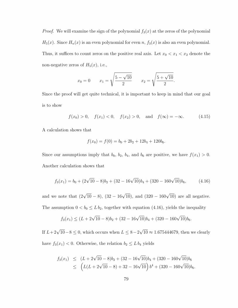
Proof. We will examine the sign of the polynomial f3(x) at the zeros of the polynomial

H5(x). Since Hn(x) is an even polynomial for even n, f3(x) is also an even polynomial.

Thus, it suffices to count zeros on the positive real axis. Let x0 < x1 < x2 denote the

non-negative zeros of H5(x), i.e.,

x0 = 0 x1 =

√5−

√10

2x2 =

√5 +

√10

2.

Since the proof will get quite technical, it is important to keep in mind that our goal

is to show

f(x0) > 0, f(x1) < 0, f(x2) > 0, and f(∞) = −∞. (4.15)

A calculation shows that

f(x0) = f(0) = b0 + 2b2 + 12b4 + 120b6.

Since our assumptions imply that b0, b2, b4, and b6 are positive, we have f(x1) > 0.

Another calculation shows that

f3(x1) = b0 + (2√

10− 8)b2 + (32− 16√

10)b4 + (320− 160√

10)b6, (4.16)

and we note that (2√

10 − 8), (32 − 16√

10), and (320 − 160√

10) are all negative.

The assumption 0 < b0 ≤ L b2, together with equation (4.16), yields the inequality

f3(x1) ≤ (L+ 2√

10− 8)b2 + (32− 16√

10)b4 + (320− 160√

10)b6.

If L+2√

10−8 ≤ 0, which occurs when L ≤ 8−2√

10 ≈ 1.675444679, then we clearly

have f3(x1) < 0. Otherwise, the relation b2 ≤ L b4 yields

f3(x1) ≤ (L+ 2√

10− 8)b2 + (32− 16√

10)b4 + (320− 160√

10)b6

≤(L(L+ 2

√10− 8) + 32− 16

√10)b4 + (320− 160

√10)b6.

79

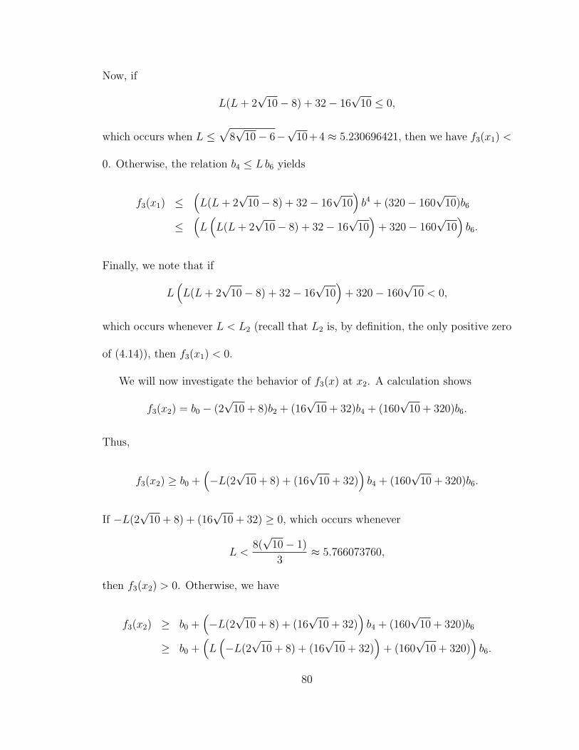
Now, if

L(L+ 2√

10− 8) + 32− 16√

10 ≤ 0,

which occurs when L ≤√

8√

10− 6−√

10+4 ≈ 5.230696421, then we have f3(x1) <

0. Otherwise, the relation b4 ≤ L b6 yields

f3(x1) ≤(L(L+ 2

√10− 8) + 32− 16

√10)b4 + (320− 160

√10)b6

≤(L(L(L+ 2

√10− 8) + 32− 16

√10)

+ 320− 160√

10)b6.

Finally, we note that if

L(L(L+ 2

√10− 8) + 32− 16

√10)

+ 320− 160√

10 < 0,

which occurs whenever L < L2 (recall that L2 is, by definition, the only positive zero

of (4.14)), then f3(x1) < 0.

We will now investigate the behavior of f3(x) at x2. A calculation shows

f3(x2) = b0 − (2√

10 + 8)b2 + (16√

10 + 32)b4 + (160√

10 + 320)b6.

Thus,

f3(x2) ≥ b0 +(−L(2

√10 + 8) + (16

√10 + 32)

)b4 + (160

√10 + 320)b6.

If −L(2√

10 + 8) + (16√

10 + 32) ≥ 0, which occurs whenever

L <8(√

10− 1)

3≈ 5.766073760,

then f3(x2) > 0. Otherwise, we have

f3(x2) ≥ b0 +(−L(2

√10 + 8) + (16

√10 + 32)

)b4 + (160

√10 + 320)b6

≥ b0 +(L(−L(2

√10 + 8) + (16

√10 + 32)

)+ (160

√10 + 320)

)b6.

80

Now, if

L(−L(2

√10 + 8) + (16

√10 + 32)

)+ (160

√10 + 320) ≥ 0,

which occurs whenever

L ≤ 88(√

10− 1)

3≈ 63.42681136,

then f3(x2) > 0. Finally we note that the leading coefficient of f3(x) is negative.

Therefore, f3(∞) = −∞.

We have now demonstrated that, for 0 < L < L2, the four inequalities (4.15)

hold and, therefore, f3(x) has at least 3 positive real zeros. Since f3(x) is an even

polynomial of degree 6, f3(x) has only real zeros.

The next lemma covers the remainder of the cases for our current goal.

Lemma 92. Let L1 denote the only positive zero of the polynomial

p(x) = x8 + 222!x6 + 244!x4 + 266!x2 − 287!

and suppose 0 < L ≤ L1 ≈ 4.462376406. If the sequence of positive real numbers

{b2k}∞k=0 satisfy the condition

0 < b0 < Lb2 < L2 b4 < L3b6 < · · ·

then, for any integer n ≥ 4,

n−1∑k=0

22k(2k)! b22k < 22n(2n− 1)! b22n. (4.17)

Proof. We first note that

p′(x) = 8x7 + 222!6x5 + 244!4x3 + 266!2x

81

has exactly one real zero, which is at the origin. Since p′(x) is a polynomial of odd

degree with positive leading coefficient, it follows that p′(x) is negative on the interval

(−∞, 0) and positive on the interval (0,∞). Since p(0) < 0, the assertion that p(x)

has exactly one positive zero is valid. Furthermore, p(x) ≤ 0 on the interval [0, L1],

from which we have the inequality

x8 + 222!x6 + 244!x4 + 266!x2 ≤ 287! (x ∈ [0, L1]).

We will prove the proposition by induction on n. First we consider the case when

n = 4. In this case, we have

3∑k=0

22k(2k)! b22k = b20 + 222!b22 + 244!b24 + 266!b26

< L8b28 + 222!L6b28 + 244!L4b28 + 266!L2b28=

(L8 + 222!L6 + 244!L4 + 266!L2

)b28

≤ 287!b28,

which is what was to be shown. Now suppose inequality (4.17) holds for some given

integer n ≥ 4. Then

n∑k=0

22k(2k)! b22k =n−1∑k=0

22k(2k)! b22k + 22n(2n)!b22n

< 22n(2n− 1)! b22n + 22n(2n)!b22n (4.18)

= 22n(2n− 1)! (1 + 2n) b22n.

Since we have assumed b2n < Lb2n+2, the inequality (4.18) becomes

n∑k=0

22k(2k)! b22k < 22n(2n− 1)! (2n+ 1)L2b22n+2

= 22n+2(2n+ 1)!b22n+2

L2

8n(4.19)

82

Noting that 8n ≥ 32, and L < 5, inequality (4.19) becomes

n∑k=0

22k(2k)! b22k < 22n+2(2n+ 1)!b22n+2,

as desired.

We can now give a slightly better lower bound for the value of L in Problem 85.

Proposition 93. Let L1 denote the only positive zero of the polynomial

p(x) = x8 + 222!x6 + 244!x4 + 266!x2 − 287!

(L1 ≈ 4.462376406) and suppose the sequence of positive real numbers {b2k}∞k=0 satisfy

the condition

0 < b0 ≤ L1 b2 ≤ L21 b4 ≤ L3

1b6 < · · · .

Then, for every non-negative integer n, the polynomial

n∑k=0

(−1)kb2kH2k(x)

has only real zeros.

Proof. By Lemma 87 the proposition holds for n = 0 and n = 1. By Lemmas 89 and

91, the proposition holds for n = 2 and n = 3. Finally, for n ≥ 4, the proposition

follows from Lemma 92 and Turan’s theorem regarding a sufficient condition for

the reality of zeros of a polynomial in terms of its Hermite expansion coefficients

(Theorem 84). We note that, although the inequality in Theorem 84 is strict, a

limiting argument shows that it is also valid when the inequality is non-strict.

83

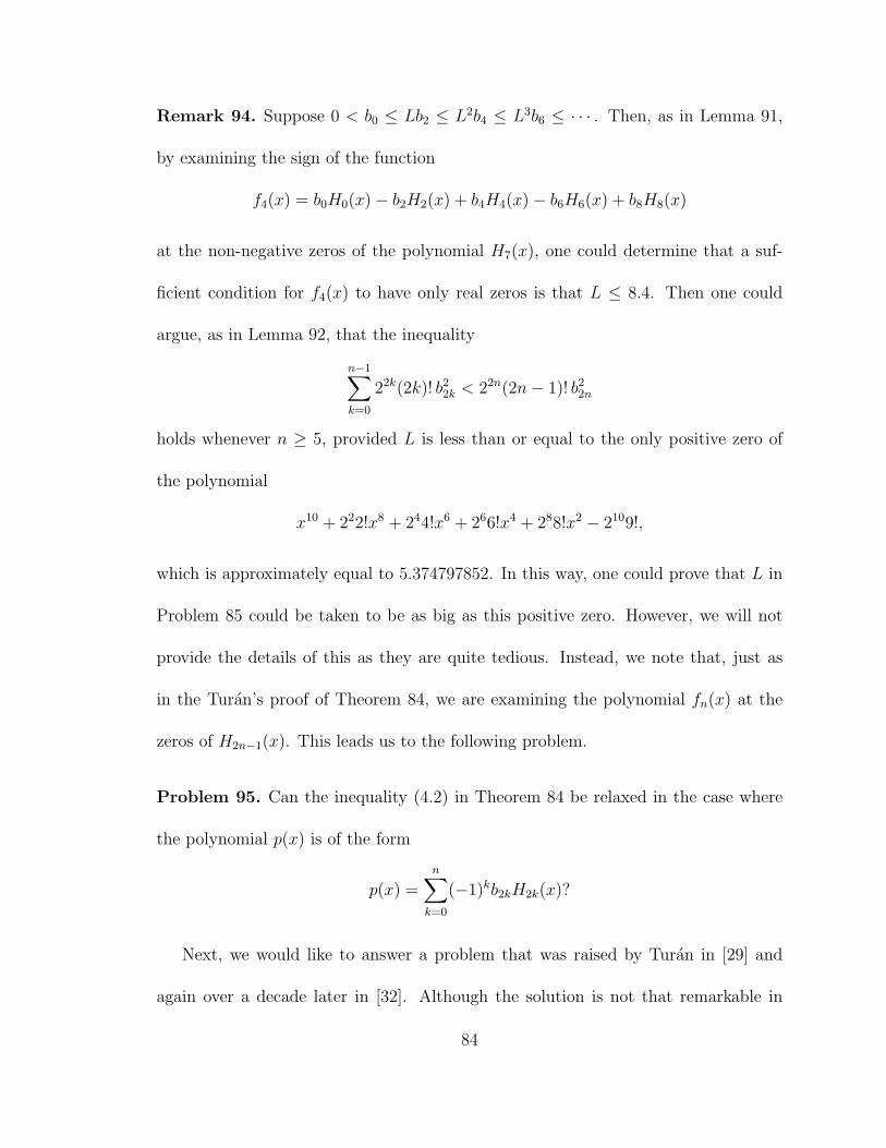
Remark 94. Suppose 0 < b0 ≤ Lb2 ≤ L2b4 ≤ L3b6 ≤ · · · . Then, as in Lemma 91,

by examining the sign of the function

f4(x) = b0H0(x)− b2H2(x) + b4H4(x)− b6H6(x) + b8H8(x)

at the non-negative zeros of the polynomial H7(x), one could determine that a suf-

ficient condition for f4(x) to have only real zeros is that L ≤ 8.4. Then one could

argue, as in Lemma 92, that the inequality

n−1∑k=0

22k(2k)! b22k < 22n(2n− 1)! b22n

holds whenever n ≥ 5, provided L is less than or equal to the only positive zero of

the polynomial

x10 + 222!x8 + 244!x6 + 266!x4 + 288!x2 − 2109!,

which is approximately equal to 5.374797852. In this way, one could prove that L in

Problem 85 could be taken to be as big as this positive zero. However, we will not

provide the details of this as they are quite tedious. Instead, we note that, just as

in the Turan’s proof of Theorem 84, we are examining the polynomial fn(x) at the

zeros of H2n−1(x). This leads us to the following problem.

Problem 95. Can the inequality (4.2) in Theorem 84 be relaxed in the case where

the polynomial p(x) is of the form

p(x) =n∑

k=0

(−1)kb2kH2k(x)?

Next, we would like to answer a problem that was raised by Turan in [29] and

again over a decade later in [32]. Although the solution is not that remarkable in

84

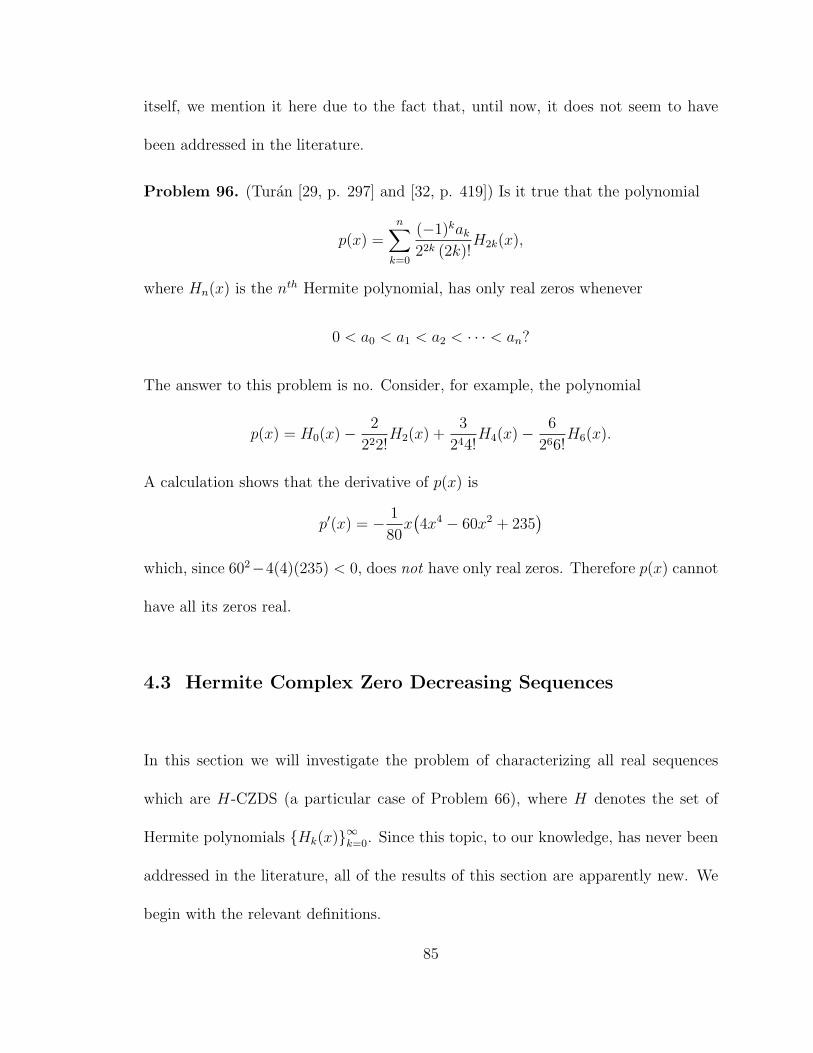
itself, we mention it here due to the fact that, until now, it does not seem to have

been addressed in the literature.

Problem 96. (Turan [29, p. 297] and [32, p. 419]) Is it true that the polynomial

p(x) =n∑

k=0

(−1)kak

22k (2k)!H2k(x),

where Hn(x) is the nth Hermite polynomial, has only real zeros whenever

0 < a0 < a1 < a2 < · · · < an?

The answer to this problem is no. Consider, for example, the polynomial

p(x) = H0(x)−2

222!H2(x) +

3

244!H4(x)−

6

266!H6(x).

A calculation shows that the derivative of p(x) is

p′(x) = − 1

80x(4x4 − 60x2 + 235

)which, since 602−4(4)(235) < 0, does not have only real zeros. Therefore p(x) cannot

have all its zeros real.

4.3 Hermite Complex Zero Decreasing Sequences

In this section we will investigate the problem of characterizing all real sequences

which are H-CZDS (a particular case of Problem 66), where H denotes the set of

Hermite polynomials {Hk(x)}∞k=0. Since this topic, to our knowledge, has never been

addressed in the literature, all of the results of this section are apparently new. We

begin with the relevant definitions.

85

Definition 97. Let {γk}∞k=0 be a sequence of real numbers. The TH-operator cor-

responding to the sequence {γk}∞k=0 is the linear operator on R[x] which is defined

by

TH [Hn(x)] = γnHn(x) (n = 0, 1, 2, . . . ).

Definition 98. A sequence of real numbers {γk}∞k=0 is called an Hermite Complex

Zero Decreasing Sequence or, for brevity, an H-CZDS (which we will also use in the

plural), if the TH-operator corresponding to the sequence {γk}∞k=0 has the property

that, for any real polynomial p(x),

ZC

(TH [p(x)]

)≤ ZC

(p(x)

),

where ZC(f(x)) is defined as in Notation 56.

Let us begin with the most elementary example of an H-CZDS.

Example 99. Any linear combination (over R) of consecutive Hermite polynomials

has only real zeros. Indeed, let α and β be any real numbers. Then, by the Hermite-

Poulain Theorem (Theorem 37), the relation H ′n(x) = 2nHn−1(x), and the fact that

Hn(x) has only real zeros,

αHn(x) + βHn−1(x) =

(α+

β

2nD

)[Hn(x)] ∈ L − P .

Therefore, any sequence of the form

{0, 0, 0, . . . , 0, γn, γn+1, 0, 0, 0, . . . } (γn, γn+1 ∈ R). (4.20)

is an H-CZDS.

Definition 100. We will call a sequence of the form (4.20) a trivial H-CZDS.

86

The existence of non-trivial H-CZDS is the consequence of the following gener-

alization of Turan’s theorem (Theorem 49), which can be thought of as a partial

analogue of Laguerre’s theorem (Theorem 60) for Hermite expansions.

Theorem 101. Suppose p(x) =n∑

k=0

akHk(x) is a real polynomial. If ϕ(x) ∈ L − P+,

then

ZC

(n∑

k=0

akϕ(k)Hk(x)

)≤ ZC

(n∑

k=0

akHk(x)

).

I.e., the sequence {ϕ(k)}∞k=0 is an H-CZDS.

Proof. We first consider the case ϕ(x) = α + x, where α ≥ 0. Let TH be the TH-

operator corresponding to the sequence {ϕ(k)}∞k=0 = {α+ k}∞k=0 and let

δ = xD − 1

2D2.

Then, from Hermite’s differential equation (2.7), we have

δHn(x) = nHn(x) (n = 0, 1, 2, . . . ).

Thus, for the real polynomial p(x) =n∑

k=0

akHk(x), we have

TH [p(x)] =n∑

k=0

ak(α+ k)Hk(x)

=n∑

k=0

ak(αI + δ)Hk(x)

= (αI + δ)n∑

k=0

akHk(x)

=

(αI + xD − 1

2D2

)p(x).

By Proposition 68 and our assumption α ≥ 0, the operator α + xD − 1/2D2 is a

complex zero decreasing operator. Therefore

87

ZC

(TH [p(x)]

)≤ ZC

(p(x)

).

Now suppose ϕ(x) ∈ L − P+ is a polynomial of degree m ≥ 2. Then ϕ(x) has

only real zeros and non-negative Taylor coefficients, i.e.,

ϕ(x) = c

m∏k=1

(x+ αk),

where c > 0 and αk ≥ 0. Therefore, the result follows from iteration of the previous

case.

Finally, suppose ϕ(x) is a transcendental entire function in the class L − P+.

Then there is a sequence of polynomials {ϕj(x)}∞j=0 ⊆ L− P+ which converge uni-

formly on compact subsets to ϕ(x). Let TjHdenote the TH-operator corresponding

to the sequence {ϕj(k)}∞k=0. Then, by the preceding results, the real polynomial p(x)

satisfies

ZC

(TjH

[p(x)])≤ ZC

(p(x)

)(j = 0, 1, 2, . . . ).

Since the sequence of polynomials {TjH[p(x)]}∞j=0 converge uniformly on compact

subsets to TH [p(x)], we have, by Hurwitz’ theorem, that

ZC

(TH [p(x)]

)≤ ZC

(p(x)

).

Remark 102. We stated that Theorem 101 is a partial analogue of Laguerre’s the-

orem (Theorem 60). As the following example shows, we cannot extend Laguerre’s

theorem in its full generality to Hermite expansions.

88

Example 103. The sequence {1/k!}∞k=0 is, by Laguerre’s theorem, a CZDS (see

Example 61). However, this sequence is not an H-CZDS. Indeed, if we let TH denote

the TH-operator associated with the sequence {1/k!}∞k=0, then

p(x) =1

2H0(x) +

1

4H2(x) =

1

2(1) +

1

4(4x2 − 2) = x2

does not have any non-real zeros, while

TH [p(x)] =1

2· 1

0!H0(x) +

1

4· 1

2!H2(x) =

1

2(1) +

1

8(4x2 − 2) =

1

2x2 +

1

4

has two non-real zeros.

The next result is the Hermite expansion analogue of a proposition due to Craven

and Csordas [11, Proposition 2.2].

Theorem 104. For every positive integer m the sequence

{k(k − 1)(k − 2) · · · (k −m+ 1)

p∏i=1

(k − bi)

}∞k=0

(bi ≤ m; i = 1, 2, 3, . . . , p)

(4.21)

is an H-CZDS.

Proof. Let TH be the TH-operator associated with the sequence (4.21) and let

δ = xD − 1

2D2.

Again, we note that, by Hermite’s Differential Equation (2.7),

δ[Hn(x)] = nHn(x) (n = 0, 1, 2, . . . ).

Thus, for any real polynomial p(x),

89

TH [p(x)] = δ(δ − 1)(δ − 2) · · ·(δ − (m− 1)

) p∏i=1

(δ − bi)[p(x)],

and, by Lemma 27,

TH [p(x)] =

(x− 1

2D

)m(

p∏i=1

((m− bi) + xD − 1

2D2

))Dm[p(x)].

By Rolle’s theorem, Dm is a complex zero decreasing operator. Similarly, for each i,

the assumption bi ≤ m implies m− bi ≥ 0. Thus the operator (m− bi +xD−1/2D2)

is, by Proposition 68, a complex zero decreasing operator. Finally, the operator

(x− 1/2D) is, by Proposition 67, a complex zero decreasing operator. Therefore,

ZC

(TH [p(x)]

)≤ ZC

(p(x)

).

Remark 105. Just as in Example 62, it can be shown that, for any m ≥ 2, the

sequence (4.21) cannot be interpolated by a function in L − P+. Indeed, if there

were such a function ϕ(x) =∞∑

k=0

αkxk ∈ L − P+ then the fact that ϕ(1) = 0 forces

all of the Taylor coefficients αk to be zero, contradicting the fact that ϕ(m+ 1) 6= 0.

Let us combine the preceding results into the following theorem which gives the

form of the most general H-CZDS known up to this point.

Theorem 106. For any function ϕ(x) ∈ L − P+ and any non-negative integer m,

the sequence

{ϕ(k)

(k(k − 1) · · · (k −m+ 1)

p∏i=1

(k − bi)

)}∞k=0

(bi ≤ m; i = 1, 2, 3, . . . , p)

(4.22)

90

is an Hermite complex zero decreasing sequence.

Proof. The result is an immediate consequence of Theorem 101, Theorem 104, and the

fact that the Hadamard product of two H-CZDS is again an H-CZDS. I.e., if {γk}∞k=0

and {λk}∞k=0 are two H-CZDS, then the sequence {γk · λk}∞k=0 is also an H-CZDS.

Indeed, given any real polynomial p(x) =n∑

k=0

akHk(x), we have

ZC

(n∑

k=0

akHk(x)

)≤ ZC

(n∑

k=0

akγkHk(x)

)≤ ZC

(n∑

k=0

akγkλkHk(x)

).

Example 103 showed that there are CZDS which are not H-CZDS. However, each

H-CZDS we have discovered thus far is a CZDS. We will prove that this is true in

general. To do so, we will need two technical lemmas which, together, give credence

to another Heuristic principle related to the operator exp(−D2/4). We have seen that

the operator exp(−D2/4) tends to attract the non-real zeros of a polynomial p(x) to

the real axis (Theorem 78) and that the following inequality always holds (Theorem

38).

ZC

(exp(−D2/4)[p(x)]

)≤ ZC(p(x)). (4.23)

However, if the imaginary parts of the non-real zeros of the given polynomial p(x)

are sufficiently large (how large generally depends on the degree of p(x)), then the

number of non-real zeros will not decrease, but remain the same, i.e., we will have

equality in (4.23). The following two lemmas together demonstrate this principle by

showing that if one moves the non-real zeros of a polynomial away from the real axis

91

via the transformation x 7→ x/j (where j is sufficiently large), then application of the

operator exp(−D2/4) does not change the number of non-real zeros of the resulting

polynomial.

Lemma 107. Let p(x) =n∑

k=0

akxk be a real polynomial and, for any non-zero real

constant j, define

qj(x) = exp

(−D

2

4j2

)[p(x)]

(D =

d

dx

). (4.24)

Then

qj

(x

j

)=

n∑k=0

ak

(2j)kHk(x) = exp(−D2/4)

[p

(x

j

)] (D =

d

dx

). (4.25)

Proof. For the convenience of the reader, we will recall here the main tool, which is

Equation (3.15) of Example 30.

exp(−α

2D2)

[xn] =(α

2

)n/2

Hn

(x√2α

) (α 6= 0, D =

d

dx

). (4.26)

Examining the left hand side of (4.25), we have

qj

(x

j

)=

[exp

(−D

2

4j2

)[p(w)]

]w= x/j

(D =

d

dw

)which, by (4.26), becomes

qj

(x

j

)=

[n∑

k=0

ak

(1

2j

)k

Hk (jw)

]w= x/j

=n∑

k=0

ak

(1

2j

)k

Hk(x).

Similarly, examining the right hand side of (4.25), we have

exp

(−D

2

4

)[p

(x

j

)]= exp

(−D

2

4

)[ n∑k=0

ak

(x

j

)k] (

D =d

dx

)

92

which, by (4.26), becomes

exp

(−D

2

4

)[p

(x

j

)]=

n∑k=0

ak

(1

2j

)k

Hk(x)

(D =

d

dx

).

Thus, equation (4.25) holds as claimed.

We will now take j to be any non-zero natural number in Lemma 107 to obtain a

sequence of functions which have a desirable property.

Lemma 108. Let p(x) =n∑

k=0

akxk be a real polynomial and define

qj(x) = exp

(−D

2

4j2

)[p(x)]

(D =

d

dx; j = 1, 2, 3, . . .

).

Then there exists a natural number N such that

ZC

(qj

(x

j

))= ZC

(p(x)

)whenever j ≥ N .

Proof. By Lemma 107 and the fact that the operator exp(−D2/4) is a complex zero

decreasing operator (see Theorem 38),

ZC

(qj

(x

j

))= ZC

(exp

(−D

2

4

)[p

(x

j

)])≤ ZC

(p

(x

j

))= ZC

(p(x)

). (4.27)

Since the coefficients of

qj(x) = exp

(−D

2

4j2

)[p(x)] =

[n/2]∑k=0

(− 1

4j2

)k1

k!p(2k)(x)

tend to the coefficients of p(x) as j → ∞, the polynomials {qj(x)}∞j=1 converge uni-

formly on compact subsets of C to p(x). Therefore, by Hurwitz’ theorem, there exists

an integer N such that

93

ZC

(p(x)

)≤ ZC

(qj(x)

)= ZC

(qj

(x

j

))whenever j ≥ N . Comparing with (4.27) yields the result.

We are now in a position to prove that every Hermite complex zero decreasing

sequence is a classical complex zero decreasing sequence.

Proposition 109. If the sequence {γk} is an H-CZDS, then {γk}∞k=0 is a CZDS.

Proof. By way of contradiction, suppose the sequence {γk}∞k=0 is an H-CZDS which

is not a classical CZDS. Then there exists a polynomial f(x) =n∑

k=0

akxk which has

the property that

ZC

(p(x)

)> ZC

(f(x)

), (4.28)

where p(x) =n∑

k=0

akγkxk. By Lemma 108, there exists an integer N such that

ZC

(qN

( xN

))= ZC

(p(x)

), (4.29)

where

qN(x) = exp

(− D2

4N2

)[p(x)] .

Since the operator exp(−D2/4) is a complex zero decreasing operator,

ZC

(f(x)

)= ZC

(f( xN

))≥ ZC

(exp(−D2/4)

[f( xN

)]). (4.30)

By equation (4.25) of Lemma 107 and our assumption that {γk}∞k=0 is an H-CZDS,

ZC

(exp(−D2/4)

[f( xN

)])= ZC

(n∑

k=0

ak

(2N)kHk(x)

)

≥ ZC

(n∑

k=0

ak

(2N)kγkHk(x)

)(4.31)

= ZC

(qN

( xN

)).

94

Thus, by (4.29), (4.30), and (4.31) we have ZC

(f(x)

)≥ ZC

(p(x)

), which contradicts

(4.28).

Remark 110. Before the end of this dissertation, we shall come across another proof

of Proposition 109 which does not require the use of the operator exp(−D2/4). This

method will then be used to show that, remarkably, every Q-CZDS must be a CZDS,

regardless of the choice of the basis Q. However, we shall postpone this discussion

until we arrive at a more suitable setting.

With the aid of Proposition 109, we may now prove the Hermite expansion ana-

logue of the characterization of H-CZDS which can be interpolated by a polynomial

(Theorem 63).

Theorem 111. Let h(x) be a real polynomial. Then {h(k)}∞k=0 is an H-CZDS if and

only if either

1. h(0) 6= 0 and h(x) has only real negative zeros, or

2. h(0) = 0 and h(x) is of the form

h(x) = x(x− 1)(x− 2) · · · (x−m+ 1)

p∏k=1

(x− bk) (4.32)

where m ≥ 1 and p ≥ 0 are integers and bk < m for k = 1, 2, 3, . . . , p.

Proof. Suppose {h(k)}∞k=0 is an H-CZDS. Then, by Proposition 109, {h(k)}∞k=0 is a

CZDS and the result is an immediate consequence of Theorem 63.

95

Conversely, if h(x) has only real negative zeros, then, by Theorem 101, {h(k)}∞k=0

is an H-CZDS. If h(x) is of the form (4.32), then, by Theorem 104, {h(k)}∞k=0 is an

H-CZDS.

4.4 Hermite Multiplier Sequences

In this section we will return to the problem of finding an Hermite expansion analogue

of Polya and Schur’s characterization of multiplier sequences (see Problem 50). In

analogy to the concept of a multiplier sequence, we make the following definition.

Definition 112. A sequence of real numbers {γk}∞k=0 is called an Hermite multiplier

sequence or, for brevity, an H-multiplier sequence if it has the property that its

corresponding TH-operator preserves reality of zeros. I.e., the sequence {γk}∞k=0 has

the property that

n∑k=0

akγkHk(x) ∈ L − P whenevern∑

k=0

akHk(x) ∈ L − P (ak ∈ R).

By Turan’s theorem (Theorem 49), any sequence which can be interpolated by a real

polynomial having only real zeros is an H-multiplier sequence. Furthermore, the gen-

eralization of Bleecker and Csordas [1, Theorem 2.7] states that any sequence which

can be interpolated by a function in the class L − P+ is an H-multiplier sequence.

As far as we know, these (i.e., sequences which can be interpolated by functions in

L − P+) are the only H-multiplier sequences which have been previously discovered.

96

That we have already discovered some new H-multiplier sequences is a conse-

quence of the results of the previous section and the following lemma.

Lemma 113. If {γk}∞k=0 is an H-CZDS, then {γk}∞k=0 is an H-multiplier sequence.

Proof. We first note that a real polynomial q(x) belongs to the class L − P if and only

if ZC

(q(x)

)= 0. Let TH be the TH-operator associated with the H-CZDS {γk}∞k=0.

If p(x) is a real polynomial which belongs to the class L − P , then

ZC

(TH [p(x)]

)≤ ZC

(p(x)

)= 0,

Thus ZC

(T [p(x)]

)= 0, which implies T [p(x)] ∈ L − P . Therefore {γk}∞k=0 is an

H-multiplier sequence.

Example 114. By Example 99, any sequence of the form

{0, 0, 0, . . . , 0, γn, γn+1, 0, 0, 0, . . . } (γn, γn+1 ∈ R). (4.33)

is an H-CZDS and, therefore, is also an H-multiplier sequence.

Definition 115. We will call a sequence of the form (4.33) a trivial H-multiplier

sequence.

Proposition 116. For any function ϕ(x) ∈ L − P+ and any non-negative integer

m, the sequence

{ϕ(k)

(k(k − 1) · · · (k −m+ 1)

p∏i=1

(k − bi)

)}∞k=0

(bi ≤ m; i = 1, 2, 3, . . . , p)

(4.34)

is an Hermite multiplier sequence.

97

Proof. The sequence (4.34) is, by Theorem 106 an H-CZDS. Therefore, by Lemma

113, it is also an H-multiplier sequence.

Remark 117. Since, for m ≥ 2, it is easy to see that the sequences of the form

(4.34) cannot be interpolated by any function in the class L − P+ (see Remark 105),

these Hermite multiplier sequences are indeed different from those which were already

known.

By Proposition 109, every H-CZDS is also a CZDS. As it turns out, we can adapt

this result to our current setting.

Proposition 118. If {γk}∞k=0 is an H-multiplier sequence, then it is a (classical)

multiplier sequence.

Proof. The proof is the same as that of Proposition 109, except we choose the poly-

nomial f(x) so that, in equation (4.28), we have ZC

(f(x)

)= 0 .

By Proposition 118, most of the properties of multiplier sequences given in Propo-

sition 45 carry over to H-multiplier sequences. However, we will see that the converse

of Proposition 118 is false, i.e., there are classical multiplier sequences which are

not H-multiplier sequences. Therefore, some justification is required for some of the

following assertions.

Proposition 119. Let {γk}∞k=0 be an H-multiplier sequence. Then

(1) If there exists an integer m ≥ 0 such that γm 6= 0 and an integer n > m such

that γn = 0, then γk = 0 for all k ≥ n.

98

(2) The elements of {γk}∞k=0 are either all of the same sign, or they alternate in

sign.

(3) The sequence{(−1)kγk

}∞k=0

is also an H-multiplier sequence.

(4) For any r ∈ R, the sequence {rγk}∞k=0 is also an H-multiplier sequence.

(5) The elements of {γk}∞k=0 satisfy Turan’s inequality

γ2k − γk−1γk+1 ≥ 0 (k = 1, 2, 3, . . . ). (4.35)

Proof. By Proposition 118, the H-multiplier sequence {γk}∞k=0 is also a multiplier

sequence. Therefore, properties (1), (2), and (5) follow from Proposition 45.

Property (3) follows from the relation Hn(−x) = (−1)nHn(x). Indeed, if

p(x) =n∑

k=0

akHk(x)

is a real polynomial with only real zeros, then

f(x) = TH [p(x)] =n∑

k=0

akγkHk(x) ∈ L − P ,

where TH is the TH-operator associated with the sequence {γk}∞k=0. Therefore,

f(−x) =n∑

k=0

akγkHk(−x) =n∑

k=0

ak(−1)kγkHk(x) ∈ L − P .

Property (4) is trivial. Indeed, if

p(x) =n∑

k=0

akHk(x)

is a real polynomial with only real zeros, then

n∑k=0

akrγkHk(x) = rn∑

k=0

akγkHk(x) = rTH [p(x)] ∈ L − P .

99

Remark 120. Suppose {γk}∞k=0 is an H-multiplier sequence. Then, by proper-

ties (3) and (4) of Proposition 119, the sequences {−γk}∞k=0,{(−1)kγk

}∞k=0

, and{(−1)k+1γk

}∞k=0

are also H-multiplier sequences. Furthermore, by property (2) of

Proposition 119, one of these sequences consists entirely of non-negative elements.

In what follows, we will often restrict our attention to non-negative H-multiplier

sequences. One should keep in mind that analogous results hold in the general case.

In the previous section, we saw that the sequence {1/k!}∞k=0 is not an H-CZDS (see

Example 103). The same example used to show this can be used to see that {1/k!}∞k=0

is not an H-multiplier sequence either. The goal of the remainder of this section is

to show that, in general, any non-trivial H-multiplier sequence whose elements are

non-negative must be non-decreasing. First, we will demonstrate several preparatory

results which are of interest in their own right.

Lemma 121. Let n ≥ 4 be an integer and suppose x1and x2 are consecutive zeros of

Hn(x) of the same sign. Then Hn−2(x1)Hn−2(x2) < 0.

Proof. From the pure recurrence relation(see equation (2.6)

)Hn(x) = 2xHn−1(x)− 2(n− 1)Hn−2(x)

and the fact that x1 and x2 are zeros of Hn(x), we have the two equations

0 = Hn(x1) = 2x1Hn−1(x1)− 2(n− 1)Hn−2(x1)

0 = Hn(x2) = 2x2Hn−1(x2)− 2(n− 1)Hn−2(x2).

Thus

100

Hn−2(x1)Hn−2(x2) =x1

n− 1Hn−1(x1)

x2

n− 1Hn−1(x2). (4.36)

By the relation(see equation (2.5)

)H ′

n(x) = 2nHn−1(x),

equation (4.36) becomes

Hn−2(x1)Hn−2(x2) =x1x2

4n2(n− 1)2H ′

n(x1)H′n(x2). (4.37)

Furthermore, since the zeros of Hn(x) are all simple and x1 and x2 are consecu-

tive zeros of Hn(x), we have H ′n(x1)H

′n(x2) < 0. This fact, together with equation

(4.37) and the fact that we have chosen x1 and x2 to be the same sign, shows that

Hn−2(x1)Hn−2(x2) < 0.

Remark 122. In particular, Lemma 121 implies that there is a zero of Hn−2(x)

between every pair of consecutive zeros of Hn(x). In light of the fact that Hn−2(x)

is a scalar multiple of the second derivative of Hn(x), this is somewhat remarkable.

In general, the zeros of the second derivative of a polynomial are not always so well

behaved. Consider, for example, the (even) polynomial

q(x) = (x2 − 1)(x2 − 4) = x4 − 5x2 + 4.

The second derivative of q(x) is q′′(x) = 2(6x2 − 5) which does not have any zeros in

the interval (1, 2).

The next two technical lemmas will also be needed in what follows.

101

Lemma 123. Let a > 0 and suppose the function f(x) is differentiable on the interval

[0, a]. If f(x) has a simple zero at x = 0, is non-zero at x = a, and has exactly m

zeros (counting multiplicities) in the interval (0, a), then (−1)mf ′(0)f(a) > 0.

Proof. Let x0 denote the smallest zero of f(x) in the interval (0, a) (if f(x) has no

zeros in this interval, set x0 = a). Then

(−1)mf(x)f(a) > 0 for all x ∈ (0, x0).

Therefore, by the definition of the derivative and the fact that f(0) = 0,

(−1)mf ′(0)f(a) = (−1)m limx→0+

f(x)− f(0)

x− 0f(a) = lim

x→0+

(−1)mf(x)f(a)

x≥ 0.

By assumption, f ′(0)f(a) 6= 0, thus (−1)mf ′(0)f(a) > 0.

Lemma 124. Let n ≥ 3 be an odd natural number and let a denote the smallest

positive zero of Hn(x). Then Hn(x) has constant sign on the interval (0, a) and, for

any x0 ∈ (0, a),

sign(Hn(x0)

)= sign

(Hn−1(0)

).

Proof. Since n is odd, Hn(0) = 0. Since the zeros of Hn−1(x) are all simple and

separated by the zeros of Hn(x), we have

Hn−1(0)Hn−1(a) < 0. (4.38)

From the relation(see (2.5)

)H ′

n(x) = 2nHn−1(x)

we have

102

Hn−1(a) =1

2nH ′

n(a) =1

2nlimx→a

Hn(x)−Hn(a)

x− a=

1

2nlim

x→a−

Hn(x)

x− a.

Therefore, the sign of Hn−1(a) is opposite of the sign of Hn(x) on the interval (0, a).

By inequality (4.38), the sign of Hn−1(0) is the same as the sign of Hn(x) on the

interval (0, a), which is what was to be shown.

Proposition 125. Let n ≥ 2 be an integer and suppose β ∈ R. Then the polynomial

fn,β(x) = Hn(x) + βHn−2(x)

has only real zeros if and only if β ≤ 4[

n+12

]− 2.

Proof. Let us first consider the cases n = 2 and n = 3. From the equation

f2,β(x) = H2(x) + βH0(x) = 4x2 − 2 + β,

we see that f2,β(x) has only real zeros if and only if β ≤ 2 = 4[

2+12

]− 2. Similarly,

from the equation

f3,β(x) = H3(x) + βH1(x) = 8x3 + (2β − 12)x,

we see that f3,β(x) has only real zeros if and only if β ≤ 6 = 4[

3+12

]− 2.

Now suppose n ≥ 4 and β ≤ 0. In this case, the polynomial

2nxn + β2n−2xn−2 = (2x)n−2(4x2 − β)

has only real zeros. Thus, since the operator exp(−D2/4) preserves reality of zeros,

exp(−D2/4)[2nxn + β2n−2xn−2

]= Hn(x) + βHn−2(x) = fn,β(x)

has only real zeros.

Finally we consider the case where n ≥ 4 and β > 0. Since the Hermite polyno-

mials satisfy the relation Hk(−x) = (−1)kHk(x), we have

103

fn,β(−x) = (−1)nfn,β(x). (4.39)

In light of this fact, we will count the number of zeros of fn,β(x) on the positive real

axis. Let

0 < x1 < x2 < · · · < xm

(m =

[n2

])denote the positive zeros of Hn(x). By Lemma 121,

fn,β(xi)fn,β(xi+1) = β2Hn−2(xi)Hn−2(xi+1) < 0 (i = 1, 2, 3, . . . ,m− 1).

Therefore, for each i = 1, 2, 3, . . . ,m−1, the polynomial fn,β(x) has an odd number of

zeros in the interval (xi, xi+1). We claim that fn,β(x) has exactly one zero (counting

multiplicities) in each of these intervals. Indeed, if this were not the case, then fn,β(x)

would have at least (m − 1) + 2 = m + 1 positive zeros. By equation (4.39), fn,β(x)

would then have at least 2m+ 2 real zeros. But

2m+ 2 = 2[n2

]+ 2 ≥ n+ 1

and, since deg(fn,β(x)

)= n, we have contradicted the Fundamental Theorem of

Algebra. Therefore, fn,β(x) has exactly one zero in each of the intervals (xi, xi+1) as

claimed. Furthermore, we have now demonstrated that fn,β(x) has at least

2m− 2 = 2[n2

]− 2 =

{n− 2 if n is evenn− 3 if n is odd

(4.40)

real zeros, each of which lies in (−xm,−x1) ∪ (x1, xm).

We claim that fn,β(x) does not have any zeros in the interval (xm,∞). Indeed,

Hn(x) and Hn−2(x) are both positive on the interval (xm,∞) and we have assumed

104

β > 0. Whence, fn,β(x) is also positive and, therefore, does not vanish on the interval

(xm,∞). Similarly, fn,β(x) does not have any zeros in the interval (−∞,−xm).

The question of whether or not fn,β(x) has only real zeros now depends entirely

on its behavior in the interval (−x1, x1). From the explicit formula for the Hermite

polynomials (2.3), we have

Hk(0) =

(−1)k/2k!

(k/2)!if k is even

0 if k is odd

(4.41)

In particular, if k ≥ 2 is even, then a calculation shows that

Hk(0) = −2(k − 1)Hk−2(0). (4.42)

Suppose n is even. In this case we only have two zeros to account for (see equation(4.40)

). Thus fn,β(x) has only real zeros if and only if it has a zero in the interval

[0, x1), which occurs if and only if f(0)f(x1) ≤ 0. By equation (4.42) and the fact

that Hn(x1) = 0,

f(0)f(x1) =(Hn(0) + βHn−2(0)

)(Hn−2(x1)

)=(− 2(n− 1) + β

)Hn−2(0)Hn−2(x1).

Since Hn−2 does not vanish on [−x1, x1], we see that fn,β(0)fn,β(x1) ≤ 0 if and only

if −2(n− 1) + β ≤ 0. Therefore, fn,β(x) has only real zeros if and only if

β ≤ 2(n− 1) = 2n− 2 = 4

[n+ 1

2

]− 2.

Now suppose n is odd. In this case fn,β(x) will have only real zeros if and only if

fn,β(x) either has a multiple zero at the origin, or has a simple zero at the origin and

another simple zero in the interval (0, x1). In the former case, f ′(0) = 0 and in the

105

latter, by Lemma 123, f ′(0)f(x1) < 0. Thus fn,β(x) has only real zeros if and only if

f ′(0)f(x1) ≤ 0. But

f ′(0)f(x1) =[H ′

n(0) + βH ′n−2(0)

]Hn−2(x1)

=[2nHn−1(0) + β2(n− 2)Hn−3(0)

]Hn−2(x1),

which, by equation (4.42), becomes

f ′(0)f(x1) = 2(n− 2)(β − 2n)Hn−3(0)Hn−2(x1).

Since x1 lies in the interval (0, a), where a is the smallest positive zero of Hn−2(x),

we have by, Lemma 124, that Hn−3(0)Hn−2(x1) > 0. Therefore f ′(0)f(x1) ≤ 0 if and

only if β − 2n ≤ 0. I.e. fn,β(x) has only real zeros if and only if

β ≤ 2n = 2(n+ 1)− 2 = 4

[n+ 1

2

]− 2.

The usefulness of Proposition 125 lies in the fact that it gives a necessary and

sufficient condition for reality of zeros of a particular type of Hermite expansion.

Lemma 126. If the sequence of non-negative real numbers {γk}∞k=0 is a non-trivial

H-multiplier sequence, then there exists an integer m ≥ 0 such that γk = 0 for every

non-negative integer k < m and γk 6= 0 for every integer k ≥ m.

Proof. Since {γk}∞k=0 is a non-trivial H-multiplier sequence, it has at least one non-

zero element (see Definition 115). Set m = min{k : γk 6= 0}. We claim that γm+1 and

γm+2 are non-zero. Indeed, if either of them were zero, then, by property (1) of Propo-

sition 119, all subsequent elements of the sequence would also be zero, contradicting

the fact that the sequence is a non-trivial H-multiplier sequence.

106

By way of contradiction, suppose there is an integer n > m+ 2 for which γn = 0.

By Proposition 125, we can choose am and am+2 so that the polynomial

p(x) = amγmHm(x) + am+2γm+2Hm+2(x) 6∈ L − P .

By the theorem of Turan which gives a sufficient condition for reality of zeros of an

Hermite expansion (Theorem 84), we may pick an large enough so that

f(x) = amHm(x) + am+2Hm+2(x) + anHn(x) ∈ L − P .

But then TH [f(x)] = p(x) 6∈ L − P , where TH denotes the TH-operator corresponding

to the sequence {γk}∞k=0. Thus we have contradicted the fact that {γk}∞k=0 is an H-

multiplier sequence. Therefore, ak 6= 0 for all k ≥ m.

Theorem 127. If the sequence of non-negative real numbers {γk}∞k=0 is a non-trivial

H-multiplier sequence, then γk ≤ γk+1 for every integer k ≥ 0.

Proof. By Lemma 126, there exists an integer m ≥ 0 such that γk = 0 for k < m and

γk 6= 0 for k ≥ m. Fix an integer n such that n ≥ m. Note that, in particular, γn,

γn+1, and γn+2 are each non-zero. By Lemma 125, the polynomial

f(x) = Hn+2(x) +

(4

[n+ 3

2

]− 2

)Hn(x)

has only real zeros. Let TH denote the TH-operator associated with the H-multiplier

sequence {γk}∞k=0. Then

TH [f(x)] = γn+2

(Hn+2(x) +

(4

[n+ 3

2

]− 2

)γn

γn+2

Hn(x)

)has only real zeros. Thus, by Lemma 125,(

4

[n+ 3

2

]− 2

)γn

γn+2

≤(

4

[n+ 3

2

]− 2

). (4.43)

107

Since(4[

n+22

]− 2)> 0, it follows from (4.43) and the fact that γn 6= 0 that

0 <γn

γn+2

≤ 1. (4.44)

By Property 5 of Proposition 119, every H-multiplier sequence satisfies Turan’s in-

equality (4.35). Thus,

γ2n+1 − γnγn+2 ≥ 0,

from which we have (γn+1

γn

)2

− γn+2

γn

≥ 0. (4.45)

Thus, by the inequalities (4.44) and (4.45),(γn+1

γn

)2

≥ γn+2

γn

≥ 1.

Therefore γn ≤ γn+1.

Remark 128. Any sequence which is not an H-multiplier sequence cannot be an H-

CZDS (see Lemma 113). Thus, any H-CZDS which consists entirely of non-negative

elements must be non-decreasing.

Corollary 129. For any r > 0, the sequence{rk}∞

k=0is an H-CZDS if and only if

r ≥ 1.

Proof. If 0 < r < 1, then{rk}∞

k=0is a sequence of decreasing non-negative numbers.

Therefore, by Theorem 127 and Remark 128,{rk}∞

k=0is not an H-CZDS.

If r ≥ 1, then the sequence{rk}∞

k=0can be interpolated by the function

rx = exp(ln rx) = exp(x ln r)

108

which, since ln r ≥ 0, belongs to the class L − P+. Therefore, by Proposition 101,{rk}∞

k=0is an H-CZDS.

So far, everyH-multiplier sequence which we have come across is also anH-CZDS.

One may be inclined to ask if there are any H-multiplier sequences which are not H-

CZDS. Indeed, in the classical setting we have seen that there are multiplier sequences

which are not CZDS (see Example 64). In particular, one could ask whether or not

the multiplier sequence{1 + k + k2

}∞k=0

(which is not a CZDS and, therefore, not

an H-CZDS) is an H-multiplier sequence. However, none of the methods we have

developed thus far yield an answer to this question. In the next chapter, we will see

that{1 + k + k2

}∞k=0

is an H-multiplier sequence. In order to prove this, we shall

generalize a curve theorem due to Polya, which itself is a sort of unification of three

major results in this area which we have already seen.

Before moving on to the discussion of the curve theorem, we will demonstrate

why one is inclined to believe that every non-negative multiplier sequence which is

non-decreasing must also be an H-multiplier sequence. As it turns out, non-negative

multiplier sequences which are non-decreasing enjoy a remarkable geometric property.

Theorem 130. (Gauss-Lucas Theorem [33, p. 84]) Let K be any convex polygon

enclosing all the zeros of the polynomial f(z). Then the zeros of f ′(z) lie in K.

Craven and Csordas examined the Gauss-Lucas Theorem in the context of multiplier

sequences, which led them to make the following definition.

109

Definition 131. ([8, p. 419]) A sequence {γk}∞k=0 of real numbers is said to possess

the Gauss-Lucas property if it satisfies the following condition. Let f(z) =n∑

k=0

akzk

be an arbitrary complex polynomial. If K is a convex region containing the origin

and all the zeros of f(z), and if the polynomial g(z) =n∑

k=0

akγkzk is not identically

zero, then the zeros of g(z) also lie in K.

If the polynomial f(z) in Definition 131 has only real zeros, then we may take K

to be a closed interval of real numbers, and we see that the resulting polynomial g(z)

will also have only real zeros. Thus, every sequence which possesses the Gauss-Lucas

property is also a multiplier sequence. Furthermore, by the Gauss-Lucas Theorem,

the sequence {k}∞k=0 possesses the Gauss-Lucas property. Craven and Csordas showed

that this is true of any non-negative multiplier sequence which is non-decreasing, and,

in fact, these are the only sequences which posses the Gauss-Lucas property.

Theorem 132. (Craven-Csordas [8, Theorem 2.8]) The sequence of non-negative

real numbers {γk}∞k=0 possesses the Gauss-Lucas property if and only if {γk}∞k=0 is a

multiplier sequence which satisfies 0 ≤ γn ≤ γn+1 for all non-negative integers n.

The next lemma will allow us to relate these results to H-multiplier sequences.

Lemma 133. Let {γk}∞k=0 be a sequence of real numbers and define the linear oper-

ators T and TH on R[x] by

T [xn] = γnxn (n = 0, 1, 2, . . . ) (4.46)

andTH [Hn(x)] = γnHn(x) (n = 0, 1, 2, . . . ),

110

where Hn(x) denotes the nth Hermite polynomial. Then, for any polynomial p(x),

TH [p(x)] =(e−

D2

4 T eD2

4

)[p(x)].

Proof. By relation (3.15), we have

e−D2

4 [xn] =1

2nHn(x) (n = 0, 1, 2, . . . ),

from which we also obtain

eD2

4 [Hn(x)] = (2x)n (n = 0, 1, 2, . . . ). (4.47)

Thus, for any n = 0, 1, 2, . . . , we have

(e−

D2

4 T eD2

4

)[Hn(x)] =

(e−

D2

4 T)

[2nxn]

=(e−

D2

4

)[2nγnx

n]

= γnHn(x).

Therefore the linear operators TH and e−D2

4 T eD2

4 , since they agree on the basis

elements Hn(x) (n = 0, 1, 2, . . . ), are equal on all of R[x].

Remark 134. Suppose {γk}∞k=0 is a non-negative multiplier sequence which is non-

decreasing. Then the following heuristic principle leads us to believe that the sequence

{γk}∞k=0 must also be an H-multiplier sequence. If the zeros of p(x) are all real, then

the polynomial f(x) = eD2

4 [p(x)] will generally have non-real zeros. By Theorem 132,

the zeros of T [f(x)] will lie in the convex hull of the zeros of f(x), where T is defined

by (4.46). In particular the imaginary parts of the zeros of T [f(x)] will generally be

smaller than those of f(x). Thus the polynomial TH [p(x)] = e−D2

4 [T [f(x)]] should

have all its zeros real.

111

A more precise result is demonstrated by the following proposition.

Proposition 135. Let {γk}∞k=0 be a non-negative multiplier sequence which is non-

decreasing and let TH denote the TH-operator associated with the sequence {γk}∞k=0.

If p(x) is a real polynomial having only real zeros, and if f(x) = eD2

4 [p(x)] has all its

zeros in the strip S(√

2) ={z : Im z ≤

√2}, then the polynomial TH [p(x)] ∈ L − P.

Proof. Let T be the linear operator on R[x] defined by T [xn] = γnxn (n = 0, 1, 2, . . . ).

Then, by Theorem 132, either the polynomial T [f(x)] is identically zero or all of its

zeros lie in the strip S(√

2). Therefore, by Lemma 133 and Corollary 79,

TH [p(x)] =(e−

D2

4 T eD2

4

)[p(x)] = e−

D2

4

[T [f(x)]

]∈ L − P .

Unfortunately, if p(x) has only real zeros, then the zeros of eD2

4 [p(x)] need not lie

in the strip S(√

2). Indeed, by the relation (3.15),

eD2

4 [xn] =(−1)n

2nHn(−ix),

and the imaginary part of the zeros of Hn(−ix) become arbitrarily large as n→∞.

Therefore, we will need to develop other methods to show that every non-negative

multiplier sequence which is non-decreasing must also be an H-multiplier sequence.

112

Chapter 5

A Curve Theorem

5.1 Polya’s Curve Theorem

In 1916, Polya discovered a result which he stated as follows.

Theorem 136. (Polya [25]) Suppose the real polynomial

f(x) = a0 + a1x+ · · ·+ anxn (an 6= 0)

has only real zeros and that

q(x) = b0 + b1x+ · · ·+ bnxn + bn+1x

n+1 + · · ·+ bn+mxn+m (5.1)

(m ≥ 0) also has only real zeros and that the first n + 1 coefficients b0, b1, b2, . . . , bn

are all positive. Then the nth order curve

F (x, y) = b0f(y) + b1xf′(y) + b2x

2f ′′(y) + · · ·+ bnxnf (n)(y) = 0 (5.2)

has n intersection points with each of the lines

sx− ty + u = 0, (5.3)

where s ≥ 0, t ≥ 0, s+ t > 0, and u ∈ R.

Figure 1 below demonstrates the graphical representation of the curve F (x, y) = 0,

where we have chosen q(x) = (1 + x)4 and f(x) = x3 − x. In general, by declaring

that (5.2) is an nth order curve, it is meant that there are n curves in the plane such

that the set {(x, y) : F (x, y) = 0} is equal to the union of the images of these curves.

113

Figure 1: The curve F (x, y) = 0 for deg(q) > deg(f).

By declaring that a given line has n intersection points with the nth-order curve, it is

meant (in this particular setting) that the line intersects each of the n curves exactly

once. This clarification is important since, in general, the actual number of points of

intersection between the given line and the set {(x, y) : F (x, y) = 0} may be less than

n. Thus, we must bear in mind that we are counting intersections with some sort of

a notion multiplicity. Indeed, by solving for one of the variables x or y in terms of

the other in the equation of the line (5.3) and then substituting into the polynomial

F (x, y), we obtain a polynomial in one variable. Each real zero of the resulting

polynomial in one variable corresponds to an intersection point and, conversely, every

intersection point corresponds to a real zero of the resulting polynomial. Thus, the

intersection point which corresponds to a zero of multiplicity m should be considered

as an intersection point of multiplicity m. These clarifications bring to light the

true nature of this theorem. Although the theorem itself is geometric in nature, the

underlying theme is that of transformations which preserve reality of zeros.

114

We also note that, in a more general setting, if G(x, y) is an arbitrary polynomial

in two variables x and y and G(x, y) = 0 represents an nth order curve, then it is

possible that a given line does not have any intersections with one of the n curves.

Similarly, it is possible that a given line has several intersections with only one of the

n curves.

In the original proof of Theorem 136, Polya omitted several technical details which

demonstrate that these curves do indeed exist. The goal of this chapter is to justify

the existence of these curves and to prove another curve theorem which is better suited

to polynomials of arbitrary degree. Before getting into this detailed discussion, let us

get a better feel for Theorem 136 by examining several important special cases.

In the case where x = 1, equation (5.2) reduces to

b0f(y) + b1f′(y) + b2f

′′(y) + · · · bnf (n)(y) = 0.

Thus Theorem 136 is true in this case, since

g(D)f(y) = b0f(y) + b1f′(y) + b2f

′′(y) + · · · bnf (n)(y)

(D =

d

dy

),

has, by the Hermite-Poulain Theorem (Theorem 37), only real zeros.

Similarly, in the case where y = 0, equation (5.2) reduces to

a0b0 + 1!a1b1x+ 2!a2b2x2 + · · ·+ n!anbn = 0,

which, by Schur’s theorem (Theorem 39), has only real zeros.

It should be noted that it was Polya’s original intention to prove Theorem 136

so that one could obtain the deeper result (Schur’s theorem) from the one which is

easier to prove (the Hermite-Poulain Theorem). As it turns out, there is another

115

consequence which, in the context of multiplier sequences, is the most interesting.

Let us first introduce the following notation which will facilitate the discussion.

Notation 137. For any polynomial

q(x) =n∑

k=0

akxk

we define

q(x) =n∑

k=0

akk!

(x

k

)= a0 + a1x+ a2x(x− 1) + · · ·+ an

n∏k=1

(x− k + 1). (5.4)

The usefulness of Notation 137 is demonstrated by the following lemma.

Lemma 138. For any polynomial q(x),

q(x)ex =∞∑

k=0

q(k)

k!xk,

where q(x) is defined by equation (5.4) of Notation 137.

Proof. For any integer k ≥ 0,

xkex =∞∑

j=0

xj+k

j!=

∞∑j=k

xj

(j − k)!=

∞∑j=0

k!

(j

k

)xj

j!,

where, as usual, we set(

jk

)= 0 whenever j < k. Therefore, if q(x) =

n∑k=0

akxk, then

q(x)ex =n∑

k=0

akxkex =

n∑k=0

∞∑j=0

akk!

(j

k

)xj

j!=

∞∑j=0

n∑k=0

akk!

(j

k

)xj

j!=

∞∑j=0

q(j)

j!xj.

Remark 139. By the transcendental characterization of multiplier sequences (The-

orem 46), if the polynomial q(x) has only real negative zeros, then the sequence

116

{q(k)}∞k=0 is a multiplier sequence. For example, if we set q(x) = (1 + x)2, then

q(x) = 1 + x + x2. Thus, as we saw in Example 48,{1 + k + k2

}∞k=0

is a multiplier

sequence. Furthermore, in Example 48 we saw that the linear operator T defined

by T [xn] = (1 + n + n2)xn can be represented as T = 1 + 2xD + x2D2 which one

obtains by replacing xk by xkDk in the Taylor expansion of the original polynomial

q(x). This turns out to be true in general.

Lemma 140. If q(x) =m∑

k=0

akxk is a real polynomial and q(x) is defined by equation

(5.4) of Notation 137, then the linear operator T on R[x] defined by T [xn] = q(n)xn

(n = 0, 1, 2, . . . ) can be represented as

T =m∑

k=0

akxkDk.

Proof. For any integers k ≥ 0 and n ≥ 0,

Dkxn = k!

(n

k

)xn−k,

where we adopt the convention that(

nk

)= 0 whenever k > n. Therefore, for any

integer n ≥ 0, (m∑

k=0

akxkDk

)[xn] =

m∑k=0

akk!

(n

k

)xn = q(n)xn.

Corollary 141. If q(x) =m∑

k=0

akxk is a real polynomial which has only real non-

positive zeros, then the linear operator

T =m∑

k=0

akxkDk

preserves reality of zeros.

117

Proof. By hypothesis and Lemma 138, we have

q(x)ex =∞∑

k=0

q(k)

k!xk ∈ L − P+.

By the transcendental characterization of multiplier sequences (Theorem 46), the

sequence {q(k)}∞k=0 is a multiplier sequence, where q(x) is defined by equation (5.4)

of Notation 137. Therefore, by Lemma 140, the linear operator

T =m∑

k=0

akxkDk

preserves reality of zeros.

Preparatory remarks aside, we may now see another consequence of Polya’s curve

theorem. If we take y = x then equation (5.2) of Theorem 136 reduces to

b0f(x) + b1xf′(x) + b2x

2f ′′(x) + · · ·+ bnxnf (n)(x) = 0. (5.5)

If we assume that all of the coefficients b0, b1, b2, . . . , bn, bn+1, . . . , bn+m of q(x) in

equation (5.1) are positive, then the zeros of q(x) are all real and negative and,

therefore, by Corollary 141,

b0f(x) + b1xf′(x) + b2x

2f ′′(x) + · · ·+ bnxnf (n)(x)

has only real zeros. Thus Theorem 136 holds in this special case as well.

Theorem 136 is remarkable in the way it unifies the Hermite-Poulain Theorem,

Schur’s theorem, and the transcendental characterization of multiplier sequences.

However, one should take care to note that Theorem 136 does not yield a new proof

of either of these major theorems. The reason for this is that there are significant

restrictions on the degrees of the polynomials in question. Indeed, we begin with

118

a polynomial f(x) of fixed degree n and then apply a differential operator of order

greater than or equal to n. For example, if we wanted to use Theorem 136 to show

that{1 + k + k2

}∞k=0

is a multiplier sequence, then we would take q(x) = 1+2x+x2.

However, we would immediately run into trouble since then we may only apply the

theorem to polynomials f(x) of degree n ≤ 2. In the remainder of this chapter, we

shall remedy this shortcoming at the expense of requiring that all the coefficients bk

of q(x) be non-negative. Furthermore, we will prove a more general curve theorem

which will be more appropriate to our investigation of Hermite multiplier sequences.

In particular, this new tool will provide a way for us to completely characterize all

Hermite multiplier sequences.

5.2 Existence of Curves and Intersections

We mentioned in the previous section that some details were omitted from the origi-

nal proof of Polya’s curve theorem (Theorem 136). In particular, it was not clear why

the equation F (x, y) = 0(see equation (5.2)

)should represent an nth order curve.

Polya demonstrated that, as a consequence of the Hermite-Poulain Theorem, each

vertical line must have n intersections with the set {(x, y) : F (x, y) = 0}. However,

why we can conclude that there are n curves is not made precise. Similarly, although

the intuitive idea behind why the curves must intersect the given line is provided,

a rigorous proof is not. The goal of this section is to fill in these details in a more

general setting. First we need a sort of continuous analogue of Hurwitz’ theorem 11)

119

and some of its consequences (Corollary 12 and Proposition 13).

Proposition 142. Suppose f(z) =n∑

k=0

bkzk (an 6= 0) is a complex polynomial and,

for each α ∈ R, gα(z) =m∑

k=0

bα,kzk is a complex polynomial, where m ≥ n is a fixed

integer. Suppose also that

limα→ω

bα,k =

bk for k = 0, 1, 2, . . . , n

0 for k = n+ 1, n+ 2, n+ 3, . . . ,m

where ω ∈ [−∞,∞]. Then, given any simple closed curve C which does not pass

through any of the zeros of f(z), the polynomials gα(z) and f(z) have the same number

of zeros inside C whenever α is sufficiently close to ω.

Proof. Suppose C is a simple closed curve which does not pass through any of the

zeros of f(z). Choose real numbers λ > 0 and ν > 0 such that,

minz∈C

|f(z)| ≥ λ and maxz∈C

|z| ≤ ν.

Then, for z ∈ C,

|gα(z)− f(z)| =

∣∣∣∣∣n∑

k=0

(bα,k − bk)zk +

m∑k=n+1

bα,kzk

∣∣∣∣∣≤

n∑k=0

|bα,k − bk||z|k +m∑

k=n+1

|bα,k||z|k

≤n∑

k=0

|bα,k − bk|νk +m∑

k=n+1

|bα,k|νk

can be made arbitrarily small for all values of α which are sufficiently close to ω. In

particular, for any z ∈ C, |gα(z) − f(z)| can made to be strictly less than the lower

120

bound λ of |f(z)| on C. Thus, by Rouche’s theorem, gα(z) and f(z) have the same

number of zeros inside C whenever α is sufficiently close to ω.

We can now give sufficient conditions under which we can be assured that an

equation of the form F (x, y) = 0 represents an nth order curve. In fact, our conditions

will guarantee that we actually have n continuous functions such that the union of

the graphs of these functions is equal to the set {(x, y) : F (x, y) = 0}.

Proposition 143. Let n be a non-negative integer. Suppose {qk(x)}nk=0 is a set of

real polynomials and that q0(x) 6= 0 for all x ∈ R. Furthermore, suppose that, for

each fixed x ∈ R, the polynomial

px(z) =n∑

k=0

qk(x)zk

has only real zeros. Let f(y) =m∑

k=0

akyk (am 6= 0) be a real polynomial having only

real simple zeros and define

F (x, y) =n∑

k=0

qk(x)f(k)(y).

Then there is a set of real continuous functions {ϕk(x)}mk=1 such that

F (x, y) = q0(x)am

m∏k=1

(y − ϕk(x)) (5.6)

and, for all x ∈ R,

ϕ1(x) < ϕ2(x) < · · · < ϕm(x).

Proof. First note that, since q0(x) is non-vanishing on all of R, the polynomial F (x, y)

(as a polynomial in y) is of degree m. Since, for each fixed x ∈ R, px(z) has only real

121

zeros and f(y) has only simple real zeros, it follows from the Hermite-Poulain Theorem

(Theorem 37) that, for each fixed x ∈ R, the polynomial px

(ddy

)[f(y)] = F (x, y) has

m simple real zeros. Therefore, one can define a function Φ : R → Rm by

Φ(x) = 〈ϕ1(x), ϕ2(x), ϕ3(x), . . . , ϕm(x)〉,

where ϕ1(x) < ϕ2(x) < · · · < ϕm(x) are the distinct zeros of Fx(y) = F (x, y).

Furthermore, the representation of F (x, y) in equation (5.6) now follows from the

fact that the leading coefficient of F (x, y), as a polynomial in y, is q0(x)am.

It remains to show that, for each k = 1, 2, 3 . . . ,m, the function ϕk(x) is contin-

uous. To this end, fix a ∈ R and let ε > 0. Let C1, C2, . . . , Cm be non-intersecting

circles with centers (ϕ1(a), 0

),(ϕ2(a), 0

), . . . ,

(ϕm(a), 0

),

respectively, each of which has a radius which is less than ε. By Proposition 142,

there exists δ > 0 such that the complex polynomial Fx(z) = F (x, z) has the same

number of zeros as the complex polynomial Fa(z) = F (a, z) in each of the circles Ci

whenever |x− a| < δ. Thus, |ϕi(x)−ϕi(a)| < ε whenever |x− a| < δ, and each of the

functions ϕi(x) are continuous on all of R.

The next lemma gives sufficient conditions for the intersection of two continuous

functions.

Lemma 144. Let ϕ : R −→ R and g : R −→ R be continuous functions. Suppose

there are real constants η, µ, λ, and ν such the following two conditions are satisfied.

ϕ(x) ≥ η whenever x ≤ µ. (5.7)

122

ϕ(x) ≤ λ whenever x ≥ ν. (5.8)

Furthermore, suppose

limx→∞

g(x) = ∞ and limx→−∞

g(x) = −∞. (5.9)

Then there exists x0 ∈ R such that g(x0) = ϕ(x0).

Proof. By way of contradiction, suppose g(x) 6= ϕ(x) for all x ∈ R. We claim that

one of the following inequalities must hold.

g(x) ≤ ϕ(x) for all x ∈ R. (5.10)

g(x) ≥ ϕ(x) for all x ∈ R. (5.11)

Indeed, if both (5.10) and (5.11) fail to hold, then there exists real numbers x1 and

x2 such that ϕ(x1) − g(x1) and ϕ(x2) − g(x2) have opposite sign. But then, by

the Intermediate Value Theorem, there exists x0 ∈ R with ϕ(x0) = g(x0), which

contradicts our assumption.

If (5.10) holds then limx→∞

ϕ(x) = ∞, contradicting (5.8). Similarly, if (5.11) holds

then limx→−∞

ϕ(x) = −∞, contradicting (5.7). Therefore, there exists x0 ∈ R such that

g(x0) = ϕ(x0).

The generalization of Polya’s curve theorem will require the following technical

results. In the next lemma, we adopt the convention that

c · ∞ =

{∞ if c ∈ (0,∞]−∞ if c ∈ [−∞, 0)

and

c · (−∞) =

{−∞ if c ∈ (0,∞]∞ if c ∈ [−∞, 0).

123

Lemma 145. Suppose ω ∈ [−∞,∞] and c ∈ (−∞, 0) ∪ (0,∞). If limx→ω

ϕ(x)

x= c,

then limx→ω

ϕ(x) = ω · c

Proof. In the case where ω is finite, Lemma 145 follows from the product rule for

limits. More specifically, for ω ∈ (−∞,∞),

ω · c =(

limx→ω

x)(

limx→ω

ϕ(x)

x

)= lim

x→ωxϕ(x)

x= lim

x→ωϕ(x).

Now suppose ω = ∞ and c > 0. Let N > 0 be given. It will be shown that there

exists M > 0 such that

ϕ(x) > N whenever x > M.

Since

limx→∞

ϕ(x)

x= c,

there exists M∗ > 0 such that

− c2<

(ϕ(x)

x− c

)<c

2whenever x > M∗.

or, since x > M∗ > 0,( c2

)x < ϕ(x) <

(3c

2

)x whenever x > M∗.

Set M = max

{M∗,

2N

c

}. Then, for all x > M ,

ϕ(x) >( c

2

)x >

( c2

)(2N

c

)= N.

Thus, for every N > 0 there is a corresponding M > 0 such that ϕ(x) > N whenever

x > M . Whence

limx→∞

ϕ(x) = ∞ = ∞ · c.

124

In the case where ω = ∞ and c < 0 we have

limx→∞

−ϕ(x)

x= −c > 0.

Thus, by what was proved already, limx→∞

−ϕ(x) = ∞ · (−c). Therefore

limx→∞

ϕ(x) = ∞ · c.

Finally, in the case where ω = −∞ and c ∈ (−∞, 0) ∪ (0,∞) we have that

limx→∞

−ϕ(−x)x

= limx→∞

ϕ(−x)−x

= limx→−∞

ϕ(x)

x= c.

Thus, by what was proved already,

limx→∞

−ϕ(−x) = ∞ · c.

Therefore

limx→−∞

ϕ(x) = limx→∞

ϕ(−x) = −∞ · c.

The following consequence of Schur’s theorem (Theorem 39) will also be of use to

us in the proof of the curve theorem.

Lemma 146. Let m and n be positive integers and suppose that all the zeros of the

polynomial

q(x) = b0 + b1x+ b2x2 + · · ·+ bnx

n (bn 6= 0)

are real and negative. Then all the zeros of the polynomial

h(x) =k∑

j=0

m!

(m− j)!bjx

m−j(k = min{m,n}

)

125

are all real. Furthermore, if m ≤ n, then all the zeros of h(x) are all negative, and,

if m > n, then x = 0 is a zero of h(x) multiplicity m− n and the remaining n zeros

of h(x) are all negative.

Proof. Without loss of generality, it may be assumed that each of the coefficients

b0, b1, b2, . . . , bn are (strictly) positive. Since the zeros of

q(x) = b0 + b1x+ b2x2 + · · ·+ bnx

n

are all real and the zeros of

(1 + x)m =m∑

j=0

(m

j

)xj

are all real and of the same sign, it follows from Schur’s theorem (Theorem 39) that

the zeros of

f(x) =k∑

j=0

j!

(m

j

)bjx

j =k∑

j=0

m!

(m− j)!bjx

j (k = min{m,n}) (5.12)

are all real. Thus, all the zeros of

f ∗(x) =k∑

j=0

m!

(m− j)!bjx

k−j

are real (see Lemma 43). Furthermore, since all the coefficients of f ∗(x) are positive,

the zeros of f ∗(x) must, in fact, be negative. Finally, the remaining assertions of the

corollary follow from the relation

h(x) =

{f ∗(x) if m ≤ n;xm−nf ∗(x) if m > n.

126

5.3 Generalization of Polya’s Curve Theorem

The goal of this section is to prove the following theorem.

Theorem 147. Fix α ≥ 0 and suppose q(x) =n∑

k=0

bkxk ∈ L − P+. Furthermore,

suppose f(x) =m∑

k=0

akxk (am 6= 0) is a real polynomial having only real zeros and

form the polynomial

g(x) =

(n∑

k=0

bk(x− αD)kDk

)[f(x)], (5.13)

where D denotes differentiation with respect to x. Then an explicit formula for g(x)

is

g(x) =n∑

k=0

bk

k∑j=0

(k

j

)(−α)jH(α)

k−j(x)f(k+j)(x), (5.14)

where H(α)n (x) denotes the nth generalized Hermite polynomial defined by the gener-

ating relation (2.11). Furthermore, if we define

F (x, y) =n∑

k=0

bk

k∑j=0

(k

j

)(−α)jH(α)

k−j(x)f(k+j)(y), (5.15)

then, for all r, u ≥ 0 with r+u > 0 and all s, v ∈ R, the polynomial F (rx+ s, ux+ v)

has only real zeros. In particular, g(x) = F (x, x) has only real zeros.

Remark 148. Before giving the proof, we remark that, in the case where α = 0,

Theorem 147 essentially reduces to Polya’s curve theorem (Theorem 136), except we

have assumed that all of the coefficients bk are non-negative and we have not placed

127

Figure 2: The curve F (x, y) = 0 for deg(q) < deg(f).

any restrictions on the degree of the polynomial f(x). Furthermore, we have stated

the conclusion in terms of zeros of a certain polynomial, rather than intersections

of certain curves and lines. Figure 2 below demonstrates the curve F (x, y) = 0 for

q(x) = (1 + x)2 and f(x) =2∏

k=−2

(x− k). Note that there are 2 = deg(q) curves which

diverge and 3 = deg(f ′′(x)) curves which tend to finite limits (actually, to the zeros

of f ′′(y)) as x→ ±∞.

Proof. We first note that the explicit formula (5.14) for g(x) follows immediately from

the definition (5.13) of g(x) and Lemma 28.

The proof will be divided into four cases. To ease notation, the superscript (α) of

H(α)n (x) will be suppressed throughout the majority of the proof.

Suppose, first, that α > 0, q(x) has only real negative zeros, and f(x) has only

real simple zeros. Let

px(z) =n∑

k=0

bk

k∑j=0

(k

j

)(−α)jHk−j(x)z

k+j. (5.16)

128

By the addition formula (2.20) satisfied by the generalized Hermite polynomials,

equation (5.16) becomes

px(z) =n∑

k=0

bkzk

k∑j=0

(k

j

)Hk−j(x)(−αz)j

=n∑

k=0

bkzkHk(x− αz).

Fix x0 ∈ R. Since differentiation is translation invariant, the Rodrigues formula (2.12)

yields

Hk(x0 + z) = (−α)k exp

((x0 + z)2

2α

)dk

dzkexp

(−(x0 + z)2

2α

)holds for every nonnegative integer k. Since the zeros of q(x) =

n∑k=0

bkxk are all real

and negative, the linear operatorn∑

k=0

bkzk d

k

dzkpreserves reality of zeros (see Corollary

141) and, therefore, maps the entire Laguerre-Polya class into itself (see Proposition

71). Since the function

exp

(−(x0 + z)2

2α

)belongs to the Laguerre-Polya class,

n∑k=0

bkzk d

k

dzkexp

(−(x0 + z)2

2α

)=

n∑k=0

bk

(− zα

)k

exp

(−(x0 + z)2

2α

)Hk(x0 + z)

= exp

(−(x0 + z)2

2α

) n∑k=0

bk

(− zα

)k

Hk(x0 + z)

has only real zeros. Replacing z by −αz, it follows that the function

exp

(−(x0 − αz)2

2α

) n∑k=0

bkzkHk(x0 − αz)

129

has only real zeros. Therefore, all the zeros of the polynomial

n∑k=0

bkzkHk(x0 − αz) = px0(z)

must also be real. Furthermore, the constant term of px(z), as a polynomial in z, is

equal to b0, which is non-zero since we have assumed that the zeros of q(x) =n∑

k=0

bkxk

are all negative. Therefore, the hypotheses of Proposition 143 are satisfied and so

there are m continuous functions ϕk : R → R, k = 1, 2, . . . ,m, such that

F (x, y) = b0am

m∏k=1

(y − ϕk(x)) (5.17)

and, for each x ∈ R,

ϕ1(x) < ϕ2(x) < · · · < ϕm(x).

It will now be shown that each line of positive slope must intersect each of the

functions ϕk(x), k = 1, 2, 3, . . . ,m. By Proposition 144, it suffices to show that there

are constants η, λ, µ, ν ∈ R such that

ϕk(x) > η whenever x < µ (k = 1, 2, 3, . . . ,m) (5.18)

and

ϕk(x) < λ whenever x > ν (k = 1, 2, 3, . . . ,m). (5.19)

A detailed analysis of the asymptotic behavior of the functions ϕk(x) will be achieved

by examining the function F (x, xt), which by equation (5.17), has the representation

F (x, xt) = b0am

m∏k=1

(xt− ϕk(x)).

On the other hand, rewriting F (x, y), as defined in equation (5.15), without the use

of summation notation yields

130

F (x, y) = b0 [H0(x)f(y)]

+ b1 [H1(x)f′(y)− αH0(x)f

′′(y)]

+ b2[H2(x)f

′′(y)− 2αH1(x)f′′′(y) +H0(x)f

(4)(y)]

.

.

.

+ bn[Hn(x)f (n)(y)− αnHn−1(x)f

(n+1)(y) + · · ·+ (−α)nH0(x)f(2n)(y)

].

Note that, for all k ∈ {0, 1, 2, . . . }, the leading term of Hk(x) is xk. Thus another

representation of F (x, xt) is given by

F (x, xt) = amxm

min{m,n}∑k=0

m!

(m− k)!bkt

m−k

+ h1(x, t),

where h1(x, t) is a polynomial in x and t (and α) which has degree, as a polynomial

in x, which is strictly less than m. By Proposition 142, the zeros of

F (x, xt)

xm= b0am

m∏k=1

(t− ϕk(x)

x

)= am

min{m,n}∑k=0

m!

(m− k)!bkt

m−k

+h1(x, t)

xm

converge to the zeros of

am

min{m,n}∑k=0

m!

(m− k)!bkt

m−k

(5.20)

as x→∞.

If m ≤ n then, by Lemma 146, the zeros of (5.20) are all negative. Thus, there

are negative constants t1, t2, . . . , tm such that

limx→±∞

ϕk(x)

x= tk (k = 1, 2, 3, . . . ,m).

Therefore, by Lemma 145,

131

limx→∞

ϕk(x) = −∞ and limx→−∞

ϕk(x) = ∞ (k = 1, 2, 3, . . . ,m).

Whence, if we set η = 0 and λ = 0, then there are real constants µ and ν such that

ϕk(x) > η whenever x < µ (k = 1, 2, 3, . . . ,m),

andϕk(x) < λ whenever x > ν (k = 1, 2, 3, . . . ,m),

Therefore, (5.18) and (5.19) are satisfied and, by Lemma 144, each line of positive

slope must intersect each of the functions ϕk(x), k = 1, 2, 3, . . . ,m, at least once.

If m > n, then, by Lemma 146, the polynomial (5.20) has n negative zeros, which

we denote by s1 ≤ s2 ≤ · · · sn < 0, and a zero of multiplicity m − n at the origin.

Since

ϕ1(x)

x<ϕ2(x)

x< · · · < ϕn(x)

x< · · · < ϕm(x)

xwhenever x > 0,

it follows that

limx→∞

ϕ(x)

x=

{sk k = 1, 2, 3, . . . , n0 k = n+ 1, n+ 2, n+ 3, . . . , m.

By Lemma 145,

limx→∞

ϕk(x) = −∞ (k = 1, 2, 3, . . . , n),

and the asymptotic behavior of the remaining m− n zeros remains in question. Sim-

ilarly, since

ϕ1(x)

x>ϕ2(x)

x> · · · > ϕm−n+1(x)

x> · · · > ϕm(x)

xwhenever x < 0,

it follows that

132

limx→−∞

ϕ(x)

x=

{0 k = 1, 2, 3, . . . , m− nsm+1−k k = m− n+ 1, m− n+ 2, m− n+ 3, . . . , m.

Again, by Lemma 145,

limx→−∞

ϕk(x) = ∞ (k = m− n+ 1,m− n+ 2, . . . ,m),

and the asymptotic behavior of the remaining m− n zeros remains in question.

Note that, by examining the definition of F (x, y) given in equation (5.15),

F (x, y) = bnf(n)(y)xn + h2(x, y)

where h2(x, y) is a polynomial in x and y (and α) which has degree, as a polynomial

in x, which is less than m. Thus, as a polynomial in y, the Taylor coefficients of

F (x, y)

xm

tend to those of bnf(n)(y) as x→ ±∞. Since f(y) (of degree m) has only real simple

zeros, f (n)(y) also has only simple real zeros (and there are exactly m− n of them).

By Proposition 142, for any open interval containing a zero of f (n)(y), there is a zero

of F (x, y)/xm, and therefore a zero of F (x, y), for all sufficiently large x. Thus, the

m−n functions ϕk(x) whose asymptotic behavior remained in question must, in fact,

tend to the zeros of f (n)(y) as x→ ±∞.

To summarize, denote the zeros of f (n)(y) by z1 < z2 < · · · < zm−n. Then,

limx→∞

ϕ(x) =

{−∞ k = 1, 2, 3, . . . , nzk−n k = n+ 1, n+ 2, n+ 3, . . . , m

and

limx→−∞

ϕ(x) =

{zk k = 1, 2, 3, . . . , m− n∞ k = m− n+ 1, m− n+ 2, m− n+ 3, . . . , m.

133

Thus, each of the functions ϕk(x) can be made to be greater than

η =(min

{y : f (m)(y) = 0

}− 1)

by taking x to be sufficiently large and negative. Similarly, each of the functions

ϕk(x) can be made to be less than

λ =(max

{y : f (m)(y) = 0

}+ 1)

by taking x to be sufficiently large. Thus, equations (5.18) and (5.19) are satisfied

and, therefore, just as in the case when m ≤ n, each line of positive slope intersects

each of the functions ϕk(x), k = 1, 2, 3, . . . ,m, at least once.

The theorem will now be completed for this special case where α > 0, q(x) has

only real negative zeros, and f(x) has only simple real zeros. Let r and u be positive

real constants and let s and t be arbitrary real constants. Then the line

y =u

r(x− s) + v

intersects each of the functions ϕk(x), k = 1, 2, 3, . . . ,m, at least once. Each inter-

section corresponds to a zero of the polynomial

F(x,u

r(x− s) + v

), (5.21)

which is of degree m. Therefore, the polynomial (5.21) has only real zeros. The

transformation x → (rx + s) will not introduce any non-real zeros and, therefore,

F (rx + s, ux + v) has only real zeros. If one of r or u is zero, then we consider the

sequence of polynomials

F

(1

nx+ s, ux+ v

)or F

(rx+ s,

1

nx+ v

),

134

respectively, which converge uniformly on compact subsets of C to F (s, ux + v) or

F (rx + s, v), respectively. In either case, by Hurwitz’ theorem, the zeros of F (rx +

s, ux+ v) in this case are also all real.

Now consider the case where α > 0, q(x) has only real negative zeros, and f(x) is

an arbitrary polynomial having only real zeros. Write

f(x) = cm

m∏k=1

(x− xk),

where x1 ≤ x2 ≤ x3 ≤ · · · ≤ xm are the zeros of f(x). Then each of the polynomials

fN(x) = cm

m∏k=1

(x− xk −

k

N

)(N = 1, 2, 3, . . . )

has only simple real zeros and fN(x) → f(x) uniformly on compact subsets of C as

N →∞. For each N = 1, 2, 3, . . . , let

FN(x, y) =n∑

k=0

bk

k∑j=0

(k

j

)(−α)jHk−j(x)f

(k+j)N (y). (5.22)

If r, u ≥ 0 with r + u > 0 and s, v ∈ R, then, by the previous case, the polynomial

FN(rx+ s, ux+ v) has only real zeros. Since FN(rx+ s, ux+ v) → F (rx+ s, ux+ v)

uniformly on compact subsets of C as N →∞, by Hurwitz’ theorem, F (rx+s, ux+v)

has only real zeros.

Now consider the case where α > 0, q(x) has only real non-positive zeros, and

f(x) is a polynomial having only real zeros. Then each of the polynomials

qN(x) = q

(x+

1

N

)=

n∑k=0

bk,Nxk (N = 1, 2, 3, . . . )

has only real negative zeros. Set

FN(x, y) =n∑

k=0

bk,N

k∑j=0

(k

j

)(−α)jHk−j(x)f

(k+j)(y).

135

If r, u ≥ 0 with r + u > 0 and s, v ∈ R, then, by the previous case, the polynomial

FN(rx+ s, ux+ v) has only real zeros. Since FN(rx+ s, ux+ v) → F (rx+ s, ux+ v)

uniformly on compact subsets of C as N →∞, by Hurwitz’ theorem, F (rx+s, ux+v)

also has only real zeros.

Finally, in the case where α = 0 (for which we will need to re-introduce the

superscript on the generalized Hermite polynomials), q(x) has only real non-positive

zeros, and f(x) is a polynomial having only real zeros. Set

FN(x, y) =n∑

k=0

bk

k∑j=0

(k

j

)(− 1

N

)j

H(1/N)k−j (x)f (k+j)(y).

If r, u ≥ 0 with r + u > 0 and s, v ∈ R, then, by the previous case, the polynomial

FN(rx+s, ux+v) has only real zeros. Noting that H(1/N)n → xn as N →∞, it follows

that FN(rx + s, ux + v) → F (rx + s, ux + v) uniformly on compact subsets of C as

N →∞. Thus, by Hurwitz’ theorem, F (rx+ s, ux+ v) has only real zeros.

5.4 Classification of Hermite Multiplier Sequences

In the previous chapter, we saw that every H-multiplier sequence is also a multiplier

sequence (Proposition 118). Furthermore, we saw that every non-trivial H-multiplier

sequence whose elements are all non-negative must be non-decreasing (Theorem 127).

Conversely, we conjectured, but did not prove, that every non-negative multiplier se-

quence which is non-decreasing must also be an H-multiplier sequence (Remark 134).

136

We are now in a position to prove this conjecture.

Proposition 149. Suppose

q(x) = b0 + b1x+ b2x2 + · · · bnxn ∈ L − P+

and let

q(x) =n∑

k=0

bkk!

(x

k

)= b0 + b1x+ b2x(x− 1) + · · ·+ bn

n∏k=1

(x− k + 1).

Then the sequence {q(k)}∞k=0 is an H-multiplier sequence.

Proof. Let TH denote the TH-operator associated with the sequence {q(k)}∞k=0. We

claim that the operator TH can be represented as

TH =n∑

k=0

bk

(x− 1

2D

)k

Dk.

To see this, we set

δ = xD − 1

2D2,

and, from Hermite’s Differential equation (2.7), we have

δ[Hn(x)] = nHn(x) (n = 0, 1, 2, . . . ).

By Lemma 26, for any integers n ≥ 0 and k ≥ 1,

((x− 1

2D

)k

Dk

)[Hn(x)] =

(δ(δ − 1)(δ − 2) · · · (δ − k + 1)

)[Hn(x)]

= n(n− 1)(n− 2) · · · (n− k + 1)Hn(x).

Therefore, for any non-negative integers n and k,((x− 1

2D

)k

Dk

)[Hn(x)] = k!

(n

k

)Hn(x),

137

from which we obtain

(n∑

k=0

bk

(x− 1

2D

)k

Dk

)[Hn(x)] =

n∑k=0

bkk!

(n

k

)Hn(x) = q(n)Hn(x).

Let f(x) be a real polynomial with only real zeros. Then, by Theorem 147, the

polynomial

g(x) =

(n∑

k=0

bk

(x− 1

2D

)k

Dk

)[f(x)] = TH [f(x)]

has only real zeros.

Remark 150. It can now be shown that, just as in the classical setting, there are

H-multiplier sequences which are not H-CZDS. Indeed, if q(x) = x2 + 2x + 1, then

q(x) = 1 + x+ x2, whence the sequence{1 + k + k2

}∞k=0

is an H-multiplier sequence.

However, the sequence is not a (classical) CZDS and so, by Proposition 109, it cannot

be an H-CZDS. Alternatively, the polynomial

f(x) = (x− 12)9(x2 + 12)

has two non-real zeros, while it can be shown that TH [f(x)], which is equal to

(x− 12)5(133x6 − 4008x5 + 39681x4 − 147744x3 + 240876x2 − 162432x+ 40176),

has four non-real zeros.

It will now be shown that every non-negative multiplier sequence which is non-

decreasing must be an H-multiplier sequence.

Proposition 151. If the sequence of non-negative real numbers {γk}∞k=0 is a non-

decreasing multiplier sequence, then {γk}∞k=0 is also an H-multiplier sequence.

138

Proof. By the transcendental characterization of multiplier sequences (Theorem 46),

the function ϕ(x) =∞∑

k=0

γk

k!xk ∈ L − P+. Thus (see Remark 21) ϕ(x) has a product

representation of the form

ϕ(x) = cxseσx

ω∏k=1

(1 +

x

xk

), (5.23)

where c ∈ R, s is a non-negative integer, σ ≥ 0, xk > 0, 0 ≤ ω ≤ ∞, andω∑

k=1

1

xk

<∞.

Furthermore, by assumption, the inequality 0 ≤ γk ≤ γk+1 holds for every integer

k ≥ 0. Thus, by Lemma 23, we actually have σ ≥ 1 in equation (5.23).

Let us first consider the case when σ = 1 and ω <∞. In this case, set

q1(x) = cxs

ω∏k=1

(1 +

x

xk

).

Then, by Lemma 138, γk = q1(k) (k = 0, 1, 2, . . . ). Therefore, by Proposition 149,

{γk}∞k=0 is an H-multiplier sequence.

We will now consider the case when σ > 1 and ω <∞. In this case we have

ϕ(xσ

)=

∞∑k=0

γk

k!

(xσ

)k

= c(xσ

)s

ex

ω∏k=1

(1 +

x

σxk

).

Define the polynomial q2(x) by

q2(x) = c(xσ

)sω∏

k=1

(1 +

x

σxk

).

Then, by Lemma 138,

γk

σk= q2(k) (k = 0, 1, 2, . . . ),

whence γk = σk q2(k) (k = 0, 1, 2, . . . ). Since the polynomial q2(x) ∈ L − P+, the

sequence {q(k)}∞k=0 is an H-multiplier sequence. Since σ > 1, the sequence{σk}∞

k=0is

139

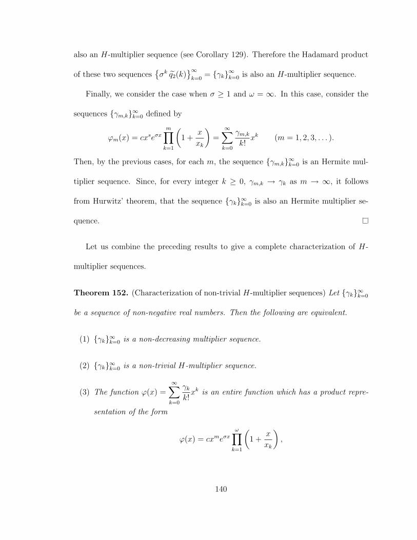
also an H-multiplier sequence (see Corollary 129). Therefore the Hadamard product

of these two sequences{σk q2(k)

}∞k=0

= {γk}∞k=0 is also an H-multiplier sequence.

Finally, we consider the case when σ ≥ 1 and ω = ∞. In this case, consider the

sequences {γm,k}∞k=0 defined by

ϕm(x) = cxseσx

m∏k=1

(1 +

x

xk

)=

∞∑k=0

γm,k

k!xk (m = 1, 2, 3, . . . ).

Then, by the previous cases, for each m, the sequence {γm,k}∞k=0 is an Hermite mul-

tiplier sequence. Since, for every integer k ≥ 0, γm,k → γk as m → ∞, it follows

from Hurwitz’ theorem, that the sequence {γk}∞k=0 is also an Hermite multiplier se-

quence.

Let us combine the preceding results to give a complete characterization of H-

multiplier sequences.

Theorem 152. (Characterization of non-trivial H-multiplier sequences) Let {γk}∞k=0

be a sequence of non-negative real numbers. Then the following are equivalent.

(1) {γk}∞k=0 is a non-decreasing multiplier sequence.

(2) {γk}∞k=0 is a non-trivial H-multiplier sequence.

(3) The function ϕ(x) =∞∑

k=0

γk

k!xk is an entire function which has a product repre-

sentation of the form

ϕ(x) = cxmeσx

ω∏k=1

(1 +

x

xk

),

140

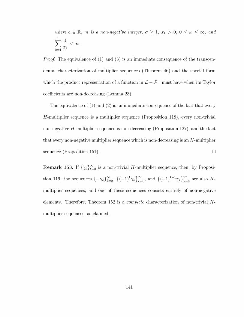
where c ∈ R, m is a non-negative integer, σ ≥ 1, xk > 0, 0 ≤ ω ≤ ∞, andω∑

k=1

1

xk

<∞.

Proof. The equivalence of (1) and (3) is an immediate consequence of the transcen-

dental characterization of multiplier sequences (Theorem 46) and the special form

which the product representation of a function in L − P+ must have when its Taylor

coefficients are non-decreasing (Lemma 23).

The equivalence of (1) and (2) is an immediate consequence of the fact that every

H-multiplier sequence is a multiplier sequence (Proposition 118), every non-trivial

non-negative H-multiplier sequence is non-decreasing (Proposition 127), and the fact

that every non-negative multiplier sequence which is non-decreasing is anH-multiplier

sequence (Proposition 151).

Remark 153. If {γk}∞k=0 is a non-trivial H-multiplier sequence, then, by Proposi-

tion 119, the sequences {−γk}∞k=0,{(−1)kγk

}∞k=0

, and{(−1)k+1γk

}∞k=0

are also H-

multiplier sequences, and one of these sequences consists entirely of non-negative

elements. Therefore, Theorem 152 is a complete characterization of non-trivial H-

multiplier sequences, as claimed.

141

Chapter 6

Linear Operators for Other Polynomial

Sets

6.1 General Polynomial Sets

In this chapter we consider the analogous results of the preceding chapters for other

polynomial sets. We begin in a very general setting and will then apply these results

to various polynomial sets. We begin with the relevant definitions.

Definition 154. A set of polynomials {qk(x)}∞k=0 satisfying

deg(qk(x)) = k (k = 0, 1, 2, . . . ).

is called a simple set of polynomials.

Since we adopt the convention that deg(0) < 0, any simple set of real polynomials

forms a basis for the vector space of real polynomials R[x].

Definition 155. Let Q = {qk(x)}∞k=0 be a simple set of real polynomials and let

{γk}∞k=0 be a sequence of real numbers. Then the TQ-operator associated with the

sequence {γk}∞k=0 is the linear operator defined on R[x] by

TQ[qn(x)] = nqn(x) (n = 0, 1, 2, . . . ).

If the operator TQ has the property that

TQ[p(x)] ∈ L − P whenever p(x) ∈ R[x] ∩ L − P ,

142

then the sequence {γk}∞k=0 is called a multiplier sequence for the simple set Q or, for

brevity, a Q-multiplier sequence. Similarly, if the operator TQ has the property that,

for any real polynomial p(x),

ZC

(TQ[p(x)]

)≤ ZC

(p(x)

),

(where ZC(f(x)) is defined as in Notation 56) then the sequence {γk}∞k=0 is called a

complex zero decreasing sequence for the simple set Q or, for brevity, a Q-CZDS.

The next proposition shows that the complex zero decreasing sequences for a given

simple set are the same as those for another related simple set.

Lemma 156. Let Q = {qk(x)}∞k=0 be a simple set of polynomials and suppose {ck}∞k=0

is a sequence of non-zero real numbers, α ∈ R \ {0}, and β ∈ R. Let Q = {q(x)}∞k=0,

where we define

qk(x) = ck qk(αx+ β) (k = 0, 1, 2, . . . ).

Then {γk}∞k=0 is a Q-CZDS if and only if {γk}∞k=0 is a Q-CZDS.

Proof. Since we have assumed that Q is a simple set of polynomials, {ck}∞k=0 is a

sequence of non-zero real numbers, and α ∈ R is non-zero, it follows that Q is also a

simple set of polynomials.

We will make frequent use of the transformations

x 7−→ αx+ β and x 7−→ x− β

α,

which , since α and β are real and α 6= 0, do not change the number of non-real zeros

of any polynomial.

143

Suppose {γk}∞k=0 is a Q-CZDS and letn∑

k=0

akqk(x) be any real polynomial. Then,

by the definition of qk(x) and by applying the transformation x 7→ x− β

α,

ZC

(n∑

k=0

akqk(x)

)= ZC

(n∑

k=0

akckqk(αx+ β)

)= ZC

(n∑

k=0

akckqk(x)

). (6.1)

Since we have assumed {γk}∞k=0 is a Q-CZDS, we have

ZC

(n∑

k=0

akckqk(x)

)≥ ZC

(n∑

k=0

akckγkqk(x)

). (6.2)

Applying the transformation x 7→ αx+ β yields

ZC

(n∑

k=0

akckγkqk(x)

)= ZC

(n∑

k=0

akγkckqk(αx+ β)

)= ZC

(n∑

k=0

akγkqk(x)

).

(6.3)

Together, (6.1), (6.2), and (6.3) show that {γk}∞k=0 is a Q-CZDS.

Conversely, suppose {γk}∞k=0 is a Q-CZDS and letm∑

k=0

bkqk(x) be any real polyno-

mial. Then, using the fact that ck 6= 0 and applying the transformation x 7→ αx+ β,

we have

ZC

(m∑

k=0

bkqk(x)

)= ZC

(m∑

k=0

bkckckqk(αx+ β)

)= ZC

(m∑

k=0

bkckqk(x)

). (6.4)

Since we have assumed {γk}∞k=0 is a Q-CZDS, we have

ZC

(m∑

k=0

bkckqk(x)

)≥ ZC

(m∑

k=0

bkckγkqk(x)

)= ZC

(m∑

k=0

bkckγkckqk(αx+ β)

). (6.5)

Applying the transformation x 7→ x− β

αyields

ZC

(m∑

k=0

bkckγkckqk(αx+ β)

)= ZC

(m∑

k=0

bkγkqk(x)

). (6.6)

Together, (6.4), (6.5), and (6.6) show that {γk}∞k=0 is a Q-CZDS.

144

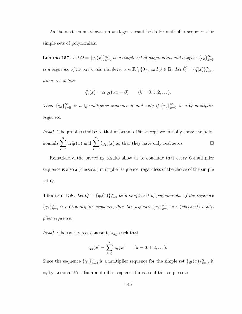
As the next lemma shows, an analogous result holds for multiplier sequences for

simple sets of polynomials.

Lemma 157. Let Q = {qk(x)}∞k=0 be a simple set of polynomials and suppose {ck}∞k=0

is a sequence of non-zero real numbers, α ∈ R \ {0}, and β ∈ R. Let Q = {q(x)}∞k=0,

where we define

qk(x) = ck qk(αx+ β) (k = 0, 1, 2, . . . ).

Then {γk}∞k=0 is a Q-multiplier sequence if and only if {γk}∞k=0 is a Q-multiplier

sequence.

Proof. The proof is similar to that of Lemma 156, except we initially chose the poly-

nomialsn∑

k=0

akqk(x) andm∑

k=0

bkqk(x) so that they have only real zeros.

Remarkably, the preceding results allow us to conclude that every Q-multiplier

sequence is also a (classical) multiplier sequence, regardless of the choice of the simple

set Q.

Theorem 158. Let Q = {qk(x)}∞k=0 be a simple set of polynomials. If the sequence

{γk}∞k=0 is a Q-multiplier sequence, then the sequence {γk}∞k=0 is a (classical) multi-

plier sequence.

Proof. Choose the real constants ak,j such that

qk(x) =k∑

j=0

ak,jxj (k = 0, 1, 2, . . . ).

Since the sequence {γk}∞k=0 is a multiplier sequence for the simple set {qk(x)}∞k=0, it

is, by Lemma 157, also a multiplier sequence for each of the simple sets

145

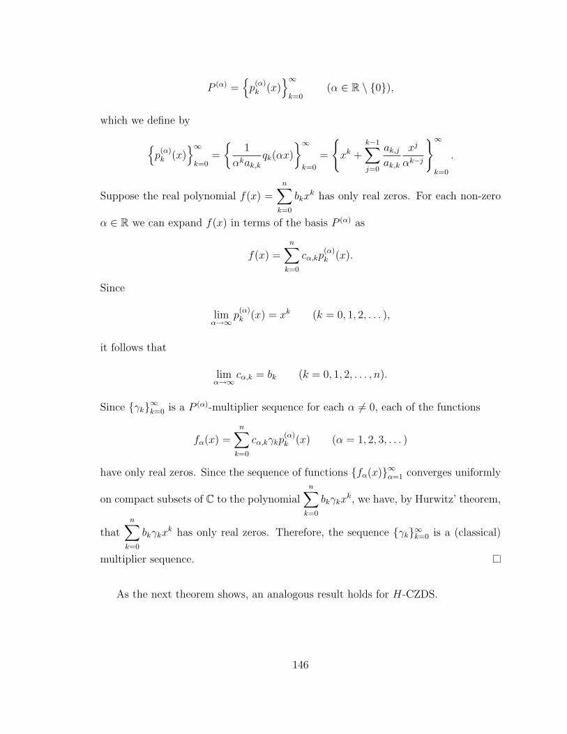
P (α) ={p

(α)k (x)

}∞k=0

(α ∈ R \ {0}),

which we define by

{p

(α)k (x)

}∞k=0

=

{1

αkak,k

qk(αx)

}∞k=0

=

{xk +

k−1∑j=0

ak,j

ak,k

xj

αk−j

}∞k=0

.

Suppose the real polynomial f(x) =n∑

k=0

bkxk has only real zeros. For each non-zero

α ∈ R we can expand f(x) in terms of the basis P (α) as

f(x) =n∑

k=0

cα,kp(α)k (x).

Since

limα→∞

p(α)k (x) = xk (k = 0, 1, 2, . . . ),

it follows that

limα→∞

cα,k = bk (k = 0, 1, 2, . . . , n).

Since {γk}∞k=0 is a P (α)-multiplier sequence for each α 6= 0, each of the functions

fα(x) =n∑

k=0

cα,kγkp(α)k (x) (α = 1, 2, 3, . . . )

have only real zeros. Since the sequence of functions {fα(x)}∞α=1 converges uniformly

on compact subsets of C to the polynomialn∑

k=0

bkγkxk, we have, by Hurwitz’ theorem,

thatn∑

k=0

bkγkxk has only real zeros. Therefore, the sequence {γk}∞k=0 is a (classical)

multiplier sequence.

As the next theorem shows, an analogous result holds for H-CZDS.

146

Theorem 159. Let Q = {qk(x)}∞k=0 be a simple set of polynomials. If the sequence

{γk}∞k=0 is a Q-CZDS, then the sequence {γk}∞k=0 is a (classical) CZDS.

Proof. The proof follows along the same lines as the proof of Theorem 158, except

we note that each of the functions fα(x) satisfy Zc(fα) ≤ Zc(f).

Remark 160. Several remarks are in order.

1. The converse of Theorems 158 and 159 are false. For example, if we take Q = H

to be the set of Hermite polynomials, then, for 0 < r < 1, the sequence{rk}∞

k=0

is a CZDS and a multiplier sequence, but, since it is positive and decreasing,

is not an H-CZDS or an H-multiplier sequence (see Theorem 127 and Remark

128).

2. Since the Hermite polynomials form a simple set of polynomials, we now have

another proof that every H-CZDS is a classical CZDS (Proposition 109). Sim-

ilarly, we have another proof that every H-multiplier sequence is a classical

multiplier sequence (Proposition 118).

3. When studying multiplier sequences (or CZDS) for any simple set Q, we may

restrict our attention to the classical multiplier sequences (or CZDS). Further-

more, several properties of multiplier sequences will carry over to Q-multiplier

sequences, regardless of the choice of Q. For example, the elements of a Q-

multiplier sequence must all have the same sign, or they must alternate signs.

4. The preceding results provide another tool for attempting to characterize the

147

classical CZDS. For example, we mentioned earlier that it is not known whether

the sequence{e−k3

}∞k=0

is a CZDS or not. If we could show that there is a simple

set Q such that{e−k3

}∞k=0

is a Q-CZDS, then it will follow that{e−k3

}∞k=0

is a

classical CZDS.

6.2 Generalized Hermite Polynomials

In this section, we examine linear operators defined on the simple set of generalized

Hermite polynomials Hα ={H(α)

k (x)}∞

k=0defined by the generating relation (2.11).

Since the generalized Hermite polynomials satisfy the differential equation (2.17), we

have the relation(xD − αD2

)[H(α)

n (x)] = nH(α)n (x) (α ∈ R; n = 0, 1, 2, . . . ). (6.7)

Therefore, for α > 0, many of the results we have obtained for the Hermite polyno-

mials which were a consequence of the relation(xD − 1

2D2

)[Hn(x)] = nHn(x) (α ∈ R; n = 0, 1, 2, . . . )

carry over to these generalized Hermite polynomials. For example, the same argument

used to show that sequences of the form

{ϕ(k)

(k(k − 1) · · · (k −m+ 1)

p∏i=1

(k − bi)

)}∞k=0

(bi ≤ m; i = 1, 2, 3, . . . , p)

are H-CZDS can be used to show that these sequences are also Hα-CZDS, where

α > 0 has been fixed. Similarly, the proof of the fact that every non-negative mul-

148

tiplier sequence which is non-decreasing must be an H-multiplier sequence can be

adapted to the setting of Hα-multiplier sequences, where again α > 0 has been fixed.

Instead of reproducing these arguments, we present a more elegant proof which ap-

peals to the results of the previous section.

Lemma 161. Suppose α > 0. Then a sequence of real numbers {γk}∞k=0 is an H-

multiplier sequence if and only if it is an Hα-multiplier sequence. Similarly, a sequence

of real numbers {γk}∞k=0 is an H-CZDS if and only if it is an Hα-CZDS.

Proof. Let us recall the relation between the classical and generalized Hermite poly-

nomials (equation (2.13)),

H(α)k (x) =

(α2

)k/2

Hk

(x√2α

) (α ∈ (R \ {0}) ; k = 0, 1, 2, . . .

).

From this relation and the fact that we have assumed α > 0, we see that this lemma

follows immediately from Lemmas 156 and 157.

By Lemma 161, all of the results of the preceding chapters apply to the simple set

Hα for any α > 0. When α = 0, the set H(0) reduces to the standard basis and the

classical results apply. Let us now investigate the case where α < 0.

Example 162. The sequence {k}∞k=0 is not an Hα-multiplier sequence for any α < 0.

Indeed, the polynomial

H(α)2 (x) + αH(α)

0 (x) = (x2 − α) + α(1) = x2

has only real zeros, while

2H(α)2 (x) + α 0H(α)

0 (x) = 2H(α)2 (x) = 2(x2 − α),

149

which, since α < 0, has two non-real zeros.

We see already that the case α < 0 is very different from the case α > 0. This

should be expected since, in the one case (α > 0), the simple set Hα consists entirely

of polynomials having only simple real zeros while, in the other case (α < 0), the

simple set Hα consists entirely of polynomials having only simple zeros, all of which

lie on the imaginary axis. The next proposition further demonstrates this difference.

Proposition 163. Suppose α < 0 and r > 0. Then the sequence{rk}∞

k=0is an

Hα-CZDS if and only if r ≤ 1.

Proof. Suppose{rk}∞

k=0is an Hα-CZDS and let THα denote the THα-operator asso-

ciated with the sequence{rk}∞

k=0. Then, since

p(x) = H(α)2 (x) + αH(α)

0 (x) = (x2 − α) + α(1) = x2

has only real zeros, we have

THα [p(x)] = r2H(α)2 (x) + αH(α)

0 (x) = r2(x2 − α) + α(1) = r2x2 + α(1− r2) ∈ L − P ,

which, since α < 0, occurs if and only if 1− r2 ≥ 0. Therefore r ≤ 1.

Conversely, suppose 0 < r ≤ 1. If r = 1, then the sequence{rk}∞

k=0= {1}∞k=0 is

clearly an Hα-CZDS. Thus, we may assume 0 < r < 1. Suppose

p(x) =m∑

k=0

akH(α)k (x) ∈ R[x]

and, for any real numbers A and B, define the polynomial fA,B(x) by

fA,B(x) = Ap(x)− xp′(x)−Bp′′(x)

150

By Proposition 68, the inequality ZC

(fA,B(x)

)≤ ZC

(p(x)

)holds whenever A,B ≥ 0

and A ≥ m = deg(q). Since we have assumed α < 0, the inequality

ZC

(− Ap(x) + xp′(x)− αp′′(x)

)= ZC

(− fA,−α(x)

)≤ ZC

(p(x)

)(6.8)

holds whenever A ≥ m. From the relation (6.7) we have

(−A+ xD − αD2)[H(α)

k (x)]

= (−A+ k)H(α)k (x) (k = 0, 1, 2, . . . ).

Thus, we may rewrite inequality (6.8) as

ZC

(m∑

k=0

ak(−A+ k)H(α)k (x)

)≤ ZC

(m∑

k=0

akH(α)k (x)

)(A ≥ m). (6.9)

Note that the sequence{rk}∞

k=0can be interpolated by the function

ϕ(x) = rx = e(ln r)x

which is the uniform limit on compact subsets of C of the sequence of polynomials

(see Lemma 16)

gn

(xn

)=

(1 +

(ln r)x

n

)n

(n = 0, 1, 2, . . . ).

Since we have assumed 0 < r < 1, we have ln r < 0 and, therefore, the zeros of

gn(x) become arbitrarily large and positive as n tends to infinity. By iteration of the

inequality (6.9), we see that there exists an integer N such that the inequality

ZC

(m∑

k=0

akgn

(k

n

)H(α)

k (x)

)≤ ZC

(m∑

k=0

akH(α)k (x)

)

holds whenever n ≥ N . Since the sequence of polynomials{m∑

k=0

akgn

(k

n

)H(α)

k (x)

}∞n=1

151

converge uniformly on compact subsets of C to the polynomialm∑

k=0

akrkH(α)

k (x), we

have by Hurwitz’ theorem,

ZC

(m∑

k=0

akrkH(α)

k (x)

)≤ ZC

(m∑

k=0

akH(α)k (x)

)as desired.

We summarize the results regarding geometric sequences and generalized Hermite

polynomials in the following theorem.

Remark 164. Suppose r ∈ R \ {0}. Then we have shown the following.

1. If α > 0 then{rk}∞

k=0is an Hα-CZDS if and only if |r| ≥ 1 (Corollary 129).

2. If α = 0 then{rk}∞

k=0is an Hα-CZDS for all r 6= 0 (Remark 59).

3. If α < 0 then{rk}∞

k=0is an Hα-CZDS if and only if |r| ≤ 1 (Proposition 163).

The symmetry of these results is quite remarkable and leads one to wonder whether

or not every CZDS which is not an Hα-CZDS for α > 0 must be an Hα-CZDS for

α < 0. This leads us to the following problem.

Problem 165. If {γk}∞k=0 is a multiplier sequence, then does there exists a non-zero

real constant α such that {γk}∞k=0 is an Hα-multiplier sequence? Similarly, if {γk}∞k=0

is a CZDS, then does there exists a non-zero real constant α such that {γk}∞k=0 is an

Hα-CZDS?

We remark that, if {γk}∞k=0 is a multiplier sequence satisfying 0 ≤ γk ≤ γk+1 for

all k, then {γk}∞k=0 is an Hα-multiplier sequence for any α > 0 (see Theorem 152

152

and Lemma 161). Furthermore, if {γk}∞k=0 is a CZDS which can be interpolated by

a polynomial, then {γk}∞k=0 is an Hα-CZDS for any α > 0, since the polynomials

which interpolate CZDS are the same as those that interpolate H-CZDS (Compare

Theorems 63 and 111).

To captivate the reader, we state the following special case of the previous problem.

Problem 166. Suppose α < 0. Is the CZDS

{1

k!

}∞k=0

an an Hα-CZDS?

We remark that, since the function 1/Γ(x + 1) has zeros at each of the negative

integers, we cannot appeal to Proposition 68, as we did in the proof of Proposition

163, and so this problem remains open.

6.3 Laguerre Polynomials

We have seen that there are several interesting results regarding H-multiplier se-

quences, where H is the set of Hermite polynomials. Recall that the Hermite poly-

nomials form an orthogonal set over the interval (−∞,∞) with respect to the weight

function exp(−x2) (see equation (2.8)). In this section we will investigate Q-multiplier

sequences for another orthogonal set of polynomials. The results of this section are

by no means complete, but we include them so that we can compare and contrast the

some of the multiplier sequences for two different orthogonal polynomial sets.

The set of Laguerre polynomials L = {Ln(x)}∞n=0 are explicitly defined by the

equation (see [27, p. 213])

153

Ln(x) =n∑

k=0

(−1)k

(n

k

)xk

k!(n = 0, 1, 2, . . . ). (6.10)

For the convenience of the reader, we list the first few Laguerre polynomials here.

L0(x) = 1

L1(x) = 1− x

L2(x) =1

2(x2 − 4x+ 2)

L3(x) = − 1

3!(x3 − 9x2 + 18x− 6)

L4(x) =1

4!(x4 − 16x3 + 72x2 − 96x+ 24)

L5(x) = − 1

5!(x5 − 25x4 + 200x3 − 600x2 + 600x− 120)

From equation (6.10) it is easy to see that the set of Laguerre polynomials L

forms a simple set of polynomials. Furthermore, it can be shown that the Laguerre

polynomials satisfy (see [27, p. 214])∫ ∞

0

exp(−x)Ln(x)Lm(x) dx =

{0 if m 6= n,1 if m = n.

Thus, the Laguerre polynomials form an orthogonal set over the interval [0,∞) with

respect to the weight function exp(−x). One can also show that the Laguerre poly-

nomials satisfy Laguerre’s differential equation (see [27, p. 214])

nLn(x) = (x− 1)L′n(x)− xL′′n(x) (n = 0, 1, 2, . . . ). (6.11)

Let us now demonstrate that there are non-trivial L-multiplier sequences.

Lemma 167. If the real polynomial p(x) has only real zeros, then the real polynomial

(x− 1)p(x)− xp′(x) also has only real zeros.

154

Proof. By Laguerre’s theorem (Theorem 60), the operator T = 1 + xD preserves

reality of zeros and, therefore, maps the entire Laguerre-Polya class into itself (see

Proposition 71), i.e., if ϕ(x) ∈ L − P , then ϕ(x) + xϕ′(x) ∈ L − P . In particular,

since the function ϕ(x) = −p(x)e−x belongs to the Laguerre-Polya class,

T [ϕ(x)] = −p(x)e−x + x(p(x)e−x − p′(x)e−x)

= e−x((x− 1)p(x)− xp′(x)

)∈ L − P .

Therefore, (x− 1)p(x)− xp′(x) has only real zeros.

Proposition 168. If the polynomial

p(x) =n∑

k=0

akLk(x)

has only real zeros, then

q(x) =n∑

k=0

kakLk(x) ∈ L − P .

That is to say, the sequence {k}∞k=0 is an L-multiplier sequence.

Proof. Let TL denote the TL operator associated with the sequence {k}∞k=0. We claim

that TL = (x− 1)D−xD2. Indeed, since the Laguerre polynomials satisfy Laguerre’s

differential equation (6.11), we have

((x− 1)D − xD2

)[Lk(x)] = kLk(x) = TL[Lk(x)] (k = 0, 1, 2, . . . ).

Since we have assumed p(x) has only real zeros we have, by Rolle’s theorem, that

p′(x) also has only real zeros (or, perhaps, is identically zero). Therefore, by Lemma

155

167, we have

q(x) = (x− 1)p′(x)− xp′′(x) ∈ L − P .

Let us now employ the Hermite-Poulain Theorem (Theorem 37) and Laguerre’s

theorem (Theorem 60) to demonstrate the existence of another L-multiplier sequence.

Proposition 169. If the polynomial

p(x) =n∑

k=0

akLk(x)

has only real zeros, then the polynomial

q(x) =n∑

k=0

(k + 1)akLk(x)

also has only real zeros. That is to say, the sequence {k + 1}∞k=0 is an L-multiplier

sequence.

Proof. Let TL denote the TL-operator associated with the sequence {k + 1}∞k=0. We

claim that TL = 1 + (x− 1)D − xD2. Indeed, since the Laguerre polynomials satisfy

Laguerre’s differential equation (6.11), we have

(1 + (x− 1)D − xD2

)= (1 + k)Lk(x) = TL[Lk(x)] (k = 0, 1, 2, . . . ).

Since we have assumed p(x) has only real zeros we have, by the Hermite-Poulain

Theorem (Theorem 37), that the polynomial p(x)− p′(x) has only real zeros. Thus,

by Laguerre’s theorem (Theorem 60),

156

(1 + xD)[p(x)− p′(x)] =(p(x)− p′(x)

)+ x

d

dx(p(x)− p′(x))

= p(x) + (x− 1)p′(x)− xp′′(x)

= q(x)

has only real zeros, as desired.

So far, we have demonstrated the existence of two L-multiplier sequences, each

of which are also H-multiplier sequences. We will now show that there are a large

number of H-multiplier sequences which are not L-multiplier sequences.

Proposition 170. If α > 1, then the sequence {α+ k}∞k=0 is not an L-multiplier

sequence.

Proof. Fix α > 1 and let TL denote the TL-operator associated with the sequence

{α+ k}∞k=0. We claim that TL = α + (x − 1)D − xD2. Indeed, since the Laguerre

polynomials satisfy Laguerre’s differential equation (6.11), we have

(α+ (x− 1)D − xD2

)[Lk(x)] = (α+ k)Lk(x) = TL[Lk(x)] (k = 0, 1, 2, . . . ).

For any integer n ≥ 2 we, therefore, have

TL [(x+ n)n] = α [(x+ n)n] + (x− 1)D [(x+ n)n]− xD2 [(x+ n)n]

= α(x+ n)n + (x− 1)n(x+ n)n−1 − xn(n− 1)(x+ n)n−2

= (x+ n)n−2((α+ n)x2 + 2nαx+ (α− 1)n2

).

The discriminant of the quadratic polynomial (α+ n)x2 + 2nαx+ (α− 1)n2 is

4n2((1− α)n+ α). (6.12)

157

Since we have assumed α > 1, we have 1−α < 0 and, therefore, we may pick n large

enough that the discriminant (6.12) is negative. Thus, for any such n, TL[(x+n)n] /∈

L − P and, therefore the sequence {α+ k}∞k=0 is not an L-multiplier sequence.

Remark 171. Again we emphasize that this situation is vastly different from that

of the Hermite polynomials H. Indeed, every sequence {α+ k}∞k=0 with α ≥ 0 is an

H-multiplier sequence.

We are inclined to believe that the following problem can be answered in the

affirmative.

Problem 172. Is it true that the sequence {α+ k}∞k=0 is an L-multiplier sequence if

and only if 0 ≤ α ≤ 1?

Remark 173. We remark that if α < 0, then {α+ k}∞k=0 is not a multiplier sequence

and, therefore, cannot be an L-multiplier sequence. Thus, to answer Problem 172 in

the affirmative, it only remains to show that it is true for 0 < α < 1.

6.4 Q-Multiplier Sequences Which Coincide With Multiplier

Sequences

In this section we will characterize all simple sets Q whose multiplier sequences co-

incide with the classical multiplier sequences. First we will need several preparatory

results.

158

Lemma 174. Let n ≥ 1 be an integer and let q(x) be a polynomial of degree n + 1.

If, for every α, β ∈ R, the polynomial

fα,β(x) = αxn + βq(x) (6.13)

has only real zeros, then xn−1 divides q(x).

Proof. If n = 1 then xn−1 = 1 clearly divides q(x). Suppose n > 1 and write

q(x) = an+1xn+1 + anx

n + an−1xn−1 + · · ·+ a0.

By hypothesis,

fα,1(x) = an+1xn+1 + (α+ an)xn + an−1x

n−1 + · · ·+ a0

has only real zeros for any α ∈ R. Thus, for any α ∈ R, the polynomial

hα(x) = xn+1fα,1

(1

x

)= an+1 + (α+ an)x+ an−1x

2 + · · ·+ a0xn+1

and, therefore, its derivative

h′α(x) = α+ an + 2an−1x+ · · ·+ a0(n+ 1)xn

has only real zeros. But this is only possible if deg(h′α(x)) ≤ 1. Thus,

a0 = a1 = · · · = an−2 = 0

and so xn−1 divides q(x).

In particular, the function f(x) given by equation (6.13) in Lemma 174 has a zero

at the origin of multiplicity greater than or equal to n− 1. The next lemma demon-

strates that the two remaining zeros of f(x) are either separated by, or coincident

with, the origin.

159

Lemma 175. Let n ≥ 1 be an integer and let q(x) be a polynomial of degree n + 1.

If, for every α, β ∈ R, the polynomial

fα,β(x) = αxn + βq(x)

has only real zeros, then

q(x) = cxn−1(x− a)(x− b), (6.14)

where a, b, c are real constants, c 6= 0, and ab ≤ 0.

Proof. That q(x) has the form (6.14) is an immediate consequence of Lemma 174 and

the fact that f0,1(x) = q(x) has only real zeros. It only remains to show that ab ≤ 0.

By hypothesis,

fa+b,1/c(x) = (a+ b)xn + xn−1(x− a)(x− b) = xn−1(x2 + ab

)has only real zeros. Thus ab ≤ 0, as desired.

If two real entire functions f and g have the property that any linear combination

(over R) of f and g has only real zeros, then the pair f and g is called a generalized

real pair (see [20, p. 315]). The property of being a generalized real pair is quite

strong (see [20, Chapter VII]). In the next lemma, it is shown that every pair of

consecutive polynomials of a simple set Q form a generalized real pair, provided we

assume a certain class of sequences are Q-multiplier sequences.

Lemma 176. Let Q = {qk(x)}∞k=0 be a simple set of real monic polynomials. If, for

all integers m ≥ 1, the sequence

{k(k − 1)(k − 2) · · · (k −m+ 1)}∞k=0

160

is a Q-multiplier sequence, then for any integer n ≥ 0 and any α, β ∈ R,

fα,β(x) = αqn(x) + βqn+1(x) ∈ L − P . (6.15)

Proof. It will first be shown that each polynomial in the simple set Q has only real

zeros, and this will establish the result when α or β (or both) are equal to zero. Since

q0(x) is a (non-zero) constant function and q1(x) is a linear function, each of these

polynomials have only real zeros. Fix an integer n ≥ 2 and let

p(x) =n∑

k=0

akqk(x) (an 6= 0)

be a polynomial which has only real zeros. Applying the Q-multiplier sequence

{k(k − 1)(k − 2) · · · (k − n+ 1)}∞k=0

to p(x), we see that ann!qn(x), and therefore qn(x), has only real zeros. Thus, for any

integer n ≥ 0, qn(x) has only real zeros.

If α and β are non-zero, then it suffices to show that fγ,1(x) has only real zeros,

where γ =α

β. Write

qn+1(x) = xn+1 + bnxn + bn−1x

n−1 + · · · b0

and

qn(x) = xn + cn−1xn−1 + cn−2x

n−2 + · · · c0.

With this notation, we have that the polynomial

161

h(x) =

(x+

bn + γ(n+ 1)

n+ 1

)n+1

= xn+1 + (bn + γ(n+ 1))xn +n−1∑k=0

dkxk

= qn+1(x) + γ(n+ 1)qn(x) +n−1∑k=0

ekqk(x),

where the dk’s and ek’s are appropriate real constants, has only real zeros. Applying

the Q-multiplier sequence {k(k − 1) · · · (k − n+ 1)}∞k=0 to h(x), we see that

(n+ 1)!qn+1(x) + γ(n+ 1)n!qn(x) = (n+ 1)![γqn(x) + qn+1(x)

]= (n+ 1)!fγ,1(x)

has only real zeros. Therefore, fγ,1(x) has only real zeros, as desired

In the next proposition, we only assume that two types of sequences are multiplier

sequences for a given simple set Q which consists entirely of monic polynomials.

Amazingly, this is enough to conclude that the simple set Q is actually the standard

basis.

Proposition 177. Let Q = {qk(x)}∞k=0 be a simple set of monic polynomials satisfying

q0(x) = 1 and q1(x) = x. If, for all integers m ≥ 1, the sequence

{k(k − 1)(k − 2) · · · (k −m+ 1)}∞k=0 (6.16)

is a Q-multiplier sequence, and if there exists an open interval I containing the origin

such that, for all r ∈ I, the sequence {rk}∞

k=0(6.17)

162

is a Q-multiplier sequence, then Q is the standard basis {xk}∞k=0.

Proof. It will first be shown that q2(x) = x2. By Lemma 176, any linear combination

αq1(x) + βq2(x) = αx+ βq2(x) (α, β ∈ R)

has only real zeros. Thus, by Lemma 175, we can write the monic quadratic polyno-

mial q2(x) in the form

q2(x) = x2 + bx+ c (b, c ∈ R; c ≤ 0).

The polynomial

h(x) =

(x+

b

2

)2

= x2 + bx+b2

4= q2(x) +

(b2 − 4c

4

)q0(x)

has only real zeros. For any non-zero r ∈ I, the sequence {rk−2}∞k=0 is a classical

multiplier sequence. Thus, for any non-zero r ∈ I, the polynomial

hr(x) = q2(x) +

(b2 − 4c

4

)1

r2q0(x) = x2 + bx+ c+

(b2 − 4c

4r2

)has only real zeros. Since we have assumed c ≤ 0, we have b2 − 4c ≥ 0. If b2 − 4c >

0, then one could choose r sufficiently small so that hr(x) has non-real zeros, a

contradiction. Therefore, b2 − 4c = 0 and, since b2 and −4c are both non-negative,

b = 0 = c. That is to say, q2(x) = x2 as desired.

Now let n ≥ 2 be an integer and suppose qk(x) = xk for k = 0, 1, 2, . . . , n. It will

be shown that qn+1(x) = xn+1. By Lemma 176, every linear combination,

αqn(x) + βqn+1(x) = αxn + βqn+1(x) (α, β ∈ R)

has only real zeros. Therefore, by Lemmas 174 and 175, we can write the monic

(n+ 1)st degree polynomial q(x) as

163

qn+1(x) = xn+1 + bxn + cxn−1 (b, c ∈ R; c ≤ 0).

The polynomial

f(x) =

(x+

b

n+ 1

)(n+1)

,

which has only real zeros, can be written in the form

f(x) = qn+1(x) +

(n(n+ 1)

2· b2

(n+ 1)2− c

)qn−1(x) +

n−2∑k=0

akqk(x).

For any non-zero r ∈ I, the sequence{rk−(n+1)k(k − 1)(k − 2) · · · (k − (n− 2))

}∞k=0

is a Q-multiplier sequence. Therefore, for any non-zero r ∈ I, the polynomial

fr(x) =(n+ 1)!

2!qn+1(x) +

(n(n+ 1)

2· b2

(n+ 1)2− c

)(n− 1)!

r2qn−1(x)

=(n+ 1)!

2!

[x2 + bx+ c+

1

r2

(b2

(n+ 1)2− 2c

(n+ 1)!

)]xn−1

=(n+ 1)!

2!

[x2 + bx+ c+

1

r2(n+ 1)2

(b2 − n+ 1

n!2c

)]xn−1

has only real zeros. Since c ≤ 0, it follows that b2− n+ 1

n!2c ≥ 0. If b2− n+ 1

n!2c > 0,

then one could choose r sufficiently small so that fr(x) has non-real zeros, a contra-

diction. Thus b2 − n+ 1

n!2c = 0 and, since both b2 and −n+ 1

n!2c are non-negative,

b = 0 = c. That is to say, qn+1(x) = xn+1 as desired.

Remark 178. It should be noted that both types of sequences in the hypotheses

of Proposition 177 are essential to the conclusion. To see this, we note that the

164

generalized Hermite polynomials H(α) form a simple set of monic polynomials which

satisfy H(α)0 (x) = 1 and H(α)

1 (x) = x.

If α > 0, then any sequence of the form (6.16) is an H(α)-multiplier sequences (see

Lemma 161 and Proposition 116), and H(α) is clearly not equal to the standard basis

when α > 0. Furthermore, we note that Proposition 177 is not contradicted, since

sequences of the form (6.17) are not H(α)-multiplier sequences for any r ∈ (−1, 1)

(see Remark 164).

Similarly, if α < 0, then any sequence of the form (6.17) is an H(α)-multiplier

sequence for any r ∈ [−1, 1] (see Remark 164), and again it is clear that H(α) is

not equal to the standard basis when α < 0. Again we note that Proposition 177 is

not contradicted, since the sequence {k}∞k=0 is not an H(α)-multiplier sequence (see

Example 162).

We are now in a position to completely characterize all simple sets Q whose

multiplier sequences coincide with the classical multiplier sequences.

Theorem 179. Suppose Q = {qk(x)}∞k=0 is a simple set of polynomials which has the

property that every multiplier sequence is also a Q-multiplier sequence. Then there

exists a sequence of non-zero real numbers {ck}∞k=0 and a constant β ∈ R such that

qk(x) = ck (x+ β)k for all integers k ≥ 0.

Proof. Suppose the polynomials of the simple set Q can be written as

qk(x) =k∑

j=0

ak,jxj (k = 0, 1, 2, . . . ).

165

Note that, since Q is a simple set, ak,k 6= 0 for all integers k ≥ 0. Define the simple

set of polynomials Q = {qk(x)} by

qk(x) =1

ak,k

qk

(x− a1,0

a1,1

)(k = 0, 1, 2, . . . ). (6.18)

By hypothesis, the multiplier sequences

{k(k − 1)(k − 2) · · · (k −m+ 1)}∞k=0 (m = 1, 2, 3, . . . )

and {rk}∞

k=0(r ∈ R \ {0})

are Q-multiplier sequences and, by Lemma 156, are therefore Q-multiplier sequences

as well. Furthermore, each polynomial qk(x) is monic and we also have

q0(x) =1

a0,0

q0

(x− a1,0

a1,1

)=

1

a0,0

a0,0 = 1

and

q1(x) =1

a1,1

(a1,1

(x− a1,0

a1,1

)+ a1,0

)= x.

Therefore, by Proposition 177, the simple set Q is equal to the standard basis.

That is to say, qk(x) = xk for all integers k ≥ 0. In light of the definition of the

polynomials qk(x) given in equation (6.18), we have

1

ak,k

qk

(x− a1,0

a1,1

)= xk (k = 0, 1, 2, . . . ).

Therefore, we have

qk(x) = ak,k

(x+

a1,0

a1,1

)k

(k = 0, 1, 2, . . . ),

as desired.

166

Remark 180. By Lemma 156, a sequence is a multiplier sequence if and only if it is

a Q-multiplier sequence, where the simple set Q = {qk(x)}∞k=0 is defined by

qk(x) = ck(x+ β)k (ck ∈ R \ {0}; β ∈ R).

Theorem 179 shows that these are the only simple sets whose multiplier sequences

coincide with the classical multiplier sequences.

References

[1] D. Bleecker and G. Csordas, Hermite expansions and the distribution of zeros of

entire functions , Acta Sci. Math. (Szeged), 67 (2001), 177-196.

[2] J. Borcea, P. Branden and B. Shapiro, Polya-Schur master theorems for

circular domains and their boundaries, 2006, ArXiv Mathematics e-prints,

arXiv:math/0607755

[3] N. G. de Bruijn, An analogue of grace’s apolarity theorem, Nieuw Arch. Wiskunde

23 (1949) 69-76.

[4] N. G. de Bruijn, The roots of trigonometric integrals, Duke J. Math., 17 (1950)

197-226.

[5] F. Cajori, An Introduction to the Theory of Equations, Dover, New York, 1969.

[6] L. Carlitz, A note on hermite polynomials, Amer. Math. Monthly, Vol. 62, No. 9.

(Nov., 1955), pp. 646-647.

167

[7] J. M. Carnicer, J. M. Pena and A. Pinkus, On some zero-increasing operators,

Acta Math. Hungar., Vol 93, No. 3 (Feb. 2002), pp. 173-198.

[8] T. Craven and G. Csordas, The Gauss-Lucas theorem and Jensen polynomials,

Trans. Amer. Math. Soc. 278 (1983), 415-429.

[9] T. Craven and G. Csordas, Jensen polynomials and the Turan and Laguerre in-

equalities, Pacific J. Math. 136 (1989), 241-260.

[10] T. Craven and G. Csordas, Differential operators of infinite order and the dis-

tribution of zeros of entire functions, J. Math. Anal. Appl. 186 (1994), 799-820.

[11] T. Craven and G. Csordas, Complex zero decreasing sequences , Methods Appl.

Anal. 2 (1995), 420-441.

[12] T. Craven and G. Csordas, Composition theorems, multiplier sequences, and com-

plex zero decreasing sequences , in Value Distribution Theory and Related Topics,

Advances in Complex Analysis and Its Applications, Vol. 3, eds. G. Barsegian, I.

Laine and C. C. Yang, Kluwer Press, 2004.

[13] N. K. Govil and G. N. McTume, Some extensions of Enestrom-Kakeya Theorem,

Int. J. Appl. Math. 11 (2002), 245-253.

[14] R. P. Gupta and G. C. Jain. A generalized Hermite distribution and its properties.

SIAM J. Appl. Math., 27 No. 2. (Sept., 1974), 359-363.

168

[15] E. Hille, A Class of reciprocal functions, Ann. of Math. (2) 27 No. 4 (Jun., 1926),

427-464.

[16] A. Iserles and E. B. Saff, Zeros of expansions in orthogonal polynomials, Math.

Proc. Cambridege Philos. Soc. 105 (1989), 559-573.

[17] J. L. W. V. Jensen. Recherches sur la theorie des equations, Acta Math. 36

(1912-1913), 181-195.

[18] H. Ki and Y.-O. Kim. DeBruijn’s question on the zeros of fourier transforms, J.

Anal. Math. 91 (2003), 369-387.

[19] E. Laguerre. Œuvres. Gauther-Villars, Paris, 1 (1898).

[20] B. Ja. Levin, Distribution of Zeros of Entire Functions , Transl. Math. Mono.

Vol. 5, Amer. Math. Soc., Providence, RI, 1964; revised ed. 1980.

[21] E. Makai and P. Turan Hermite expansions and distribution of zeros of polyno-

mials Pupl. Math. Inst. Hungar. Acad. Sci., Ser. A 8 (1963), 157-162.

[22] M. Marden, The Geometry of the Zeros of a Polynomial in a Complex Variable,

American Mathematical Society, New York, 1949.

[23] N. Obreschkoff, Verteilung und Berechnung der Nullstellen Reeller Polynome,

Veb Deutscher Verlag der Wissenschaften, Berlin, 1963.

[24] G. Polya, Uber einen Satz von Laguerre, Lger. Deutsch. Math-Verein. 38 (1929),

161-168.

169

[25] G. Polya, Uber algebraische Gleichungen mit nur reellen Wurzeln, Vierteljchr.

Naturforsch. Ges. Zurich, 61 (1916), 546-548.

[26] G. Polya and J. Schur, Uber zwei Arten von Faktorenfolgen in der Theorie der

algebraischen Gleichungen, J. Reine Angew. Math. 144, 1914, 89-113.

[27] E. Rainville, Special Functions , Chelsea, New York, 1960.

[28] W. Rudin, Real and Complex Analysis , McGraw-Hill, 1987.

[29] P. Turan, Sur l’algebre fonctionnelle, Compt. Rend. du prem. (Aout-2 Septembre

1950) Congr. des Math. Hongr., 27, Akademiai Kiado, Budapest, 1952, 279-290.

[30] P. Turan, Hermite-expansion and strips for zeros of polynomials, Arch. Math. 5

(1954), 148-152.

[31] P. Turan, To the analytic theory of algebraic equations, Izv. Mat. Inst. 3 (1959),

123-133.

[32] P. Turan, Research problems , Pupl. Math. Inst. Hungar. Acad. Sci., Ser. A 6

(1961), 417-423.

[33] H. S. Wilf, Mathematics for the Physical Sciences, Wiley, New York, 1962.

170