Linear Non-Gaussian Structural Equation Models

Linear Non-Gaussian Structural

Equation Models

Shohei Shimizu, Patrik Hoyer and Aapo Hyvarinen

Osaka University, Japan

University of Helsinki, Finland

IMPS 2008, Durham, NH

2

Abstract

• Linear Structural Equation Modeling (linear SEM)

– Analyzes causal relations

• Covariance-based SEM– Uses covariance structure alone for model identification

– A number of indistinguishable models

• Linear non-Gaussian SEM– Uses non-Gaussian structures for model identification

– Makes many models distinguishable

3

SEM and causal analysis

• SEM is often used for causal analysis

based on non-experimental data

• Assumption: the data generating process

is represented by a SEM model

• If the assumption is reasonable, SEM

provides causal information

4

Limitations of covariance-based SEM

• Covariance-based SEM cannot distinguishbetween many models

• Example

x1 x2e1 x1 x2 e2

5

Linear non-Gaussian SEM

• Many observed data are considerably non-

Gaussian (Micceri, 1989; Hyvarinen et al. 2001)

• Non-Gaussian structures of data are useful(Bentler 1983; Mooijaart 1985)

• Non-Gaussianity distinguish between the two

models (Shimizu et al. 2006) :

x1 x2e1 x1 x2 e2

6

Independent component

analysis (ICA)

• Observed random vector x is modeled as

– are independent and non-Gaussian• Zero means and unit variances

– A is a constant matrix• Typically square, # variables = # independent components

• Identifiable up to permutation of the columns(Mooijaart 1985; Comon, 1994)

Asx =

is

7

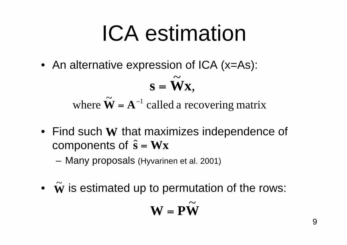
ICA estimation

• An alternative expression of ICA (x=As):

• Find such that maximizes independence of

components of

– Many proposals (Hyvarinen et al. 2001)

• is estimated up to permutation of the rows:

Wxs =ˆ

W~

,~

xWs =

matrixrecoveringacalled~

where1

= AW

WPW~

=

W

8

ICA estimation



components of



Wxs =ˆ

W~

,~

xWs =


where1

= AW

WPW~

=

W

9

ICA estimation



components of



Wxs =ˆ

W~

,~

xWs =


where1

= AW

WPW~

=

W

Discovery of linear non-Gaussian

acyclic models

Shimizu, Hoyer, Hyvarinen and Kerminen (2006)

11

Linear non-Gaussian acyclic

model (LiNGAM)

• Directed acyclic graphs (DAG)– can be arranged in a order k(i)

• Assumptions:– Linearity

– External influences are independent

– and are non-Gaussian

eBxx +=i

ikjk

jijiexbx +=

< )()(

or

ix

ie

12

Goal

• We know

– Data X is generated by

• We do NOT know

– Path coefficients: bij

– Orders k(i)

– External influences: ei

• What we observe is data X only

• Goal– Estimate B and k(i) using data X only!

eBxx +=

13

Key idea

• First, relate LiNGAM with ICA as follows:

• Due to the permutation indeterminacy, ICA

gives:

• Can find a correct P

– The correct permutation is the only one that has no

zeros in the diagonal

xWxBIe

AeeBIx

eBxx

~)(lyequivalent

)(1

==

==

+=

- ICA!

WPW~

=

14

Key idea



gives:




xWxBIe

AeeBIx

eBxx

~)(lyequivalent

)(1

==

==

+=

- ICA!

WPW~

=

15

Key idea



gives:




WPW~

=

xWxBIe

AeeBIx

eBxx

~)(lyequivalent

)(1

==

==

+=

- ICA!

16

Key idea



gives:

• Can find the correct P



WPW~

=

xWxBIe

AeeBIx

eBxx

~)(lyequivalent

)(1

==

==

+=

- ICA!

17

Illustrative example

• Consider the model:

• Goal

– Estimate the path direction between x1 and

x2 observing only x1 and x2

x1 x2e10.6

+=2

1

2

1

2

1

00

6.00

e

e

x

x

x

x

43421

B

18

Perform ICA

• Relation of the LiNGAM model with ICA:

• Due to the permutation indeterminacy, ICA might

give:

=2

1

2

1

10

6.01

x

x

e

e

43421

( )==8.01

10~WPW

xWe~

=

W~

19

Perform ICA

• Relation of the LiNGAM model with ICA:


might give:

=2

1

2

1

10

6.01

x

x

e

e

43421

( )==6.01

10~WPW

xWe~

=

W~

20

Find the correct P

• Find a permutation of the rows of W so that it

has no zeros in the diagonal

• In the example…

=2

1

2

1

10

8.01

x

x

e

e

43421

=2

1

1

2

6.01

10

x

x

e

e

43421

Permute the rows

W W~

0

21

Find the correct P




=2

1

2

1

10

8.01

x

x

e

e

43421

=2

1

1

2

6.01

10

x

x

e

e

43421

Permute the rows

W W~

0

22

Find the correct P




=2

1

2

1

10

6.01

x

x

e

e

43421

=2

1

1

2

6.01

10

x

x

e

e

43421

Permute the rows

W W~

0

0

23

• In practice,

• Heavily penalizes small absolute values in

the diagonal

Find the correct P

( )ii

TWP

PP

1maxˆ =

24

-3 -2 -1 0 1 2 3-3

-2

-1

0

1

2

3

-3 -2 -1 0 1 2 3-3

-2

-1

0

1

2

3

-3 -2 -1 0 1 2 3-3

-2

-1

0

1

2

3

-3 -2 -1 0 1 2 3-3

-2

-1

0

1

2

3

-3 -2 -1 0 1 2 3-3

-2

-1

0

1

2

3

-3 -2 -1 0 1 2 3-3

-2

-1

0

1

2

3

-3 -2 -1 0 1 2 3-3

-2

-1

0

1

2

3

-3 -2 -1 0 1 2 3-3

-2

-1

0

1

2

3

-3 -2 -1 0 1 2 3-3

-2

-1

0

1

2

3

200 1,000 3,000

Number of observations

Num

ber

of

variable

s

10

50

100

Simulations: Estimation of B• Both super- and sub-Gaussian external influences tested

• 5 datasets created for each scatterplot

• B randomly generated at each trial

Generating bij

Estim

ate

d b

ij

25

Prune B (1)

• In practice, due to estimation errors, we

would get:

• Need to find which path coefficients are

actually zeros

+=2

1

2

1

2

1

005.0

65.00

e

e

x

x

x

x

44 344 21

B

26

Find a permutation that gives a

lower triangular matrix

• The LiNGAM model is acyclic

– The matrix B can be permuted to be lower triangular

for some permutation of variables (Bollen, 1989)

• First, find a simultaneous permutation of rows

and columns of B that gives a lower-triangular B

• In practice, find a permutation matrix Q that

minimizes the sum of the elements in its upper

triangular part: ( )=ji

ij

TQBQQ

Q

maxˆ

27











ij

TQBQQ

Q

maxˆ

28











ij

TQBQQ

Q

minˆ

29

Get a lower-triangular B

+=2

1

2

1

2

1

005.0

65.00

e

e

x

x

x

x+=

1

2

1

2

1

2

062.0

05.00

e

e

x

x

x

x

B

• Applying such a simultaneous permutation of the

rows and columns,

• we get a permuted B that is as lower-triangular

as possible

• Set the upper-triangular elements to be zeros

TQBQ

30


+=2

1

2

1

2

1

005.0

65.00

e

e

x

x

x

x+=

1

2

1

2

1

2

065.0

05.00

e

e

x

x

x

x

B


rows and columns,


as possible


TQBQ

31


+=2

1

2

1

2

1

005.0

65.00

e

e

x

x

x

x+=

1

2

1

2

1

2

065.0

05.00

e

e

x

x

x

x

B


rows and columns,


as possible


TQBQ

-0.05

32


+=2

1

2

1

2

1

005.0

65.00

e

e

x

x

x

x+=

1

2

1

2

1

2

065.0

05.00

e

e

x

x

x

x

B


rows and columns,


as possible


TQBQ

0

33

Pruning B (2)

• Once we get a lower-triangular B, the model is

identifiable using covariance-based SEM

• Many existing methods can be used for pruning

the remaining path coefficients

– Wald test, Bootstrapping, Model fit

– Lasso-type estimators (Tibshirani 1996; Zou, 2006) etc.

+=1

2

1

2

1

2

065.0

00

e

e

x

x

x

x

34

1. Estimate B

– ICA + finding the correct row permutation

2. Prune estimated B

1. Find a row-and-column permutation that makes

estimated B lower triangular

2. Prune remaining paths using a covariance-based

method

To summarize the procedure…

x4

x3

x2

x1

x4

x3

x2

x1

x4

x3

x2

x1

1. Estimate B 2. Prune estimated B

35

Summary of the regular LiNGAM

• A linear acyclic model is identifiable based on

non-Gaussianity

• ICA-based estimation works well

– Confidence intervals (Konya et al., in progress)

• Better pruning methods might be developed

– Imposing sparseness in the ICA stage (Zhang & Chang,

2006; Hayashi et al. in progress) like Lasso (Tibshirani 1996)

Some extensions

37

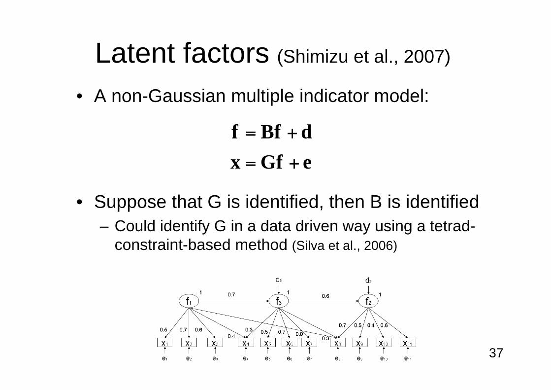
Latent factors (Shimizu et al., 2007)

• A non-Gaussian multiple indicator model:

• Suppose that G is identified, then B is identified

– Could identify G in a data driven way using a tetrad-

constraint-based method (Silva et al., 2006)

eGfx

dBff

+=

+=

38

Latent classes(Shimizu & Hyvarinen, 2008)

• LiNGAM model for each class q:

• ICA mixtures (Lee et al., 2000; Mollah et al., 2006)

Class 1:

Class 2:

0.9

0.2

00

56

x2 x1

x2 x1

qqqqqqqeAìxeìBIxBx +=++= )( - ICA!

39

Unobserved confounders(Hoyer et al., in press

• Can identify and distinguish between more

models

x1 x2 x1 x2

u1

x1 x2

x1 x2

u1

x1 x2

u1

x1 x2

1. 2. 3.

4. 5. 6.

40

Time structures (Hyvarinen et al., 2008)

• Combining LiNGAM and autoregressive model:

– In econometrics: Structural vector autoregression(Swanson & Granger, 1997)

• Changes ordinary AR coefficients based on

instantaneous effects:

)()()(

0

ttt

k

exBx +==

( ) 0for0

>= MBIB ( )matrixAR:M

41

Some variables are Gaussian(Hoyer et al., 2008)

• Consider the model:

• Can identify the path direction

– if either of x1 or e2 is non-Gaussian

• In general, there exist several equivalent models

that entail the same distribution if some are

Gaussian

x2 x1e20.6

42

Some other extensions

• Cyclic models (Lacerda et al., 2008)

– Fewer equivalent models than covariance-based approach

• Nonlinearity (Zhang & Chan, 2007; Sun et al., 2007)

• Model fit statistics are under development

– Non-Gaussian structures

43

Conclusion

• Use of non-Gaussianity in SEM is useful

for model identification

• Many observed data are considerably

non-Gaussian

• The non-Gaussian approach can be a

good option

44

• Most of our papers and Matlab/Octave

code are available on our webpages

• Google will find us!

Linear Non-Gaussian Structural Equation Models

Science

Transcript of Linear Non-Gaussian Structural Equation Models