Linear mixed- effects modeling in SPSSspss.ch/upload/1107355943_LinearMixedEffectsModelling.pdf ·...

AN INTRODUCTION TO THE MIXED PROCEDURE

Linear mixed-effects modeling

in SPSS®

Technica l report

®

Table of contents

Introduction . . . . . . . . . . . . . . . . . . . . . . . . . . . . . . . . . . . . . . . . . . . . . . . . . . . . . . . . . . . . . . . .3

Data preparation for MIXED . . . . . . . . . . . . . . . . . . . . . . . . . . . . . . . . . . . . . . . . . . . . . . . . . . .3

Fitting fixed-effects models with iid residual errors . . . . . . . . . . . . . . . . . . . . . . . . . . . . . . . .6

Example 1 — Fixed-effects model using MIXED . . . . . . . . . . . . . . . . . . . . . . . . . . . . .7

Example 2 — Fixed-effects model using GLM . . . . . . . . . . . . . . . . . . . . . . . . . . . . . . .8

Fitting fixed-effects models with non-iid residual errors . . . . . . . . . . . . . . . . . . . . . . . . . . . . .8

Example 3 — Fixed-effects model with correlated residual errors . . . . . . . . . . . . . . .9

Fitting simple mixed-effects models (balanced design) . . . . . . . . . . . . . . . . . . . . . . . . . . . .10

Example 4 — Simple mixed-effects model with balanced design using MIXED . . .11

Example 5 — Simple mixed-effects model with balanced design using GLM . . . . .12

Example 6 — Variance components model with balanced design . . . . . . . . . . . . . .13

Fitting simple mixed-effects models (unbalanced design) . . . . . . . . . . . . . . . . . . . . . . . . . .14

Example 4a — Mixed-effects model with unbalanced design using MIXED . . . . . .15

Example 5a — Mixed-effects model with unbalanced design using GLM . . . . . . . .16

Example 6a — Variance components model with unbalanced design . . . . . . . . . . .17

Fitting mixed-effects models with subjects . . . . . . . . . . . . . . . . . . . . . . . . . . . . . . . . . . . . . . .17

Example 7 — Fitting random effect*subject interaction using MIXED . . . . . . . . . .18

Example 8 — Fitting random effect*subject interaction using GLM . . . . . . . . . . . .18

Example 9 — Fitting random effect*subject interaction using

SUBJECT specification . . . . . . . . . . . . . . . . . . . . . . . . . . . . . . . . . . . . . . . . . . . . . . . . .19

Example 10 — Using COVTYPE in a random-effects model . . . . . . . . . . . . . . . . . . .20

Multilevel analysis . . . . . . . . . . . . . . . . . . . . . . . . . . . . . . . . . . . . . . . . . . . . . . . . . . . . . . . . . . .21

Example 11 — Multilevel mixed-effects model . . . . . . . . . . . . . . . . . . . . . . . . . . . . . .21

Custom hypothesis tests . . . . . . . . . . . . . . . . . . . . . . . . . . . . . . . . . . . . . . . . . . . . . . . . . . . . . .23

Example 12 — Custom hypothesis testing in mixed-effects model . . . . . . . . . . . . . .23

Covariance structure selection . . . . . . . . . . . . . . . . . . . . . . . . . . . . . . . . . . . . . . . . . . . . . . . .24

Information criteria for Example 9 . . . . . . . . . . . . . . . . . . . . . . . . . . . . . . . . . . . . . . .25

Information criteria for Example 10 . . . . . . . . . . . . . . . . . . . . . . . . . . . . . . . . . . . . . .25

Reference . . . . . . . . . . . . . . . . . . . . . . . . . . . . . . . . . . . . . . . . . . . . . . . . . . . . . . . . . . . . . . . . .26

About SPSS Inc. . . . . . . . . . . . . . . . . . . . . . . . . . . . . . . . . . . . . . . . . . . . . . . . . . . . . . . . . . . . .26

2

L inear mixed-ef fects model ing in SPSS

Technical report

®

3


IntroductionThe linear mixed-effects model (MIXED) procedure in SPSS enables you to fit linear mixed-effects models to data sampled from normal distributions. Recent texts, such as those byMcCulloch and Searle (2000) and Verbeke and Molenberghs (2000), comprehensivelyreviewed mixed-effects models. The MIXED procedure fits models more general than those of the general linear model (GLM) procedure and it encompasses all models in the variancecomponents (VARCOMP) procedure. This report illustrates the types of models that MIXEDhandles. We begin with an explanation of simple models that can be fitted using GLM andVARCOMP, to show how they are translated into MIXED. We then proceed to fit models thatare unique to MIXED.

The major capabilities that differentiate MIXED from GLM are that MIXED handles correlat-ed data and unequal variances. Correlated data are very common in such situations as repeat-ed measurements of survey respondents or experimental subjects. MIXED also handles morecomplex situations in which experimental units are nested in a hierarchy. MIXED can, forexample, process data obtained from a sample of students selected from a sample of schoolsin a district.

In a linear mixed-effects model, responses from a subject are thought to be the sum (linear)of so-called fixed and random effects. If an effect, such as a medical treatment, affects thepopulation mean, it is fixed. If an effect is associated with a sampling procedure (e.g., subjecteffect), it is random. In a mixed-effects model, random effects contribute only to the covariancestructure of the data. The presence of random effects, however, often introduces correlationsbetween cases as well. Though the fixed effect is the primary interest in most studies orexperiments, it is necessary to adjust for the covariance structure of the data. The adjustmentmade in procedures like GLM-Univariate is often not appropriate because it assumes theindependence of the data.

The MIXED procedure solves these problems by providing the tools necessary to estimatefixed and random effects in one model. MIXED is based, furthermore, on maximum likelihood(ML) and restricted maximum likelihood (REML) methods, versus the analysis of variance(ANOVA) methods in GLM. ANOVA methods produce only an optimum estimator (minimumvariance) for balanced designs, whereas ML and REML yield asymptotically efficient estimatorsfor balanced and unbalanced designs. ML and REML thus present a clear advantage overANOVA methods in modeling real data, since data are often unbalanced. The asymptotic normality of ML and REML estimators, furthermore, conveniently allows us to make inferenceson the covariance parameters of the model, which is difficult to do in GLM.

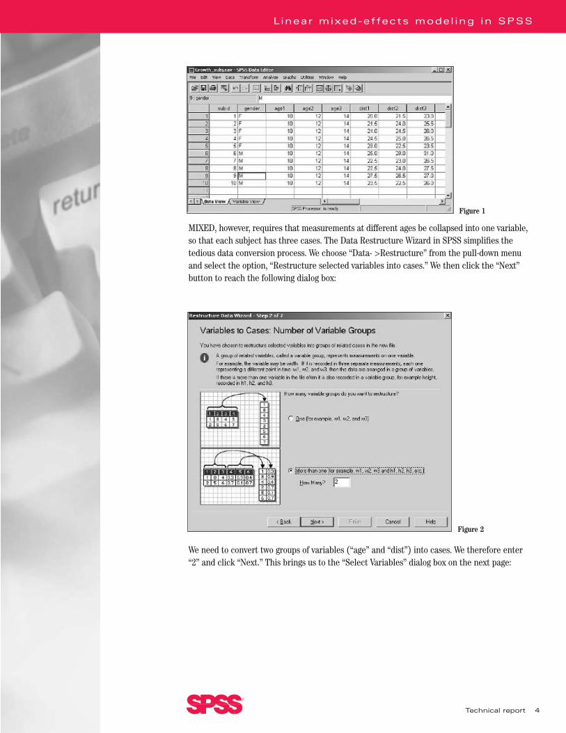
Data preparation for MIXEDMany datasets store repeated observations on a sample of subjects in “one subject per row”format. MIXED, however, expects that observations from a subject are encoded in separaterows. To illustrate, we select a subset of cases from the data that appear in Potthoff and Roy(1964). The data shown in Figure 1 on the next page encode, in one row, three repeatedmeasurements of a dependent variable (“dist1” to “dist3”) from a subject observed at differentages (“age1” to “age3”).

Technical report

®

4

MIXED, however, requires that measurements at different ages be collapsed into one variable,so that each subject has three cases. The Data Restructure Wizard in SPSS simplifies thetedious data conversion process. We choose “Data- >Restructure” from the pull-down menuand select the option, “Restructure selected variables into cases.” We then click the “Next”button to reach the following dialog box:

We need to convert two groups of variables (“age” and “dist”) into cases. We therefore enter“2” and click “Next.” This brings us to the “Select Variables” dialog box on the next page:


Technical report

®

Figure 1

Figure 2

5

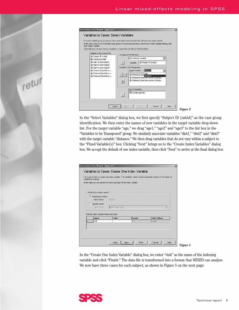
In the “Select Variables” dialog box, we first specify “Subject ID [subid]” as the case group identification. We then enter the names of new variables in the target variable drop-downlist. For the target variable “age,” we drag “age1,” “age2” and “age3” to the list box in the“Variables to be Transposed” group. We similarly associate variables “dist1,” “dist2” and “dist3”with the target variable “distance.” We then drag variables that do not vary within a subject tothe “Fixed Variable(s)” box. Clicking “Next” brings us to the “Create Index Variables” dialogbox. We accept the default of one index variable, then click “Next” to arrive at the final dialog box:

In the “Create One Index Variable” dialog box, we enter “visit” as the name of the indexing variable and click “Finish.” The data file is transformed into a format that MIXED can analyze.We now have three cases for each subject, as shown in Figure 5 on the next page:


Technical report

®

Figure 3

Figure 4

6

We can also perform the conversion using the following syntax:

VARSTOCASES

/MAKE age FROM age1 age2 age3

/MAKE distance FROM dist1 dist2 dist3

/INDEX = visit(3)

/KEEP = subid gender.

The syntax is easy to interpret — it collapses the three age variables into “age” and the threeresponse variables into “distance.” At the same time, a new variable, “visit,” is created to indexthe three new cases within each subject. The last subcommand means that all variables thatare constant within a subject should be kept.

Fitting fixed-effects models with iid residual errorsA fitted model has the form , where is a vector of responses, is the fixed-effects design matrix, is a vector of fixed-effects parameters and is a vector of residualerrors. In this model, we assume that is distributed as , where is an unknowncovariance matrix. A common belief is that . We can use GLM or MIXED to fit amodel with this assumption. Using a subset of the growth study dataset, we illustrate how touse MIXED to fit a fixed-effects model. The following syntax (Example 1) fits a fixed-effectsmodel that investigates the effect of the variables “gender” and “age” on “distance,” which is a measure of the growth rate.


Technical report

®

Figure 5

7

Example 1 — Fixed-effects model using MIXEDSyntax:

MIXED DISTANCE BY GENDER WITH AGE

/FIXED = GENDER AGE | SSTYPE(3)

/PRINT = SOLUTION TESTCOV.

Output:

The syntax in Example 1 produces a “Type III Tests of Fixed Effects” table (Figure 6). Both“gender” and “age” are significant at the .05 level. This means that “gender” and “age” arepotentially important predictors of the dependent variable. More detailed information onfixed-effects parameters may be obtained by using the subcommand /PRINT SOLUTION. The “Estimates of Fixed Effects” table (Figure 7) gives estimates of individual parameters, as well as their standard errors and confidence intervals. We can see that the mean distance for males is larger than that for females. Distance, moreover, increases with age. MIXED also produces an estimate of the residual error variance and its standard error. The /PRINTTESTCOV option gives us the Wald statistic and the confidence interval for the residual errorvariance estimate.


Technical report

®

Figure 6

Figure 7

Figure 8

8

Example 1 is simple — users familiar with the GLM procedure can fit the same model usingGLM.

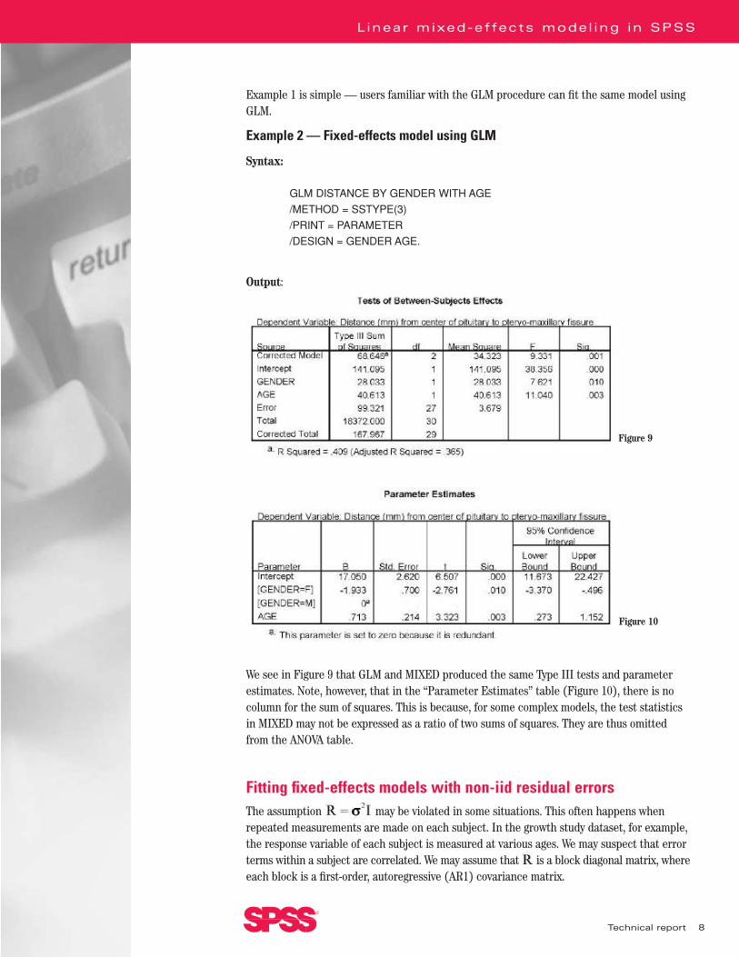
Example 2 — Fixed-effects model using GLM

Syntax:

GLM DISTANCE BY GENDER WITH AGE

/METHOD = SSTYPE(3)

/PRINT = PARAMETER

/DESIGN = GENDER AGE.

Output:

We see in Figure 9 that GLM and MIXED produced the same Type III tests and parameterestimates. Note, however, that in the “Parameter Estimates” table (Figure 10), there is nocolumn for the sum of squares. This is because, for some complex models, the test statisticsin MIXED may not be expressed as a ratio of two sums of squares. They are thus omitted from the ANOVA table.

Fitting fixed-effects models with non-iid residual errorsThe assumption may be violated in some situations. This often happens whenrepeated measurements are made on each subject. In the growth study dataset, for example,the response variable of each subject is measured at various ages. We may suspect that errorterms within a subject are correlated. We may assume that is a block diagonal matrix, whereeach block is a first-order, autoregressive (AR1) covariance matrix.


Technical report

®

Figure 9

Figure 10

9

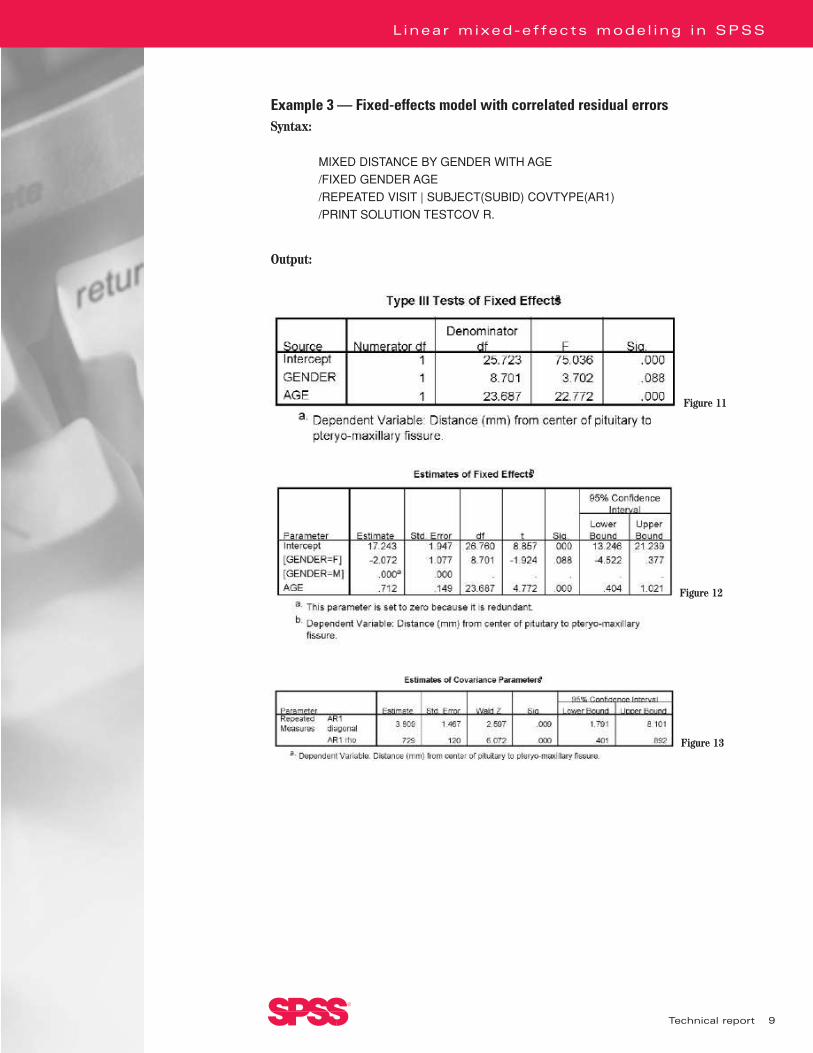
Example 3 — Fixed-effects model with correlated residual errorsSyntax:

MIXED DISTANCE BY GENDER WITH AGE

/FIXED GENDER AGE

/REPEATED VISIT | SUBJECT(SUBID) COVTYPE(AR1)

/PRINT SOLUTION TESTCOV R.

Output:


Technical report

®

Figure 11

Figure 12

Figure 13

10


Technical report

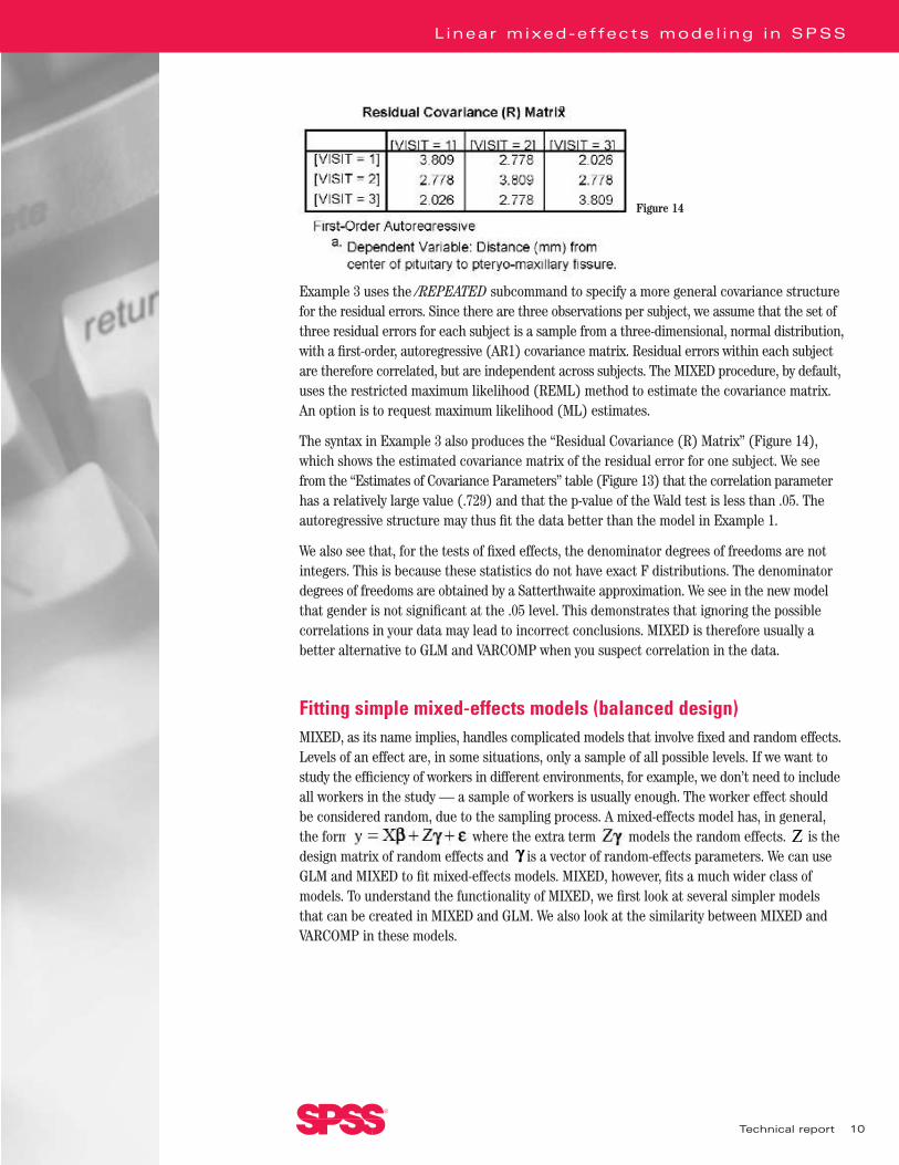
Example 3 uses the /REPEATED subcommand to specify a more general covariance structurefor the residual errors. Since there are three observations per subject, we assume that the set ofthree residual errors for each subject is a sample from a three-dimensional, normal distribution,with a first-order, autoregressive (AR1) covariance matrix. Residual errors within each subjectare therefore correlated, but are independent across subjects. The MIXED procedure, by default,uses the restricted maximum likelihood (REML) method to estimate the covariance matrix.An option is to request maximum likelihood (ML) estimates.

The syntax in Example 3 also produces the “Residual Covariance (R) Matrix” (Figure 14),which shows the estimated covariance matrix of the residual error for one subject. We seefrom the “Estimates of Covariance Parameters” table (Figure 13) that the correlation parameterhas a relatively large value (.729) and that the p-value of the Wald test is less than .05. Theautoregressive structure may thus fit the data better than the model in Example 1.

We also see that, for the tests of fixed effects, the denominator degrees of freedoms are notintegers. This is because these statistics do not have exact F distributions. The denominatordegrees of freedoms are obtained by a Satterthwaite approximation. We see in the new modelthat gender is not significant at the .05 level. This demonstrates that ignoring the possiblecorrelations in your data may lead to incorrect conclusions. MIXED is therefore usually a better alternative to GLM and VARCOMP when you suspect correlation in the data.

Fitting simple mixed-effects models (balanced design)MIXED, as its name implies, handles complicated models that involve fixed and random effects.Levels of an effect are, in some situations, only a sample of all possible levels. If we want tostudy the efficiency of workers in different environments, for example, we don’t need to includeall workers in the study — a sample of workers is usually enough. The worker effect shouldbe considered random, due to the sampling process. A mixed-effects model has, in general,the form where the extra term models the random effects. is thedesign matrix of random effects and is a vector of random-effects parameters. We can useGLM and MIXED to fit mixed-effects models. MIXED, however, fits a much wider class ofmodels. To understand the functionality of MIXED, we first look at several simpler modelsthat can be created in MIXED and GLM. We also look at the similarity between MIXED andVARCOMP in these models.

®

Figure 14

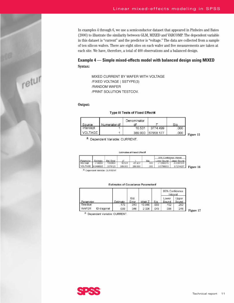
In examples 4 through 6, we use a semiconductor dataset that appeared in Pinheiro and Bates(2000) to illustrate the similarity between GLM, MIXED and VARCOMP. The dependent variablein this dataset is “current” and the predictor is “voltage.” The data are collected from a sampleof ten silicon wafers. There are eight sites on each wafer and five measurements are taken ateach site. We have, therefore, a total of 400 observations and a balanced design.

Example 4 — Simple mixed-effects model with balanced design using MIXEDSyntax:

MIXED CURRENT BY WAFER WITH VOLTAGE

/FIXED VOLTAGE | SSTYPE(3)

/RANDOM WAFER

/PRINT SOLUTION TESTCOV.

Output:

11


Technical report

®

Figure 15

Figure 16

Figure 17

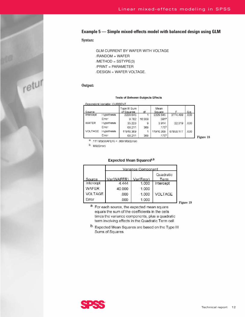
Example 5 — Simple mixed-effects model with balanced design using GLM

Syntax:

GLM CURRENT BY WAFER WITH VOLTAGE

/RANDOM = WAFER

/METHOD = SSTYPE(3)

/PRINT = PARAMETER

/DESIGN = WAFER VOLTAGE.

Output:

12


Technical report

®

Figure 18

Figure 19

Example 6 — Variance components model with balanced designSyntax:

VARCOMP CURRENT BY WAFER WITH VOLTAGE

/RANDOM = WAFER

/METHOD = REML.

Output:

In Example 4, “voltage” is entered as a fixed effect and “wafer” is entered as a random effect.This example tries to model the relationship between “current” and “voltage” using a straightline, but the intercept of the regression line will vary from wafer to wafer according to a normaldistribution. In the Type III tests for “voltage,” we see a significant relationship between “current” and “voltage.” If we delve deeper into the parameter estimates table, the regressioncoefficient of “voltage” is 9.65. This indicates a positive relationship between “current” and“voltage.” In the “Estimates of Covariance Parameters” table (Figure 17), we have estimatesfor the residual error variance and the variance due to the sampling of wafers.

We repeat the same model in Example 5 using GLM. Note that MIXED produces Type III tests for fixed effects only, but GLM includes fixed and random effects. GLM treats all effectsas fixed during computation and constructs F statistics by taking the ratio of the appropriatesums of squares. Mean squares of random effects in GLM are estimates of functions of the variance parameters of random and residual effects. These functions can be recovered from“Expected Mean Squares” (Figure 19). In MIXED, the outputs are much simpler because thevariance parameters are estimated directly using maximum likelihood (ML) or restrictedmaximum likelihood (REML). As a result, there is no random-effect sum of squares.

When we have a balanced design, as in examples 4 through 6, the tests of fixed effects are thesame for GLM and MIXED. We can also recover the variance parameter estimates of MIXEDby using the sum of squares in GLM. In MIXED, for example, the estimate of the residual varianceis 0.175, which is the same as the MS(Error) in GLM. The variance estimate of random effect“wafer” is 0.093, which can be recovered in GLM using the “Expected Mean Squares” table(Figure 19) in Example 5:

Var(WAFER) = [MS(WAFER)-MS(Error)]/40 = 0.093

This is equal to MIXED’s estimate. One drawback of GLM, however, is that you cannot computethe standard error of the variance estimates.

13


Technical report

®

Figure 20

VARCOMP is, in fact, a subset of MIXED. These two procedures, therefore, always provide thesame variance estimates, as seen in examples 4 and 6. VARCOMP only fits relatively simple models. It can only handle random effects that are iid normal. No statistics on fixed effectsare produced. If, therefore, your primary objective is to make inferences about fixed effectsand your data are correlated, MIXED is a better choice.

An important note: due to the different estimation methods that are used, GLM and MIXEDdo not produce the same results. The next section gives an example of such differences.

Fitting simple mixed-effects models (unbalanced design)One situation about which MIXED and GLM disagree is an unbalanced design. To illustratethis, we removed some cases in the semiconductor dataset, so that the design is no longerbalanced.

We then rerun examples 4 through 6 with this unbalanced dataset. The output is shown inexamples 4a through 6a. We want to see whether the three methods — GLM, MIXED andVARCOMP — still agree with each other.

14


Technical report

®

Figure 21

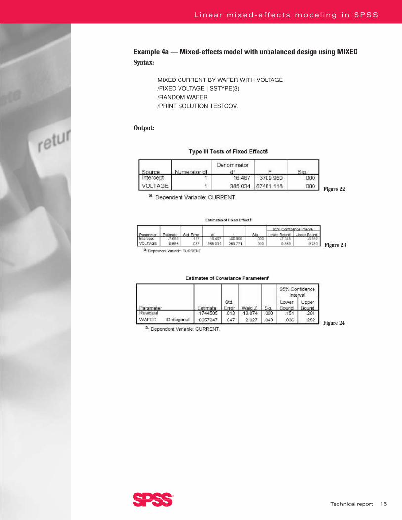
Example 4a — Mixed-effects model with unbalanced design using MIXEDSyntax:

MIXED CURRENT BY WAFER WITH VOLTAGE

/FIXED VOLTAGE | SSTYPE(3)

/RANDOM WAFER


Output:

15


Technical report

®

Figure 22

Figure 23

Figure 24

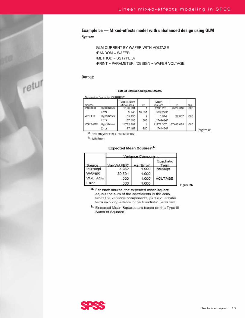
Example 5a — Mixed-effects model with unbalanced design using GLMSyntax:

GLM CURRENT BY WAFER WITH VOLTAGE

/RANDOM = WAFER

/METHOD = SSTYPE(3)

/PRINT = PARAMETER /DESIGN = WAFER VOLTAGE.

Output:

16


Technical report

®

Figure 25

Figure 26

Example 6a — Variance components model with unbalanced designSyntax:

VARCOMP CURRENT BY WAFER WITH VOLTAGE

/RANDOM = WAFER

/METHOD = REML.

Output:

Since the data have changed, we expect examples 4a through 6a to differ from examples 4through 6. We will focus instead on whether examples 4a, 5a and 6a agree with each other.

In Example 4a, the F statistic for the “voltage” effect is 67481.118, but Example 5a gives an F statistic value of 67482.629. Apart from the test of fixed effects, we also see a difference incovariance parameter estimates.

Examples 4a and 6a, however, show that VARCOMP and MIXED can produce the same varianceestimates, even in an unbalanced design. This is because MIXED and VARCOMP use maximumlikelihood or restricted maximum likelihood methods in estimation, while GLM estimates arebased on the method-of-moments approach.

MIXED is generally preferred because it is asymptotically efficient (minimum variance),whether or not the data are balanced. GLM, however, only achieves its optimum behaviorwhen the data are balanced.

Fitting mixed-effects models with subjectsIn the semiconductor dataset, “current” is a dependent variable measured on a batch ofwafers. These wafers are therefore considered subjects in a study. An effect of interest (suchas “site”) may often vary with subjects (“wafer”). One scenario is that the (population) meansof “current” at separate sites are different. When we look at the current measured at thesesites on individual wafers, however, they hover below or above the population mean accordingto some normal distribution. It is therefore common to enter an “effect by subject” interactionterm in a GLM or MIXED model to account for the subject variations.

In the dataset there are eight sites and ten wafers. The site*wafer effect, therefore, has 80parameters, which can be denoted by , i=1...10 and j=1...8. A common assumption is that

’s are assumed to be iid normal with zero mean and an unknown variance. The mean iszero because ’s are used to model only the population variation. The mean of the popula-tion is modeled by entering “site” as a fixed effect in GLM and MIXED. The results of thismodel for MIXED and GLM are shown in examples 7 and 8.

17


Technical report

®

Figure 27

Example 7 — Fitting random effect*subject interaction using MIXEDSyntax:

MIXED CURRENT BY WAFER SITE WITH VOLTAGE

/FIXED SITE VOLTAGE |SSTYPE(3)

/RANDOM SITE*WAFER | COVTYPE(ID).

Output:

Example 8 — Fitting random effect*subject interaction using GLMSyntax:

GLM CURRENT BY WAFER SITE WITH VOLTAGE

/RANDOM = WAFER

/METHOD = SSTYPE(3)

/DESIGN = SITE SITE*WAFER VOLTAGE.

Output:

18


Technical report

®

Figure 28

Figure 29

Figure 30

Since the design is balanced, the results of GLM and MIXED in examples 7 and 8 match. This is similar to examples 4 and 5. We see from the results of Type III tests that “voltage” is stillan important predictor of “current,” while “site” is not. The mean currents at different sitesare thus not significantly different from each other, so we can use a simpler model withoutthe fixed effect “site.” We should still, however, consider a random-effects model, becauseignoring the subject variations may lead to incorrect standard error estimates of fixed effectsor false significant tests.

Up to this point, we examined primarily the similarities between GLM and MIXED. MIXED, in fact, has a much more flexible way of modeling random effects. Using the SUBJECT andCOVTYPE options, Example 9 presents an equivalent form of Example 7.

Example 9 — Fitting random effect*subject interaction using SUBJECT specificationSyntax:

MIXED CURRENT BY SITE WITH VOLTAGE


/RANDOM SITE | SUBJECT(WAFER) COVTYPE(ID).

The SUBJECT option tells MIXED that each subject will have its own set of random parametersfor the random effect “site.” The COVTYPE option will specify the form of the variance covari-ance matrix of the random parameters within one subject. The syntax attempts to specify thedistributional assumption in a multivariate form, which can be written as:

19


Technical report

®

Figure 31

are idd

Figure 32

This assumption is equivalent to that in Example 7 under normality.

One advantage of the multivariate form is that you can easily specify other covariance structuresby using the COVTYPE option. The flexibility in specifying covariance structures helps us tofit a model that better describes the data. If, for example, we believe that the variances of different sites are different, we can specify a diagonal matrix as covariance type and theassumption becomes:

The result of fitting the same model using this assumption is given in Example 10.

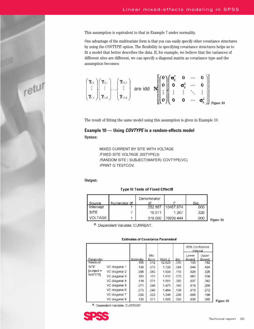
Example 10 — Using COVTYPE in a random-effects modelSyntax:

MIXED CURRENT BY SITE WITH VOLTAGE


/RANDOM SITE | SUBJECT(WAFER) COVTYPE(VC)

/PRINT G TESTCOV.

Output:

20


Technical report

®

are idd

Figure 33

Figure 34

Figure 35

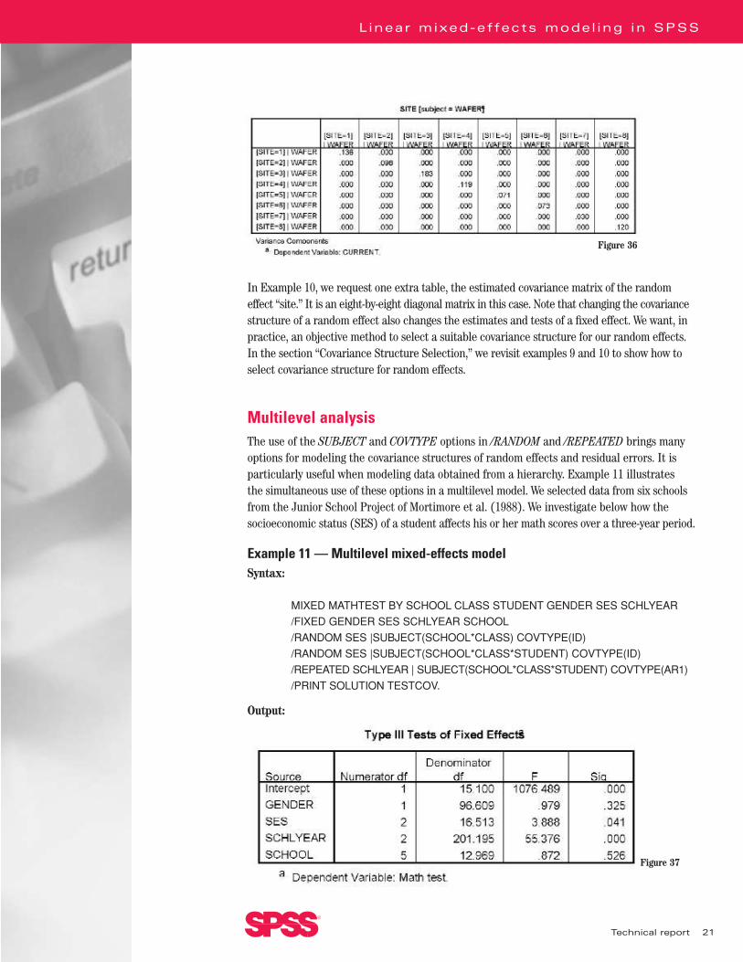
In Example 10, we request one extra table, the estimated covariance matrix of the randomeffect “site.” It is an eight-by-eight diagonal matrix in this case. Note that changing the covariancestructure of a random effect also changes the estimates and tests of a fixed effect. We want, inpractice, an objective method to select a suitable covariance structure for our random effects.In the section “Covariance Structure Selection,” we revisit examples 9 and 10 to show how toselect covariance structure for random effects.

Multilevel analysisThe use of the SUBJECT and COVTYPE options in /RANDOM and /REPEATED brings manyoptions for modeling the covariance structures of random effects and residual errors. It isparticularly useful when modeling data obtained from a hierarchy. Example 11 illustrates the simultaneous use of these options in a multilevel model. We selected data from six schoolsfrom the Junior School Project of Mortimore et al. (1988). We investigate below how thesocioeconomic status (SES) of a student affects his or her math scores over a three-year period.

Example 11 — Multilevel mixed-effects modelSyntax:

MIXED MATHTEST BY SCHOOL CLASS STUDENT GENDER SES SCHLYEAR

/FIXED GENDER SES SCHLYEAR SCHOOL

/RANDOM SES |SUBJECT(SCHOOL*CLASS) COVTYPE(ID)

/RANDOM SES |SUBJECT(SCHOOL*CLASS*STUDENT) COVTYPE(ID)

/REPEATED SCHLYEAR | SUBJECT(SCHOOL*CLASS*STUDENT) COVTYPE(AR1)


Output:

21


Technical report

®

Figure 36

Figure 37

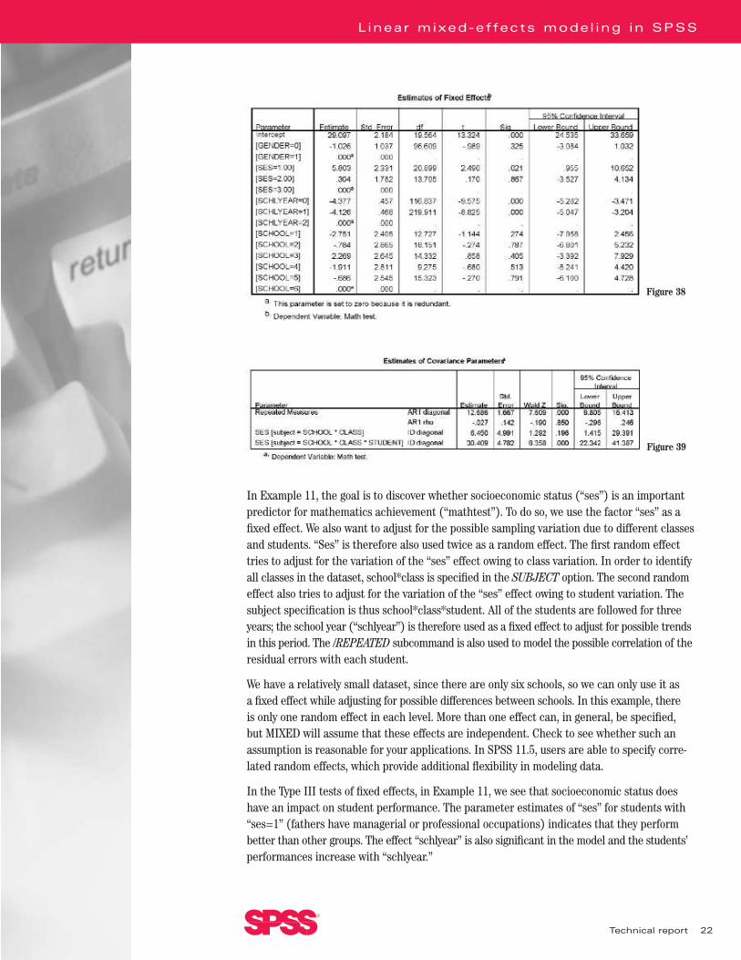
In Example 11, the goal is to discover whether socioeconomic status (“ses”) is an importantpredictor for mathematics achievement (“mathtest”). To do so, we use the factor “ses” as afixed effect. We also want to adjust for the possible sampling variation due to different classesand students. “Ses” is therefore also used twice as a random effect. The first random effecttries to adjust for the variation of the “ses” effect owing to class variation. In order to identifyall classes in the dataset, school*class is specified in the SUBJECT option. The second randomeffect also tries to adjust for the variation of the “ses” effect owing to student variation. Thesubject specification is thus school*class*student. All of the students are followed for threeyears; the school year (“schlyear”) is therefore used as a fixed effect to adjust for possible trendsin this period. The /REPEATED subcommand is also used to model the possible correlation of theresidual errors with each student.

We have a relatively small dataset, since there are only six schools, so we can only use it as a fixed effect while adjusting for possible differences between schools. In this example, there is only one random effect in each level. More than one effect can, in general, be specified, but MIXED will assume that these effects are independent. Check to see whether such anassumption is reasonable for your applications. In SPSS 11.5, users are able to specify corre-lated random effects, which provide additional flexibility in modeling data.

In the Type III tests of fixed effects, in Example 11, we see that socioeconomic status doeshave an impact on student performance. The parameter estimates of “ses” for students with“ses=1” (fathers have managerial or professional occupations) indicates that they performbetter than other groups. The effect “schlyear” is also significant in the model and the students’performances increase with “schlyear.”

22


Technical report

®

Figure 38

Figure 39

From “Estimates of Covariance Parameters” (Figure 39), we notice that the estimate of the“AR1 rho” parameter is not significant, which means that a simple, scaled-identity structuremay be used. For the variation of “ses” due to school*class, the estimate is very small comparedto other sources of variance and the Wald test indicates that it is not significant. We can there-fore consider removing the random effect from the model.

We see from this example that the major advantages of MIXED are that it is able look at differentaspects of a dataset simultaneously and that all of the statistics are already adjusted for alleffects in the model. Without MIXED, we must use different tools to study different aspectsof the models. An example of this is using GLM to study the fixed effect and using VARCOMP tostudy the covariance structure. This is not only time consuming, but the assumptions behindthe statistics are usually violated.

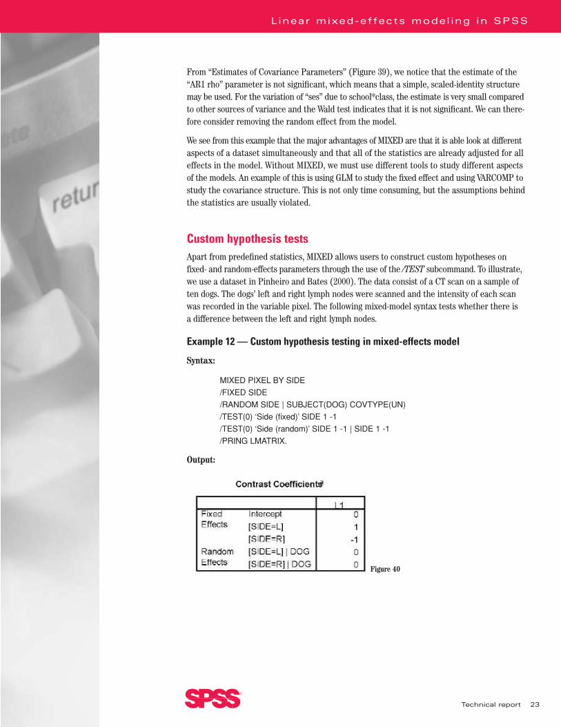
Custom hypothesis testsApart from predefined statistics, MIXED allows users to construct custom hypotheses on fixed- and random-effects parameters through the use of the /TEST subcommand. To illustrate,we use a dataset in Pinheiro and Bates (2000). The data consist of a CT scan on a sample often dogs. The dogs’ left and right lymph nodes were scanned and the intensity of each scanwas recorded in the variable pixel. The following mixed-model syntax tests whether there is a difference between the left and right lymph nodes.

Example 12 — Custom hypothesis testing in mixed-effects model

Syntax:

MIXED PIXEL BY SIDE

/FIXED SIDE

/RANDOM SIDE | SUBJECT(DOG) COVTYPE(UN)

/TEST(0) ‘Side (fixed)’ SIDE 1 -1

/TEST(0) ‘Side (random)’ SIDE 1 -1 | SIDE 1 -1

/PRING LMATRIX.

Output:

23


Technical report

®

Figure 40

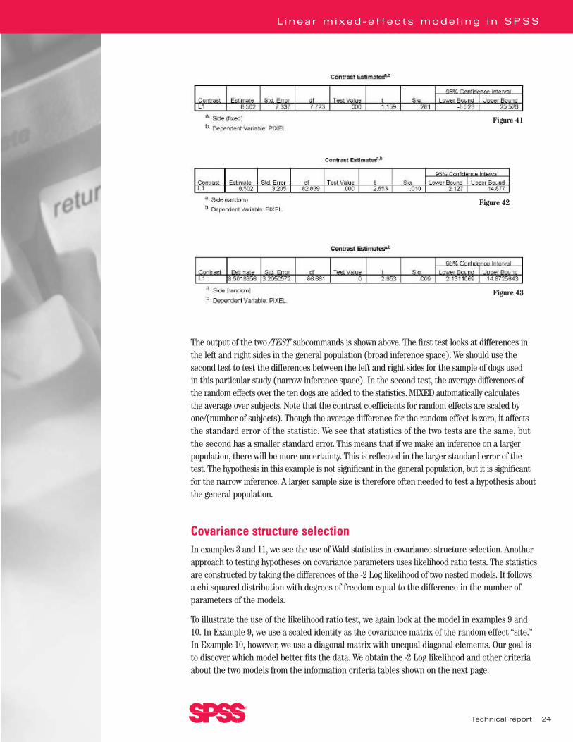
The output of the two /TEST subcommands is shown above. The first test looks at differences inthe left and right sides in the general population (broad inference space). We should use the second test to test the differences between the left and right sides for the sample of dogs used in this particular study (narrow inference space). In the second test, the average differences of the random effects over the ten dogs are added to the statistics. MIXED automatically calculates the average over subjects. Note that the contrast coefficients for random effects are scaled byone/(number of subjects). Though the average difference for the random effect is zero, it affectsthe standard error of the statistic. We see that statistics of the two tests are the same, butthe second has a smaller standard error. This means that if we make an inference on a largerpopulation, there will be more uncertainty. This is reflected in the larger standard error of thetest. The hypothesis in this example is not significant in the general population, but it is significantfor the narrow inference. A larger sample size is therefore often needed to test a hypothesis aboutthe general population.

Covariance structure selectionIn examples 3 and 11, we see the use of Wald statistics in covariance structure selection. Anotherapproach to testing hypotheses on covariance parameters uses likelihood ratio tests. The statisticsare constructed by taking the differences of the -2 Log likelihood of two nested models. It followsa chi-squared distribution with degrees of freedom equal to the difference in the number ofparameters of the models.

To illustrate the use of the likelihood ratio test, we again look at the model in examples 9 and10. In Example 9, we use a scaled identity as the covariance matrix of the random effect “site.”In Example 10, however, we use a diagonal matrix with unequal diagonal elements. Our goal isto discover which model better fits the data. We obtain the -2 Log likelihood and other criteriaabout the two models from the information criteria tables shown on the next page.

24


Technical report

®

Figure 41

Figure 42

Figure 43

Information criteria for Example 9

Information criteria for Example 10

The likelihood ratio test statistic for testing Example 9 (null hypothesis) versus Example 10 is 523.532 - 519.290 = 4.242. This statistic has a chi-squared distribution and the degree of freedom is determined by the difference (seven) in the number of parameters in the two models. The p-value of this statistic is 0.752, which is not significant at level 0.05. Thelikelihood ratio test indicates, therefore, that we may use the simpler model in Example 9.Apart from Wald statistics and likelihood ratio tests, we can also use such information criteriaas Akaike’s Information Criterion (AIC) and Schwarz’s Bayesian Criterion (BIC) to searchfor the best model.

25


Technical report

®

Figure 44

Figure 45

ReferenceMcCulloch, C.E., and Searle, S.R. (2000). Generalized, Linear, and Mixed Models.John Wiley and Sons.

Mortimore, P., Sammons, P., Stoll, L., Lewis, D. and Ecob, R. (1988). School Matters:the Junior Years. Wells, Open Books.

Pinheiro J.C., and Bates, D.M. (2000). Mixed-Effects Models in S and S-PLUS.Springer.

Potthoff, R.F., and Roy, S.N. (1964). “A generalized multivariate analysis of variancemodel useful especially for growth curve problems.” Biometrika, 51:313-326.

Verbeke, G., and Molenberghs, G. (2000). Linear Mixed Models for LongitudinalData. Springer.

About SPSS Inc.SPSS Inc. (Nasdaq: SPSS), headquartered in Chicago, IL, USA, is a multinational computersoftware company providing technology that transforms data into insight through the use of predictive analytics and other data mining techniques. The company’s solutions and productsenable organizations to manage the future by learning from the past, understanding the present and predicting potential problems and opportunities. For more information, visit www.spss.com.

SPSS is a registered trademark and the other SPSS products named are trademarks of SPSS Inc. All other products are trademarks of their respective owners. © Copyright 2002 SPSS Inc.

26


LMEMWP-1002 Technical report

®

Linear mixed- effects modeling in SPSSspss.ch/upload/1107355943_LinearMixedEffectsModelling.pdf ·...

Documents

Transcript of Linear mixed- effects modeling in SPSSspss.ch/upload/1107355943_LinearMixedEffectsModelling.pdf ·...