Linear Matrix Inequalities in Controlstaff.uz.zgora.pl/wpaszke/materialy/ts/slides_1print.pdf ·...

$: Linear Matrix Inequalities in Controlstaff.uz.zgora.pl/wpaszke/materialy/ts/slides_1print.pdf · Linear Matrix Inequalities in Control Bart lomiej Sulikowski, Wojciech Paszke {b.sulikowski,$
Linear Matrix Inequalities in Control

Bart lomiej Sulikowski, Wojciech Paszke

{b.sulikowski, w.paszke}@issi.uz.zgora.plInstitute of Control and Computation Engineering

University of Zielona Gora, POLAND

Zielona Gora, Poland, November 2005

Bart lomiej Sulikowski, Wojciech Paszke Linear Matrix Inequalities in Control

Outline

1. Linear Systems Stability - Background

2. Linear Matrix Inequalities (LMIs)

3. Numerical and analytical solutions to LMIs

4. Geometry of LMIs

5. Bilinear Matrix Inequalities (BMIs)

6. Useful lemmas

7. Control problems solved with LMIs

I Stability investigationI Controller design

8. Standard LMI problems

9. D-Stability

10. Robust stability problem

11. Concluding remarks


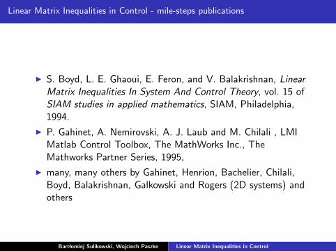
Linear Matrix Inequalities in Control - mile-steps publications

I S. Boyd, L. E. Ghaoui, E. Feron, and V. Balakrishnan, LinearMatrix Inequalities In System And Control Theory, vol. 15 ofSIAM studies in applied mathematics, SIAM, Philadelphia,1994.

I P. Gahinet, A. Nemirovski, A. J. Laub and M. Chilali , LMIMatlab Control Toolbox, The MathWorks Inc., TheMathworks Partner Series, 1995,

I many, many others by Gahinet, Henrion, Bachelier, Chilali,Boyd, Balakrishnan, Galkowski and Rogers (2D systems) andothers


Linear Matrix Inequalities in Control - available solvers

I Matlabr LMI Control Toolbox - in Matlab 7 the LMIControl Toolbox has been incorporated into the RobustControl Toolbox

I Scilab LMI Toolbox

I SeDuMi (+ YALMIP)

I others (plenty of those released lately, indeed any SDP solvercan be used to solve LMI )


Linear System Stability

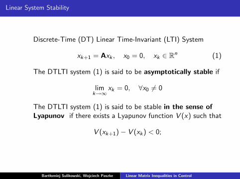
Discrete-Time (DT) Linear Time-Invariant (LTI) System

xk+1 = Axk , x0 = 0, xk ∈ Rn (1)

The DTLTI system (1) is said to be asymptotically stable if

limk→∞

xk = 0, ∀x0 6= 0

The DTLTI system (1) is said to be stable in the sense ofLyapunov if there exists a Lyapunov function V (x) such that

V (xk+1)− V (xk) < 0;



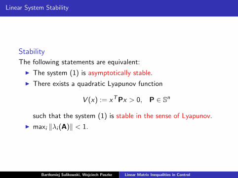
Stability

The following statements are equivalent:

I The system (1) is asymptotically stable.

I There exists a quadratic Lyapunov function

V (x) := xT Px > 0, P ∈ Sn

such that the system (1) is stable in the sense of Lyapunov.

I maxi ‖λi (A)‖ < 1.



Lyapunov Stability Test

Given the system (1) find if there exists a matrix P ∈ Sn such that

a) V (x) := xT Px > 0;∀x 6= 0

b) V (xk+1)− V (xk) < 0; ∀xk+1 = Axk , x 6= 0

Remarks

V (x) := xT Px > 0, ∀x 6= 0 ⇒ P > 0

V (xk+1) = xTk+1Pxk+1 = xT

k AT PAxk

therefore

V (xk+1)− V (xk) = xTk AT PAxk − xT

k Pxk

V (xk+1)− V (xk) = xTk

(AT PA− P

)xk

finally

V (xk+1)− V (xk) < 0 if, and only if AT PA− P < 0



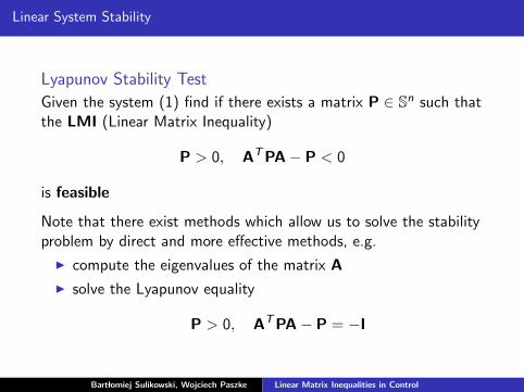
Lyapunov Stability Test

Given the system (1) find if there exists a matrix P ∈ Sn such thatthe LMI (Linear Matrix Inequality)

P > 0, AT PA− P < 0

is feasible

Note that there exist methods which allow us to solve the stabilityproblem by direct and more effective methods, e.g.

I compute the eigenvalues of the matrix A

I solve the Lyapunov equality

P > 0, AT PA− P = −I


Linear Matrix Inequalities

A linear matrix inequality (LMI) is an expression of the form (thecanonical form)

F(x) := F0 + x1F1 + · · ·+ xnFn < 0

where

I x = (x1, . . . , xn) - vector of unknown scalar entries (decisionvariables)

I F0, . . . , Fn - known symmetric matrices

I < 0’ - negative definiteness (in many publications ≺ 0 for thematrix notation is used instead of < 0 - depends on you!)


Features

LMIs have several intrinsic and attractive features

1. An LMI is convex constraint on x (a convex feasibility set). That is,the set S := {x : F(x) < 0} is convex. Indeed, if x1, x2 ∈ S andα ∈ (0, 1) then

F(αx1 + (1− α)x2) = αF(x1) + (1− α)F(x2) > 0

where in the equality we used that F is affine and the inequalityfollows from the fact that α ≥ 0 and (1− α) ≥ 0.

2. While the constraint is matrix inequality instead of a set of scalarinequalities like in linear programming (LP), a much wider class offeasibility sets can be considered.

3. Thirdly, the convex problems involving LMIs can be solved withpowerful interior-point methods. In this case ”solved” means thatwe can find the vector of the decision variables x that satisfies theLMI, or determine that no solution exists.


Example - part 1

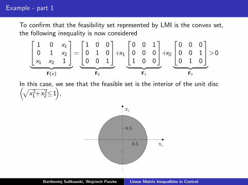
To confirm that the feasibility set represented by LMI is the convex set,the following inequality is now considered 1 0 x1

0 1 x2

x1 x2 1

︸︷︷︸

F(x)

=

1 0 00 1 00 0 1

︸︷︷︸

F0

+x1

0 0 10 0 01 0 0

︸︷︷︸

F1

+x2

0 0 00 0 10 1 0

︸︷︷︸

F2

>0

In this case, we see that the feasible set is the interior of the unit disc(√x21+x2

2≤1)

,

x1

x2

0.5

0.5


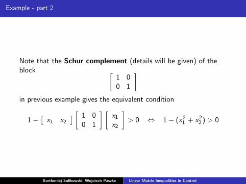
Example - part 2

Note that the Schur complement (details will be given) of theblock [

1 00 1

]in previous example gives the equivalent condition

1−[

x1 x2

] [ 1 00 1

] [x1

x2

]> 0 ⇔ 1− (x2

1 + x22 ) > 0


Other properties

F(x) > 0 is equivalent to –F(x) < 0

F(x) < G(x) is equivalent to F(x) – G(x) < 0

F1(x) < 0, F2(x) < 0 is equivalent to diag(F1(x), F2(x)

)< 0

F(x) < 0, G(y) < 0 is equivalent to diag(F1(x), G(y)

)< 0


Example

Two convex sets described by the previous example and

x1 + 0.5 > 0

are given. They can be expressed by the LMI of the form1 0 x1 00 1 x2 0x1 x2 1 00 0 0 x1 + 0.5

> 0

which represents the convex set depicted below (the intersection ofhyperplane and the interior of the unit circle).

x1

x2

0.5

0.5


Linear Matrix Inequalities cont.

Consider the stability condition for continuous 1D system described byx(t) = Ax(t), which states that the system is stable iff there exists a

matrix P > 0 such that the LMI of AT P + PA < 0 is satisfied. Assumethat n = 2. To present it in the canonical form note that

A =

[a11 a12

a21 a22

], P = PT =

[p11 p12

p12 p22

]Next, the multiplication due to the structures of matrices A and P

provides the following inequality (note that since aij and pkl are scalarsthen aijpkl = pklaij)[

2p11a11 + 2p12a21 p12(a11 + a22) + p22a21 + p11a12

p12(a11 + a22) + p22a21 + p11a12 2p12a12 + 2p22a22

]< 0

or write it in the canonical form as

p11

[2a11 a12

a12 0

]+p12

[2a21 a22 + a11

a22 + a11 2a12

]+p22

[0 a21

a21 2a22

]< 0


Numerical Solution: Interior-point Algorithm

• Basic ideaI Construct a barrier function φ(x) that is well

defined for strict feasible x and is −ε (where−∞ < ε � 0) only at the optimal x = x∗ e.g.

φ(x) = − log det (F (x)) = log det(F−1(x)

)I Generate a sequence {x(k)} so that

limk→∞

φ(x(k)) = −γ

I Stop if φ(x(k)) is negative enough

• polynomial-time algorithm - number of flops boundedby mn3 log (C/ε) (for accuracy < ε)

where m is row size of the LMI, n denotes number of

decision variables and C is a scaling factor.

I unconstrained optimization problem

min f (x) = min f0(x) + µφ(x)

= cT x − µ log det (F (x))

I Application of the Newton-likemethod

Hk∆xk = −tk

x*

x(1)


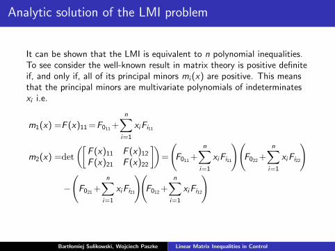
Analytic solution of the LMI problem

It can be shown that the LMI is equivalent to n polynomial inequalities.To see consider the well-known result in matrix theory is positive definiteif, and only if, all of its principal minors mi (x) are positive. This meansthat the principal minors are multivariate polynomials of indeterminatesxi i.e.

m1(x) =F (x)11 =F011 +n∑

i=1

xiFi11

m2(x) =det([

F (x)11 F (x)12

F (x)21 F (x)22

])=

(F011 +

n∑i=1

xiFi11

)(F022 +

n∑i=1

xiFi22

)

−

(F021 +

n∑i=1

xiFi21

)(F012 +

n∑i=1

xiFi12

)


Analytic solution of the LMI problem - cont.

mk(x) =det

F (x)11 · · · F (x)1k

.... . .

...F (x)k1 · · · F (x)kk

mn(x) =det(F(x)) =det

F (x)11 · · · F (x)1n

.... . .

...F (x)n1 · · · F (x)kn

where F (x)kl denotes the element on k-th row and l-th column ofF(x).


Analytic solution of the LMI problem - an example

Consider again the problem of finding a block-diagonal matrixP > 0 (P = diag (Ph, Pv )) such that the following LMI

AT PA− P < 0

or− AT PA + P > 0 (2)

is satisfied. Since P = diag(x1, x2) and the matrix A is given by

A =

[a11 a12

a21 a22

]=

[0.4942 0.57060.1586 0.4662

]


Analytic solution of the LMI problem - an example

The solution of the LMI (2) is equivalent to the solution of the setof inequalities

m1(x)=− x1(a211 − 1)− x2a

221 = 0.75576636x1 − 0.02515396x2 > 0

m2(x)=− x1(a211 − 1)− x2a

221 = 0.32558436x1 + 0.78265756x2 > 0

m3(x)=(−x1(a2

11 − 1)− x2a221

)(−x1a

212 − x2(a2

22 − 1))

−(−x1a12a11 − x2a22a21)(−x1a12a11 − x2a22a21)

=− 0.32558436x21 + 0.5579956166x1x2 − 0.02515396x2

2 > 0

(3)

withx1 > 0 and x2 > 0 (4)


On the other hand, recall that the LMI is a convex set in Rn defined as

F =

{x ∈ Rn : F(x) = F0 +

n∑i=1

xiFi > 0

}

which can be described in terms of principal minors as

F = {x ∈ Rn : mi (x) ≥ 0, i = 1, . . . , n}

Hence the inequalities (3) and (4) describe the convex set

x1

p1

p2

x2


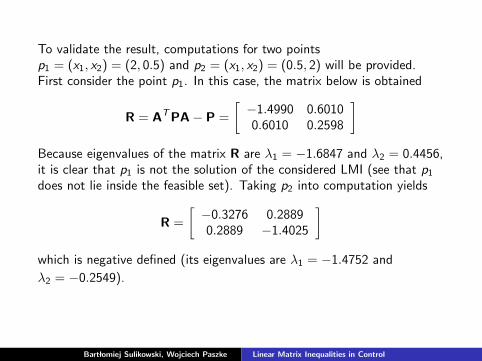
To validate the result, computations for two pointsp1 = (x1, x2) = (2, 0.5) and p2 = (x1, x2) = (0.5, 2) will be provided.First consider the point p1. In this case, the matrix below is obtained

R = AT PA− P =

[−1.4990 0.60100.6010 0.2598

]Because eigenvalues of the matrix R are λ1 = −1.6847 and λ2 = 0.4456,it is clear that p1 is not the solution of the considered LMI (see that p1

does not lie inside the feasible set). Taking p2 into computation yields

R =

[−0.3276 0.28890.2889 −1.4025

]which is negative defined (its eigenvalues are λ1 = −1.4752 and

λ2 = −0.2549).


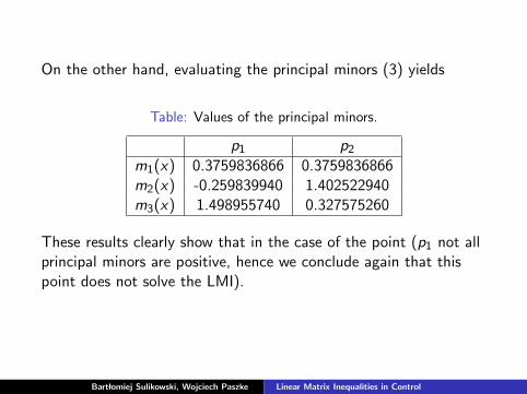
On the other hand, evaluating the principal minors (3) yields

Table: Values of the principal minors.

p1 p2

m1(x) 0.3759836866 0.3759836866m2(x) -0.259839940 1.402522940m3(x) 1.498955740 0.327575260

These results clearly show that in the case of the point (p1 not allprincipal minors are positive, hence we conclude again that thispoint does not solve the LMI).


Geometry of the LMI

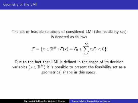
The set of feasible solutions of considered LMI (the feasibility set)is denoted as follows

F ={x ∈ RM : F (x) = F0 +

M∑i=1

xiFi < 0}

Due to the fact that LMI is defined in the space of its decisionvariables (x ∈ RM) it is possible to present the feasibility set as a

geometrical shape in this space.


For the positive (non-negative) definiteness of F (x) it is requiredthat all of its diagonal minors to be positive (non-negative).

For the negative (non-positive) definiteness of F (x) it is requiredthat its diagonal minors of odd minors to be negative

(non-positive) and the minors of even degree to be positive(non-negative) respectively.

It is straightforward to see that the diagonal minors aremulti-variable polynomials of variables xi . So the LMI set can be

described as

F(x) ={x ∈ RM : fi (x) > 0, i = 1, ..,M

}which is a semi-algebraic set. Moreover, it is a convex set.


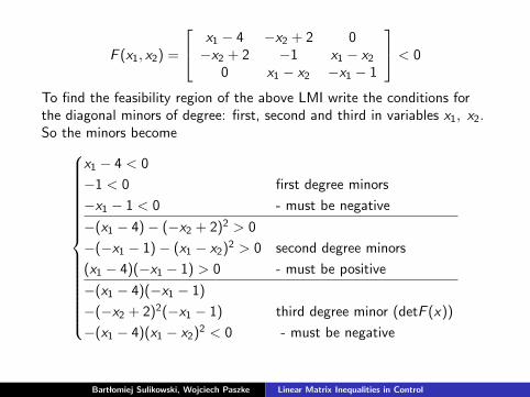
F (x1, x2) =

x1 − 4 −x2 + 2 0−x2 + 2 −1 x1 − x2

0 x1 − x2 −x1 − 1

< 0

To find the feasibility region of the above LMI write the conditions forthe diagonal minors of degree: first, second and third in variables x1, x2.So the minors become

x1 − 4 < 0

−1 < 0 first degree minors

−x1 − 1 < 0 - must be negative

−(x1 − 4)− (−x2 + 2)2 > 0

−(−x1 − 1)− (x1 − x2)2 > 0 second degree minors

(x1 − 4)(−x1 − 1) > 0 - must be positive

−(x1 − 4)(−x1 − 1)

−(−x2 + 2)2(−x1 − 1) third degree minor (detF (x))

−(x1 − 4)(x1 − x2)2 < 0 - must be negative


a) b)

Figure: The solutions for the first (a) and second (b) degree minors

a) b)

Figure: The solutions for the third (a) degree minors and the feasibilityregion for the considered LMI (b)


ConclusionIt is straightforward to see that the feasibility region is the

⋂of the

regions which satisfy the constrains due to corresponding minors.


Matlab solution (script test0.m provides x1 = 1.6667,x2 = 1.8333). Refer to the figure

Figure: The feasibility region and the Matlab solution


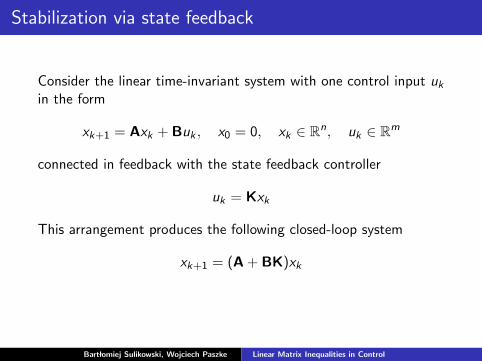
Stabilization via state feedback

Consider the linear time-invariant system with one control input uk

in the form

xk+1 = Axk + Buk , x0 = 0, xk ∈ Rn, uk ∈ Rm

connected in feedback with the state feedback controller

uk = Kxk

This arrangement produces the following closed-loop system

xk+1 = (A + BK)xk


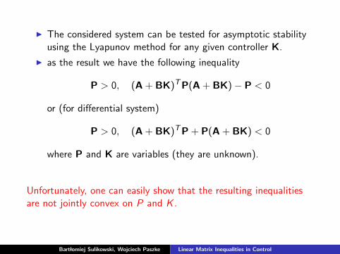
I The considered system can be tested for asymptotic stabilityusing the Lyapunov method for any given controller K.

I as the result we have the following inequality

P > 0, (A + BK)T P(A + BK)− P < 0

or (for differential system)

P > 0, (A + BK)T P + P(A + BK) < 0

where P and K are variables (they are unknown).

Unfortunately, one can easily show that the resulting inequalitiesare not jointly convex on P and K .


Bilinear Matrix Inequality

Bilinear Matrix Inequality (BMI) has the following form

F(x , y) = F(x , y)T = F0 +n∑

i=1

xiFi +m∑

j=1

yjGj +n∑

i=1

m∑j=1

xiyjHij < 0

where

I x = (x1, . . . , xn), x ∈ Rn and y = (x1, . . . , ym), y ∈ Rm arethe variables

I symmetric matrices F0, Fi, i = 1, . . . , n, Gj, j = 1, . . . ,m andHij, i = 1, . . . , n, j = 1, . . . ,m are given data.

RemarkUnfortunately, BMIs are in general highly non-convex optimizationproblems, which can have multiple local solutions, hence solving ageneral BMI was shown to be NP-hard problem


Bilinear Matrix Inequality

Consider the following bilinear inequality

1− xy > 0 (5)

It is clear that (5) does not represent a convex set. To see this, considertwo points on xy -plane which satisfy (5), e.g. p1 = (x1, y1) = (0.2, 2) andp2 = (x2, y2) = (4, 0.2)

0 0.5 1 1.5 2 2.5 3 3.5 4 4.5 50

0.5

1

1.5

2

2.5

3

3.5

4

4.5

5

p1

p2

p3

x

y

Obviously, the point in the half way between the two values, i.e.

p3 =1

2(0.2, 2) +

1

2(4, 0.2) = (2.1, 1.1)

does not satisfy (5).


Can BMIs be written in the form of LMIs?

• Consider the following BMI x2(−13−5x1+x2) x2 0x2 x1 00 0 x1(−13−5x1+x2)−x2

>0

I feasibility set is convex !

I the LMI form can be obtained[−1 + x1 1

1 −1− 518

x1 + 118

x2

]> 0

1 2 3 4 5 6 7 8 9 1040

50

60

70

80

90

100

x1

x2


Methods to reformulate hard problems into LMIsAn important fact from the matrix theory

If some matrix F(x) is positive defined than zT F(x)z > 0, ∀z 6= 0,z ∈ Rn. Assume now that z = My where M is any given nonsingularmatrix, hence

zT F(x)z > 0

implies thatyT MT F(x)My > 0

This means that some rearrangements of the matrix elements do notchange the feasible set of LMIs.


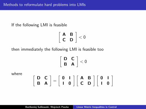
Methods to reformulate hard problems into LMIs

If the following LMI is feasible[A BC D

]< 0

then immediately the following LMI is feasible too[D CB A

]< 0

where [D CB A

]=

[0 II 0

] [A BC D

] [0 II 0

]


Change of variables

In the case of the Lyapunov inequalities, the fact that the niceinequalities previously obtained are functions of X := P−1,and not P,suggests that we might start by rewriting the inequalities in terms of X.

X > 0, X(A + BK)T + (A + BK)X < 0

We then manipulate the second inequality by expanding theproducts

AX + XAT + BKX + XKT BT < 0.


Change of variables

I introduce the new unknown N = KX

I to eliminate the matrix K, or, in other words, K can beexplicitly expressed in terms of other unknowns, by solving thechange of variable equation for the unknown K. Thisproduces K = LX−1

I finally, we have to solve the following inequality

X > 0, AX + XAT + BL + LT BT < 0,


Methods to reformulate hard problems into LMIsSchur complement formula

Quadratic but convex inequality can be converted into the LMI formusing the Schur complement formula given by the following Lemma.

Let A ∈ Rn×n and C ∈ Rm×m be symmetric matrices and A � 0 then

C + BT A−1B < 0

if and only if

U =

[−A B

BT C

]< 0 or, equivalently, U =

[C BT

B −A

]< 0

The matrix C + BT A−1B is called the Schur complement of A in U.The identical result holds for a positive defined case.


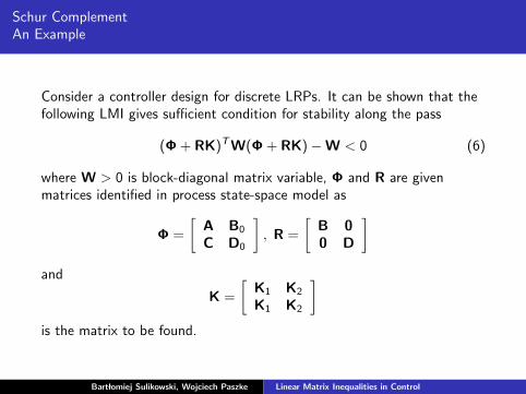
Schur ComplementAn Example

Consider a controller design for discrete LRPs. It can be shown that thefollowing LMI gives sufficient condition for stability along the pass

(Φ + RK)T W(Φ + RK)−W < 0 (6)

where W > 0 is block-diagonal matrix variable, Φ and R are givenmatrices identified in process state-space model as

Φ =

[A B0

C D0

], R =

[B 00 D

]and

K =

[K1 K2

K1 K2

]is the matrix to be found.


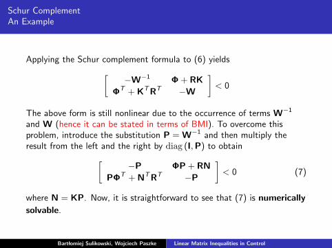
Schur ComplementAn Example

Applying the Schur complement formula to (6) yields[−W−1 Φ + RK

ΦT + KT RT −W

]< 0

The above form is still nonlinear due to the occurrence of terms W−1

and W (hence it can be stated in terms of BMI). To overcome thisproblem, introduce the substitution P = W−1 and then multiply theresult from the left and the right by diag (I, P) to obtain[

−P ΦP + RN

PΦT + NT RT −P

]< 0 (7)

where N = KP. Now, it is straightforward to see that (7) is numerically

solvable.


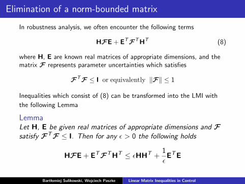
Elimination of a norm-bounded matrix

In robustness analysis, we often encounter the following terms

HFE + ETFT HT (8)

where H, E are known real matrices of appropriate dimensions, and thematrix F represents parameter uncertainties which satisfies

FTF ≤ I or equivalently ‖F‖ ≤ 1

Inequalities which consist of (8) can be transformed into the LMI with

the following Lemma

LemmaLet H, E be given real matrices of appropriate dimensions and Fsatisfy FTF ≤ I. Then for any ε > 0 the following holds

HFE + ETFT HT ≤ εHHT +1

εET E


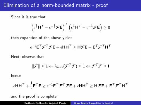
Elimination of a norm-bounded matrix - proof

Since it is true that(ε

12 HT − ε−

12 FE

)T (ε

12 HT − ε−

12 FE

)≥ 0

then expansion of the above yields

ε−1ETFTFE + εHHT ≥ HFE + ETFT HT

Next, observe that

‖F‖ ≤ 1 ⇔ λmax(FTF) ≤ 1 ⇔ FTF ≥ I

hence

εHHT +1

εET E ≥ ε−1ETFTFE + εHHT ≥ HFE + ETFT HT

and the proof is complete.


Elimination of variables

For certain specific matrix inequalities, if is often possible to eliminatesome of the matrix variables.

LemmaLet Ψ ∈ Rq×q be a symmetric matrix and P ∈ Rr×q and Q ∈ Rs×q bereal matrices then there exists a matrix Θ ∈ Rr×s such that

Ψ + PT ΘT Q + QT ΘP < 0

if and only if the inequalities

WTP ΨWP < 0 and WT

QΨWQ < 0

both hold, where WP and WQ are full rank matrices satisfyingIm(WP) = ker(P) and Im(WQ) = ker(Q)

It can also be used to eliminate variables from already formulated LMI.

Since some variables can be eliminated, the computation burden can be

reduced greatly.


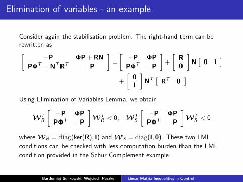
Elimination of variables - an example

Consider again the stabilisation problem. The right-hand term can berewritten as[

−P ΦP + RN

PΦT + NT RT −P

]=

[−P ΦP

PΦT −P

]+

[R0

]N[

0 I]

+

[0I

]NT

[RT 0

]Using Elimination of Variables Lemma, we obtain

WTR

[−P ΦP

PΦT −P

]WT

R < 0, WTS

[−P ΦP

PΦT −P

]WT

S < 0

where WR = diag(ker(R), I) and WS = diag(I, 0). These two LMI

conditions can be checked with less computation burden than the LMI

condition provided in the Schur Complement example.


Illustrative computations have been performed for processes of prescribedorder (n) and the results are listed in the below Table.

Table: Execution time comparison.

n Previous example (CPU time) This example (CPU time)6 0.11 0.068 0.22 0.11

12 1.15 0.615 19.06 1.7620 73.44 7.91

Note that all computations have been performed with Lmi Control

Toolbox 1.0.8 under Matlab 6.5. The Matlab-files have been run

on a PC with AMD Duron 600 MHz CPU and 128MB RAM.


Control problems solved with LMIs - details

I The discrete system state-space equation

xk+1 = Axk + Buk

I Lyapunov inequality for discrete system

AT PA− P < 0, P > 0

I Controller design:The closed loop for the discrete case uk = Kxk (K is thecontroller to be designed)

I The stabilization condition for the discrete case

(A + BK)T P(A + BK)− P < 0, P > 0

not the LMI condition since the variable matrices aremultiplied


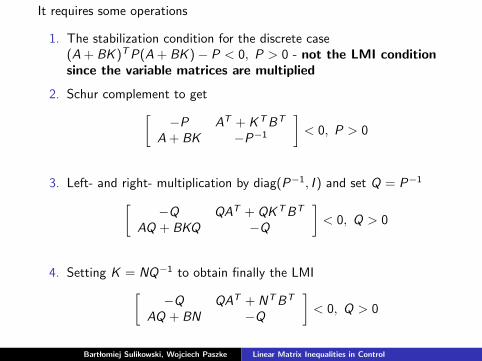
It requires some operations

1. The stabilization condition for the discrete case(A + BK )TP(A + BK )− P < 0, P > 0 - not the LMI conditionsince the variable matrices are multiplied

2. Schur complement to get[−P AT + KTBT

A + BK −P−1

]< 0, P > 0

3. Left- and right- multiplication by diag(P−1, I ) and set Q = P−1[−Q QAT + QKTBT

AQ + BKQ −Q

]< 0, Q > 0

4. Setting K = NQ−1 to obtain finally the LMI[−Q QAT + NTBT

AQ + BN −Q

]< 0, Q > 0


Control problems solved with LMIs - differential case

1D differential system state-space equation x(t) = Ax(t) + Bu(t)Lyapunov inequality for 1D differential system ATP + PA < 0, P > 0Controller designThe closed loop for the different case u(t) = Kx(t)The stabilization condition for the differential case(A + BK )TP + P(A + BK ) < 0, P > 0 - not the LMI condition


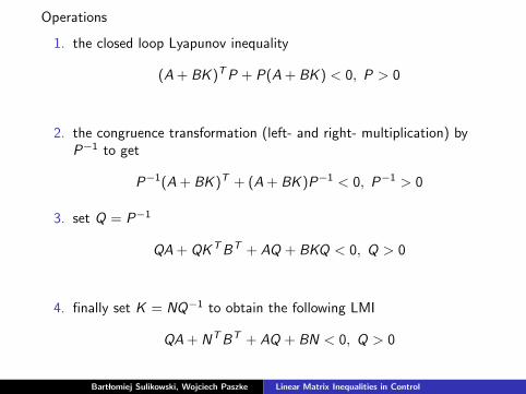
Operations

1. the closed loop Lyapunov inequality

(A + BK )TP + P(A + BK ) < 0, P > 0

2. the congruence transformation (left- and right- multiplication) byP−1 to get

P−1(A + BK )T + (A + BK )P−1 < 0, P−1 > 0

3. set Q = P−1

QA + QKTBT + AQ + BKQ < 0, Q > 0

4. finally set K = NQ−1 to obtain the following LMI

QA + NTBT + AQ + BN < 0, Q > 0


Standard LMI problems

The LMI software can solve the LMI problems formulated in threedifferent forms:

I feasibility problem,

I linear optimization problem,

I generalized eigenvalue minimization problem.


Feasibility problem

A feasibility problem is defined as follows

DefinitionFind a solution x = (x1, . . . , xn) such that

F(x) > 0 (9)

or determine that the LMI (9) is infeasible.

A typical situation for the feasibility problem is a stability problemwhere one has to decide if a system is stable or not (an LMI isfeasible or not).


Linear objective minimization problem

DefinitionMinimize a linear function cT x (x = (x1, . . . , xn)), where c ∈ Rn is agiven vector, subject to an LMI constraint (9) or determine that theconstraint is infeasible. Thus the problem can be written as

min cT x

subject to F(x) > 0

This problem can appear in the equivalent form of minimizing themaximum eigenvalue of a matrix that depends affinely on the variable x ,subject to an LMI constraint (this is often called EVP)

min λ

subject to λI− F(x) > 0


Generalized eigenvalue problem

The generalized eigenvalue problem (GEVP) allows us to minimize themaximum generalized eigenvalue of a pair of matrices that dependaffinely on the variable x = (x1, . . . , xn). The general form of GEVP isstated as follows

min λ

subject to

A(x) < λB(x)

B(x) > 0

C(x) < D(x)

(10)

where C(x) < D(x) and A(x) < λB(x) denote set of LMIs. It isnecessary to distinguish between the standard LMI constraint, i.e.

C(x) < D(x)

and the LMI involving λ (called the linear-fractional LMI constraint)

A(x) < λB(x)

which is quasi-convex with respect to the parameters x and λ. However,

this problem can be solved by similar techniques as those for previous

problems.Bart lomiej Sulikowski, Wojciech Paszke Linear Matrix Inequalities in Control

The stability margins

A system matrix A has a stability margin q, iff the stabilitycondition holds for (1 + q)A.

So, it is straightforward to get the LMI conditions to check if Ahas a’priori defined q. It is also easy to write the appropriatecondition for computing the controller K providing the required qin the closed loop.


In our case (1D discrete case considered) we have the followingLMI condition[

−Q (1 + q)(QAT + NTBT )(1 + q)(AQ + BN) −Q

]< 0, Q > 0

K = NQ−1

RemarkNote that (1 + q) is a scalar, so for any matrix, say T, holds(1 + q)T = T(1 + q)

To get the GEVP condition, the follow the steps (on the next slide)


I [−Q QAT + NT BT

AQ + BN −Q

]<q(−1×

[0 QAT + NT BT

AQ + BN 0

]), Q > 0

I multiply it by q−1 (positive since q > 0) and set λ = q−1 and thenby −1 to obtain[

0 QAT + NT BT

AQ + BN 0

]<λ

[Q −QAT − NT BT

−AQ − BN Q

], Q > 0

I

I write it as the GEVP

min λ s.t.

[0 QAT + NT BT

AQ + BN 0

]<λ

[Q −QAT − NT BT

−AQ − BN Q

][

−Q QAT + NT BT

AQ + BN −Q

]< 0

I K = NQ−1, q = λ−1

I note that the additional constraint is just the stability condition inthis case


D-stability (Poles placement)

References

I LMI MATLAB Control toolbox manual

I M. Chilali and P. Gahinet, “H∞ design with pole placementconstraints: an LMI approach,” IEEE Transactions onAutomatic Control, vol. 41, no. 3, pp. 358–367, 1996.

I M. Chilali, P. Gahinet, and P. Apkarian, “Robust poleplacement in LMI regions,” IEEE Transactions on AutomaticControl, vol. 44, no. 12, pp. 2257–2270, 1999.

I D. Henrion, M. Sebek, and V. Kucera, “Robust poleplacement for second-order systems: an lmi approach,”Proceedings of the IFAC Symposium on Robust ControlDesign, 2003. LAAS-CNRS Research Report No. 02324, July2002, Submitted to Kybernetika, October 2003.

I others


LMI region is any subset D of the complex plane that can be defined as

D = {z ∈ C : L + zM + zMT < 0} (%)

where L and M are real matrices and L = LT

The matrix-valued function

fD(z) = L + zM + zMT

is called the characteristic function of D


A real matrix A is D-stable, i.e. has all eigenvalues inside the D region iffthere exists a symmetric matrix X > 0 such that the following LMI holds

L⊗ X + M ⊗ (XA) + MT ⊗ (ATM) < 0 ($)

where ⊗ denotes the Kronecker product

Very important result !!! - indeed, this generalizes all we said about

the stability


Common known D regions

I half-plane Re(z) < −α : z + z + 2α < 0

I special case of the above i.e. Re(z) < 0 : z + z < 0 - the stabilityregion for the differential system described by A

I disc centered at (−q, 0) with radius r[−r q + z

q + z − r

]< 0

I ellipse centered at (−q, 0) with radiuses a-horizontal and b-vertical[−2a −2g + (1 + a/b)z + (1− a/b)z

−2g + (1− a/b)z + (1 + a/b)z −2a

]=

[−2a −2g−2g −2a

]+ z

[0 (1 + a/b)

(1− a/b) 0

]+ z

[0 (1− a/b)

(1 + a/b) 0

]= L + zM + zMT < 0

I conic sector with apex at the origin and inner angle (see reference)

I any intersection(s) of the above


Application in control

Note, that it is now easy to find the LMI condition which checks, ifmatrix eigenvalues lay inside chosen region - weak? Yes, but ...Instead of A write it in the closed loop configuration i.e. A + BK - weget the way to drive A to have eigenvalues inside chosen region usingcontroller K- strong enough!So, the procedure is as follows

I choose DI write it as LMI region (%)

I write ($)

I use some linear algebra operations to get programmable LMI

I solve it using your favorite software


D-stabilization - example

1. choose ellipse[−2a −2g−2g −2a

]+ z

[0 (1 + a/b)

(1− a/b) 0

]+ z

[0 (1− a/b)

(1 + a/b) 0

]= L + zM + zMT < 0

2. set A = A + BK

3. condition for the closed loop system

L⊗ X + M ⊗ (XA) + MT ⊗ (ATX ) < 0

which can be rewritten as[−2aX (∗)

−2gX + (1 + ab )ATX + (1− a

b )XA −2aX

]< 0

4. set A = A + BK to obtain[−2aX (∗)

−2gX + (1 + ab )(A + BK )TX + (1− a

b )X (A + BK ) −2aX

]< 0

not LMI - again X and K multipliedBart lomiej Sulikowski, Wojciech Paszke Linear Matrix Inequalities in Control

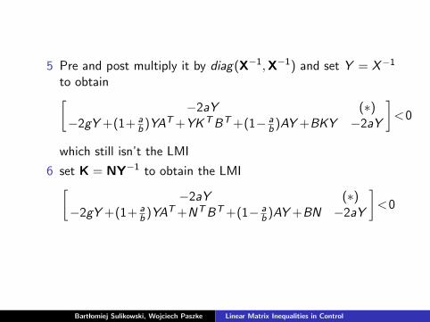
5 Pre and post multiply it by diag(X−1, X−1) and set Y = X−1

to obtain[−2aY (∗)

−2gY +(1+ ab )YAT +YKTBT +(1− a

b )AY +BKY −2aY

]<0

which still isn’t the LMI

6 set K = NY−1 to obtain the LMI[−2aY (∗)

−2gY +(1+ ab )YAT +NTBT +(1− a

b )AY +BN −2aY

]<0


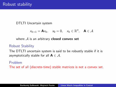
Robust stability

DTLTI Uncertain system

xk+1 = Axk , x0 = 0, xk ∈ Rn, A ∈ A

where A is an arbitrary closed convex set

Robust Stability

The DTLTI uncertain system is said to be robustly stable if it isasymptotically stable for all A ∈ A.

ProblemThe set of all (discrete-time) stable matrices is not a convex set.


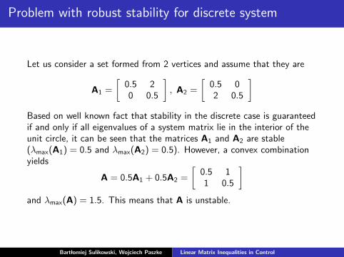
Problem with robust stability for discrete system

Let us consider a set formed from 2 vertices and assume that they are

A1 =

[0.5 20 0.5

], A2 =

[0.5 02 0.5

]Based on well known fact that stability in the discrete case is guaranteedif and only if all eigenvalues of a system matrix lie in the interior of theunit circle, it can be seen that the matrices A1 and A2 are stable(λmax(A1) = 0.5 and λmax(A2) = 0.5). However, a convex combinationyields

A = 0.5A1 + 0.5A2 =

[0.5 11 0.5

]and λmax(A) = 1.5. This means that A is unstable.


Uncertainty

Two main models of uncertainty

I norm-bounded

I polytopic

I affine


Norm-bounded model of uncertainty.

This model of uncertainty corresponds to a system which matricesuncertainty are modelled as an additive perturbation to thenominal system matrices. Therefore a system is said to besubjected to norm-bounded parameter uncertainty if matrices ofsuch a system can be written in the form

M = M0 + ∆M = M0 + HFE

where H and E are some known constant matrices with compatibledimensions and M0 defines the nominal system. F is an unknown,constant matrix which satisfies

FTF ≤ I


Important: The inequality

FTF ≤ I

represents a convex set. To see this, apply the Schur complementformula to obtain

FTF ≤ I ⇔[

I FFT I

]≥ 0


Polytopic model of uncertainty

This model of uncertainty corresponds to a system which matricesrange in the polytope of matrices. This means that each systemmatrix M is only known to lie in a given fix polytope of matricesdescribed by

M ∈ Co (M1, M2, . . . , Mh)

where Co denotes the convex hull. Then, for positivei = 1, 2, . . . , h, M can be written as

M :=

{X : X =

h∑i=1

αiMi , αi ≥ 0,

h∑i=1

αi = 1

}


Polytopic model of uncertainty

As a simple example, the polytope formed from 4 vertices:M1, M2, M3 and M4 is depicted below

M1M

2

M3

M4

Figure: A polytope


Affine model of uncertainty

This model of uncertainty corresponds to a system which matrices aremodelled as a collection of fixed affine functions of some varyingparameters p1, . . . , pk i.e. each matrix can be written in the form

M(p) = M0 + p1M1 + . . . + pkMk (11)

where Mi ∀i = 0, 1, . . . , k are given. Parameter uncertainty is describedwith range of parameter values. It means that each parameter pi rangesbetween two known extremal values pi (minimum) and pi (maximum),therefore it can be written as

pi ≤ pi ≤ pi

Furthermore, the set of uncertain parameters is

∆ ,{p =(p1, p2, . . . , pk) : pi ≤ pi ≤ pi , i =1, . . . , k

}and the set of corners of uncertainty region ∆0 is defined as

∆0 ,{p =(p1, p2, . . . , pk) : p ∈ {pi , pi}, i =1, . . . , k

}Bart lomiej Sulikowski, Wojciech Paszke Linear Matrix Inequalities in Control

Affine model of uncertainty

As an example of a set of uncertain parameters, consider 3parameters: p1, p2, p3 whose values range in the parameter boxformed by their extremal values in 3-D parameter space

p2

p3

p2

p3

p2p3

p1

p1

p1

Figure: 3-D parameter space


Form affine parameter-dependent matrices to the polytopicform

It is clear that M(p) is an affine function in p = (p1, p2, . . . , pk),thus it maps these corners to the polytope of vertices. In this caseeach vertex can be determined ∀p ∈ ∆0 with the formula below

Mi = M0 + p1M1 + . . . + pkMk

where i = 1, .., 2k .

p1

p1

p1

p2p2p2

M1

M2

M4

M3

Figure: Transformation from the affine model to the polytopic modelBart lomiej Sulikowski, Wojciech Paszke Linear Matrix Inequalities in Control

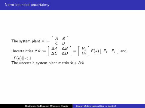
Norm-bounded uncertainty

The system plant Φ :=

[A BC D

]Uncertainties ∆Φ :=

[∆A ∆B∆C ∆D

]=

[H1

H2

]F (k)

[E1 E2

]and

||F (k)|| < 1The uncertain system plant matrix Φ + ∆Φ


Norm-bounded uncertainty

Discrete case - controller design (so we want to get the condition for computing K)

I For simplicity take F (k) = F - no loose of generalization

I The Lyapunov inequality for the closed loop uncertain system

(A + H1FE1 + BK + H1FE2K)T P(A + H1FE1 + BK + H1FE2K)−P < 0, P > 0

I Schur complement[−P AT + ET

1 FT HT1 + KT BT + KT ET

2 FT HT1

A + H1FE1 + BK + H1FE2K −P−1

]< 0, P > 0

I write it as[−P AT + KT BT

A + BK −P−1

]+

[0 ET

1 FT HT1 + KT ET

2 FT HT1

H1FE1 + H1FE2K 0

]< 0, P > 0


I or[−P AT + KT BT

A + BK −P−1

]+

[ET

1 + KT ET2

0

] [FT

] [0 HT

1

]+

[0H1

] [F

] [E1 + E2K 0

]< 0, P > 0

I apply Lemma 2 to obtain[−P AT + KT BT

A + BK −P−1

]+ ε−1

[ET

1 + KT ET2

0

] [E1 + E2K 0

]+ε

[0H1

] [0 HT

1

]< 0, P > 0, ε > 0


I write it as (since ε is a scalar)[−P AT + KT BT

A + BK −P−1

]+

[ET

1 + KT ET2

εH1

] [ε−1I

] [E1 + E2K εHT

1

]< 0, P > 0, ε > 0

I Apply the Schur complement again −P AT + KT BT ET1 + KT ET

2A + BK −P−1 εH1

E1 + E2K εHT1 −εI

< 0, P > 0, ε > 0

still not the LMI

I congruence by diag(P−1, I , I ) and set Q = P−1

−Q QAT + QKT BT QET1 + QKT ET

2AQ + BKQ −Q εH1

E1Q + E2KQ εHT1 −εI

< 0, Q > 0, ε > 0

I finally set K = NQ−1 to obtain the LMI −Q QAT + NT BT QET1 + NT ET

2AQ + BN −Q εH1

E1Q + E2N εHT1 −εI

< 0, Q > 0, ε > 0


Thank you very much for your attention


Linear Matrix Inequalities in Controlstaff.uz.zgora.pl/wpaszke/materialy/ts/slides_1print.pdf ·...

Documents

Transcript of Linear Matrix Inequalities in Controlstaff.uz.zgora.pl/wpaszke/materialy/ts/slides_1print.pdf ·...