Linear Inequalities and Linear Programming Chapter 5 Dr.Hayk Melikyan/ Department of Mathematics and...
23
Linear Inequalities and Linear Programming Chapter 5 Dr .Hayk Melikyan/ Department of Mathematics and CS/ [email protected] Linear Programming in two dimensions: a geometric approach In this section, we will explore applications which utilize the graph of a system of linear inequalities.
-
Upload
nick-barner -
Category
Documents
-
view
221 -
download
1
Transcript of Linear Inequalities and Linear Programming Chapter 5 Dr.Hayk Melikyan/ Department of Mathematics and...

Linear Inequalitiesand Linear Programming
Chapter 5
Dr .Hayk Melikyan/ Department of Mathematics and CS/ [email protected]
Linear Programming in two dimensions: a geometric approach
In this section, we will explore applications which utilize the graph of a system of linear inequalities.

FM/04/Melikyan
A familiar example
We have seen this problem before. An extra condition will be addedto make the example more interesting. Suppose a manufacturermakes two types of skis: a trick ski and a slalom ski. Suppose eachtrick ski requires 8 hours of design work and 4 hours of finishing.Each slalom ski 8 hours of design and 12 hours of finishing.Furthermore, the total number of hours allocated for design work is160 and the total available hours for finishing work is 180 hours. Finally, the number of trick skis produced must be less than or equalto 15. How many trick skis and how many slalom skis can be madeunder these conditions? Now, here is the twist: Suppose the profit on each trick ski is $5 andthe profit for each slalom ski is $10. How many each of each type ofski should the manufacturer produce to earn the greatest profit?

FM/04/Melikyan
Linear Programming problem
This is an example of a linear programming problem. Every linear programming problem has two components:
1. A linear objective function is to be maximized or minimized. In our case the objective function is
Profit = 5x + 10y (5 dollars profit for each trick ski manufactured and $10 for every slalom ski produced).
2. A collection of linear inequalities that must be satisfied simultaneously. These are called the constraints of the problem because these inequalities give limitations on the values of x and y. In our case, the linear inequalities
are the constraints.0
0
15
8 8 160
4 12 180
x
y
x
x y
x y
x and y have to be positive
The number of trick skis must be less than or equal to 15
Design constraint: 8 hours to design each trick ski and 8 hours to design each slalom ski. Total design hours must be less than or equal to 160
Finishing constraint: Four hours for each trick ski and 12 hours for each slalom ski.
Profit = 5x + 10y

FM/04/Melikyan
FM/04/Melikyan

FM/04/Melikyan
Linear programming
3. The feasible set is the set of all points that are possible for thesolution. In this case, we want to determine the value(s) of x, thenumber of trick skis and y, the number of slalom skis that will yieldthe maximum profit. Only certain points are eligible. Those are thepoints within the common region of intersection of the graphs of theconstraining inequalities. Let’s return to the graph of the system oflinear inequalities. Notice that the feasible set is the yellow shadedregion. Our task is to maximize the profit function P = 5x + 10y by producing x trick skis and y slalom skis, but use only values of xand y that are within the yellow region graphed in the next slide.

FM/04/Melikyan
FM/04/Melikyan
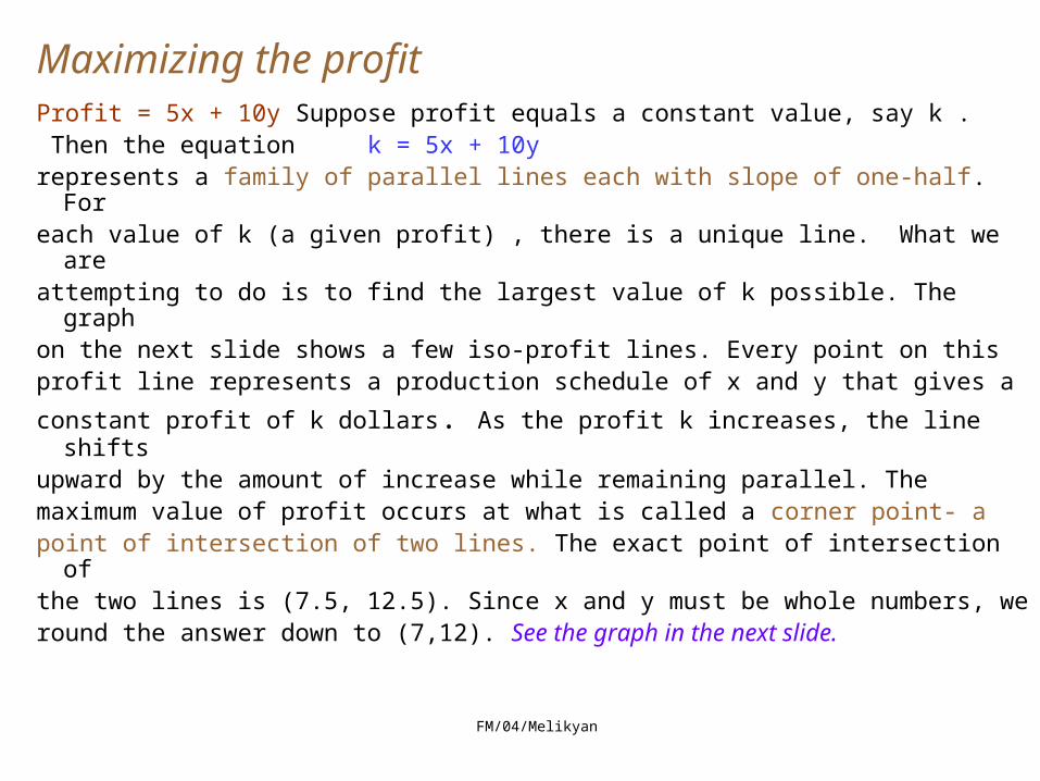
Maximizing the profit
Profit = 5x + 10y Suppose profit equals a constant value, say k . Then the equation k = 5x + 10y represents a family of parallel lines each with slope of one-half. Foreach value of k (a given profit) , there is a unique line. What we areattempting to do is to find the largest value of k possible. The graphon the next slide shows a few iso-profit lines. Every point on thisprofit line represents a production schedule of x and y that gives a
constant profit of k dollars. As the profit k increases, the line shifts
upward by the amount of increase while remaining parallel. Themaximum value of profit occurs at what is called a corner point- apoint of intersection of two lines. The exact point of intersection ofthe two lines is (7.5, 12.5). Since x and y must be whole numbers, weround the answer down to (7,12). See the graph in the next slide.

FM/04/Melikyan

FM/04/Melikyan
Maximizing the Profit
Thus, the manufacturer should produce 7 trick skis and 12 slalom
skis to achieve maximum profit. What is the maximum profit?
P = 5x + 10y
P=5(7)+10(12)=35 + 120 = 155

FM/04/Melikyan
General Result
If a linear programming problem has a solution, it is located at avertex of the set of feasible solutions. If a linear programmingproblem has more than one solution, at least one of them is located ata vertex of the set of feasible solutions.
If the set of feasible solutions is bounded, as in our example, then itcan be enclosed within a circle of a given radius. In these cases, thesolutions of the linear programming problems will be unique.
If the set of feasible solutions is not bounded, then the solution mayor may not exist. Use the graph to determine whether a solutionexists or not.

FM/04/Melikyan
General Procedure for Solving Linear Programming Problems
1. Write an expression for the quantity that is to be maximized or minimized. This quantity is called the objective function and will be of the form z = Ax + By. In our case z = 5x + 10y.
2. Determine all the constraints and graph them
3. Determine the feasible set of solutions- the set of points which satisfy all the constraints simultaneously.
4. Determine the vertices of the feasible set. Each vertex will correspond to the point of intersection of two linear equations. So, to determine all the vertices, find these points of intersection.
5. Determine the value of the objective function at each vertex.

FM/04/Melikyan
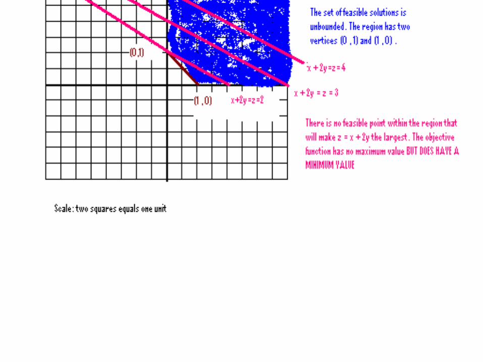
Linear programming problem with no solution
Maximize the quantity z =x +2y subject to the constraints x + y 1 , x 0 , y 0
1. The objective function is z = x + 2y is to be maximized.
2. Graph the constraints: (see next slide)
3. Determine the feasible set (see next slide)
4. Determine the vertices of the feasible set. There are two vertices from our graph. (1,0) and (0,1)
5. Determine the value of the objective function at each vertex.
6. at (1,0): z = (1) + 2(0) = 1 at (0, 1) : z = 0 + 2(1) = 2 .
We can see from the graph there is no feasible point that makes z largest. Weconclude that the linear programming problem has no solution.
FM/04/Melikyan

FM/04/Melikyan
LINEAR PROGRAMMING PROBLEM
is a problem concerned with finding the maximum or minimumvalue of a linear OBJECTIVE FUNCTION of the form
z = c1x1 + c2x2 + ... + cnxn,
where the DECISION VARIABLES x1, x2, ..., xn are subject toPROBLEM CONSTRAINTS in the form of linear inequalities andequations. In addition, the decision variables must satisfy theNONNEGATIVE CONSTRAINTS
xi ≥ 0, for i = 1, 2, ..., n. The set of points satisfying both the problem constraints and thenonnegative constraints is called the FEASIBLE REGION for theproblem. Any point in the feasible region that produces theoptimal value of the objective function over the feasible region iscalled an OPTIMAL SOLUTION.

FM/04/Melikyan
CONSTRUCTING THE MATHEMATICAL MODEL
For the applied Linear programming problem
1. Introduce decision variables
2 Summarize relevant material in table form, relating the
decision variables with the columns in the table, if possible.
3. Determine the objective and write a linear objective function.
4. Write problem constraints using linear equations and/or inequalities.
5. Write non-negative constraints.

FM/04/Melikyan
FUNDAMENTAL THEOREM OF LINEAR PROGRAMMING
If the optimal value of the objective function in a linear
programming problem exists, then that value must
occur at one (or more) of the corner points of the
feasible region

FM/04/Melikyan
EXISTENCE OF SOLUTIONS
(A) If the feasible region for a linear programming problem is bounded, then both the maximum value and the minimum value of the objective function always exist.
(B) If the feasible region is unbounded, and the coefficients of the objective function are positive, then the minimum value of the objective function exists, but the maximum value does not.
(C) If the feasible region is empty (that is, there are no points that satisfy all the constraints), the both the maximum value and the minimum value of the objective function do not exist.
FM/04/Melikyan
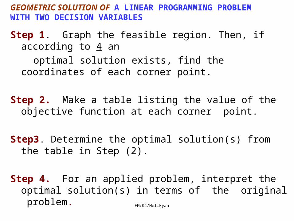
GEOMETRIC SOLUTION OF A LINEAR PROGRAMMING PROBLEM WITH TWO DECISION VARIABLES
Step 1. Graph the feasible region. Then, if according to 4 an
optimal solution exists, find the coordinates of each corner point.
Step 2. Make a table listing the value of the objective function at each corner point.
Step3. Determine the optimal solution(s) from the table in Step (2).
Step 4. For an applied problem, interpret the optimal solution(s) in terms of the original problem.
FM/04/Melikyan
Example (33)
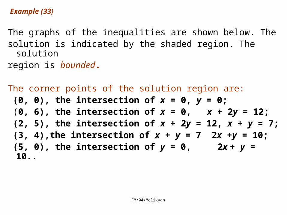
The graphs of the inequalities are shown below. Thesolution is indicated by the shaded region. The solutionregion is bounded.
The corner points of the solution region are: (0, 0), the intersection of x = 0, y = 0; (0, 6), the intersection of x = 0, x + 2y = 12; (2, 5), the intersection of x + 2y = 12, x + y = 7; (3, 4),the intersection of x + y = 7 2x +y = 10; (5, 0), the intersection of y = 0, 2x + y = 10..

FM/04/Melikyan
Graph of example (33)
2x + y = 10
x + 2y = 12
x + y = 7
Bounded
(2, 5)(0, 6)
(5, 0)(0, 0)

FM/04/Melikyan
Example( Problem # 21 Chapter 5.2)
Step (1): Graph the feasible region and find the corner points. The feasible region S is the solution set of the given inequalities, and is indicated by the shading in the graph at the right. The corner points are (3, 8), (8, 10), and (12, 2). Since S is bounded, it follows that P has a maximum value and a minimum value.
x2
x1
Bounded
(8, 10)
(3, 8)
(12, 2)
-2 x1 + 5x2 = 34
2x1 + x2 = 26
1 22x + 3x = 30

FM/04/Melikyan
x2
x1
Bounded
(8, 10)
(3, 8)
(12, 2)
-2 x1 + 5x2 = 34
2x1 + x2 = 26
1 22x + 3x = 30

FM/04/Melikyan
Example ( continue)
Step (2): Evaluate the objective function at each corner point. the value of P at each corner point is
(3, 8) P = 20(3) + 10(8) = 140
(8, 10) P = 20(8) + 10(10) = 260 (12, 2) P = 20(12) + 10(2) = 260
Step (3): Determine the optimal solutions.
The minimum occurs at x1 =3, x2 = 8, and the minimum value is P =140;
the maximum occurs at x1 = 8, x2 = 10, at x1 = 12, x2 = 2, and at any point along the line segment joining (8, 10) and (12, 2). The maximum value is P = 260.