Linear and Ultrasound Measurements in Crossbred Goats … · Linear and Ultrasound Measurements in...

Linear and Ultrasound Measurements in Crossbred Goats as a Predictor of Live and Hot Carcass Weights

Submitted to the University of Tennessee at Martin In partial fulfillment of requirements

For the degree of

Master of Science

Agriculture and Natural Resources Systems Management

Nathan Stamper

August 2010

ii

Abstract

This study was conducted to examine correlations between live linear and real‐time

ultrasound measurements and carcass characteristics in Spanish x Boer goats. Goats

were housed at the University of Tennessee‐Martin Sheep and Goat Research and

Teaching Farm and grazed on pasture in late summer and fall, 2008. Body weight,

ultrasound and linear measurements were recorded three times during the study. Body

weight (BW) was determined using a Gallagher scale. Ultrasound measurements

included: body wall thickness (BWT), hide thickness (HT), fat layer thickness (FLT) and

Loin Depth (LD). Linear measurements included: cannon length (CL), cannon

circumference (CC), shoulder height (SH), heart girth (HG), last rib girth (LR), and

circumference of neck (NECK). Goats were transported to Meacham Packing Company

(Batesville, AR) and were kosher slaughtered by exsanguination under the inspection of

the United States Department of Agriculture. Immediately following slaughter, hot

carcass weight (HCW) was recorded. Pearson correlation coefficients were calculated

using Proc Corr in SAS; Proc Reg was used to determine regression equations for

predicting BW and HCW. Regression using linear measurements and ultrasonography as

input variables produced models to predict BW and HCW with R2 values of 0.73 and

0.38, respectively. The data suggest that reasonable predictions of BW can be made

using only linear measurements, especially CC, SH and LR. This finding is important for

small goat producers who lack resources to purchase and maintain digital scales and

ultrasound equipment.

iii

Table of Contents

Introduction .................................................................................................................... 1

Objectives ............................................................................................................ 2

Literature Review ............................................................................................................ 3

History of Goats .................................................................................................. 3

National and State Goat Statistics ...................................................................... 4

Meat Goat Production ........................................................................................ 5

Use of Weights .................................................................................................... 6

Predicting Body Weight Using Linear Measurements ........................................ 7

Materials and Methods ................................................................................................... 9

Animals ................................................................................................................. 9

Data Collection ................................................................................................... 10

Data Analysis ...................................................................................................... 10

Results ........................................................................................................................... 12

Linear Measurements ........................................................................................ 12

Ultrasound Measurements ................................................................................ 17

Discussion ...................................................................................................................... 19

Conclusion ..................................................................................................................... 21

Works Cited ................................................................................................................... 26

Appendix ....................................................................................................................... 27

iv

List of Tables

Table 1: Correlations among body weight (BW), cannon length (CL), cannon circumference (CC), shoulder height (SH), heart girth(HG), girth at the last rib (LR), neck girth (NECK) and hot carcass weight (HCW) of goats measured on Date 1. ................ 23

Table 2: Correlations among body weight (BW), cannon length (CL), cannon circumference (CC), shoulder height (SH), heart girth(HG), girth at the last rib (LR), neck girth (NECK) and hot carcass weight (HCW) of goats measured on Date 2. ................ 23

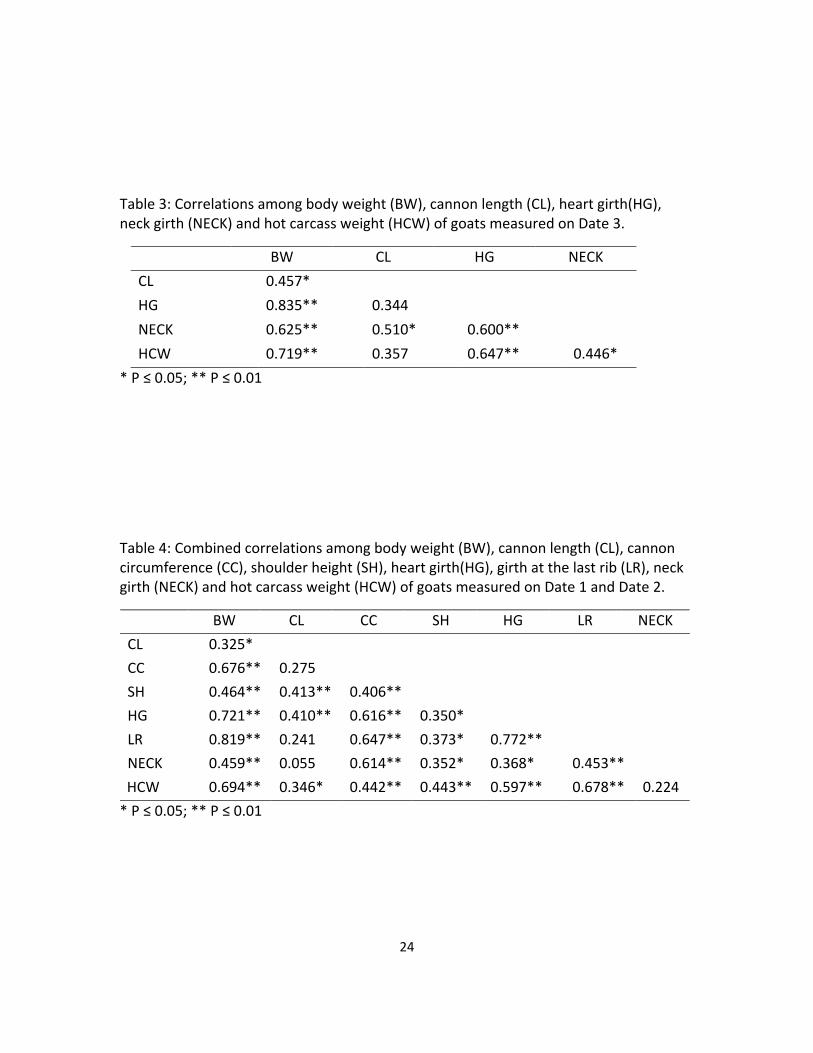
Table 3: Correlations among body weight (BW), cannon length (CL), heart girth (HG), neck girth (NECK) and hot carcass weight (HCW) of goats measured on Date 3. ........ 24

Table 4: Combined correlations among body weight (BW), cannon length (CL), cannon circumference (CC), shoulder height (SH), heart girth (HG), girth at the last rib (LR), neck girth (NECK) and hot carcass weight (HCW) of goats measured on Date 1 and Date 2. ................................................................................................... 24

Table 5: Combined correlations among body weight (BW), cannon length (CL), heart girth (HG), neck girth (NECK) and hot carcass weight (HCW) of goats measured on Date 1, Date 2, and Date 3. ...................................................................................... 25

Table 6: Combined correlations among body weight (BW), cannon length (CL), heart girth (HG), neck girth (NECK), hide thickness (HT), fat thickness (FT), loin depth (LD), body wall thickness (BWT), and hot carcass weight (HCW) of goats measured on Date 1, Date 2, and Date 3. ...................................................................................... 25

Table A.1: Stepwise Regression for BW Using Linear Measurements from Date 1 and Date 2 ............................................................................................................................ 27

Table A.2: Stepwise Regression for HCW Using Linear Measurements from Date 1 and Date 2 ......................................................................................................... 27

Table A.3: Stepwise Regression for BW Using Three Linear Measurements from Date 1, Date 2, and Date 3. ........................................................................................... 27

Table A.4: Stepwise Regression for HCW Using Three Linear Measurements from Date 1, Date 2, and Date 3. ........................................................................................... 27

Table A.5: Stepwise Regression for BW Using Linear and Ultrasound Measurements .............................................................................................................. 28

Table A.6: Stepwise Regression for HCW Using Linear and Ultrasound Measurements .............................................................................................................. 28

1

Introduction Livestock operations in Tennessee and the Southeast are typically operated as

part‐time entities that provide supplemental income to the producer. Goats are

commonly found on such farms, especially in Tennessee, which is the second largest

goat producing state in the U.S. (NASS, 2007). Compared with cattle, goats have a

greater stocking rate, do not require additional feed inputs, may be sustained on low

quality forages, and can browse weeds, saplings and overly mature plants. Additionally,

the demand for chevon, or goat meat, has greatly increased over the past several years

in the U.S. This is due, in some part, to cultural diversification, especially on both the

east and west coasts. Therefore, due to lower production inputs compared to cattle,

increased demand for chevon, and Tennessee’s proximity to the east coast market, the

goat population in Tennessee has flourished. This gives part‐time producers an

additional source of diversified income for their farms.

In any livestock operation, body weight (BW) is a crucial piece of information

that a producer needs to know to make proper management decisions. However,

purchasing scales to accurately measure BW can be a costly endeavor for the producer

and many part‐time producers are not willing to make this investment. However,

without an accurate BW, making sound management decisions is daunting, if not

impossible. This is true pertaining to animal health and pharmaceutical administration,

due to: (1) the public’s negative opinion about overuse of antibiotics and (2) the

potential for anthelmintic resistant strains of Haemonchus contortus. The importance of

2

BW is amplified because pharmaceuticals are given on a per pound basis. If the

producer improperly administers antibiotics or de‐wormers, profits may decrease, and

pharmaceutical resistance in certain microorganisms may be accelerated.

In the past, goat research has been a low priority in the U.S. compared with

cattle, swine, and sheep. Most research conducted on goats has occurred in countries

such as India, where chevon and goat dairy products are commonly consumed.

Objectives

The objective of this research project was to develop a predictive formula for

body weight (BW) and hot carcass weight (HCW) based on correlations and stepwise

regressions from linear and/or ultrasound measurements on Spanish x Boer goats.

3

Literature Review

History of Goats

Goats were one of the earliest animals to be domesticated. Many experts argue

whether the sheep or the goat was domesticated first. The domestication of both

species has been traced back to long before the writings of the New Testament. Most

scholars agree that domestication for both sheep and goats occurred at about the same

time, because archeological sites dating back to 7,000 B. C. contained remains of both

species (Ensminger, 2002).

The human race has relied on goats since their domestication and their utility

has proved to be indispensable. Goats gave early man meat, fiber, cloth, shelter, tools,

and milk. The meat of the animal was used for food, while fiber and leather from goat

hides were used for clothing and shelter. Even after the development of more

permanent housing, the goat has still maintained its place in many cultures. Its milk was

consumed by man and animal alike, and was used to make cheese and other dairy

products. Older does and bucks were slaughtered for their meat, called chevon,

normally after they had served in these other useful ways. Over time, dual‐purpose goat

breeds were developed to provide adequate amounts of milk as well as high quality

meat.

Today, goats are found in small numbers on many farms. Due to their browsing

habits, goats are often used to keep land clear of brush and weeds. There is a niche

4

market for dairy products from goats, as it is used to make many different cheeses.

Worldwide, more people drink and consume dairy products from goats than from cattle

(Belanger, 1974). Chevon is not readily consumed in the U.S., but as cultural markets

have opened up and expanded, the demand for chevon has increased.

National and State Goat Statistics

According to the USDA’s Agriculture Census (NASS, 2007), there were nearly

150,000 farms with goats and just over 3.1 million goats in the U.S. in 2007. This equates

to an average of 20.6 goats per farm. These numbers have increased from 2002, when

there were 91,000 farms with goats and 2.5 million goats in the U.S. (NASS, 2002). Texas

has the largest number of goats with over 1.1 million head. Tennessee, Oklahoma, and

California are the states with the next largest goat populations, totaling over 100,000

goats (NASS, 2007).

The USDA Agriculture Census divides the U. S. goat population into three

segments: dairy, angora, and meat. Currently about 350,000 dairy goats are found on

27,000 farms in the U.S. California leads the country in dairy goat production with

39,000 dairy goats. The number of angora goats, which produce mohair fiber, has

decreased since the 2002 census from 300,000 to 200,000. Production of mohair has

decreased to about 1.4 million pounds because the U.S. lacks the infrastructure to

process the mohair fiber. Most fiber is exported for processing and then imported as a

finished product. Texas leads the U.S. with 130,000 angora goats producing nearly one

5

million pounds of mohair. Meat type goats make up about 84% of the national goat

population with over 2.6 million head. This figure has increased by over a half a million

head since last documented in 2002. Texas has a meat goat population of nearly one

million animals followed by Tennessee and Oklahoma with over 100,000 head each

(NASS, 2007).

According to NASS (2007), Tennessee has an overall goat population of

approximately 131,000 head, on 7,000 farms. This equates to an average of 18.7 goats

per farm. The state ranks as the second highest in total goat numbers in the country.

Tennessee ranks as the nineteenth state in the U.S. for number of dairy goats with

roughly 6,000 goats, and thirty‐seventh for number of Angora goats with only 250 head

producing 1,100 pounds of mohair annually. In meat goat production, however, the

state ranked second with 125,000 meat goats that produced revenue of 6.7 million

dollars in 2007.

Meat Goat Production

Meat goat production, as in other species, begins with the breeding season. The

crossbred goats that are used for meat production are not seasonal breeders like some

purebred goats. The gestation period of a goat is about five months (Ensminger, 2002),

which allows for two breeding seasons per year, thus conceivably doubling the

producer’s annual output. While mature animals may be sold for consumption, most

goat meat comes from kids. These animals are normally sold at an age of four to five

6

months. This age coincides with the weaning age of the kids. When marketing kids, the

producer, typically chooses from three options: (1) sell their animals through a sale

barn, (2) sell the meat directly to the consumer, but the animal has to be slaughtered at

a USDA inspected facility, or (3) sell animals directly from the farm for individual

slaughter. However, to get the best price, using a barn that regularly has goat sales is

preferred.

Use of Weights

The body weight (BW) of goats represents an important piece of information

that is needed to manage the stock properly. Unfortunately, livestock scales are quite

expensive and not economically feasible for small producers. However, if producers

could estimate BW it would allow them to provide adequate nutrition, correctly

administer medication and better estimate potential profit. For instance, most

medication and de‐wormers are given on a per‐unit of BW basis and either a sub

therapeutic dose or an overdose, can be harmful to the animal and greatly affect

profitability. The BW is also important nutritionally, especially in breeding stock, as the

producer usually makes feeding decisions based on percent of BW. Knowing the

approximate BW of goats, therefore, would allow the producer to make more sound

management decisions.

7

Predicting Body Weight Using Linear Measurements

Ensminger (2002), developed a BW equation where the heart girth is squared,

multiplied by body length and then divided by 300. Three studies, conducted outside

the U.S., have examined the relationships between linear measurements and the

prediction of BW.

Attah et al. (2004) looked at two goat breeds found in West Africa, the Red

Sokoto and West African Dwarf. They wanted to determine if animals slaughtered at a

predetermined BW had similar body measurements. In their research, they used bucks

and does from each breed. The animals were slaughtered at 10, 15, or 20 kilograms.

Seventeen measurements were taken on each goat both pre‐ and post‐slaughter. The

live measurements included: height at withers, height at pelvis, width at pelvis, depth of

chest, chest girth, width of chest, and carcass length. For Red Sokoto goats, there were

no significant differences among slaughter weights for height at the withers, depth of

chest, or carcass length. For the other measurements, at least two of the slaughter

weights had means that were not significantly different. The West African dwarf goats

had similar means for the larger two slaughter weights in every measurement except

the width of pelvis. The researchers cite the small frame of the dwarf goat as the cause

of the discrepancy in the means at the smaller slaughter weight versus those in the

larger two. The researchers also compared males to females and found that few of the

means were similar. Chest girth and width of chest were significantly correlated to

8

dressing percentage at all three slaughter weights. No body measurements had similar

correlation coefficients across all three slaughter weights.

In another study, 122 Black Bengal wethers were subdivided into three groups

based on their locations in Bangladesh (Rahman, 2007). Group A had significant

correlations between live weight and each of heart girth, body length, and wither

height. Group B had significant correlations between the live weight and body length,

wither height, heart girth, rib‐saddle joint length, and hip width. Only BW and HCW

were correlated (P < 0.1) in Group C. Rahman, used these correlated measurements, to

develop several models for the prediction of live weight.

The third study conducted by Thiruvenkadan and Panneerselvamused (2009)

used Kanni Adu goats in India. The animals were between one and six years old; 257

were females while the remaining 47 were males. The researchers took four

measurements: body weight, height at withers, chest girth, and body length. All three of

the body measurements were significantly correlated (P < 0.01) with BW.

Linear measurements are used to find the volume, i.e., the height, width, and

length, of the goat, which should be directly related to weight. Now that the

relationships between linear measurements and weight are better understood,

researchers should be able to streamline the number of measurements needed to

predict BW in goats.

9

Materials and Methods

Animals

Twenty‐six male and female Spanish x Boer cross goats were obtained from the

Tennessee Livestock Producer’s sale barn in Columbia, TN. Handling procedures were

done in accordance with UT Martin Agricultural Animal Care and Use Committee. The

animals were placed in a quarantine pen at the University of Tennessee at Martin (UTM)

Teaching Farm. Fecal egg counts were performed by the on‐staff veterinarian, and it was

determined that the animals had a large number of internal parasites that included

hook, round, and tape worms as well as Haemonchus contortus and coccidia. They were

subsequently de‐wormed by oral drench with 11.36% Albendazole (Valbazen; Pfizer

Animal Health) and Moxidectin (Cydectin; Fort Dodge/Pfizer Animal Health), and placed

on amprolium 9.6% (Corrid; Merial) regiment for five days. All de‐wormers were

administered as oral drenches according to the label. During this time, three goats died

from the heavy parasite load, which was confirmed via necropsies at the West

Tennessee Diagnostics Lab (Martin, TN). The animals were then transported to the UTM

Sheep and Goat Research Facility, where the remaining 23 were sorted into four groups

and rotationally grazed on mixed grass pastures. Each group of animals was placed in a

0.2 hectare (0.5 ac) pen. Goats in this research project were fed no supplemental grain

or roughage.

10

Data Collection

On August 18, 2008 all goats were caught and placed in a dry lot for a 12 hour

shrink. The following day (Date 1) they were weighed and linear and ultrasound

measurements were taken with the help of researchers at UTM. Each group of animals

was then moved to a new 0.2 hectare (0.5 ac) paddock. Measurements were obtained

with a Gallagher Scale (130 West 23rd Av. North Kansas City, MO.), an Ultrasound

Scanner (Pie Medical 200 SLC, the Netherlands), and a tailor’s measuring tape.

Ultrasound measurements were taken at the last rib for hide thickness (HT), fat

thickness (FT), body wall thickness (BWT), and depth of loin (LD). The linear

measurements were cannon length (CL), cannon circumference (CC), heart girth (HG),

shoulder height (SH), neck girth (NECK), and girth at the last rib (LR). This procedure was

repeated two weeks later (Date 2). Due to equipment problems, goats were not

measured again for nine weeks. During this time one goat died. The third time (Date 3)

the animals were measured, all ultrasound measurements were taken but only CL, HG,

and NECK were measured. Following data collection, goats were transported to a

Meacham Packing Company (Batesville, AR). After slaughter, the HCW was obtained

from the employees of the packing plant.

Data Analysis

The data were analyzed using Proc Corr and Proc Reg Procedures of SAS.

Correlations and multiple regression were conducted separately for each of the three

11

sampling dates. For the first two sampling events (Date 1 and Date 2), all linear

measurements were combined and analyzed together. The CL, HG, and SH data were

combined for all three data collection dates and analyzed for correlation and regression.

Finally, data on CL, HG, SH and all ultrasound measurements were combined for

analysis. Multiple regression and stepwise regression analysis was used to determine

which linear and ultrasound measurements could be used to predict BW and HCW.

12

Results

Linear Measurements

Linear measurement data were initially analyzed as three individual groups with

HCW included. Subsequently, data from the first sampling event (Date 1) were

combined with data from the second sampling event (Date 2) and analyzed together

(more linear measure categories were taken for Date 1 and Date 2 sampling events). For

the third sampling event (Date 3), CC, LR, and SH linear measures were inadvertently

omitted due to a miscommunication with the sampling team.

For Date 1, five of the six linear measurements were correlated with BW (Table

1). The CC (r = 0.58), HG (r = 0.66), and LR (r = 0.82) were highly correlated (P ≤ 0.01)

with BW. Both CL and SH were also correlated with BW at P ≤ 0.05 (Table 1). Multiple

regression analysis for BW as a function of all six linear measurements yielded the

following equation:

BW = ‐120.65 + (CL*0.02) + (CC*‐1.16) + (SH*0.78) + (HG*0.37) + (LR*1.34) +

(NECK*0.16),

with an R2 = 0.72 and P = 0.0015. (Equation 1)

Stepwise regression analysis yielded a reduced model which included only LR and SH:

13

BW = ‐113.08 + (SH*0.79) + (LR*1.49),

with an R2 = 0.72 and P ≤ 0.0001. (Equation 2)

The R2 value for the reduced model (Equation 2) was almost identical to that of the full

model (Equation 1). Therefore, of the linear measurements recorded on Date 1, LR and

SH account for most of the variation in BW.

When the linear measurements from Date 1 were correlated with HCW of the

animals, only HG (r = 0.59) and LR (r = 0.68) were correlated (P ≤ 0.01) with HCW (Table

1). For both the full model and reduced model (stepwise regression) of HCW as a

function of linear measurements, the R2 values were low at 0.55 and 0.46 respectively.

For Date 2, again five of the six measurements were correlated with BW (Table

2). However, this time four of the measurements were highly correlated (P ≤ 0.01): CC,

SH, HG, and LR. The NECK was also correlated at P ≤ 0.05 (Table 2). Multiple regression

analysis for BW as a function of all six linear measurements yielded the following

equation:

BW = ‐92.27 + (CL*0.32) + (CC*‐0.07) + (SH*0.61) + (HG*0.56) + (LR*0.89) + (NECK*0.09),


Stepwise regression analysis yielded a reduced model that included only SH, HG, and LR:

14

BW = ‐93.42 + (SH*0.67) + (HG*0.58) + (LR*0.90),


The R2 value for the reduced model (Equation 4) was identical to that of the full model

(Equation 3). Therefore, of the linear measurements recorded on Date 2 of this study,

SH, HG, and LR account for most of the variation in BW. The R2 value (0.95) for Equation

4 was higher than that of Equation 2 (R2 = 0.72), the reduced model from Date 1,

possibly because of the inclusion of an additional variable, (HG) in the model.

Correlation analysis for data from Date 2 revealed that, CC (r = 0.50), SH (r =

0.47), and HG (r = 0.61) were correlated (P ≤ 0.05) with HCW (Table 2). Only LR (r = 0.68)

was correlated at P ≤ 0.01. For both the full model and reduced model (stepwise

regression) of HCW as a function of linear measurements, the R2 values were again 0.55

and 0.46, respectively.

Only three linear measurements were taken on data collection Date 3, as

opposed to six measurements on the previous data collection events. Two of the three

measurements were highly correlated (P ≤ 0.01) with BW: NECK (r = 0.62) and

HG (r = 0.83). Cannon length was also correlated (P ≤ 0.05) with BW (Table 3). Multiple

regression analysis for BW as a function of all three linear measurements yielded the

following equation:

15

BW = ‐54.58 + (CL*1.26) + (HG*1.27) + (NECK*0.37),


Stepwise regression analysis yielded a reduced model that included only CL and HG:

BW = ‐53.55 + (CL*1.61) + (HG*1.38),


When the linear measurements from Date 3 were correlated with HCW of the

animals, only NECK (r = 0.45, P ≤ 0.05) and HG (r = 0.65, P ≤ 0.01) were correlated with

HCW (Table 3). For both the full model and reduced model (stepwise regression) of

HCW as a function of linear measurements, the R2 values were low at 0.44 and 0.42,

respectively.

The data from the Date 1 and Date 2 were combined and analyzed together to

increase sample size. Data collected for Date 3 was excluded due to the fewer number

of linear measurements taken. For this combined data set (Date 1 and Date 2), all six

linear measurements were correlated to BW. Cannon length was correlated at P ≤ 0.05,

while CC, SH, HG, LR, and NECK were all correlated at P ≤ 0.01 (Table 4). The full multiple

regression model for BW as a function of all six linear measurements was:

BW = ‐99.97 + (CL*0.49) + (CC*3.04) + (SH*0.42) + (HG*0.30) + (LR*1.00) + (NECK*0.03),


16

Stepwise regression analysis yielded a reduced model that included CC, SH, and LR:

BW = ‐96.72 + (CC*3.63) + (SH*0.49) + (LR*1.15),

with an R2 = 0.72, P ≤ 0.0001 (Equation 8)

This reduced model included both SH and LR, as had the reduced models (Equations 2

and 4) from the analysis of the individual data sets from each data collection date.

However, the reduced model for the combined data set included CC as well, which was

not found in either of the other two reduced models.

When the linear measurements from combined Date 1 and Date 2 were

correlated with HCW of the animals, five of the six measurements were correlated. Four

of these measurements, CC (r = 0.44), SH (r = 0.44), HG (r = 0.60), and LR (r = 0.68), were

correlated at P ≤ 0.01. Only CL (r = 0.35) was correlated at P ≤ 0.05 (Table 4). For both

the full model and reduced model (stepwise regression) of HCW as a function of linear

measurements, the R2 values were 0.54 and 0.50, respectively.

Due to the miscommunication that led to only three linear measurements being

taken on Date 3, the data were analyzed again using the three consistent measurements

from Date 1, Date 2, and Date 3. The three consistent measurements were CL, HG, and

NECK. Correlation analysis for data from Date1, Date 2, and Date 3 revealed that, CL

(r = 0.43) and HG (r = 0.79) were correlated (P ≤ 0.01) with BW (Table 5). Only NECK

(r = 0.28) was correlated at P ≤ 0.05. For both the full model and reduced model

(stepwise regression) of BW as a function of linear measurements, the R2 values were

17

lower then the R2 derived from the six linear measurements from the combined data

from Date 1 and Date 2. The full multiple regression model for BW as a function of the

three linear measurements was:

BW = ‐68.77 + (CL*0.84) + (HG*1.43) + (NECK*0.53)


Stepwise regression analysis yielded a reduced model that included HG and NECK:

BW = ‐68.05 + (HG*1.50) + (NECK*0.54)


For HCW both CL and HG are correlated with BW at P ≤ 0.01, with NECK

correlated at P ≤ 0.05. The R2 values for both the full and stepwise models were low at

0.33 and 0.31 respectively.

Ultrasound Measurements

The ultrasound data and data on BW, HCW, NECK, CL, and HG from Date 1, Date

2, and Date 3 were combined and analyzed for correlation and regression. Five of the

seven measurements were correlated with BW. NECK was the only measurement

correlated at P ≤ 0.05. The CL, HG, LD, and BWT were all highly correlated (P ≤ 0.01) with

BW (Table 5). Multiple regression analysis for BW as a function of linear and ultrasound

measurements yielded the following equation:

18

BW = ‐59.95 + (CL*0.13) + (HG*1.19) + (NECK*0.62) + (HT*‐1.94)

+ (FT*‐1.99) +(LD*0.55) + (BWT*0.35),


Stepwise regression analysis yielded a reduced model that included HG, NECK, FT, and

LD:

BW = ‐60.94 + (HG*1.20) + (NECK*0.65) + (FT*‐2.08) + (LD*0.64),


Within this combined data set, five of the seven measurements were correlated

with HCW of the animals. Three of these measurements, CL (r = 0.37), HG (r = 0.52), and

LD (r = 0.45), were correlated at P ≤ 0.01. NECK (r = 0.27) and BWT (r = 0.26) were

correlated at P ≤ 0.05 (Table 5). For both the full model and reduced model (stepwise

regression) of HCW as a function of linear and ultrasound measurements, the R2 values

were low at 0.39 and 0.38, respectively.

19

Discussion

This research indicates prediction of BW using linear measurements in

conjunction with ultrasound measurements has potential. The analysis of the linear

measurements from Date 2 provided the highest coefficient of determination with an R2

of 0.95. However, this single set of data was small (n = 23) and results varied from the R2

derived from Date 1 and Date 3. Equation 7 provides a more accurate prediction (R2 =

0.73) by using a larger data set from combining sampling Date 1 and Date 2. The

stepwise procedure reduced the model to CC, SH, and LR with an R2 of 0.72 (Equation 8).

Combining the linear measurements in common (CL, HG, and NECK) for all three

sampling dates did not improve the R2 value (R2 = 0.66) for either the full or the reduced

regression model. Similarly when the linear data were combined with the ultrasound

measurements, Equation 11 (full model) was produced with an R2 of 0.74. When this

data set was analyzed using a stepwise regression, the model included HG, NECK, FT and

LD (Equation 12) with an R2 of 0.73. Although the R2 value was similar to that obtained

from stepwise regression of the combined data set from Date 1 and Date 2, the linear

variables included in the equation were different, due to fewer linear measurements

being taken during the Date 3 sampling event.

Of the regression models derived from the data in this study, Equations 8 and 12

are the two best equations for predicting BW, with R2 values of 0.72 and 0.73,

respectively. Since both of the equations are derived by stepwise regressions, they limit

20

the number of measurements required to predict BW. However, Equation 8 is the most

logical choice for a model to predict BW in goats because it includes only linear

measurements (CC, SH, and LR). The small increase in the R2 value for Equation 12 does

not justify the use of an ultrasound scanner in the prediction of BW.

Ensminger (2002) developed a model to predict BW in goats using HG and body

length. Although HG was not included in Equation 8 (combined data from Date 1 and

Date 2), HG was correlated with BW and was part of the reduced models for predicting

BW from the individual data sets from Date 2 and Date 3. Therefore, HG cannot be ruled

out when considering future research on models to predict BW of goats based on linear

measurements. Rahman (2007), Attah et al. (2004), and Thiruvenkadan et al. (2009) all

found that body length was significantly correlated with BW. Future research should

consider body length as linear measurement for the prediction of BW.

Although this research showed that it is possible to predict BW in goats using

linear measurements, the analysis of linear and ultrasound measurements did not

produce an acceptable formula for predicting HCW. In both individual and combined

data sets of linear measurements and/or ultrasound measurements, R2 values for the

regression models were low (≤ 0.55), indicating that there is much variation in HCW

that cannot be explained by the variables included in the models.

21

Conclusion

Goat producers need an accurate, inexpensive method of predicting the body

weight of goats. Proper goat management depends on knowing the body weight of the

animals so that producers can provide proper nutrition and administer medication using

the correct dosage. Because many goat producers do not own livestock scales, this

study examined the possibility of using linear and ultrasound measurements of goats to

estimate body weight.

Of the models derived from the variables measured in this study, Equation 8 is

the most suitable equation for predicting BW. Equation 8 (with an R2 of 0.72) can be

used to predict BW in goats using CC, SH, and LR. Although other models yielded higher

R2 values, Equation 8 was derived from a combined data set, with a larger sample size.

Therefore, it is expected to give a better estimate of BW over a larger range of linear

measurements. Equation 12 was also derived from a combined data set and may be

used to predict BW, but it is does not improve R2 by much (R2 = 0.73). In addition,

Equation 12 includes ultrasound measurements, which are not cost‐effective for many

small producers. Thus Equation 8 is best for predicting BW at the lowest cost to the

producer.

Although this is a preliminary study with a small sample size (n = 23), the results

show that it is possible to derive models to predict BW in goats. Sub‐dividing the animals

by sex could improve the R2 value and predictability as well, since it would take into

22

account the variations in size and weight between males and females. Further research

on this topic should increase the accuracy of predicting BW in goats using only linear

measurements.

23

Table 1: Correlations among body weight (BW), cannon length (CL), cannon circumference (CC), shoulder height (SH), heart girth(HG), girth at the last rib (LR), neck girth (NECK) and hot carcass weight (HCW) of goats measured on Date 1.

BW CL CC SH HG LR NECK

CL 0.418*

CC 0.581** 0.242

SH 0.462* 0.473* 0.330

HG 0.665** 0.578** 0.606** 0.260

LR 0.820** 0.371 0.681** 0.327 0.730**

NECK 0.348 ‐0.034 0.625** 0.273 0.300 0.362

HCW 0.738** 0.391 0.413 0.419 0.590** 0.678* 0.158

* P ≤ 0.05; ** P ≤ 0.01

Table 2: Correlations among body weight (BW), cannon length (CL), cannon circumference (CC), shoulder height (SH), heart girth(HG), girth at the last rib (LR), neck girth (NECK) and hot carcass weight (HCW) of goats measured on Date 2.


CL 0.312

CC 0.736** 0.318

SH 0.602** 0.388 0.560**

HG 0.875** 0.320 0.670** 0.425*

LR 0.926** 0.167 0.673** 0.411 0.805**

NECK 0.561** 0.099 0.606** 0.439* 0.420 0.527*

HCW 0.716** 0.329 0.499* 0.472* 0.607** 0.679** 0.279

* P ≤ 0.05; ** P ≤ 0.01

24

Table 3: Correlations among body weight (BW), cannon length (CL), heart girth(HG), neck girth (NECK) and hot carcass weight (HCW) of goats measured on Date 3.

BW CL HG NECK

CL 0.457*

HG 0.835** 0.344

NECK 0.625** 0.510* 0.600**

HCW 0.719** 0.357 0.647** 0.446*

* P ≤ 0.05; ** P ≤ 0.01

Table 4: Combined correlations among body weight (BW), cannon length (CL), cannon circumference (CC), shoulder height (SH), heart girth(HG), girth at the last rib (LR), neck girth (NECK) and hot carcass weight (HCW) of goats measured on Date 1 and Date 2.


CL 0.325*

CC 0.676** 0.275

SH 0.464** 0.413** 0.406**

HG 0.721** 0.410** 0.616** 0.350*

LR 0.819** 0.241 0.647** 0.373* 0.772**

NECK 0.459** 0.055 0.614** 0.352* 0.368* 0.453**

HCW 0.694** 0.346* 0.442** 0.443** 0.597** 0.678** 0.224

* P ≤ 0.05; ** P ≤ 0.01

25

Table 5: Combined correlations among body weight (BW), cannon length (CL), heart girth(HG), neck girth (NECK) and hot carcass weight (HCW) of goats measured on Date 1, Date 2, and Date 3.

BW CL HG NECK CL 0.425** HG 0.793** 0.455** NECK 0.277* 0.088 0.131 HCW 0.616** 0.372** 0.522** 0.269*

Table 6: Combined correlations among body weight (BW), cannon length (CL), heart girth(HG), neck girth (NECK), hide thickness (HT), fat thickness (FT), loin depth (LD), body wall thickness (BWT), and hot carcass weight (HCW) of goats measured on Date 1, Date 2, and Date 3.

BW CL HG NECK HT FT LD BWT

CL 0.42**

HG 0.79** 0.45**

NECK 0.27* 0.08 0.13

HT 0.04 ‐0.13 0.26* ‐0.27*

FT 0.04 0.24 0.16 0.21 0.06

LD 0.65** 0.42** 0.58** 0.02 0.04 0.02

BWT 0.52** 0.32** 0.58** ‐0.18 0.23 0.02 0.54**

HCW 0.62** 0.37** 0.52** 0.27* ‐0.10 0.17 0.45** 0.26*

* P ≤ 0.05; ** P ≤ 0.01

26

Works Cited

Attah, S., Okubanjo, A. O., Omojola, A. B., and Adesehinwa, A. O. K. 2004. Body and carcass linear measurements of goats slaughtered at different weights. Live. Res. Rur. Dev. 16: http://www.lrrd.org/lrrd16/8/atta16062.htm. Accessed Nov. 3, 2009.

Belanger, J. 1974. The Homesteader’s Handbook to Raising Small Livestock. Rodale

Press, Emmaus, PA.

Ensminger, M. E. 2002. Sheep and Goat Science. 6th ed. Interstate Publishers, Danville, IL.

NASS. 2002. 2002 Census of Agriculture. http://www.agcensus.usda.gov/Publications/ 2002/Full_Report/index.asp. Accessed Nov. 3, 2009.

NASS. 2007. 2007 Census of Agriculture. http://www.agcensus.usda.gov/Publications/

2007/Full_Report/index.asp. Accessed Nov. 3, 2009. Price, E. O. 1984. Behavioral Aspects of Animal Domestication. Q. Rev. Biol. 59: 1‐32.

Rahman, F. 2007. Prediction of carcass weight from the body characteristics of black bengal goats. Int. J. Agri. & Biol. 9: 431‐434.

Thiruvenkadan, A. K. and S. Panneerselvam. 2009. Body weight and its association with body measurements in Kanni Adu goats. Ind. Vet. J. 86: 487‐90

27

Appendix Table A.1: Stepwise Regression for BW Using Linear Measurements from Date 1 and Date 2.

Step Variable Partial R2 R2 C(p) F‐value Pr > F

1 LR 0.6493 0.6493 6.9261 81.47 < 0.0001

2 CC 0.0480 0.6974 2.2230 6.83 0.0123

3 SH 0.0148 0.7121 2.1613 2.16 0.1494

Table A.2: Stepwise Regression for HCW Using Linear Measurements from Date 1 and Date 2.


1 LR 0.4591 0.4591 3.1508 35.65 <0.0001

2 SH 0.0422 0.5013 1.7855 3.47 0.0697

Table A.3: Stepwise Regression for BW Using Three Linear Measurements from Date 1, Date 2, and Date 3.


1 HG 0.6292 0.6292 6.4687 108.59 < 0.0001

2 NECK 0.0306 0.6598 2.8163 5.67 0.0203

Table A.4: Stepwise Regression for HCW Using Three Linear Measurements from Date 1, Date 2, and Date 3.


1 HG 0.2723 0.2723 5.7404 23.95 < 0.0001

2 NECK 0.0408 0.3131 3.9377 3.75 0.0574

28

Table A.5: Stepwise Regression for BW Using Linear and Ultrasound Measurements


1 HG 0.6147 0.6147 21.0907 105.30 < 0.0001

2 LD 0.0631 0.6778 9.1599 12.72 0.0007

3 NECK 0.0299 0.7076 4.5652 6.54 0.0129

4 FT 0.0097 0.7173 4.4235 2.16 0.1465

Table A.6: Stepwise Regression for HCW Using Linear and Ultrasound Measurements


1 HG 0.2723 0.2723 7.2533 23.95 < 0.0001

2 HT 0.0621 0.3344 3.3474 5.87 0.0183

3 LD 0.0235 0.3578 3.1154 2.26 0.1375

4 NECK 0.0218 0.3796 3.0378 2.15 0.1480

Linear and Ultrasound Measurements in Crossbred Goats … · Linear and Ultrasound Measurements in...

Documents

Transcript of Linear and Ultrasound Measurements in Crossbred Goats … · Linear and Ultrasound Measurements in...