Linear and Nonlinear Frequency-Division Multiplexing · Linear and Nonlinear Frequency-Division...
17
arXiv:1603.04389v3 [cs.IT] 23 Apr 2018 YOUSEFI AND YANGZHANG 1 Linear and Nonlinear Frequency-Division Multiplexing Mansoor Yousefi and Xianhe Yangzhang Abstract—Two signal multiplexing schemes for optical fiber communication are considered: Wavelength-division multiplexing (WDM) and nonlinear frequency-division multiplexing (NFDM), based on the nonlinear Fourier transform (NFT). Achievable information rates (AIRs) of NFDM and WDM are compared in a network scenario with an ideal lossless model of the optical fiber in the defocusing regime. It is shown that the NFDM AIR is greater than the WDM AIR subject to a bandwidth and average power constraint, in a representative system with one symbol per user. The improvement results from nonlinear signal multiplexing. Index Terms—Optical fiber, nonlinear Fourier transform, nonlinear frequency-division multiplexing, wavelength-division multiplexing. I. I NTRODUCTION O NE factor limiting data rates in optical communication is that linear multiplexing is applied to the nonlinear optical fiber. To address this limitation, nonlinear frequency- division multiplexing (NFDM) was introduced [1], [2], [3, Sec. II]. NFDM is a signal multiplexing scheme based on the nonlinear Fourier transform (NFT), which represents a signal in terms of its discrete and continuous nonlinear Fourier spec- tra. In NFDM users’ signals are multiplexed in the nonlinear Fourier domain and propagate independently in a model of the optical fiber described by the lossless noiseless nonlinear Schr¨ odinger (NLS) equation [1]–[3]. Prior work illustrates how NFDM is applied, with examples of achievable information rates (AIRs). However, an NFDM AIR higher than the corresponding one in a linear multiplexing has not yet been demonstrated. In this paper we consider an optical fiber network with an integrable model of the optical fiber in the defocusing regime. The main contribution of the paper is showing that the AIR of NFDM is greater than the AIR of wavelength-division multiplexing (WDM) for a given bandwidth and average signal power, in a representative system with one symbol per user. AIRs of WDM and NFDM with continuous spectrum mod- ulation were compared in [3, Sec. V. D, Fig. 9(b)]. In this work, although the signal of each user is modulated in the nonlinear Fourier domain, the signal of different users are multiplexed linearly. The reason was that the computational complexity of the inverse NFT, which is usually governed by integral equations, is high for data transmission. This The material in this paper was presented in part at the 2016 European Conference and Exhibition on Optical Communications. Mansoor Yousefi is with T´ el´ ecom Paris Tech, 75013 Paris, France (email: yousefi@telecom- paristech.fr). Xianhe Yangzhang is with the Department of Electrical and Electronic Engineering, University College London, WC1E 7JE London, UK (e-mail: [email protected]). made it difficult to perform both nonlinear modulation and multiplexing. As a consequence, NFDM expectedly achieved data rates approximately equal to WDM rates. It was explained that, to improve on WDM rates, one must consider a network scenario and multiplex users’ signals nonlinearly [4, Sec. 6.7. 1], [3, Secs. II.C, V. D. and VI. A]. To demonstrate NFDM high data rates, we first simplify the inverse NFT. Common approaches to the inverse NFT are based on integral equations, in sharp contrast to approaches to the forward NFT. The integral equations may also be cumbersome to solve, hindering the application of the NFT. In Section V, we interpret the inverse NFT as the dual of the forward NFT, as in the Fourier transform. With this perspective, the forward and inverse NFT can be computed using the forward and backward iteration of any integration scheme. This allows us to compute the inverse NFT naturally by running backward the algorithms for the forward NFT described in [2]. We compare the Boffetta-Osborne (BO) [5] and the Ablowitz-Ladik (AL) [6] integration schemes for the inverse NFT, and apply the AL scheme in Section VII. Next we consider the NLS equation in the defocusing regime, which has several advantages. First, the operator L in the Lax pair underlying the channel is self-adjoint. Consequently, solitons, the less tractable part of the NFT, are naturally absent. Second, numerical algorithms are robust in this regime. Third, the analyticity of the one of the nonlinear Fourier coefficients can be exploited to compute these coeffi- cients from the NFT efficiently. Forth, it is easier to maximize the spectral efficiency (SE) when the discrete spectrum is absent, as explained below. In the finite blocklength communication, a guard interval is typically introduced between consecutive data blocks in the time domain. When the discrete spectrum is absent, the NFT is a one-dimensional function similar to the Fourier transform. Consequently, the Nyquist-Shannon sampling theorem can be applied to systematically modulate all degrees-of-freedoms (DoFs) in a finite nonlinear bandwidth — namely, in the nonlinear Fourier domain, the signal consists of a train of raised-cosine functions as in [3, Eq. 2 & Sec. V. D]. In contrast, since it is yet unclear how to represent bandlimited N -solitons methodically, in practice N -soliton transmission is limited to small N . As a result, the ratio of the guard time to blocklength is smaller with the continuous spectrum modulation than that with the discrete spectrum modulation. The paper is structured as follows. The literature on data transmission using the NFT is abundant. In Section II we review this literature, highlight the state-of-the-art, and put the present paper in context. In Section III we explain the
Transcript of Linear and Nonlinear Frequency-Division Multiplexing · Linear and Nonlinear Frequency-Division...

arX
iv:1
603.
0438
9v3
[cs
.IT
] 2
3 A
pr 2
018
YOUSEFI AND YANGZHANG 1
Linear and Nonlinear Frequency-Division
MultiplexingMansoor Yousefi and Xianhe Yangzhang
Abstract—Two signal multiplexing schemes for optical fibercommunication are considered: Wavelength-division multiplexing(WDM) and nonlinear frequency-division multiplexing (NFDM),based on the nonlinear Fourier transform (NFT). Achievableinformation rates (AIRs) of NFDM and WDM are comparedin a network scenario with an ideal lossless model of the opticalfiber in the defocusing regime. It is shown that the NFDM AIRis greater than the WDM AIR subject to a bandwidth andaverage power constraint, in a representative system with onesymbol per user. The improvement results from nonlinear signalmultiplexing.
Index Terms—Optical fiber, nonlinear Fourier transform,nonlinear frequency-division multiplexing, wavelength-divisionmultiplexing.
I. INTRODUCTION
ONE factor limiting data rates in optical communication
is that linear multiplexing is applied to the nonlinear
optical fiber. To address this limitation, nonlinear frequency-
division multiplexing (NFDM) was introduced [1], [2], [3,
Sec. II]. NFDM is a signal multiplexing scheme based on the
nonlinear Fourier transform (NFT), which represents a signal
in terms of its discrete and continuous nonlinear Fourier spec-
tra. In NFDM users’ signals are multiplexed in the nonlinear
Fourier domain and propagate independently in a model of
the optical fiber described by the lossless noiseless nonlinear
Schrodinger (NLS) equation [1]–[3].
Prior work illustrates how NFDM is applied, with examples
of achievable information rates (AIRs). However, an NFDM
AIR higher than the corresponding one in a linear multiplexing
has not yet been demonstrated. In this paper we consider an
optical fiber network with an integrable model of the optical
fiber in the defocusing regime. The main contribution of the
paper is showing that the AIR of NFDM is greater than
the AIR of wavelength-division multiplexing (WDM) for a
given bandwidth and average signal power, in a representative
system with one symbol per user.
AIRs of WDM and NFDM with continuous spectrum mod-
ulation were compared in [3, Sec. V. D, Fig. 9(b)]. In this
work, although the signal of each user is modulated in the
nonlinear Fourier domain, the signal of different users are
multiplexed linearly. The reason was that the computational
complexity of the inverse NFT, which is usually governed
by integral equations, is high for data transmission. This
The material in this paper was presented in part at the 2016 EuropeanConference and Exhibition on Optical Communications. Mansoor Yousefiis with Telecom Paris Tech, 75013 Paris, France (email: [email protected]). Xianhe Yangzhang is with the Department of Electrical andElectronic Engineering, University College London, WC1E 7JE London, UK(e-mail: [email protected]).
made it difficult to perform both nonlinear modulation and
multiplexing. As a consequence, NFDM expectedly achieved
data rates approximately equal to WDM rates. It was explained
that, to improve on WDM rates, one must consider a network
scenario and multiplex users’ signals nonlinearly [4, Sec. 6.7.
1], [3, Secs. II.C, V. D. and VI. A].
To demonstrate NFDM high data rates, we first simplify
the inverse NFT. Common approaches to the inverse NFT are
based on integral equations, in sharp contrast to approaches
to the forward NFT. The integral equations may also be
cumbersome to solve, hindering the application of the NFT.
In Section V, we interpret the inverse NFT as the dual of
the forward NFT, as in the Fourier transform. With this
perspective, the forward and inverse NFT can be computed
using the forward and backward iteration of any integration
scheme. This allows us to compute the inverse NFT naturally
by running backward the algorithms for the forward NFT
described in [2]. We compare the Boffetta-Osborne (BO) [5]
and the Ablowitz-Ladik (AL) [6] integration schemes for the
inverse NFT, and apply the AL scheme in Section VII.
Next we consider the NLS equation in the defocusing
regime, which has several advantages. First, the operator
L in the Lax pair underlying the channel is self-adjoint.
Consequently, solitons, the less tractable part of the NFT, are
naturally absent. Second, numerical algorithms are robust in
this regime. Third, the analyticity of the one of the nonlinear
Fourier coefficients can be exploited to compute these coeffi-
cients from the NFT efficiently. Forth, it is easier to maximize
the spectral efficiency (SE) when the discrete spectrum is
absent, as explained below.
In the finite blocklength communication, a guard interval is
typically introduced between consecutive data blocks in the
time domain. When the discrete spectrum is absent, the NFT
is a one-dimensional function similar to the Fourier transform.
Consequently, the Nyquist-Shannon sampling theorem can be
applied to systematically modulate all degrees-of-freedoms
(DoFs) in a finite nonlinear bandwidth — namely, in the
nonlinear Fourier domain, the signal consists of a train of
raised-cosine functions as in [3, Eq. 2 & Sec. V. D]. In contrast,
since it is yet unclear how to represent bandlimited N -solitons
methodically, in practice N -soliton transmission is limited to
small N . As a result, the ratio of the guard time to blocklength
is smaller with the continuous spectrum modulation than that
with the discrete spectrum modulation.
The paper is structured as follows. The literature on data
transmission using the NFT is abundant. In Section II we
review this literature, highlight the state-of-the-art, and put
the present paper in context. In Section III we explain the

2 YOUSEFI AND YANGZHANG
origin of the limitation of the conventional methods in optical
fiber networks. The forward and inverse NFT are presented
in Section IV and Section V, respectively. The theoretical
base of NFDM was presented in [1]–[3]. However, the theory
simplifies considerably when the discrete spectrum is absent.
In Section VI, we present an abstract approach to nonlinear
modulation and multiplexing using the continuous spectrum.
Here, in contrast to the linear modulation and multiplexing that
are based on vector space representations, the signal space at
the input of the channel is not represented by a vector space.
AIRs of NFDM and WDM are numerically computed and
compared in Section VII. Finally, the paper is concluded in
Section VIII, followed by Appendices A and B which contain
details.
Notation
Real, non-negative real, non-positive real, natural and com-
plex numbers are denoted by R, R`0 , R
´0 , N and C, re-
spectively. The upper half complex plane is the open region
C` ∆“
λ P C : ℑpλq ą 0(
. Vectors are distinguished using
the bold font, e.g., x P Rn. The Lebesgue space of functions
f : R ÞÑ C with finite p´norm ‖f‖LppRq is represented
by LppRq. The Hilbert space of T -periodic complex-valued
functions with the inner product xf, gy ∆“ 1T
şT
0fptqg˚ptqdt
is shown by L2ppr0, T sq, where ˚ is complex conjugate. The
probability distribution of a (zero-mean) complex circular-
symmetric Gaussian random variable with variance σ2 is
denoted by NC
`
0, σ2˘
. The Fourier transform operator is
F , defined with the convention in [7, Eq. 1]. The Fourier
transform and the NFT of a signal qptq are respectively
denoted by Qpωq, ω∆“ 2πf P R, and Qpλq, λ P C. By
default, time, frequency and bandwidth are with respect to
the Fourier transform; the corresponding terms in the NFT
are “nonlinear time”, “nonlinear frequency” and “nonlinear
bandwidth,” that will be defined formally in Section VI. Let
H be a complex Hilbert space with an orthonormal basis
pφkqkPN. We say N is zero-mean Gaussian noise on H if
N “ ř
k Nkφk , where Nk „ NC
`
0, σ2k
˘
is a sequence
of independent random variables. To simplify the notation,
sometimes we add or drop variables in functions. For example,
in Section V, qptq ∆“ qpt, zq and apλq ∆“ apλ, tq ∆“ apλ, t, zq.
II. TRANSMISSION USING THE NFT
A. NFT in Optical Communication
The NFT has appeared in optical communication in assort-
ment of places. The literature may be classified as approaches
extending linear modulation to nonlinear modulation, and
linear multiplexing to nonlinear multiplexing. This division
clarifies concepts and explains the way that the NFT could
usefully be applied to communications.
1) Nonlinear modulation:
a) Multi-soliton communication: One of the triumphs of
the nonlinear science is soliton theory. The NFT is the central
tool for the analysis of solitons. The fundamental soliton
communication with on-off keying modulation played a pivotal
role in the early years of optical communication. The fun-
damental soliton communication was extended to eigenvalue
communication in [8], in order to transmit more than one bit
in the time duration of a fundamental soliton. The observation
was that the eigenvalues are conserved in the channel, while
the amplitude and phase change. It is thus natural to modulate
the invariant quantities, such as eigenvalues.
The 1-soliton communication can be systematically ex-
tended to modulating all DoFs in N -soliton communication
[3], [9]–[12]. This extension may be viewed as generalizing the
conventional linear modulation in digital communication [13,
Chap. 6] to nonlinear modulation in the optical fiber. However,
although the AIR of N -soliton communication is naturally
higher than the AIR of 1-soliton communication, it is equal to
the AIR of any other good signal set with N parameters. For
instance, the widely-used pulse-amplitude modulation (PAM)
with Nyquist pulse shape and an N -ary constellation achieves
the same AIR. This is because the change of waveform in the
channel is not a fundamental limitation in communications,
since it is equalized at the receiver (as in the radio channels).
Importantly, the same signal space may be generated by linear
or nonlinear modulation.
In sum, nonlinear modulation (such as multi-soliton com-
munication) does not have a fundamental advantage in terms
of the AIR over linear modulation (such as the standard
PAM) in any channel, under optimal receiver. On the contrary,
linear modulation with equalization is preferred in nonlinear
channels because it is simple.
b) Discrete and continuous spectrum modulation: The
multi-soliton communication can be generalized to discrete
and continuous spectrum modulation [3], [10], [14], [15].
However, DoFs in time, frequency, nonlinear time, and non-
linear frequency are in one-to-one correspondence. Thus,
modulating both discrete and continuous spectra does not
achieve a data rate higher than the present AIRs in coherent
systems. In fact, both spectra are indirectly fully modulated in,
e.g., Nyquist-WDM transmission. Existing approaches are not
improved fundamentally by replacing the set of signal DoFs
with another equivalent set.
2) Nonlinear multiplexing: Finally, the NFT can be applied
for signal multiplexing. For this purpose, NFDM was designed
in [1]–[3] in order to address the limitation that the fiber
nonlinearity sets on the AIRs of linear multiplexing in optical
networks. In this approach, add-drop multiplexers (ADMs)
in the network are replaced with nonlinear multiplexers con-
structed using the NFT. Importantly, data rates higher than
WDM rates may be achieved using this approach.
As noted, modulating both spectra within each user but
subsequently performing linear multiplexing of users’ signals
will not achieve a data rate higher than the existing WDM
rates. On the other hand, linearly modulating the signal of
each user and performing nonlinear multiplexing of users’
signals can improve WDM rates. NFDM is an approach where
modulation can be linear or nonlinear, but multiplexing is
nonlinear.
Note that although the theoretical principle of the nonlinear
multiplexing was presented in [1]–[3], the simulations in [3,
Sec. V. D] are essentially nonlinear modulation, combined

LINEAR AND NONLINEAR FREQUENCY-DIVISION MULTIPLEXING 3
with linear multiplexing. It is the objective of the present
paper to continue the simulations in [3] but with nonlinear
multiplexing.
B. Review
Data transmission using the NFT has been explored in
numerous papers recently. We review some of these papers,
highlighting the latest work.
The NFT consists of a discrete and a continuous spectrum.
The discrete spectrum with few nonlinear frequencies is mod-
ulated in [3], [11], [16]–[23], while the continuous spectrum
is modulated in [3], [10], [14]. The feasibility of the joint
discrete and continuous spectrum modulation is demonstrated
in [24]–[26].
Noise models for nonlinear frequencies and spectral ampli-
tudes are developed in [27]–[30]. The probability distribution
of the noise in the nonlinear Fourier domain is obtained in [31]
for some special cases. The impact of noise and perturbations
on NFT is studied in [16], [32]–[35].
Computing the forward NFT is straightforward; several
algorithms are proposed in [2], [5]. The inverse NFT finds
applications in the fiber Bragg grating design, where in this
literature several layer-peeling algorithms for the inverse NFT
[36] are optimized [37]–[40]. Fast NFTs are studied in [41]–
[44], where here computing the NFT is generally reviewed.
Transmission based on the NFT is extended from single
polarization to dual polarization for the discrete spectrum
in [45], [46] and for the continuous spectrum in [47]. The
periodic NFT is explored in [48] for communications, using
signals with one or two DoFs for which the inverse NFT can
be computed analytically.
AIRs of the discrete and continuous spectrum modulation
are reported, respectively, in [3], [11], [16], [49], [50] and
[3], [51]–[53]. A lower bound on the SE of multi-solitons
is obtained in [54]. However, these AIRs are obtained under
strong assumptions; among others, the memory is neglected.
Furthermore, often these AIRs are obtained for point-to-point
channels and cannot be compared with the AIRs of the WDM
networks. Correct analytic calculation of the maximum AIR
in the nonlinear Fourier domain is still an open problem.
Transmission based on the NFT has been demonstrated in
experiments, mostly with low data rates [12], [18], [55]–[59].
Aref, Bulow and Le conducted a series of experiments showing
that one can modulate and demodulate nonlinear frequencies
and spectral amplitudes [55]–[57]. Recent experiments from
this group include joint discrete and continuous spectrum
modulation [24] and an experiment modulating 222 nonlinear
frequencies in the continuous spectrum reaching 2.3 bits/s/Hz
and 125 Gbps [60], [61].
Finally, while this paper was under review, the main result
of the paper that NFDM can outperform WDM in simplified
models in the defocusing regime has been confirmed in the
focusing regime [33], [62], dual polarization transmission [47],
and non-ideal models with perturbations [33]. These related
works are based on the methodology established in this paper.
However, a comprehensive comparison of WDM and NFDM
in more general and realistic models is subject to research.
III. OPTICAL FIBER NETWORKS
In this section, we present the channel model and explain
the origin of the limitation of the conventional communication
methods in this model.
A. Network Model
The propagation of a signal in the single-mode single-
polarization optical fiber can be modeled by the stochastic
NLS equation. The equation in the normalized form reads [1,
Eqs. 1–3]
jBqBz “ B2q
Bt2 ´ 2s|q|2q ` npt, zq, (1)
where qpt, zq : R ˆ R`0 ÞÑ C is the complex envelope of the
signal as a function of time t and distance z along the fiber
(the transmitter is located at z “ 0; the receiver is located
at z “ L), npt, zq is (zero-mean) white circular symmetric
complex Gaussian noise, and j∆“
?´1. Here, s
∆“ ´1 in
the focusing regime (corresponding to the standard fiber with
anomalous dispersion) and s∆“ `1 in the defocusing regime
(corresponding to the fiber with normal dispersion).
The NLS equation (1) models the chromatic dispersion
(captured by the term B2q{Bt2), Kerr nonlinearity (captured
by the term |q|2q), and noise (that arises from distributed
amplification along the fiber). We assumed that the fiber loss is
perfectly compensated by Raman amplification so that (1) does
not contain a loss term. The model (1) takes into account the
the three leading physical effects in fiber; we refer the reader
to [63] for some higher-order effects that are neglected in (1),
and generally for modeling the optical fiber.
In this paper, we consider a network environment. This
refers to a communication network with the following set
of assumptions [3, Sec. II. B. 3]: (1) there are multiple
transmitter (TX) and receiver (RX) pairs; (2) there are add-
drop multiplexers (ADMs) in the network. The signal of the
user-of-interest can co-propagate with the signals of the other
users in part of the link. The location and the number of ADMs
are unknown; (3) each TX and RX pair does not know the
incoming and outgoing signals in the path that connects them.
A network environment is depicted in Fig. 1.
To make use of the available fiber bandwidth, data can be
modulated in disjoint frequency bands. As a result of using
more bandwidth, data rates, measured in bits per second, were
rapidly increased with the advent of WDM a few decades
ago. However, the SE of WDM, measured in bits/s/Hz, is
low, vanishing with the input power [64]. From the point
of view of communication theory, WDM is a form of linear
multiplexing, a fundamental concept forming the basis of the
data transmission in most communication systems, including
the fiber-optic systems.
There is a vast literature on WDM AIRs, sometimes re-
ferred to as the “nonlinear Shannon limit” [64]; see [65] and
references therein. Fig. 2 (b) shows the AIR of the WDM as a
function of the average input power in a network environment.
It can be seen that the AIR vanishes (or saturates in a modified
scheme [66]) as the input power tends to infinity. The roll-
off of the rate with power has been attributed to several

4 YOUSEFI AND YANGZHANG
TX
Amplifier
span 1 span 2 span N
Fiber Amplifier ADM Fiber Amplifier ADM Fiber Amplifier
RX
Fig. 1. Block diagram of a network environment.
factors [67], however there is consensus among researchers
that the inter-channel interference arising from nonlinearity is
the primary factor [65], [3, Sec. II].
B. Origin of the Limitation of the Conventional Methods
It was realized in the past few years that nonlinear inter-
actions do not limit the capacity in the deterministic models
of optical networks. These interactions arise from methods of
communication, which disregard nonlinearity [1]–[3]. After
abstracting away non-essential aspects, current methods, in
essence, apply linear modulation and multiplexing. The linear
modulation schemes include PAM and pulse-train transmis-
sion. The linear multiplexing methods are WDM, orthogonal
frequency-division multiplexing (OFDM), time-division mul-
tiplexing (TDM), polarization-division multiplexing (PDM)
and space-division multiplexing (SDM). When linear mul-
tiplexing is applied to nonlinear channels, it gives rise to
inter-channel interference and inter-symbol interference (ISI).
In a network environment interference cannot be removed,
while intra-channel ISI can partially be compensated using
signal processing. The idea of sharing bandwidth in WDM,
and integration in SDM, conflict with nonlinearity because of
interactions among transmission modes. Since the nonlinearity
is fixed by physics, it was proposed to replace the approach
[1]–[3].
Yousefi and Kschischang recently proposed nonlinear
frequency-division multiplexing which is fundamentally com-
patible with the channel [1]–[3]. NFDM exploits a deli-
cate structure in the channel model, in order to implement
interference-free communication. NFDM is based on the ob-
servation that the NLS equation supports nonlinear Fourier
“modes” which have an important property that they propagate
independently in the channel, the key to build a multi-user
system. The tool necessary to reveal independent signal DoFs
is the NFT. Based on the NFT, NFDM was constructed which
can be viewed as a generalization of OFDM in linear channels
to the nonlinear optical fiber. Exploiting the integrability
property, NFDM modulates non-interacting signal DoFs in the
channel.
IV. SUMMARY OF NFDM
In this section, we review NFDM from [1]–[3].
Let T : H ÞÑ H be a compact (linear) map on a
separable complex Hilbert space H with the inner product
ă,ą. Consider the channel
Y∆“ T pXq ` N, (2)
where X is the input signal, Y is the output signal and
N is Gaussian noise on H. The channel can be discretized
by projecting signals and noise onto an orthonormal basis
pφλqλPN of H
X,Y,N(
“8ÿ
λ“1
Xλ, Yλ, Nλ
(
φλ, (3)
where Xλ, Yλ, Nλ P C are DoFs. This results in a discrete
model
Yλ “ HλXλ `ÿ
µ‰λ
HλµXµ
looooomooooon
linear interactions
`Nλ, (4)
where Hλµ “ xTφµ, φλy, λ P N. Depending on the choice
of basis, interactions in (4) could refer to ISI in time, inter-
channel interference in frequency, or generally interaction
among DoFs in any of the methods in Fig. 2(a).
Suppose that T is diagonalizable and has a set of eigen-
vectors forming an orthonormal basis of H, e.g., when T is
self-adjoint [1, Thm. 6]. In this basis, interactions in (4) are
zero and
Yλ “ HλNλ ` Nλ, (5)
where Hλ∆“ Hλλ is an eigenvalue of T . As a result,
the channel is decomposed into parallel independent scalar
channels for λ “ 1, 2, ¨ ¨ ¨ .
Interactions in (4) arise if the basis used for communication
is not compatible with the channel. As a special case, let H “L2ppr0, T sq and T be the convolution map T pXq ∆“ Hptq ˙
Xptq, where Hptq P L1pRq is the channel filter and ˙ denotes
convolution. The eigenvectors and eigenvalues of T are
φλptq “ 1?T
expp´jλω0tq, ω0∆“ 2π
T,
and Hλ∆“ FpHqpλω0q. The Fourier transform maps convolu-
tion to a multiplication operator according to (5), where Xλ,
Yλ and Nλ are Fourier series coefficients. Interference and ISI
are absent in the Fourier basis. OFDM is a technology in which
information is modulated in independent spectral amplitudes
Xλ, λ P N.
We explain NFDM in analogy with OFDM. First, we define
the NFT as follows. Consider the operator
L∆“ j
¨
˚
˝
BBt ´qptq
sq˚ptq ´ BBt
˛
‹
‚, (6)

LINEAR AND NONLINEAR FREQUENCY-DIVISION MULTIPLEXING 5
Linear
multiplexing
TDM
SDM
PDM
OFDM
WDM
0 10 20 30 40 50
5
10
15
logp1
` SNRq
nonlinearity
impact
?
SNR [dB]
AIR
[bit
s/2
D]
upper bound
modified lower bound
lower bound
(a) (b)
Fig. 2. (a) Linear multiplexing methods. (b) Capacity bounds. The lower bound is the WDM AIR [3, Fig. 3]. (c) The absolute value of the NFT as a surfaceon the complex plane.
where qptq P L1pRq is the signal. Let vpλ, tq ∆“ rv1, v2sT be
an eigenvector of L corresponding to the eigenvalue λ, i.e.,
Lv “ λv. (7)
The eigenvalues λ of L are called nonlinear frequencies.
They are complex numbers whose real and imaginary parts
have physical significance [3, Ex. 1]. Define the normalized
eigenvector
upt, λq ∆“ˆ
apt, λqbpt, λq
˙
,
where
a∆“ ejλtv1, b
∆“ e´jλtv2, (8)
with the initial condition up´8, λq “`
1, 0˘T
. The nonlinear
Fourier coefficients are apλq ∆“ ap8, λq and bpλq ∆“ bp8, λq.
The value of the NFT at the nonlinear frequency λ P R, called
the spectral amplitude, is bpλq{apλq.
If λ is a simple eigenvalue in the upper half complex plane
C`, it can be shown that apλq “ 0, so that the first term in the
Taylor expansion of apζq around ζ “ λ vanishes [1, Sec. IV.
B]. As a result, the spectral amplitude for λ P C` is b{a1,
where prime denotes differentiation, because b{a is integrated
out to its residue b{a1 [1, App. F]. It can be shown that apλq is
an analytic function of λ in C` [1, Lem. 4]. Thus, nonlinear
frequencies in C` consist of the discrete set of (simple) zeros
of apλq denoted by pλiqiPN , where N∆“ t1, ¨ ¨ ¨ , Nu, N P N.
If s “ 1, the operator L is self-adjoint; thus N is empty and
nonlinear frequencies are real.
Definition 1 (Nonlinear Fourier Transform). The NFT of
qptq P L1pRq with respect to the L operator (6) is a function
Qpλq of the complex frequency λ P C, defined as
Qpλq ∆“
$
’
’
&
’
’
%
bpλqapλq , λ P R,
bpλiqa1pλiq
, λi P C`, i P N .
The functions qpλq ∆“ Qpλq, λ P R, and qpλiq ∆“ Qpλiq,
λi P C`, are called, respectively, the continuous and discrete
spectrum.
Let Qpλ, zq be the NFT of qpt, zq with respect to t. The
important property of the NFT is that, if qpt, zq propagates in
(1) with noise set to zero, we have
Qpλ,Lq “ Hpλ,LqQpλ, 0q, (9)
where Hpλ,Lq ∆“ exppj4sλ2Lq is the all-pass-like channel
filter. It follows that, just as the Fourier transform converts
a linear convolutional channel into a number of parallel
independent channels in frequency, the NFT converts the
nonlinear dispersive channel (1) in the absence of noise
into a number of parallel independent channels in nonlinear
frequency. In NFDM information is modulated in independent
spectral amplitudes Qpλq for every λ. In the absence of noise,
interference and ISI are simultaneously zero for all users of a
multiuser network. Therefore, in contrast to WDM, the NFDM
AIR is infinite in the deterministic model at any non-zero
power.
V. COMPUTING THE INVERSE NFT
The standard approaches to the inverse NFT are based on
the Riemann-Hilbert or Gelfand-Levitan-Marchenko integral
equations [6, Ch. 2.2]. Naive numerical solution of these
integral equations may be time-consuming or prone to er-
ror; optimized implementation requires attention to details of
the numerical solution of the integral equations, which may
produce a digression from the main purpose of using the
NFT here. Consequently, we seek simpler, more natural and
interpretable methods.
We interpret the inverse NFT as the dual of the forward
NFT, as in the Fourier transform. We show that the forward
and inverse NFT can be computed by running the iterations
of any integration scheme, forward and backward in time.
This allows us to use algorithms for the forward NFT for
computing the inverse NFT, for example the Boffetta-Osborne
and Ablowitz-Ladik schemes [2].

6 YOUSEFI AND YANGZHANG
We emphasize that the two algorithms that are presented in
this section are not new. They exists in applied mathematics
[36], [5], are used in the literature of the fiber Bragg gratings
design [37], [38], and revisited recently for fast implementa-
tion [42], [44]. However, their derivation in the literature has
been made unnecessarily over-elaborate, as well as intertwined
with the details of the physical application. The contribution
of this section is to re-derive these existing algorithms using
essentially a few lines of elementary analysis, in a simple and
clear manner — compare the equation (37) with e.g., paper
[37] or [36], [5]. Section V-A and V-B prior to (37) adapt the
forward transform from [2].
The inverse NFT may be divided into three steps. First, from
the NFT Qpλq we obtain apλq and bpλq. Second, from apλqand bpλq we obtain apλ, tq and bpλ, tq. Third, we get qptq from
apλ, tq and bpλ, tq.
Remark 1. The NFT in [1] was presented for the focusing
regime. The equations in [1] can often be extended from the
focusing regime to the general case by substitutions
ta, a˚u Ñ ta, a˚u, tq, q˚u Ñ tq,´sq˚u,tb, b˚u Ñ tb,´sb˚u, tq, q˚u Ñ tq,´sq˚u.
For example, the Parseval’s identity for the NFT is [1, Sec.
IV. D. 8]
8ż
´8
|qptq|2dt “ ´ s
π
8ż
´8
log`
1 ´ s|qpλq|2˘
dλ. (10)
This implies that |qpλq| ă 1 in the defocusing regime.
In this section, we drop the variable z denoting the distance.
Thus, qptq ∆“ qpt, zq, apλq ∆“ apλ, zq, etc.
A. Inverse Boffetta-Osborne Scheme
We shall begin with the Boffetta-Osborne integration
scheme for the Zakharov-Shabat system, which is known to
perform well for the forward NFT [2], [5]. This scheme is also
called the continuous-time layer-peeling (CLP).
In the BO scheme, qptq is approximated by a piece-wise
constant function. The NFT of a constant, and by induction
a piece-wise constant, function can be computed analytically
[1, Sec. IV. C]. Let qptq be a piece-wise constant function
supported on rT1, T2s. Discretize the time on the mesh
trks ∆“ T1 ` kǫ, k “ 0, ¨ ¨ ¨ , N ´ 1, (11)
where ǫ∆“ T {N , T
∆“ T2 ´T1, and set qrks ∆“ qptrksq. Recall
that the forward iteration in the BO scheme is [2, Sec. III. C].
urk ` 1, λs “ Mrk, λ, qsurk, λs, ur0, λs “ˆ
1
0
˙
, (12)
where the monodromy matrix M is
Mrk, λ, qs ∆“ˆ
xrks yrksyrks xrks
˙
,
in which [2, Eq. 11]:
xrks ∆“´
cospDǫq ´ jλ
DsinpDǫq
¯
ejλptrks´trk´1sq, (13)
yrks ∆“ sq˚rksD
sinpDǫqe´jλptrks`trk´1sq , (14)
where D∆“a
λ2 ´ s|qrks|2 and
xrks ∆“ x˚rkspλ˚q, yrks ∆“ sy˚pλ˚q.It can be verified that detM “ 1.
The three steps of the inverse NFT via the BO scheme are
as follows.
Step 1 (Factorization): The first step is obtaining two
parameters apλq and bpλq from one parameter Qpλq. Fun-
damentally, this is a Riemann-Hilbert factorization problem
in the complex analysis [6, Ch. ]. Given Qpλq, the Riemann-
Hilbert integral equations in [1, Eq. 30] can be solved at t “ T
to obtain V2pT, λq ∆“ u “ rapλq, bpλqs. This requires solving
a system of linear equations. This step does not incur a high
computational cost, because the equations are solved only at
one point t “ T . Furthermore, in the defocusing regime, this
step can be done more efficiently as follows.
From the unimodularity condition
|apλq|2 ´ s |bpλq|2 “ 1, λ P R, (15)
we obtain
|apλq| “ 1a
1 ´ s|qpλq|2. (16)
Since qptq P L1pRq, apλq can be analytically extended
to C` [6, Lemma 2.1]. The real and imaginary parts of an
analytic function are Hilbert transforms of one another. In
Appendix B it is shown that in the defocusing regime log apλqcan also be analytically extended to a region near the real line,
thus amplitude |apλq| and phase Argpapλqq are related by the
Hilbert transform, i.e.,
Argpapλqq “ H plog |apλq|q , λ P R, (17)
where H denotes the Hilbert transform and Arg is the principal
value of the phase. As a result, we easily obtain a and b “ qa
in the defocusing regime.
Step 2 (Integration): The second step is to obtain apt, λqand bpt, λq from apλq and bpλq. This step can be performed
by integrating the Zakharov-Shabat system in negative time,
i.e., by running the iterations for the forward NFT backward
in time.
From (12), the backward iteration is:
urk, λs “ M´1rk, λ, qsurk ` 1, λs, urN, λs “
ˆ
apλqbpλq
˙
, (18)
where k “ N ´ 1, N ´ 2, ¨ ¨ ¨ , 0, and
M´1rk, λ, qs “
ˆ
xrks ´yrks´yrks xrks
˙
.
Computing xrks and yrks in (13) and (14) may involve
evaluating coshpxq for some x, when s “ 1. Moderate values
of x, e.g., x ą 25, result in large numbers and numerical error.
The numerical error may be reduced if the ratio q “ b{a is

LINEAR AND NONLINEAR FREQUENCY-DIVISION MULTIPLEXING 7
updated, so that large numbers are canceled between a and b.
The forward iteration for qrk, λs is
qrk, λs “ αrks βrks ` qrk ´ 1, λs1 ` βrksqrk ´ 1, λs , qr0, λs “ 0,
where
αrks ∆“ e´2jλptrks´trk´1sq 1 ` jλD
tanpDǫq1 ´ jλ
DtanpDǫq
,
βrks ∆“ e2jλtrk´1s qrksD
tanpDǫq1 ´ jλ
DtanpDǫq
,
and βrks ∆“ sβ˚rkspλ˚q. The backward iteration is
qrk ´ 1, λs “ qrk, λs ´ βrksαrksαrks ´ βrksqrk, λs , qrN, λs “ qpλq.
Step 3 (Signal Recovery): From (7), qptq can be read off as
q˚ptq “ sBtv2 ´ jλv2
v1
“ sej2λtBtbpt, λqapt, λq , (19)
where we used (8) (alternatively, see [2, Eq. 24]). Equation
(19) constitutes the recovery relation.
The derivative term Btb in (19) incurs numerical error. It is
preferred to recover qptq via a relation that does not involve
derivative. From [1, Eq. 32], we have
q˚ptq “ s
π
8ż
´8
qpλqej2λtV 12 pt, λqdλ, (20)
where V1 ∆“ rV 1
1 , V12 sT is a normalized eigenvector with
the boundary condition V1p`8, λq “ p1, 0qT [1, Eqs. 27 &
17(a)].
Fix t and define
ptpτq ∆“
$
’
&
’
%
qpτq, τ ă t,12qptq, τ “ t,
0, τ ą t.
(21)
Applying (20) to ptpτq at τ “ t, we obtain
p˚t ptq “ s
π
8ż
´8
ptpλqej2λtV 12 pt, λqdλ
paq“ s
π
8ż
´8
ptpλqej2λtdλ (22)
pbq“ s
π
8ż
´8
qpt, λqej2λtdλ, (23)
where V1 is an eigenvector of ptpτq, ptpλq is the NFT of
ptpτq and qpt, λq ∆“ bpt, λq{apt, λq. Step paq follows because
ptpτq “ 0 for τ ą t, thus V 12 pt, .q “ V 1
2 p`8, .q “ 1. Step pbqfollows because qpt, λq is in one-to-one relation with qpτq “ptpτq for τ ă t, thus ptpλq “ qpt, λq. From (21) and (23)
q˚ptq “ 2s
π
8ż
´8
qpt, λqej2λtdλ.
Function ptpτq is in general discontinuous at τ “ t. From
(22), p˚t ptq is described by a Fourier integral. At a point of
discontinuity, the Fourier integral is the average of the value
of the function on the two sides of that point. The choice
pptq “ qptq{2 in (21) ensures that (22) holds at the point of
discontinuity.
It follows that
q˚rks “ 2s
π
8ż
´8
qrk, λsej2λtrksdλ, (24)
where qrk, λs ∆“ qptpks, λq. The integral in (24) can be
discretized on the mesh
λrms ∆“ L1 ` mµ, m “ 0, ¨ ¨ ¨ ,M ´ 1, (25)
where λ P rL1, L2s, L ∆“ L2 ´ L1, and µ∆“ L{M .
Steps 3) and 2) are consecutively performed to obtain qrks,for all k. Step 1) is performed initially if urk, zs is updated
instead of qrk, λs.In Section V-C we will show that the BO scheme, although
suitable for the forward NFT, is inaccurate for the inverse NFT.
As a result, below we consider the Ablowitz-Ladik scheme,
where all variables are discrete and finite-dimensional. We
may also refer to the AL scheme as the discrete layer-peeling
(DLP).
B. Inverse Ablowitz-Ladik Scheme
The AL discretization of the eigenproblem (7) is [2, Eq. 17]
vrk ` 1, zs “ ck
ˆ
z1
2 QrkssQ˚rks z´ 1
2
˙
vrk, zs, (26)
vr0, zs “ˆ
10
˙
zk02 , 0 ď k ď N ´ 1,
where z∆“ expp´2jλǫq, Qrks ∆“ ǫqrks, ck
∆“1{a
1 ´ s|Qrks|2, and k0∆“ T1{ǫ. Equation (8) suggests the
following change of variable
ark, zs ∆“ z´k0`k
2 v1rk, zs, brk, zs ∆“ zk0`k
2 v2rk, zs. (27)
The variable z in this section should not be confused with the
distance.
Upon iterating (26)–(27), ark, zs and brk, zs are expressed
as a linear combination of powers of z1
2 and z´ 1
2 . We scale
a and b to work with only the negative powers of z:
Ark, zs ∆“ ark, zs, Brk, zs ∆“ z´pk0`kq` 1
2 brk, zs. (28)
From (26), (27) and (28), we obtain the forward iteration
for the scaled AL schemeˆ
Ark ` 1, zsBrk ` 1, zs
˙
“ ck
ˆ
1 Qrksz´1
sQ˚rks z´1
˙ˆ
Ark, zsBrk, zs
˙
, (29)
ˆ
Ar0, zsBr0, zs
˙
“ˆ
10
˙
, 0 ď k ď N ´ 1.
Note that Ark, zs and Brk, zs are polynomials of z´1 with
finite degrees.

8 YOUSEFI AND YANGZHANG
ttrks
q˚rks “ 2sπ
8ş
´8
qrk, λsej2λtrksdλ
-4 -2 0 2 40
1
2.5
t
qpt
q
fillqptqfillqrptq
-4 -2 0 2 40
2
3.5
t
qpt
q
qptqqrptq
(a) (b) (c)
Fig. 3. The Boffetta-Osborne scheme: (a) schematic diagram; (b,c) the result qrptq of applying the forward-inverse NFT to Gaussian functions qptq withtwo amplitudes. The parameters are T “ L “ 64 and N “ M “ 2048.
Instead of updating Ark, zs and Brk, zs in (29) for each z,
we can update the polynomial coefficients. The z-transforms
of A and B are
Ark, zs “M´1ÿ
m“0
Amrksz´m, (30a)
Brk, zs “M´1ÿ
m“0
Bmrksz´m, (30b)
where M P N is the number of non-zero coefficients, and
Amrks and Bmrks are calculated as
Amrks “ 1
L
L2ż
L1
Ark, e´2jλtrksse´j2mǫλdλ. (31)
If ark, zs “ Ark, zs is obtained via (29), then M ă 8,
and ark, zs approximates apt, zq. If ark, zs is obtained by
discretizing apt, λq — namely, ark, .s equals to apkǫ, .q for
some k— then in general M “ 8.
The variable z “ zpλq is the nonlinear frequency. The
variable m P
0, ¨ ¨ ¨ , M ´1(
may be viewed as the nonlinear
time, the Fourier-conjugate of the nonlinear frequency z.
Define the vector of the samples of Ark, zpλqs in the nonlinear
frequency λ
Arks ∆“`
Ark, e´j2λr0strkss ¨ ¨ ¨ Ark, e´j2λrM´1strkss˘
, (32)
and the corresponding vector in the nonlinear time
Arks ∆“`
A0rks, ¨ ¨ ¨ , AM´1rks˘
.
Let us discretize the integral in (31) in λ on the mesh (25),
choosing for the rest of the paper
M “ M “ N, L “ π{ǫ, µ “ π{T.
We obtain that Arks and Arks are the scaled nonlinear Fourier
coefficients in the temporal and frequency domains, and
A “ 1
Me ˝ DFTpAq, (33)
where DFT is the discrete Fourier transform (with zero-based
indexing), ˝ is the Hadamard product, and
e∆“ p1, e´j2π
L1
L , ¨ ¨ ¨ , e´j2πL1
LpM´1qq.
Similar relations hold for the coefficient B.
The three steps of the inverse NFT via the AL scheme are
as follows.
Step 1 (Factorization): First we compute apN, λq ∆“ apλqand bpN, λq ∆“ bpλq from Qpλq according to the procedure
outlined in Step 1 in the BO scheme. Then we calculate the
frequency domain vectors ArN s and BrN s from (28) and
(32), and the time domain vectors ArN s and BrN s from (33).
The coefficients AmrN s and BmrN s are generally non-zero
for all m ě 0. Here, these sequences must be truncated.
Step 2 (Integration): From (29), the backward iteration in
the frequency domain z is
ˆ
Ark, zsBrk, zs
˙
“ ck
ˆ
1 ´Qrks´sQ˚rksz z
˙ˆ
Ark ` 1, zsBrk ` 1, zs
˙
, (34)
where k “ N ´ 1, N ´ 2, ¨ ¨ ¨ , 0. From (34), the backward
iteration in the temporal domain is
Arks “ ck
´
Ark ` 1s ´ QrksBrk ` 1s¯
,
Brks “ ck shift´
´sQ˚rksArk ` 1s ` Brk ` 1s¯
,
where shiftpxq ∆“ px2, ¨ ¨ ¨ , xn, 0q is the left shift of x∆“
px1, x2, ¨ ¨ ¨ , xnq.
The continuous-frequency unimodularity condition (15) on
the unit circle |z| “ 1 is
ˇ
ˇArk, zsˇ
ˇ
2 ´ sˇ
ˇBrk, zsˇ
ˇ
2 “ 1. (35)
In the temporal domain
A ˙ ~A˚ ´ sB ˙ ~B
˚ “ δ, (36)
where δ P R2M´1 is the all-zero vector except for a one in the
middle, ˙ is vector convolution, and ~is the flip operator, e.g.,~Am “ AM´m´1. The condition (35) or (36) can be checked
in iterations to monitor the numerical error.

LINEAR AND NONLINEAR FREQUENCY-DIVISION MULTIPLEXING 9
Algorithm 1 The AL scheme for the inverse NFT.
Obtain apλq and bpλq from qpλq, using (16) and (17). Set
arN, λs ∆“ apλq and brN, λs ∆“ bpλqCompute ArN s and BrN s from (28) and (32), and ArN sand BrN s from (33). Truncate ArN s and BrN s to finite-
dimensional vectors.
for k “ N,N ´ 1, ¨ ¨ ¨ , 1 do
Obtain Qrks from (37) or (41), and qrks “ Qrks{ǫ.Update
A Ð ck`
A ´ QrksB˘
,
B Ð ck shift`
´sQ˚rksA ` B˘
.
end for
Step 3 (Signal Recovery): The discretization of qpt, λq “expp´2jλtqpv2{v1q on the time mesh (11) suggests to con-
sider qrk, zs ∆“ zk0`kv2rk, zs{v1rk, zs. We have
qrk ` 1, zs “ zk0`k`1 v2rk ` 1, zsv1rk ` 1, zs
“ zk0`k`1 sQ˚rksv1rk, zs ` z´ 1
2 v2rk, zsz
1
2 v1rk, zs ` Qrksv2rk, zs
“ zk0`k` 1
2
sQ˚rks ` z´ 1
2
ˆ
v2rk, zsv1rk, zs
˙
1 ` z´ 1
2Qrksˆ
v2rk, zsv1rk, zs
˙ .
By induction, we can see that degpv1q ą degpv2q for k ě 1,
where degpvq is the highest positive power of z in v. Thus
limzÑ8
v2rk, zs{v1rk, zs “ 0 and
Q˚rks “ s limzÑ8
z´k0´k´ 1
2 qrk ` 1, zs
“ s limzÑ8
z´k0´k´ 1
2
brk ` 1, zsark ` 1, zs
“ sBrk ` 1,8sArk ` 1,8s
“ sB0rk ` 1sA0rk ` 1s . (37)
Equating (37) basically follows from equating the like powers
of z in (29).
The AL scheme is summarized in Algorithm 1.
C. Complexity, Accuracy and Remarks
1) Complexity: Computing the Fourier integral or the NFT
amounts to performing an integration; see (7). There are two
variables t and λ. If each variable is discretized in a mesh
with N points, there are N2 points in a rectangular mesh in
the t´λ plane. Therefore, the basic algorithms for computing
the Fourier transform or the NFT take OpN2q operations
— including the AL and BO schemes in this paper. This
complexity, of course, is reduced to OpN logNq in the Fourier
transform and, in some cases, to OpN log2 Nq in the NFT [37],
[44]. The least complexity NFT is subject to ongoing research.
2) Accuracy: There are two sources of error in the BO
scheme. First, the function qptq is approximated by a piece-
wise constant function — once this approximation is made,
the BO scheme is exact for the piece-wise constant function.
The error in this part is Opǫq for smooth qptq. Second, the
integral (24) has to be discretized which is subject to error.
Furthermore, here the discontinuity of qptq results in numerical
errors when evaluating the Fourier integral (24) due to the
Gibbs effect. Consequently, Step 3 is inexact. The error in
this part depends on how the integral (24) is evaluated. Steps
1 and 2, on the other hand, are exact in the BO scheme.
Figs. 3 (b–c) show the result of applying the forward NFT
followed by the inverse NFT to a Gaussian function using
the BO scheme in the defocusing regime. It can be seen that
the error is increased with the signal amplitude. Importantly,
the local error accumulates as the iteration proceeds towards
t “ T1. The BO scheme is sensitive to i) spectral parameters
L and M and, to a smaller extent, temporal variables T and
N ; and ii) the accuracy of the computing the integral (24).
In the AL scheme, Steps 2 and 3 are exact. Here too there
are two sources of error. First, the continuous-time operator
L is approximated by its AL discretization. The error in
this part is Opǫq for smooth functions. Second, the vectors
ArN s and BrN s are truncated to finite-dimensional vectors
in Step 1. The error in this part depends on the coefficients
that are neglected. Note that Steps 2 and 3 are performed
consecutively. Since these steps are exact, the error does not
accumulate in the AL scheme. The step that is subject to error
is Step 1 which is outside the iteration. Therefore, the error
can be controlled in the AL scheme.
3) Remarks: The AL discretization is obtained by ap-
proximation 1 ´ 2jλ in the first-order Euler discretization
with expp´j2λǫq [2, Sec. III. E]. This approximation makes
eigenvectors a periodic function of λ with period L “ π{ǫ.This is in contrast to the BO scheme where L is arbitrary.
In the forward AL scheme, Arks and Brks have finite
lengths and satisfy the discrete-frequency unimodularity con-
dition (35). However, in the inverse NFT, while apλq and bpλqare obtained from the continuous-frequency unimodularity
condition (15), the truncated ArN s and BrN s do not generally
satisfy the discrete-frequency unimodularity condition (36). In
general, ArN s and BrN s should be realizable, i.e., they should
be the image of Ar0s and Br0s for some signal [37]. The AL
scheme is improved if (35) is enforced in the backward iter-
ation. It has been shown that this minor modification notably
improves the algorithm, because it prevents the numerical error
from propagating in the iteration [37].
In the AL scheme, vrN, zs depends on vr0, zs with the scale
factorś
ck “ exppP q, where
P∆“ ´1
2
Nÿ
k“1
log´
1 ´ s |Qrks|2¯
.
As N Ñ 8, ǫ, Qrks and P tend to zero. As a heuristic
condition, we require that
0 ď P ă Pmax (38)

10 YOUSEFI AND YANGZHANG
user 0 user 1user ´1¨ ¨ ¨ ¨ ¨ ¨
λ (frequency)
Qpλq
interactions
deterministic
signal Ø signal
inter-channel
XPM FWM
intra-channel
SPM XPM FWM
stochastic
signal Ø noise
inter-
channel
intra-
channel
noise Ø noise
deterministic interference deterministic ISI stochastic interference stochastic ISI
noise
(a) (b)
Fig. 4. (a) Multi-user NFDM. (b) Interactions in linear multiplexing. Interactions that cannot be removed are identified with red. Interactions that can partlybe equalized using signal processing are shown by yellow. Grey terms are addressed by coding. SPM and XPM stand for self- and cross-phase modulation,and FWM is four-wave mixing.
for a moderate Pmax, and
|Qrks| ă 1. (39)
It can be shown that
d|Qrk ´ 1s|d|Qrks| 9 1
p1 ´ s|Qrks|2q2.
It is thus desirable to have
|Qrks| ! 1, (40)
so that Qrk ´ 1s is not sensitive to error in Qrks.The AL scheme can be implemented in the frequency
domain z as well. Instead of updating Arks and Brks, one
could update Arks and Brks. The accuracy of the AL scheme
stems from the fact that it works with finite-dimensional
vectors, and from the exactness of the Step 2 and 3, not from
the implementation in the temporal domain.
The recovery relation (37) can be obtained in alternative
ways. In Appendix A, both (37) and the following recovery
relation are proved by induction
Qrks “ Akrk ` 1sBkrk ` 1s . (41)
Finally, (37) can also be obtained via discretizing (19), by
replacing exppj2λtq with z´k´k0 , Bt with z1{2{ǫ, and equat-
ing the zeroth-order term in the z expansion of both sides
(corresponding to z Ñ 8 or λ Ñ 8 in C`). Both (37) and
(41) follow basically by equating the like powers of z in vrk, zsin the AL scheme.
The BO scheme that is proposed in [5] is a first-order
Euler integration scheme — except that, for the Zakharov-
Shabat system in question, each step in integration can be
done analytically without approximation. It generally applies
well to differential equations which are exactly solvable in the
special case that coefficients are constant.
The BO and AL schemes are simple first-order integration
schemes. They can be extended to higher-order integration
schemes in straightforward ways to compute the NFT arbitrary
accurately (at the expense of performing more operations). We
do not pursue more accurate or faster algorithms in this paper.
VI. LINEAR AND NONLINEAR FREQUENCY-DIVISION
MULTIPLEXING
The theoretical underpinning of NFDM with discrete and
continuous spectrum is presented in [1]–[3]. However, the
theory simplifies considerably when the discrete spectrum is
absent. In this section, we simplify NFDM with the continuous
spectrum and present a general approach to nonlinear modu-
lation and multiplexing (valid in the focusing and defocusing
regimes).
A. Linear Modulation and Multiplexing
Let H be a complex Hilbert space with a basis pφℓqℓ,‖φℓ‖ “ 1. Linear modulation on H corresponds to x
∆“ř
ℓ sℓφℓ, where sℓ P C are symbols. If the basis is orthog-
onal, the demodulation is performed efficiently per-symbol as
sℓ “ xx, φℓy. The basis elements are sometimes called (linear-
algebraic) transmission modes.
Let Hk be disjoint subspaces of H (excluding the zero
element). Linear multiplexing of xk P Hk corresponds to
x∆“ ř
k xk . If Hk are pair-wise orthogonal, the demultiplexing
is simply xk “ PHkpxq, where PHk
is the orthogonal
projection onto Hk. Clearly, xk need not be linearly modulated
within Hk.
Signals that are orthogonal at the channel input may not be
orthogonal at the channel output. As a result, linear modulation
and multiplexing are generally subject to ISI and interference
— even in the linear channels. Suppose that the channel is
governed by a compact (linear) self-adjoint map T in the
absence of noise. Then pφℓqℓ can be chosen to be the set
of orthogonal eigenvectors of T , for which the ISI is absent
under per-symbol demodulation. Similarly, if Hk are chosen
to be the span of disjoint subsets of orthogonal eigenvectors
of T , interference is absent in demultiplexing by projection.
In linear modulation and multiplexing the set of signals that
are transmitted in the channel (i.e., in the time domain) is
represented by a vector space. We next consider NFDM where
this signal space is not a linear space.

LINEAR AND NONLINEAR FREQUENCY-DIVISION MULTIPLEXING 11
B. Nonlinear Modulation and Multiplexing Using the Contin-
uous Spectrum
Nonlinear modulation and multiplexing using the NFT
consists of linear modulation and multiplexing in the nonlinear
Fourier domain. In what follows, we consider a multi-user
system with Nu users and Ns symbols per user. Linear and
nonlinear (passband) bandwidths are denoted, respectively, by
B and W .
1) Signal Spaces: Let Q be the space of signals qpλ, zq :
W ˆ R`0 ÞÑ D, where W
∆“ r´πW, πW s, and
D∆“#
C, s “ ´1,
T, s “ `1,
where T is the open unit disk T∆“
z P C : |z| ă 1(
. Note
that, from (10), if s “ 1, |qpλ, zq| ă 1.
In the defocusing regime, Q is not a vector space (with
addition and multiplication), and not best suited for a commu-
nication theory. We introduce a transformation F : qpλ, zq ÞÑUpλ, zq so as to map D to C. An appropriate choice motivated
by (10) is
Upλ, zq ∆“´
´2s logp1 ´ s |qpλ, zq|2q¯
1
2
ejArgpqpλ,zqq, (42)
where Argpqq is the phase of q. We choose the image U of
F : Q ÞÑ U to be the vector space of finite-energy signals sup-
ported on W . Transformation (42) is required in the defocusing
regime. In the focusing regime, it is not required, however it
makes the signal energy in time, frequency, nonlinear time and
nonlinear frequency the same according to (48). This property
is convenient for modulation.
2) NFDM Transmitter: Partition the space U “ Ť
k Uk into
orthogonal user subspaces pUkqk2
k“k1, where user k operates in
the subspace Uk spanned by the orthogonal basis pΦkℓ pλqqℓ2ℓ“ℓ1
,∥
∥Φkℓ pλq
∥
∥
2 “ 2π. Here, k is the user index, ℓ is the symbol
index and
k1∆“ ´
YNu
2
]
, k2∆“QNu
2
U
´ 1,
where txu and rxs denote, respectively, rounding x P R
to nearest integers towards minus and plus infinity. Similar
relations hold for ℓ1 and ℓ2 in terms of Ns.
The transmitted signal in the nonlinear frequency domain is
Upλ, 0q ∆“k2ÿ
k“k1loomoon
linear mux
˜
ℓ2ÿ
ℓ“ℓ1
skℓΦkℓ pλq
¸
looooooooomooooooooon
linear mod.
, (43)
where pskℓ qℓ2ℓ“ℓ1are symbols of the user k. As discussed in
Section II-A, the modulation in (43) can be linear or nonlinear,
whereas the orthogonal multiplexing is required in NFDM.
In general, user signals can overlap in any domain. In-
terference in user k is in the orthogonal subspace UKk and
can be projected out. However, for the rest of the paper, we
consider the special case where users operate in equally-spaced
non-overlapping intervals of width W0∆“ W {Nu Hz in the
nonlinear frequency l∆“ λ{2π. User k is centered at the
nonlinear frequency l “ kW0 and operates in the nonlinear
frequency interval
Wk∆““
kW0 ´ W0
2, kW0 ` W0
2
‰
, k1 ď k ď k2.
In this case, Φkℓ pλq ∆“ Φℓpλ ´ 2πkW0q where pΦℓpλqqℓ2ℓ“ℓ1
is
an orthogonal basis for signals supported on W0.
Taking the inverse Fourier transform F´1 of (43) with
respect to λ
upτ, 0q ∆“ F´1pUpλ, 0qq (44)
“k2ÿ
k“k1
˜
ℓ2ÿ
ℓ“ℓ1
skℓφℓpτq¸
ej2πkW0τ , (45)
where φℓpτq ∆“ F´1`
Φℓpλq˘
, and∥
∥φkℓ pτq
∥
∥ “ 1. The variable
τ can be interpreted as the nonlinear time (measured in
seconds), the Fourier-conjugate of the nonlinear frequency
l “ λ{2π (measured in Hz). It coincides with the physical
time 2t for small amplitude signals ‖qptq‖L1 ! 1, τ « 2t.
Typically,
φℓpτq ∆“ φpτ ´ ℓT0q, (46)
where the pulse shape φpτq and T0 are chosen so that
|Fpφqpfq|2 satisfies the Nyquist zero-ISI criterion for T0.
The modulation begins with choosing the symbols skℓ from
a constellation Ξ and computing Upλ, 0q. This can be done
directly in the spectral domain (43), or starting in the temporal
domain (45). The transmitted NFT signal is
qpλ, 0q “´
s ´ se´ s2
|Upλ,0q|2¯
1
2
ejArgpUpλ,0qq, (47)
where Upλ, 0q “ Fpupτ, 0qq. Finally,
qpt, 0q “ INFTpqpλ, 0qq.
The symbols skℓ and the nonlinear bandwidth W are chosen
such that the Fourier spectrum Qpf, 0q ∆“ Fpqpt, 0qq has band-
width B Hz. When ‖qpt, 0q‖L1 ! 1, qpt, 0q « ´?2u˚p2t, 0q
and W « 2B.
The mapping (42) ensures that rskℓ s and qpt, 0q have the
same energies:
ÿ
ℓ,k
|skℓ |2 “ ‖upτ, 0q‖2L2pRq
“ 1
2π‖Upλ, 0q‖2L2pRq
“ ´ s
π
8ż
´8
log´
1 ´ s |qpλ, 0q|2¯
dλ
“8ż
´8
|qpt, 0q|2dt, (48)
where (48) follows from the Parseval’s identity (10).

12 YOUSEFI AND YANGZHANG
3) NFDM Receiver: At the receiver, first the NFT is applied
to qpt,Lq to obtain qpλ,Lq. Then, channel equalization is
performed
qepλ,Lq ∆“ H´1pλ,Lqqpλ,Lq, (49)
where Hpλ,Lq is the channel filter in (9). Next, Uepλ,Lqis computed from qepλ,Lq according to (42). Finally, the
received symbols are
skℓ “ 1
2π
8ż
´8
Uepλ,LqΦ˚ℓ pλ ´ 2πkW0qdλ. (50)
Alternatively, uepτ,Lq ∆“ F´1pUepλ,Lqq can be computed.
The received symbols at the output are obtained by match
filtering
skℓ “8ż
´8
uepτ,Lqφ˚ℓ pτqe´j2πkW0τdτ.
4) Uniform and Exponential Constellations: We choose a
multi-ring constellation Ξ for symbols skℓ in the U domain, as
shown in Fig. 9(a). There are Nr uniformly-spaced rings with
radii in interval ra, bs and ring spacing ∆r, and Nφ uniformly-
spaced phases. Under the transformation (47), Ξ maps to an
exponential constellation Ξ1 in the q domain with phases in Ξ
and radii
r2n∆“ 1 ´ e´ 1
2p∆rq2n2
, 1 ď n ď Nr, (51)
where we assumed s “ 1 and a “ 0. Thus, in the defocusing
regime, as n Ñ 8, rn Ñ 1 and the distance between rings in
Ξ1 decreases exponentially. In this way, an infinite number of
choices is realized in the finite interval |q| P r0, 1q.
Remark 2. The form of the NFDM signal (45) with τ is
identical to the form of the WDM signal in [3, Eq. 2] with t.
This expression is simply the sampling theorem, representing
a signal with a finite linear or nonlinear bandwidth in terms
of its DoFs. The DoFs are identified in the τ domain in (45),
and equivalently in the λ domain in (43).
VII. COMPARISON OF THE AIRS OF WDM AND NFDM
In this section, we compare WDM and NFDM in the
defocusing regime, subject to the same bandwidth and average
power constraints.
The average power of the signal is defined as P∆“ E{T ,
where E and T are the energy and time duration of the (entire
multiplexed) signal qpt, 0q, respectively. In this section, time
duration and bandwidth are defined as intervals containing
99% of the signal energy [3]. We choose φpτq in (46) a
root raised-cosine function with the excess bandwidth factor
denoted by r. The system parameters are given in Table I. Im-
portantly, to keep the computational complexity manageable,
we choose one symbol per user, i.e., Ns “ 1.
We consider one ADM at the receiver. This is a filter in the
frequency in WDM, and in the nonlinear frequency in NFDM
(the ADM only drops signals). In WDM, back-propagation is
applied to the filtered signal according to the NLS equation.
The corresponding equalization in NFDM is given by (49).
We first present a simple simulation to illustrate the main
ideas, before comparing the AIRs and the SEs.
1) Illustrative Example: Figs. 6(a)–(b) show a sample
WDM and NFDM signals at the transmitter and receiver,
in the absence of noise. These two signals have the same
power, bandwidth and time duration at the transmitter; see
Figs. 7(a)–(b). It can be seen that WDM users’ signals interfere
with one another, while NFDM users’ signals are perfectly
separated. Fig. 6(c) shows the input output signals in WDM
after equalization. The distortion in Fig. 6(c) increases with P ,
Ns and the number of ADMs. This distortion is the bottleneck
in linear multiplexing, because it cannot be mitigated in a
network environment. The absence of this distortion in NFDM
is the underlying reason that NFDM outperforms WDM. We
recover the matrix of symbols rskℓ s in NFDM nearly perfectly
when noise is zero, for Nu “ Ns “ 15.
2) Achievable Information Rate: We approximate the chan-
nels after equalization by discrete memoryless channels s00 ÞÑs00 in the linear or nonlinear frequency. The AIR is defined as
the maximum of the mutual information over the probability
distribution pps0q ∆“ pS0ps0q:
RpPq ∆“ maxpps0q
Ips0; s0q,
E|s0|2 “ P ,
measured in bits per two real (one complex) dimensions
(bits/2D) [68, Chap. 2].
The constellation Ξ consists of Nr “ 32 or 64 rings
(depending on the power) each with Nφ “ 128 phase points,
where for NFDM a “ 0 and b “ 1.6. The power spectral
density of the distributed noise is σ20
∆“ nsphf0α “ 6.48 ˆ10´21 W{pkm.Hzq calculated with realistic parameters in
Table I. The bandwidth of the noise is set to be the maximum
bandwidth of the signal in distance, which we assume is the
bandwidth of a signal with the highest energy corresponding
to |skℓ | “ b, @k, ℓ. The number of signal samples in time and
nonlinear frequency is N “ M “ 16384. We estimate the
transition probabilities s00 ÞÑ s00 based on 4000 simulations of
the stochastic NLS equation.
Fig. 5 shows the AIRs of NFDM and WDM. As expected,
the WDM AIR characteristically vanishes as the input power
is increased more than an optimal value P˚ « ´10 dBm. In
contrast, the NFDM AIR continues to increase for P ą P˚ —
at least up to the maximum power in Fig. 5 where we could
perform simulations. The channel capacity is upper bounded
by log2p1` SNRq, where SNR “ P{pσ20BLq is the signal-to-
noise ratio. This upper bound in Fig. 5 is not a perfect straight
line, because the power in the horizontal axis is based on the
99% time duration.
Fig. 9 (b) shows the received symbols corresponding to
four transmitted symbols s00 “ 0.7, s00 “ 0.98, s00 “ 1.2624,
s00 “ 1.6 in NFDM. The size of the ‘clouds” does not increase
notably as |s00| is increased. The corresponding constellation
in WDM at the same power is presented in Fig. 9(c), showing
received symbols for four transmitted symbols s00 “ 0.7527,
s00 “ 0.9575, s00 “ 1.185, s00 “ 1.458. The WDM clouds in

LINEAR AND NONLINEAR FREQUENCY-DIVISION MULTIPLEXING 13
TABLE IFIBER AND SYSTEM PARAMETERS
nsp 1.1 excess spontaneous emission factor
h 6.626 ˆ 10´34J ¨ s Planck’s constantf0 193.55 THz center frequency
α 0.046 km´1 fiber loss (0.2 dB/km)
γ 1.27 W´1km´1 nonlinearity parameterL 2000 km fiber lengthD -17 ps{pnm.kmq dispersion parameterNu 15 number of usersNs 1 number of symbols per userB 60 GHz total bandwidthr 0.25% excess bandwidth factor
´25 ´20 ´15 ´10 ´5 00
5
10
P [dBm]
AIR
[bit
s/2
D]
upper bound
NFDM
WDM
1.27 7.67 14.2 20.6 27.2 33.8
0
5
10
SNR [dB]
Fig. 5. AIRs of NFDM and WDM, and the capacity upper bound.
Fig. 9(c) are bigger than the NFDM clouds in Fig. 9(b). Note
that in WDM, there is a rotation of symbols, even after back-
propagation. This rotation, which is about γLP (γ being the
nonlinearity coefficient), is due to the cross-phase modulation;
see [7, Eq. 21].
Fig. 8(a) shows that the conditional entropy in WDM
increases with the input power, while it is nearly constant
in NFDM. Fig. 8 (b) shows that the conditional probability
distribution pps0|s0q ∆“ pS0|S0
ps0|s0q is shifted with |s0|.Together these figures indicate that the channel in the nonlinear
Fourier domain is approximately an AWGN channel, for the
signal and system parameters that we considered here.
3) Spectral Efficiency: Let T pzq and W pzq be the approx-
imate time duration and bandwidth of the signal at distance
z. There are T p0qW p0q complex DoFs in this time duration
and bandwidth at z “ 0 (WT " 1). Among these, NuNs
complex DoFs are modulated in the input signal (43). Define
the modulation efficiency η, 0 ď η ď 1, as:
η∆“ NuNs
ET p0q ˆ maxz
W pzq .
The higher is η, the more efficient is modulation. The SE ρ,
in bits/s/Hz, is expressed in terms of the AIR as
ρ “ ηR.
We compare the SEs for one value of the average input
power P “ ´0.33 dBm, and the parameters in Table I. We
obtain the AIRs:
RWDM “ 5.26, RNFDM “ 10.5, bits/2D.
As a reference, the upper bound on the channel capacity at
this power is 13.78 bits/2D. The modulation and spectral
efficiencies are:
ηWDM “ 0.131, ρWDM “0.69 bits/s/Hz,
ηNFDM “ 0.147, ρNFDM“1.54 bits/s/Hz.
The gain in the SE is 2.23.
We point out that the modulation efficiencies are small
because Ns is small. As a result, the above SEs are far below
the maximum achievable SEs corresponding to Ns Ñ 8.
For WDM, it can be proved analytically that as Ns Ñ 8,
η Ñ 1 and ρWDM Ñ RWDM. Accordingly, we anticipate that
as Ns Ñ 8,
ρWDM Ñ 5.26 bits/s/Hz,
ρNFDM Ñ 10.5 bits/s/Hz.
4) Limitations of the Results and Future Work: We close
this section by pointing out some of the limitations of our
results and chart directions for research.
a) Non-ideal models: A looming weakness of NFDM
is that it applies only to integrable models of the optical
fiber. An example is the lossless noise-free NLS equation with
second-order dispersion and cubic nonlinearity. Following the
methodology established in this paper, AIRs of NFDM and
WDM in the presence of perturbations — such as loss, higher-
order dispersion and polarization effects — were recently
studied in [33]. It is shown that uncompensated perturbations
reduce the AIRs of both schemes. A conclusive comparison
of the AIRs with perturbations compensation is still open
research.
b) AIRs as Ns Ñ 8: In this paper, we considered
Ns “ 1, whereas in practice Ns can be over several hundred.
The asymptotic capacity CpP , nq of a discrete-time model
of the optical fiber as a function of the input power P and
the number of DoFs n “ NsNu is established in [69]. The
capacity formula [69, Thm. 1] shows that, for fixed P , as Ns
is increased the capacity is decreased. As explained in [69],
the reason is that the signal-noise interaction grows with Ns.
Therefore, as Ns is increased, the AIR of NFDM and WDM
may decrease (with Ns, not P). The conclusion that the NFDM
outperforms WDM for Ns “ 1 is yet to be examined for
Ns ą 1. In the system considered in this paper, the signal-
noise interaction is expected to factor in similarly in both
schemes.
Note that as Ns Ñ 8, the peak-to-average power ratio
(PAPR) of qpλ, 0q often increases. This leads to numerical
error as qpλ, 0q Ñ 1. To enable simulations with Ns ą 1, i)
methods for reducing the PAPR in OFDM can be applied; ii)
data can be directly modulated in (43); or iii) transformations
other than (42) can be considered.

14 YOUSEFI AND YANGZHANG
c) Realistic parameters: The simulations in this paper
are performed with B “ 60 GHz, Nu “ 15, and Ns “ 1,
which do not correspond to practical systems. Simulations
with realistic values for these parameters require more compu-
tational resources, time, and possibly refined algorithms. The
value of the dispersion parameter in the paper is D “ ´17
ps/(nm-km); in realistic systems D varies widely depending
on the type of the fiber; for instance D “ ´4.6 ps/(nm-km) in
a fiber used in submarine applications. The value of D should
not play a significant role in NFDM.
VIII. CONCLUSION
The paper shows that the NFDM AIR is greater than the
WDM AIR for a given power and bandwidth, in an integrable
model of the optical fiber in the defocusing regime, and in
a representative system with one symbol per user. While the
paper serves as a good starting point, more research is needed
in comparing the linear and nonlinear multiplexing.
ACKNOWLEDGMENTS
The research was done when the authors were at TU Munich
in Germany. Financial support of the Institute for Advanced
Study at TU Munich, funded by the German Excellence
Initiative, as well as Alexander von Humboldt Foundation,
funded by the German Federal Ministry of Education and
Research, is acknowledged. Mansoor Yousefi benefited from
discussions with Frank Kschischang and Gerhard Kramer.
APPENDIX A
PROOF OF (37) AND (41)
The first few iterations in the scaled AL scheme are:ˆ
Ar0, zsBr0, zs
˙
“ˆ
1
0
˙
,
ˆ
Ar1, zsBr1, zs
˙
“ c0
ˆ
1
sQ˚0
˙
,
ˆ
Ar2, zsBr2, zs
˙
“ c1
ˆ
1 ` sQ˚0Q1z
´1
sQ˚1 ` sQ˚
0z´1
˙
,
ˆ
Ar3, zsBr3, zs
˙
“ c2
ˆ
1 ` spQ˚0Q0 ` Q˚
1Q2qz´1 ` sQ˚0Q2z
´2
sQ˚2 ´ spQ˚
0Q1Q˚2 ´ Q˚
1 qz´1 ` sQ˚0z
´2
˙
,
where Qk∆“ Qrks and ck
∆“ śki“0 ci.
For k “ 0, 1, 2, the coefficients of Ark`1, zs and Brk`1, zswith the smallest power of z´1 are
A0rk ` 1s “ ck, B0rk ` 1s “ sckQ˚rks. (52)
By induction, (52) holds for all k ě 0. Thus, Q˚rks “ sB0rk`1s{A0rk ` 1s, which is (37).
Similarly, for k “ 1, 2, the coefficients of Ark ` 1, zs and
Brk ` 1, zs with the highest power of z´1 are
Akrk ` 1s “ sckQ˚0Qk, Bkrk ` 1s “ sckQ
˚0 .
By induction, the last equation holds for all k ě 1. Thus,
Qrks “ Akrk ` 1s{Bkrk ` 1s, which is (41).
APPENDIX B
KRAMERS-KRONIG RELATIONS
The real and imaginary parts of an analytic function are
related via the Kramers-Kronig relations.
Lemma 1 (Kramers-Kronig Relations). Let fpzq ∆“ upx, yq `jvpx, yq be a function of a complex variable z
∆“ x`jy P C`,
where u and v are real-valued functions. Suppose that fpzqis analytic in C` and fpzq decays as 1{z as |z| Ñ 8. Then
upx, yq “ ´Hxpvpx, yqq, vpx, yq “ Hxpupx, yqq, (53)
where Hx denotes the Hilbert transform with respect to x:
Hxpfpx, yqq ∆“ 1
πp.v.
8ż
´8
fpx1, yqx ´ x1
dx1
“ 1
πx˙ fpx, yq,
where ˙ is convolution with respect to x, and p.v. is the
principal value.
Proof. The result follows immediately from the Cauchy’s
integral formula, or the Sokhotski-Plemelj formula [1, Lem. 8].
Lemma 2. Let qptq P L1pRq and apλq be the corresponding
nonlinear Fourier coefficient in the defocusing regime. Then
Argpapλqq “ Hplog |apλq|q, (54)
for all λ P R for which Argpapλqq P p´π, πq.
Proof. If qptq P L1pRq and s “ 1, apλq can be analytically
extended to C` and is continuous in C` ∆“
λ P C : ℑpλq ě0(
[6, Lemma 2.1], [1, Lem. 4]. Consider the open region
D∆“ tλ P C : 0 ă ℑpλq ă ǫu with ǫ Ñ 0`. Note apλq
is analytic on D and continuous on its closure D. From the
unimodularity condition (15) with s “ 1
|a|2 “ 1 ` |b|2
ě 1, λ P R,
thus |apλq| ‰ 0 for λ P R. Because apλq is continuous on
D, we obtain apλq ‰ 0 on D (recall ǫ Ñ 0). Taking the
principal branch of the logarithm, function λ ÞÑ logpλq is
continuous in Czt0u and analytic on CzR´0 , where R
´0 is a
branch cut of the logarithm. Since apλq is analytic and non-
zero on D, and rangepapλqq Ď CzR´0 , log apλq is analytic on
D, and continuous on D.
We next show that log apλq satisfies the decay assumption
in Lemma 1. From [1, Eq. 45],
apλq “ 1 ´ jE
2λ´1 ` Opλ´2q, as |λ| Ñ 8,
where E∆“
8ş
´8
|qptq|2dt. Thus
| log apλq| Ñ 0.5Eλ´1, as, |λ| Ñ 8. (55)
Applying Lemma 1 on D gives
Argpapλqq “ Hplog |apλq|q, λ P D. (56)
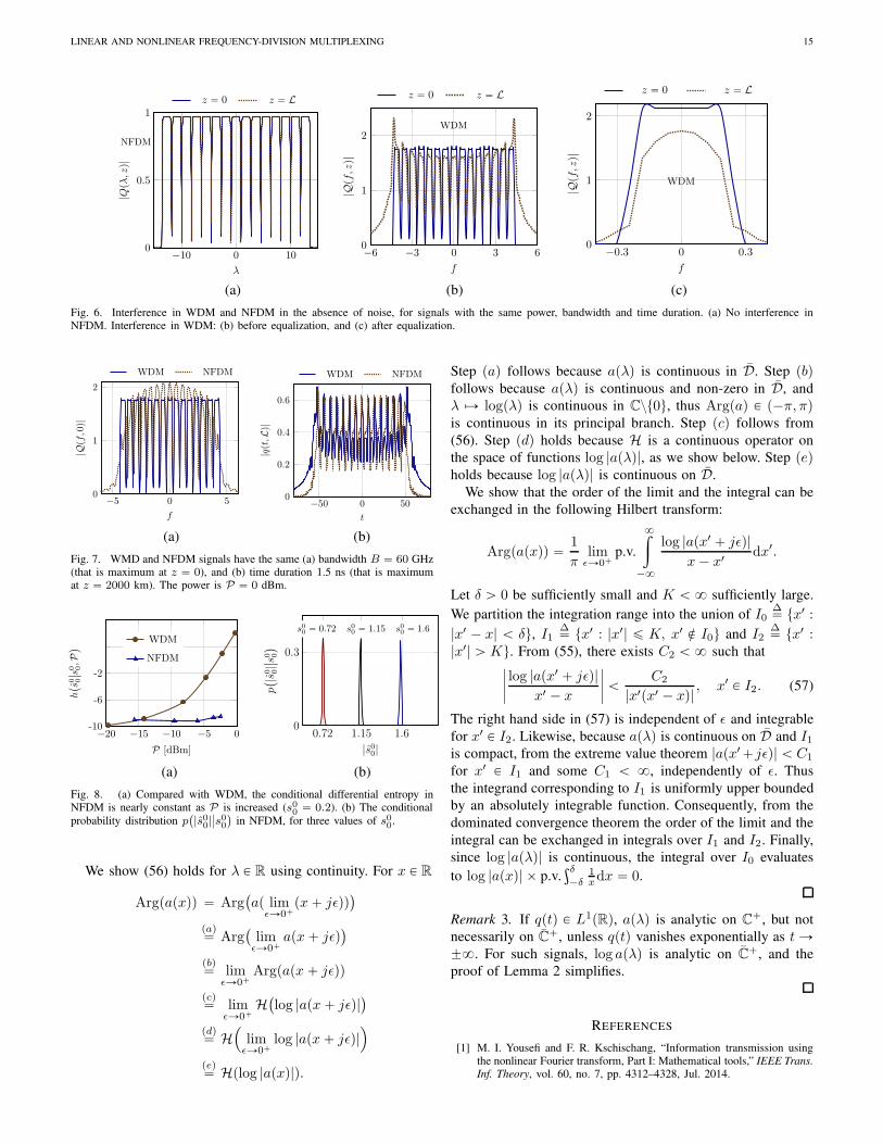
LINEAR AND NONLINEAR FREQUENCY-DIVISION MULTIPLEXING 15
´10 0 100
0.5
1
λ
|Qpλ,z
q|
z “ 0 z “ L
NFDM
´6 ´3 0 3 60
1
2
f
|Qpf,z
q|
z “ 0 z “ L
WDM
´0.3 0 0.30
1
2
f
|Qpf,z
q|
z “ 0 z “ L
WDM
(a) (b) (c)
Fig. 6. Interference in WDM and NFDM in the absence of noise, for signals with the same power, bandwidth and time duration. (a) No interference inNFDM. Interference in WDM: (b) before equalization, and (c) after equalization.
´5 0 50
1
2
f
|Qpf,0
q|
WDM NFDM
´50 0 500
0.2
0.4
0.6
t
|qpt,L
q|
WDM NFDM
(a) (b)
Fig. 7. WMD and NFDM signals have the same (a) bandwidth B “ 60 GHz(that is maximum at z “ 0), and (b) time duration 1.5 ns (that is maximumat z “ 2000 km). The power is P “ 0 dBm.
´20 ´15 ´10 ´5 0-10
-6
-2
P [dBm]
h`
s0 0
ˇ ˇ
s0 0,P
˘
WDM
NFDM
0.72 1.15 1.60
0.3
|s00|
p
`
|s0 0|ˇ ˇ
s0 0
˘
s0
0“ 0.72 s
0
0“ 1.15 s
0
0“ 1.6
(a) (b)
Fig. 8. (a) Compared with WDM, the conditional differential entropy inNFDM is nearly constant as P is increased (s00 “ 0.2). (b) The conditional
probability distribution p`
|s00|ˇ
ˇs00˘
in NFDM, for three values of s00.
We show (56) holds for λ P R using continuity. For x P R
Argpapxqq “ Arg`
ap limǫÑ0`
px ` jǫqq˘
paq“ Arg`
limǫÑ0`
apx ` jǫq˘
pbq“ limǫÑ0`
Argpapx ` jǫqqpcq“ lim
ǫÑ0`
H`
log |apx ` jǫq|˘
pdq“ H´
limǫÑ0`
log |apx ` jǫq|¯
peq“ Hplog |apxq|q.
Step paq follows because apλq is continuous in D. Step pbqfollows because apλq is continuous and non-zero in D, and
λ ÞÑ logpλq is continuous in Czt0u, thus Argpaq P p´π, πqis continuous in its principal branch. Step pcq follows from
(56). Step pdq holds because H is a continuous operator on
the space of functions log |apλq|, as we show below. Step peqholds because log |apλq| is continuous on D.
We show that the order of the limit and the integral can be
exchanged in the following Hilbert transform:
Argpapxqq “ 1
πlimǫÑ0`
p.v.
8ż
´8
log |apx1 ` jǫq|x ´ x1
dx1.
Let δ ą 0 be sufficiently small and K ă 8 sufficiently large.
We partition the integration range into the union of I0∆“ tx1 :
|x1 ´ x| ă δu, I1∆“ tx1 : |x1| ď K, x1 R I0u and I2
∆“ tx1 :
|x1| ą Ku. From (55), there exists C2 ă 8 such thatˇ
ˇ
ˇ
ˇ
log |apx1 ` jǫq|x1 ´ x
ˇ
ˇ
ˇ
ˇ
ă C2
|x1px1 ´ xq| , x1 P I2. (57)
The right hand side in (57) is independent of ǫ and integrable
for x1 P I2. Likewise, because apλq is continuous on D and I1is compact, from the extreme value theorem |apx1 `jǫq| ă C1
for x1 P I1 and some C1 ă 8, independently of ǫ. Thus
the integrand corresponding to I1 is uniformly upper bounded
by an absolutely integrable function. Consequently, from the
dominated convergence theorem the order of the limit and the
integral can be exchanged in integrals over I1 and I2. Finally,
since log |apλq| is continuous, the integral over I0 evaluates
to log |apxq| ˆ p.v.şδ
´δ1xdx “ 0.
Remark 3. If qptq P L1pRq, apλq is analytic on C`, but not
necessarily on C`, unless qptq vanishes exponentially as t Ñ˘8. For such signals, log apλq is analytic on C`, and the
proof of Lemma 2 simplifies.
REFERENCES
[1] M. I. Yousefi and F. R. Kschischang, “Information transmission usingthe nonlinear Fourier transform, Part I: Mathematical tools,” IEEE Trans.
Inf. Theory, vol. 60, no. 7, pp. 4312–4328, Jul. 2014.

16 YOUSEFI AND YANGZHANG
ℜs
ℑs 1.7
´1.42 ´0.71 0 0.71 1.42
¨1.41
´0.71
0
0.71
¨1.41P “ ´0.33 dBmNFDM
ℜs r?mWs
ℑs
r?mW
s
´1.42 ´0.71 0 0.71 1.42
¨1.41
´0.71
0
0.71
¨1.41P “ ´0.33 dBmWDM
ℜs r?mWs
ℑs
r?mW
s
(a) (b) (c)
Fig. 9. (a) Constellation for skℓ
in the U domain. Received symbols for four transmitted symbols in (b) NFDM, and (c) WDM.
[2] ——, “Information transmission using the nonlinear Fourier transform,Part II: Numerical methods,” IEEE Trans. Inf. Theory, vol. 60, no. 7,pp. 4329–4345, Jul. 2014.
[3] ——, “Information transmission using the nonlinear Fourier transform,Part III: Spectrum modulation,” IEEE Trans. Inf. Theory, vol. 60, no. 7,pp. 4346–4369, Jul. 2014.
[4] M. I. Yousefi, “Information transmission using the nonlinear Fouriertransform,” Ph.D. dissertation, University of Toronto, Mar. 2013.
[5] G. Boffetta and A. R. Osborne, “Computation of the direct scatteringtransform for the nonlinear Schrodinger equation,” J. Comp. Phys., vol.102, no. 2, pp. 252–264, Oct. 1992.
[6] M. J. Ablowitz, B. Prinari, and A. D. Trubatch, Discrete and Continuous
Nonlinear Schrodinger Systems, 1st ed., ser. Lond. Math. Soc. Lec. NoteSeries. Cambridge, UK: Cambridge University Press, 2003, vol. 302.
[7] M. I. Yousefi, “The Kolmogorov-Zakharov model for optical fibercommunication,” IEEE Trans. Inf. Theory, vol. 61, no. 1, pp. 377–391,Jan. 2017.
[8] A. Hasegawa and T. Nyu, “Eigenvalue communication,” IEEE J. Lightw.
Technol., vol. 11, no. 3, pp. 395–399, Mar. 1993.[9] E. Meron, M. Feder, and M. Shtaif, “On the achievable communica-
tion rates of generalized soliton transmission systems,” Arxiv peprint,
arXiv:1207.0297, pp. 1–13, Jul. 2012.
[10] J. E. Prilepsky, S. A. Derevyanko, K. J. Bluw, I. Gabitov, and S. K. Tu-ritsyn, “Nonlinear inverse synthesis and eigenvalue division multiplexingin optical fiber channels,” Phys. Rev. Lett., vol. 113, no. 1, pp. 013 901(1–5), Jul. 2014.
[11] S. Hari, M. I. Yousefi, and F. R. Kschischang, “Multieigenvalue com-munication,” IEEE J. Lightw. Technol., vol. 34, no. 13, pp. 3110–3117,Jul. 2016.
[12] Z. Dong, S. Hari, T. Gui, K. Zhong, M. I. Yousefi, C. Lu, P.-K. A. Wai,F. R. Kschischang, and A. P. T. Lau, “Nonlinear frequency divisionmultiplexed transmissions based on NFT,” IEEE Photon. Technol. Lett.,vol. 27, no. 15, pp. 1621–1623, Aug. 2015.
[13] R. G. Gallager, Principles of Digital Communication. Cambridge, UK:Cambridge University Press, 2008.
[14] S. T. Le, J. E. Prilepsky, and S. K. Turitsyn, “Nonlinear inverse synthesisfor high spectral efficiency transmission in optical fibers,” Opt. Exp.,vol. 22, no. 22, pp. 26 720–26 741, Nov. 2014.
[15] S. T. Le, S. Wahls, D. Lavery, J. E. Prilepsky, and S. K. Turitsyn,“Reduced complexity nonlinear inverse synthesis for nonlinearity com-pensation in optical fiber links,” in The European Conf. Lasers Electro-
Optics, Munich, Germany, Jun. 2015.
[16] H. Bulow, V. Aref, and L. Schmalen, “Modulation on discrete nonlinearspectrum: Perturbation sensitivity and achievable rates,” IEEE Photon.Technol. Lett., vol. 30, no. 5, pp. 423 –426, Mar. 2018.
[17] H. Buelow, V. Aref, and W. Idler, “Transmission of waveforms deter-mined by 7 eigenvalues with PSK-modulated spectral amplitudes,” inEuropean Conf. on Opt. Commun., Dusseldorf, Germany, Sep. 2016,pp. 1–3.
[18] V. Aref, H. Buelow, K. Schuh, and W. Idler, “Experimental demon-stration of nonlinear frequency division multiplexed transmission,” inEuropean Conf. Opt. Commun., Valencia, Spain, Sep. 2015, pp. 1–3.
[19] V. Aref, “Control and detection of discrete spectral amplitudes innonlinear Fourier spectrum,” arXiv: 1605.06328, May 2016.
[20] H. Terauchi and A. Maruta, “Eigenvalue modulated optical transmis-sion system based on digital coherent technology,” in Joint OptoElec.
Commun. Conf. & 2013 Int. Conf. Photonics in Switching (OECC/PS),Kyoto, Japan, Jul. 2013, pp. 1–2.
[21] A. Span, V. Aref, H. Bulow, and S. T. Brink, “On time-bandwidthproduct of multi-soliton pulses,” in IEEE Int. Symp. Info. Theory,Aachen, Germany, Jun. 2017, pp. 61–65.
[22] W. Q. Zhang et al., “Correlated eigenvalues optical communications,”Arxiv preprints, arXiv:1711.09227, pp. 1–14, Nov. 2017.
[23] J. Garcia, “Communication using eigenvalues of higher multiplicity ofthe nonlinear Fourier transform,” ArXiv preprint, arXiv:1802.07456, pp.1–8, Feb. 2018.
[24] V. Aref, S. T. Le, and H. Buelow, “Demonstration of fully nonlinearspectrum modulated system in the highly nonlinear optical transmissionregime,” in European Conf. on Opt. Commun., Dusseldorf, Germany,Sep. 2016, pp. 1–3.
[25] I. Tavakkolnia and M. Safari, “Signalling over nonlinear fibre-opticchannels by utilizing both solitonic and radiative spectra,” in European
Conf. Networks and Commun., Paris, France, Jul. 2015, pp. 103–107.
[26] V. Aref, S. T. Le, and H. Buelow, “Modulation over nonlinear fourierspectrum: Continuous and discrete spectrum,” IEEE J. Lightw. Technol.,vol. 36, no. 6, pp. 1289–1295, Mar. 2018.
[27] Q. Zhang and T. H. Chan, “A spectral domain noise model for opticalfibre channels,” in IEEE Int. Symp. Info. Theory, Hong Kong, Jun. 2015,pp. 1660–1664.
[28] Q. Zhang, T. H. Chan, and A. Grant, “Spatially periodic signals for fiberchannels,” in IEEE Int. Symp. Info. Theory, Honolulu, HI, USA, Jun.2014, pp. 2804–2808.
[29] S. Civelli, E. Forestieri, and M. Secondini, “Decision-feedback detectionstrategy for nonlinear frequency-division multiplexing,” arXiv preprint,arXiv:1801.05338, 2018.
[30] ——, “A novel detection strategy for nonlinear frequency-divisionmultiplexing,” in Opt. Fiber Commun. Conf., San Diego, CA, USA,Mar. 2018, pp. 1–3.
[31] P. Kazakopoulos and A. L. Moustakas, “Nonlinear Schrodinger equationwith random Gaussian input: Distribution of inverse scattering data andeigenvalues,” Phys. Rev. E, vol. 78, no. 1, pp. 016 603 (1–7), Jul. 2008.
[32] S. Civelli, E. Forestieri, and M. Secondini, “Why noise and dispersionmay seriously hamper nonlinear frequency-division multiplexing,” IEEE
Photon. Technol. Lett., vol. 29, no. 16, pp. 1332–1335, Aug. 2017.
[33] X. Yangzhang, D. Lavery, P. Bayvel, and M. I. Yousefi, “Impact ofperturbations on nonlinear frequency-division multiplexing,” IEEE J.Lightw. Technol., vol. 36, no. 2, pp. 485–494, Jan. 2018.
[34] V. Aref, S. T. Le, and H. Bulow, “Does the cross-talk between nonlinearmodes limit the performance of NFDM systems?” in European Conf.
on Opt. Commun., Sep. 2017, pp. 1–3.[35] R. T. Jones, S. Gaiarin, M. P. Yankov, and D. Zibar, “Noise robust
receiver for eigenvalue communication systems,” in Opt. Fiber Commun.
Conf., San Diego, CA, USA, Mar. 2018, pp. W2A–59.
[36] A. M. Bruckstein, B. C. Levy, and T. Kailath, “Differential methods ininverse scattering,” SIAM J. Appl. Math., vol. 45, no. 2, pp. 312–335,Apr. 1985.
[37] J. Skaar and O. H. Waagaard, “Design and characterization of finite-length fiber gratings,” IEEE J. Quantum Electron., vol. 39, no. 10, pp.1238–1245, Oct. 2003.
[38] A. Rosenthal and M. Horowitz, “Inverse scattering algorithm for re-constructing strongly reflecting fiber Bragg gratings,” IEEE J. Quantum
Electron., vol. 39, no. 8, pp. 1018–1026, Aug. 2003.

LINEAR AND NONLINEAR FREQUENCY-DIVISION MULTIPLEXING 17
[39] A. Buryak, J. Bland-Hawthorn, and V. Steblina, “Comparison of inversescattering algorithms for designing ultrabroadband fibre bragg gratings,”Opt. Exp., vol. 17, no. 3, pp. 1995–2004, Feb. 2009.
[40] S. Civelli, L. Barletti, and M. Secondini, “Numerical methods for theinverse nonlinear Fourier transform,” in Tyrrhenian Int. Workshop on
Digital Commun., Florence, Italy, Sep. 2015, pp. 13–16.[41] S. Wahls and H. V. Poor, “Fast numerical nonlinear Fourier transforms,”
IEEE Trans. Inf. Theory, vol. 61, no. 12, pp. 6957–6974, Dec. 2015.[42] ——, “Fast inverse nonlinear Fourier transform for generating multi-
solitons in optical fiber,” in IEEE Int. Symp. Info. Theory, Hong Kong,China, Jun. 2015, pp. 1676–1680.
[43] S. Wahls, S. T. Le, J. E. Prilepsky, H. V. Poor, and S. K. Turitsyn,“Digital backpropagation in the nonlinear Fourier domain,” in IEEEInt. Workshop Signal Process. Advances Wireless Commun., Stockholm,Sweden, Jun. 2015, pp. 445–449.
[44] V. Vaibhav, “Fast inverse nonlinear Fourier transform,” ArXiv preprint,
arXiv:1706.04069, Jun. 2017.[45] S. Gaiarin, A. M. Perego, E. P. da Silva, F. D. Ros, and D. Zibar,
“Experimental demonstration of dual polarization nonlinear frequencydivision multiplexed optical transmission system,” in European Conf.on Opt. Commun., Gothenburg, Sweden, Sep. 2017, pp. 1–3.
[46] S. Gaiarin, A. M. Perego, E. P. da Silva, F. Da Ros, and D. Zibar, “Dual-polarization nonlinear Fourier transform-based optical communicationsystem,” Optica, vol. 5, no. 3, pp. 263–270, Mar. 2018.
[47] J.-W. Goossens, M. I. Yousefi, Y. Jaouen, and H. Hafermann,“Polarization-division multiplexing based on the nonlinear Fourier trans-form,” Opt. Exp., vol. 25, no. 22, pp. 26 437–26 452, Oct. 2017.
[48] M. Kamalian, J. E. Prilepski, S. T. Le, and S. Turitsyn, “Periodicnonlinear Fourier transform for fiber-optic communications, Part I–II,”Opt. Exp., vol. 24, no. 16, pp. 18 353–18 381, Aug. 2016.
[49] N. A. Shevchenko et al., “A lower bound on the per soliton capacityof the nonlinear optical fibre channel,” in IEEE Info. Theory Workshop,Jeju Island, South Korea, Oct. 2015, pp. 1–5.
[50] P. Kazakopoulos and A. L. Moustakas, “On the soliton spectral efficiencyin non-linear optical fibers,” in IEEE Int. Symp. Info. Theory, Barcelona,Spain, Jul. 2016, pp. 610–614.
[51] I. Tavakkolnia and M. Safari, “Capacity analysis of signaling on the con-tinuous spectrum of nonlinear optical fibers,” IEEE J. Lightw. Technol.,vol. 35, no. 11, pp. 2086–2097, Jun. 2017.
[52] S. A. Derevyanko, J. E. Prilepsky, and S. K. Turitsyn, “Capacity esti-mates for optical transmission based on the nonlinear Fourier transform,”Nature Commun., vol. 7, no. 12710, pp. 1–9, Sep. 2016.
[53] ——, “Capacity estimates for optical transmission based on the nonlin-ear fourier transform,” Nature Commun., vol. 7, Sep. 2016, Paper no.12710.
[54] P. Kazakopoulos and A. L. Moustakas, “On the soliton spectral efficiency
in non-linear optical fibers,” in IEEE Int. Symp. Info. Theory, Barcelona,Spain, Jul. 2016, pp. 610–614.
[55] H. Bulow, “Nonlinear Fourier transformation based coherent detectionscheme for discrete spectrum,” in Opt. Fiber Commun. Conf. andExposition, Los Angeles, CA, USA, Mar. 2015, pp. 1–3.
[56] ——, “Experimental assessment of nonlinear Fourier transformationbased detection under fiber nonlinearity,” in European Conf. Opt. Com-
mun., Cannes, France, Sep. 2014, pp. 1–3.[57] H. Bulow, “Experimental demonstration of optical signal detection using
nonlinear Fourier transform,” IEEE J. Lightw. Technol., vol. 33, no. 7,pp. 1433–1439, Apr. 2015.
[58] A. Maruta, A. Toyota, Y. Matsuda, and Y. Ikeda, “Experimental demon-stration of long haul transmission of eigenvalue modulated signals,” inTyrrhenian Int. Workshop on Digital Commun., Sep. 2015, pp. 28–30.
[59] T. Gui et al., “Polarization-division-multiplexed nonlinear frequencydivision multiplexing,” in The Conf. Lasers Electro-Optics, San Jose,CA, USA, May 2018, pp. 1–2.
[60] S. T. Le, H. Buelow, and V. Aref, “Demonstration of 64ˆ 0.5 Gbaudnonlinear frequency division multiplexed transmission with 32QAM,”in Opt. Fiber Commun. Conf., Los Angeles, CA, USA, Mar. 2017, pp.1–3.
[61] S. T. Le, V. Aref, and H. Buelow, “High speed precompensated nonlinearfrequency-division multiplexed transmissions,” IEEE J. Lightw. Technol.,vol. 36, no. 6, pp. 1296–1303, Mar. 2018.
[62] X. Yangzhang, M. I. Yousefi, A. Alvarado, D. Lavery, and P. Bayvel,“Nonlinear frequency-division multiplexing in the focusing regime,” inOpt. Fiber Commun. Conf., Los Angeles, USA, Mar. 2017, pp. 1–3.
[63] G. P. Agrawal, Nonlinear Fiber Optics, 4th ed. San Francisco, CA,USA: Academic, 2007.
[64] A. Splett, C. Kurtzke, and K. Petermann, “Ultimate transmission capac-ity of amplified optical fiber communication systems taking into accountfiber nonlinearities,” in European Conf. Opt. Commun., Montreux,Switzerland, Sep 1993, pp. 41–44.
[65] R. J. Essiambre, G. Kramer, P. J. Winzer, G. J. Foschini, and B. Goebel,“Capacity limits of optical fiber networks,” IEEE J. Lightw. Technol.,vol. 28, no. 4, pp. 662–701, Feb. 2010.
[66] E. Agrell, “Conditions for a monotonic channel capacity,” IEEE Trans.
Commun., vol. 63, no. 3, pp. 1–11, Sep. 2015.[67] J. Tang, “The Shannon channel capacity of dispersion-free nonlinear
optical fiber transmission,” IEEE J. Lightw. Technol., vol. 19, no. 8, pp.1104–1109, Aug. 2001.
[68] G. D. Forney, Jr., “Principles of digital communication II.” Mas-sachusetts Institute of Technology, Mar. 2005, MIT OpenCourseWare,Course no. 6.451, Lecture Notes.
[69] M. I. Yousefi, “The asymptotic capacity of the optical fiber,” Arxivpreprint, arXiv:1610.06458, pp. 1–12, Nov. 2016.