
Linear and Nonlinear Electromagnetic Responses in ... · Linear and Nonlinear Electromagnetic...
83
Linear and Nonlinear Electromagnetic Responses in Topological Semimetals by Shudan Zhong A dissertation submitted in partial satisfaction of the requirements for the degree of Doctor of Philosophy in Physics in the Graduate Division of the University of California, Berkeley Committee in charge: Professor Joel E. Moore, Chair Professor Dung-Hai Lee Professor Maciej Zworski Fall 2018
Transcript of Linear and Nonlinear Electromagnetic Responses in ... · Linear and Nonlinear Electromagnetic...

Linear and Nonlinear Electromagnetic Responses in Topological Semimetals
by
Shudan Zhong
A dissertation submitted in partial satisfaction of the
requirements for the degree of
Doctor of Philosophy
in
Physics
in the
Graduate Division
of the
University of California, Berkeley
Committee in charge:
Professor Joel E. Moore, ChairProfessor Dung-Hai LeeProfessor Maciej Zworski
Fall 2018
Linear and Nonlinear Electromagnetic Responses in Topological Semimetals
Copyright 2018by
Shudan Zhong

1
Abstract
Linear and Nonlinear Electromagnetic Responses in Topological Semimetals
by
Shudan Zhong
Doctor of Philosophy in Physics
University of California, Berkeley
Professor Joel E. Moore, Chair
The topological consequences of time reversal symmetry breaking in two dimensionalelectronic systems have been a focus of interest since the discovery of the quantum Halleffects. Similarly interesting phenomena arise from breaking inversion symmetry in threedimensional systems. For example, in Dirac and Weyl semimetals the inversion symmetrybreaking allows for non-trivial topological states that contain symmetry-protected pairs ofchiral gapless fermions. This thesis presents our work on the linear and nonlinear electro-magnetic responses in topological semimetals using both a semiclassical Boltzmann equationapproach and a full quantum mechanical approach. In the linear response, we find a “gy-rotropic magnetic effect” (GME) where the current density jB in a clean metal is inducedby a slowly-varying magnetic field. It is shown that the experimental implications and mi-croscopic origin of GME are both very different from the chiral magnetic effect (CME). Wedevelop a systematic way to study general nonlinear electromagnetic responses in the low-frequency limit using a Floquet approach and we use it to study the circular photogalvaniceffect (CPGE) and second-harmonic generation (SHG). Moreover, we derive a semiclassicalformula for magnetoresistance in the weak field regime, which includes both the Berry cur-vature and the orbital magnetic moment. Our semiclassical result may explain the recentexperimental observations on topological semimetals. In the end, we present our work onthe Hall conductivity of insulators in a static inhomogeneous electric field and we discuss itsrelation to Hall viscosity.

i
To my grandfather,

ii
Contents
Acknowledgement iv
1 Introduction 11.1 Background and motivation . . . . . . . . . . . . . . . . . . . . . . . . . . . 11.2 Overview . . . . . . . . . . . . . . . . . . . . . . . . . . . . . . . . . . . . . . 21.3 List of publications . . . . . . . . . . . . . . . . . . . . . . . . . . . . . . . . 3
2 Preliminaries 42.1 Berry phase . . . . . . . . . . . . . . . . . . . . . . . . . . . . . . . . . . . . 42.2 Semiclassical theory . . . . . . . . . . . . . . . . . . . . . . . . . . . . . . . . 5
2.2.1 Bloch waves . . . . . . . . . . . . . . . . . . . . . . . . . . . . . . . . 52.2.2 Semiclassical equations . . . . . . . . . . . . . . . . . . . . . . . . . . 52.2.3 Example: the response to a static magnetic field . . . . . . . . . . . . 8
3 Gyrotropic magnetic effect and the magnetic moment on the Fermi sur-face 93.1 Introduction . . . . . . . . . . . . . . . . . . . . . . . . . . . . . . . . . . . . 93.2 Chiral magnetic effect versus gyrotropic magnetic effect . . . . . . . . . . . . 11
3.2.1 Chiral magnetic effect . . . . . . . . . . . . . . . . . . . . . . . . . . 113.2.2 Gyrotropic magnetic effect . . . . . . . . . . . . . . . . . . . . . . . . 13
3.3 Semiclassical picture of the gyrotropic magnetic effect . . . . . . . . . . . . . 153.4 Applications in topological semimetals . . . . . . . . . . . . . . . . . . . . . 163.5 Supplemental material for gyrotropic magnetic effect . . . . . . . . . . . . . 18
3.5.1 Kubo formula for natural gyrotropy in crystals . . . . . . . . . . . . . 183.5.2 Low-frequency natural gyrotropic response without dissipation . . . . 203.5.3 Low-frequency natural gyrotropic response with dissipation . . . . . . 243.5.4 Orbital GME in two-band models: comparison with the previous lit-
erature . . . . . . . . . . . . . . . . . . . . . . . . . . . . . . . . . . . 263.5.5 Natural optical activity of metals in the semiclassical limit . . . . . . 27
3.5.5.1 Gyrotropic response in equilibrium . . . . . . . . . . . . . . 273.5.5.2 Nonequilibrium optical gyrotropy in Weyl semimetals driven
by the chiral anomaly . . . . . . . . . . . . . . . . . . . . . 28

iii
3.5.5.3 Reciprocity relation for a metal with a smooth interface . . 293.5.5.4 Berry-curvature contributions . . . . . . . . . . . . . . . . . 31
4 Magnetoresistance and nonlinear optical responses in metals 344.1 Introduction . . . . . . . . . . . . . . . . . . . . . . . . . . . . . . . . . . . . 344.2 Nonlinear optical effects and Floquet approach . . . . . . . . . . . . . . . . 36
4.2.1 Geometrical meaning of nonlinear optics in the semiclassical approach 364.2.2 Fully quantum mechanical derivation by Floquet formalism . . . . . . 37
4.3 Semiclassical formulas for magnetoconductance . . . . . . . . . . . . . . . . 444.4 Angle-dependent magnetoresistance . . . . . . . . . . . . . . . . . . . . . . 484.5 Supplemental material for derivation of the Berry curvature dipole formula
for general bands . . . . . . . . . . . . . . . . . . . . . . . . . . . . . . . . . 49
5 Hall conductivity in an inhomogeneous electric field 565.1 Preliminaries and background . . . . . . . . . . . . . . . . . . . . . . . . . . 565.2 Derivation of the q2 term in Hall conductivity . . . . . . . . . . . . . . . . . 58
5.2.1 Symmetry analysis . . . . . . . . . . . . . . . . . . . . . . . . . . . . 585.2.2 Derivation using Kubo formula . . . . . . . . . . . . . . . . . . . . . 59
5.3 Semiclassical derivation . . . . . . . . . . . . . . . . . . . . . . . . . . . . . . 645.4 Numerical results for Chern insulators . . . . . . . . . . . . . . . . . . . . . 67
5.4.1 Topological flat band model . . . . . . . . . . . . . . . . . . . . . . . 675.4.2 Hofstadter model . . . . . . . . . . . . . . . . . . . . . . . . . . . . . 67
Bibliography 72

iv
Acknowledgments
First, I would like to express my sincerest gratitude to my thesis advisor Prof. Joel E. Moorefor his guidance and support during my Ph.D study. I have been inspired by his deep insightin physics and deeply touched by his kindness in every aspect. I am thankful for his patienceand the amount of freedom he has given me in research. Besides, I would like to especiallythank his financial support for spending his valuable time on funding. I am grateful for beingone of his students.
I am indebted to my other collaborators, Ivo Souza, Takahiro Morimoto, and JosephOrenstein. Much of the credit for the results presented in this thesis should be attributed tothem. I also thank my other thesis and qualification committee members, Prof. Dung-HaiLee, Prof. Maciej Zworski and Prof. Joseph Orenstein for intriguing discussions. I owe muchto Prof. Yuanming Lu and Prof. Ashvin Vishvanath for the guidance when I was a freshgraduate student. I thank Prof. Hitoshi Murayama, Prof. Dung-Hai Lee and many otherprofessors in Berkeley physics department for the enlightening courses. I appreciate the hardwork of the Berkeley physics department staff. In particular, I would like to thank AnneTakizawa, Donna K. Sakima, and Joelle Miles for their kind help.
I would also like to thank my officemates, friends in Berkeley, and people at the fifthfloor of Birge Hall: Benjamin Ponedel, Ziqi Yan, Fang Fang, Felix Flicker, Benjamin M.Fregoso, Byungmin Kang, Aaron Szasz, Michael P Zaletel, Yichen Huang, Daniel Varjas,Sylvia Lewin, Ting Cao, and many others. My wonderful memories with them will lastforever.
Finally, I can never thank enough to my family for their love and support.

1
Chapter 1
Introduction
1.1 Background and motivation
According to the electronic properties, solid materials are divided into insulators, semicon-ductors, semimetals and metals (conductors). During the past decade, topology has becomean important role in defining new phases of the matter and a new phase of matter called topo-logical insulators has started to spurring researchers’ interest. Different from conventionalinsulators, topological insulators have gapless surface states and quantized electronic re-sponse functions. These properties are protected by topology, meaning that under a smoothdeformation (with the insulating gap open) of the Hamiltonian without breaking certainsymmetries one can not turn a topological class of insulators into another class, for example,turning the topological insulators into conventional trivial insulators.
Similarly interesting phenomena have been found beyond insulating phases recently. Anexample is the Weyl semimetal in three dimensional space. In the band structure of a Weylsemimetal the conduction bands and valence bands intersect at isolated points. Those gap-less points named as Weyl nodes are topologically protected in the sense that one can nottransform a Weyl semimetal into an insulator by small perturbations when charge conserva-tion and transnational invariance is preserved. Weyl semimetals also have protected surfacestates as in topological insulators.
The protection can be seen more clearly if one looks close to the Hamiltonian near aWeyl node at momentum k∗:
H =∑ij
~σibij(kj − k∗j ) (1.1)
where σi are Pauli matrices in the basis of the two bands involved and bij are some realparameters. As we can see, all Pauli matrices have been used up in this Hamiltonian, so onecan not gap out the spectrum by adding anticommuting matrices. Using this Hamiltonianone can also define the chirality of the Weyl node by χ = sign det bij. The chirality is themagnetic charge of a Weyl node: if one integrate the Berry curvature (It is like the magneticfield and we will talk more about it in the next chapter. ) over a closed surface enclosing

CHAPTER 1. INTRODUCTION 2
the Weyl node the value will be 2πχ.Recently, the condensed matter community has been actively studying the unusual trans-
port and optical phenomena in Weyl semimetals. One important example is the chiral mag-netic effect (CME) where Weyl nodes with different chemical potentials and a static magneticfield give rise to an electric current parallel to the magnetic field. Another example is thenegative magnetoresistance where an applied static magnetic field leads to a large magne-toresistance with unusual anisotropy. However, these phenomena in Weyl semimetals hasnot been fully understood. In this thesis, we will try addressing the following concerns: (i)Recently, there is a claim stating that, in Weyl semimetals, a static magnetic field by itself issufficient to drive a dissipationless current. Such an effect has been characterized as a typeof CME. However, even the existence of this type of CME is questionable since it violatesthe Bloch theorem, which forbids the macroscopic currents in a bulk system in equilibrium.While this has been actively debated, no thorough study has been carried out. (ii) Recent re-search on the negative magnetoresistance in weak magnetic field using semiclassical approachhas considered only chiral anomaly (or Berry curvature). However, in a complete analysis,another important component—orbital magnetic moment [67]—is indispensable. (iii) Thesemiclassical approach (SCA) has been used to study the nonlinear optical responses in met-als. The SCA conserves the properly defined volume in phase space and gives an intuitiveapproach to many observable properties of metals. However, the SCA can make erroneouspredictions if used on nonlinear optical responses in metals. A full quantum theory approachis necessary to confirm the validity of the results derived by the SCA.
In addition to studying the topological properties of the topological phases, an active areaof the recent research has been studying the geometrical properties of the topological phase,such as the Hall viscosity. One question remained for the Hall viscosity is how to measureit in experiment. Recent work[66, 15] shows that the Hall conductivity in an inhomogenouselectric field receives a contribution from the Hall viscosity. Therefore, the Hall viscositycan be determined by measuring the the Hall conductivity. At the end of this thesis we willpresent our work on the study of Hall conductivity in a inhomogenous electric field.
1.2 Overview
In this section we give an overview of the following chapters in this thesis.Chapter 2 gives a brief review of the Berry phase, Berry curvature, quantum geometric
tensor, and quantum metric tensor. We give a short introduction of the semiclassical theory,a tool we will use in the following chapters. At the end of this chapter we give an exampleof using semiclassical equations to solve a transport problem in metals.
In Chapter 3, we study the linear electromagnetic response in metals using semiclassicalapproach and a full quantum derivation. We find a “gyrotropic magnetic effect” (GME)where the current density jB in a clean metal is induced by a slowly-varying magnetic field.We make a distinction between the chiral magnetic effect (CME) and GME. and by doingthis we confirm that there can not be a dissipationless current in equilibrium. In the end

CHAPTER 1. INTRODUCTION 3
we work on a simple two band model of the Weyl semimetals and discuss the realizationof GME as the low frequency limit of natural optical activity (NOA) on mirror-free Weylsemimetals.
In the supplemental material, we give the technical details of using Kubo formula tocalculate the linear-response of natural gyrotropy in metals at low frequencies. We also givethe derivation of a formula for the equilibrium optical activity coefficient of an isotropicWeyl semimetal and the derivation of a formula for the nonequilibrium optical gyrotropyof a Weyl semimetal due to the chiral anomaly. In addition to the technical details, wediscuss the reciprocity relation for a metal. The Onsager reciprocity principle requires thatin T -invariant materials there is no optical rotation in reflection (Kerr effect). We show howthis principle is reflected in our semiclassical results.
In Chapter 4, we study the angle-dependent magnetoresistance in topological semimet-als using a semiclassical approach. We apply our semiclassical result on the Hamiltonianfor a Weyl semimetal and show that our result captures the directional anisotropy of lin-ear conductivity under a magnetic field, which may explain the low-field regime of recentexperiments. In this chapter we also study the nonlinear optical responses using a Floquetapproach. Our approach reproduces the semiclassical formula for the circular photogalvaniceffect (CPGE) and provides a systematic way to study general nonlinear electromagneticresponses in the low-frequency limit.
Chapter 5 studies the Hall conductivity of insulators in an inhomogeneous electric fieldto the second order of the wave number q using both the Kubo formula and the semiclassicalapproach. We show that in a special case when the system have only two bands and when thebands are all flat the q2 term of the Hall conductivity is fully determined by an interplay ofthe Berry curvature and the quantum metric tensor. In the end we do numerical studies onthe Chern insulators and discuss the relation between Hall conductivity and Hall viscosity.
1.3 List of publications
We list the publications for this thesis:
1. Semiclassical theory of nonlinear magneto-optical responses with applications to topo-logical Dirac/Weyl semimetals, Takahiro Morimoto, Shudan Zhong, Joseph Orensteinand Joel E. Moore, Phys. Rev. B, 94, 245121 (2016).
2. Gyrotropic magnetic effect and the orbital moment on the Fermi surface,Shudan Zhong,Joel E. Moore, and Ivo Souza, Physical Review Letter, 116, 077201 (2016).
3. Optical Gyrotropy from Axion Electrodynamics in Momentum Space, Shudan Zhong,Joseph Orenstein and Joel E. Moore, Physical Review Letter, 115, 117403 (2015).

4
Chapter 2
Preliminaries
In this chapter, We will briefly review some basic techniques and concepts used in this thesis.
2.1 Berry phase
In 1984, Berry brings a geometrical phase factor to physicists’ attention in his famous pa-per [11]. In the paper, the geometrical phase factor is shown exists in the adiabatic evolutionof a quantum system in an eigenstate when the path of the evolution makes up a circuit inthe Hamiltonian’s parameter space. The phase is also called Berry phase and it origins fromthe nontrivial topological property of the parameter space. One example is the Aharonov-Bohm(AB) effect where the Berry phase is given by a line integral of the vector potential Aalong a closed loop,
φ =q
~
∮C
A(R) · dR . (2.1)
This phase is gauge invariant and hence physical. One can check it by turning the lineintegral into a surface integral of the magnetic field B. Indeed, Berry phase can generallybe written as an integral of a field on the parameter space. The field is the Berry curvature.Berry curvature is also gauge invariant and it is the antisymmetric part of a gauge invariantquantum geometric tensor [12]
Tij = 〈∂in|(1− |n〉〈n|)|∂jn〉 (2.2)
where |n〉 denotes an eigenstate. The symmetric part of this tensor is called the quantummetric tensor. It provides a natural means to measure the distances between states.
CHAPTER 2. PRELIMINARIES 5
2.2 Semiclassical theory
2.2.1 Bloch waves
In a crystal, atoms form a lattice which has discrete translational symmetry. The electronsin a lattice will feel a periodic potential
V (r + R) = V (r) (2.3)
where R is a lattice vector. With the assumption that the electrons we consider are free,meaning that they do not interact with each other (the interactions between electrons isassumed to be represented by an effective one electron potential that is included in V ),the eigenstates of the Hamiltonian for this system will be Bloch waves according to Bloch’stheorem
HΨnk(r) = εnkΨnk(r), Ψnk(r) = eik·runk(r) . (2.4)
The unk(r) is periodicunk(r + R) = unk(r) . (2.5)
One can check that Ψnk is also the eigenstate of the translational operator T , which can beinferred from group theory
TΨnk(r + R) = Ψnk(r + R) = eik·(r+R)unk(r + R) = eik·RΨnk(r) . (2.6)
As a consequence, the k is called the crystal momentum.The set of all vectors G that satisfied
G ·R = 2πN, N ∈ Z (2.7)
gives the reciprocal lattice. It can be shown that k is periodic: k + G is the same as k.Therefore, we usually limit the values of k to be in any primitive unit cell of the reciprocallattice. There is one specific choice of the primitive unit cell called the Brillouin zone.
2.2.2 Semiclassical equations
In semiclassical theory, an electron is modeled as a wave packet. The wave packet is con-structed from Bloch waves
|Ψ(rc,kc)〉 =
∫[dk] a(k)Ψnk(r, t) . (2.8)
It is centered at rc in real space and kc in momentum space. a(k) is arbitrary function of kas long as the spread of the wave packet in k space is narrow compared with the Brillouinzone.
CHAPTER 2. PRELIMINARIES 6
The semiclassical equations of motion for the centers rc and kc of an electron wave packetare [67]
r =1
~∇kεk − k ×Ω, (2.9)
k = −eE − er ×B. (2.10)
where
Ω = −Im[〈∇kuk| × |∇kuk〉] (2.11)
is the Berry curvature and the electron charge is (−e). We omit the subscript c for the wavepacket centers and n for the Bloch waves.
From the symmetry of these equations between position and momentum, it is clear thatΩ(k) can be viewed as an effective magnetic field in momentum space and the magnetic fieldis the Berry curvature in real space.
One can see this symmetry more clearly with the Berry connection defined as
A(k) = i〈uk|∇k|uk〉 . (2.12)
The Berry connection can be viewed as the vector potential A in momentum space. TheBerry curvature will be given by
Ω(k) = ∇k ×A(k) . (2.13)
We know that in real space the Schrodinger equation
i∂tΨ(r, t) = H(r)Ψ(r, t) = −∇2
2mΨ(r, t) + V (r)Ψ(r, t) (2.14)
is invariant under a global phase shift
Ψ(r, t)→ eiφΨ(r, t) (2.15)
since φ is a constant. In addition, the Schrodinger equation is also invariant under localphase shift if it is for a charge particle. If we do a local phase shift to the wave function ofa charge particle
Ψ(r, t)→ eiφ(r,t)Ψ(r, t) (2.16)
the Schrodinger equation will be invariant if we also do a gauge transformation of the po-tential ϕ and A
ϕ′ = ϕ− 1
q∂tφ(r, t)
A′ = A +1
q∇φ(r, t) . (2.17)
CHAPTER 2. PRELIMINARIES 7
One can check that
(i∂t − qϕ′)eiφ(r,t)Ψ(r, t) = eiφ(r,t)(i∂t − qϕ′ − ∂tφ(r, t))Ψ(r, t) (2.18)
[1
2m(−i∇− qA′)2 + V ]eiφ(r,t)Ψ(r, t) = eiφ(r,t)[
1
2m(−i∇− qA′ +∇φ(r, t))2 + V ]Ψ(r, t) .
(2.19)
With Eq. (2.17) we have
(i∂t − qϕ′)eiφ(r,t)Ψ(r, t) = [1
2m(−i∇− qA′)2 + V ]eiφ(r,t)Ψ(r, t) (2.20)
indicating that the Schrodinger equation is invariant. Using Eq. (2.12) a similar transforma-tion can be done for a Bloch wave
|uk〉 → eiφ(k)|uk〉A → A−∇kφ(k) . (2.21)
The minus sign can be removed by redefining A but we would like to keep the currentdefinition for it is used in the following chapters. It can be shown that the Bloch wave witha local phase shift is still the solution of the Hamiltonian. The symmetry between positionand momentum in semiclassical equations can then be seen more clearly from
r = ∇kεk − k× (∇k ×A)
k = e∇rφ− er× (∇r ×A) . (2.22)
There are two more important things one should pay attention to when using the semi-classical equations. One is that the energy εk in Eq. (2.10) has a contribution from theorbital magnetic moment [67],
εk = ε0k −mk ·B (2.23)
where Hk|uk〉 = ε0k|uk〉 with B = 0 and the orbital magnetic moment is given by
mk = −e2
Im[〈∇kuk| × (Hk − ε0k)|∇kuk〉]. (2.24)
The orbital magnetic moment represents the self-rotation of a wave packet.The other thing is that one should use a modified phase-space density which is induced
by an external magnetic field [77]
D = 1 + eB ·Ω (2.25)
in order to have the phase space volume conserved.

CHAPTER 2. PRELIMINARIES 8
2.2.3 Example: the response to a static magnetic field
The semiclassical equations with the Boltzmann equation have been successfully used tounderstand various transport phenomena of solids, such as Haas-van Alphen oscillation,anomalous Hall effect, etc. In this section, we will give an example of using semiclassicalequations to study the response to a static magnetic field.
In the presence of a static magnetic field, the electrons are in an equilibrium state withthe distribution function f(εk). We solve r using Eq. (2.10):
r =1
D[∇kεk + e(∇kεk ·Ω)B] . (2.26)
Note that εk = ε0k −mk ·B. The current density j is given by
j = −e∫
[dk]Df(εk)r . (2.27)
Focusing on the terms linear in B we will have
j = −e∫
[dk]f(εk)[∇kεk + e(∇kεk ·Ω)B] (2.28)
= −e∫
[dk]f(ε0)v0k + f(ε0)∇k(−mk ·B) +
∂f(ε0)
∂ε0(−m ·B)vk + f(ε0)e(vk ·Ω)B (2.29)
where vk = ∂kε0. The first term gives zero. The second and third term cancel each other
after we do integral by parts. Finally we have
j = −e2
∫[dk]f(ε0k)(vk ·Ω)B (2.30)
which is zero [76] for the ground state f(ε0k) or any distribution function depending only onenergy. To see that integral over occupied states of Ω · vk vanishes even in the presence ofmonopole singularities in the Berry curvature, we write, v(k) = ndε/dk⊥, where n is normalto the surface of constant energy in momentum space and dk⊥ is the separation betweentwo such surfaces whose energy differs by dε. With this relation, the integral over occupiedstates can be written, ∫
[dk]f(ε0)vk ·Ω =
∫ µ
εmin
dε
∫ε
dSΩ · n . (2.31)
The integral is clearly zero in the absence of singularities in Ω, as in this case ∇ ·Ω = 0 forall k. However, the integral still is equal to zero [40] in the presence of singularities such asWeyl nodes, in which case the integral can be written,∫
[dk]f(ε0)vk ·Ω = (µ− εmin)∑n
qn, (2.32)
which vanishes as the net monopole charge in the Brillouin zone is zero because of fermiondoubling on a lattice [58]. Actually it is required by Bloch’s theorem [80] that the “ trans-port coefficient ” for the response to a static magnetic field should vanish identically: inequilibrium there are no macroscopic currents in bulk system.
9
Chapter 3
Gyrotropic magnetic effect and themagnetic moment on the Fermisurface
The current density jB induced in a clean metal by a magnetic field B is formulated asthe low-frequency limit of natural optical activity, or natural gyrotropy. Working with amultiband Pauli Hamiltonian, we obtain from the Kubo formula a simple expression forαgmeij = jBi /Bj in terms of the intrinsic magnetic moment (orbital plus spin) of the Bloch
electrons on the Fermi surface. An alternate semiclassical derivation provides an intuitivepicture of the effect, and takes into account the influence of scattering processes in dirtymetals. This “gyrotropic magnetic effect” is fundamentally different from the chiral magneticeffect driven by the chiral anomaly and governed by the Berry curvature on the Fermi surface,and the two effects are compared for a minimal model of a Weyl semimetal. Like the Berrycurvature, the intrinsic magnetic moment should be regarded as a basic ingredient in theFermi-liquid description of transport in broken-symmetry metals.
3.1 Introduction
When a solid is placed in a static magnetic field the nature of the electronic ground statecan change, leading to striking transport effects. A prime example is the integer quantumHall effect in a quasi two-dimensional (2D) metal in a strong perpendicular field [69]. Novelmagnetotransport effects have also been predicted to occur in 3D topological (Weyl) metals,such as an anomalous longitudinal magnetoresistance [56, 65], and the chiral magnetic effect(CME), where an electric pulse E ‖ B induces a transient current j ‖ B [66]; both are relatedto the chiral anomaly that was originally discussed for Weyl fermions in particle physics [1,10]. In all these phenomena the role of the static B-field is to modify the equilibrium state,but an E-field is still required to put the electrons out of equilibrium and drive the current(since E = −A, the vector potential is time-dependent even for a static E-field).

CHAPTER 3. GYROTROPIC MAGNETIC EFFECT AND THE MAGNETICMOMENT ON THE FERMI SURFACE 10
Recently, the intriguing proposal was made that a pure B-field could drive a dissipation-less current in certain Weyl semimetals where isolated band touchings (the “Weyl points,” orWPs) of opposite chirality are at different energies [88]. The existence of such an effect waslater questioned [71], and the initial interpretation as an equilibrium current was discounted.(Indeed, that would a violate a “no-go theorem” attributed to Bloch that forbids macroscopiccurrent in a bulk system in equilibrium [80].) Subsequent theoretical work suggests that theproposed effect can still occur in transport, as the current response to a B-field oscillatingat low frequencies [19, 29, 17, 18].
At present the effect is still widely regarded as being related to the chiral anomaly [19](or, more generally, to the Berry curvature of the Bloch bands [29, 17, 18, 28]), and isbroadly characterized as a type of “CME.” We show in this Letter that the experimentalimplications and microscopic origin of this effect are both very different from the CME (asdefined in Ref. [66], consistent with the particle-physics literature [41]). Experimentally,the effect is realized as the low-frequency limit of natural gyrotropy 1 in clean metals (seealso Ref. [28]), and we will call it the “gyrotropic magnetic effect” (GME). Both E and Boptical fields drive the gyrotropic current, but at frequencies well below the threshold forinterband absorption (~ω εgap) their separate contributions can be identified. This allowsto infer from a low-frequency optical-rotation measurement the reactive current induced bythe oscillating B-field. The GME is predicted to occur not only in certain Weyl semimetals,but in any optically-active metal (a necessary but not sufficient condition is lack of aninversion center, and a sufficient but not necessary condition is structural chirality [44, 23,55]).
Existing expressions for the natural gyrotropy current at low frequencies involve theBerry curvature of all the occupied states (and velocities of empty bands) [29, 17, 18, 28], atodds with the notion that transport currents are carried by states near the Fermi level εF.Integrals over all occupied states involving the Berry curvature also appear in calculationsof a part of the low-frequency optical activity [61, 35, 86], and of the intrinsic anomalousHall effect (AHE); in the case of the AHE, a Fermi surface (FS) reformulation exists [30].We find that the GME is not governed by the chiral anomaly or the Berry curvature, but bythe intrinsic magnetic moment of the Bloch states on the FS. Our analysis also takes intoaccount the finite relaxation time τ in real materials, which is shown to weaken the effect atthe lowest frequencies. The magnitude of the GME in the clean limit ωτ 1 is estimatedfor the optically-active semimetal SrSi2 [38].
1The term natural gyrotropy refers to the time-reversal-even part of the optical response of a medium atlinear order in the wavevector of light [44, 2]. The reactive part gives rise to natural optical activity, and thedissipative part to natural circular dichroism. Gyrotropic effects that are time-reversal-odd and zeroth orderin the wavevector of light (e.g., Faraday rotation and magnetic circular dichroism [44]) are not considered inthis work.

CHAPTER 3. GYROTROPIC MAGNETIC EFFECT AND THE MAGNETICMOMENT ON THE FERMI SURFACE 11
3.2 Chiral magnetic effect versus gyrotropic magnetic
effect
Both effects can be discussed by positing a linear relation between j and B,
ji = αijBj. (3.1)
Suppose we use linear response to evaluate α for a clean metal, describing the B-field interms of a vector potential that depends on both q and ω. The result will depend on theorder in which the q→ 0 and ω → 0 limits are taken [19, 29, 17], much as the compressibilityand conductivity are different limits of electrical response. The CME tensor αcme can beobtained from Eq. (3.1) in the equilibrium or static limit of the magnetic field (setting ω = 0before sending q → 0), with an additional step needed to describe the E-field pulse. TheGME tensor αgme is extracted directly from Eq. (3.1) in the transport or uniform limit(sending q → 0 before ω → 0) that describes conductivities in experiment. (Here “ω → 0”means ~ω εgap, but note that ωτ 1 because the clean limit τ →∞ is assumed; effectscaused by finite relaxation times in dirty samples will be discussed later.) Only αgme is amaterial property, since the details of the E-field pulse producing nonequilibrium are missingfrom αcme. Below we derive microscopic expressions for both.
3.2.1 Chiral magnetic effect
The tensor α calculated in the static limit is isotropic, αij = αstatδij, with
αstat = −e2
~∑n
∫[dk] f 0
kn (vkn ·Ωkn) = 0 , (3.2)
where [dk] = d3k/(2π)3, the integral is over the Brillouin zone, f 0kn = f(εkn) is the equilibrium
occupation factor, vkn = ∂~kεkn is the band velocity, Ωkn = −Im〈∂kukn| × |∂kukn〉 is theBerry curvature, and −e is the electron charge. Equation (3.2) was derived in Ref. [87] usingthe semiclassical formalism [75], and we obtain the same result from linear response. Thefact that αstat vanishes (see below) is in accord with Bloch’s theorem [80].
To turn the above “quasiresponse” into αcme, let us recast Eq. (3.2) as a FS integral.Integrating by parts produces two terms. The one containing ∂k · Ωkn picks up monopolecontributions from the occupied WPs, and vanishes because each WP appears twice withopposite signs [27]. In the remaining term we write ∂kf
0 = −vFδ3(k − kF) with vF the
FS normal at kF, and introduce the Chern number Cna = (1/2π)∫Sna
dS (vF ·Ωkn) of thea-th Fermi sheet Sna in band n [30, 27]. After assigning different chemical potentials todifferent sheets to account for the effect of the E-field pulse Eq. (3.2) becomes αcme =−(e2/h2)
∑n,a µnaCna, leading to the current density j = αcmeB [66, 80]. In equilibrium
µna = εF, and using∑
n,aCna = 0 we find j = 0, as per Eq. (3.2).

CHAPTER 3. GYROTROPIC MAGNETIC EFFECT AND THE MAGNETICMOMENT ON THE FERMI SURFACE 12
Figure 3.1: (a) Chiral magnetic effect in a T -broken Weyl semimetal in a static B-field. Theleft- and right-handed Weyl nodes are at the same energy εL = εR, but the enclosing Fermipockets are not in chemical equilibrium (µL 6= µR) due to the application of an E ‖ B pulse,and this drives the current [Eq. (3.3)]. (b) Gyrotropic magnetic effect. P symmetry is nowbroken along with T , leading to εL 6= εR. The Fermi pockets are in chemical equilibrium,µL = µR = εF, and an oscillating B-field drives the current [Eq. (3.17)]. The bottom of eachpanel shows the Fermi pockets, and the arrows represent the Fermi velocities.
CHAPTER 3. GYROTROPIC MAGNETIC EFFECT AND THE MAGNETICMOMENT ON THE FERMI SURFACE 13
For a Weyl semimetal with two Fermi pockets with C = +1 and C = −1 placed atslightly different chemical potentials µL and µR
2 [Fig. 3.1(a)], a current develops,
j = (e2/h2)B(µR − µL) . (3.3)
3.2.2 Gyrotropic magnetic effect
Symmetry considerations already suggest a link between the GME and natural gyrotropy.Both j and B are odd under time reversal T , and j is odd under spatial inversion P whileB is P -even, and so according to Eq. (3.1) the GME is T -even and P -odd, same as naturalgyrotropy [Note1].
To make the connection precise, consider the current density induced by a monochromaticoptical field A(t, r) = A(ω,q)ei(q·r−ωt) at first order in q,
ji(ω,q) = Πijl(ω)Aj(ω,q)ql . (3.4)
The T -even part ΠAijl of the response tensor is antisymmetric under i ↔ j. It has nine
independent components, and can be repackaged as a rank-2 tensor using [34, 48]
ΠAijl = iεilpα
gmejp − iεjlpα
gmeip (3.5a)
αgmeij =
1
4iεjlp(ΠAlpi − 2ΠA
ilp
). (3.5b)
At nonabsorbing frequencies αgme(ω) is real and ΠA(ω) is purely imaginary, but otherwiseboth are complex.
From now on we assume ~ω εgap, so that only intraband absorption can occur. In thisregime αgme satisfies
jBi = −iωPBi = αgme
ij Bj (3.6a)
MEi = −(i/ω)αgme
ji Ej , (3.6b)
where E = iωA and B = iq ×A, and PB and ME are oscillating moments induced by Band E respectively. The gyrotropic current jg
i = ΠAijlAjql = jBi + jEi has contributions from
both B and E, with jB given by Eq. (3.6a) and jE = iq ×ME. The dissipated power isRe(jg ·E∗)/2 = ωεjlpqlIm(αgme
ij )Re(A∗iAp), confirming that Reαgme and Imαgme control thereactive and dissipative gyrotropic responses respectively.
In the long-wavelength limit Eq. (3.6a) describes a transport current induced by B inan optically-active metal (the direct GME), and Eq. (3.6b) describes a macroscopic magne-tization induced by E; the dc limit of this inverse GME has been previously discussed formetals with helical crystal structures [83].
2With our sign convention for the Berry curvature, a right-handed WP acts as a source in the lowerband and as a sink in the upper band [75]. An enclosing pocket, either electron-like or hole-like, has Chernnumber C = −1.
CHAPTER 3. GYROTROPIC MAGNETIC EFFECT AND THE MAGNETICMOMENT ON THE FERMI SURFACE 14
To derive Eq. (3.6), consider a finite sample of size L. Using Eq. (20) of Ref. [48] forσAijl = (1/iω)ΠA
ijl we find 3
αgmeij = (ω/2i)
(χemij − χme
ji
)+ (E. Q. terms) . (3.7)
“E. Q.” denotes electric quadrupole terms that keep αgme origin-independent at higher fre-quencies [16, 48], but do not contribute to jB or ME when ~ω εgap, as they are higher-order in ω than the first term. The low-frequency gyrotropic response is controlled by themagnetoelectric susceptibilities χem
ij = ∂Pi/∂Bj and χmeij = ∂Mi/∂Ej. The dynamic po-
larization PBi can be decomposed into T -even and T -odd parts (1/2)(χem
ij − χmeji )Bj and
(1/2)(χemij + χme
ji )Bj4, and Eq. (3.6a) corresponds to the former. Similarly, Eq. (3.6b) gives
the T -even part of the magnetization induced by E. (The T -odd part of the magnetoelectricsusceptibilities describes the linear magnetoelectric effect in insulators such as Cr2O3.)
In brief, the GME is the low-frequency limit of natural gyrotropy in P -broken metals,in much the same way that the AHE is the transport limit of Faraday rotation in T -brokenmetals. While the intrinsic AHE is governed by the geometric Berry curvature [75, 30] andbecomes quantized by topology in Chern insulators, the GME is controlled by a nongeometricquantity, the intrinsic magnetic moment of the Bloch states 5.
To establish this result let us return to periodic crystals and derive a bulk formula forαgme at ~ω εgap. From Kubo linear response in the uniform limit we obtain [Note2]
ΠAijl =
e2ωτ
1− iωτ∑n
∫[dk]
∂f
∂εkn
[− gs
2me
εiplvkn,jSkn,p
+vkn,i~
Im〈∂jukn|Hk − εkn|∂lukn〉 − (i↔ j)]. (3.8)
(The calculation was carried out for a clean metal where formally τ = 1/η and η → 0+ [4].Alternately one could retain a finite τ to give a phenomenological relaxation time in dirtymetals, and indeed the semiclassical relaxation-time calculation to be presented shortly givesthe same Drude-like dependence on ωτ as Eq. (3.8).) Skn is the expectation value of thespin S = (~/2)σ of a Bloch state, gs ' 2 is the spin g-factor of the electron, and me is theelectron mass. Inserting Eq. (3.8) in Eq. (3.5b) gives
αgmeij =
iωτe
1− iωτ∑n
∫[dk] (∂f/∂εkn)vkn,imkn,j , (3.9)
where mkn = −(egs/2me)Skn + morbkn is the magnetic moment of a Bloch electron, whose
orbital part is [75]
morbkn =
e
2~Im〈∂kukn| × (Hk − εkn)|∂kukn〉 . (3.10)
3To recover the bulk result from Eq. (3.7), the L→∞ limit should be taken faster than the ω → 0 limit,consistent with the order of limits discussed earlier for transport.
4This decomposition is obtained by invoking the Onsager relation χemij (ω)
∣∣−Bext
= − χmeji (ω)
∣∣Bext
[51].5Here the term geometric refers to the intrinsic geometry of the Bloch-state fiber bundle. The orbital mo-
ment of Bloch electrons can be considered geometric in a different sense: it is the imaginary part of a complextensor whose real part gives the inverse effective mass tensor, i.e., the curvature of band dispersions [26].
CHAPTER 3. GYROTROPIC MAGNETIC EFFECT AND THE MAGNETICMOMENT ON THE FERMI SURFACE 15
At zero temperature, we can replace ∂f/∂εkn in Eq. (3.9) with −δ3(k−kF)/~|vkn| to obtainthe FS formula
αgmeij =
e
(2π)2h
iωτ
iωτ − 1
∑n,a
∫Sna
dS vF,imkn,j . (3.11)
A nonzero mkn requires broken PT symmetry, but the GME can only occur if P is broken:with P symmetry present m−k,n = mkn and vF(−kF) = −vF(kF), leading to αgme = 0.Without spin-orbit coupling, only the orbital moment contributes.
Equations (3.6) and (3.11) are our main results. The GME is fully controlled by thebulk FS and vanishes trivially for insulators, contrary to the AHE where the FS formulationmisses possible quantized contributions [30].
According to Eq. (3.11), the reactive response Reαgme is suppressed by scattering whenω 1/τ . It increases with ω, and levels off for ω 1/τ (satisfying this condition with-out violating ~ω εgap requires sufficiently clean samples). The opposite is true for thedissipative response Imαgme, which drops to zero at ω 1/τ and becomes strongest atω 1/τ . In this lowest-frequency limit jB → 0, and Eqs. (3.6b) and (3.9) for the inducedmagnetization reduce to the expression in Ref. [83]. Thus, in the dc limit only a dissipativeinverse GME occurs.
3.3 Semiclassical picture of the gyrotropic magnetic
effect
Our discussion of the GME assumed from the outset ~ω εgap. Since this is the regimewhere the semiclassical description of transport in metals holds [6], it is instructive to rederiveEqs. (3.6) and (3.11) by solving the Boltzmann equation. This provides an intuitive pictureof the GME and its modification by scattering processes. The key ingredient beyond previoussemiclassical approaches [61, 35, 86] is the correction to the band velocity (as opposed to theBerry-curvature anomalous velocity) in the presence of a magnetic field [75]: vkn = ∂~kεkn,where εkn = εkn −mkn ·B.
In a static B-field, the conduction electrons reach a new equilibrium state with f 0kn(B) =
f(εkn) as the distribution function [17], and the current vanishes according to Eq. (3.2). Un-der oscillating fields E, B ∝ ei(q·r−ωt) the electrons are in an excited state with a distributionfunction gkn(t, r) which we find by solving the Boltzmann equation in the relaxation-timeapproximation,
∂tgkn + r∂gkn∂r
+ k∂gkn∂k
= −[gkn − f 0
kn(B)]/τ , (3.12)
where τ is the relaxation time to return to the instantaneous equilibrium state described byf 0kn(B(t, r)) (for a slow spatial variation of B). Using the semiclassical equations [75], the
distribution function to linear order in E and B is gkn(t, r) = f 0kn(B(t, r)) + f 1
kn(t, r) with
f 1kn =
∂f/∂εkn
1− qω· vkn + i
ωτ
[mkn ·B + (ie/ω)E · vkn
], (3.13)

CHAPTER 3. GYROTROPIC MAGNETIC EFFECT AND THE MAGNETICMOMENT ON THE FERMI SURFACE 16
which at ωτ 1 reduces to the result in Ref. [17].As the current associated with f 0
kn(B) vanishes, the current induced by an oscillatingB-field is obtained by multiplying the first term in Eq. (3.13) with the band velocity. Theresult in the long-wavelength limit is
jB =ieωτ
1− iωτ∑n
∫[dk] (∂f/∂εkn) vkn (mkn ·B) , (3.14)
in agreement with Eqs. (3.6a) and (3.9). Conversely, inserting the second term of Eq. (3.13)in the bulk expression for M = Mspin + Morb [75] leads to Eqs. (3.6b) and (3.9) for themagnetization induced by an oscillating E-field.
3.4 Applications in topological semimetals
Consider a situation where only two bands are close to εF, and couplings to more distantbands can be neglected when evaluating the orbital moment on the FS (for simplicity, wefocus here on the orbital contribution to the GME in the clean limit). The 2×2 Hamiltonianwritten in the basis of the identity matrix and the three Pauli matrices is Hk = εk1+ dk ·σ,with eigenvalues εkt = εk + tdk where t = ±1 and dk = |dk|. Equation (3.99) becomes
morbkt,i = − e
~εijl
1
2d2k
dk · (∂jdk × ∂ldk) . (3.15)
For orientation we study a minimal model for a Weyl semimetal where the FS consistsof two pockets surrounding isotropic WPs of opposite chirality. We allow the WPs to beat different energies (this requires breaking P in addition to T ), but εF is assumed close toboth [Fig. 3.1(b)]. Near each WP the Hamiltonian is Hkν = εν1+χν~vFk ·σ, where ν labelsthe WP, εν and χν = ±1 are its energy and chirality (positive means right-handed), k ismeasured from the WP, and vF is the Fermi velocity. From Eq. (3.15) morb
kν = −χν(evF/2k)k,and only the trace piece αgme = (
∑i α
gmeii ) /3 survives is Eq. (3.11); in the clean limit each
pocket contributes
αgmeν = ∓1
3
e2
h2χν~vFkF =
1
3
e2
h2χν(εν − εF) , (3.16)
where the minus (plus) sign in the middle expression corresponds to εν < εF (εν > εF).Summing over ν and using
∑ν χν = 0 [57] gives αgme = (e2/3h2)
∑ν χνεν . For a minimal
model ν = R, L, and the GME current is
jB = (e2/3h2)(εR − εL)B . (3.17)
Equation (3.17) looks deceptively similar to Eq. (3.3) for the CME. The prefactor isdifferent, but the key difference is in the meaning of the various quantities, and in theirrespective roles. To stress this point, we have in both equations placed the “force” that drives

CHAPTER 3. GYROTROPIC MAGNETIC EFFECT AND THE MAGNETICMOMENT ON THE FERMI SURFACE 17
the current at the end, after the equilibrium parameter that enables the effect. The GMEcurrent is driven by the oscillating B-field, while εL and εR are bandstructure parameters,with εR − εL reflecting the degree of structural symmetry breaking that allows the effect tooccur. Equation (3.3) is “universal” because of the topological nature of the FS integralinvolved, while Eq. (3.17) is for spherical pockets surrounding isotropic Weyl nodes. Forgeneric two-band models 6, the non-FS expression found in Refs. [29, 17] for the orbitalcontribution to αgme can be recovered from Eq. (3.9) in the clean limit.
We emphasize that breaking T is not required for the GME. If T is present (and P broken),the minimum number of WPs is four, not two [84]. In the class of T -symmetric Weyl materialsso far discovered, T relates WPs of the same chirality and energy. Mirror symmetries connectWPs of opposite chirality so that jB = 0, as expected since these symmetries tend to excludeoptical activity [23, 55]. Fortuitously, the predicted Weyl material SrSi2 has misaligned WPsof opposite chirality due to broken mirror symmetry [38]. Its optical activity coefficient ρcan be estimated from the energy splitting between WPs. Neglecting spin contributions thatwere not included in Eq. (3.17), each WP pair contributes.
ρ = (2α/3hc) (εL − εR) , (3.18)
with α the fine-structure constant and c the speed of light. The calculated splitting |εL−εR| ∼0.1 eV [38] gives |ρ| ∼ 0.4 rad/mm per node pair, about the same as |ρ| = 0.328 rad/mmfor quartz at λ = 0.63 µm [55]. This should be measurable in a frequency range from theinfrared (above which the semiclassical assumptions break down) down to 1/τ , which dependson crystal quality. When εL = εR the natural optical activity vanishes in equilibrium, buta nonequilibrium gyrotropic effect can still occur due to the chiral anomaly [35]. In polarmetals, the tensor αgme acquires am antisymmetric part (equivalent to a polar vector δ) thatdoes not contribute to optical rotation, but which leads to a transverse GME of the formME ∝ E× δ.
6In anisotropic models the traceless part of αgme is generally nonzero. For any number of bands, itincludes the traceless piece found previously [86], and the full tensor satisfies the microscopic constraint fromtime-reversal invariance previously shown for one piece [86].
CHAPTER 3. GYROTROPIC MAGNETIC EFFECT AND THE MAGNETICMOMENT ON THE FERMI SURFACE 18
3.5 Supplemental material for gyrotropic magnetic
effect
3.5.1 Kubo formula for natural gyrotropy in crystals
The electronic structure of the crystal is treated at the independent-particle level taking intoaccount the spin-orbit interaction. The Pauli Hamiltonian has the form [13, 79]
H0 =p2
2me
+ V (r) +~
4m2e
(∂rV × p) · σ , (3.19)
where V (r) = V (r + R) is the periodic crystalline potential, p is the canonical momentum,and σ is the vector of Pauli matrices. The kinematic momentum associated with H0 is
π =me
i~[r,H0] = p +
~4me
σ × ∂rV , (3.20)
and it satisfies [ri, πj] = [ri, pj] = i~δij.In the presence of an electromagnetic field with vector potential A(r, t) the Hamiltonian
becomes [79]
H =1
2me
(p + eA)2 + V (r) +~
4m2e
[∂rV × (p + eA)] · σ + gSµB
2(∂r ×A) · σ , (3.21)
where me and −e are the electron mass and charge, gs = 2.0023 is the spin g-factor of theelectron, and µB = e~/2me is the Bohr magneton. Expanding Eq. (3.21) and comparingwith Eq. (3.20) we find H = H0 +HI +O(A2), where
HI =e
2(v ·A + A · v) +
gse
2me
(∂r ×A) · S . (3.22)
Here v = π/me is the velocity operator without the field,[79] and S = (~/2)σ is the spinoperator. The first and second terms describe the orbital and spin (Zeeman) couplingsrespectively. The interaction Hamiltonian of Eq. (3.22) neglects orbital terms quadratic inA, which do not contribute to the linear response we are interested in.
Consider an optical field A(t, r) = A(ω,q)eiq·r−iωt. The current-density operator in theFourier representation is
j = − e
2V
[v + (e/me)A]e−iq·r + e−iq·r[v + (e/me)A]
− i gse
2meVq× Se−iq·r , (3.23)
where V is the volume of the crystal. The first term is the orbital current, comprisingparamagnetic (v) and diamagnetic (A) contributions; [74, 21] the diamagnetic term appearsbecause the total orbital current is given by the velocity operator in the presence of theoptical field, vtot = (1/i~)[r,H] = v + (e/me)A. The last term in Eq. (3.23) is the currentdensity associated with the induced spin magnetization.
CHAPTER 3. GYROTROPIC MAGNETIC EFFECT AND THE MAGNETICMOMENT ON THE FERMI SURFACE 19
Expressing the total current density induced at linear order by the optical field as
ji(ω,q) = Πij(ω,q)A(ω,q) (3.24)
we find, following the standard perturbative calculation [21, 33] and setting ~ = 1,
Πij(ω,q) = − e2
me
∑n
∫[dk] fknδij − e2
∑n,m
∫[dk]
f 0k−q/2,n − f 0
k+q/2,m
εk−q/2,n − εk+q/2,m + ω + iηMknm,ij(q) ,
(3.25)where [dk] ≡ d3k/(2π)3, f 0
kn = f(εkn) is the occupation of the Bloch eigenstate |ψkn〉 =eik·r|ukn〉 in equilibrium, and η is a positive infinitesimal. The first term is the diamagneticresponse, and the matrix in the second term is given by
Mknm,ij(q) = I∗kmn,i(q)Ikmn,j(q) (3.26)
Ikmn(q) = Iorbkmn(q) + Ispin
kmn(q) (3.27)
Iorbkmn(q) = 〈ψk+q/2,m|eiq·rv + veiq·r|ψk−q/2,n〉/2 = 〈uk+q/2,m|∂kHk|uk−q/2,n〉 (3.28)
Ispinkmn(q) = −(igs/2me)〈uk+q/2,m|q× S|uk−q/2,n〉 . (3.29)
In Eq. (3.28) Hk ≡ e−ik·rH0eik·r, and we used ∂kHk = vk ≡ e−ik·rveik·r and vk±q/2 =
vk±q/2me.[13] At q = 0, Eq. (3.25) reduces to the Kubo formula for the optical conductivityσij(ω, 0) = (1/iω)Πij(ω, 0) in the electric-dipole approximation.[33, 21] The dissipative (anti-Hermitean) part of Eq. (3.25) corresponds to Eq. (40) in Ref. [48].
At nonabsorbing frequencies the response is purely reactive (i.e., Πij is Hermitean[51])and we can set η = 0 in Eq. (3.25). Optical gyrotropy is described by the antisymmetricpart ΠA
ij = (Πij − Πji)/2 at O(q).[44] We therefore take
ΠAij(ω,q) = −ie2
∑n,m
∫[dk]
f 0k−q/2,n − f 0
k+q/2,m
εk−q/2,n − εk+q/2,m + ωImMknm,ij(q) (3.30)
and Taylor expand it to O(q) to captural natural gyrotropy,[44]
ΠAij(ω,q) = ΠA
ij(ω, 0) + ΠAijl(ω)ql + . . . . (3.31)
Our goal is to calculate ΠAijl(ω εgap/~), with εgap/~ the threshold for interband absorp-
tion. This low-frequency regime where the semiclassical description holds can be viewed theω → 0 limit of the Kubo formula (Ref. [6], p. 253). In Sec. 3.5.2 we calculate ΠA
ijl(ω → 0)from Eq. (3.30) in the static limit (setting ω = 0 before sending q → 0) and in the uni-form limit (sending q → 0 before ω → 0). The uniform-limit results are valid in the cleanlimit ω 1/τ where intraband scattering is negligible; the effects of scattering at lowerfrequencies are included in Sec. 3.5.3.
For future reference we collect below the expressions for all q-dependent quantities inEq. (3.30) up to O(q). In particular, we expand the matrix-element part as
ImMknm,ij(q) ' ImMknm,ij(0) + Im(Mknm,ijl)ql (3.32)
CHAPTER 3. GYROTROPIC MAGNETIC EFFECT AND THE MAGNETICMOMENT ON THE FERMI SURFACE 20
and consider separately the orbital and spin contributions, and the intraband (m = n) andinterband (m 6= n) parts. Using a simplified notation where |ukn〉 → |n〉 and ∂ki → ∂i, anddefining vni = ∂iεn and Sni = 〈n|Si|n〉, we find
f 0k−q/2,n − f 0
k+q/2,m ' (f 0n − f 0
m)− (1/2) (vnl∂f/∂εn + vnm∂f/∂εm) ql (3.33)
εk−q/2,n − εk+q/2,m + ω ' (εn − εm + ω)− (1/2)(vnl + vml)ql (3.34)
ImMknn,ij(0) = Im(vnivnj) = 0 (3.35)
ImMkn 6=m,ij(0) = −(εn − εm)2 Im(〈n|∂im〉〈m|∂jn〉) (3.36)
ImMorbknn,ijl = vnjIm〈n|∂iH|∂ln〉 − (i↔ j) (3.37)
ImMorbkn6=m,ijl = (1/2)(εn − εm)Im [−〈∂ln|∂iH|m〉〈m|∂jn〉
+〈n|∂iH|∂lm〉〈m|∂jn〉]− (i↔ j) (3.38)
ImM spinknn,ijl = −(gs/2me)εiplSnpvnj − (i↔ j) (3.39)
ImM spinkn6=m,ijl = −(gs/2me)(εn − εm)εiplRe(〈n|Sp|m〉〈m|∂jn〉)− (i↔ j) , (3.40)
where we have abbreviated ∂f/∂ε|ε=εkn as ∂f/∂εn, and Hk as H.
Some useful identities We list here some identities that will be used in subsequentmanipulations. Note that Eq. (3.45) has already been used in connection with Eqs. (3.35)-(3.40) above.
〈n|∂im〉 = −〈∂in|m〉 (3.41)∑m
|∂im〉〈m| = −∑m
|m〉〈∂im| (3.42)
(∂iH)|m〉 = (εm −H)|∂im〉+ vmi|m〉 (3.43)∑m
〈∂in|H|∂lm〉〈m|∂jn〉 = −∑m
εm〈∂in|m〉〈∂lm|∂jn〉 (3.44)
〈n|∂iH|m〉 = −(εn − εm)〈n|∂im〉+ vniδnm (3.45)
〈n|∂iH|∂ln〉 =∑m
(εn − εm)〈∂in|m〉〈m|∂ln〉+ vni〈n|∂ln〉 (3.46)
〈n|∂iH|∂lm〉 = εn〈∂in|∂lm〉 − 〈∂in|H|∂lm〉+ vni〈n|∂lm〉 . (3.47)
Equations (3.41)–(3.43) are obtained by differentiating 〈n|m〉 = δnm, the completeness re-lation
∑m |m〉〈m| = 1, and H|m〉 = εm|m〉 respectively. Equation (3.44) follows from
Eq. (3.42), and Eqs. (3.45)-(3.47) from Eq. (3.43).
3.5.2 Low-frequency natural gyrotropic response withoutdissipation
Orbital part

CHAPTER 3. GYROTROPIC MAGNETIC EFFECT AND THE MAGNETICMOMENT ON THE FERMI SURFACE 21
Static limit Here ΠAijl denotes the orbital part of the purely reactive response of
Eq. (3.30) at O(q), calculated by setting ω = 0 before expanding in powers of q. Wedecompose it into interband and intraband parts,
ΠAijl = ΠA,inter
ijl + ΠA,intraijl . (3.48)
The interband part is calculated from Eqs. (3.30), (3.33), (3.34), (3.36) and (3.38),
ΠA,interijl = −ie
2
2
∑n,m 6=n
∫[dk] Im
(vnl∂f/∂εn + vnm∂f/∂εm) 〈n|∂im〉〈m|∂jn〉(εn − εm)
− (f 0n − f 0
m)(vnl + vml)〈n|∂im〉〈m|∂jn〉+ (f 0
n − f 0m) [−〈∂ln|∂iH|m〉〈m|∂jn〉
+〈n|∂iH|∂lm〉〈m|∂jn〉 − (i↔ j)]. (3.49)
The first, second, and third lines correspond to differentiating the occupation factors, ener-gies, and matrix elements in Eq. (3.30) respectively, and Eq. (3.45) was used to cancel anenergy denominator in the last term. The summation over m can be extended to includem = n, and exchanging dummy indices n ↔ m in terms containing fm renders them equalto the corresponding fn terms. Using Eq. (3.41) in some terms we obtain
ΠA,interijl = −ie2
∑n,m
∫[dk]
− ∂f
∂εnvnlIm(〈∂in|m〉〈m|∂jn〉)(εn − εm)
+ f 0n(vnl + vml)Im(〈∂in|m〉〈m|∂jn〉)
+ f 0nIm [−〈∂ln|∂iH|m〉〈m|∂jn〉
+〈n|∂iH|∂lm〉〈m|∂jn〉 − (i↔ j)]
. (3.50)
At ω = 0 and for n = m, the fraction in Eq. (3.30) becomes ∂f/∂εn. Using Eq. (3.37)we find for the intraband part
ΠA,intraijl = −ie2
∑n
∫[dk] (∂f/∂εn) vnj Im〈n|∂iH|∂ln〉 − (i↔ j) , (3.51)
which can be rewritten with the help of Eq. (3.46) as
ΠA,intraijl = −ie2
∑n
∫[dk] (∂f/∂εn) Im [−vnj〈∂ln|m〉〈m|∂in〉 − (i↔ j)] (εn − εm) . (3.52)
Adding Eqs. (3.50) and (3.52) gives ΠAijl as a sum of three types of terms, ΠA
ijl = T1 +T2 +T3.They are
T1 = −ie2∑n,m
∫[dk]
∂f 0n
∂εnIm [−vnl〈∂in|m〉〈m|∂jn〉 − vnj〈∂ln|m〉〈m|∂in〉

CHAPTER 3. GYROTROPIC MAGNETIC EFFECT AND THE MAGNETICMOMENT ON THE FERMI SURFACE 22
+ vni〈∂ln|m〉〈m|∂jn〉] (εn − εm) (3.53)
T2 = −ie2∑n,m
∫[dk] f 0
n Im [〈n|∂iH|∂lm〉〈m|∂jn〉 − 〈∂ln|∂iH|m〉〈m|∂jn〉 − (i↔ j)] (3.54)
T3 = −ie2∑n,m
∫[dk] f 0
n(vnl + vml) Im(〈∂in|m〉〈m|∂jn〉) . (3.55)
Writing vnl∂f/∂εn = ∂lf0n in T1 and integrating by parts yields
T1 = −ie2∑n,m
∫[dk] f 0
n
(εn − εm) Im [−〈∂jn|∂lm〉〈m|∂in〉+ 〈∂ln|∂jm〉〈m|∂in〉
+ 〈∂jn|∂im〉〈m|∂ln〉 − (i↔ j)]
+(vnl − vml) Im(〈∂in|m〉〈m|∂jn〉)−(vnj − vmj) Im(〈∂in|m〉〈m|∂ln〉)
+(vni − vmi) Im(〈∂jn|m〉〈m|∂ln〉). (3.56)
In order to facilitate the collection of terms, we have adopted the following conventions. InIm(〈∂an|∂bm〉〈m|∂cn〉) we set c = i, l but never c = j, and in Im(〈∂an|m〉〈m|∂bn〉) we choose“a < b” where “i < j < l.”
Expanding the term T2 using Eq. (3.47) followed by Eq. (3.44),
T2 = −ie2∑n,m
∫[dk] f 0
n
[− (vnj + vmj) Im(〈∂in|m〉〈m|∂ln〉)− εn Im(〈∂jn|∂lm〉〈m|∂in〉)
− εm Im(〈∂jn|∂lm〉〈m|∂in〉)− εm Im(−〈∂ln|∂jm〉〈m|∂in〉− 〈∂jn|∂im〉〈m|∂ln〉)− (i↔ j)
]. (3.57)
Consider the identity obtained by multiplying Eq. (3.42) on the left with 〈∂ln| and on theright with |∂jn〉. It implies that the second term in Eq. (3.57) (combined with its “−(i↔ j)”partner) vanishes upon summing overm, and so−εn therein can be changed into εn. Likewise,we can substitute −εm in the second line with εn − εm, to find
T2 = −ie2∑n,m
∫[dk] f 0
n
[− (vnj + vmj) Im(〈∂in|m〉〈m|∂ln〉)
+ (εn − εm) Im (〈∂jn|∂lm〉〈m|∂in〉 − 〈∂ln|∂jm〉〈m|∂in〉− 〈∂jn|∂im〉〈m|∂ln〉)− (i↔ j)
]. (3.58)
Adding Eqs. (3.55), (3.56), and (3.58) we obtain, upon invoking the completeness relation,
ΠAijl = ie2
∑n
∫[dk] f 0
n [vnlΩn,ij − (i↔ l)− (j ↔ l)] , (3.59)
CHAPTER 3. GYROTROPIC MAGNETIC EFFECT AND THE MAGNETICMOMENT ON THE FERMI SURFACE 23
where Ωn,ij = −2Im〈∂in|∂jn〉 = −Ωn,ji is the Berry curvature. The quantity [. . .] in theprevious equation is totally antisymmetric, and so it can be written as Cnεijl, where Cn =(1/6)εijl[. . .] = Ωn · vn. Thus,
ΠAijl = (ie2/~)εijl
∑n
∫[dk] f 0
n(Ωn · vn) = 0 (orbital, static limit) (3.60)
where we have restored ~. Using ji = ΠAijlAjql and Bi = −iεijlAjql we arrive at Eq. (2). The
vanishing of Eq. (3.60) was demonstrated in Ref. [87], and an alternate proof is given in themain text.
Uniform limit We expand Eq. (3.30) in powers of q keeping ω finite, and send ω → 0at the end. This change in the order of limits compared to the static case does not affect thecalculation of the interband term ΠA,inter
ijl , but the intraband term now vanishes. To showthis, define F ≡ f 0
k−q/2,n − f 0k+q/2,n and G ≡ εk−q/2,n − εk+q/2,n + ω, so that
ΠA,intraijl = −ie2 lim
ω→0
∑n
∫[dk]
[(F/G)|q=0 ImMorb
knn,ijl + ∂l (F/G)|q=0 ImMorbknn,ij(0)
], (3.61)
where
(F/G)|q=0 = (f 0n − f 0
n)/(εn − εn + ω) = 0 , (3.62a)
∂l (F/G)|q=0 = −(1/ω)vnl∂f/∂εn , (3.62b)
and ImMorbknn,ij(0) = 0 according to Eq. (3.35). Thus ΠA,intra
ijl = 0, and so the response in theuniform limit is purely interband. Since the interband term is independent of the order oflimits, and the net response vanishes in the static limit, the uniform-limit response equalsminus the static-limit intraband term. Using Eq. (3.43) in Eq. (3.51),
ΠAijl = (ie2/~)
∑n
∫[dk] (∂f/∂εn)vni Im〈∂jn|H − εn|∂ln〉 − (i↔ j) . (3.63)
Spin part
Static limit We again start with the interband part, and collectO(q) spin contributionsto Eq. (3.30). Since ImMkn 6=m,ij(0) is purely orbital [Eq. (3.36)] the only contribution comesfrom Eq. (3.40), yielding
ΠA,interijl = (igse
2/2me)∑n,m
∫[dk] (f 0
n − f 0m)εipl Re(〈n|Sp|m〉〈m|∂jn〉)− (i↔ j) . (3.64)

CHAPTER 3. GYROTROPIC MAGNETIC EFFECT AND THE MAGNETICMOMENT ON THE FERMI SURFACE 24
Exchanging n↔ m indices in one term and using the completeness relation gives
ΠA,interijl = (igse
2/2me)∑n
∫[dk] f 0
nεipl∂jSnp − (i↔ j)
= −(igse2/2me)
∑n
∫[dk] (∂f/∂εn)εiplvnjSnp − (i↔ j) . (3.65)
For the intraband part we use Eq. (3.39), which leads to the expression above with theopposite sign. Thus,
ΠAijl = ΠA,inter
ijl + ΠA,intraijl = 0 . (3.66)
Uniform limit The steps in the derivation are similar to those carried out in Sec. 3.5.2for the orbital contribution. The intraband part vanishes, and the interband part is the sameas in the static limit, Eq. (3.65). Thus,
ΠAijl = −(igse
2/2me)∑n
∫[dk] (∂f/∂εn)εiplvnjSnp − (i↔ j) . (3.67)
3.5.3 Low-frequency natural gyrotropic response with dissipation
The low-frequency (~ω εgap)natural gyrotropic response was evaluated in Secs. 3.5.2and 3.5.2 in the clean limit ωτ 1. It is well known that at q = 0 the Drude formulafor the complex optical conductivity (i.e., including both reactive and dissipative parts)can be recovered heuristically from the intraband part of the Kubo formula (3.25) for apristine metal, by interpreting the positive infinitesimal η as a scattering rate 1/τ . [4] Herewe apply the same procedure to extend our calculation of natural gyrotropy in metals in thesemiclassical limit to arbitrarily low frequencies compared to 1/τ . The first step is to restoreη in the denominator of Eq. (3.30),
ΠAij(ω,q) = −ie2
∑n,m
∫[dk]
f 0k−q/2,n − f 0
k+q/2,m
εk−q/2,n − εk+q/2,m + ~ω + i~ηImMknm,ij(q) , (3.68)
and we have also brought back ~ for clarity. Multiplying and dividing by ~ω and then usingthe identity
1
~ω(~ω + ∆)=
1
∆
(1
~ω− 1
~ω + ∆
)(3.69)
with ∆ = εk−q/2,n − εk+q/2,m + i~η we find
ΠAij(ω,q) =− ie2
∑n,m
∫[dk]
f 0k−q/2,n − f 0
k+q/2,m
εk−q/2,n − εk+q/2,m + i~ηImMknm,ij(q)
CHAPTER 3. GYROTROPIC MAGNETIC EFFECT AND THE MAGNETICMOMENT ON THE FERMI SURFACE 25
+ ie2~ω∑n,m
∫[dk]
f 0k−q/2,n − f 0
k+q/2,m
εk−q/2,n − εk+q/2,m + i~ηImMknm,ij(q)
~(ω + iη) + εk−q/2,n − εk+q/2,m
.
(3.70)
Consider first the dissipative response, given by the real part of this expression. Thesemiclassical condition ~ω εgap excludes interband absorption, and so we can set m = n.The contribution from the first line is
− πe2∑n
∫[dk]
(f 0k−q/2,n − f 0
k+q/2,n
)δ(εk−q/2,n − εk+q/2,n)ImMknm,ij(q) , (3.71)
and it vanishes identically because whenever the first factor is nonzero the second factoris zero, and vice-versa. Thus, intraband absorption comes entirely from the second line inEq. (3.70),
Re ΠAij(ω εgap/~,q) = Re
ie2~ω
∑n
∫[dk]
∂f
∂εn
ImMknn,ij(q)
~(ω + iη) + εk−q/2,n − εk+q/2,n
.
(3.72)The dissipative part of natural gyrotropy is given by the O(q) terms in this equation. SinceImMknn,ij(0) = 0 according to Eq. (3.35), the only contribution comes from Taylor expandingthe numerator with q = 0 in the denominator. Identifying η with 1/τ and assuming it isconstant across the Fermi surface (FS) we find
Re ΠAijl(ω εgap/~) = e2 Re
(ωτ
1− iωτ
)Gijl , (3.73)
where
Gijl =∑n
∫[dk] (∂f/∂εn) ImMknn,ijl = Gorb
ijl +Gspinijl (3.74a)
Gorbijl = (1/~)
∑n
∫[dk] (∂f/∂εn)vni Im〈∂jn|H − εn|∂ln〉 − (i↔ j) (3.74b)
Gspinijl = −(gs/2me)
∑n
∫[dk] (∂f/∂εn)εiplvnjSnp − (i↔ j) . (3.74c)
To obtain the orbital term we used Eqs. (3.37) and (3.43), and for the spin term we usedEq. (3.39).
The reactive part can be recovered from the Kramers-Kronig relation 7 for σijl = (1/iω)Πijl, the O(q) part of the effective conductivity defined in Eq. (3.82) below. The result forthe full (complex) response at low frequencies is
ΠAijl(ω εgap/~) = e2 ωτ
1− iωτGijl (orbital + spin, uniform limit) (3.75)
7Like the Drude optical conductivity, natural gyrotropy at ~ω εgap satisfies the Kramers-Kronigrelations.

CHAPTER 3. GYROTROPIC MAGNETIC EFFECT AND THE MAGNETICMOMENT ON THE FERMI SURFACE 26
which can be viewed as a Drude-like formula for natural gyrotropy in the semiclassicalregime. At ωτ 1 the response becomes purely dissipative and at ωτ 1 it becomespurely reactive, reducing to the result from the rigorous Kubo-formula calculation in theclean limit, Eqs. (3.63) and (3.67). Equation (7) is the combination of Eqs. (3.74) and (3.75).
3.5.4 Orbital GME in two-band models: comparison with theprevious literature
In the main text we obtained an expression, Eq. (17), for the orbital GME current jB =αgmeB at ωτ 1 in a Weyl semimetal with two isotropic Weyl points (WPs). Here weconsider a generic two-band model and show how to recover, starting from the Fermi-surfaceformula for αgme, the expression given in Refs. [29, 17] for the trace piece αgme = tr(αgme)/3(but keeping in mind that in anisotropic models the traceless part is generally nonzero;specific traceless contributions will be considered in Sec. 3.5.5.4).
In two-band models the orbital moment is related to the Berry curvature by morbkt =
(e/~)tdkΩkt, [82] in the notation of the the main text. Inserting this expression in Eq. (9)and taking the trace gives, at ωτ 1,
αgme = − e2
3~∑t=±
∫[dk] (∂f/∂εkt)tdkvkt ·Ωkt . (3.76)
Replacing vkt∂f/∂εkt with ∂~kf0kt and integrating by parts yields two terms; the one con-
taining ∂k ·Ωkt vanishes identically (see below), leaving
αgme =e2
3~∑t=±
∫[dk] f 0
ktΩkt · ∂~k(tdk) . (3.77)
Writing tdk as εkt − (εk+ + εk−)/2 and using Eq. (2) to eliminate a term we find
αgme = − e2
3~∑t=±
∫[dk] f 0
kt
vk+ + vk−
2·Ωkt . (3.78)
The expression in Refs. [29, 17] amounts to 3/2 times Eq. (3.78) minus 1/2 times Eq. (3.76),divided by two. To understand the division by two, recall from Eq. (6a) that αgme describesthe current response to the B-field component of the optical field. The E- and B-fieldscontribute equal amounts to the component of the gyrotropic current along B (see Sec. 3.5.5.1below), bringing our result in accord with Refs. [29, 17]. While strictly correct, the aboveexpression for αgme in two-band models is not physically transparent. It fails to recognizethe FS nature of the GME, and has led to the erroneous identification of the Berry curvatureas the key quantity controlling the effect.[29, 17, 18]
Between Eqs. (3.76) and (3.77) we dropped a term containing the divergence of the Berrycurvature,
e2
3~2
∑t=±
∫[dk] fkt(εkt − εk) (∂k ·Ωkt) . (3.79)

CHAPTER 3. GYROTROPIC MAGNETIC EFFECT AND THE MAGNETICMOMENT ON THE FERMI SURFACE 27
The Berry curvature Ωkt = ∂ × Akt is divergence-free except at the WPs εkt = εk, whichact as monopole sources and sinks. The above expression is proportional to the sum overall WPs, and over the two bands, of fkt times εkt − εk times δ-function singularities. Sincefkt = 0, 1 and εkt− εk = 0 are the same for the two bands at a WP, the summation only actson the last factor. But
∑t=± ∂k ·Ωkt = 0, because each WP contributes twice with opposite
signs: once as a source term in one band, and another time as sink in the other band (see,e.g., Eq. (10) in Ref. [27]). Thus, each WP gives a vanishing net contribution to Eq. (3.79),which therefore vanishes identically.
3.5.5 Natural optical activity of metals in the semiclassical limit
3.5.5.1 Gyrotropic response in equilibrium
The GME in metals is conveniently formulated in terms of the dual tensors ΠAijl = −ΠA
jil andαgmeij , related to one another by Eq. (5). Instead, the gyrotropic response of a bulk medium
is usually discussed in terms of the antisymmetric part of the relative permittivity tensorεAij(ω,q) = [εij(ω,q)− εji(ω,q)] /2 expanded to O(q),[44]
εAij(ω,q) = εAij(ω, 0) + iγAijl(ω)ql + . . . . (3.80)
The T -odd tensor εAij(ω, 0) describes magneto-optical gyrotropic effects such as Faraday ro-tation and magnetic circular dichroism, and the T -even tensor γA
ijl(ω) = −γAjil(ω) describes
natural gyrotropy (natural optical activity and natural circular dichroism). It is also usefulto introduce a dimensionless gyration tensor gij(ω) dual to γA
ijl(ω) according to[44]
γAijl = (c/ω)εijmgml (3.81a)
gij = (ω/2c)εilmγAlmj , (3.81b)
where c is the speed of light. In order to convert between ΠAijl and αgme
ij on one hand and γAijl
and gij on the other, consider the effective conductivity tensor σij(ω,q) satisfying[51, 48]
ji(ω,q) = σij(ω,q)Ej(ω,q) . (3.82)
Using E = iωA and comparing with Eq. (3.24) gives Πij = iωσij. Hence the tensors εij, σij,and Πij are related by[51]
εij(ω,q) = δij +i
ωε0σij(ω,q) = δij +
1
ω2ε0Πij(ω,q) . (3.83)
Expanding the antisymmetric part to O(q) and comparing with Eq. (3.80) yields the relation
γAijl = −(i/ω2ε0)ΠA
ijl (3.84)
CHAPTER 3. GYROTROPIC MAGNETIC EFFECT AND THE MAGNETICMOMENT ON THE FERMI SURFACE 28
between the two rank-3 gyrotropic tensors. The relation between their duals gij and αgmeij
follows from combining Eqs. (3.81b), (3.84), and (5a). The result is (note the transposedindices)
gij =1
ωcε0
(αgmeji − 2αgmeδij
), (3.85)
where αgmeδij and αgmeij are respectively the trace piece and the traceless part of αgme
ij .Let us now specialize to a metal with cubic symmetry or higher, and express the optical
activity coefficient ρ (rotation angle per unit transmission length) in terms of the GME ten-sor. In a medium with such high symmetry the tensors ΠA
ijl and γAijl are totally antisymmetric.
From Eq. (5) we get ΠAijl = −2iαgmeεijl and αgme
ij = αgmeδij, Eq. (6) gives jB = jE = αgmeB,and finally γA
ijl = γεijl with
γ = −(2/ε0ω2)αgme (3.86)
according to Eq. (3.84). The standard expression[54, 36] ρ = (ω2/2c2)Re γ for the rotatorystrength becomes ρ = − (1/ε0c
2) Reαgme. Together with Eq. (11), this implies that theoptical activity of a clean conductor goes to a constant at low frequencies. Instead, theoptical activity of an insulator decreases as ω2, because γ goes to a constant, as followsfrom Eq. (3.84) and the ω2 scaling at low frequencies of Im ΠA
ijl(ω) = ωReσAijl(ω): see, e.g.,
Ref. [48].As an example, consider a Weyl semimetal with isotropic Weyl nodes described by the
Hamiltonian (see main text)Hkν = εν1 + χν~vFk · σ . (3.87)
The orbital contribution to αgme from a pair of nodes of opposite chirality (ν = L, R) is givenin the clean semiclassical limit by the prefactor in Eq. (17), yielding
ρ = (2α/3hc)(εL − εR) (3.88)
per node pair in the frequency range 1/τ ω εgap/~, where α = (1/4πε0)(e2/~c) ≈1/137 is the fine-structure constant. This result, given as Eq. (18) in the main text, can beextended to lower frequencies (in the relaxation-time approximation) by inserting a factorof Re [iωτ/(iωτ − 1)] = ω2τ 2/(1 +ω2τ 2) on the right-hand-side. Therefore ρ decreases as ω2
in dirty metals, the same low-frequency behavior as in molecules[9] and insulators.[54, 48]
3.5.5.2 Nonequilibrium optical gyrotropy in Weyl semimetals driven by thechiral anomaly
It was pointed out in Ref. [35] that the chiral-anomaly mechanism leads to circular dichroismfor light propagating inside a Weyl semimetal in the presence of electric and magnetic fieldsE0 and B0 with E0 ·B0 6= 0. In the following we use our microscopic formulation of naturalgyrotropy in metals to calculate the induced response at low frequencies.
For Weyl nodes described by Eq. (3.87), we obtain from Eqs. (11) and (15) the followingexpression for the orbital contribution to αgme
ij (ω) = αgme(ω)δij from the spherical pocket
CHAPTER 3. GYROTROPIC MAGNETIC EFFECT AND THE MAGNETICMOMENT ON THE FERMI SURFACE 29
enclosing the ν-th node, with chemical potential µν ,
αgmeν (ω) =
1
3
e
(2π)2h
iωτ
iωτ − 1(4πk2
F)
(∓χν
evF
2kF
)(3.89)
= ∓1
3
e2
h2
iωτ
iωτ − 1χν~vFkF =
1
3
e2
h2
iωτ
iωτ − 1χν(εν − µν) . (3.90)
The minus (plus) sign in the intermediate expressions corresponds to εν < µν (εν > µν).Consider a minimal model where ν = R, L. In the equilibrium situation (µL = µR = εF)
depicted in Fig. 1(b) in the main text, Eq. (3.89) reduces to Eq. (16) for ωτ 1. Here weare interested in the scenario where the background E0 · B0 field pumps charge across thenodes, leading to µR 6= µL. Following Ref.[35] we assume ωτ 1, and for simplicity weset εL = εR ≡ εW as in Fig. 1(a), so that the equilibrium gyrotropic response of Eq. (3.88)vanishes. Combining Eqs. (3.86) and (3.89) and taking the imaginary part yields
Im γν(ω 1/τ) = −χν(µν − εW)e2τ
6π2ε0~2ω. (3.91)
Summing over WPs and using∑
ν χν = 0[57] gives for the orbital contribution to the nonequi-librium circular dichroism
Im γ(ω 1/τ) =(µL − µR) e2τ
6π2ε0~2ω. (3.92)
Equation (3.91) agrees with Eq. (11) of Ref. [35], except possibly for the numericalprefactor. Exact agreement was not expected, since the calculation in Ref. [35] was based onan incomplete formulation of optical gyrotropy in metals in terms of the Berry curvature. Onthe other hand, semiquantitative agreement for two-band models seems plausible in view ofthe simple relation between the Berry curvature and the orbital moment in such models.[82]
Consider now the nonequilibrium optical rotation. According to Eq. (3.89) Re γ(ω 1/τ) = 0, suggesting an absence of optical rotation at the lowest frequencies as found inRef. [35]. Note, however, that Eq. (3.89) was obtained starting from Eq. (3.63), whichassumes an equilibrium situation where the current response vanishes in the static limitaccording to Eqs. (3.60) and (3.66). In the presence of a chemical-potential imbalance a newreactive term appears in the gyrotropic response: the optical B-field induces an extra currentat O(q) via Eq. (3), leading to optical rotation even for ω 1/τ . Interestingly, this is agenuine Berry-curvature – as opposed to orbital-moment – contribution to (nonequilibrium)optical gyrotropy.
3.5.5.3 Reciprocity relation for a metal with a smooth interface
There is a general reciprocity principle for electromagnetic fields interacting with time-reversal (T ) invariant media in equilibrium that requires the optical rotation in the reflectiongeometry to vanish.[32, 24] Thus, while for a T -breaking material there are in general optical

CHAPTER 3. GYROTROPIC MAGNETIC EFFECT AND THE MAGNETICMOMENT ON THE FERMI SURFACE 30
rotation effects both in transmission (Faraday) and in reflection (Kerr), optical rotation inT -invariant materials occurs in transmission only. At first glance this is surprising, becauseit implies a constraint on the nonlocal response functions imposed by T symmetry whenthe gyrotropic coefficient varies in space, for example at an interface.[3, 14, 72] This hasbeen actively discussed recently in the context of optical rotation measured in reflection oncuprate superconductors.[36, 5, 24]
We show in the following how this constraint appears in our treatment of natural opticalactivity in metals. While the validity of the constraint is not in question, i.e., it had tobe satisfied, it seems worthwhile to explain how it arises, given the recent interest in thenonlocal constitutive relation in spatially varying media with natural optical activity.
A T -invariant spatially-dispersive medium with a boundary or an interface is described,taking into consideration only the first derivatives with respect to coordinates, by the fol-lowing constitutive relation,
Di(ω, r) = ε0[εSij(ω, r)Ej(ω, r) + γA
ijl(ω, r)∂rlEj(ω, r) + Ej(ω, r)∂rlλAijl(ω, r)
]. (3.93)
This is Eq. (8) in Ref. [3], with the T -breaking parameter Bext set to zero. Under thoseconditions, the response tensors satisfy εSij(ω, r) = εSji(ω, r), γA
ijl(ω, r) = −γAjil(ω, r), and
λAijl(ω, r) = −λA
jil(ω, r). (More generally, in a T -breaking material the constitutive relationcan be split into even and odd parts with respect to Bext, and Eq. (3.93) then corresponds tothe T -even part.) For an infinite macroscopically homogeneous medium the response tensorsare independent of r, and only the first two terms survive in Eq. (3.93). The last term isan additional contribution coming from the spatial inhomogeneity of the medium near theinterface. The reciprocity constraint takes the form[3]
λAijl(ω, r) =
1
2γAijl(ω, r) , (3.94)
which in turn implies vanishing optical rotation in reflection: see Ref. [24] and referencescited therein.
To obtain Eq. (3.94) for a metal subject to a low-frequency optical field, recall from thediscussion around Eq. (7) that the natural gyrotropy of metals at low frequencies is fullydetermined by the magnetoelectric response of the medium, i.e., by the dynamic polarizationPB and magnetization ME induced by the optical fields B and E respectively. In the maintext, the T -even magnetoelectric response of a metal was calculated at ~ω εgap using asemiclassical Boltzmann formalism, and the result was of the form
PBi (ω, r) = (i/ω)αgme
ij (ω, r)Bj(ω, r) (3.95a)
MEi (ω, r) = −(i/ω)αgme
ji (ω, r)Ej(ω, r) , (3.95b)
with αgme given in the long-wavelength limit by Eq. (11). (The calculation was done for abulk metal where αgme is independent of r, but the semiclassical approach remains valid if

CHAPTER 3. GYROTROPIC MAGNETIC EFFECT AND THE MAGNETICMOMENT ON THE FERMI SURFACE 31
we assume a smooth interface with a spatial variation that is slow on the scale of the meanfree path.) Writing the constitutive relation in terms of the auxiliary fields,
D(ω, r) = ε0E(ω, r) + P(ω, r) + (i/ω)∂r ×M(ω, r) , (3.96)
and using Eq. (3.95) together with Bj = −(i/ω)εjlp∂rlEp we find for the spatially-dispersivepart of Di(ω, r)
(1/ω2)[εilpα
gmejp (ω, r)− εjlpαgme
ip (ω, r)]︸ ︷︷ ︸
ε0γAijl(ω,r)
∂rlEj(ω, r) + Ej(ω, r)∂rl[(1/ω2)εilpα
gmejp (ω, r)
]︸ ︷︷ ︸ε0λijl(ω,r)
.
(3.97)We have identified the tensors γA
ijl and λijl = λSijl + λA
ijl by comparing with Eq. (3.93),noting that the term containing λS
ijl = λSjil was included in the first term of Eq. (3.93).[3]
The expression for γAijl is consistent with Eqs. (3.84) and (5a) for a bulk medium, and by
inspection we obtain Eq. (3.94), with 2λAijl(ω, r) ≡ λijl(ω, r) − λjil(ω, r). In conclusion,
our microscopic formulation of natural gyrotropy in metals is consistent with the generalreciprocity principle.
3.5.5.4 Berry-curvature contributions
In Ref. [86] the natural optical activity of clean metals was studied using a semiclassical“Berry-Boltzmann” approach, and a combination of the band velocity and the Berry curva-ture was shown to give a traceless contribution to the gyration tensor. Here we show howthat contribution appears as part of the full microscopic expression in terms of the intrinsicmagnetic moment. We start by setting ωτ 1 in Eq. (9) to get
αgmeij = −e
∑n
∫[dk] (∂f/∂εkn)vkn,i
(mspin
kn,j +morbkn,j
)= αspin
ij + αorbij , (3.98)
and note that Eq. (10) for morbkn contains two terms, one of which involves the Berry curvature,
morbkn = (e/2~)Im〈∂kukn| ×Hk|∂kukn〉+ (e/2~)εknΩkn = mH
kn + mΩkn . (3.99)
Accordingly we write αorb = αH +αΩ/2, with
αHij = − e
2
2~εjlp∑n
∫[dk] (∂f/∂εkn)vkn,iIm〈∂lukn|Hk|∂pukn〉 (3.100a)
αΩij = −e
2
~∑n
∫[dk] (∂f/∂εkn)vkn,iεknΩkn,j . (3.100b)
The reason for writing αΩ/2 is that αH can be further decomposed as (see derivation at theend)
αHij = (1/2)αΩ
ij + ∆αorbij (3.101a)

CHAPTER 3. GYROTROPIC MAGNETIC EFFECT AND THE MAGNETICMOMENT ON THE FERMI SURFACE 32
∆αorbij =
e2
2~2εjlp∑n,m
∫[dk] f 0
kn(1− f 0km)∂i [(εkn + εkm)
Im(〈∂lukn|ukm〉〈ukm|∂pukn〉)] , (3.101b)
so that finallyαorb = αΩ + ∆αorb . (3.102)
The decomposition (3.102) has two noteworthy features. Firstly, the Berry-curvaturecontribution is traceless,
tr(αΩ)
=e2εF2~2
∑n,a
∫Sna
dS (vF ·Ωkn) =πe2εF~2
∑n,a
Cna = 0 , (3.103)
for the same reason that the chiral magnetic effect vanishes when all Fermi sheets are in chem-ical equilibrium (see main text). Secondly, αΩ and ∆αorb are separately gauge-invariant,but they are not separately invariant under a shift of the zero of energy. Nevertheless, αΩ
can be further decomposed into two traceless parts, only one of which depends on the zero ofenergy, by replacing vkn,i∂f/∂εkn in Eq. (3.100b) with (1/~)∂if
0kn and integrating by parts,
αΩij = αΩ,1
ij + αΩ,2ij (3.104a)
αΩ,1ij =
e2
~2
∑n
∫[dk] f 0
knεkn∂iΩkn,j (3.104b)
αΩ,2ij =
e2
~∑n
∫[dk] f 0
knvkn,iΩkn,j . (3.104c)
The trace of αΩ,1 vanishes for the same reason as Eq. (3.79), and the trace of αΩ,2 vanishesaccording to Eq. (2). Clearly αΩ,1 depends on the zero of energy, but αΩ,2 does not.
The Berry-curvature contribution identified in Ref. [86] amounts to αΩ,2. To see this,convert Eq. (3.104c) into a (traceless) contribution to the gyration tensor using Eq. (3.85),
gΩ,2ij =
e2
~ωcε0
∑n
∫[dk] f 0
knvkn,jΩkn,i . (3.105)
To compare with Ref. [86] the expression above should be multiplied by icε0,8 leading toEq. (10) therein.9
In closing, we reiterate that even if Berry-curvature contributions can be identified (seealso Sec. 3.5.4), the magnetic moment on the FS provides a more natural and compactdescription of the low-frequency natural gyrotropy of metals.
8In Ref. [86] the gyration tensor g was introduced via the relation jgi = −iεijmgmlEjql, where jg is thenatural gyrotropy current jgi = ΠA
ijlAjql. Using Eqs. (3.81a) and (3.84) we find jgi = cε0εijmgmlEjql, whereg is the gyration tensor as defined in this work. Therefore, gij = icε0gij .
9The sign convention for both the Berry curvature and for Fourier transforms is the opposite in Ref. [86]compared to the present work, but this does not affect the combination (1/ω)Ωkn,i appearing in Eq. (3.105).

CHAPTER 3. GYROTROPIC MAGNETIC EFFECT AND THE MAGNETICMOMENT ON THE FERMI SURFACE 33
Derivation of Eq. (3.101) Integrating Eq. (3.100a) by parts and inserting a completeset of states gives, in the condensed notation used earlier,
αHij =
e2
2~2εjlp∑n,m
∫[dk] f 0
n ∂i [εmIm(〈∂ln|m〉〈m|∂pn〉)]
=e2
2~2εjlp∑n,m
∫[dk]
[f 0m − f 0
m
(1− f 0
n
)+ f 0
n
(1− f 0
m
)]∂i [εmIm(〈∂ln|m〉〈m|∂pn〉)] .
Exchanging n and m in the first and second terms,
αHij =
e2
2~2εjlp∑n,m
∫[dk]
f 0n ∂i [εnIm(〈∂lm|n〉〈n|∂pm〉)]
− f 0n
(1− f 0
m
)∂i [εnIm(〈∂lm|n〉〈n|∂pm〉)]
+ f 0n
(1− f 0
m
)∂i [εmIm(〈∂ln|m〉〈m|∂pn〉)]
. (3.106)
Using Eq. (3.41) to combine the second and the third terms and to recast the first in termsof the Berry curvature we obtain, after an integration by parts,
αHij = − e2
2~∑n
∫[dk] (∂f/∂εn) vn,i (εnΩn,j)
+e2
2~2εjlp∑n,m
∫[dk] f 0
n
(1− f 0
m
)∂i [(εn + εm)Im(〈∂ln|m〉〈m|∂pn〉)] , (3.107)
which is Eq. (3.101).

34
Chapter 4
Magnetoresistance and nonlinearoptical responses in metals
We study nonlinear optical responses of metals using a Floquet approach. We show thatthe semiclassical formula for the circular photogalvanic effect arising from the Berry cur-vature dipole is reproduced by a full quantum calculation using a Floquet approach. Wederive formulas for the magnetoconductivity by a semiclassical approach including both theBerry curvature and orbital magnetic moment. Applied to Weyl fermions, the semiclassicalapproach captures the directional anisotropy of linear conductivity under magnetic field asa consequence of an anisotropic B2 contribution, which may explain the low-field regime ofrecent experiments.
4.1 Introduction
The wavefunction of a single electron moving through a crystal has several geometric proper-ties whose importance in insulators is well known. The most celebrated example is the Berryphase derived from Bloch states. It gives a gauge field in momentum space that underliestopological phases ranging from the integer quantum Hall effect to topological insulators.These phases are characterized by topological invariants that can be expressed as integrals ofBerry gauge fields; even in ordinary insulators, similar integrals describe important physicalquantities such as electric polarization [68, 42] as well as the magnetoelectric response [63,22, 49].
In metals, the Berry gauge field is known to give an additional term (the “anomalousvelocity”) in the semiclassical equations of motion that describe the motion in real andmomentum space of a wavepacket made from Bloch states. The anomalous velocity wasoriginally discussed in the context of the anomalous Hall effect in magnetic metals such asiron. The semiclassical equations can be derived systematically to linear order in appliedelectric and magnetic fields, under certain assumptions that we review more fully in Sec. 4.2below. In several cases, such as the anomalous Hall effect [53] and the gyrotropic or “trans-

CHAPTER 4. MAGNETORESISTANCE AND NONLINEAR OPTICAL RESPONSESIN METALS 35
port limit” of the chiral magnetic effect [85, 47], the semiclassical approach (SCA) fullyreproduces the results obtained from quantum-mechanical calculations based on the Kuboformula.
The focus of this chapter is the semiclassical theory of nonlinear properties of metals thatare currently active subjects of experimental and theoretical investigation. One motivationis that systematic quantum-mechanical derivations that capture all contributions to a givennonlinear order in applied fields have not as yet been achieved. An example we consider is thechiral anomaly, which in a solid is a particular type of angle-dependent magnetoresistancewith an enhanced electrical conductivity along the direction of an applied magnetic field.This effect has been argued to exist based on linearization near isolated Dirac or Weylsingularities, but the lesson of the past few years of work on the chiral magnetic effect is thatit can be dangerous to treat the singularities solely and without including all effects at agiven order. We derive a semiclassical formula for magnetotransport in the weak-field regimeof this problem, and discuss that including all terms gives an answer distinct from that inother recent work, which may explain experimental observations on a Dirac semimetal inthis regime [46, 78].
The semiclassical equations of motion for an electron wavepacket in a metal are [67]
r =1
~∇kεk − k ×Ω, (4.1a)
~k = −eE − er ×B. (4.1b)
One new contribution compared to the version in older textbooks [7] is from the Berrycurvature in momentum space,
Ω = −Im[〈∇kuk| × |∇kuk〉], (4.2)
and another is from the orbital magnetic moment contribution to the energy dispersion:εk = ε0k −mk ·B where Hk|uk〉 = ε0k|uk〉 with B = 0 and the orbital magnetic moment is
mk = − e
2~Im[〈∇kuk| × (Hk − ε0k)|∇kuk〉]. (4.3)
(We note that we adopt the convention e > 0.)The SCA equations conserve the properly defined volume in phase space and give an
intuitive approach to many observable properties of metals. However, the SCA can makeerroneous predictions if used outside the regime of its validity. To illustrate this pointwe present, in Sec. 4.2, the predictions of semiclassical and fully quantum theories of afundamental nonlinear response in metals with low symmetry - the photogalvanic effect(PGE) [25, 20, 60]. The term “photogalvanic” refers to the generation of a dc current bya time-varying electric field, with amplitude proportional to the square of the applied field.The PGE is distinguished from a conventional photovoltaic response by the dependence ofthe dc current on the polarization state of the electric field. For example, in the the circularPGE (CPGE) the direction of the dc current reverses when the polarization state of the

CHAPTER 4. MAGNETORESISTANCE AND NONLINEAR OPTICAL RESPONSESIN METALS 36
time-varying field is changed from left to right circular. Using the SCA the CPGE has beenshown to have a Berry-phase contribution [61] in 2D and more recently in 3D [64] systemssuch as Weyl semimetals.
In Sec. 4.2 we show that the previous semiclassical predictions for the CPGE can bederived in a fully quantum theory by using the Floquet approach [52]. We first derive theBerry curvature formula for CPGE in the case of two band and then generalize the derivationto the cases with many bands. This indicates that the CPGE provides a good example wherethe nonlinear effects that follow from semiclassical equations are exactly what is obtainedfrom a full quantum derivation, which was previously only known in the linear case. Wealso show that in this same limit in which interband terms are neglected, there is closequantitative relation between CPGE and second-harmonic generation (SHG).
In Sec. 4.3 we derive semiclassical formulas for magento conductance. In Sec. 4.4, weapply our semiclassical formula to magneto-transport of Weyl/Dirac semimetals and studythe angle-dependent magnetoresistance. We find that there exist contributions of oppositesign from orbital magnetic moment and Berry curvature in addition to the contributionof the chiral anomaly. The angular dependence that we obtain by taking into account allthe contributions at the same order in the SCA is compared with recent magnetotransportexperiments [46, 78].
4.2 Nonlinear optical effects and Floquet approach
In this section, we first review formulas for the nonlinear Kerr rotation and CPGE. Previousworks based on SCA showed that those nonlinear optical effects are described by a geomet-rical quantity, i.e., Berry curvature dipole [64]. We give an alternative derivation for thoseformulas based on fully quantum theoretical treatment by applying Floquet formalism for atwo-band system.
4.2.1 Geometrical meaning of nonlinear optics in thesemiclassical approach
In previous semiclassical works [61, 64], it has been shown that the intraband contributionsto SHG and CPGE have a geometrical nature that are described by Berry curvatures ofBloch wave functions. The SHG is the second order nonlinear optical effect that is describedby nonlinear current responses j(2ω)e−2iωt as
j(2ω)a = σabcEbEc, (4.4)
when the external electric field is given by
E(t) = Ee−iωt +E∗eiωt. (4.5)
CHAPTER 4. MAGNETORESISTANCE AND NONLINEAR OPTICAL RESPONSESIN METALS 37
Nonlinear Hall effect in Ref. [64] refers to a transverse current response that is described byσabb with a 6= b. Similarly, the CPGE is the second order nonlinear optical effect in whichdc photocurrent of j(0) is induced by circularly polarized light as
j(0)a = σabcEbE
∗c . (4.6)
In a time reversal symmetric material, these nonlinear response tensors σ are given by
σabc = εadce3τ
~(1− iωτ)
∫[dk]f0(∂bΩd), (4.7)
when the frequency ω is much smaller than the resonant frequency for optical transitions(i.e., the intraband contribution). Here, εabc is the totally antisymmetric tensor, f0 is theFermi distribution function, and we used the notation [dk] = dk/(2π)d with the dimensiond.
We focus here on the case of a 3D material [64] but have adopted slightly differentnotations for E(t) and j from those in Ref. [64], which resulted in a modified expressionfor σ above. While these nonlinear effects are Fermi surface effects because one obtainsσabc ∝ εadc
∫[dk](∂bf0)Ωd by integrating by parts, they can be also understood as currents
carried by electrons in the Fermi sea with anomalous velocity originating from the Berrycurvature dipole.
The way that the anomalous velocity (k ×Ω) of electron wave packets driven by an ex-ternal electric field leads to CPGE and SHG is schematically illustrated in Fig. 4.1. Circularpolarized light induces circular motion of the wave packet in momentum space [Fig. 4.1(a)].In the Berry curvature dipole, the anomalous velocities in regions with Ω > 0 and Ω < 0add, which results in dc current. Similarly, linearly polarized light induces an oscillation ofwave packet as shown in Fig. 4.1(b). The driven wave packet exhibits anomalous velocitiesin the y direction that oscillate twice in the driving period, which results in SHG.
4.2.2 Fully quantum mechanical derivation by Floquet formalism
We study the nonlinear optical effects including CPGE and SHG from a fully quantummechanical treatment by using a two band model. The focus of interest is whether thefully quantum mechanical expression coincides with the semiclassical formula. While SCApartially includes high energy bands through Ω, it does not necessarily capture all effects ofthe high energy bands. Thus it is an interesting question whether the geometrical formulasfor CPGE and SHG hold even in the fully quantum mechanical treatment. In the following,we study the intraband contribution to CPGE and SHG by applying the Floquet formalismand show that the Berry curvature formulas is indeed exact in the fully quantum mechanicaltreatment.
First we study a two band system periodically driven by an external electric field byusing the Floquet formalism (for details of Floquet formalism, see Refs. [43, 59, 52]). When
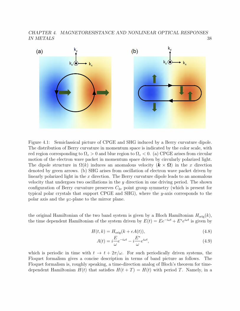
CHAPTER 4. MAGNETORESISTANCE AND NONLINEAR OPTICAL RESPONSESIN METALS 38
Figure 4.1: Semiclassical picture of CPGE and SHG induced by a Berry curvature dipole.The distribution of Berry curvature in momentum space is indicated by the color scale, withred region corresponding to Ωz > 0 and blue region to Ωz < 0. (a) CPGE arises from circularmotion of the electron wave packet in momentum space driven by circularly polarized light.The dipole structure in Ω(k) induces an anomalous velocity (k × Ω) in the x directiondenoted by green arrows. (b) SHG arises from oscillation of electron wave packet driven bylinearly polarized light in the x direction. The Berry curvature dipole leads to an anomalousvelocity that undergoes two oscillations in the y direction in one driving period. The shownconfiguration of Berry curvature preserves C2v point group symmetry (which is present fortypical polar crystals that support CPGE and SHG), where the y-axis corresponds to thepolar axis and the yz-plane to the mirror plane.
the original Hamiltonian of the two band system is given by a Bloch Hamiltonian Horig(k),the time dependent Hamiltonian of the system driven by E(t) = Ee−iωt +E∗eiωt is given by
H(t, k) = Horig(k + eA(t)), (4.8)
A(t) = iE
ωe−iωt − iE
∗
ωeiωt, (4.9)
which is periodic in time with t → t + 2π/ω. For such periodically driven systems, theFloquet formalism gives a concise description in terms of band picture as follows. TheFloquet formalism is, roughly speaking, a time-direction analog of Bloch’s theorem for time-dependent Hamiltonian H(t) that satisfies H(t + T ) = H(t) with period T . Namely, in a

CHAPTER 4. MAGNETORESISTANCE AND NONLINEAR OPTICAL RESPONSESIN METALS 39
similar manner to Bloch’s theorem, the solution for the time-periodic Schrodinger equation,
i~∂ψ(t)
∂t= H(t)ψ(t), (4.10)
is given by a time-periodic form
ψ(t) = e−iεt/~φ(t), φ(t+ T ) = φ(t), (4.11)
with the quasienergy ε. By using the time-periodic part of the wave function φ(t), thetime-dependent Schrodinger equation is rewritten as
(i~∂t + ε)φ(t) = H(t)φ(t). (4.12)
Since φ(t) is periodic in time, we can perform Fourier transformation of the both sides with
φ(t) =∑m
e−imωtφm, (4.13)
and obtain
(m~ω + ε)φm = Hmnφn, (4.14)
Hmn =1
T
∫ T
0
dtei(m−n)ωtH(t). (4.15)
Here Hmn is time-independent, but has an additional matrix structure spanned by Floquetindices m and n. Thus the time-dependent Schrodinger equation effectively reduces to atime-independent one in the Floquet formalism as,
HFφ = εφ, (4.16)
where the Floquet Hamiltonian is given by
(HF )mn =1
T
∫ T
0
dtei(m−n)ωtH(t)− n~ωδmn. (4.17)
Floquet bands obtained by diagonalizing the Floquet Hamiltonian HF offer a concise un-derstanding of the dynamics of a driven system in terms of an effective band picture. Wenote that the energy spectrum of ε shows a periodic structure with ~ω as a consequence oftranslation symmetry with respect to the Floquet index n. Thus the quasienergy spectrumis essentially described within the range −~ω/2 ≤ ε < ~ω/2, which is an analog of “the firstBrillouin zone” in Bloch’s theorem.
Since we consider the case of driving frequency much lower than the band gap, we canobtain the current expectation value by studying the Floquet band that is connected to

CHAPTER 4. MAGNETORESISTANCE AND NONLINEAR OPTICAL RESPONSESIN METALS 40
the valence band in the undriven system. In order to do so, we use standard second orderperturbation theory for
HF = H0 +H1 +H2, (4.18)
whereHi represents a term in the Floquet Hamiltonian proportional toAi. The wave functionup to the second order in A reads
|ψn〉 = |n〉 −∑m 6=n
(H1)mnEm − En
|m〉
∑m6=n
[− (H2)mnEm − En
− (H1)mn(H1)nn(Em − En)2
+∑k 6=n
(H1)mk(H1)kn(Em − En)(Ek − En)
]|m〉, (4.19)
where H0|n〉 = En|n〉. By applying the above formula to the Floquet Hamiltonian HF , weobtain Floquet states |ψ〉 that describes the steady state under the drive of incident light.The current responses in the steady state are obtained from perturbed Floquet states thatare connected to the original valence bands. This treatment can be justified when the fre-quency of incident light is much smaller than the energy difference of valence and conductionbands. (When ω satisfies conditions for optical resonances, Floquet bands originating fromvalence and conduction bands anticross each other. In this case, we cannot naively deter-mine occupation of resulting Floquet bands, which requires considering the coupling to aheat bath [52].)
By using the Floquet state |ψ〉 connected to the valence band, the time dependent currentin the steady state is given by
Jα(t) =∑m,n
tr[|ψ〉〈ψ|vα]mne−i(m−n)ωt, (4.20)
where tr denotes the trace over the band index, m,n are Floquet indices, and vα is thecurrent operator along the α-direction is given by
(vα)mn =1
T
∫ T
0
dtei(m−n)ωt∂H(t)
∂kα. (4.21)
In the following, we derive representative components of nonlinear response tensor describingCPGE and SHG by using the above method.
To study CPGE we consider a system subjected to the left circularly polarized light inthe xy plane, where the electric field is given by
E(t) = E(ex + iey)e−iωt + E∗(ex − iey)eiωt. (4.22)

CHAPTER 4. MAGNETORESISTANCE AND NONLINEAR OPTICAL RESPONSESIN METALS 41
In this case, the Floquet Hamiltonian is written as
HF = H0 +H1, (4.23)
(H0)mn =
(εv − nω 0
0 εc − nω
)δmn, (4.24)
(H1)mn = −iA∗(vx − ivy)δmn−1 + iA(vx + ivy)δmn+1, (4.25)
where εv/c is energy of valence/conduction band, vi = ∂H0/∂ki is the velocity operator forthe static Hamiltonian, A = E/ω, and we set e = 1, ~ = 1 for simplicity. Here we droppedthe term H2 proportional to A2 because it does not contribute to dc photocurrent which isproportional to AA∗ and does not involve A2 terms in the end. Since we are interested in thesecond order nonlinear current responses, it is sufficient to consider the Floquet Hamiltonianwith n = −2, . . . , 2 by starting with the unperturbed wave function |ψini〉 = |uv,n=0〉. Nowwe study dc current in the x-direction induced by circularly polarized light for the steadystate described by the Floquet state in Eq. (4.19). The velocity operator in the x-directionis written up to linear order in A as
vx = vxδmn − iA∗∂kx(vx − ivy)δmn−1
+ iA∂kx(vx + ivy)δmn+1. (4.26)
By using Eq. (4.20), we obtain the CPGE photocurrent Jx =∫
[dk]j(0)x as
j(0)x =
∑n
tr[|ψ〉〈ψ|vx]nn
= 4|E|2
ω
Im[(∂kxvx)vc(vy)cv + (vx)vc(∂kxvy)cv]
(εv − εc)2
− 3Im[(vx)vc(vy)cv][(vx)vv − (vx)cc]
(εv − εc)3
, (4.27)
where we dropped higher order terms with respect to ω by focusing on the current responsein the low frequency limit. We note that the contributions proportional to |E|2/ω2 vanishdue to the time reversal symmetry (e.g., the TRS T = K constrains Re[v] and Im[v] to beodd and even functions of k, respectively), which is used when going from the first line tothe second line. In the case of two band models, the Berry curvature is written as
Ωz = −2Im[(vx)vc(vy)cv]
(εv − εc)2, (4.28)
and the matrix elements of ∂kivj can be rewritten as
(∂kivj)vc = ∂ki [(vj)vc] + (vj)vc [i(ai)v − i(ai)c]
CHAPTER 4. MAGNETORESISTANCE AND NONLINEAR OPTICAL RESPONSESIN METALS 42
+ (vi)vc(vj)vv − (vj)cc
εv − εc, (4.29)
with (ai)v/c = 〈uv/c|∂ki |uv/c〉. By using these formulas, the CPGE photocurrent can befurther reduced as
j(0)x = 4
|E|2
ω
∂
∂kx
[Im[(vx)vc(vy)cv]
(εv − εc)2
]= −2
|E|2
ω∂kxΩz. (4.30)
The nonlinear conductivity tensor is obtained by equating the above expression and jx interms of σ and E(t) [in Eq. (4.22)] given by
jx = −iσxxy|E|2 + iσxyx|E|2 = −2iσxxy|E|2. (4.31)
Here we used antisymmetry of imaginary part of σ with respect to the last two indices. Thisleads to
σxxy =1
iω
∫[dk]∂kxΩz, (4.32)
and reproduces the semiclassical formula for σxxy in Eq. (4.7). We note that the factorτ/(1− iωτ) in the semiclassical formula [Eq. (4.7)] is replaced by the factor i/ω in the aboveformula because the τ →∞ limit (clean limit) is effectively taken in the Floquet perturbationtheory.
Next we study SHG by using Floquet perturbation theory and the two band model ina similar manner to CPGE. We consider a system driven by linearly polarized light in thex direction as Ex(t) = Ee−iωt + E∗eiωt and the SHG in the y direction. The correspondingFloquet Hamiltonian is given by
HF = H0 +H1 +H2, (4.33)
(H0)mn =
(εv − nω 0
0 εc − nω
)δmn, (4.34)
(H1)mn = (−iA∗δmn−1 + iAδmn+1) vx, (4.35)
(H2)mn =
(−(A∗)2
2δmn−2 + |A|2δmn −
A2
2δmn+2
)∂kxvx. (4.36)
We take |ψini〉 = |uv,n=0〉 as the unperturbed wave function and keep the part of the FloquetHamiltonian within the range n = −2, . . . , 2. The velocity operator along the y-direction isgiven by
vy = vyδmn + (−iA∗δmn−1 + iAδmn+1) ∂kxvy
+
(−(A∗)2
2δmn−2 + |A|2δmn −
A2
2δmn+2
)∂2kxvy. (4.37)

CHAPTER 4. MAGNETORESISTANCE AND NONLINEAR OPTICAL RESPONSESIN METALS 43
By using Eq. (4.20), we obtain the Fourier component of the current Jy =∫
[dk]jy propor-tional to e−2iωt as
j(2ω)y =
∑n
tr[|ψ〉〈ψ|vy]n+2,n
= −2iE2
iω
∂
∂kx
[Im[(vx)vc(vy)cv]
(εv − εc)2
]= i
E2
ω∂kxΩz. (4.38)
Here we again used the fact that the contributions proportional to E2/ω2 vanish due to thetime reversal symmetry, and also dropped contributions with higher powers of ω. The aboveexpression indicates that the nonlinear conductivity tensor σyxx is written as
σyxx =i
ω
∫[dk]∂kxΩz. (4.39)
This again reproduces the semiclassical formula for σyxx in Eq. (4.7).We can extend the above analysis based on the Floquet formalism to general cases with
many bands and obtain the same Berry curvature dipole formula. We sketch the derivationin the following (for details, see supplemental materials 4.5). We consider the general FloquetHamiltonian under the light irradiation which is given by
HF = H0 +H1 +H2, (4.40)
with
H1 =∑i
Aivi, H2 =1
2
∑i,j
AiAj∂kivj, (4.41)
where H0 represents a static Hamiltonian with many bands. By using the Floquet pertur-bation theory in Eq. (4.19) and the expression for the current in Eq. (4.20), we obtain thegeneral expression for the nonlinear current response as
Jr =−∑i,j
AiAj
∫[dk]
×[∑n,g
[f(εn)− f(εg)]
(1
2
(vr)ng(∂kivj)gnεn − (εg + 2ω)
+(∂rvj)ng(vi)gnεn − (εg + ω)
)+∑n,g,m
( f(εn)
εn − εm − ω− f(εg)
εg − εm + ω
)(vr)ng(vi)gm(vj)mnεn − (εg + 2ω)
+∑n,g,m
f(εn)(vj)nm(vr)mg(vi)gn
(εn − (εg + ω))(εn − (εm − ω))
+∑n
1
2f(εn)(∂kr∂kivj)nn
],
(4.42)

CHAPTER 4. MAGNETORESISTANCE AND NONLINEAR OPTICAL RESPONSESIN METALS 44
with Fermi distribution function f(ε) [where f(εn) = 1(0) for occupied (unoccupied) states]. When we expand the current Jr with respect to ω, the lowest order contribution in ω isproportional to ωA2 in the presence of time reversal symmetry. In the case of many bands,the Berry curvature dipole for the nth band is written as
∂kiΩz,n = −2Im
[〈n|∂kxH|m〉〈m|∂kyH|n〉
(εn − εm)2
], (4.43)
where n runs over occupied bands and m runs over unoccupied bands. By using this ex-pression for the Berry curvature dipole, it turns out that the lowest order contribution of Jyproportional to ωA2 is written as
Jy = −iwA2x
∫[dk]f(εn)∂kxΩz,n, (4.44)
which reproduces the Berry curvature dipole formula Eq. (4.7) for SHG in the case of manybands. Details of the above calculation for many band cases are described in Appendix 4.5.
To summarize, we derived formulas for CPGE and SHG in the sufficiently low frequencyregion in a fully quantum mechanical way by using Floquet perturbation theory. This re-produces the semiclassical formula with Berry curvature dipole.
4.3 Semiclassical formulas for magnetoconductance
We apply SCA to obtain semiclassical formula for nonlinear magneto-conductivity that in-cludes all terms proportional to B2E is applicable to Weyl semimetals and may explain direc-tional anisotropy of magnetoconductivity of Weyl semimetals recently reported in Ref. [46,78], which we perform in Sec. 4.4. Third, TR symmetric Weyl semimetals can support largenonlinear Kerr rotation. Intraband contribution to SHG vanishes for B = 0 in TR symmetricWeyl semimetals, and the SHG signal has a contribution linear in B. Thus application of Bmay lead to giant nonlinear Kerr rotation.
We derive semiclassical formulas for nonlinear magneto-optical effects up to the secondorder in E. It is convenient to rewrite the equations of motion (4.1) to collect time derivativeson the left:
r =1
~D[∇kεk + eE ×Ωk +
e
~(∇kεk ·Ωk)B], (4.45)
~k =1
D[−eE − e
~∇kεk ×B −
e2
~(E ·B)Ωk], (4.46)
D = 1 +e
~B ·Ωk. (4.47)
The charge density ρ and current density j are given by
ρ = −e∫
[dk]Df, (4.48)

CHAPTER 4. MAGNETORESISTANCE AND NONLINEAR OPTICAL RESPONSESIN METALS 45
j = −e∫
[dk](Dr + ∇r ×mk)f, (4.49)
with [dk] = dk/(2π)3, where the second term of j is a contribution of magnetization current.We note that the factor D arises from a field-induced change of the volume of the phase space[77]. In the following, we focus on the uniform system. In this case, the expression of thecurrent density reduces to
j = −e∫
[dk][vk +e
~E ×Ωk +
e
~(vk ·Ωk)B]f, (4.50)
where we used
vp = vk − (1/~)∇k(m ·B), (4.51)
with vk = (1/~)∇kε0k.
Now we focus on responses driven by monochromatic light with the electric field E(t) =Ee−iωt. We consider current responses at order of E. We write the distribution function inFourier components as
f = f0 + f1e−iωt, (4.52)
where f0 is the unperturbed distribution function and other terms appear in the presence ofthe electric field of the incident light. The steady-state distribution function is determinedby the Boltzmann equation
df
dt=f0 − fτ
, (4.53)
where
df
dt= k ·∇kf + ∂tf. (4.54)
In the following, we apply the above SCA to the linear current responses in the presence ofmagnetic fields.
We derive the semiclassical formula for the conductivity up to the second order of B interms of Berry curvature and orbital magnetic moment.
The current response of the frequency ω is obtained from f1 in Eq. (4.52). By equatingterms proportional to e−iωt in Eq. (4.54), we obtain
[−eE − e2
~(E ·B)Ωk] ·∇pf0 − iωf1 = −f1
τ, (4.55)
with ∇p = (1/~)∇k, where we dropped the term involving (∇kεk) ×B because it is per-pendicular to ∇pf0 = (1/~)(∇kεk)∂εf0. This leads to
f1 =−τ
1− iωτ1
D[−eE − e2
~(E ·B)Ωk] ·∇pf0. (4.56)

CHAPTER 4. MAGNETORESISTANCE AND NONLINEAR OPTICAL RESPONSESIN METALS 46
Now the current response linear in E is given by
j1 =eτ
1− iωτ
∫BZ
[dk]1
D
[vk +
e
~(vk ·Ωk)B]
× [−eE − e2
~(E ·B)Ωk] ·∇pf0 +
e
~E ×Ωkf0
, (4.57)
where f0 = θ(EF − εk − mk · B) with the step function θ(x) = 0(x < 0), 1(x ≥ 0).This expression is reduced if we focus on the case where the electric field E is appliedalong the ith direction and the system preserves the TRS in the absence of magnetic fields.Specifically, we consider terms up to ∝ B that are nonvanishing with the TRS by expandingas 1/D ' 1 + (e/~)B ·Ωk, which leads to
j1 =eτ
1− iωτ
∫BZ
[dk]−vkeE(vk)i∂εf′0
+e
~(E ×Ωk)(m ·B)∂εf
′0, (4.58)
with f ′0 = θ(EF − εk), i.e., a distribution function when B = 0. Here we used the factthat ∂pi ,vp,Ω,, and m are odd under the TRS. The first term in the integral is the metal-lic conductivity, while the second term describes regular Hall conductivity linear in B (incontrast to anomalous Hall conductivity which is nonzero in the absence of B). This secondterm indicates that the orbital magnetic moment gives a semiclassic description related toLandau level formation in the quantum limit. We note that there is no B-linear contributionto the longitudinal conductivity σii because the Onsager relation constrains the conductivityas σij(B) = σji(−B) and the longitudinal conductivity should be an even function of B.
Next, we derive the formula for the longitudinal magnetoconductance. Its lowest orderdependence on B is quadratic due to the Onsager relation. The B2 contribution to thelongitudinal current response is explicitly written as
jB2 =e2τ
~
∫BZ
[dk]− e
~E ·∇kf0(ε0)[−e(vk ·Ωk)(B ·Ωk)B− eΩk ·∇k(m ·B)B
+ e(B ·Ωk)2vk + (B ·Ωk)∇k(m ·B)] + [1
~E ·∇k(
∂f0(ε0)
∂εm ·B)
− e
~(E ·B)(Ωk ·∇kf0(ε0))][e(vk ·Ωk)B− e(B ·Ωk)vk − ∂k(m ·B)]
+e
~(E ·B)[Ωk · ∂k(
∂f0(ε0)
∂εm ·B)]vk −
1
2E · ∂k[
∂2f0(ε0)
∂ε2(m ·B)2]vk
.
(4.59)
In addition to terms that contribute isotropically to the current density, there are sev-eral terms that contribute to the current density specifically along B which results in ananisotropic magnetoconductance if it is applied to Weyl semimetals as we discuss in Sec. 4.4.

CHAPTER 4. MAGNETORESISTANCE AND NONLINEAR OPTICAL RESPONSESIN METALS 47
[ρxx(B)-ρxx(B=0)]/ρxx(B=0)
(a) Berry curvature Ω (b) Orbital magnetic moment m
(c) Interplay of Ω and m
(B 2e2/ h2k4F )
(d) Total magneto-resistance
[ρxx(B)-ρxx(B=0)]/ρxx(B=0) (B 2e2/ h2k4F )
[ρxx(B)-ρxx(B=0)]/ρxx(B=0) (B 2e2/ h2k4F ) [ρxx(B)-ρxx(B=0)]/ρxx(B=0) (B 2e2/ h2k4F )
Figure 4.2: Angle-dependence of longitudinal magnetoresistance (LMR) for Weyl semimet-als derived from the semiclassical approach [Eq. (4.59)]. Blue lines are polar plots of theLMR [ρxx(B)− ρxx(B = 0)]/ρxx(B = 0) as a function of the relative angle θ between E andB. We show angle-dependences of contributions to the LMR from (a) the Berry curvature,(b) the orbital magnetic moment, (c) the interplay between the Berry curvature and theorbital magnetic moment, and (d) the total angle-dependence of the LMR.

CHAPTER 4. MAGNETORESISTANCE AND NONLINEAR OPTICAL RESPONSESIN METALS 48
4.4 Angle-dependent magnetoresistance
In this section, we study magnetoresistance by using the SCA developed in the previous sec-tion. In particular, we focus on the current response J ∝ EB2 and study how the Berry cur-vature and the orbital magnetic moment contribute to magnetoresistance in Weyl semimetals,since the interplay of these two quantities in transport properties of Weyl semimetals hasnot been fully investigated except for a few studies [85, 47, 62, 70]. The obtained angle-dependence of magnetoresistance is compared with recent magneto-transport experimentsfor Dirac semimetals [46, 78].
We consider the Hamiltonian for Weyl semimetals given by
H = ηvFσ · p, (4.60)
where vF is the Fermi velocity and η = ±1 specifies the chirality. In this case, the velocityoperator, the Berry curvature, the orbital magnetic moment are written as
vk = vF k, (4.61)
Ω = −η 1
2k2k, (4.62)
m = −ηevF2kk, (4.63)
for the conduction band, where k denotes the unit vector along k.Now we apply the semiclassics formula Eq. (4.59) for the linear current response j1
proportional to B2 to Weyl semimetals and study the angle-dependent magnetoresistance.First, we suppose that the electric field is applied in the z-direction as E = Eez where ezdenotes the unit vector along the z direction. In this case, the current along the z-direction(j1)z is given by
(j1)z =1
6π2~τe2vFk
2FE +
1
30π2~3k2F
τe4vFB2E (4.64a)
when E ‖ B, and
(j1)z =1
6π2~τe2vFk
2FE −
1
60π2~3k2F
τe4vFB2E (4.64b)
when E ⊥ B (e.g. B ‖ x), where we assumed τω 1. Here, the first term is the isotropicdc conductivity and the second term is an anisotropic correction which originates from theE · B term related to the chiral anomaly in Weyl semimetals. The second term accountsfor the negative magnetoresistance (MR) when E ‖ B, and the positive MR when E ⊥ B.Thus the semiclassical theory for the linear conductivity including effects of both Ω andm captures the directional anisotropy of linear conductivity in the B field which is usuallyconsidered to be an evidence of a Weyl fermion in transport measurements.

CHAPTER 4. MAGNETORESISTANCE AND NONLINEAR OPTICAL RESPONSESIN METALS 49
Next, we discuss the full angle dependence of the current response in the magnetic field.When the electric field is applied in the direction tilted by θ from the direction of the magneticfield B, the longitudinal magneto conductivity σ(B) is given by
σ(B)− σ(B = 0)
σ(B = 0)=−1 + 3 cos2 θ
10
e2B2
~2k4F
. (4.65)
Equation (4.65) does not depend on the chirality of the Weyl node nor in which band thechemical potential is located. It shows that the magnetoresistance (MR) is positive whenE ⊥ B and it decreases to negative as θ → 0. If we separately look at contributions tothe MR from the Berry curvature and the orbital magnetic moment, we find that either theBerry curvature or the orbital magnetic moment alone gives a negative magnetoresistance(Figs. 4.2a and 4.2b), while the interplay between the Berry curvature and the orbital mag-netic moment gives a positive magnetoresistance (Fig. 4.2c). As a whole, Eq. (4.65) givesthe angular dependences as shown in Fig. 4.2d. We note that the anisotropic magnetocon-ductance in the semiclassics [Eq. (4.65)] is not solely described by the contribution from thechiral anomaly. Specifically, the contribution from the chiral anomaly which was discussedin Ref. [65] is found in the term
−e4τ
~
∫BZ
[dk](Ωk ·∇pf0(ε0))(vk ·Ωk)(E ·B)B (4.66)
in Eq. (4.59) and gives a negative magnetoresistance in Weyl semimetals. In contrast, thereare several terms involving the orbital magnetic moment which lead to contributions ofopposite signs.
A similar angular dependence of the magnetoresistance to Eq. (4.65) in the weak fieldregion have been observed in magneto-transport experiments of Dirac semimetals [46, 78].In particular, Ref. [78] reported that the sign change of the MR occurs around 45 in thelow B region for Dirac semimetal Na3Bi, which is consistent with our semiclassical resultshown in Fig. 4.2(d). We note that our calculation for Weyl semimetals is also applicable toDirac semimetals with a mild assumption that the degenerate energy bands having oppositechirality in Dirac semimetals are decoupled with each other.
Finally, we present estimates for the above nonlinear conductivities derived for Weylsemimetals. The directional anisotropy of the linear conductivity is given by the ratio of thetwo terms ∝ B0 and ∝ B2 in Eq. (4.64). The anisotropy ratio amounts to 0.06(B/1 T)2 fortypical parameters vF = 3× 10⁵ m/s, EF = 10 meV for the Weyl semimetal material, TaAs[73, 39].
4.5 Supplemental material for derivation of the Berry
curvature dipole formula for general bands
In this appendix, we apply the Floquet perturbation theory to systems with a general numberof bands and derive the formula for SHG in terms of Berry curvature dipole. The derivation

CHAPTER 4. MAGNETORESISTANCE AND NONLINEAR OPTICAL RESPONSESIN METALS 50
proceeds in a similar manner to the two band case presented in Sec. 4.2B, but with involvingmore band indices.
We consider the system irradiated with monochromatic light which is described by thetime-dependent Hamiltonian,
H(t) = H(p+ eA(t)) = H0 +H1 +H2 + · · ·
= H +∑i
(∂kiH)eAie−iωt +
∑i,j
1
2(∂ki∂kjH)e2AiAje
−2iωt + · · · , (4.67)
where H0 ≡ H is the static Hamiltonian in the absence of the driving, and A(t) = Ae−iωt
is the vector potential. For the time periodic Hamiltonian H(t), the Floquet Hamiltonian isdefined by
(HF )mn =1
T
∫ T
0
dtei(m−n)ΩtH(t)− n~Ωδmn, (4.68)
with Floquet indices m an n. In the following, we adopt a simplified notation where we writecontributions H i(t) to the Floquet Hamiltonian HF just by H i.
The standard perturbation theory gives the wave function for the perturbed FloquetHamiltonian HF as
|ψn〉 = |n〉+∑g 6=n
H1gn
εn − εg|g〉+
∑n6=mg 6=n
[H1gmH
1mn
(εn − εm)(εn − εg)−
H1nnH
1gn
(εn − εg)2+
H2gn
εn − εg
]|g〉, (4.69)
where |n〉 is the unperturbed wave function satisfying H|n〉 = εn|n〉, and n labels the set ofthe band index and the Floquet index. Here we note that H1
nn = 0 in the present case. Theexplicit form of the wave function ψn with the band index n and any Floquet index (say, 0)is given by
|ψn〉 =|n〉+ e∑n,g
(∂kiHAi)gnεn − (εg + ω)
|g〉+1
2e2∑n,g
(∂ki∂kjHAiAj)gn
εn − (εg + 2ω)|g〉
+ e2∑n,m,g
[(∂kjHAj)gm(∂kiHAi)mn
(εn − (εm + ω))(εn − (εg + 2ω))
]|g〉 , (4.70)
where |n〉 denotes the static wave function with the band index n, εn denotes the staticenergy dispersion with the band index n, and Om,n = 〈m|O|n〉.
Now we consider the current response in the α-direction is given by
Jα(t) = −e∑n
f(εn)∑m′,n′
tr[|ψ(n,0)〉〈ψ(n,0)|vα]m′n′e−i(m′−n′)ωt, (4.71)
where |ψ(n,0)〉 is the perturbed wave function with the band index n and the Floquet index0, and m′, n′ denote the Floquet indices. The Fermi distribution function f(ε) is given

CHAPTER 4. MAGNETORESISTANCE AND NONLINEAR OPTICAL RESPONSESIN METALS 51
by f(εn) = 1 for occupied bands and f(εn) = 0 for unoccupied bands. Since we considerthe low-frequency limit where optical transition does not take place, we can assume thatthe occupation of the perturbed states coincides with that of the unperturbed states. Theoperator v is Floquet representation of the time-dependent velocity operator v(t) which isgiven by
(vi)m′n′ =1
T
∫ T
0
dtei(m′−n′)ωtvi(t) (4.72)
vi(t) = v0i + v1
i + v2i + · · ·
= ∂kiH +∑j
(∂ki∂kjH)eAje−iωt +
∑i,j
1
2(∂ki∂kj∂klH)e2AjAle
−2iωt + · · · . (4.73)
For the real external field A(t) = Ae−iωt + Aeiωt, we obtain the second-order currentresponse Jr along the r-direction which is proportional to e−i2ωt as
Jr = −e3∑i,j
AiAj
∫[dk]
∑n,g
[1
2f(εn)
(∂ki∂kjH)gn
εn − (εg + 2ω)〈n|∂krH|g〉
+1
2f(εn)
(∂ki∂kjH)ng
εn − (εg − 2ω)〈g|∂krH|n〉
+∑m
f(εn)
εn − εm − ω(∂kjH)gm(∂kiH)mn
εn − (εg + 2ω)〈n|∂krH|g〉
+∑m
f(εn)
εn − εm + ω
(∂kiH)nm(∂kjH)mg
εn − (εg − 2ω)〈g|∂krH|n〉
+f(εn)(∂kiH)gn
εn − (εg + ω)〈n|∂kr∂kjH|g〉+ f(εn)
(∂kiH)ngεn − (εg − ω)
〈g|∂kr∂kjH|n〉
+∑m
f(εn)(∂kiH)gn
εn − (εg + ω)
(∂kjH)nm
εn − (εm − ω)〈m|∂krH|g〉+
1
2f(εn)〈n|∂kr∂ki∂kjH|n〉
].
(4.74)This expression can be rewritten as
Jr = −e3∑i,j
AiAj
∫[dk]
∑n
[∑g
1
2(f(εn)− f(εg))
〈n|∂krH|g〉〈g|∂ki∂kjH|n〉εn − (εg + 2ω)
+∑m,g
( f(εn)
εn − εm − ω− f(εg)
εg − εm + ω
)〈n|∂krH|g〉〈g|∂kiH|m〉〈m|∂kjH|n〉εn − (εg + 2ω)
+∑g
(f(εn)− f(εg))〈n|∂kr∂kjH|g〉〈g|∂kiH|n〉
εn − (εg + ω)
+∑m,g
f(εn)〈n|∂kjH|m〉〈m|∂krH|g〉〈g|∂kiH|n〉
(εn − (εg + ω))(εn − (εm − ω))+
1
2f(εn)〈n|∂kr∂ki∂kjH|n〉
].

CHAPTER 4. MAGNETORESISTANCE AND NONLINEAR OPTICAL RESPONSESIN METALS 52
(4.75)
Since we are interested in the intraband effects in the low frequency limit (ω much smallerthan the bandgap), we expand the current Jr in terms of ω as Jr = J0
r + J1r + J2
r + . . ., withJnr ∝ ωn . The lowest order term in ω is the zeroth order term which is given by
J0r = −e3
∑i,j
AiAj
∫[dk]
∑n
[∑g
1
2(f(εn)− f(εg))
〈n|∂krH|g〉〈g|∂ki∂kjH|n〉εn − εg
+′∑
m,g
( f(εn)
εn − εm− f(εg)
εg − εm
)〈n|∂krH|g〉〈g|∂kiH|m〉〈m|∂kjH|n〉εn − εg
+′∑g
(f(εn)− f(εg))〈n|∂kr∂kjH|g〉〈g|∂kiH|n〉
εn − εg
+′∑
m,g
f(εn)〈n|∂kjH|m〉〈m|∂krH|g〉〈g|∂kiH|n〉
(εn − εg)(εn − εm)
−2′∑g
f(εn)〈n|∂krH|g〉〈g|∂kiH|n〉〈n|∂kjH|n〉
(εn − εg)2
−2′∑g
f(εg)〈n|∂krH|g〉〈g|∂kiH|g〉〈g|∂kjH|n〉
(εn − εg)2
+′∑m
f(εn)〈n|∂kjH|m〉〈m|∂krH|n〉〈n|∂kiH|n〉
(εn − εm)2
+′∑g
f(εn)〈n|∂kjH|n〉〈n|∂krH|g〉〈g|∂kiH|n〉
(εn − εg)2+
1
2e2f(εn)〈n|∂kr∂ki∂kjH|n〉
].
(4.76)
Here∑′
g (∑′
m,g) denotes the summation where the band index g (m, g) runs over those thatdo not set the denominator to zero. We note that the 5th to 8th terms are obtained bysetting one energy denominator to be 1/ω and expanding the other energy denominator upto ω2 in the 2nd and the 4th terms in Eq. (4.75). In addition, the time reversal symmetry,T = K, leads to the symmetry properties of the Hamiltonian and its eigenstates given by
H(k) = H(−k), ε(k) = ε(−k), |n(k)〉 = 〈n(−k)|. (4.77)
By using these properties that hold in the presence of the time-reversal symmetry, we findthat the above expression for J0
r vanishes in the zeroth order. Therefore, the lowest orderterm is actually the first order term J1
r .The first order term in ω is written as
Jr = −e3ω∑i,j
AiAj
∫[dk]
∑n
[ ′∑g
(f(εn)− f(εg))〈n|∂krH|g〉〈g|∂ki∂kjH|n〉
(εn − εg)2
CHAPTER 4. MAGNETORESISTANCE AND NONLINEAR OPTICAL RESPONSESIN METALS 53
+2′∑
m,g
(f(εn)
εn − εm− f(εg)
εg − εm
) 〈n|∂krH|g〉〈g|∂kiH|m〉〈m|∂kjH|n〉(εn − εg)2
+′∑
m,g
(f(εn)
(εn − εm)2+
f(εg)
(εg − εm)2
) 〈n|∂krH|g〉〈g|∂kiH|m〉〈m|∂kjH|n〉εn − εg
−4′∑g
f(εn)〈n|∂krH|g〉〈g|∂kiH|n〉〈n|∂kjH|n〉
(εn − εg)3
−4′∑g
f(εg)〈n|∂krH|g〉〈g|∂kiH|g〉〈g|∂kjH|n〉
(εn − εg)3
+′∑g
(f(εn)− f(εg))〈n|∂kr∂kjH|g〉〈g|∂kiH|n〉
(εn − εg)2
−′∑m
f(εn)〈n|∂kjH|m〉〈m|∂krH|n〉〈n|∂kiH|n〉
(εn − εm)3
+′∑g
f(εn)〈n|∂kjH|n〉〈n|∂krH|g〉〈g|∂kiH|n〉
(εn − εg)3
−′∑
m,g
f(εn)〈n|∂kjH|m〉〈m|∂krH|g〉〈g|∂kiH|n〉
(εn − εg)(εn − εm)2
+′∑
m,g
f(εn)〈n|∂kjH|m〉〈m|∂krH|g〉〈g|∂kiH|n〉
(εn − εg)2(εn − εm)
]. (4.78)
By using the properties from the time reversal symmetry, this can be reduced as
Jr = −2e3ω∑i,j
AiAj
∫[dk]
∑n
f(εn)
[ ′∑g
f(εn)〈n|∂krH|g〉〈g|∂ki∂kjH|n〉
(εn − εg)2
+2′∑
m,g
1
εn − εm〈n|∂krH|g〉〈g|∂kiH|m〉〈m|∂kjH|n〉
(εn − εg)2
+′∑
m,g
1
(εn − εm)2
〈n|∂krH|g〉〈g|∂kiH|m〉〈m|∂kjH|n〉εn − εg
−3′∑g
〈n|∂krH|g〉〈g|∂kiH|n〉〈n|∂kjH|n〉(εn − εg)3
+′∑g
〈n|∂kr∂kjH|g〉〈g|∂kiH|n〉(εn − εg)2
−′∑
m,g
〈n|∂kjH|m〉〈m|∂krH|g〉〈g|∂kiH|n〉(εn − εg)(εn − εm)2
]. (4.79)
CHAPTER 4. MAGNETORESISTANCE AND NONLINEAR OPTICAL RESPONSESIN METALS 54
Now let us consider the specific case relevant to the Berry curvature dipole formula.Namely we suppose that E is applied along the x-direction and consider the current J inthe y-direction:
Jy = −2e3ωAxAx
∫[dk]
∑n
f(εn)
[ ′∑g
f(εn)〈n|∂kyH|g〉〈g|∂kx∂kxH|n〉
(εn − εg)2
+2′∑
m,g
1
εn − εm〈n|∂kyH|g〉〈g|∂kxH|m〉〈m|∂kxH|n〉
(εn − εg)2
−3′∑g
〈n|∂kyH|g〉〈g|∂kxH|n〉〈n|∂kxH|n〉(εn − εg)3
+′∑
m,g
1
(εn − εm)2
〈n|∂kyH|g〉〈g|∂kxH|m〉〈m|∂kxH|n〉εn − εg
+′∑g
〈n|∂ky∂kxH|g〉〈g|∂kxH|n〉(εn − εg)2
−′∑
m,g
〈n|∂kxH|m〉〈m|∂kyH|g〉〈g|∂kxH|n〉(εn − εg)(εn − εm)2
]. (4.80)
The k-integral of the Berry curvature dipole Ωz,n for the nth band is explicitly written inmany band systems as∫
[dk] ∂xΩz,n(k) = −2∂x
∫[dk] Im[〈∂xn|∂yn〉]
= i∂x
∫[dk]
∑g
[〈∂xn|g〉〈g|∂yn〉 − 〈∂yn|g〉〈g|∂xn〉]
= i∂x
∫[dk]
′∑g
[〈n|∂xH|g〉〈g|∂yH|n〉
(εn − εg)2− 〈n|∂yH|g〉〈g|∂xH|n〉
(εn − εg)2
]
= −2i
∫[dk]
′∑g
[〈n|∂yH|g〉〈∂xg|∂xH|n〉
(εn − εg)2+〈n|∂yH|g〉〈g|∂x∂xH|n〉
(εn − εg)2
+〈n|∂yH|g〉〈g|∂xH|∂xn〉
(εn − εg)2+〈∂xn|∂yH|g〉〈g|∂xH|n〉
(εn − εg)2
+〈n|∂x∂yH|g〉〈g|∂xH|n〉
(εn − εg)2+〈n|∂yH|∂xg〉〈g|∂xH|n〉
(εn − εg)2
− 2〈n|∂yH|g〉〈g|∂xH|n〉
(εn − εg)3[(vx)nn − (vx)gg]
]= −2i
∫[dk]
′∑g
[〈n|∂yH|g〉〈g|∂x∂xH|n〉
(εn − εg)2+〈n|∂x∂yH|g〉〈g|∂xH|n〉
(εn − εg)2
− 2〈n|∂yH|g〉〈g|∂xH|n〉
(εn − εg)3[(vx)nn − (vx)gg]
]
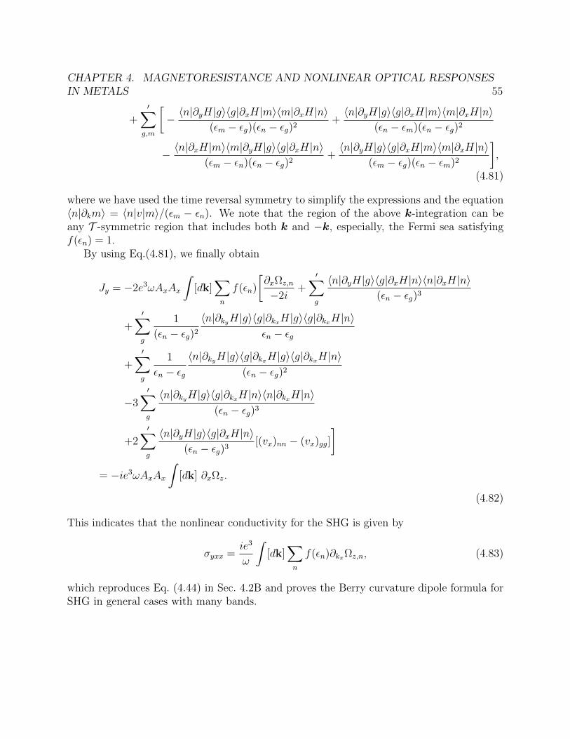
CHAPTER 4. MAGNETORESISTANCE AND NONLINEAR OPTICAL RESPONSESIN METALS 55
+′∑
g,m
[− 〈n|∂yH|g〉〈g|∂xH|m〉〈m|∂xH|n〉
(εm − εg)(εn − εg)2+〈n|∂yH|g〉〈g|∂xH|m〉〈m|∂xH|n〉
(εn − εm)(εn − εg)2
− 〈n|∂xH|m〉〈m|∂yH|g〉〈g|∂xH|n〉(εm − εn)(εn − εg)2
+〈n|∂yH|g〉〈g|∂xH|m〉〈m|∂xH|n〉
(εm − εg)(εn − εm)2
],
(4.81)
where we have used the time reversal symmetry to simplify the expressions and the equation〈n|∂km〉 = 〈n|v|m〉/(εm − εn). We note that the region of the above k-integration can beany T -symmetric region that includes both k and −k, especially, the Fermi sea satisfyingf(εn) = 1.
By using Eq.(4.81), we finally obtain
Jy = −2e3ωAxAx
∫[dk]
∑n
f(εn)
[∂xΩz,n
−2i+
′∑g
〈n|∂yH|g〉〈g|∂xH|n〉〈n|∂xH|n〉(εn − εg)3
+′∑g
1
(εn − εg)2
〈n|∂kyH|g〉〈g|∂kxH|g〉〈g|∂kxH|n〉εn − εg
+′∑g
1
εn − εg〈n|∂kyH|g〉〈g|∂kxH|g〉〈g|∂kxH|n〉
(εn − εg)2
−3′∑g
〈n|∂kyH|g〉〈g|∂kxH|n〉〈n|∂kxH|n〉(εn − εg)3
+2′∑g
〈n|∂yH|g〉〈g|∂xH|n〉(εn − εg)3
[(vx)nn − (vx)gg]
]= −ie3ωAxAx
∫[dk] ∂xΩz.
(4.82)
This indicates that the nonlinear conductivity for the SHG is given by
σyxx =ie3
ω
∫[dk]
∑n
f(εn)∂kxΩz,n, (4.83)
which reproduces Eq. (4.44) in Sec. 4.2B and proves the Berry curvature dipole formula forSHG in general cases with many bands.

56
Chapter 5
Hall conductivity in aninhomogeneous electric field
In this chapter we will study the Hall conductivity of insulators in a static inhomogeneouselectric field to the second order of wave number q using the Kubo formula. We derivegeneral formulas for the q2 term in hall conductivity. We find that for an insulator with onlytwo bands that are flat, the q2 term is determined by the quantum metric tensor and theBerry curvature. Using a semiclassical derivation we provide an intuitive picture of how thequantum metric tensor appears. We end this chapter with numerical studies on a topologicalflat band model and the Hofstadter model.
5.1 Preliminaries and background
Strain tensor [45]Under deformation the position x of a point in a solid body will bemapped to a new position x′. We use Euclidean coordinates xi to label the originalposition of the point and the deformation will be equivalent to a change of the metric of thecoordinate system. In the new Euclidean coordinate system the distance between two veryclose points will be
dl′2 =∑i
dx′2i =∑i
(∂x′i∂xj
dxj)2 =
∑i
∂x′i∂xj
∂x′i∂xk
dxjdxk . (5.1)
We can rewrite it in terms of the displacement of the point ui = x′i − xi,
dl′2 = dl2 + 2uikdxidxk (5.2)
where uik = 12
( ∂ui∂xk
+ ∂uk∂xi
+ ∂ul∂xi
∂ul∂xk
) is the strain tensor. Usually the deformation we consideris very small so we can neglect the last term in the strain tensor uik and have
uik =1
2
(∂ui∂xk
+∂uk∂xi
)(5.3)

CHAPTER 5. HALL CONDUCTIVITY IN AN INHOMOGENEOUS ELECTRICFIELD 57
Stress tensor When deformation occurs forces will arise as they would like to make thesystem return to equilibrium. These forces are called internal stresses and in our assumptionthey have very short range of action.
Let’s consider one component of the total force caused by deformation on some portionof the system. It will be given by ∫
Fi(~x)dV (5.4)
where the integral is taken over the volume of that portion of the body. Since the stress isshort range and hence can only act on the surface of the body, the integral should be ableto be rewritten as an integral over a surface. Therefore, there must exist a tensor σik suchthat Fi is given by
Fi =∂σik∂xk
. (5.5)
The tensor σik here is called the stress tensor.
Viscosity The deformation of a body will be reversible if it occurs with an infinitesimalspeed so that the thermodynamic equilibrium is established at every moment. In the processof realistic deformation if there is any internal motion in the body, there will be irreversibleprocesses arising from the finite velocity of that motion. The irreversible processes will thenlead to energy dissipation. This means of dissipation is called viscosity.
It is clear that the forces in the irreversible process should relate to the velocity of thedeformation. In addition, it should meet the requirement that when the motion of the systemis a general translation or rotation the forces should be zero as there is no internal motion.It turns out that the dissipation can be described by the time derivative of the strain tensorµ.
Including the forces from viscosity the stress tensor will be given by
σαβ = λαβγδµγδ − ηαβγδµγδ (5.6)
where the first coefficient is called elastic modulus and the second is the viscosity tensor.
Odd viscosity In general, the viscosity tensor need not to be symmetric. Actually onethe symmetric part of the viscosity tensor describes the dissipation while the antisymmetricpart is not associated with dissipation. We call the antisymmetric part odd viscosity and itvanishes if there is time reversal symmetry according to Onsager relation.
ηS(B) =ηS(−B)
ηA(B) =− ηA(−B)(5.7)
In two dimensions, ηA has three independent coefficients ηA1112, ηA1122, η
A1222. In an isotropic
system we haveηA1112 = ηA1222 = η, ηA1122 = 0 . (5.8)

CHAPTER 5. HALL CONDUCTIVITY IN AN INHOMOGENEOUS ELECTRICFIELD 58
Hall viscosity Quantum fluids have a ground state with a finite gap. At zero temperaturethey have nondissipative responses so we will have ηS = 0 while ηA may or may not be zero.
We now consider a family of Hamiltonians H(uαβ) which depends smoothly on uαβ.According to the adiabatic response theory, in a uniform deformation we will have [8]⟨
∂H
∂uαβ
⟩=
∂ε
∂uαβ+∑λδ
Ωαβλδuλδ . (5.9)
where ε is the energy of the system. The adiabatic curvature Ω is the corresponding non-dissipative (odd) viscosity tensor and it is also named as Hall viscosity.
Hall conductivity and Hall viscosity In a Galilean invariant system in which particleshave the same charge/mass ratio, it has been shown that Hall viscosity is related to the Hallconductivity in an inhomogeneous electric field [37, 15]. It is shown that in a two dimensionalquantum Hall system, the Hall conductivity tensor σxy(q) can be expanded as
σxy(q)
σxy(0)= 1 + C2(q2`2) +O(q4`4) (5.10)
where ` =√
~c/eB is the magnetic length and
C2 =ηA
~n− 2π
ν
`2
~ωcB2ε′′(B) (5.11)
where ν is the filling factor, ε is the energy density, n is the density of electrons and ωc = eBmc
isthe cyclotron frequency of the quantum Hall state. For integer quantum Hall state with ν = 1the first term gives 1
4and the second term gives −1 and in total we will have C2 = −3
4[37]. In
the following sections we will calculate the coefficient of the Hall conductivity in the secondorder in q using Kubo formula and semiclassical theory.
5.2 Derivation of the q2 term in Hall conductivity
5.2.1 Symmetry analysis
Before we do the derivation we would like to first do the symmetry analysis for the Hallconductivity tensor. We do it by looking at requirements on the dielectric tensor εij(ω,q) andusing the relation between the dielectric tensor and the Hall conductivity tensor, σij(ω,q) =iωεij(ω,q). The dielectric tensor for a non-dissipative system obeys the following threerequirements:
• Hermitian: εij(ω,q) = ε∗ji(ω,q)
• Onsager’s relation: εij(ω,q, B) = εji(ω,−q,−B)
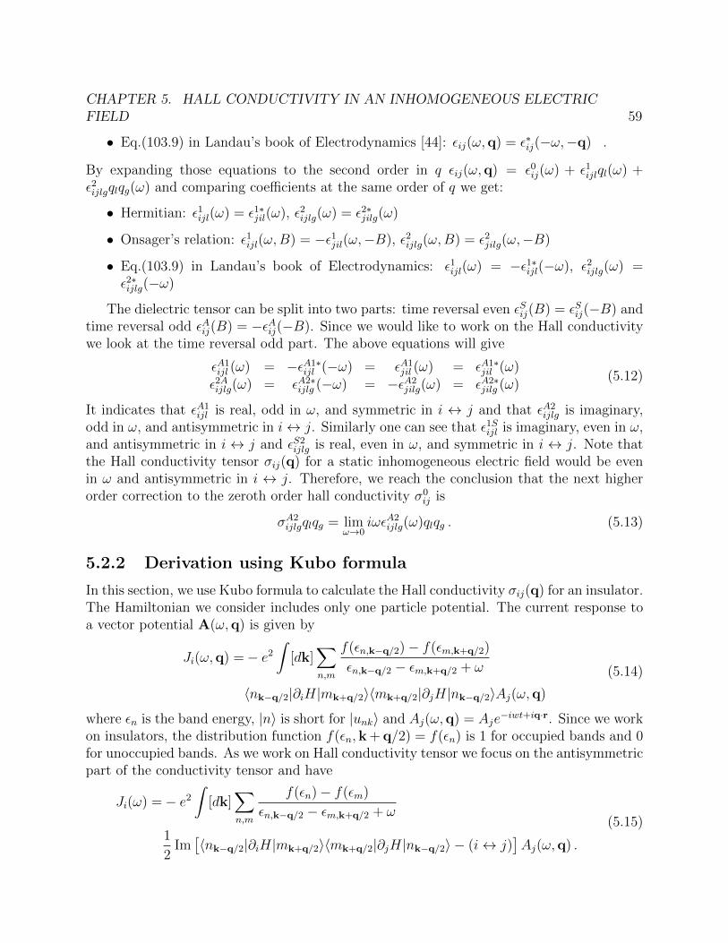
CHAPTER 5. HALL CONDUCTIVITY IN AN INHOMOGENEOUS ELECTRICFIELD 59
• Eq.(103.9) in Landau’s book of Electrodynamics [44]: εij(ω,q) = ε∗ij(−ω,−q) .
By expanding those equations to the second order in q εij(ω,q) = ε0ij(ω) + ε1ijlql(ω) +ε2ijlgqlqg(ω) and comparing coefficients at the same order of q we get:
• Hermitian: ε1ijl(ω) = ε1∗jil(ω), ε2ijlg(ω) = ε2∗jilg(ω)
• Onsager’s relation: ε1ijl(ω,B) = −ε1jil(ω,−B), ε2ijlg(ω,B) = ε2jilg(ω,−B)
• Eq.(103.9) in Landau’s book of Electrodynamics: ε1ijl(ω) = −ε1∗ijl(−ω), ε2ijlg(ω) =ε2∗ijlg(−ω)
The dielectric tensor can be split into two parts: time reversal even εSij(B) = εSij(−B) andtime reversal odd εAij(B) = −εAij(−B). Since we would like to work on the Hall conductivitywe look at the time reversal odd part. The above equations will give
εA1ijl (ω) = −εA1∗
ijl (−ω) = εA1jil (ω) = εA1∗
jil (ω)ε2Aijlg(ω) = εA2∗
ijlg (−ω) = −εA2jilg(ω) = εA2∗
jilg (ω)(5.12)
It indicates that εA1ijl is real, odd in ω, and symmetric in i ↔ j and that εA2
ijlg is imaginary,odd in ω, and antisymmetric in i↔ j. Similarly one can see that ε1Sijl is imaginary, even in ω,and antisymmetric in i ↔ j and εS2
ijlg is real, even in ω, and symmetric in i ↔ j. Note thatthe Hall conductivity tensor σij(q) for a static inhomogeneous electric field would be evenin ω and antisymmetric in i ↔ j. Therefore, we reach the conclusion that the next higherorder correction to the zeroth order hall conductivity σ0
ij is
σA2ijlgqlqg = lim
ω→0iωεA2
ijlg(ω)qlqg . (5.13)
5.2.2 Derivation using Kubo formula
In this section, we use Kubo formula to calculate the Hall conductivity σij(q) for an insulator.The Hamiltonian we consider includes only one particle potential. The current response toa vector potential A(ω,q) is given by
Ji(ω,q) =− e2
∫[dk]
∑n,m
f(εn,k−q/2)− f(εm,k+q/2)
εn,k−q/2 − εm,k+q/2 + ω
〈nk−q/2|∂iH|mk+q/2〉〈mk+q/2|∂jH|nk−q/2〉Aj(ω,q)
(5.14)
where εn is the band energy, |n〉 is short for |unk〉 and Aj(ω,q) = Aje−iwt+iq·r. Since we work
on insulators, the distribution function f(εn,k + q/2) = f(εn) is 1 for occupied bands and 0for unoccupied bands. As we work on Hall conductivity tensor we focus on the antisymmetricpart of the conductivity tensor and have
Ji(ω) =− e2
∫[dk]
∑n,m
f(εn)− f(εm)
εn,k−q/2 − εm,k+q/2 + ω
1
2Im[〈nk−q/2|∂iH|mk+q/2〉〈mk+q/2|∂jH|nk−q/2〉 − (i↔ j)
]Aj(ω,q) .
(5.15)

CHAPTER 5. HALL CONDUCTIVITY IN AN INHOMOGENEOUS ELECTRICFIELD 60
In order to get the q2 term we would like to expand it in terms of q and ω. For simplicitywe assume q has only one component ql
1
εn,k−q/2 − εm,k+q/2 + ω=
1
εn,k−q/2 − εm,k+q/2
− ω
(εn − εm)2− ωql (Vnl + Vml)
(εn − εm)3
− ωq2l 3 (Vnl + Vml)
2
4(εn − εm)4+ωq2
l (∂lVnl − ∂lVml)4(εn − εm)3
+ · · ·(5.16)
where Vnl = ∂klεn(k) is the band velocity. We have omitted the k dependence in the abovequantities. And the other part is also expanded:
〈nk−q/2|∂iH|mk+q/2〉〈mk+q/2|∂jH|nk−q/2〉 = 〈n|∂iH|m〉〈m|∂jH|n〉
+ql2
(i Im[〈n|∂iH|∂lm〉〈m|∂jH|n〉 − 〈∂ln|∂iH|m〉〈m|∂jH|n〉 − (i↔ j)]
+ Re[〈n|∂iH|∂lm〉〈m|∂jH|n〉 − 〈∂ln|∂iH|m〉〈m|∂jH|n〉+ (i↔ j)])
+qlql4
(i Im[
1
2〈n|∂iH|∂lm〉〈∂lm|∂jH|n〉 − 〈∂ln|∂iH|m〉〈∂lm|∂jH|n〉
− 〈∂ln|∂iH|∂lm〉〈m|∂jH|n〉+1
2〈∂ln|∂iH|m〉〈m|∂jH|∂ln〉 − (i↔ j)]
+1
2i Im[〈n|∂iH|∂2
lm〉〈m|∂jH|n〉+ 〈∂2l n|∂iH|m〉〈m|∂jH|n〉 − (i↔ j)]
+ Re[1
2〈n|∂iH|∂lm〉〈∂lm|∂jH|n〉 − 〈∂ln|∂iH|m〉〈∂lm|∂jH|n〉
− 〈∂ln|∂iH|∂lm〉〈m|∂jH|n〉+1
2〈∂ln|∂iH|m〉〈m|∂jH|∂ln〉+ (i↔ j)]
+1
2Re[〈n|∂iH|∂2
lm〉〈m|∂jH|n〉+ 〈∂2l n|∂iH|m〉〈m|∂jH|n〉+ (i↔ j)]
)
(5.17)
The current which is first order in ω and second order in q is given by
J(2)i =− e2(∂xl∂xlEj)
∫[dk]
∑n,m 6=n
f(εn)
(∂lVnl − ∂lVml2(εm − εn)3
+3(Vnl + Vml)
2
2(εm − εn)4
)Im〈n|∂iH|m〉〈m|∂jH|n〉
− Vnl + Vml(εm − εn)3
Im[〈n|∂iH|∂lm〉〈m|∂jH|n〉 − 〈∂ln|∂iH|m〉〈m|∂jH|n〉 − (i↔ j)]
+1
2(εm − εn)2
(Im[
1
2〈n|∂iH|∂lm〉〈∂lm|∂jH|n〉 − 〈∂ln|∂iH|m〉〈∂lm|∂jH|n〉
− 〈∂ln|∂iH|∂lm〉〈m|∂jH|n〉+1
2〈∂ln|∂iH|m〉〈m|∂jH|∂ln〉 − (i↔ j)]
+1
2Im[〈n|∂iH|∂2
lm〉〈m|∂jH|n〉+ 〈∂2l n|∂iH|m〉〈m|∂jH|n〉 − (i↔ j)]
),
(5.18)

CHAPTER 5. HALL CONDUCTIVITY IN AN INHOMOGENEOUS ELECTRICFIELD 61
To simplify the derivation we first work on a two band model with v and c denote the valenceband and the conduction band respectively. The current for a two band model is given by
J(2)i = −e2(∂xl∂xlEj)
∫[dk]
(∂lVvl − ∂lVcl2(εc − εv)3
+3(Vvl + Vcl)
2
2(εc − εv)4
)Im〈v|∂iH|c〉〈c|∂jH|v〉
− Vvl + Vcl(εc − εv)3
Im[〈v|∂iH|∂lc〉〈c|∂jH|v〉 − 〈∂lv|∂iH|c〉〈c|∂jH|v〉 − (i↔ j)]
+1
2(εc − εv)2
(Im[
1
2〈v|∂iH|∂lc〉〈∂lc|∂j|v〉 − 〈∂lv|∂iH|c〉〈∂lc|∂jH|v〉
−〈∂lv|∂iH|∂lc〉〈c|∂jH|v〉+1
2〈∂lv|∂iH|c〉〈c|∂jH|∂lv〉 − (i↔ j)]
+1
2Im[〈v|∂iH|∂2
l c〉〈c|∂jH|v〉+ 〈∂2l v|∂iH|c〉〈c|∂jH|v〉 − (i↔ j)
] ).
(5.19)
We then use〈n|∂iH|m〉 = δnmVni + (εm − εn)〈n|∂im〉 (5.20)
and insert |v〉〈v|+ |c〉〈c| in proper positions in the first line in Eq.(5.19) to get
Im〈v|∂iH|c〉〈c|∂jH|v〉 = (εc − εv)2 Im〈∂iv|∂jv〉 . (5.21)
We do the same thing for the second line in Eq.(5.19)
Im[〈v|∂iH|∂lc〉〈c|∂jH|v〉 − 〈∂lv|∂iH|c〉〈c|∂jH|v〉 − (i↔ j)]
=(εv − εc)Im ∂l[〈v|∂ic〉〈c|∂jv〉(εv − εc)] + ∂j[〈v|∂lc〉〈c|∂iv〉(εv − εc)]− ∂i[〈v|∂lc〉〈c|∂jv〉(εv − εc)] + Im[(Vvl + Vcl)〈v|∂ic〉〈c|∂jv〉]+ 2 Im[Vvl〈∂iv|c〉〈c|∂jv〉+ Vvj〈∂lv|c〈c|∂iv〉 − Vvi〈∂lv|c〉〈c|∂jv〉]
=− (εv − εc)[(Vvl + Vcl) Im〈∂iv|∂jv〉+ εijl(~Vv · Ωv)− εijl1
e(∇ · ~Mv)] .
(5.22)
where we have used the expression for orbital magnetic moment ~Mv = e2
Im〈∇kv| × (H −εv)|∇kv〉 and the expression for Berry curvature Ωvl = −εijl Im〈∂iv|∂jv〉. For the third linein Eq.(5.19) we get
Im[1
2〈v|∂iH|∂lc〉〈∂lc|∂jH|v〉 − 〈∂lv|∂iH|c〉〈∂lc|∂jH|v〉
−〈∂lv|∂iH|∂lc〉〈c|∂jH|v〉+1
2〈∂lv|∂iH|c〉〈c|∂jH|∂lv〉 − (i↔ j)]
= Im[(εc − εv)〈∂lv|c〉〈c|∂lc〉〈∂jc|v〉Vvi + (εc − εv)〈∂lv|v〉〈v|∂lc〉〈∂jc|v〉Vci (5.23)
+1
2|〈∂lv|v〉|2〈∂iv|∂jv〉(εc − εv)2 +
1
2|〈∂lc|c〉|2〈∂iv|∂jv〉(εc − εv)2 − (i↔ j)] (5.24)

CHAPTER 5. HALL CONDUCTIVITY IN AN INHOMOGENEOUS ELECTRICFIELD 62
and
1
2Im[〈v|∂iH|∂2
l c〉〈c|∂jH|v〉+ 〈∂2l v|∂iH|c〉〈c|∂jH|v〉 − (i↔ j)
]=
1
2Im[〈v|∂2
l c〉〈∂jc|v〉(εc − εv)Vvi + 〈∂2l v|c〉〈∂jc|v〉(εc − εv)Vci (5.25)
+ 〈v|∂ic〉〈c|∂2l c〉〈∂jc|v〉(εc − εv)2 + 〈v|∂2
l v〉〈v|∂ic〉〈∂jc|v〉(εc − εv)2 − (i↔ j)] (5.26)
=1
2Im[〈v|∂2
l c〉〈∂jc|v〉(εc − εv)Vvi + 〈∂2l v|c〉〈∂jc|v〉(εc − εv)Vci − (i↔ j)] (5.27)
− 〈∂lc|∂lc〉 Im[〈∂iv|∂jv〉](εc − εv)2 − 〈∂lv|∂lv〉 Im[〈∂iv|∂jv〉](εc − εv)2 . (5.28)
In the last equal sign we have used
Im[〈v|∂ic〉〈c|∂2l c〉〈∂jc|v〉(εc − εv)2 − (i↔ j)]
= Im[〈v|∂ic〉〈c|∂2l c〉〈∂jc|v〉(εc − εv)2 − 〈v|∂jc〉〈c|∂2
l c〉〈∂ic|v〉(εc − εv)2]
= (εc − εv)2 Im[〈c|∂2l c〉〈v|∂ic〉〈∂jc|v〉+ 〈∂2
l c|c〉〈v|∂ic〉〈∂jc|v〉]= −2(εc − εv)2 Im[〈∂lc|∂lc〉〈v|∂ic〉〈∂jc|v〉]= −2(εc − εv)2〈∂lc|∂lc〉 Im[〈∂iv|∂jv〉] .
Similarly,
Im[〈v|∂2l v〉〈v|∂ic〉〈∂jc|v〉(εc − εv)2 − (i↔ j)]
=− 2(εc − εv)2〈∂lv|∂lv〉 Im[〈∂iv|∂jv〉] .(5.29)
Combining Eq.(5.24) and Eq.(5.28) we have
1
2|〈∂lv|v〉|2 Im[〈∂iv|∂jv〉](εc − εv)2 +
1
2|〈∂lc|c〉|2 Im[〈∂iv|∂jv〉](εc − εv)2 − (i↔ j)]
−〈∂lc|∂lc〉 Im[〈∂iv|∂jv〉](εc − εv)2 − 〈∂lv|∂lv〉 Im[〈∂iv|∂jv〉](εc − εv)2
= (εc − εv)2 Im[〈∂iv|∂jv〉] (〈∂lv|v〉〈v|∂lv〉 − 〈∂lv|v〉〈v|∂lv〉 − 〈∂lv|c〉〈c|∂lv〉+ (c↔ v))
= (εc − εv)2 Im[〈∂iv|∂jv〉] (−〈∂lv|c〉〈c|∂lv〉 − 〈∂lc|v〉〈v|∂lc〉)= −2(εc − εv)2 Im[〈∂iv|∂jv〉]|〈∂lv|c〉|2.
(5.30)
Combining Eq.(5.23) and Eq.(5.27) we have
Im[(εc − εv)〈∂lv|c〉〈c|∂lc〉〈∂jc|v〉Vvi + (εc − εv)〈∂lv|v〉〈v|∂lc〉〈∂jc|v〉Vci − (i↔ j)]
+1
2Im[〈v|∂2
l c〉〈∂jc|v〉(εc − εv)Vvi + 〈∂2l v|c〉〈∂jc|v〉(εc − εv)Vci − (i↔ j)]
=(εc − εv) Im[1
2〈∂2l v|c〉〈∂jc|v〉(Vci − Vvi) + 〈∂lv|v〉〈v|∂lc〉〈∂jc|v〉(Vci − Vvi)− (i↔ j)]
(5.31)
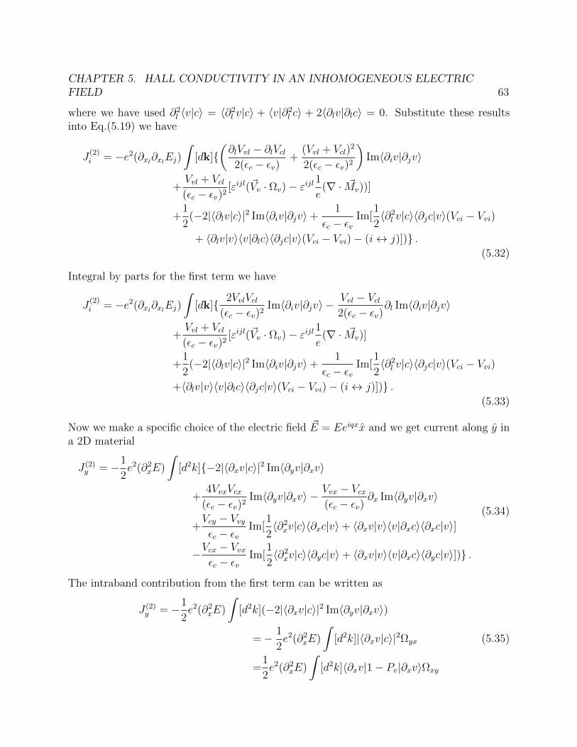
CHAPTER 5. HALL CONDUCTIVITY IN AN INHOMOGENEOUS ELECTRICFIELD 63
where we have used ∂2l 〈v|c〉 = 〈∂2
l v|c〉 + 〈v|∂2l c〉 + 2〈∂lv|∂lc〉 = 0. Substitute these results
into Eq.(5.19) we have
J(2)i = −e2(∂xl∂xlEj)
∫[dk]
(∂lVvl − ∂lVcl
2(εc − εv)+
(Vvl + Vcl)2
2(εc − εv)2
)Im〈∂iv|∂jv〉
+Vvl + Vcl(εc − εv)2
[εijl(~Vv · Ωv)− εijl1
e(∇ · ~Mv))]
+1
2(−2|〈∂lv|c〉|2 Im〈∂iv|∂jv〉+
1
εc − εvIm[
1
2〈∂2l v|c〉〈∂jc|v〉(Vci − Vvi)
+ 〈∂lv|v〉〈v|∂lc〉〈∂jc|v〉(Vci − Vvi)− (i↔ j)]) .(5.32)
Integral by parts for the first term we have
J(2)i = −e2(∂xl∂xlEj)
∫[dk] 2VvlVcl
(εc − εv)2Im〈∂iv|∂jv〉 −
Vvl − Vcl2(εc − εv)
∂l Im〈∂iv|∂jv〉
+Vvl + Vcl(εc − εv)2
[εijl(~Vv · Ωv)− εijl1
e(∇ · ~Mv)]
+1
2(−2|〈∂lv|c〉|2 Im〈∂iv|∂jv〉+
1
εc − εvIm[
1
2〈∂2l v|c〉〈∂jc|v〉(Vci − Vvi)
+〈∂lv|v〉〈v|∂lc〉〈∂jc|v〉(Vci − Vvi)− (i↔ j)]) .(5.33)
Now we make a specific choice of the electric field ~E = Eeiqxx and we get current along y ina 2D material
J (2)y = −1
2e2(∂2
xE)
∫[d2k]−2|〈∂xv|c〉|2 Im〈∂yv|∂xv〉
+4VvxVcx
(εc − εv)2Im〈∂yv|∂xv〉 −
Vvx − Vcx(εc − εv)
∂x Im〈∂yv|∂xv〉
+Vcy − Vvyεc − εv
Im[1
2〈∂2xv|c〉〈∂xc|v〉+ 〈∂xv|v〉〈v|∂xc〉〈∂xc|v〉]
−Vcx − Vvxεc − εv
Im[1
2〈∂2xv|c〉〈∂yc|v〉+ 〈∂xv|v〉〈v|∂xc〉〈∂yc|v〉]) .
(5.34)
The intraband contribution from the first term can be written as
J (2)y = −1
2e2(∂2
xE)
∫[d2k](−2|〈∂xv|c〉|2 Im〈∂yv|∂xv〉)
=− 1
2e2(∂2
xE)
∫[d2k]|〈∂xv|c〉|2Ωyx
=1
2e2(∂2
xE)
∫[d2k]〈∂xv|1− Pv|∂xv〉Ωxy
(5.35)
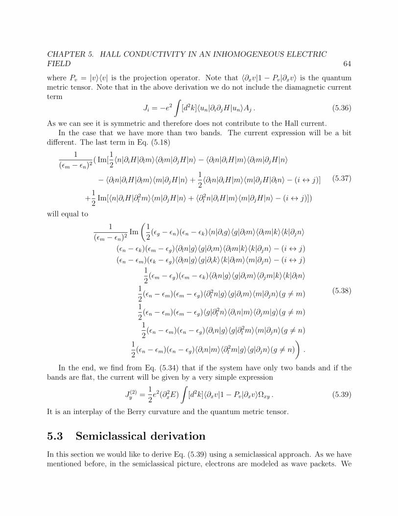
CHAPTER 5. HALL CONDUCTIVITY IN AN INHOMOGENEOUS ELECTRICFIELD 64
where Pv = |v〉〈v| is the projection operator. Note that 〈∂xv|1 − Pv|∂xv〉 is the quantummetric tensor. Note that in the above derivation we do not include the diamagnetic currentterm
Ji = −e2
∫[d2k]〈un|∂i∂jH|un〉Aj . (5.36)
As we can see it is symmetric and therefore does not contribute to the Hall current.In the case that we have more than two bands. The current expression will be a bit
different. The last term in Eq. (5.18)
1
(εm − εn)2( Im[
1
2〈n|∂iH|∂lm〉〈∂lm|∂jH|n〉 − 〈∂ln|∂iH|m〉〈∂lm|∂jH|n〉
− 〈∂ln|∂iH|∂lm〉〈m|∂jH|n〉+1
2〈∂ln|∂iH|m〉〈m|∂jH|∂ln〉 − (i↔ j)]
+1
2Im[〈n|∂iH|∂2
lm〉〈m|∂jH|n〉+ 〈∂2l n|∂iH|m〉〈m|∂jH|n〉 − (i↔ j)])
(5.37)
will equal to
1
(εm − εn)2Im
(1
2(εg − εn)(εn − εk)〈n|∂ig〉〈g|∂lm〉〈∂lm|k〉〈k|∂jn〉
(εn − εk)(εm − εg)〈∂ln|g〉〈g|∂im〉〈∂lm|k〉〈k|∂jn〉 − (i↔ j)
(εn − εm)(εk − εg)〈∂ln|g〉〈g|∂ik〉〈k|∂lm〉〈m|∂jn〉 − (i↔ j)
1
2(εm − εg)(εm − εk)〈∂ln|g〉〈g|∂im〉〈∂jm|k〉〈k|∂ln〉
1
2(εn − εm)(εm − εg)〈∂2
l n|g〉〈g|∂im〉〈m|∂jn〉(g 6= m)
1
2(εn − εm)(εm − εg)〈g|∂2
l n〉〈∂in|m〉〈∂jm|g〉(g 6= m)
1
2(εn − εm)(εn − εg)〈∂in|g〉〈g|∂2
lm〉〈m|∂jn〉(g 6= n)
1
2(εn − εm)(εn − εg)〈∂in|m〉〈∂2
lm|g〉〈g|∂jn〉(g 6= n)
).
(5.38)
In the end, we find from Eq. (5.34) that if the system have only two bands and if thebands are flat, the current will be given by a very simple expression
J (2)y =
1
2e2(∂2
xE)
∫[d2k]〈∂xv|1− Pv|∂xv〉Ωxy . (5.39)
It is an interplay of the Berry curvature and the quantum metric tensor.
5.3 Semiclassical derivation
In this section we would like to derive Eq. (5.39) using a semiclassical approach. As we havementioned before, in the semiclassical picture, electrons are modeled as wave packets. We
CHAPTER 5. HALL CONDUCTIVITY IN AN INHOMOGENEOUS ELECTRICFIELD 65
construct a wavepacket centered at xc and kc with the eigenstates within a single band.
|Ψ〉 =
∫[d2k] a(~k, t)ψ~k(x, t) (5.40)
~xc = 〈Ψ|x|Ψ〉 (5.41)
~kc =
∫[d2k]~k|a(~k, t)|2. (5.42)
In a static inhomogeneous electric field ~E = xEeiqx = −∇φ(x)the local Hamiltonian thatsuch a wave packet feels will be
H = H0(~k)− e[φ(xc) +
dφ
dx
∣∣∣∣xc
〈Ψ|(x− xc)|Ψ〉+1
2
d2φ
dx2
∣∣∣∣xc
〈Ψ|(x− xc)2|Ψ〉]
+ · · ·
= H0(~k)− e(φ(xc)−
1
2
dE
dx
∣∣∣∣xc
〈Ψ|(x− xc)2|Ψ〉+ · · ·).
(5.43)
We have used the fact that the wave packet is centered at xc. Since the wavepacket is not apoint particle, in the expansion above we have extra terms other than the electrical potential−eφ(xc). We work on the first non-zero term
〈Ψ|(x− xc)2|Ψ〉 = 〈Ψ|x2|Ψ〉 − x2c
=
∫[d2k]
∫[d2k′]a ∗ (k, t)a(k′, t) 〈ψnk|x2|ψnk′〉 − x2
c
=∑m
∫[d2k′′]
∫[d2k]
∫[d2k′]a ∗ (k, t)a(k′, t) 〈ψnk|x|ψmk′′〉 〈ψmk′′ |x|ψnk′〉 − x2
c .
(5.44)
If m 6= n it will be∑m
∫[d2k′′]
∫[d2k]
∫[d2k′]a ∗ (k, t)a(k′, t)δ(k′′ − k′)δ(k − k′′)〈unk|i
∂umk∂kx〉〈umk|i
∂unk∂kx〉
=
∫[d2k]|a(k, t)|2
⟨∂unk∂kx
∣∣∣∣1− Pn∣∣∣∣∂unk∂kx
⟩=
⟨∂unk∂kx
∣∣∣∣1− Pn∣∣∣∣∂unk∂kx
⟩∣∣∣∣k=kc
.
(5.45)
If n = m it will be∫[d2k′′]
∫[d2k]
∫[d2k′]a∗(k, t)a(k′, t)
[(i∂
∂kx+ 〈unk|i
∂unk∂kx〉)δ(k − k′′)
]·[(−i ∂∂k′x
+ 〈unk′ |i∂unk′
∂k′x〉)δ(k′ − k′′)
]=
∫[d2k]
[(−i ∂∂kx
+ 〈unk|i∂unk∂kx〉)a∗(k, t)
] [(i∂
∂kx+ 〈unk|i
∂unk∂kx〉)a(k, t)
].
(5.46)

CHAPTER 5. HALL CONDUCTIVITY IN AN INHOMOGENEOUS ELECTRICFIELD 66
Writing the amplitude a(k, t) in the form of |a(k, t)|e−iγ(q,t) Eq.(5.46) will be∫[d2k]
[−ieiγ ∂|a(k, t)|
∂kx+ a∗(k, t)
∂γ
∂kx+ 〈unk|i
∂unk∂kx〉a∗(k, t)
]·[ie−iγ
∂|a(k, t)|∂kx
+ a(k, t)∂γ
∂kx+ 〈unk|i
∂unk∂kx〉a(k, t)
]= x2
c +
∫[d2k]
(∂|a|∂kx
)2
(5.47)
where we have used
xc =∂γ(kc, t)
∂kcx+ 〈unk|i
∂unk∂kcx
〉 . (5.48)
Finally we have
〈Ψ|(x− xc)2|Ψ〉 =
⟨∂un∂kx
∣∣∣∣1− Pn∣∣∣∣∂un∂kx
⟩∣∣∣∣~k= ~kc
+
∫[d2k]
(∂|a|∂kx
)2
(5.49)
The first term is the quantum metric tensor, which describes the intrinsic contribution fromthe Bloch waves while the second term is related to the details of how the wave packetis constructed. Due to the first term in Eq. (5.49) we will have a correction term to thesemiclassical equation for the response to an inhomogeneous electric field. The semiclassicalequation will be modified by
~kc = −e(E(xc) +
1
2
d2E(xc)
dx2c
⟨∂un∂kcx
∣∣∣∣1− Pn∣∣∣∣ ∂un∂kcx
⟩)x . (5.50)
The Hall velocity we will get from the second term is
δ~xc = −δ~kc × ~Ω = e1
2
d2E(xc)
dx2c
⟨∂un∂kcx
∣∣∣∣1− Pn∣∣∣∣ ∂un∂kcx
⟩Ωxyy (5.51)
which leads to the Hall current
δJy = e2 1
2
d2E
dx2
∫[d2k]
⟨∂un∂kx
∣∣∣∣1− Pn∣∣∣∣∂un∂kx
⟩Ωxy . (5.52)
The result is the same as Eq. (5.39).There are two comments for the quantum metric tensor and the semiclassical approach:
1. In the Fourier transform we have the relation 4x ·4k ≥ 12. If we make our wavepacket
more localized in real space, the width of it in k space will be larger. However, theintrinsic contribution to the Hall conductivity from the Bloch waves unk is independentof how one construct the wave packet.
2. The quantum metric tensor also appears in construction of the maximally localizedWannier functions [50]. It is the gauge invariant part of the maximally localized Wan-nier function. For Chern insulators the Wannier function can not be localized in bothdirections of the two dimensional space. However, we can still have a well definedlocalization length in one direction.

CHAPTER 5. HALL CONDUCTIVITY IN AN INHOMOGENEOUS ELECTRICFIELD 67
5.4 Numerical results for Chern insulators
5.4.1 Topological flat band model
First, we study the Hall conductivity in a topological flat band model. There have been sev-eral papers studying how to construct 2D lattice tight binding models to produce topologicalflat bands. Their purpose is to study whether the analytic structure of the wave functionsassociated with the 2D Landau level is necessary for the fractional quantum Hall state. Herewe choose one of the proposed models. It is a two band Chern insulator with two nearlyflat bands. The details of this model can be found in [81]. Basically it is modified Haldanemodel [31] with fine tuned parameters.
We compute the Hall conductivity in the zeroth order and the second order in q. TheHall conductivity in the zeroth order is −3 with e = 1, h = 1. For computing the hallconductivity in the second order in q we use two ways. One is that we use our Eq. (5.39)which is valid for a two band insulator when the bands are flat,
J (2)y =
1
2e2(∂2
xE)
∫[d2k]〈∂xv|1− Pv|∂xv〉Ωxy . (5.53)
This would not be the correct result since there are other terms contributing to the hallconductivity when the bands are not entirely flat. However, it should be very close to theright value since the model we choose has two nearly flat bands. To get the right value wecompute it using the expression from Kubo formula which includes all contributions. Indeed,we get the value 0.44 from Eq. (5.39) and 0.43 from the expression including all contributionswith e = 1, h = 1 and they are very close to each other.
5.4.2 Hofstadter model
In the Hofstadter model, each plaquette in a two dimensional lattice encloses a magneticflux φ = φ0
nwhere φ0 is one magnetic flux quantum h
2e. The Hofstadter model will converge
to continuum Landau levels in the small flux limit n → ∞. Therefore, in the small fluxlimit we expect to have C2 = −3
4with the filling factor ν = 1. In this section, we get the
numerical results of C2 for each value of n in a Hofstadter model. In the following we willalways work with ν = 1 and we set e = 1, ~ = 1, and the area of each plaquette as 1.
As we can see from Fig.5.1, C2 is approaching to a constant as n grows. We do linearfitting for C2 in Fig.5.2 and the linear fitting function is approximately
C2 = −3
4+
2π
8n(5.54)
The constant term is −34
as expected.As we have discussed before, C2 can be divided into two parts, one is related to the Hall
viscosity and the other is related to the magnetic susceptibility
C2 =ηA
~n− 2π
ν
`2
~ωcB2ε′′(B) . (5.55)

CHAPTER 5. HALL CONDUCTIVITY IN AN INHOMOGENEOUS ELECTRICFIELD 68
0 100 200 300 400n
0.75
0.74
0.73
0.72
0.71
0.70
0.69
0.68C 2
Figure 5.1: The coefficient C2 of the q2 term in Hall conductivity for a Hofstadter modelwith 1
nflux quantum in each plaquette.
0.0025 0.0030 0.0035 0.0040 0.00451n
0.74800
0.74775
0.74750
0.74725
0.74700
0.74675
0.74650
0.74625
C 2
C2 = 0.750 + 0.787/n
Figure 5.2: Linear fitting for the coefficient C2 of the q2 term in Hall conductivity for aHofstadter model with 1
nflux quantum in each plaquette.

CHAPTER 5. HALL CONDUCTIVITY IN AN INHOMOGENEOUS ELECTRICFIELD 69
0.0250 0.0275 0.0300 0.0325 0.0350 0.0375 0.0400 0.0425B (2
n )
3.9750
3.9725
3.9700
3.9675
3.9650
3.9625
3.9600
3.9575
ene
rgy
energy = -4.00 + 0.99 * B
Figure 5.3: The electron energy per unit cell vs the magnetic field B.
If we can get the value of ε′′(B) we will have the value of Hall viscosity ηA. There are twoways we can compute ε′′(B). One is that we can get it from the electron energy which is afunction of the magnetic field. We plot the relation between the one electron energy per unitcell and the magnetic field for the Hofstadter model and do linear fitting. From the fittingresult in Fig.5.4.2 we see that the one electron energy per unit cell is linear in the magneticfield in the small flux limit. We thus have
ε(B) · 2π`2B = ε(B) · 2π
B= B + const (5.56)
and the magnetic susceptibility will be
ε′′(B) =2
2π. (5.57)
As we know, the magnetic susceptibility of the quantum Hall state at ν = 1 is
ε′′(B) =1
2πm. (5.58)
By comparing with Eq. (5.57) we can get the mass m = 12. It is because in the small flux
limit the energy dispersion is k2 near k = 0 .Another way to compute the magnetic susceptibility is from the symmetric part of the
conductivity tensor in the second order in q. The conductivity tensor can be divided intotwo parts according to Read’s paper [15]
σij(q, w) =1
m2w2c
[iκ−1
w+qµqνεµiενj + (ηH(w = 0)− κ−1
wc)q2εij] (5.59)

CHAPTER 5. HALL CONDUCTIVITY IN AN INHOMOGENEOUS ELECTRICFIELD 70
0 50 100 150 200 250 300 350n
1.5
1.6
1.7
1.8
1.9
2.0
′′ (B)*
2
Figure 5.4: Magnetic susceptibility of a Hofstadter model with 1n
flux quantum in eachplaquette of the 2d lattice.
whereκ−1(ν,B) = B2ε′′(B) . (5.60)
The first term is symmetric in i ↔ j and the second term is the hall conductivity tensor.Therefore, we can compute the symmetric part of the conductivity tensor to get the magneticsusceptibility using the Kubo formula
σSij = − e2
iw
∫[dk]
∑n,m
f(εn,k−qx/2)− f(εm,k+qx/2)
εn,k−qx/2 − εm,k+qx/2
(5.61)
· Re[〈nk−qx/2|∂iH|mk+qx/2〉〈mk+qx/2|∂jH|nk−qx/2〉] . (5.62)
We plot the values and do linear fitting in Fig.5.5. The fitting function is approximately
ε′′(B) =2
2π− 3
4n. (5.63)
We reach the same conclusion that ε′′(B) = 22π
and with that we have ηA = 14
as expected.

CHAPTER 5. HALL CONDUCTIVITY IN AN INHOMOGENEOUS ELECTRICFIELD 71
0.0028 0.0030 0.0032 0.0034 0.00361n
1.983
1.984
1.985
1.986
1.987
′′ (B)*
2
′′(B) * 2 = 2.000 4.696/n
Figure 5.5: Linear fitting for the magnetic susceptibility of a Hofstadter model with 1n
fluxquantum in each plaquette of the 2d lattice.

72
Bibliography
[1] S. Adler. In: Phys. Rev. 177 (1969), p. 2426.
[2] V. M. Agranovich and V. L. Ginzburg. Crystal Optics with Spatial Dispersion, andExcitons. 2nd. Berlin: Springer, 1984.
[3] V. M. Agranovich and V. I. Yudson. In: Opt. Commun. 9 (1973), p. 58.
[4] P. B. Allen. “Electron Transport”. In: Conceptual foundations of materials properties:A standard model for calculation of ground- and excited-state properties. Ed. by S. G.Louie and M. L. Cohen. Vol. 1. Contemporary Concepts of Condens. Matt. Science.Elsevier, 2006, p. 165.
[5] N. P. Armitage. “Constraints on Jones transmission matrices from time-reversal in-variance and discrete spatial symmetries”. In: Phys. Rev. B 90 (2014), p. 035135.
[6] N. W. Ashcroft and N. D. Mermin. Solid State Physics. Brooks Cole, 1976.
[7] N.W. Ashcroft and N.D. Mermin. Solid State Physics. Philadelphia: Saunders College,1976.
[8] J. E. Avron, R. Seiler, and P. G. Zograf. “Viscosity of Quantum Hall Fluids”. In: Phys.Rev. Lett. 75 (1995), pp. 697–700.
[9] L. Barron. Molecular Light Scattering and Optical Activity. Cambridge: CambridgeUniversity Press, 2004.
[10] J. S. Bell and R. Jackiw. In: Nuovo Cimento 60A (1969), p. 4.
[11] M. V. Berry. “Quantal phase factors accompanying adiabatic changes”. In: Proc. R.Soc. London, Ser. A 392 (1984), p. 1802.
[12] M. V. Berry. “The quantum phase, five years after”. In: Geometric Phases in Physics(1989).
[13] E. I. Blount. In: Solid State Physics 13 (1962), p. 305.
[14] V. V Bokut and A .N Serkyukov. In: Prikl. Spectrosk. 20 (1974), p. 677.
[15] Barry Bradlyn, Moshe Goldstein, and N. Read. “Kubo formulas for viscosity: Hallviscosity, Ward identities, and the relation with conductivity”. In: Phys. Rev. B 86 (242012), p. 245309.
[16] A. D. Buckingham and M. D. Dunn. In: J. Chem. Soc. A (1971), p. 1988.

BIBLIOGRAPHY 73
[17] M.-C. Chang and M.-F.Yang. In: Phys. Rev. B 91 (2015), p. 115203.
[18] M.-C. Chang and M.-F. Yang. In: Phys. Rev. B 92 (2015), p. 205201.
[19] Y. Chen, S. Wu, and A. A. Burkov. In: Phys. Rev. B 88 (2013), p. 125105.
[20] H Diehl et al. “Spin photocurrents in (110)-grown quantum well structures”. In: NewJ. Phys. 9.9 (2007), p. 349.
[21] M. Dressel and G. Gruner. Electrodynamics of Solids. Cambridge, 2002.
[22] Andrew M. Essin et al. “Orbital magnetoelectric coupling in band insulators”. In:Phys. Rev. B 81 (20 2010), p. 205104.
[23] H. D. Flack. In: Helv. Chim. Acta 86 (2003), p. 905.
[24] Alexander D. Fried. “Relationship of time-reversal symmetry breaking to optical Kerrrotation”. In: Phys. Rev. B 90 (2014), p. 121112.
[25] S. D. Ganichev et al. “Conversion of Spin into Directed Electric Current in QuantumWells”. In: Phys. Rev. Lett. 86 (19 2001), pp. 4358–4361.
[26] Y. Gao, S. A. Yang, and Q. Niu. In: Phys. Rev. B 91 (2015), p. 214405.
[27] D. Gosalbez-Martınez, I. Souza, and D. Vanderbilt. In: Phys. Rev. B 92 (2015), p. 085138.
[28] P. Goswami, G. Sharma, and S. Tewari. In: Phys. Rev. B 92 (2015), 161110(R).
[29] P. Goswami and S. Tewari. In: arXiv:1311.1506 (2013).
[30] F. D. M. Haldane. In: Phys. Rev. Lett. 93 (2004), p. 206602.
[31] F. D. M. Haldane. “Model for a Quantum Hall Effect without Landau Levels: Condensed-Matter Realization of the ”Parity Anomaly””. In: Phys. Rev. Lett. 61 (18 1988),pp. 2015–2018.
[32] B Halperin. “The Hunt for Anyon Superconductivity”. In: The Physics and Chemistryof Oxide Superconductors. Ed. by Y. Iye and H. Yasuoka. Springer Verlag Proceedingsof Physics Vol 60. Springer-Verlag, Berlin, 1992, p. 439.
[33] W. A. Harrison. Solid State Theory. New York: Dover, 1980.
[34] R. M. Hornreich and S. Shtrikman. In: Phys. Rev. 171 (1968), p. 1065.
[35] Pavan Hosur and Xiao-Liang Qi. In: Phys. Rev. B 91 (2015), p. 081106.
[36] P. Hosur et al. In: Phys. Rev. B 87 (2013), p. 115116.
[37] Carlos Hoyos and Dam Thanh Son. “Hall Viscosity and Electromagnetic Response”.In: Phys. Rev. Lett. 108 (6 2012), p. 066805.
[38] S.-M. Huang et al. In: arXiv:1503.05868 (2015).
[39] Xiaochun Huang et al. “Observation of the Chiral-Anomaly-Induced Negative Magne-toresistance in 3D Weyl Semimetal TaAs”. In: Phys. Rev. X 5 (3 2015), p. 031023.
[40] Zhou Jian-Hui et al. “Topological Invariants of Metals and the Related Physical Ef-fects”. In: Chinese Physics Letters 30.2 (2013), p. 027101.

BIBLIOGRAPHY 74
[41] D. E. Kharzeev. In: Prog. Part. Nucl. Phys. 75 (2014), p. 133.
[42] R. D. King-Smith and David Vanderbilt. “Theory of polarization of crystalline solids”.In: Phys. Rev. B 47 (3 1993), pp. 1651–1654.
[43] Sigmund Kohler, Jorg Lehmann, and Peter Hanggi. “Driven quantum transport on thenanoscale”. In: Physics Reports 406.6 (2005), pp. 379–443.
[44] L. D. Landau and E. M. Lifshitz. Electrodynamics of Continuous Media. 2nd. Oxford:Pergamon Press, 1984.
[45] L. D. Landau and E. M. Lifshitz. Theory of Elasticity. Oxford: Pergamon Press, 1986.
[46] Tian Liang et al. “Ultrahigh mobility and giant magnetoresistance in the Dirac semi-metal Cd3As2”. In: Nature Materials 14.3 (2014), pp. 280–284.
[47] J. Ma and D. A. Pesin. In: Phys. Rev. B 92 (2015), p. 235205.
[48] A. Malashevich and I. Souza. In: Phys. Rev. B 82 (2010), p. 245118.
[49] Andrei Malashevich et al. “Theory of orbital magnetoelectric response”. In: New Jour-nal of Physics 12.5 (2010), p. 053032.
[50] Nicola Marzari and David Vanderbilt. “Maximally localized generalized Wannier func-tions for composite energy bands”. In: Phys. Rev. B 56 (20 1997), pp. 12847–12865.
[51] D. B. Melrose and R. C. McPhedran. Electromagnetic Processes in Dispersive Media.Cambridge: Cambridge University Press, 1991.
[52] Takahiro Morimoto and Naoto Nagaosa. “Topological nature of nonlinear optical effectsin solids”. In: 2.5 (2016), e1501524.
[53] Naoto Nagaosa et al. “Anomalous Hall effect”. In: Rev. Mod. Phys. 82 (2 2010),pp. 1539–1592.
[54] K. Natori. In: J. Phys. Soc. Japan 39 (1975), p. 1013.
[55] R. E. Newnham. Properties of Materials. Oxford: Oxford University Press, 2005.
[56] H. B. Nielsen and M. Ninomiya. In: Phys. Lett. 130B (1983), p. 389.
[57] H. Nielsen and M. Ninomiya. In: Nucl. Phys. B185 (1981), p. 20.
[58] H.B. Nielsen and M Ninomiya. “Berry phase mechanism for optical gyrotropy in stripe-ordered cuprates”. In: Nucl. Phys. B 185 (16 1981), p. 20.
[59] Takashi Oka and Hideo Aoki. “Photovoltaic Hall effect in graphene”. In: Phys. Rev. B79 (8 2009), p. 081406.
[60] P. Olbrich et al. “Observation of the orbital circular photogalvanic effect”. In: Phys.Rev. B 79 (12 2009), p. 121302.
[61] J. Orenstein and Joel E. Moore. In: Phys. Rev. B 87 (2013), p. 165110.
[62] Francesco M. D. Pellegrino, Mikhail I. Katsnelson, and Marco Polini. “Helicons in Weylsemimetals”. In: Phys. Rev. B 92 (20 2015), p. 201407.

BIBLIOGRAPHY 75
[63] Xiao-Liang Qi, Taylor L. Hughes, and Shou-Cheng Zhang. “Topological field theory oftime-reversal invariant insulators”. In: Phys. Rev. B 78 (19 2008), p. 195424.
[64] Inti Sodemann and Liang Fu. “Quantum Nonlinear Hall Effect Induced by Berry Cur-vature Dipole in Time-Reversal Invariant Materials”. In: Phys. Rev. Lett. 115 (21 2015),p. 216806.
[65] D. T. Son and B. Z. Spivak. In: Phys. Rev. B 88 (2013), p. 104412.
[66] D. T. Son and N. Yamamoto. In: Phys. Rev. Lett. 109 (2012), p. 181602.
[67] Ganesh Sundaram and Qian Niu. “Wave-packet dynamics in slowly perturbed crys-tals: Gradient corrections and Berry-phase effects”. In: Phys. Rev. B 59 (23 1999),pp. 14915–14925.
[68] D. J. Thouless. “Quantization of particle transport”. In: Phys. Rev. B 27 (10 1983),pp. 6083–6087.
[69] D. J. Thouless et al. In: Phys. Rev. Lett. 49 (1982), p. 405.
[70] Daniel Varjas et al. “Dynamical Piezoelectric and Magnetopiezoelectric Effects in PolarMetals from Berry Phases and Orbital Moments”. In: Phys. Rev. Lett. 117 (25 2016),p. 257601.
[71] M. M. Vazifeh and M. Franz. In: Phys. Rev. Lett. 111 (2013), p. 027201.
[72] A .P. Vinogradov. In: Phys. Usp. 45 (2002), p. 331.
[73] Hongming Weng et al. “Weyl Semimetal Phase in Noncentrosymmetric Transition-Metal Monophosphides”. In: Phys. Rev. X 5 (1 2015), p. 011029.
[74] F. Wooten. Optical Properties of Solids. New York: Academic Press, 1972.
[75] D. Xiao, M.-C. Chang, and Q. Niu. In: Rev. Mod. Phys. 82 (2010), p. 1959.
[76] Di Xiao, Ming-Che Chang, and Qian Niu. “Berry phase effects on electronic proper-ties”. In: Rev. Mod. Phys. 82 (3 2010), pp. 1959–2007.
[77] Di Xiao, Junren Shi, and Qian Niu. “Berry Phase Correction to Electron Density ofStates in Solids”. In: Phys. Rev. Lett. 95 (13 2005), p. 137204.
[78] J. Xiong et al. “Evidence for the chiral anomaly in the Dirac semimetal Na3Bi”. In:Science 350.6259 (2015), pp. 413–416.
[79] Y. Yafet. In: Solid State Physics 14 (1963), p. 1.
[80] N. Yamamoto. In: Phys. Rev. D 92 (2015), p. 085011.
[81] Shuo Yang et al. “Topological flat band models with arbitrary Chern numbers”. In:Phys. Rev. B 86 (24 2012), p. 241112.
[82] W. Yao, D. Xiao, and Q. Niu. In: Phys. Rev. B 77 (2008), p. 235406.
[83] T. Yoda, T. Yokoyama, and S. Murakami. In: Sci. Rep. 5 (2015), p. 12024.
[84] S. M. Young et al. In: Phys. Rev. Lett. 108 (2012), p. 140405.
BIBLIOGRAPHY 76
[85] Shudan Zhong, Joel E. Moore, and Ivo Souza. “Gyrotropic Magnetic Effect and theMagnetic Moment on the Fermi Surface”. In: Phys. Rev. Lett. 116 (7 2016), p. 077201.
[86] Shudan Zhong, Joseph Orenstein, and Joel E. Moore. In: Phys. Rev. Lett. 115 (2015),p. 117403.
[87] J.-H. Zhou et al. In: Chin. Phys. Lett. 30 (2013), p. 027101.
[88] A. A. Zyuzin, S. Wu, and A. A. Burkov. In: Phys. Rev. B 85 (2012), p. 165110.


![6. СОВЕТУВАЊЕ · [3] M. R. Popnikolova, M. Cundev, L.Petkovska, “Nonlinear Electromagnetic Field Calculation in Solid Salient Poles synchronous Motor”, Proc. Of EPNC](https://static.fdocuments.in/doc/165x107/5f2cf8f969a71e25b05d3706/6-3-m-r-popnikolova-m-cundev-lpetkovska-aoenonlinear.jpg)

![Nonlinear Electroelastic Deformations · the theoretical foundations of electromagnetic continua within a flnite defor- ... and Kovetz [10] and references ... as in elasticity theory,](https://static.fdocuments.in/doc/165x107/5b92154209d3f274268d3c01/nonlinear-electroelastic-deformations-the-theoretical-foundations-of-electromagnetic.jpg)


