Linear Algebraic Primitives for Parallel Computing on Large Graphs
301
UNIVERSITY OF CALIFORNIA Santa Barbara Linear Algebraic Primitives for Parallel Computing on Large Graphs A Dissertation submitted in partial satisfaction of the requirements for the degree of Doctor of Philosophy in Computer Science by Aydın Bulu¸ c Committee in Charge: Professor John R. Gilbert, Chair Professor Shivkumar Chandrasekaran Professor Frederic T. Chong Professor ¨ OmerN.E˘gecio˘glu March 2010
Transcript of Linear Algebraic Primitives for Parallel Computing on Large Graphs

UNIVERSITY OF CALIFORNIASanta Barbara
Linear Algebraic Primitives for Parallel
Computing on Large Graphs
A Dissertation submitted in partial satisfactionof the requirements for the degree of
Doctor of Philosophy
in
Computer Science
by
Aydın Buluc
Committee in Charge:
Professor John R. Gilbert, Chair
Professor Shivkumar Chandrasekaran
Professor Frederic T. Chong
Professor Omer N. Egecioglu
March 2010
The Dissertation ofAydın Buluc is approved:
Professor Shivkumar Chandrasekaran
Professor Frederic T. Chong
Professor Omer N. Egecioglu
Professor John R. Gilbert, Committee Chairperson
March 2010
Linear Algebraic Primitives for Parallel Computing on Large Graphs
Copyright© 2010
by
Aydın Buluc
iii

To my friend of misery.
iv
Acknowledgements
It is a great pleasure to thank everybody who made this thesis possible.
It is downright impossible to overstate how thankful I am to my advisor,
John R. Gilbert. He has been a magnificant advisor and a great role model in
all aspects: as a scientist, collaborator, teacher, and manager. He provided me
a great work environment, perfectly balanced between my thesis work and the
side projects that I wanted to pursue. This allowed me to enhance my breadth
of knowledge of the general areas of parallel computing, sparse linear algebra
and graph algorithms, without comprimising my depth of knowledge on my thesis
work. Especially during my junior years as his Ph.D. student, John was as patient
as a human being can ever be, pointing me to the right direction over and over
again, secretly knowing that I would keep on asking the same type of questions
for another three months until I would get mature enough to comprehend what
he had been trying to tell me from the very beginning. I will always remember
his amazing ability to motivate me without micromanaging.
I am grateful to all my committee members, for their time and valuable feed-
back. I am especially indebted to Omer N. Egecioglu for being my mentor from
the very first day I came to UCSB. He gave me more of his time than I probably
deserved. I want to thank Alan Edelman for officially hosting me during my visit
v
to MIT, and giving me the opportunity to meet extremely smart people from all
fields.
Special thanks to Charles E. Leiserson for his lead in reshaping our casual
research discussion into a real collaboration. I am truly amazed by his outstanding
scholarship and strong work ethics. The chapter on parallel sparse matrix-vector
multiplication is a reprint of the material resulted from that collaboration with
Jeremy T. Fineman and Matteo Frigo. I learned a lot from all three of them.
I am grateful to Erik Boman for having me at Sandia National Labs as a
summer intern in 2008. I thank all the folks in our group at Sandia/Albuquerque
for their company. Special thanks to Bruce Hendrickson for his support and
encouragement. As a great scientist, he has a unique ability to stay righteous
while speaking his opinions without reservations.
I would also like to thank my lab mates over the years: Viral Shah, Vikram
Aggarwal, Imran Patel, Stefan Karpinski and Adam Lugowski. Many times, our
conversations and meetings helped me think out of the box or sharpen my argu-
ments.
When it comes to who gets the most credits about who I become, my family can
simply not face competition. Thanks to “Annem ve Babam” who has supported
me and my decisions without reservations. I know they would make God their
enemy in this cause, if they had to.
vi
I would like to thank all my friends who made my journey enjoyable. Spe-
cial thanks to Murat Altay and Lutfiye Bulut for generously opening up their
apartment to me while I was visiting MIT. Many thanks to my off-county friends,
Simla Ceyhan and Osman Ertorer, for making North California my third home. I
am especially grateful to Ahmet Bulut, Petko Bogdanov, Ali Irturk, Arda Atalı,
Ceren Budak, Bahar Koymen, Emre Sargın, Basak Alper, Pegah Kamousi, Mike
Wittie and Lara Deek for their company at UCSB. Vlasia Anagnostopoulou gets
the most credit for reasons that will stay with me longer.
vii
Curriculum Vitæ
Aydın Buluc
Education
2009 Master of Science in Computer Science, UC Santa Barbara.
2005 Bachelor of Science in Computer Science, Sabanci University
Experience
2007 – Present Graduate Research Assistant, UC Santa Barbara.
2008 Summer Intern, Sandia National Labs
2006 Summer Intern, Citrix Online
2005 – 2007 Teaching Assistant, UC Santa Barbara.
Selected Publications
Aydın Buluc and John R. Gilbert. “On the Representation and Multiplication of Hyper-
sparse Matrices,” In Proceedings of the 22nd IEEE International Parallel and Distributed
Processing Symposium (IPDPS), April 2008.
Aydın Buluc and John R. Gilbert. “Challenges and Advances in Parallel Sparse Matrix-
Matrix Multiplication,” In Proceedings of the 37th International Conference on Parallel
Processing (ICPP), September, 2008.
Aydın Buluc , Jeremy T. Fineman, Matteo Frigo, John R. Gilbert, and Charles E. Leis-
erson “Parallel Sparse Matrix-Vector and Matrix-Transpose-Vector Multiplication using
viii
Compressed Sparse Blocks” In Proceedings of the 21st ACM Symposium on Parallelism
in Algorithms and Architectures (SPAA), August 2009.
Aydın Buluc , Ceren Budak, and John R. Gilbert. “Solving path problems on the GPU”,
Parallel Computing (2009), in press.
ix
Abstract
Linear Algebraic Primitives for Parallel Computing on
Large Graphs
Aydın Buluc
This dissertation presents a scalable high-performance software library to be
used for graph analysis and data mining. Large combinatorial graphs appear
in many applications of high-performance computing, including computational
biology, informatics, analytics, web search, dynamical systems, and sparse matrix
methods.
Graph computations are difficult to parallelize using traditional approaches
due to their irregular nature and low operational intensity. Many graph com-
putations, however, contain sufficient coarse grained parallelism for thousands of
processors that can be uncovered by using the right primitives. We will describe
the Parallel Combinatorial BLAS, which consists of a small but powerful set of
linear algebra primitives specifically targeting graph and data mining applications.
Given a set of sparse matrix primitives, our approach to developing a library
consists of three steps. We (1) design scalable parallel algorithms for the key
primitives, analyze their performance, and implement them on distributed mem-
ory machines, (2) develop reusable software and evaluate its performance, and
finally (3) perform pilot studies on emerging architectures.
x
The technical heart of this thesis is the development of a scalable sparse (gen-
eralized) matrix-matrix multiplication algorithm, which we use extensively as a
primitive operation for many graph algorithms such as betweenness centrality,
graph clustering, graph contraction, and subgraph extraction. We show that 2D
algorithms scale better than 1D algorithms for sparse matrix-matrix multiplica-
tion. Our 2D algorithms perform well in theory and in practice.
xi
Contents
Acknowledgements v
Curriculum Vitæ viii
Abstract x
List of Figures xvi
List of Tables xx
1 Introduction and Background 11.1 The Landscape of Parallel Computing . . . . . . . . . . . . . . . . 21.2 Parallel Graph Computations . . . . . . . . . . . . . . . . . . . . 61.3 The Case for Primitives . . . . . . . . . . . . . . . . . . . . . . . 11
1.3.1 A Short Survey of Primitives . . . . . . . . . . . . . . . . 121.3.2 Graph Primitives . . . . . . . . . . . . . . . . . . . . . . . 14
1.4 The Case for Sparse Matrices . . . . . . . . . . . . . . . . . . . . 151.5 Definitions and Conventions . . . . . . . . . . . . . . . . . . . . . 18
1.5.1 Synthetic R-MAT Graphs . . . . . . . . . . . . . . . . . . 191.5.2 Erdos-Renyi Random Graphs . . . . . . . . . . . . . . . . 191.5.3 Regular 3D Grids . . . . . . . . . . . . . . . . . . . . . . . 20
1.6 Contributions . . . . . . . . . . . . . . . . . . . . . . . . . . . . . 20
2 Implementing Sparse Matrices for Graph Algorithms 232.1 Introduction . . . . . . . . . . . . . . . . . . . . . . . . . . . . . . 232.2 Key Primitives . . . . . . . . . . . . . . . . . . . . . . . . . . . . 292.3 Triples . . . . . . . . . . . . . . . . . . . . . . . . . . . . . . . . . 32
2.3.1 Unordered Triples . . . . . . . . . . . . . . . . . . . . . . . 36
xii
2.3.2 Row-Ordered Triples . . . . . . . . . . . . . . . . . . . . . 422.3.3 Row-Major Ordered Triples . . . . . . . . . . . . . . . . . 50
2.4 Compressed Sparse Row/Column . . . . . . . . . . . . . . . . . . 552.4.1 CSR and Adjacency Lists . . . . . . . . . . . . . . . . . . 562.4.2 CSR on Key Primitives . . . . . . . . . . . . . . . . . . . . 58
2.5 Other Related Work and Conclusion . . . . . . . . . . . . . . . . 62
3 New Ideas in Sparse Matrix-Matrix Multiplication 643.1 Introduction . . . . . . . . . . . . . . . . . . . . . . . . . . . . . . 643.2 Sequential Sparse Matrix Multiply . . . . . . . . . . . . . . . . . . 69
3.2.1 Hypersparse Matrices . . . . . . . . . . . . . . . . . . . . . 733.2.2 Sparse Matrices with Large Dimension . . . . . . . . . . . 823.2.3 Performance of the Cache Efficient Algorithm . . . . . . . 88
3.3 Parallel Algorithms for Sparse GEMM . . . . . . . . . . . . . . . 903.3.1 1D Decomposition . . . . . . . . . . . . . . . . . . . . . . 903.3.2 2D Decomposition . . . . . . . . . . . . . . . . . . . . . . 913.3.3 Sparse 1D Algorithm . . . . . . . . . . . . . . . . . . . . . 913.3.4 Sparse Cannon . . . . . . . . . . . . . . . . . . . . . . . . 923.3.5 Sparse SUMMA . . . . . . . . . . . . . . . . . . . . . . . . 94
3.4 Analysis of Parallel Algorithms . . . . . . . . . . . . . . . . . . . 953.4.1 Scalability of the 1D Algorithm . . . . . . . . . . . . . . . 973.4.2 Scalability of the 2D Algorithms . . . . . . . . . . . . . . . 97
3.5 Performance Modeling of Parallel Algorithms . . . . . . . . . . . . 1003.5.1 Estimated Speedup of Parallel Algorithms . . . . . . . . . 1013.5.2 Scalability with Hypersparsity . . . . . . . . . . . . . . . . 105
3.6 Parallel Scaling of Sparse SUMMA . . . . . . . . . . . . . . . . . 1113.6.1 Experimental Design . . . . . . . . . . . . . . . . . . . . . 1113.6.2 Experimental Results . . . . . . . . . . . . . . . . . . . . . 113
3.7 Alternative Parallel Approaches . . . . . . . . . . . . . . . . . . . 1193.7.1 Load Balancing and Asynchronous Algorithms . . . . . . . 1193.7.2 Overlapping Communication with Computation . . . . . . 1243.7.3 Performance of the Asynchronous Implementation . . . . . 125
3.8 Future Work . . . . . . . . . . . . . . . . . . . . . . . . . . . . . . 130
4 The Combinatorial BLAS: Design and Implementation 1324.1 Motivation . . . . . . . . . . . . . . . . . . . . . . . . . . . . . . . 1324.2 Design Philosophy . . . . . . . . . . . . . . . . . . . . . . . . . . 133
4.2.1 The Overall Design . . . . . . . . . . . . . . . . . . . . . . 1334.2.2 The Combinatorial BLAS Routines . . . . . . . . . . . . . 135
4.3 A Reference Implementation . . . . . . . . . . . . . . . . . . . . . 141
xiii
4.3.1 The Software Architecture . . . . . . . . . . . . . . . . . . 1414.3.2 Management of Distributed Objects . . . . . . . . . . . . . 146
5 The Combinatorial BLAS: Applications and Performance Anal-ysis 1495.1 Betweenness Centrality . . . . . . . . . . . . . . . . . . . . . . . . 150
5.1.1 Parallel Strong Scaling . . . . . . . . . . . . . . . . . . . . 1535.1.2 Sensitivity to Batch Processing . . . . . . . . . . . . . . . 155
5.2 Markov Clustering . . . . . . . . . . . . . . . . . . . . . . . . . . 157
6 Parallel Sparse y ← Ax and y ← ATx Using Compressed SparseBlocks 1616.1 Introduction . . . . . . . . . . . . . . . . . . . . . . . . . . . . . . 1626.2 Conventional storage formats . . . . . . . . . . . . . . . . . . . . 1656.3 The CSB storage format . . . . . . . . . . . . . . . . . . . . . . . 1726.4 Matrix-vector multiplication using CSB . . . . . . . . . . . . . . . 1786.5 Analysis . . . . . . . . . . . . . . . . . . . . . . . . . . . . . . . . 1866.6 Experimental design . . . . . . . . . . . . . . . . . . . . . . . . . 1926.7 Experimental results . . . . . . . . . . . . . . . . . . . . . . . . . 2026.8 Conclusion . . . . . . . . . . . . . . . . . . . . . . . . . . . . . . . 211
7 Solving Path Problems on the GPU 2147.1 Introduction . . . . . . . . . . . . . . . . . . . . . . . . . . . . . . 2157.2 Algorithms Based on Block-Recursive Elimination . . . . . . . . . 218
7.2.1 The All-Pairs Shortest-Paths Problem . . . . . . . . . . . 2207.2.2 Recursive In-Place APSP Algorithm . . . . . . . . . . . . 223
7.3 GPU Computing Model with CUDA . . . . . . . . . . . . . . . . 2297.3.1 GPU Programming . . . . . . . . . . . . . . . . . . . . . . 2307.3.2 Experiences and Observations . . . . . . . . . . . . . . . . 232
7.4 Implementation and Experimentation . . . . . . . . . . . . . . . . 2357.4.1 Experimental Platforms . . . . . . . . . . . . . . . . . . . 2357.4.2 Implementation Details . . . . . . . . . . . . . . . . . . . . 2367.4.3 Performance Results . . . . . . . . . . . . . . . . . . . . . 2387.4.4 Comparison with Earlier Performance Results . . . . . . . 2417.4.5 Scalability and Resource Usage . . . . . . . . . . . . . . . 2447.4.6 Power and Economic Efficiency . . . . . . . . . . . . . . . 246
7.5 Conclusions and Future Work . . . . . . . . . . . . . . . . . . . . 249
8 Conclusions and Future Directions 251
xiv
Bibliography 256
Appendices 275
A Alternative One-Sided Communication Strategies for implement-ing Sparse GEMM 276
B Additional Timing Results on the APSP Problem 279
xv

List of Figures
2.1 A typical memory hierarchy . . . . . . . . . . . . . . . . . . . . . 272.2 Inner product formulation of matrix multiplication . . . . . . . . 302.3 Outer-product formulation of matrix multiplication . . . . . . . . 302.4 Row-wise formulation of matrix multiplication . . . . . . . . . . . 322.5 Column-wise formulation of matrix multiplication . . . . . . . . . 322.6 Multiply sparse matrices column-by-column . . . . . . . . . . . . 332.7 Matrix A (left) and an unordered triples representation (right) . 342.8 Operation y← Ax using triples . . . . . . . . . . . . . . . . . . 382.9 Scatters/Accumulates the nonzeros in the SPA . . . . . . . . . . 462.10 Gathers/Outputs the nonzeros in the SPA . . . . . . . . . . . . . 462.11 Operation C← A⊕B using row-ordered triples . . . . . . . . . 472.12 Operation C← AB using row-ordered triples . . . . . . . . . . . 492.13 Element-wise indexing of A(12, 16) on row-major ordered triples 512.14 Adjacency list (left) and CSR (right) representations of matrix Afrom Figure 2.7 . . . . . . . . . . . . . . . . . . . . . . . . . . . . . . 562.15 Operation y← Ax using CSR . . . . . . . . . . . . . . . . . . . 582.16 Operation C← AB using CSR . . . . . . . . . . . . . . . . . . . 61
3.1 Graph representation of the inner product A(i, :) ·B(:, j) . . . . 713.2 Graph representation of the outer product A(:, i) ·B(i, :) . . . . . 723.3 Graph representation of the sparse row times matrix product A(i, :) ·B . . . . . . . . . . . . . . . . . . . . . . . . . . . . . . . . . . . . . 723.4 2D Sparse Matrix Decomposition . . . . . . . . . . . . . . . . . . 743.5 Matrix A in CSC format . . . . . . . . . . . . . . . . . . . . . . . 753.6 Matrix A in Triples format . . . . . . . . . . . . . . . . . . . . . 763.7 Matrix A in DCSC format . . . . . . . . . . . . . . . . . . . . . 763.8 Nonzero structures of operands A and B . . . . . . . . . . . . . 783.9 Cartesian product and the multiway merging analogy . . . . . . . 79
xvi
3.10 Pseudocode for hypersparse matrix-matrix multiplication algorithm. . . . . . . . . . . . . . . . . . . . . . . . . . . . . . . . . . . . . . . . 813.11 Trends of different complexity measures for submatrix multiplica-tions as p increases . . . . . . . . . . . . . . . . . . . . . . . . . . . . . 833.12 Multiply sparse matrices column-by-column using a heap . . . . . 853.13 Subroutine to multiply bval with the next element from the ith listand insert it to the priority queue . . . . . . . . . . . . . . . . . . . . 863.14 Pseudocode for heap assisted column-by-column algorithm . . . . 873.15 Performance of two column-wise algorithms for multiplying twon× n sparse matrices from Erdos-Renyi random graphs . . . . . . . . 893.16 Operation C← AB using block row Sparse 1D algorithm . . . . 923.17 Circularly shift left by s along the processor row . . . . . . . . . . 933.18 Circularly shift up by s along the processor column . . . . . . . . 933.19 Operation C← AB using Sparse Cannon . . . . . . . . . . . . . 933.20 Sparse SUMMA Execution (b = n/
√p) . . . . . . . . . . . . . . . 94
3.21 Modeled speedup of Synchronous Sparse 1D algorithm . . . . . . 1023.22 Modeled speedup of synchronous Sparse Cannon . . . . . . . . . 1033.23 Modeled speedup of asynchronous Sparse Cannon . . . . . . . . . 1053.24 Model of scalability of SpGEMM kernels . . . . . . . . . . . . . . 1083.25 Observed speedup of of synchronous Sparse SUMMA . . . . . . . 1133.26 Fringe size per level during breadth-first search . . . . . . . . . . 1143.27 Weak scaling of R-MAT times a tall skinny Erdos-Renyi matrix . 1173.28 Strong scaling of multiplication with the restriction operator fromthe right . . . . . . . . . . . . . . . . . . . . . . . . . . . . . . . . . . . 1193.29 Load imbalance per stage for multiplying two RMAT matrices on256 processors using Sparse Cannon . . . . . . . . . . . . . . . . . . . 1223.30 Load imbalance during parallel multiplication of two RMAT matrices 1233.31 The split distribution of matrix A on a single processor row . . . 1253.32 Partial C++ code partial for asynchronous SpGEMM using one-sided communication and split prefetching for overlapping communica-tion with computation . . . . . . . . . . . . . . . . . . . . . . . . . . . 1263.33 Performances of the asynchronous and synchronous implementa-tions of the Sparse SUMMA . . . . . . . . . . . . . . . . . . . . . . . . 1273.34 Performance comparison of the asynchronous and synchronous im-plementations usign different number of cores per node . . . . . . . . . 128
4.1 Software architecture for matrix classes . . . . . . . . . . . . . . 1424.2 Partial C++ interface of the base SpMat class . . . . . . . . . . 1444.3 Distributed sparse matrix class and storage . . . . . . . . . . . . 147
xvii
5.1 Parallel strong scaling of the distributed-memory betweenness cen-trality implementation (smaller input sizes) . . . . . . . . . . . . . . . 1535.2 Parallel strong scaling of the distributed-memory betweenness cen-trality implementation (bigger input sizes) . . . . . . . . . . . . . . . . 1545.3 The effect of batch processing on the performance of the distributed-memory betweenness centrality implementation . . . . . . . . . . . . . 1565.4 Inflation code using the Combinatorial BLAS primitives . . . . . 1585.5 MCL code using the Combinatorial BLAS primitives . . . . . . . 1585.6 Strong scaling of the three most expensive iterations while cluster-ing an R-MAT graph of scale 14 using the MCL algorithm implementedusing the Combinatorial BLAS . . . . . . . . . . . . . . . . . . . . . . 160
6.1 Average performance of Ax and ATx operations on 13 differentmatrices from our benchmark test suite. . . . . . . . . . . . . . . . . . 1646.2 Parallel procedure for computing y ← Ax, where the n× n matrixA is stored in CSR format. . . . . . . . . . . . . . . . . . . . . . . . . 1676.3 Serial procedure for computing y ← ATx, where the n× n matrixA is stored in CSR format. . . . . . . . . . . . . . . . . . . . . . . . . 1706.4 Pseudocode for the matrix-vector multiplication y ← Ax. . . . . . 1806.5 Pseudocode for the subblockrow vector product y ← (AiℓAi,ℓ+1 · · ·Air)x. . . . . . . . . . . . . . . . . . . . . . . . . . . . . . . . . . . . . 1826.6 Pseudocode for the subblock-vector product y ←Mx. . . . . . . . 1856.7 The effect of block size parameter β on SpMV performance usingthe Kkt power matrix. . . . . . . . . . . . . . . . . . . . . . . . . . . . 1966.8 Structural information on the sparse matrices used in our experi-ments, ordered by increasing number of nonzeros. . . . . . . . . . . . 1996.9 CSB SpMV performance on Opteron (smaller matrices). . . . . 2036.10 CSB SpMV T performance on Opteron (smaller matrices). . . . 2046.11 CSB SpMV performance on Opteron (larger matrices). . . . . . 2056.12 CSB SpMV T performance on Opteron (larger matrices). . . . 2066.13 Average speedup results for relatively smaller (1–7) and larger (8–14) matrices. These experiments were conducted on Opteron. . . . . . 2066.14 Parallelism test for CSB SpMV on Asic 320k obtained by artifi-cially increasing the flops per byte . . . . . . . . . . . . . . . . . . . . 2076.15 CSB SpMV performance on Harpertown. . . . . . . . . . . . . . 2096.16 CSB SpMV performance on Nehalem. . . . . . . . . . . . . . . . 2106.17 Serial performance comparison of SpMV for CSB and CSR. . . . . 2116.18 Serial performance comparison of SpMV T for CSB and CSR. . . 2126.19 Performance comparison of parallel CSB SpMV with Star-P. . . 213
xviii
7.1 FW algorithm in the standard notation . . . . . . . . . . . . . . 2227.2 FW algorithm in linear algebra notation . . . . . . . . . . . . . . 2237.3 Pseudocode for recursive in-place APSP . . . . . . . . . . . . . . 2247.4 An example path in A∗
11 . . . . . . . . . . . . . . . . . . . . . . . 2267.5 Minimum-state DFA for the path expressions in A∗
11, starting stateis q0 . . . . . . . . . . . . . . . . . . . . . . . . . . . . . . . . . . . . . 2277.6 Stride-1 access per thread (row-major storage) . . . . . . . . . . 2347.7 A shapshot from the execution of the iterative algorithm . . . . . 2377.8 Log-log plot of absolute running times . . . . . . . . . . . . . . . 2417.9 Comparison of different GPU implementations on 8800 GTX settings 242
A.1 Strategy 1 . . . . . . . . . . . . . . . . . . . . . . . . . . . . . . . 278A.2 Strategy 2 . . . . . . . . . . . . . . . . . . . . . . . . . . . . . . . 278A.3 Strategies for matching the Post calls issued by multiple processors 278
xix

List of Tables
1.1 High-performance libraries and toolkits for parallel graph analysis 6
2.1 RAM Complexities of Key Primitives on Unordered and Row-Ordered Triples . . . . . . . . . . . . . . . . . . . . . . . . . . . . . . . 352.2 I/O Complexities of Key Primitives on Unordered and Row-OrderedTriples . . . . . . . . . . . . . . . . . . . . . . . . . . . . . . . . . . . . 362.3 RAM Complexities of Key Primitives on Row-Major Ordered Triplesand CSR . . . . . . . . . . . . . . . . . . . . . . . . . . . . . . . . . . 532.4 I/O Complexities of Key Primitives on Row-Major Ordered Triplesand CSR . . . . . . . . . . . . . . . . . . . . . . . . . . . . . . . . . . 54
4.1 Summary of the current API for the Combinatorial BLAS . . . . 139
7.1 GPU timings on GeForce 8800 Ultra (in milliseconds) . . . . . . . 2387.2 Speedup on 8800 Ultra w.r.t. the best CPU implementation . . . . 2397.3 Observed exponents and constants for the asymptotic behaviour ofour APSP implementations with increasing problem size . . . . . . . . 2407.4 Performance comparison of our best (optimized recursive) GPUimplementation with parallel Cilk++ code running on Neumann, usingall 16 cores . . . . . . . . . . . . . . . . . . . . . . . . . . . . . . . . . 2407.5 Comparisons of our best GPU implementation with the timingsreported for Han et al. ’s auto generation tool Spiral . . . . . . . . . . 2447.6 Scalability of our optimized recursive GPU implementation. Wetweaked core and memory clock rates using Coolbits. . . . . . . . . . . 2457.7 Scalability of our iterative GPU implementation. We tweaked coreand memory clock rates using Coolbits. . . . . . . . . . . . . . . . . . . 2457.8 Efficiency comparison of different architectures (running variouscodes), values in MFlops/Watts×sec (or equivalently MFlops/Joule) . 248
xx
B.1 Serial timings on Intel Core 2 Duo (in milliseconds) . . . . . . . . 279B.2 Serial timings on Opteron (in milliseconds) . . . . . . . . . . . . . 280
xxi
Chapter 1
Introduction and Background
Come, Come, Whoever You Are
Wonderer, worshipper, lover of leaving. It doesn’t matter.
Ours is not a caravan of despair.
Come, even if you have broken your vow a thousand times
Come, yet again, come, come.
Mevlana Celaleddin Rumi
This thesis provides a scalable high-performance software library, the Combi-
natorial BLAS, to be used for graph analysis and data mining. It targets parallel
computers and its main toolkit is composed of sparse linear algebraic operations.
In this chapter, I will try to give the motivation behind this work. Most
of these motivations are accompanied by historical background and references
to recent trends. The first section is a personal interpretation of the parallel
computing world as of early 2010. Section 1.2 reviews the state of the art of
parallel graph computations in practice. The following two sections, Sections 1.3
and 1.4, summarize the justifications of the two main ideas behind this thesis:
1

Chapter 1. Introduction and Background
the use of primitives and of sparse matrices. The final section summarizes the
contributions and provides an outline of this thesis.
1.1 The Landscape of Parallel Computing
It is no news that the economy is driving the past, present, and future of
computer systems. It was the economy that drove the “killer micro” [45] and
stalled innovative supercomputer design in the early 1990s. It is the economy that
is driving GPUs to get faster and forcing a unification of GPU/CPU architectures
today. It will be the economy that will drive energy efficient computing and
massive parallelism. This is partially due to a number of fundamental physical
limitations on sequential processing, such as the speed of light and the dissipation
of heat [156].
Although the literature contains several taxonomies of parallelism [85, 120,
176], one can talk about two fundamental types of parallelism available for ex-
ploitation in software: data parallelism and task parallelism. The former executes
the same instruction on a relatively large data set. For example, elementwise ad-
dition of two vectors has lots of data parallelism. Task parallelism, on the other
hand, is achieved by decomposing the application into multiple independent tasks
that can be executed as separate procedures. A multi-threaded web server pro-
2
Chapter 1. Introduction and Background
vides a good example for task parallelism, where multiple requests of different
kinds are handled in parallel. In reality, most applications use a combination of
data and task parallelism, and therefore, fall somewhere in the middle of the spec-
trum. Although it is possible to rewrite some applications that were previously
written in the data parallel fashion in a task parallel fashion, and vice versa, this
is not always possible.
In general, one can speak about a relationship between the current parallel
architectures and types of available parallelism. For example, massively multi-
threaded architectures [91, 129] are better than others when dealing with large
amounts of task parallelism. On the other side, GPUs [1, 2] excel in data parallel
computations. However, as most computations cannot be hard-classified as hav-
ing solely task parallelism or solely data parallelism, an ultimate direct mapping
of applications to architectures is unlikely to emerge.
From the late 1990s to the late 2000s, the supercomputing market was mostly
dominated by clusters made from commercial off-the-shelf processors. After this
decade of relative stability in parallel computing architectures, we are now expe-
riencing disruptions and divergences. Different application have different resource
requirements, leading to diversity and heterogeneity in parallel computing ar-
chitectures. On the other hand, the economic of scale dictate that a handful
general-purpose architectures that can be manufactured with low cost will domi-
3
Chapter 1. Introduction and Background
nate the HPC market. While building custom architectures that perfectly match
the underlying problem might be tempting for the HPC community, commodity
architectures have the advantage of achieving a much lower cost per unit. Special
purpose supercomputers, such as Anton [182], which is used to simulate molecular
dynamics of biological systems, will still find applications where the reward ex-
ceeds the cost. For broader range of applicability, however, supercomputers that
feature a balanced mixture of commodity and custom parts are likely to prevail.
Examples of currently available high-performance computing systems include
the following:
1. Distributed memory multiprocessors (such as the Cray XT4 and XT5) and
beowulf clusters that are primarily programmed using MPI. This class of
machines also include the RISC-based distributed-memory multi-processors
such as the IBM BlueGene [193],
2. ccNUMA and multicore architectures that are programmed either explicitly
through pthreads or through concurrency platforms like Cilk/Cilk++ [138],
OpenMP and Intel Building Blocks [167],
3. Massively multithreaded shared memory machines such as the Cray XMT [91]
and the Sun Niagara [129], and
4
Chapter 1. Introduction and Background
4. GPU or IBM Cell accelerated clusters. The largest scale example of the
latter (as of March 2010) is the Roadrunner system deployed at Los Alamos
National Laboratory [22].
Regardless of which architure(s) will prevail in the end, the economic trends
favor more parallelism in computing because building a parallel computer using
large number of simple processors has proved to be more efficient, both financially
and in terms of power, than using a small number of complex processors [181]. The
software world has to deal with this revolutionary change in computing. It is safe
to say that the software industry has been caught off-guard by this challenge. Most
programmers are not fundamentally trained to think “in parallel”. Many tools,
such as debuggers and profilers, that are taken for granted when writing sequential
programs, were (and still are) lacking for parallel software development. In the last
few years, there have been improvements towards making parallel programming
easier, including parallel debuggers [9, 199], concurrency platforms [138, 167], and
various domain specific libraries. Part of this thesis strives to be a significant
addition to the latter group of parallel libraries.
One of the most promising approaches for tackling the software challenge in
parallel computing is the top-down, application-driven, approach where common
algorithmic kernels in various important application domains are identified. In
the inspiring Berkeley Report [13], these kernels are called “dwarfs”(or “motifs”).
5

Chapter 1. Introduction and Background
This thesis is mostly concerned about the close interaction between two of those
dwarfs: graph traversal and sparse linear algebra.
1.2 Parallel Graph Computations
This section surveys working implementations of graph computations, rather
than describing research on parallel graph algorithms. We also focus on frame-
works and libraries instead of parallelization of stand-alone applications. The
current landscape of software for graph computations is summarized in Table 1.1.
Table 1.1: High-performance libraries and toolkits for parallel graph analysis
Library/Toolkit Parallelism Abstraction Offering Scalability
PBGL [108] Distributed Visitor Algorithms LimitedGAPDT [105] Distributed Sparse Matrix Both LimitedMTGL [30] Shared Visitor Algorithms UnknownSNAP [145] Shared Various Both Good
Combinatorial BLAS Distributed Sparse Matrix Kernels Good
The Parallel Boost Graph Library (PBGL) [108] is a parallel library for dis-
tributed memory computing on graphs. It is a significant step towards facilitating
rapid development of high performance applications that use distributed graphs
as their main data structure. Like sequential Boost Graph Library [184], it has
a dual focus on efficiency and flexibility. It heavily relies on generic program-
6
Chapter 1. Introduction and Background
ming through C++ templates. To the user, it offers complete algorithms instead
of tools to implement the algorithms. Therefore, its applicability is limited for
users who need to experiment with new algorithms or instrument the existing
ones. Lumsdaine et al.[143] observed poor scaling of PBGL for some large graph
problems.
We believe that the scalability of PBGL is limited due to two main reasons.
The graph is distributed by vertices instead of edges, which corresponds to a
one-dimensional partitioning in the sparse matrix world. In Chapter 3, we show
that this approach is unscalable. We also believe that the visitor concept is too
low-level for providing scalability in distributed memory because it makes the
computation data driven and obstructs opportunies for optimization.
The Graph Algorithms and Pattern Discovery Toolbox (GAPDT) [105] pro-
vides several tools to manipulate large graphs interactively. It is designed to run
sequentially on Matlab [104] or in parallel on Star-P [179], a parallel dialect
of Matlab. Although its focus is on algorithms, the underlying sparse matrix
infrastructures of Matlab and Star-P also exposes necessary kernels (linear
algebraic building blocks, in this case). It targets the same platform as PBGL,
namely distributed-memory machines. Differently from PBGL, it uses operations
on distributed sparse matrices for parallelism. It provides an interactive envi-
ronment instead of compiled code, which makes it unique among all the other
7
Chapter 1. Introduction and Background
approaches we survey here. Similar to PBGL, GAPDT’s main weakness is its
limited scalability due to the one-dimensional distribution of its sparse matrices.
A number of approaches have been tried in order to mitigate the poor scala-
bility. One architectural approach is to tolerate latency by using massive multi-
threading. This idea, known as interleaved multithreading [135, 201], relies
on CPUs that can switch thread contexts on every cycle. Currently, a limited
number of architectures are capable of performing true hardware multithread-
ing. Cray XMT(formerly MTA) [91], IBM Cyclops64 [10], and Sun Niagara [129]
based servers are among the important examples. The first two exclusively target
the niche supercomputing market, therefore limiting their large scale deployment
prospects. In contrast, Sun Niagara processors are used in Sun’s business servers
that run commercial multithreaded applications. With its impressive performace
per watt for high throughput applications [134], Niagara may make massive hard-
ware multithreading affordable and widespread as long as it maintains its status
as a competitive server platform for commercial applications.
All three massively multithreaded architectures, namely XMT, Cyclops64, and
Niagara, tolerate the data access latencies by keeping lots of threads on the fly.
Cyclops64 is slightly different than others in the way it manages thread contexts.
In Cyclops64, each thread context has its own execution hardware , whereas in
MTA/XMT the whole execution pipeline is shared among threads. Niagara is
8
Chapter 1. Introduction and Background
somewhere in between in the sense that a group of threads (composed of four
threads) shares a processing pipeline but each group has a different pipeline from
other groups. Niagara differs from the other two also by having large on-die
caches, which are managed by a simple cache coherence protocol. Interleaved
multithreading, although very promising, has at least one more obstacle in addi-
tion to finding a big enough market. The large number of threads that are kept
on the fly puts too much pressure on the bandwidth requirements of the inter-
connect. In the case of MTA-2, this was solved by using a modified Cayley graph
whose bisection bandwidth scales linearly with the number of processors. The
custom interconnect later proved to be too expensive, and for the next generation
XMT, Cray decided to use a 3D torus interconnect instead. This move made the
XMT system more economically accessible, but it also sacrificed scalability for
applications with high bandwidth requirements [144].
The MultiThreaded Graph Library (MTGL) [30] was originally designed to
facilitate the development of graph applications on massively multithreaded ma-
chines of Cray, namely MTA-2 and XMT. Later, it was extended to run on the
mainstream shared-memory and multicore architectures as well [23]. The MTGL
is a significant step towards an extendible and generic parallel graph library. It
will certainly be interesting to quantify the abstraction penalty paid due to its
9

Chapter 1. Introduction and Background
generality. As of now, only preliminary performance results are published for
MTGL.
The Small-world Network Analysis and Partitioning (SNAP) [145] framework
contains algorithms and kernels for exploring large-scale graphs. It is a collection
of different algorithms and building blocks that are optimized for small-world net-
works. It combines shared-memory thread level parallelism with state-of-the-art
algorithm engineering for high performance. The graph data can be represented
in a variety of different formats depending on the characteristics of the algorithm
that operates on it. Its performance and scalability is high for the reported algo-
rithms, but a head-to-head performance comparison with PBGL and GAPDT is
not available.
Both MTGL and SNAP are great toolboxes for graph computations on multi-
threaded architectures. For future extensions, MTGL relies on the visitor concept
it inherits from the PBGL, while SNAP relies on its own kernel implementations.
Both software architectures are maintainable as long as the target architectures
remain the same.
Algorithms on massive graphs with billions of vertices and edges require hun-
dreds of gigabytes of memory. For a special purpose supercomputer such as XMT,
memory might not be a problem; but commodity shared-memory architectures
have limited memory. Thus, MTGL or SNAP will likely to find limited use in com-
10

Chapter 1. Introduction and Background
modity architectures without either distributed memory or out-of-core support.
Experimental studies show that an out-of-core approach [8] is two orders of mag-
nitude slower than an MTA-2 implementation for parallel breadth-first search [20].
Given that many graph algorithms, such as clustering and betweenness centrality,
are computationally intensive, out-of-core approaches are infeasible. Therefore,
distributed memory support for running graph applications of general purpose
computers is essential. Neither MTGL or SNAP seem easily extendible to dis-
tributed memory.
1.3 The Case for Primitives
Large scale software development is a formidable task that requires an enor-
mous amount of human expertise, especially when it comes to writing software
for parallel computers. Writing every application from scratch is an unscalable
approach given the complexity of the computations and the diversity of the com-
puting environments involved. Raising the level of abstraction of parallel comput-
ing by identifying the algorithmic commonalities across applications is becoming a
widely accepted path to solution for the parallel software challenge [13, 44]. Prim-
itives both allow algorithm designers to think on a higher level of abstraction, and
help to avoid duplication of implementation efforts.
11
Chapter 1. Introduction and Background
Achieving good performance on modern architectures requires substantial pro-
grammer effort and expertise. Primitives save programmers from implementing
the common low-level operations. This often leads to better understanding of the
mechanics of the computation in hand because carefully designed primitives can
usually handle seemingly different but algorithmically similar operations. Pro-
ductivity of the application-level programmer is also dramatically increased as he
or she can now concentrate on the higher-level structure of the algorithm without
worrying about the low level details. Finally, well-implemented primitives often
outperform hand-coded versions. In fact, after a package of primitives proves to
have widespread use, it is usually developed and tuned by the manifacturers for
their own architectures.
1.3.1 A Short Survey of Primitives
Primitives have been successfully used in the past to enable many computing
applications. The Basic Linear Algebra Subroutines (BLAS) for numerical linear
algebra are probably the canonical example [136] of a successful primitives pack-
age. The BLAS became widely popular following the success of LAPACK [12].
The BLAS was originally designed for increasing modularity of scientific software,
and LINPACK used it to increase the code sharing among projects [78]. LIN-
PACK’s use of the BLAS encouraged experts (preferably the vendors themselves)
12
Chapter 1. Introduction and Background
implement its vector operations for optimal performance. Other than the effi-
ciency benefits, it offered portability by providing a common interface for these
subroutines. It also indirectly encouraged structured programming.
Later, as computers started to have deeper memory hierarchies and advances in
microprocessors made memory access more costly than performing floating-point
operations, BLAS Level 2 [81] and Level 3 [80] specifications were developed,
in late 1980s. They emphasize blocked linear algebra to increase the ratio of
floating-point operations to slow memory accesses. Although BLAS 2 and 3 had
different tactics for achieving high performance, both followed the same strategy
of packaging the commonly used operations and having experts provide the best
implementations through performing algorithmic transformations and machine-
specific optimizations. Most of the reasons for developing the BLAS package
about four decades ago are valid for the general case for primitives today.
Google’s MapReduce programming model [75], which is used to process mas-
sive data on clusters, is also of similar spirit. The programming model allows the
user to customize two primitives: map and reduce. Although two different cus-
tomized map operations are likely to perform different computations semantically,
they perform similar tasks algorithmically as they both apply a (user-defined)
function to every element of the input set. A similar reasoning applies for the
reduce operation.
13
Chapter 1. Introduction and Background
Guy Blelloch advocates the use of prefix sums (scan primitives) for implement-
ing a wide range of classical algorithms in parallel [32]. The data-parallel language
NESL is primarily based on these scan primitives [33]. Scan primitives have also
been ported to manycore processors [117] and found widespread use.
1.3.2 Graph Primitives
In contrast to numerical computing, a scalable software stack that eases the ap-
plication programmer’s job does not exist for computations on graphs. Some of the
primitives we surveyed can be used to implement a number of graph algorithms.
Scan primitives are used for solving the maximum flow, minimum spanning tree,
maximal independent set, and (bi)connected components problems efficiently. On
the other hand, it is possible to implement some clustering and connected com-
ponents algorithms using the MapReduce model, but the approaches are quite
unintuitive and the performance is unknown [64]. Our thesis fills a crucial gap
by providing primitives that can be used for traversing graphs. By doing so, the
Combinatorial BLAS can be used to perform tightly-coupled, such as shortest
paths based and diffusion based, computations on graphs.
We consider the shortest paths problem on dense graphs in Chapter 7. By
using an unorthodox blocked recursive elimination strategy together with a highly
optimized matrix-matrix multiplication, we achieve up to 480 times speedup over
14
Chapter 1. Introduction and Background
a standard code running on a single CPU. The conclusion of that pilot study
is that carefully chosen and optimized primitives, such as the ones found in the
combinatorial BLAS, are the key to achieve high performance.
1.4 The Case for Sparse Matrices
The connection between graphs and sparse matrices was first exploited for com-
putation five decades ago in the context of Gaussian elimination [160]. Graph algo-
rithms have always been a key component in sparse matrix computations [65, 101].
In this thesis, we turn this relationship around and use sparse matrix methods
to efficiently implement graph algorithms [103, 105]. Sparse matrices seemlessly
raise the level of abstraction in graph computations by replacing the irregular data
access patterns with more structured matrix operations.
The sparse matrix infrastructures of the Matlab, Star-P, Octave and R
programming languages [94] allow for work-efficient implementations of graph al-
gorithms. Star-P is a parallel dialect of Matlab that includes distributed sparse
matrices, which are distributed across processors by blocks of rows. The efficiency
of graph operations results from the efficiency of sparse matrix operations. For
example, both Matlab and Star-P follow the design principle that the stor-
age of a sparse matrix should be proportional to the number of nonzero elements
15
Chapter 1. Introduction and Background
and the running time for a sparse matrix algorithm should be proportional to
the number of floating point operations required to obtain the result. The first
principle ensures storage efficiency for graphs while the second principle ensures
work efficiency.
Graph traversals, such as breadth-first search and depth-first search, are the
natural tools for designing graph algorithms. Traversal-based algorithms visit
vertices following the connections (edges) between them. When translated into
actual implementation, this traditional way of expressing graph algorithms poses
performance problems in practice. Here, we summarize these challenges, which
are examined in detail by Lumsdaine et al. [143], and provide a sparse matrix
perspective for tackling these challenges.
Traditional graph computations suffer from poor locality of reference due to
their irregular access patterns. Graphs computations in the language of linear
algebra, on the other hand, involve operations on matrix blocks. Matrix operations
give opportunities for the implementer to restructure the computation in a way
that would exploit the deep memory hierarchies of modern processors.
Implementations for parallel computers also suffer from unpredictable com-
munication patterns because they are mostly data driven. Consider an imple-
mentation of parallel breadth-first search in which the vertices are assigned to
processors. The owner processor finds the adjacency of each vertex in the current
16
Chapter 1. Introduction and Background
frontier, in order to form the next frontier. The adjacent vertices are likely to be
owned by different processors, resulting in communication. Since the next fron-
tier is not known in advance, the schedule and timing of this communication is
also not known in advance. On the other hand, sparse linear algebra operations
have fixed communication schedules that are built into the algorithm. Although
sparse matrices are no panacea for irregular data dependencies, the operations on
them can be restructured to provide more opportunities for optimizing the com-
munication schedule such as overlapping communication with computation and
pipelining.
Both in serial and parallel settings, the computation time is dominated by the
latency of fetching the data (from slow memory in serial case and from remote
processor’s memory in parallel case) to local registers, due to fine grained data
accesses of graph computations. Massively multithreaded architectures tolerate
this latency by keeping lots of outstanding memory requests on the fly. Sparse
matrix operations have coarse-grained parallelism, which is much less affected by
latency costs.
17
Chapter 1. Introduction and Background
1.5 Definitions and Conventions
Let A ∈ Sm×n be a sparse rectangular matrix of elements from an arbitrary
semiring S. We use nnz (A) to denote the number of nonzero elements in A. When
the matrix is clear from context, we drop the parenthesis and simply use nnz . For
sparse matrix indexing, we use the convenient Matlabr colon notation, where
A(:, i) denotes the ith column, A(i, :) denotes the ith row, and A(i, j) denotes
the element at the (i, j)th position of matrix A. For one-dimensional arrays, a(i)
denotes the ith component of the array. Sometimes, we abbreviate and use nnz (j)
to denote the number of nonzeros elements in the jth column of the matrix in
context. Array indices are 1-based throughout this thesis, except where stated
otherwise. We use flops(A opB), pronounced “flops”, to denote the number of
nonzero arithmetic operations required by the operation A opB. Again, when the
operation and the operands are clear from context, we simply use flops. To reduce
notational overhead, we take each operation’s complexity to be at least one, i.e.
we say O(·) instead of O(max(·, 1)).
For testing and analysis, we have extensively used three main models: the
R-MAT model, the Erdos-Renyi random graph model, and the regular 3D grid
model. We have frequently used other matrices for testing, which we will explain
in detail in their corresponding chapters.
18

Chapter 1. Introduction and Background
1.5.1 Synthetic R-MAT Graphs
The R-MAT matrices represent the adjacency structure of scale-free graphs,
generated using repeated Knonecker products [56, 140]. R-MAT models the be-
havior of several real-world graphs such as the WWW graph, small world graphs,
and citation graphs. We have used an implementation based on Kepner’s vector-
ized code [16], which generates directed graphs. Unless otherwise stated, R-MAT
matrices used in our experiments have an average of degree of 8, meaning that
there will be approximately 8n nonzeros in the adjacency matrix. The parameters
for the generator matrix are a = 0.6, and b = c = d = 0.13. As the generator
matrix is 2-by-2, R-MAT matrices have dimensions that are powers of two. An
R-MAT graph with scale l has n = 2l vertices.
1.5.2 Erdos-Renyi Random Graphs
An Erdos-Renyi random graph G(n, p) has n vertices, each of the possible
n2 edges in the graph exists with fixed probability p, independent of the other
edges [88]. In other words, each edge has an equally likely chance to exist. A
matrix modeling the Erdos-Renyi graph G(n, p) is expected to have with n2/p
nonzeros, independently and identically distributed (i.i.d.) across the matrix.
Erdos-Renyi random graphs can be generated using the sprand function of Mat-
lab.
19

Chapter 1. Introduction and Background
1.5.3 Regular 3D Grids
As the representative of regular grid graphs, we have used matrices arising
from graphs representing the 3D 7-point finite difference mesh (grid3d). These
input matrices, which are generated using the Matlab Mesh Partitioning and
Graph Separator Toolbox [103], are highly structured block diagonal matrices.
1.6 Contributions
This thesis presents the combinatorial BLAS, a parallel software library that
consists of a set of sparse matrix primitives. The combinatorial BLAS enables
rapid parallel implementation of graph algorithms through composition of primi-
tives. The development of this work has four main contributions.
The first contribution is the analysis of important combinatorial algorithms
to identify the linear-algebraic primitives that serve as the workhorses of these
algorithms. Early work on identifying primitives was explored in the relevant
chapters [92, 168] of an upcoming book on Graph Algorithms in the Language
of Linear Algebra [127]. In short, the majority of traditional and modern graph
algorithms can be efficiently written in the language of linear algebra, except for al-
gorithms whose complexity depends on a priority queue data structure. Although
we will not be duplicating those efforts, non-exclusive list of graph algorithms that
20
Chapter 1. Introduction and Background
are represented in the language of matrices, along with detailed pseudocodes, can
be found in various chapters of this thesis.
The second contribution is the design, analysis, and implementation of key
sparse matrix primitives. Here we take both theory and practice into account by
providing practically useful algorithms with rigorous theoretical analysis. Chap-
ter 2 provides details on implementing key primitives using sparse matrices. It
surveys a variety of sequential sparse matrix storage formats, pinpointing their
advantages and disadvantages for the primitives at hand. Chapter 3 presents novel
algorithms for the least studied and the most important primitive in the combina-
torial BLAS: Generalized sparse matrix-matrix multiplication (SpGEMM). The
work in this chapter mainly targets scalability on distributed memory architec-
tures.
The third contribution is software development and performance evaluation.
The implementation details and performance enhancing optimizations for the
SpGEMM primitive is separately analyzed in the last two sections of Chapter 3.
These sections also report on the performance of the SpGEMM primitive on var-
ious test matrices. Chapter 4 explains the interface design for the combinatorial
BLAS in detail. The whole combinatorial BLAS library is evaluated using two
important graph algorithms, in terms of both performance and ease-of-use, in
Chapter 5. Chapter 6 (like Chapter 3) provide another detailed example of op-
21

Chapter 1. Introduction and Background
timizing primitives, this time sparse matrix-vector and sparse matrix-transpose-
vector operations on multicore architectures.
The first three contributions are incidentally typical components of a research
project in combinatorial scientific computing [119], except that the roles of prob-
lems and solutions are swapped. In other words, we are solving a combinatorial
problem using matrix methods instead of solving a matrix problem using combi-
natorial methods.
The last contribution is our pilot studies on emerging architectures. In the
context of this thesis, the contributions in Chapters 6 and 7, apart from being
important in themselves, should also be seen as seed projects evaluating the fea-
sibility of extending our work to a complete combinatorial BLAS implementation
on GPU’s and shared-memory systems.
22
Chapter 2
Implementing Sparse Matricesfor Graph Algorithms
Abstract
We review and evaluate storage formats for sparse matrices in the lightof the key primitives that are useful for implementing graph algorithmson them. We present complexity results of these primitives on differentsparse storage formats both in the RAM model and in the I/O model.RAM complexity results were known except for the analysis of sparsematrix indexing. On the other hand, most of the I/O complexityresults presented are new. The paper focuses on different variationsof the triples (coordinates) format and the widely used compressedsparse formats (CSR/CSC). For most primitives, we provide detailedpseudocodes for implementing them on triples and CSR/CSC.
2.1 Introduction
The choice of data structure is one of the most important steps in algorithm
design and implementation. Sparse matrix algorithms are no exception. The
representation of a sparse matrix not only determines the efficiency of the al-
gorithm that operates on it, but also influences the algorithm design process.
23

Chapter 2. Implementing Sparse Matrices for Graph Algorithms
Given this bidirectional relationship, this chapter reviews and evaluates exist-
ing sparse matrix data structures with key primitives in mind. In the case of
array-based graph algorithms, these primitives are sparse matrix-vector multipli-
cation (SpMV), sparse matrix-matrix multiplication (SpGEMM), sparse matrix
indexing/assignment (SpRef/SpAsgn), and sparse matrix addition (SpAdd). The
administrative overheads of different sparse matrix data structures, both in terms
of storage and processing, are also important and are exposed throughout the
chapter.
One of the traditional ways to analyze the computational complexity of a
sparse matrix operation is by counting the number of floating point operations
performed. This is similar to analyzing algorithms according to their RAM com-
plexities [7]. As memory hierarchies became dominant in computer architectures,
the I/O complexity (also called the cache complexity) of a given algorithm became
as important as its RAM complexity. Aggarwal and Vitter [6] roughly defines the
I/O complexity of an algorithm as the number of block memory transfers it makes
between the fast and slow memories. Cache performance is especially important
for sparse matrix computations due to their irregular nature and low ratio of flops
to memory access. Another approach to hiding the memory-processor speed gap is
to use massively multithreaded architectures such as Cray’s XMT [91]. However,
these architectures have limited availability and high costs at present.
24
Chapter 2. Implementing Sparse Matrices for Graph Algorithms
In many popular I/O models, only two levels of memory are considered for
simplicity: a fast memory, and a slow memory. The fast memory is called cache
and the slow memory is called disk, but the analysis is valid at different levels of
memory hierarchy with appropriate parameter values. Both levels of memories are
partitioned into blocks of size L, usually called the cache line size. The size of the
fast memory is denoted by Z. If data needed by the CPU is not found in the fast
memory, a cache miss occurs, and the memory block containing the needed data
is fetched from the slow memory. One exception to these two-level I/O models is
the uniform memory hierarchy of Alpern et al. [11], which views the computer’s
memory as a hiearchy of increasingly large memory modules. Figure 2.1 shows
a simple memory hierarchy with some typical latency values as of 2006. Meyer
et al. provide a contemporary treatment of algorithmic implications of memory
hiearchies [150].
We present the computational complexity of algorithms in the RAM model
as well as the I/O model. However, instead of trying to come up with the most
I/O efficient implementations, we analyze the I/O complexities of the most widely
used implementations, which are usually motivated by the RAM model. There
are two reasons for this approach. First, I/O optimality is still an open problem
for some of the key primitives presented in this chapter. Second, I/O efficient
25

Chapter 2. Implementing Sparse Matrices for Graph Algorithms
implementations of some key primitives turn out to be suboptimal in the RAM
model with respect to the amount of work they do.
We use scan(A) = ⌈nnz (A)/L⌉ as an abbreviation for the I/O complexity of
examining all the nonzeros of matrix A in the order that they are stored.
Now, we state two crucial assumptions that are used throughout this chapter.
Assumption 1. A sparse matrix with dimensions m× n has nnz ≥ m,n. More
formally, nnz = Ω(n,m)
Assumption 1 simplifies the asymptotic analysis of the algorithms presented
in this chapter. It implies that when both the order of the matrix and its num-
ber of nonzeros are included as terms in the asymptotic complexity, only nnz is
pronounced. While this assumption is common in numerical linear algebra (it
is required for full rank), in some parallel graph computation it may not hold.
In this chapter, however, we use this assumption in our analysis. In Chapter 3
(Section 3.2.1), we present an SpGEMM algorithm specifically designed for hy-
persparse matrices, with nnz < n,m.
Assumption 2. The fast memory is not big enough to hold data structures of
O(n) size, where n is the matrix dimension.
In most settings, especially for sparse matrices representing graphs, nnz =
Θ(n), which means that O(n) data structures are asymptotically in the same order
26

Chapter 2. Implementing Sparse Matrices for Graph Algorithms
CPU
CHIP
Registers
L1 Cache
~ 64 KB
L2 Cache
~ 1 MB
On/off chip Shared/Private
Main Memory (RAM)
~ 2 GB
L1 cache hit: 1-3 cycles
L2 cache hit: 10-15 cycles
RAM cache hit: 100-250 cycles
Figure 2.1: A typical memory hierarchy (approximate values as of 2006, partially
adapted from Hennessy and Patterson [120], assuming a 2 Ghz processor)
as the whole problem. Assumption 2 is also justified when the fast memory under
consideration is either the L1 or L2 cache. Out-of-order CPUs can generally hide
memory latencies from L1 cache misses, but not L2 cache misses [120]. Therefore,
it is more reasonable to treat the L2 cache as the fast memory and RAM (main
memory) as the slow memory. The largest sparse matrix that fills the whole
machine RAM (assuming the triples representation that occupies 16 bytes per
nonzero, and a modern system with 1 MB L2 cache and 2 GB of RAM) has
231/16 = 227 nonzeros. Such a square sparse matrix, with an average of 8 nonzeros
per column, has dimensions 224 × 224. A single dense vector of double-precision
floating point numbers with 224 elements require 128 MB of memory, which is
clearly much larger than the size of the L2 cache.
27

Chapter 2. Implementing Sparse Matrices for Graph Algorithms
The rest of this chapter is organized as follows. Section 2.2 describes the
key sparse matrix primitives. Section 2.3 reviews the triples/ coordinates repre-
sentation, which is natural and easy to understand. The triples representation
generalizes to higher dimensions [15]. Its resemblence to database tables will help
us expose some interesting connections between databases and sparse matrices.
Section 2.4 reviews the most commonly used compressed storage formats for gen-
eral sparse matrices, namely compressed sparse row (CSR) and compressed sparse
column (CSC). Section 2.5 discusses some other sparse matrix representations pro-
posed in the literature, followed by a conclusion. We introduce new sparse matrix
data structures in Chapters 3 and 6. These data structures, DCSC and CSB, are
both motivated by parallelism.
We explain sparse matrix data structures progressively, starting from the least
structured and most simple format (unordered triples) and ending with the most
structured formats (CSR and CSC). This way, we provide motivation on why ex-
perts prefer to use CSR/CSC formats by comparing and contrasting them with
simpler formats. For example, CSR, a dense collection of sparse row arrays, can
also be viewed as an extension of the triples format enhanced with row indexing
capabilities. Furthermore, many ideas and intermediate data structures that are
used to implement key primitives on triples are also widely used with implemen-
tations on CSR/CSC formats.
28
Chapter 2. Implementing Sparse Matrices for Graph Algorithms
2.2 Key Primitives
Most of the sparse matrix operations have been motivated by numerical linear
algebra. Some of them are also useful for graph algorithms:
1. Sparse matrix indexing and assignment (SpRef/SpAsgn)
2. Sparse matrix-dense vector multiplication (SpMV)
3. Sparse matrix addition and other pointwise operations (SpAdd)
4. Sparse matrix-sparse matrix multiplication (SpGEMM)
SpRef is the operation of storing a submatrix of a sparse matrix in another
sparse matrix (B ← A(p,q)), and SpAsgn is the operation of assigning a sparse
matrix to a submatrix of another sparse matrix (B(p,q)← A). It is worth noting
that SpAsgn is the only key primitive that mutates its sparse matrix operand in
the general case1. Sparse matrix indexing can be quite powerful and complex if we
allow p and q to be arbitrary vectors of indices. Therefore, this chapter limits itself
to row-wise (A(i, :)), column-wise (A(:, j)), and element-wise (A(i, j)) indexing,
as they find more widespread use in graph algorithms. SpAsgn also requires the
matrix dimensions to match. For example, if B(:, i) = A where B ∈ Sm×n, then
A ∈ S1×n.
1While A = A⊕B or A = AB may also be considered as mutator operations, these are justspecial cases when the output is the same as one of the inputs
29
Chapter 2. Implementing Sparse Matrices for Graph Algorithms
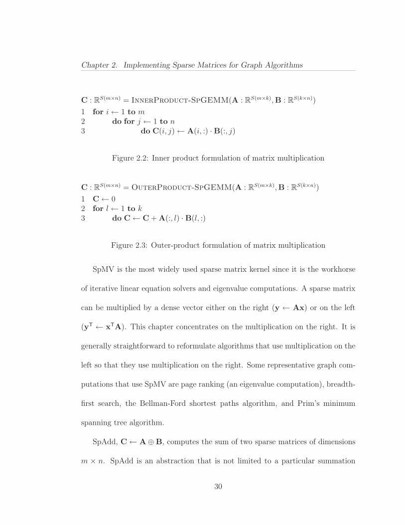
C : RS(m×n) = InnerProduct-SpGEMM(A : R
S(m×k),B : RS(k×n))
1 for i← 1 to m2 do for j ← 1 to n3 do C(i, j)← A(i, :) ·B(:, j)
Figure 2.2: Inner product formulation of matrix multiplication
C : RS(m×n) = OuterProduct-SpGEMM(A : R
S(m×k),B : RS(k×n))
1 C← 02 for l← 1 to k3 do C← C + A(:, l) ·B(l, :)
Figure 2.3: Outer-product formulation of matrix multiplication
SpMV is the most widely used sparse matrix kernel since it is the workhorse
of iterative linear equation solvers and eigenvalue computations. A sparse matrix
can be multiplied by a dense vector either on the right (y ← Ax) or on the left
(yT ← xTA). This chapter concentrates on the multiplication on the right. It is
generally straightforward to reformulate algorithms that use multiplication on the
left so that they use multiplication on the right. Some representative graph com-
putations that use SpMV are page ranking (an eigenvalue computation), breadth-
first search, the Bellman-Ford shortest paths algorithm, and Prim’s minimum
spanning tree algorithm.
SpAdd, C← A⊕B, computes the sum of two sparse matrices of dimensions
m × n. SpAdd is an abstraction that is not limited to a particular summation
30
Chapter 2. Implementing Sparse Matrices for Graph Algorithms
operator. In general, any pointwise binary scalar operation between two sparse
matrices falls into this primitive. Examples include the MIN operator that returns
the minimum of its operands, logical AND, logical OR, ordinary addition, and
subtraction.
SpGEMM computes the sparse product C ← AB, where the input matrices
A ∈ Sm×k and B ∈ S
k×n are both sparse. It is a common operation for operating
on large graphs, used in graph contraction, peer pressure clustering, recursive
formulations of all-pairs-shortest-path algorithms, and breadth-first search from
multiple source vertices. Chapter 3 presents novel ideas for computing SpGEMM.
The computation for matrix multiplication can be organized in several ways.
One common formulation uses inner products, shown in Figure 2.2. Every element
of the product C(i, j) is computed as the dot product of a row i of A and a
column j of B. Another formulation of matrix multiplication uses outer products
(Figure 2.3). The product is computed as a sum of k rank-one matrices. Each
rank-one matrix is the outer product of a column of A with the corresponding
row of B.
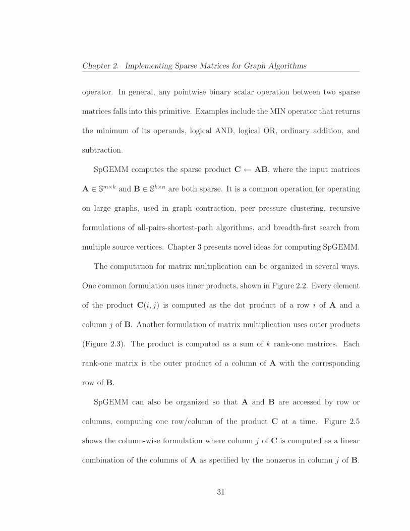
SpGEMM can also be organized so that A and B are accessed by row or
columns, computing one row/column of the product C at a time. Figure 2.5
shows the column-wise formulation where column j of C is computed as a linear
combination of the columns of A as specified by the nonzeros in column j of B.
31
Chapter 2. Implementing Sparse Matrices for Graph Algorithms
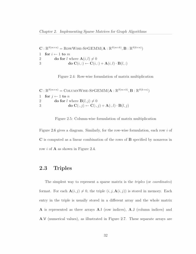
C : RS(m×n) = RowWise-SpGEMM(A : R
S(m×k),B : RS(k×n))
1 for i← 1 to m2 do for l where A(i, l) 6= 03 do C(i, :)← C(i, :) + A(i, l) ·B(l, :)
Figure 2.4: Row-wise formulation of matrix multiplication
C : RS(m×n) = ColumnWise-SpGEMM(A : R
S(m×k),B : RS(k×n))
1 for j ← 1 to n2 do for l where B(l, j) 6= 03 do C(:, j)← C(:, j) + A(:, l) ·B(l, j)
Figure 2.5: Column-wise formulation of matrix multiplication
Figure 2.6 gives a diagram. Similarly, for the row-wise formulation, each row i of
C is computed as a linear combination of the rows of B specified by nonzeros in
row i of A as shown in Figure 2.4.
2.3 Triples
The simplest way to represent a sparse matrix is the triples (or coordinates)
format. For each A(i, j) 6= 0, the triple (i, j,A(i, j)) is stored in memory. Each
entry in the triple is usually stored in a different array and the whole matrix
A is represented as three arrays A.I (row indices), A.J (column indices) and
A.V (numerical values), as illustrated in Figure 2.7. These separate arrays are
32
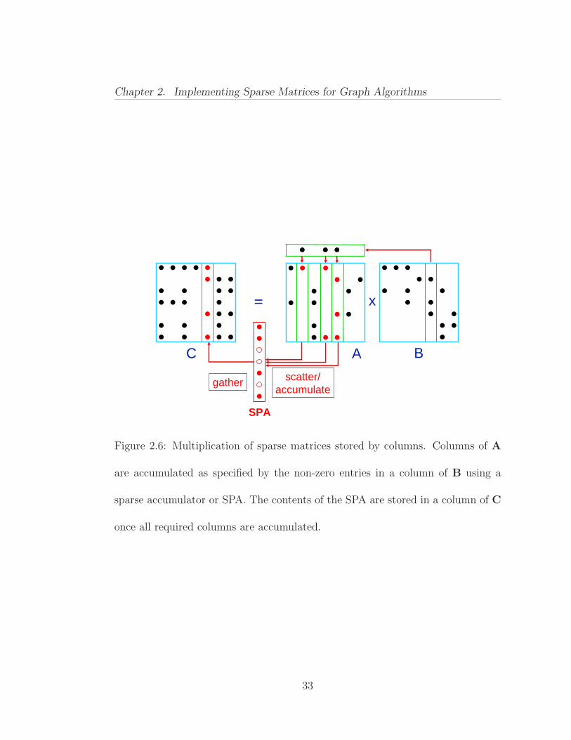
Chapter 2. Implementing Sparse Matrices for Graph Algorithms
B
= x
C A
SPA
gather scatter/ accumulate
Figure 2.6: Multiplication of sparse matrices stored by columns. Columns of A
are accumulated as specified by the non-zero entries in a column of B using a
sparse accumulator or SPA. The contents of the SPA are stored in a column of C
once all required columns are accumulated.
33
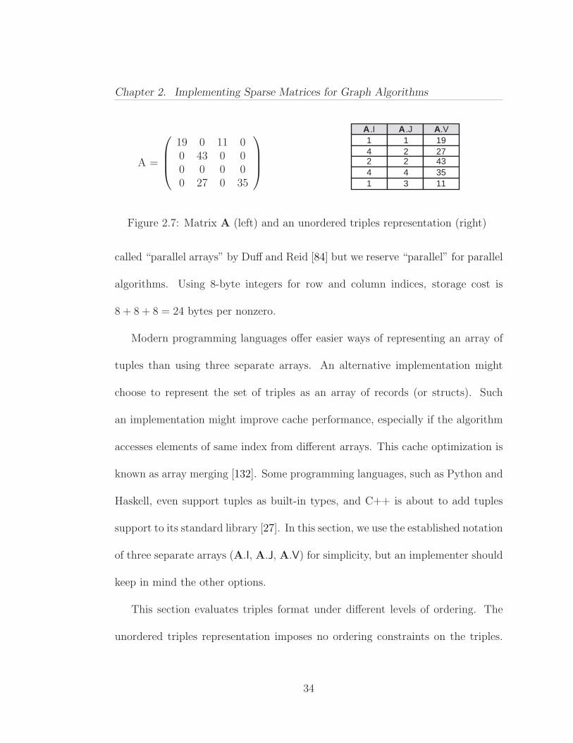
Chapter 2. Implementing Sparse Matrices for Graph Algorithms
A =
19 0 11 00 43 0 00 0 0 00 27 0 35
1 1 194 2 272 2 434 4 351 3 11
A.I A.J A.V
Figure 2.7: Matrix A (left) and an unordered triples representation (right)
called “parallel arrays” by Duff and Reid [84] but we reserve “parallel” for parallel
algorithms. Using 8-byte integers for row and column indices, storage cost is
8 + 8 + 8 = 24 bytes per nonzero.
Modern programming languages offer easier ways of representing an array of
tuples than using three separate arrays. An alternative implementation might
choose to represent the set of triples as an array of records (or structs). Such
an implementation might improve cache performance, especially if the algorithm
accesses elements of same index from different arrays. This cache optimization is
known as array merging [132]. Some programming languages, such as Python and
Haskell, even support tuples as built-in types, and C++ is about to add tuples
support to its standard library [27]. In this section, we use the established notation
of three separate arrays (A.I, A.J, A.V) for simplicity, but an implementer should
keep in mind the other options.
This section evaluates triples format under different levels of ordering. The
unordered triples representation imposes no ordering constraints on the triples.
34
Chapter 2. Implementing Sparse Matrices for Graph Algorithms
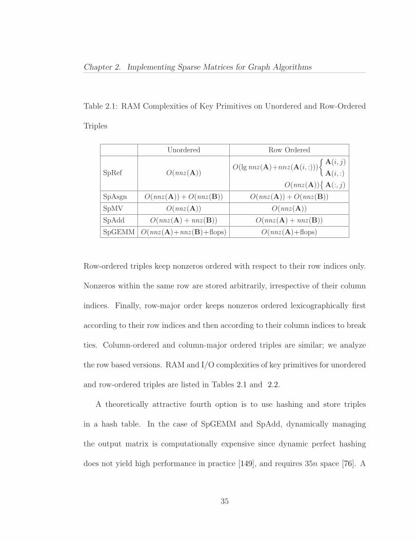
Table 2.1: RAM Complexities of Key Primitives on Unordered and Row-Ordered
Triples
Unordered Row Ordered
SpRef O(nnz (A))O(lg nnz (A)+nnz(A(i, :)))
A(i, j)
A(i, :)
O(nnz (A))
A(:, j)
SpAsgn O(nnz (A)) + O(nnz (B)) O(nnz (A)) + O(nnz (B))
SpMV O(nnz (A)) O(nnz (A))
SpAdd O(nnz (A) + nnz (B)) O(nnz (A) + nnz (B))
SpGEMM O(nnz (A)+nnz (B)+flops) O(nnz (A)+flops)
Row-ordered triples keep nonzeros ordered with respect to their row indices only.
Nonzeros within the same row are stored arbitrarily, irrespective of their column
indices. Finally, row-major order keeps nonzeros ordered lexicographically first
according to their row indices and then according to their column indices to break
ties. Column-ordered and column-major ordered triples are similar; we analyze
the row based versions. RAM and I/O complexities of key primitives for unordered
and row-ordered triples are listed in Tables 2.1 and 2.2.
A theoretically attractive fourth option is to use hashing and store triples
in a hash table. In the case of SpGEMM and SpAdd, dynamically managing
the output matrix is computationally expensive since dynamic perfect hashing
does not yield high performance in practice [149], and requires 35n space [76]. A
35

Chapter 2. Implementing Sparse Matrices for Graph Algorithms
Table 2.2: I/O Complexities of Key Primitives on Unordered and Row-Ordered
Triples
Unordered Row Ordered
SpRef O(scan(A))O(lg nnz (A) + scan(A(i, :))
A(i, j)
A(i, :)
O(scan(A))A(:, j)
SpAsgn O(scan(A) + scan(B)) O(scan(A) + scan(B))
SpMV O(nnz (A)) O(nnz (A))
SpAdd O(nnz (A) + nnz (B)) O(nnz (A) + nnz (B))
SpGEMMO(nnz (A)+nnz (B)+flops)
O(minnnz (A) + flops,
scan(A) lg(nnz (B))+flops)
recently proposed dynamic hashing method called Cuckoo hashing is promising. It
supports queries in worst-case constant time, and updates in amortized expected
constant time, while using only 2n space [157]. Experiments show that it is
substantially faster than existing hashing schemes on modern architectures like
Pentium 4 and IBM Cell [169]. Although hash based schemes seem attractive,
especially for SpAsgn and SpRef primitives [14], further research is required to
test their efficiency for sparse matrix storage.
2.3.1 Unordered Triples
The administrative overhead of the triples representation is low, especially if
the triples are not sorted in any order. With unsorted triples, however, there is
36
Chapter 2. Implementing Sparse Matrices for Graph Algorithms
no spatial locality2 when accessing nonzeros of a given row or column. In the
worst case, all indexing operations might require a complete scan of the data
structure. Therefore, SpRef has O(nnz (A)) RAM complexity and O(scan(A))
I/O complexity.
SpAsgn is no faster either, even though insertions take only constant time per
element. In addition to accessing all the elements of the right hand side matrix
A, SpAsgn also invalidates the existing nonzeros that need to be changed in the
left hand side matrix B. Just finding those triples takes time proportional to the
number of nonzeros in B with unordered triples. Thus, the RAM complexity of
SpAsgn is O(nnz (A)+nnz (B)) and its I/O complexity is O(scan(A)+ scan(B)).
A simple implementation achieving these bounds performs a single scan of B,
outputs only the non-assigned triples (e.g. for B(:, l) = A, those are the triples
(i, j,B(i, j)) where j 6= l), and finally concatenates the nonzeros in A to the
output.
SpMV has full spatial locality when accessing the elements of A, because the
algorithm scans all the nonzeros of A in the exact order that they are stored.
Therefore, O(scan(A)) cache misses are taken for granted as compulsory misses3.
Although SpMV is optimal in the RAM model without any ordering constraints,
2A procedure exploits spatial locality if data that are stored in nearby memory locations arelikely to be referenced close in time
3Assuming that no explicit data prefetching mechanism is used
37
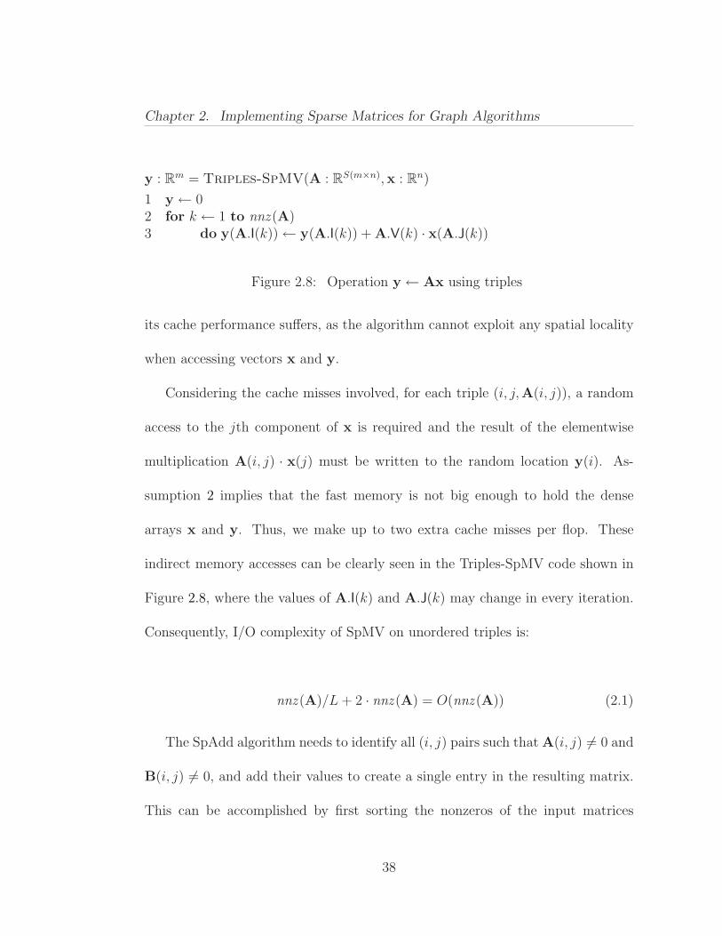
Chapter 2. Implementing Sparse Matrices for Graph Algorithms
y : Rm = Triples-SpMV(A : R
S(m×n),x : Rn)
1 y← 02 for k ← 1 to nnz (A)3 do y(A.I(k))← y(A.I(k)) + A.V(k) · x(A.J(k))
Figure 2.8: Operation y← Ax using triples
its cache performance suffers, as the algorithm cannot exploit any spatial locality
when accessing vectors x and y.
Considering the cache misses involved, for each triple (i, j,A(i, j)), a random
access to the jth component of x is required and the result of the elementwise
multiplication A(i, j) · x(j) must be written to the random location y(i). As-
sumption 2 implies that the fast memory is not big enough to hold the dense
arrays x and y. Thus, we make up to two extra cache misses per flop. These
indirect memory accesses can be clearly seen in the Triples-SpMV code shown in
Figure 2.8, where the values of A.I(k) and A.J(k) may change in every iteration.
Consequently, I/O complexity of SpMV on unordered triples is:
nnz (A)/L + 2 · nnz (A) = O(nnz (A)) (2.1)
The SpAdd algorithm needs to identify all (i, j) pairs such that A(i, j) 6= 0 and
B(i, j) 6= 0, and add their values to create a single entry in the resulting matrix.
This can be accomplished by first sorting the nonzeros of the input matrices
38
Chapter 2. Implementing Sparse Matrices for Graph Algorithms
and then performing a simultaneous scan of sorted nonzeros to sum matching
triples. Using a linear time counting sort, SpAdd is fast in the RAM model with
O(nnz (A) + nnz (B)) complexity.
Counting sort, in its naıve form, has poor cache utilization because the total
size of the counting array is likely to be bigger than the size of the fast memory.
While sorting the nonzeros of a sparse matrix, this translates into one cache
miss per nonzero in the worst case. Therefore, the complexity of SpAdd in the
I/O model becomes O(nnz (A) + nnz (B)). The number of cache misses can be
decreased by using cache optimal sorting algorithms [6] but such algorithms are
comparison based. They do O(n lg n) work as opposed to linear work. Rahman
and Raman [165] give a counting sort algorithm that has better cache utilization
in practice than the naıve algorithm, and still does linear work.
SpGEMM needs fast access to columns, rows, or a given particular element,
depending on the algorithm. One can also think A as a table of i’s and l’s and B
as a table of l’s and j’s; then C is their join [130] on l. This database analogy may
lead to alternative SpGEMM implementations based on ideas from databases. An
outer-product formulation of SpGEMM on unordered triples has three basic steps
(a similar algorithm for general sparse tensor multiplication is given by Bader and
Kolda [15]):
39

Chapter 2. Implementing Sparse Matrices for Graph Algorithms
1. For each l ∈ 1, .., k, identify the set of triples that belong to the lth column
of A, and the lth row of B. Formally, find A(:, l) and B(l, :).
2. For each l ∈ 1, .., k, compute the cartesian product of the row indices of
A(:, l) and the column indices of B(l, :).
Formally, compute the sets Cl = A(:, l).I × B(l, :).J
3. Find the union of all cartesian products, summing up duplicates during set
union: C =⋃
l∈1,..,k Cl
Step 1 of the algorithm can be efficiently implemented by sorting the triples
of A according to their column indices and the triples of B according to their row
indices. Computing the cartesian products in Step 2 takes time
k∑
l=1
nnz (A(:, l)) · nnz (B(l, :)) = flops. (2.2)
Finally, summing up duplicates can be done by lexicographically sorting the ele-
ments from sets Cl. Since there are a total of flops such intermediate triples in
sets Cl for all l, it makes up a total running time of
O(sort(nnz (A)) + sort(nnz (B)) + flops + sort(flops)). (2.3)
As long as the number of nonzeros is more than the dimensions of the matrices
(Assumption 1), it is advantageous to use a linear time sorting algorithm instead
40

Chapter 2. Implementing Sparse Matrices for Graph Algorithms
of a comparison based sort. Since a lexicographic sort is not required for finding
A(:, l) or B(l, :) in Step 1, a single pass of linear time counting sort [68] suffices for
each input matrix. However, two passes of linear time counting sort are required
in Step 3 to produce a lexicographically sorted output. The RAM complexity of
this implementation turns out to be
nnz (A) + nnz (B) + 3 · flops = O(nnz (A) + nnz (B) + flops). (2.4)
However, due to the cache inefficient nature of counting sort, this algorithm
makes O(nnz (A) + nnz (B) + flops) cache misses in the worst case.
Another way to implement SpGEMM on unordered triples is to iterate through
the triples of A. For each (i, j,A(i, j)), we find B(:, j) and multiply A(i, j) by
each nonzero in B(:, j). The duplicate summation step is left intact. The time
this implementation takes is
nnz (A) · nnz (B) + 3 · flops = O(nnz (A) · nnz (B)). (2.5)
The term flops is dominated by the term nnz (A)·nnz (B) according to Theorem 1.
Therefore, the performance is worse than the previous implementation that sorts
the input matrices first.
Theorem 1. For all matrices A and B, flops(AB) ≤ nnz (A) · nnz (B)
Proof. Let the vector of column counts of A be
a = (a1, a2, ..., ak) = (nnz (A(:, 1), nnz (A(:, 2)), ..., nnz (A(:, k))
41
Chapter 2. Implementing Sparse Matrices for Graph Algorithms
and the vector of row counts of B
b = (b1, b2, ..., bk) = (nnz (B(1, :), nnz (B(2, :)), ..., nnz (B(k, :)).
Note that flops = aTb =∑
i=j aibj, and∑
i6=j aibj ≥ 0 as a and b are nonneg-
ative. Consequently,
nnz (A) · nnz (B) = (k∑
l=1
al) · (k∑
l=1
bl) = (∑
i=j
aibj) + (∑
i6=j
aibj)
≥∑
i=j
aibj = aTb = flops
It is worth noting that both implementions of SpGEMM using unordered
triples have O(nnz (A)+nnz (B)+flops) space complexity, due to the intermediate
triples that are all present in the memory after Step 2. Ideally, the space complex-
ity of SpGEMM should be O(nnz (A) + nnz (B) + nnz (C)), which is independent
of flops.
2.3.2 Row-Ordered Triples
The second option is to keep the triplets sorted according to their rows or
columns only. We analyze the row-ordered version; column order is symmet-
ric. This section is divided into three subsections. The first one is on indexing
and SpMV. The second one is on a fundamental abstract data type that is used
42
Chapter 2. Implementing Sparse Matrices for Graph Algorithms
frequently in sparse matrix algorithms, namely the sparse accumulator (SPA).
The SPA is used for implementing some of the SpAdd and SpGEMM algorithms
throughout the rest of this chapter. Finally, the last subsection is on SpAdd and
SpGEMM algorithms.
Indexing and SpMV with Row-Ordered Triples
Using row-ordered triples, indexing still turns out to be inefficient. In practice,
even a fast row access cannot be accomplished, since there is no efficient way
of spotting the beginning of the ith row without using a pointer4. Row-wise
referencing can be done by performing binary search on the whole matrix to
identify a nonzero belonging to the referenced row, and then by scanning in both
directions to find the rest of the nonzeros belonging to that row. Therefore, SpRef
for A(i, :) has O(lg nnz (A) + nnz (A(i, :)) RAM complexity and O(lg nnz (A) +
scan(A(i, :))) I/O complexity. Element-wise referencing also has the same cost,
in both models. Column-wise referencing, on the other hand, is as slow as it was
with unordered triples, requiring a complete scan of the triples.
SpAsgn might incur excessive data movement, as the number of nonzeros in
the left hand side matrix B might change during the operation. For a concrete
example, consider the operation B(i, :) = A where nnz(B(i, :)) 6= nnz (A) before
4That is a drawback of the triples representation in general. The compressed sparse storageformats described in the Section 2.4 provide efficient indexing mechanisms for either rows orcolumns.
43

Chapter 2. Implementing Sparse Matrices for Graph Algorithms
the operation. Since the data structure needs to keep nonzeros with increasing
row indices, all triples with row indices bigger than i need to be shifted by distance
| nnz (A)− nnz (B(i, :))|.
SpAsgn has RAM complexity O(nnz (A))+nnz (B)) and I/O complexity O(1+
scan(A) + scan(B)), where B is the left hand side matrix before the operation.
While implementations of row-wise and element-wise referencing are straightfor-
ward, column-wise referencing (B(:, i) ← A) seems harder as it reduces to a
restricted case of SpAdd, the restriction being that B ∈ S1×n has at most one
nonzero in a given row. Therefore, a similar scanning implementation suffices.
Row-ordered triples format allows an SpMV implementation that makes at
most one extra cache miss per flop. The reason is that references to vector
y show good spatial locality: they are ordered with monotonically increasing
values of A.I(k), avoiding scattered memory referencing on vector y. However,
accesses to vector x are still irregular as the memory stride when accessing x
(|A.J(k + 1) - A.J(k)|) might be as big as the matrix dimension n. Memory
strides can be reduced by clustering the nonzeros in every row. More formally,
this corresponds to reducing the bandwidth of the matrix, which it is defined as:
β(A) = max|i − j| : A(i, j) 6= 0. Toledo [197] experimentally studied differ-
ent methods of reordering the matrix to reduce its bandwidth, along with other
optimizations like blocking and prefetching, to improve the memory performance
44
Chapter 2. Implementing Sparse Matrices for Graph Algorithms
of SpMV. Overall, row ordering does not improve the asymptotic I/O complexity
of SpMV over unordered triples, although it cuts the cache misses by nearly half.
Its I/O complexity becomes
nnz (A)/L + n/L + nnz (A) = O(nnz (A)). (2.6)
The Sparse Accumulator
Most operations that output a sparse matrix generate it one row (or column)
at a time. The current active row is stored temporarily in a special structure
called the sparse accumulator (SPA) [104] (or expanded real accumulator [163]).
The SPA helps merging unordered lists in linear time.
There are different ways of implementing the SPA as it is an abstract data type,
not a concrete data structure. In our SPA implementation, w is the dense vector
of values, b is the boolean dense vector that contains “occupied” flags, and LS is
the list that keeps an unordered list of indices, as Gilbert et al. described [104].
Scatter-SPA function, given in Figure 2.9, adds a scalar (value) to a specific
position (pos) of the SPA. Scattering is a constant time operation. Gathering the
SPA’s nonzeros to the output matrix C takes O(nnz (SPA)) time. The pseudocode
for the Gather-SPA is given in Figure 2.10. It is crucial to initialize the SPA only
once at the beginning, as this takes O(n) time. Resetting it later for the next
45
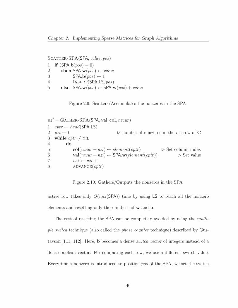
Chapter 2. Implementing Sparse Matrices for Graph Algorithms
Scatter-SPA(SPA, value, pos)
1 if (SPA.b(pos) = 0)2 then SPA.w(pos)← value3 SPA.b(pos)← 14 Insert(SPA.LS, pos)5 else SPA.w(pos)← SPA.w(pos) + value
Figure 2.9: Scatters/Accumulates the nonzeros in the SPA
nzi = Gather-SPA(SPA,val, col, nzcur)
1 cptr ← head(SPA.LS)2 nzi ← 0 number of nonzeros in the ith row of C3 while cptr 6= nil
4 do5 col(nzcur + nzi)← element(cptr) Set column index6 val(nzcur + nzi)← SPA.w(element(cptr)) Set value7 nzi ← nzi +18 advance(cptr)
Figure 2.10: Gathers/Outputs the nonzeros in the SPA
active row takes only O(nnz (SPA)) time by using LS to reach all the nonzero
elements and resetting only those indices of w and b.
The cost of resetting the SPA can be completely avoided by using the multi-
ple switch technique (also called the phase counter technique) described by Gus-
tavson [111, 112]. Here, b becomes a dense switch vector of integers instead of a
dense boolean vector. For computing each row, we use a different switch value.
Everytime a nonzero is introduced to position pos of the SPA, we set the switch
46

Chapter 2. Implementing Sparse Matrices for Graph Algorithms
C : RS(m×n) = RowTriples-SpAdd(A : R
S(m×n),B : RS(m×n))
1 Set-SPA(SPA) Set w = 0, b = 0 and create empty list LS
2 ka← kb← kc← 1 Initialize current indices to one3 for i← 1 to m4 do while (ka ≤ nnz (A) and A.I(ka) = i)5 do Scatter-SPA(SPA,A.V(ka),A.J(ka))6 ka← ka + 17 while (kb ≤ nnz (B) and B.I(kb) = i)8 do Scatter-SPA(SPA,B.V(kb),B.J(kb))9 kb← kb + 1
10 nznew ← Gather-SPA(SPA,C.V,C.J, kc)11 for j ← 0 to nznew −112 do C.I(kc + j)← i Set row index13 kc← kc + nznew14 Reset-SPA(SPA) Reset w = 0, b = 0 and empty LS
Figure 2.11: Operation C← A⊕B using row-ordered triples
to the current active row index (SPA.b(pos) ← i). During the computation of
subsequent rows j = i + 1, ...,m, the switch value being less than the current
active row index (SPA.b(pos) ≤ j) means that the position pos of the SPA is
“free”. Therefore, the need to reset b for each row is avoided.
SpAdd and SpGEMM with Row-Ordered Triples
Using the SPA, we can implement SpAdd with O(nnz (A) + nnz (B)) RAM
complexity. The full procedure is given in Figure 2.11. The I/O complexity of
this SpAdd implementation is also O(nnz (A) + nnz (B)). This is because for
each nonzero scanned from inputs, the algorithm checks and updates an arbitrary
47

Chapter 2. Implementing Sparse Matrices for Graph Algorithms
position of the SPA. From Assumption 2, these arbitrary accesses are likely to
incur cache misses every time.
It is possible to implement SpGEMM using the same outer-product formula-
tion described in Section 2.3.1, with a slightly better asymptotic RAM complexity
of O(nnz(A)+flops), as the triples of B are already sorted according to their row
indices. Instead, we describe a row-wise implementation, similar to the CSR based
algorithm described in Section 2.4. Due to inefficient row-wise indexing support of
row-ordered triples, however, the operation count is higher than the CSR version.
A SPA of size n is used to accumulate the nonzero structure of the current active
row of C. A direct scan of the nonzeros of A allows enumeration of nonzeros in
A(i, :) for increasing values of i ∈ 1, ..,m. Then, for each triple (i, l,A(i, l))
in the ith row of A, the matching triples (l, j,B(l, j)) of the lth row of B need
to be found using the SpRef primitive. This way, the nonzeros in C(i, :) are ac-
cumulated. The whole procedure is given in Figure 2.12. Its RAM complexity
is
∑
A(i,l) 6=0
(nnz (B(i, :)) lg(nnz (B))
)+ flops = O(nnz (A) lg(nnz (B)) + flops) (2.7)
where the lg nnz (B) factor per each nonzero in A comes from the row-wise SpRef
operation in line 5. Its I/O complexity is
O(scan(A) lg(nnz (B)) + flops). (2.8)
48

Chapter 2. Implementing Sparse Matrices for Graph Algorithms
C : RS(m×n) = RowTriples-SpGEMM(A : R
S(m×k),B : RS(k×n))
1 Set-SPA(SPA) Set w = 0, b = 0 and create empty list LS
2 ka← kc← 1 Initialize current indices to one3 for i← 1 to m4 do while (ka ≤ nnz (A) and A.I(ka) = i)5 do BR← B(A.J(ka), :) Using SpRef6 for kb← 1 to nnz (BR)7 do value ← A.NUM(ka) ·BR.NUM(kb)8 Scatter-SPA(SPA, value,BR.J(kb))9 ka← ka + 1
10 nznew ← Gather-SPA(SPA,C.V,C.J, kc)11 for j ← 0 to nznew −112 do C.I(kc + j)← i Set row index13 kc← kc + nznew14 Reset-SPA(SPA) Reset w = 0, b = 0 and empty LS
Figure 2.12: Operation C← AB using row-ordered triples
While the complexity of row-wise implementation is asymptotically worse than
the outer-product implementation in the RAM model, it has the advantage of
using only O(nnz (C)) space as opposed to the O(flops) space used by the outer-
product implementation. On the other hand, the I/O complexities of the outer-
product version and the row-wise version are not directly comparable. Which one
is faster depends on the cache line size and the number of nonzeros in B.
49
Chapter 2. Implementing Sparse Matrices for Graph Algorithms
2.3.3 Row-Major Ordered Triples
We now consider the third option of storing triples in lexicographic order,
either in column-major or row-major order. Once again, we focus on the row
oriented scheme.
In order to reference a whole row, binary search on the whole matrix, followed
by a scan on both directions is used, as with row-ordered triples. As the nonzeros
in a row are ordered by column indices, it seems there should be a faster way to
access a single element than the method used on row-ordered triples. A faster way
indeed exists but ordinary binary search would not do it, because the beginning
and the end of the ith row is not known in advance. The algorithm has three
steps:
1. Spot a triple (i, j,A(i, j)) that belongs to the ith row by doing binary search
on the whole matrix
2. From that triple, perform an unbounded binary search [147] in both direc-
tions. In an unbounded search, the step length is doubled at each iteration.
The search terminates at a given direction when it hits a triple that does not
belong to the ith row. Those two triples (one from each direction) becomes
the boundary triples.
50

Chapter 2. Implementing Sparse Matrices for Graph Algorithms
11
90
11
76
12
57
12
89
12
19
12
96
12
65
12
44
12
34
13
21
13
11
13
54
10
31
12
28
12
28
5 12 2 3 4 7 10 11 13 2 9 1118 16 18
A.I
A.J
A.V
Step 2
Step 3
Figure 2.13: Element-wise indexing of A(12, 16) on row-major ordered triples
3. Perform ordinary binary search within the exclusive range defined by the
boundary vertices.
The number of total operations is O(lg nnz (A) + lg nnz (A(i, :)) = O(lg nnz (A)).
An example is given in Figure 2.13.
While unbounded binary search is the preferred method in the RAM model,
simple scanning might be faster in the I/O model. Searching an element in an
ordered set of n elements can be achieved with Θ(logL n) cost in the I/O model,
using B-trees [26]. However, using an ordinary array, search incurs lg n cache
misses. This may or may not be less than scan(n). Therefore, we define the cost
of searching within an ordered row as follows:
search(A(i, :)) = minlg nnz (A(i, :)), scan(A(i, :)) (2.9)
51
Chapter 2. Implementing Sparse Matrices for Graph Algorithms
For column-wise referencing as well as for SpAsgn operations, row-major or-
dered triples format does not provide any improvement over row-ordered triples.
In SpMV, the only array that does not show excellent spatial locality is x,
since A.I,A.J,A.V, and y are accessed with mostly consecutive, increasing index
values. Accesses to x are also with increasing indices, which is an improvement
over row-ordered triples. However, memory strides when accessing x can still be
high, depending on the number of nonzeros in each row and the bandwidth of the
matrix. In the worst case, each access to x might incur a cache miss.
Bender et al. [28] came up with cache-optimal algorithms for SpMV using
the column-major layout. From a high-level view, their method first generates all
the intermediate triples of y, possibly with repeating indices. Then, the algorithm
sorts those intermediate triples with respect to their row indices, performing addi-
tions on the triples with same row index on the fly. I/O optimality of their SpMV
algorithm relies on the existence of an I/O optimal sorting algorithm. Their com-
plexity measure assumes a fixed k number of nonzeros per column, leading to I/O
complexity of
O
(scan(A) logZ/L
n
maxZ, k
). (2.10)
SpAdd is now more efficient even without using any auxiliary data structure. A
scan-based array merging algorithm is sufficient as long as we sum duplicates while
52

Chapter 2. Implementing Sparse Matrices for Graph Algorithms
Table 2.3: RAM Complexities of Key Primitives on Row-Major Ordered Triples
and CSR
Row-Major Ordered Triples CSR
SpRef
O(lg nnz (A))A(i, j) O(lg nnz (A(i, :))
A(i, j)
O(lg nnz (A) + nnz (A(i, :))
A(i, :) O(nnz (A(i, :))
A(i, :)
O(nnz (A))A(:, j) O(nnz (A))
A(:, j)
SpAsgn O(nnz (A) + nnz (B)) O(nnz (A) + nnz (B))
SpMV O(nnz (A)) O(nnz (A))
SpAdd O(nnz (A) + nnz (B)) O(nnz (A) + nnz (B))
SpGEMM O(nnz (A)+flops) O(nnz (A)+flops)
merging. Such an implementation has O(nnz (A)+nnz (B)) RAM complexity and
O(scan(A) + scan(B)) I/O complexity5.
Row-major ordered triples allow outer-product and row-wise SpGEMM im-
plementations at least as efficiently as row-ordered triples. Indeed, some finer
improvements are possible by exploiting the more specialized structure. In the
case of row-wise SpGEMM, a technique called finger search [43] can be used to
improve the RAM complexity. While enumerating all triples (i, l,A) ∈ A(i, :),
they are naturally sorted with increasing l values. Therefore, accesses to B(l, :)
are also with increasing l values. Instead of restarting the binary search from the
beginning of B, one can use fingers and only search the yet unexplored subse-
5These bounds are optimal only if nnz (A) = Θ(nnz (B)) [46]
53
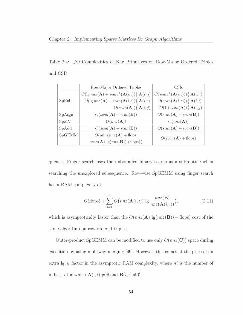
Chapter 2. Implementing Sparse Matrices for Graph Algorithms
Table 2.4: I/O Complexities of Key Primitives on Row-Major Ordered Triples
and CSR
Row-Major Ordered Triples CSR
SpRef
O(lg nnz (A) + search(A(i, :))
A(i, j) O(search(A(i, :)))A(i, j)
O(lg nnz (A) + scan(A(i, :))
A(i, :) O(scan(A(i, :)))A(i, :)
O(scan(A))A(:, j) O(1+scan(A))
A(:, j)
SpAsgn O(scan(A) + scan(B)) O(scan(A) + scan(B))
SpMV O(nnz (A)) O(nnz (A))
SpAdd O(scan(A) + scan(B)) O(scan(A) + scan(B))
SpGEMM O(minnnz (A) + flops,O(scan(A) + flops)
scan(A) lg(nnz (B))+flops)
quence. Finger search uses the unbounded binary search as a subroutine when
searching the unexplored subsequence. Row-wise SpGEMM using finger search
has a RAM complexity of
O(flops) +n∑
i=1
O(nnz (A(i, :)) lg
nnz (B)
nnz (A(i, :))
), (2.11)
which is asymptotically faster than the O(nnz (A) lg(nnz (B)) + flops) cost of the
same algorithm on row-ordered triples.
Outer-product SpGEMM can be modified to use only O(nnz (C)) space during
execution by using multiway merging [49]. However, this comes at the price of an
extra lg ni factor in the asymptotic RAM complexity, where ni is the number of
indices i for which A(:, i) 6= ∅ and B(i, :) 6= ∅.
54
Chapter 2. Implementing Sparse Matrices for Graph Algorithms
Although both of these refined algorithms are asymptotically slower than the
naive outer-product method, they might be faster in practice because of the cache
effects and difference in constants in the asymptotic complexities. Further research
is required in algorithm engineering of SpGEMM to find the best performing
algorithm in real life. Chapter 3 includes extensive experiments, for two new
SpGEMM algorithms, under various settings.
2.4 Compressed Sparse Row/Column
The most widely used storage schemes for sparse matrices are compressed
sparse column (CSC) and compressed sparse row (CSR). For example, Matlab
uses CSC format to store its sparse matrices [104]. Both are dense collections
of sparse arrays. We examine CSR, which is introduced by Gustavson under the
name of sparse row-wise representation [110]; CSC is symmetric.
CSR can be seen as a concatenation of sparse row arrays. On the other hand,
it is also very close to row-ordered triples, with an auxiliary index of size Θ(n).
In this section, we assume that nonzeros within each sparse row array are ordered
with increasing row indices. This is not a general requirement though. Davis’s
CSparse package [74], for example, does not impose any ordering within the sparse
arrays.
55
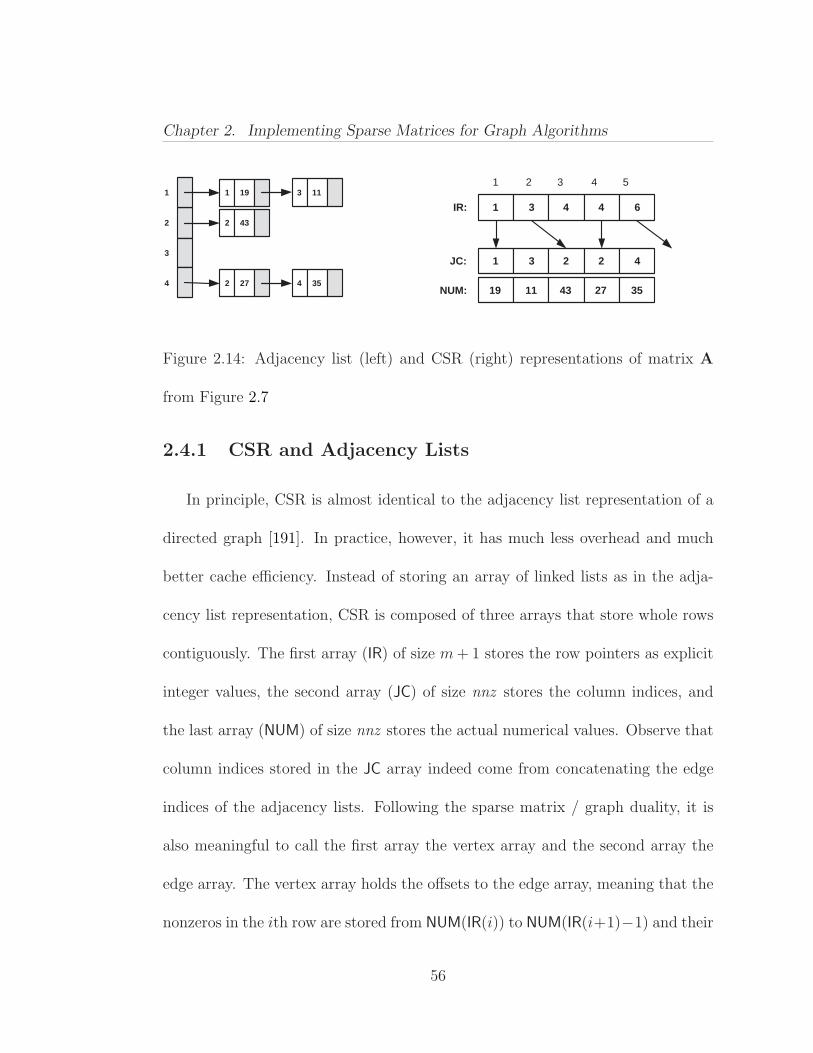
Chapter 2. Implementing Sparse Matrices for Graph Algorithms
1
2
3
4
1 19 3 11
2 43
4 35 2 27
1 3 4 4 6
1 3 2 2 4
19 11 43 27 35
IR:
JC:
NUM:
1 2 3 4 5
Figure 2.14: Adjacency list (left) and CSR (right) representations of matrix A
from Figure 2.7
2.4.1 CSR and Adjacency Lists
In principle, CSR is almost identical to the adjacency list representation of a
directed graph [191]. In practice, however, it has much less overhead and much
better cache efficiency. Instead of storing an array of linked lists as in the adja-
cency list representation, CSR is composed of three arrays that store whole rows
contiguously. The first array (IR) of size m + 1 stores the row pointers as explicit
integer values, the second array (JC) of size nnz stores the column indices, and
the last array (NUM) of size nnz stores the actual numerical values. Observe that
column indices stored in the JC array indeed come from concatenating the edge
indices of the adjacency lists. Following the sparse matrix / graph duality, it is
also meaningful to call the first array the vertex array and the second array the
edge array. The vertex array holds the offsets to the edge array, meaning that the
nonzeros in the ith row are stored from NUM(IR(i)) to NUM(IR(i+1)−1) and their
56

Chapter 2. Implementing Sparse Matrices for Graph Algorithms
respective positions within that row are stored from JC(IR(i)) to JC(IR(i+1)−1).
Also note that JC(i) = JC(i + 1) means there are no nonzeros in the ith row.
Figure 2.4.1 shows the adjacency list and CSR representations of matrix A
from Figure 2.7 . While the arrows in the adjacency based representation are
actual pointers to memory locations, the arrows in CSR are not. The edge array
offsets are actually (unsigned) integers.
The efficiency advantage of the CSR data structure as compared with the
adjacency list can be explained by the memory architecture of modern comput-
ers. In order to access all the nonzeros in a given row i, which is equivalent
to traversing all the outgoing edges of a given vertex vi, CSR makes at most
⌈nnz (A(i, :))/L⌉ cache misses. A similar access to the adjacency list representa-
tion incurs nnz (A(i, :)) cache misses in the worst case, worsening as the memory
becomes more and more fragmented. In an experiment published in 1998, Black
et al. [31] found out that an array based representation was 10 times faster to
traverse than a linked-list based representation. This performance gap is due to
the high cost of pointer chasing that happens frequently in linked data structures.
The efficiency of CSR comes at a price though: introducing new nonzero elements
or deleting a nonzero element is computationally inefficient [104]. Therefore, CSR
is best suited for representing static graphs. The only one of our key primitives
that changes the graph is SpAsgn.
57
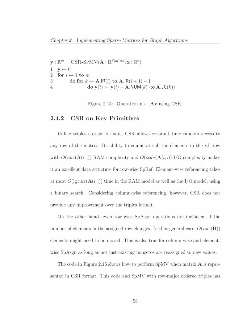
Chapter 2. Implementing Sparse Matrices for Graph Algorithms
y : Rm = CSR-SpMV(A : R
S(m)×n,x : Rn)
1 y← 02 for i← 1 to m3 do for k ← A.IR(i) to A.IR(i + 1)− 14 do y(i)← y(i) + A.NUM(k) · x(A.JC(k))
Figure 2.15: Operation y← Ax using CSR
2.4.2 CSR on Key Primitives
Unlike triples storage formats, CSR allows constant time random access to
any row of the matrix. Its ability to enumerate all the elements in the ith row
with O(nnz (A(i, :)) RAM complexity and O(scan(A(i, :)) I/O complexity makes
it an excellent data structure for row-wise SpRef. Element-wise referencing takes
at most O(lg nnz (A(i, :)) time in the RAM model as well as the I/O model, using
a binary search. Considering column-wise referencing, however, CSR does not
provide any improvement over the triples format.
On the other hand, even row-wise SpAsgn operations are inefficient if the
number of elements in the assigned row changes. In that general case, O(nnz (B))
elements might need to be moved. This is also true for column-wise and element-
wise SpAsgn as long as not just existing nonzeros are reassigned to new values.
The code in Figure 2.15 shows how to perform SpMV when matrix A is repre-
sented in CSR format. This code and SpMV with row-major ordered triples has
58
Chapter 2. Implementing Sparse Matrices for Graph Algorithms
similar performance characteristics except for a few subtleties. When some rows
of A are all zeros, those rows are effectively skipped in row-major ordered triples,
but still need to be examined in CSR. On the other hand, when m << nnz , CSR
has a clear advantage since it needs to examine only one index (A.JC(k)) per
inner loop iteration while row-major ordered triples needs to examine two (A.I(k)
and A.J(k)). This may make up to a factor of two difference in the number of
cache misses. CSR also has some advantages over CSC when the SpMV primitive
is considered (expecially in the case of y← y + Ax), as experimentally shown by
Vuduc [206].
Blocked versions of CSR and CSC try to take advantage of clustered nonzeros
in the sparse matrix. While blocked CSR (BCSR) achieves superior performance
for SpMV on matrices resulting from finite element meshes [206] mostly by using
loop unrolling and register blocking, it is of little use when the matrix itself does
not have its nonzeros clustered. Pinar and Heath proposed a reordering mecha-
nism to cluster those nonzeros to get dense subblocks [162]. However, it is not
clear whether such mechanisms are successful for highly irregular matrices from
sparse real world graphs.
Except for the additional bookkeeping required for getting the row pointers
right, SpAdd can be implemented in the same way as with row-major ordered
59
Chapter 2. Implementing Sparse Matrices for Graph Algorithms
triples. The extra bookkeeping of row pointers does not affect the asymptotic
complexity.
One subtlety overlooked in the SpAdd implementations throughout this chap-
ter is management of the memory required by the resulting matrix C. We implic-
itly assumed that the data structure holding C has enough space to accommodate
all of its elements. Repeated doubling of memory whenever necessary is one way
of addressing this issue. Another conservative way is to reserve nnz (A) + nnz (B)
space for C at the beginning of the procedure and shrink any unused portion after
the computation, right before the procedure returns.
The efficiency of accessing and enumerating rows in CSR makes the row-wise
SpGEMM formulation, described in Figure 2.4, the preferred matrix multiplica-
tion formulation. An efficient implementation of the row-wise SPGEMM using
CSR was first given by Gustavson [113]. It had a RAM complexity of
O(m + n + nnz (A) + flops) = O(nnz (A) + flops), (2.12)
where the equality follows from Assumption 1. Recent column-wise implemen-
tations with similar RAM complexities are provided by Davis in his CSparse
software [74] and by Matlab [104]. The algorithm, presented in Figure 2.16 uses
the sparse accumulator (SPA) described in Section 2.3.2. Once again, the multi-
ple switch technique can be used to avoid the cost of resetting the SPA for every
60

Chapter 2. Implementing Sparse Matrices for Graph Algorithms
C : RS(m)×n = CSR-SpGEMM(A : R
S(m)×k,B : RS(k)×n)
1 Set-SPA(SPA) Set w = 0, b = 0 and create empty list LS
2 C.IR(1)← 03 for i← 1 to m4 do for k ← A.IR(i) to A.IR(i + 1)5 do for j ← B.IR(A.JC(k)) to B.IR(A.JC(k) + 1)6 do7 value ← A.NUM(k) ·B.NUM(j)8 Scatter-SPA(SPA, value,B.JC(j))9 nznew ← Gather-SPA(SPA,C.NUM,C.JC,C.IR(i))
10 C.IR(i + 1)← C.IR(i) + nznew11 Reset-SPA(SPA) Reset w = 0, b = 0 and empty LS
Figure 2.16: Operation C← AB using CSR
iteration of the outermost loop. As in the case of SpAdd, generally the space
required to store C cannot be determined quickly. Repeated doubling or more
sophisticated methods such as Cohen’s algorithm [63] may be used. Cohen’s algo-
rithm is a randomized iterative algorithm that does Θ(1) SpMV operations over a
semiring to estimate the row and column counts. It can be efficiently implemented
even on unordered triples.
The row-wise SpGEMM implementation does O(scan(A)+flops) cache misses
in the worst case. Due to the size of the SPA and Assumption 2, the algorithm
makes a cache miss for every flop. As long as no cache interference occurs between
the nonzeros of A and the nonzeros of C(i, :), only scan(A) additional cache misses
are made instead of nnz (A).
61
Chapter 2. Implementing Sparse Matrices for Graph Algorithms
2.5 Other Related Work and Conclusion
In this chapter, we gave a brief survey of sparse matrix infrastructure for doing
graph algorithms. We focused on implementation and analysis of key primitives
using various standard sparse matrix data structures. We tried to complement
the existing literature in two directions. First, we analyzed sparse matrix indexing
and assignment operations. Second, we gave I/O complexity bounds for all oper-
ations. Taking I/O complexies into account is key to achieving high performance
on modern architectures with multiple levels of cache.
A vast literature exists on sparse matrix storage schemes. We tried to cover
the most general ones in this chapter. There are specialized data structures that
perform certain computations more efficiently. For example:
• Blocked compressed stripe formats (BCSR and BCSC) [122] uses less band-
width to accelerate bandwidth limited computations such as SpMV.
• Knuth storage [128] allows fast access to both rows and columns at the same
time, and it makes dynamic changes to the matrix possible. Therefore, it is
very suitable for all kinds of SpRef and SpAsgn operations. Its drawback is
its excessive memory usage (5 nnz +2n) and high cache miss ratio.
• Hierarchical storage schemes such as quadtrees [173, 209] are theoretically
attractive, but achieving good performance in practice requires careful al-
62

Chapter 2. Implementing Sparse Matrices for Graph Algorithms
gorithm engineering to avoid high cache miss ratios that would result from
straightforward pointer based implementations.
• Parallel data structures that are designed for multithreaded executions are
becoming attractive with the multicore revolution. Our Compressed Sparse
Blocks (CSB) format, introduced in Section 6 guarantees plenty of paral-
lelism for multithreaded SpMV and SpMV T (sparse matrix-transpose-dense
vector multiplication) computations.
63
Chapter 3
New Ideas in SparseMatrix-Matrix Multiplication
Part of the material in this chapter previously appeared in preliminary form in
papers by Buluc and Gilbert that appeared in the proceedings of IPDPS’08 [49]
and ICPP’08 [48].
3.1 Introduction
Development and implementation of large-scale parallel graph algorithms poses
numerous challenges in terms of scalability and productivity [143, 210]. Lin-
ear algebra formulations of many graph algorithms already exist in the litera-
ture [7, 146, 192]. By exploiting the duality between matrices and graphs, linear
algebraic formululations aim to apply the existing knowledge on parallel matrix
algorithms to parallel graph algorithms. One of the key primitives in array-based
64
Chapter 3. New Ideas in Sparse Matrix-Matrix Multiplication
graph algorithms is computing the product of two sparse matrices (SpGEMM) over
a semiring. Sparse matrix-matrix multiplication is a building block for many algo-
rithms including graph contraction [105], breadth-first search from multiple source
vertices, peer pressure clustering [180], recursive formulations of all-pairs shortest-
paths algorithms [71], matching algorithms [164], and cycle detection [211], as well
as for some other applications such as multigrid interpolation/restriction [42], and
parsing context-free languages [161].
Most large graphs in applications, such as the WWW graph, finite element
meshes, planar graphs, and trees, are sparse. In this work, we consider a graph
to be sparse if nnz = O(n), where nnz is the number of edges and n is the
number of vertices. Dense matrix multiplication algorithms are inefficient for
SpGEMM since they require O(n3) space and the current fastest dense matrix
multiplication algorithm runs in O(n2.38) [67, 177] time. Furthermore, fast dense
matrix multiplication algorithms operate on a ring instead of a semiring, which
makes them unsuitable for many algorithms on general graphs. For example,
it is possible to embed the semiring into the ring of integers for the all-pairs
shortest-paths problem on unweighted and undirected graphs [177], but the same
embedding does not work for weighted or directed graphs [213].
The previous chapter explains CSC/CSR, the most widely used data struc-
tures for sparse matrices, in detail. It also gives concise descriptions of common
65
Chapter 3. New Ideas in Sparse Matrix-Matrix Multiplication
SpGEMM algorithms operating both on CSC/CSR and triples. The SpGEMM
problem was recently reconsidered by Yuster and Zwick [212] over a ring, where
the authors use a fast dense matrix multiplication such as arithmetic progres-
sion [67] as a subroutine. Their algorithm uses O(nnz 0.7 n1.2 + n2+o(1)) arithmetic
operations, which is theoretically close to optimal only if we assume that the
number of nonzeros in the resulting matrix C is Θ(n2). This assumption rarely
holds in reality. Instead, we provide a work sensitive analysis by expressing the
computation complexity of our SpGEMM algorithms in terms of flops.
Practical sparse algorithms have been proposed by different researchers over
the years [159, 189] using various data structures. Although they achieve reason-
able performance on some classes of matrices, none of these algorithms outper-
forms the classical sparse matrix-matrix multiplication algorithm, which was first
described by Gustavson [113] and was used in Matlab [104] and CSparse [74]. The
classical algorithm runs in O(flops + nnz +n) time.
In Section 3.2, we present two novel algorithms for sequential SpGEMM. The
first one is geared towards computing the product of two hypersparse matrices.
A matrix is hypersparse if the ratio of nonzeros to its dimension is asymptoti-
cally 0. It is used as the sequential building block of our parallel 2D algorithms de-
scribed in Section 3.3. Our Hypersparse GEMM algorithm uses a new O(nnz )
data structure, called DCSC for doubly compressed sparse columns , which
66
Chapter 3. New Ideas in Sparse Matrix-Matrix Multiplication
is explained in Section 3.2.1. The Hypersparse GEMM is based on the outer-
product formulation and has time complexity O(nzc(A) + nzr(B) + flops · lg ni),
where nzc(A) is the number of columns of A that contain at least one nonzero,
nzr(B) is the number of rows of B that contain at least one nonzero, and ni is the
number of indices i for which A(:, i) 6= ∅ and B(i, :) 6= ∅. The overall space com-
plexity of our algorithm is only O(nnz (A) + nnz (B) + nnz (C)). Notice that the
time complexity of our algorithm does not depend on n, and the space complexity
does not depend on flops.
The second sequential algorithm is an ordered variant of the column-by-column
formulation, and has better expected time complexity for random matrices, but
worse worst-case time complexity in general. It is specifically geared towards
matrices with dimensions large enough to force a single dense column not to fit in
cache. It works on any sparse matrix data structure that can enumerate nonzeros
in the jth column in O(nnz (j)) time. We include a preliminary experimental
evaluation of the column-by-column algorithm in this section, comparing it with
the classical algorithm.
Section 3.3 presents parallel algorithms for SpGEMM. We propose novel algo-
rithms based on 2D block decomposition of data in addition to giving the complete
description of an existing 1D algorithm. To the best of our knowledge, parallel
67
Chapter 3. New Ideas in Sparse Matrix-Matrix Multiplication
algorithms using a 2D block decomposition have not earlier been developed for
sparse matrix-matrix multiplication.
Toledo et al. [123] proved that 2D dense matrix multiplication algorithms are
optimal with respect to the communication volume, making 2D sparse algorithms
likely to be more scalable than their 1D counterparts. In Section 3.4, we show that
this intuition is indeed correct by providing a theoretical analysis of the parallel
performance of 1D and 2D algorithms.
In Section 3.5, we model the speedup of parallel SpGEMM algorithms using
realistic simulations and projections. Our results show that existing 1D algorithms
are not scalable to thousands of processors. By contrast, 2D algorithms have the
potential for scaling up indefinitely, albeit with decreasing parallel efficiency, which
is defined as the ratio of speedup to the number of processors.
Section 3.6 describes the experimental setup we used for evaluating our Sparse
SUMMA implementation, and presents the final results. We describe other tech-
niques we have used for implementating our parallel algorithms, and their effects
on performance in Section 3.7. Section 3.8 offers some future directions.
68
Chapter 3. New Ideas in Sparse Matrix-Matrix Multiplication
3.2 Sequential Sparse Matrix Multiply
In this section, we first analyze different formulations of sparse matrix-matrix
multiplication using the layered graph model. We present our Hypersparse GEMM
algorithm in Section 3.2.1. Finally, we present our cache-efficient column-by-
column algorithm in Section 3.2.2 together with its experimental evaluation.
Matrix multiplication can be organized in many different ways. The inner-
product formulation that usually serves as the definition of matrix multiplication
is well-known. Given two matrices A ∈ Rm×k and B ∈ R
k×n, each element in the
product C ∈ Rm×n is computed by the following formula:
C(i, j) =k∑
l=1
A(i, l)B(l, j). (3.1)
This formulation is rarely useful for multiplying sparse matrices since it re-
quires Ω(mn) operations regardless of the sparsity of the operands.
We represent the multiplication of two matrices A and B as a three layered
graph, following Cohen [63]. The layers have m, k and n vertices, in that order.
The first layer of vertices (U) represent the rows of A and the third layer of vertices
(V ) represent the columns of B. The second layer of vertices (W ) represent the
dimension shared between matrices. Every nonzero A(i, l) 6= 0 in the ith row of
A forms an edge (ui, wl) between the first and second layers and every nonzero in
69
Chapter 3. New Ideas in Sparse Matrix-Matrix Multiplication
B(l, j) 6= 0 in the jth column of B forms an edge (wl, vj) between the second and
third layers.
We perform different operations on the layered graph depending on the way
we formulate the multiplication. In all cases though, the goal is to find pairs of
vertices (ui, vj) sharing an adjacent vertex wk ∈ W , and if any pair shares multiple
adjacent vertices, to merge their contributions.
Using inner products, we analyze each pair (ui, vj) to find the set of vertices
in Wij ⊆ W = w1, w2, ..., wk that are connected to both ui amd vj in the graph
shown in Figure 3.1. The algorithm then accumulates contributions ail · blj for all
wl ∈ Wij. The result becomes the value of C(i, j) in the output. In general this
inner-product subgraph is sparse, and a contribution from wl happens only when
both edges ail and blj exist. However, this sparsity is not exploited using inner
products as it needs to examine each (ui, vj) pair, even when the set Wij is empty.
In the outer-product formulation, the product is written as the summation of
k rank one matrices:
C =k∑
l=1
A(:, l)B(l, :). (3.2)
A different subgraph results from this formulation as it is the set of vertices
W that represent the shared dimension that play the central role. Note that
the edges are traversed in the outward direction from a node wi ∈ W , as shown
in Figure 3.2. For sufficiently sparse matrices, this formulation may run faster
70
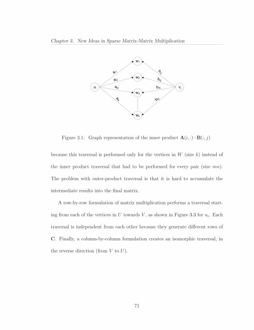
Chapter 3. New Ideas in Sparse Matrix-Matrix Multiplication
ui
w2
w1
w3
wk
vj
a i1
ai2
ai3
aik
b1j
b2j
b3j
b kj
Figure 3.1: Graph representation of the inner product A(i, :) ·B(:, j)
because this traversal is performed only for the vertices in W (size k) instead of
the inner product traversal that had to be performed for every pair (size mn).
The problem with outer-product traversal is that it is hard to accumulate the
intermediate results into the final matrix.
A row-by-row formulation of matrix multiplication performs a traversal start-
ing from each of the vertices in U towards V , as shown in Figure 3.3 for ui. Each
traversal is independent from each other because they generate different rows of
C. Finally, a column-by-column formulation creates an isomorphic traversal, in
the reverse direction (from V to U).
71

Chapter 3. New Ideas in Sparse Matrix-Matrix Multiplication
u3
v2
v1
wi
vn
v3
a1i
a2i
a3i
ami
bi3
bin
um
u2
u1
b i2
b i1
Figure 3.2: Graph representation of the outer product A(:, i) ·B(i, :)
!"
# "$
# "%
#"&
#"'
(%
($
(&
()
*%
*$
*&
*'
Figure 3.3: Graph representation of the sparse row times matrix product A(i, :)·B
72

Chapter 3. New Ideas in Sparse Matrix-Matrix Multiplication
3.2.1 Hypersparse Matrices
Recall that a matrix is hypersparse if nnz < n. Although CSR/CSC is a
fairly efficient storage scheme for general sparse matrices having nnz = Ω(n), it
is asymptotically suboptimal for hypersparse matrices. Hypersparse matrices are
fairly rare in numerical linear algebra (indeed, a nonsingular square matrix must
have nnz ≥ n), but they occur frequently in computations on graphs, particularly
in parallel.
Our main motivation for hypersparse matrices comes from parallel processing.
Hypersparse matrices arise after the 2-dimensional block data decomposition of
ordinary sparse matrices for parallel processing. Consider a sparse matrix with c
nonzero elements in each column. After the 2D decomposition of the matrix, each
processor locally owns a submatrix with dimensions (n/√
p)× (n/√
p). Storing
each of those submatrices in CSC format takes O(n√
p + nnz ) space, whereas
the amount of space needed to store the whole matrix in CSC format on a single
processor is only O(n + nnz ). As the number of processors increases, the n√
p
term dominates the nnz term.
Figure 3.4 shows that the average number of nonzeros in a single column of
a submatrix, nnz (j), goes to zero as p increases. Storing a graph using CSC is
similar to using adjacency lists. The column-pointers array represents the vertices,
and the row-indices array represents their adjacencies. In that sense, CSC is a
73

Chapter 3. New Ideas in Sparse Matrix-Matrix Multiplication
blocks p
blocks p
cinnz )(
p
cjnnz )(
Figure 3.4: 2D Sparse Matrix Decomposition
vertex based data structure, making it suitable for 1D (vertex) partitioning of
the graph. 2D partitioning, on the other hand, is based on edges. Therefore,
using CSC with 2D distributed data is forcing a vertex based representation on
edge distributed data. The result is unnecessary replication of column pointers
(vertices) on each processor along the processor column.
The inefficiency of CSC leads to a more fundamental problem: any algorithm
that uses CSC and scans all the columns is not scalable for hypersparse matrices.
Even without any communication at all, such an algorithm cannot scale for n√
p ≥
maxflops, nnz. SpMV and SpGEMM are algorithms that scan column indices.
For these operations, any data structure that depends on the matrix dimension
(such as CSR or CSC) is asymptotically too wasteful for submatrices.
74
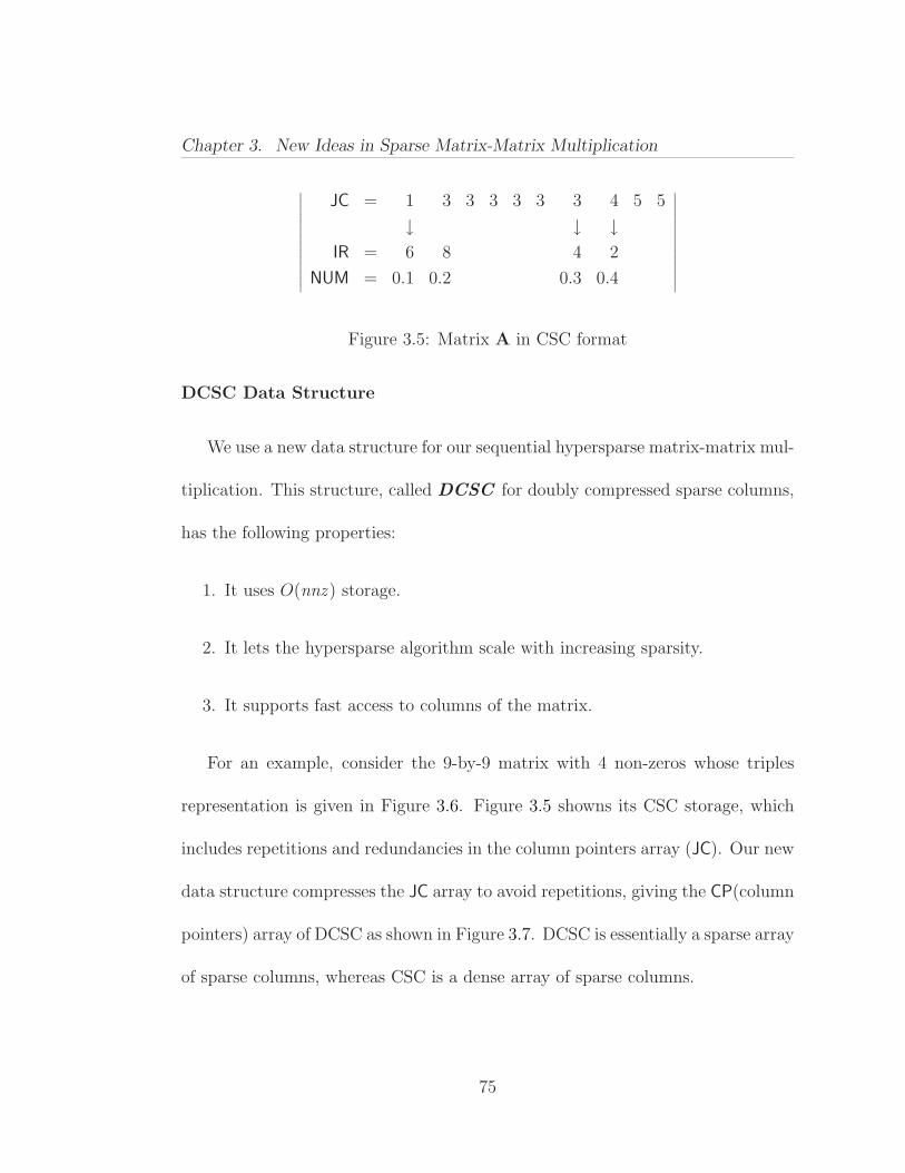
Chapter 3. New Ideas in Sparse Matrix-Matrix Multiplication
˛
˛
˛
˛
˛
˛
˛
˛
˛
˛
˛
˛
˛
˛
JC = 1 3 3 3 3 3 3 4 5 5
↓ ↓ ↓IR = 6 8 4 2
NUM = 0.1 0.2 0.3 0.4
˛
˛
˛
˛
˛
˛
˛
˛
˛
˛
˛
˛
˛
˛
Figure 3.5: Matrix A in CSC format
DCSC Data Structure
We use a new data structure for our sequential hypersparse matrix-matrix mul-
tiplication. This structure, called DCSC for doubly compressed sparse columns,
has the following properties:
1. It uses O(nnz ) storage.
2. It lets the hypersparse algorithm scale with increasing sparsity.
3. It supports fast access to columns of the matrix.
For an example, consider the 9-by-9 matrix with 4 non-zeros whose triples
representation is given in Figure 3.6. Figure 3.5 showns its CSC storage, which
includes repetitions and redundancies in the column pointers array (JC). Our new
data structure compresses the JC array to avoid repetitions, giving the CP(column
pointers) array of DCSC as shown in Figure 3.7. DCSC is essentially a sparse array
of sparse columns, whereas CSC is a dense array of sparse columns.
75

Chapter 3. New Ideas in Sparse Matrix-Matrix Multiplication
! " #$"
% " #$&
' ( #$)
& % #$'
!$* !$+ !$,
Figure 3.6: Matrix A in Triples format
NUM = 0.1 0.2 0.3 0.4
IR = 6 8 4 2
CP = 1 3 4 5
JC = 1 7 8
AUX = 1 2 4 4
Figure 3.7: Matrix A in DCSC format
After removing repetitions, CP[i] does no longer refer to the ith column. A
new JC array, which is parallel to CP, gives us the column numbers. Although
our Hypersparse GEMM algorithm does not need column indexing, DCSC
supports fast column indexing for completeness. Whenever column indexing is
needed, we construct an AUX array that contains pointers to nonzero columns
(columns that have at least one nonzero element). Each entry in AUX refers to
a ⌈n/ nzc⌉-sized chunk of columns, pointing to the first nonzero column in that
chunk (there might be none). The storage requirement of DCSC is O(nnz ) since
|NUM| = |IR| = nnz , |JC| = nzc, |CP| = nzc +1, and |AUX| ≈ nzc.
In our implementation, the AUX array is a temporary work array that is con-
tructed on demand, only when an operation requires repetitive use of it. This
76
Chapter 3. New Ideas in Sparse Matrix-Matrix Multiplication
keeps the storage and copying costs low. The time to construct AUX is only
O(nzc), which is subsumed by the cost of multiplication.
The careful reader will see that DCSC (without the AUX array) resembles two
other data structures. One is the column-major ordered triples representation
from Chapter 2, except we pack all the indices with the same column index into
a single value JC[i], at the cost of introducing a integer pointer CP[i]. DCSC
is also similar in spirit to 2D search trees [99], because we can perform column
indexing using retrieval by primary key, and nonzero indexing within a column
using retrieval by secondary key. This similarity suggests different implementa-
tions of DCSC, including lexicographical splay trees [185] and k-d trees [29]. Our
particular representation is more cache-friendly than conventional 2D search trees
because it uses arrays instead of pointers.
A Sequential Algorithm to Multiply Hypersparse Matrices
The sequential hypersparse algorithm (Hypersparse GEMM) is based on
outer product multiplication. Therefore, it requires fast access to rows of matrix
B. This could be accomplished by having each input matrix represented in DCSC
and also in DCSR (doubly compressed sparse rows), which is the same as the
transpose in DCSC. This method, which we described in an early version of this
work [49], doubles the storage but does not change the asymptotic space and time
77
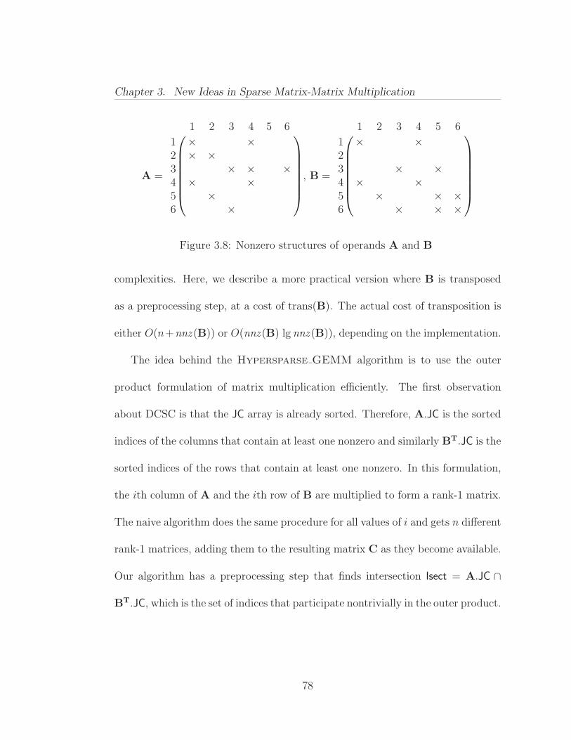
Chapter 3. New Ideas in Sparse Matrix-Matrix Multiplication
A =
1 2 3 4 5 6
1 × ×2 × ×3 × × ×4 × ×5 ×6 ×
, B =
1 2 3 4 5 6
1 × ×23 × ×4 × ×5 × × ×6 × × ×
Figure 3.8: Nonzero structures of operands A and B
complexities. Here, we describe a more practical version where B is transposed
as a preprocessing step, at a cost of trans(B). The actual cost of transposition is
either O(n+nnz (B)) or O(nnz (B) lg nnz (B)), depending on the implementation.
The idea behind the Hypersparse GEMM algorithm is to use the outer
product formulation of matrix multiplication efficiently. The first observation
about DCSC is that the JC array is already sorted. Therefore, A.JC is the sorted
indices of the columns that contain at least one nonzero and similarly BT.JC is the
sorted indices of the rows that contain at least one nonzero. In this formulation,
the ith column of A and the ith row of B are multiplied to form a rank-1 matrix.
The naive algorithm does the same procedure for all values of i and gets n different
rank-1 matrices, adding them to the resulting matrix C as they become available.
Our algorithm has a preprocessing step that finds intersection Isect = A.JC ∩
BT.JC, which is the set of indices that participate nontrivially in the outer product.
78

Chapter 3. New Ideas in Sparse Matrix-Matrix Multiplication
! " # "
! # $ "% !
&'()
*+!,-./ *+$,-./ *+%,-.
&+-,!. &+-,". &+-,$.
#*0'()
% $ 1 #$! $
&+-,1.&+-,#.
% %$1
*+#,-.
1
*+1,-.
!"#"$
!%#"$
!&#"$
!"#&$
!"#$%&
!'#'$
!(#'$
!'#)$
!(#)$
!"#$%'
!"#"$
!'#"$
!&#"$
!"#&$
!"#$%(
!'#'$
!'#)$
!'#($
!"#$%)
!%#&$
!&#&$
!'#&$
!&#&$
Figure 3.9: Cartesian product and the multiway merging analogy
The preprocessing takes O(nzc(A) + nzr(B)) time as |A.JC| = nzc(A) and
|BT.JC| = nzr(B). The next phase of our algorithm performs |Isect| cartesian
products, each of which generates a fictitious list of size nnz (A(:, i)) ·nnz (B(i, :)).
The lists can be generated sorted, because all the elements within a given column
are sorted according to their row indices (i.e. IR(JC(i))...IR(JC(i) + 1) is a sorted
range). The algorithm merges those sorted lists, summing up the intermediate
entries having the same (row id, col id) index pair, to form the resulting matrix
C. Therefore, the second phase of Hypersparse GEMM is similar to multiway
merging [128]. The only difference is that we never explicitly construct the lists;
we compute their elements one-by-one on demand.
Figure 3.9 shows the setup for the matrices from Figure 3.8. As A.JC =
1, 2, 3, 4, 6 and BT.JC = 1, 3, 4, 5, 6, Isect = 1, 3, 4, 6 for this product. The
algorithm does not touch the shaded elements, since they do not contribute to the
output.
79
Chapter 3. New Ideas in Sparse Matrix-Matrix Multiplication
The merge uses a priority queue (represented as a heap) of size ni , which is
the size of Isect, the number of indices i for which A(:, i) 6= ∅ and B(i, :) 6= ∅. The
value in a heap entry is its NUM value and the key is a pair of indices (i, j) in
column-major order. The idea is to repeatedly extract the entry with minimum
key from the heap and insert another element from the list that the extracted
element originally came from. If there are multiple elements in the lists with the
same key, then their values are added on the fly. If we were to explicitly create
ni lists instead of doing the computation on the fly, we would get the lists shown
in the right side of Figure 3.9, which are sorted from bottom to top. For further
details of multiway merging, consult Knuth [128].
The time complexity of this phase is O(flops · lg ni), and the space complexity
is O(nnz (C) + ni). The output is a stack of NUM values in column-major order.
The nnz (C) term in the space complexity comes from the output, and the flops
term in the time complexity comes from the observation that
∑
i∈Isect
nnz (A(:, i)) · nnz (B(i, :)) = flops.
The final phase of the algorithm constructs the DCSC structure from this
column-major-ordered stack. This requires O(nnz (C)) time and space.
The overall time complexity of our algorithm is O(nzc(A) + nzr(B) + flops ·
lg ni), plus the preprocessing time to transpose matrix B. Note that nnz (C)
does not appear in this bound, since nnz (C) ≤ flops. We opt to keep the cost
80
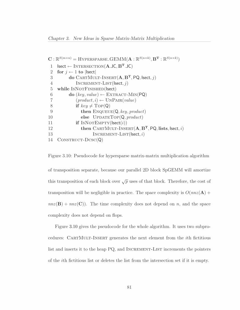
Chapter 3. New Ideas in Sparse Matrix-Matrix Multiplication
C : RS(m×n) = Hypersparse GEMM(A : R
S(n×k),BT : RS(n×k))
1 Isect← Intersection(A.JC,BT.JC)2 for j ← 1 to |Isect|3 do CartMult-Insert(A,BT, PQ, Isect, j)4 Increment-List(Isect, j)5 while IsNotFinished(Isect)6 do (key , value)← Extract-Min(PQ)7 (product , i)← UnPair(value)8 if key 6= Top(Q)9 then Enqueue(Q, key , product)
10 else UpdateTop(Q, product)11 if IsNotEmpty(Isect(i))12 then CartMult-Insert(A,BT, PQ, lists, Isect, i)13 Increment-List(Isect, i)14 Construct-Dcsc(Q)
Figure 3.10: Pseudocode for hypersparse matrix-matrix multiplication algorithm
of transposition separate, because our parallel 2D block SpGEMM will amortize
this transposition of each block over√
p uses of that block. Therefore, the cost of
transposition will be negligible in practice. The space complexity is O(nnz (A) +
nnz (B) + nnz (C)). The time complexity does not depend on n, and the space
complexity does not depend on flops.
Figure 3.10 gives the pseudocode for the whole algorithm. It uses two subpro-
cedures: CartMult-Insert generates the next element from the ith fictitious
list and inserts it to the heap PQ, and Increment-List increments the pointers
of the ith fictitious list or deletes the list from the intersection set if it is empty.
81

Chapter 3. New Ideas in Sparse Matrix-Matrix Multiplication
To justify the extra logarithmic factor in the flops term, we briefly analyze the
complexity of each submatrix multiplication in the parallel 2D block SpGEMM.
Our parallel 2D block SpGEMM performs p√
p submatrix multiplications, since
each submatrix of the output is computed using Cij =∑√
p
k=1 Aik Bkj. Therefore,
with increasing number of processors and under perfect load balance, flops scale
with 1/p√
p, nnz scale with 1/p, and n scales with 1/√
p. Figure 3.11 shows
the trends of these three complexity measures as p increases. The graph shows
that the n term becomes the bottleneck after around 50 processors and flops
becomes the lower-order term. In contrast to the classical algorithm, our Hyper-
sparse GEMM algorithm becomes independent of n, by putting the burden on
the flops instead.
3.2.2 Sparse Matrices with Large Dimension
Even for ordinary large sparse matrices (nnz = O(n)), the use of SPA in the
classical algorithm can hurt the performance. As shown in the previous chapter,
the classical algorithm has an I/O complexity of O(scan(A) + flops), because the
fast memory (cache) is often not big enough to hold a O(n) data structure like
SPA. In this section, we give a cache-friendly formulation of the column-by-column
algorithm that uses a heap instead of a SPA.
82
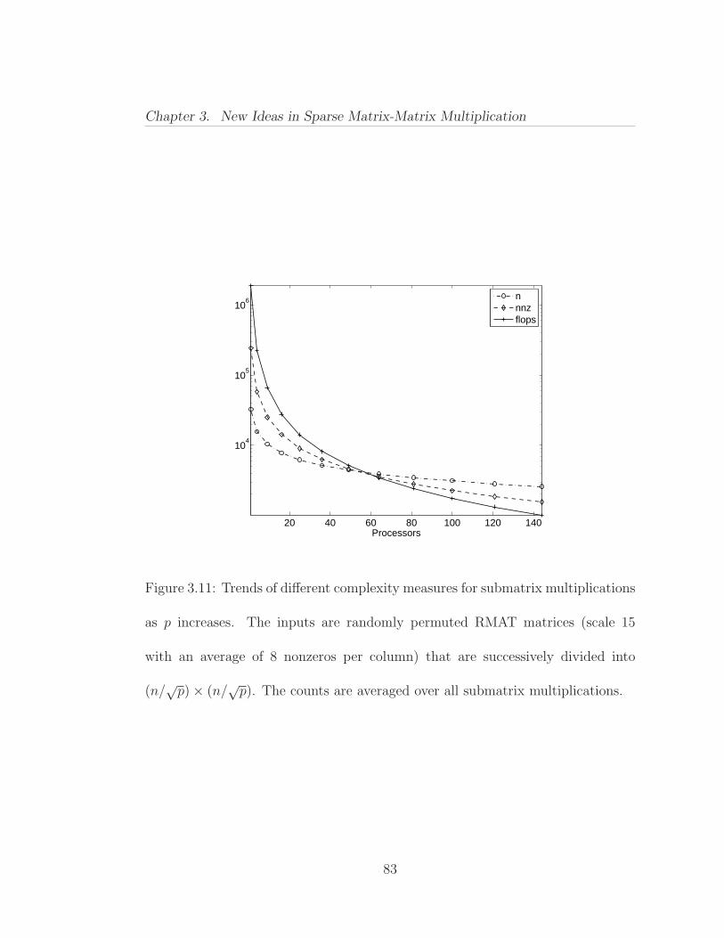
Chapter 3. New Ideas in Sparse Matrix-Matrix Multiplication
20 40 60 80 100 120 140
104
105
106
Processors
nnnzflops
Figure 3.11: Trends of different complexity measures for submatrix multiplications
as p increases. The inputs are randomly permuted RMAT matrices (scale 15
with an average of 8 nonzeros per column) that are successively divided into
(n/√
p)× (n/√
p). The counts are averaged over all submatrix multiplications.
83
Chapter 3. New Ideas in Sparse Matrix-Matrix Multiplication
A Cache Efficient Sequential Algorithm
Our second algorithm is based on the column-by-column formulation the classi-
cal algorithm. Any data structure that can enumerate nonzeros in the jth column
in O(nnz (j)) time is suitable for this algorithm, so we assume that the matrices
are in CSC format for simplicity. Equivalently, we could have used DCSC to avoid
any format conversion in case this subroutine is used as part of a polyalgorithm.
Similar to the classical algorithm, we will be computing a whole column of C in
one step by examining the same column of B. In other words, C(:, j) is a lin-
ear combination of the columns A(:, i) for which B(i, j) 6= 0. Time complexity,
however, is independent of m since we do not use a SPA.
For the construction of C(:, j), we use a heap of size nnz (B(:, j)). As in the
case of the hypersparse algorithm, we require the row indices within each column
to be sorted. The idea of merging columns using a heap has been employed
before, within the Ordered-SPA data structure [124]. However, the Ordered-SPA
was never used to suppress the m factor in the algorithm because it is an Θ(m)
data structure. Furthermore, the Ordered-SPA uses a heap of size nnz (C(:, j)),
which can be much bigger than nnz (B(:, j)).
Figure 3.12 illustrates the algorithm where column j of C is computed as a
linear combination of the columns of A as specified by the nonzeros in column j
84
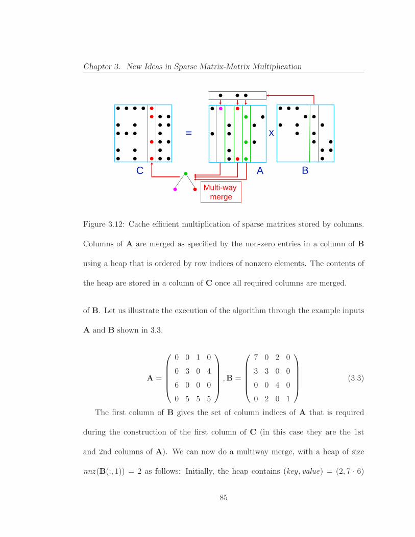
Chapter 3. New Ideas in Sparse Matrix-Matrix Multiplication
B
= x
C A
Multi-way merge
Figure 3.12: Cache efficient multiplication of sparse matrices stored by columns.
Columns of A are merged as specified by the non-zero entries in a column of B
using a heap that is ordered by row indices of nonzero elements. The contents of
the heap are stored in a column of C once all required columns are merged.
of B. Let us illustrate the execution of the algorithm through the example inputs
A and B shown in 3.3.
A =
0 0 1 0
0 3 0 4
6 0 0 0
0 5 5 5
,B =
7 0 2 0
3 3 0 0
0 0 4 0
0 2 0 1
(3.3)
The first column of B gives the set of column indices of A that is required
during the construction of the first column of C (in this case they are the 1st
and 2nd columns of A). We can now do a multiway merge, with a heap of size
nnz (B(:, 1)) = 2 as follows: Initially, the heap contains (key , value) = (2, 7 · 6)
85
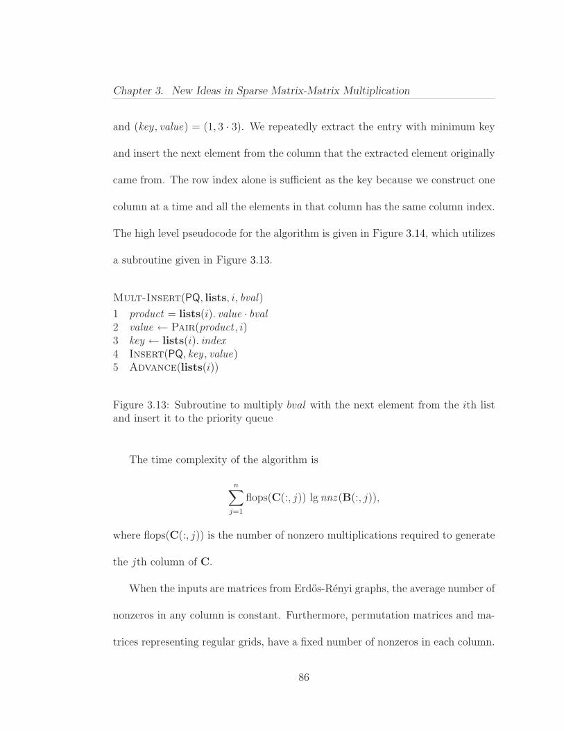
Chapter 3. New Ideas in Sparse Matrix-Matrix Multiplication
and (key , value) = (1, 3 · 3). We repeatedly extract the entry with minimum key
and insert the next element from the column that the extracted element originally
came from. The row index alone is sufficient as the key because we construct one
column at a time and all the elements in that column has the same column index.
The high level pseudocode for the algorithm is given in Figure 3.14, which utilizes
a subroutine given in Figure 3.13.
Mult-Insert(PQ, lists, i, bval)
1 product = lists(i). value · bval2 value ← Pair(product , i)3 key ← lists(i). index4 Insert(PQ, key , value)5 Advance(lists(i))
Figure 3.13: Subroutine to multiply bval with the next element from the ith listand insert it to the priority queue
The time complexity of the algorithm is
n∑
j=1
flops(C(:, j)) lg nnz (B(:, j)),
where flops(C(:, j)) is the number of nonzero multiplications required to generate
the jth column of C.
When the inputs are matrices from Erdos-Renyi graphs, the average number of
nonzeros in any column is constant. Furthermore, permutation matrices and ma-
trices representing regular grids, have a fixed number of nonzeros in each column.
86
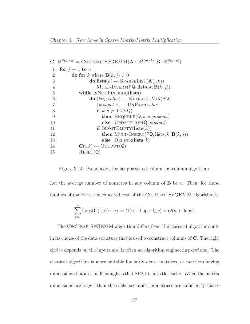
Chapter 3. New Ideas in Sparse Matrix-Matrix Multiplication
C : RS(m×n) = CscHeap SpGEMM(A : R
S(m×k),B : RS(k×n))
1 for j ← 1 to n2 do for k where B(k, j) 6= 03 do lists(k)← SparseList(A(:, k))4 Mult-Insert(PQ, lists, k,B(k, j))5 while IsNotFinished(lists)6 do (key , value)← Extract-Min(PQ)7 (product , i)← UnPair(value)8 if key 6= Top(Q)9 then Enqueue(Q, key , product)
10 else UpdateTop(Q, product)11 if IsNotEmpty(lists(k))12 then Mult-Insert(PQ, lists, k,B(k, j))13 else Delete(lists, k)14 C(:, k)← Output(Q)15 Reset(Q)
Figure 3.14: Pseudocode for heap assisted column-by-column algorithm
Let the average number of nonzeros in any column of B be c. Then, for those
families of matrices, the expected cost of the CscHeap SpGEMM algorithm is
n∑
j=1
flops(C(:, j)) · lg c = O(n + flops · lg c) = O(n + flops).
The CscHeap SpGEMM algorithm differs from the classical algorithm only
in its choice of the data structure that is used to construct columns of C. The right
choice depends on the inputs and is often an algorithm engineering decision. The
classical algorithm is more suitable for fairly dense matrices, or matrices having
dimensions that are small enough so that SPA fits into the cache. When the matrix
dimensions are bigger than the cache size and the matrices are sufficiently sparse
87
Chapter 3. New Ideas in Sparse Matrix-Matrix Multiplication
so that the added lg c factor is negligible, we expect CscHeap SpGEMM to
outperform the classical algorithm. We verify our intuition through experiments
in Section 3.2.3.
3.2.3 Performance of the Cache Efficient Algorithm
In order to unveil the effects of cache misses on the column-by-column SpGEMM
algorithms, we ran experiments with matrix dimensions varying from 103 to 106.
For matrix dimension, we timed the multiplication of two sparse matrices from
Erdos-Renyi graphs with average nonzeros per column varying from 2 to 32.
Our test platform is a 2.2 Ghz Opteron that has 512 KB L2 cache per core.
Therefore, SPA starts to fall out of L2 cache around n = 105. We compared two
column-wise algorithms: the classical algorithm that uses a SPA and the cache-
friendly algorithm explained in Section 3.2.2 that uses a heap. We implemented
both algorithms using C++ and compiled them with the Intel C++ compiler ver-
sion 9.1, as it is the best performing compiler on our system, with the optimization
flag -fast .
The results for n = 104 show the case where SPA completely fits into the
cache. In this case, as shown in Figure 3.15(a), both algorithms are comparable
in terms of performance, with only a marginal difference of at most ±5%. On the
other hand, Figure 3.15(a) shows the results for 106 where SPA falls out of cache.
88

Chapter 3. New Ideas in Sparse Matrix-Matrix Multiplication
The advantage of using a heap is more pronounced in this case, with relative
performance increases varying from 24% to 55% over the SPA based version.
2.56
0.64
0.16
0.04
0.01
32 16 8 4 2
Tim
e (s
ecs)
Average nonzeros per column
Heap MergeSPA Merge
(a) n = 104
512
128
32
8
2
32 16 8 4 2
Tim
e (s
ecs)
Average nonzeros per column
Heap MergeSPA Merge
(b) n = 106
Figure 3.15: Performance of two column-wise algorithms for multiplying two n×n
sparse matrices from Erdos-Renyi random graphs
89
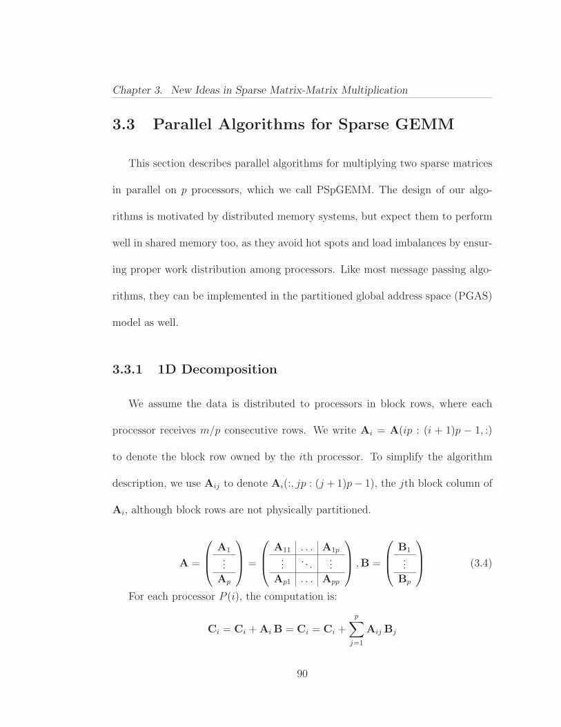
Chapter 3. New Ideas in Sparse Matrix-Matrix Multiplication
3.3 Parallel Algorithms for Sparse GEMM
This section describes parallel algorithms for multiplying two sparse matrices
in parallel on p processors, which we call PSpGEMM. The design of our algo-
rithms is motivated by distributed memory systems, but expect them to perform
well in shared memory too, as they avoid hot spots and load imbalances by ensur-
ing proper work distribution among processors. Like most message passing algo-
rithms, they can be implemented in the partitioned global address space (PGAS)
model as well.
3.3.1 1D Decomposition
We assume the data is distributed to processors in block rows, where each
processor receives m/p consecutive rows. We write Ai = A(ip : (i + 1)p − 1, :)
to denote the block row owned by the ith processor. To simplify the algorithm
description, we use Aij to denote Ai(:, jp : (j + 1)p− 1), the jth block column of
Ai, although block rows are not physically partitioned.
A =
A1
...Ap
=
A11 . . . A1p
.... . .
...Ap1 . . . App
,B =
B1
...Bp
(3.4)
For each processor P (i), the computation is:
Ci = Ci + Ai B = Ci = Ci +
p∑
j=1
Aij Bj
90
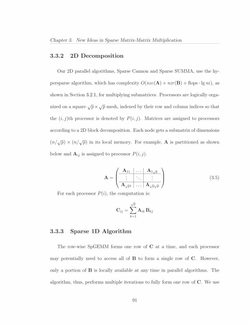
Chapter 3. New Ideas in Sparse Matrix-Matrix Multiplication
3.3.2 2D Decomposition
Our 2D parallel algorithms, Sparse Cannon and Sparse SUMMA, use the hy-
persparse algorithm, which has complexity O(nzc(A) + nzr(B) + flops · lg ni), as
shown in Section 3.2.1, for multiplying submatrices. Processors are logically orga-
nized on a square√
p×√p mesh, indexed by their row and column indices so that
the (i, j)th processor is denoted by P (i, j). Matrices are assigned to processors
according to a 2D block decomposition. Each node gets a submatrix of dimensions
(n/√
p) × (n/√
p) in its local memory. For example, A is partitioned as shown
below and Aij is assigned to processor P (i, j).
A =
A11 . . . A1√
p
.... . .
...A√
p1 . . . A√p√
p
(3.5)
For each processor P (i), the computation is:
Cij =
√p∑
k=1
Aik Bkj
3.3.3 Sparse 1D Algorithm
The row-wise SpGEMM forms one row of C at a time, and each processor
may potentially need to access all of B to form a single row of C. However,
only a portion of B is locally available at any time in parallel algorithms. The
algorithm, thus, performs multiple iterations to fully form one row of C. We use
91
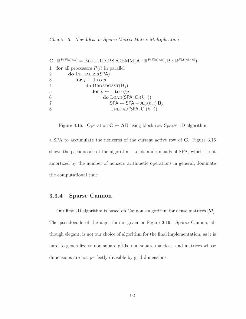
Chapter 3. New Ideas in Sparse Matrix-Matrix Multiplication
C : RP (S(n)×n) = Block1D PSpGEMM(A : R
P (S(n)×n),B : RP (S(n)×n))
1 for all processors P (i) in parallel2 do Initialize(SPA)3 for j ← 1 to p4 do Broadcast(Bj)5 for k ← 1 to n/p6 do Load(SPA,Ci(k, :))7 SPA← SPA + Aij(k, :)Bj
8 Unload(SPA,Ci(k, :))
Figure 3.16: Operation C← AB using block row Sparse 1D algorithm
a SPA to accumulate the nonzeros of the current active row of C. Figure 3.16
shows the pseudocode of the algorithm. Loads and unloads of SPA, which is not
amortized by the number of nonzero arithmetic operations in general, dominate
the computational time.
3.3.4 Sparse Cannon
Our first 2D algorithm is based on Cannon’s algorithm for dense matrices [52].
The pseudocode of the algorithm is given in Figure 3.19. Sparse Cannon, al-
though elegant, is not our choice of algorithm for the final implementation, as it is
hard to generalize to non-square grids, non-square matrices, and matrices whose
dimensions are not perfectly divisible by grid dimensions.
92
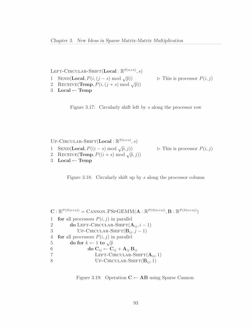
Chapter 3. New Ideas in Sparse Matrix-Matrix Multiplication
Left-Circular-Shift(Local : RS(n×n), s)
1 Send(Local, P (i, (j − s) mod√
p)) This is processor P (i, j)2 Receive(Temp, P (i, (j + s) mod
√p))
3 Local← Temp
Figure 3.17: Circularly shift left by s along the processor row
Up-Circular-Shift(Local : RS(n×n), s)
1 Send(Local, P ((i− s) mod√
p, j)) This is processor P (i, j)2 Receive(Temp, P ((i + s) mod
√p, j))
3 Local← Temp
Figure 3.18: Circularly shift up by s along the processor column
C : RP (S(n×n)) = Cannon PSpGEMM(A : R
P (S(n×n)),B : RP (S(n×n)))
1 for all processors P (i, j) in parallel2 do Left-Circular-Shift(Aij, i− 1)3 Up-Circular-Shift(Bij, j − 1)4 for all processors P (i, j) in parallel5 do for k ← 1 to
√p
6 do Cij ← Cij + Aij Bij
7 Left-Circular-Shift(Aij, 1)8 Up-Circular-Shift(Bij, 1)
Figure 3.19: Operation C← AB using Sparse Cannon
93
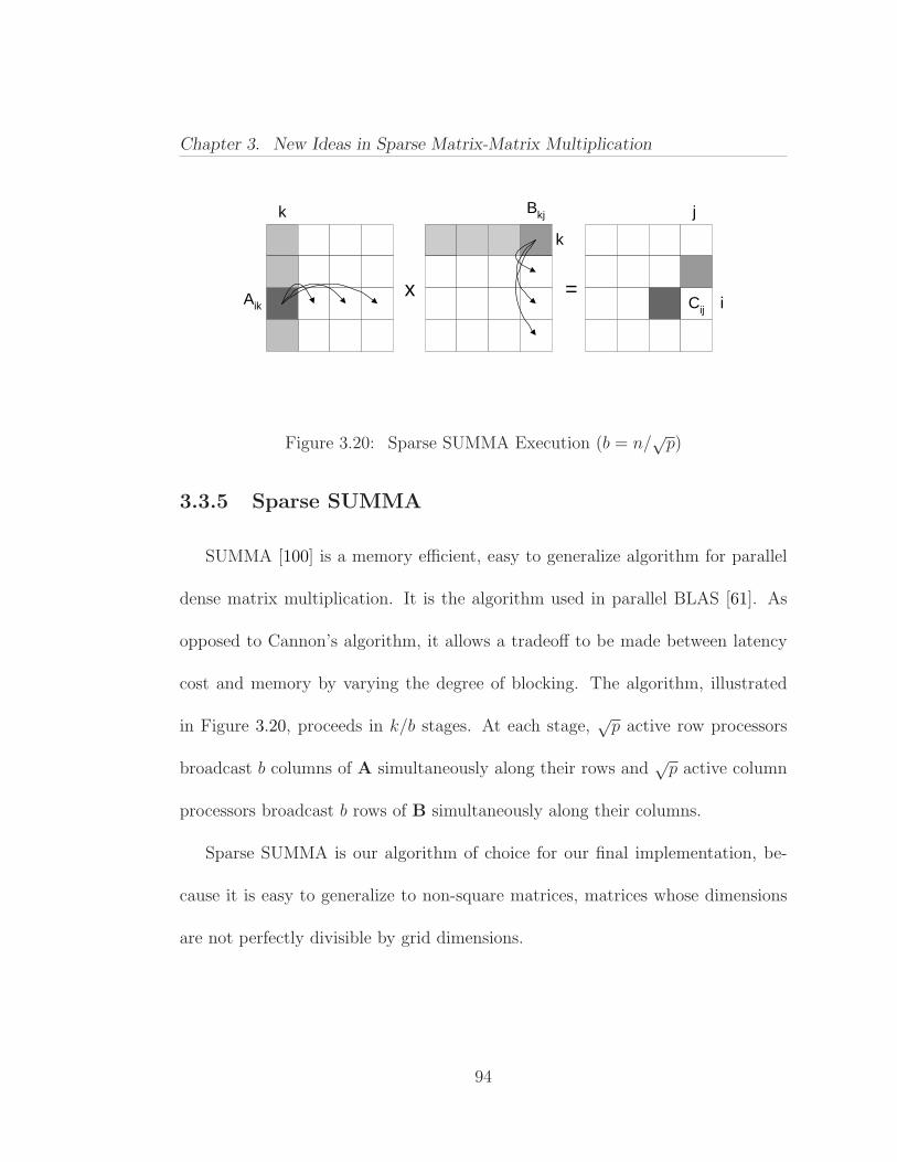
Chapter 3. New Ideas in Sparse Matrix-Matrix Multiplication
Cij
x =Aik
Bkjk
k
j
i
Figure 3.20: Sparse SUMMA Execution (b = n/√
p)
3.3.5 Sparse SUMMA
SUMMA [100] is a memory efficient, easy to generalize algorithm for parallel
dense matrix multiplication. It is the algorithm used in parallel BLAS [61]. As
opposed to Cannon’s algorithm, it allows a tradeoff to be made between latency
cost and memory by varying the degree of blocking. The algorithm, illustrated
in Figure 3.20, proceeds in k/b stages. At each stage,√
p active row processors
broadcast b columns of A simultaneously along their rows and√
p active column
processors broadcast b rows of B simultaneously along their columns.
Sparse SUMMA is our algorithm of choice for our final implementation, be-
cause it is easy to generalize to non-square matrices, matrices whose dimensions
are not perfectly divisible by grid dimensions.
94
Chapter 3. New Ideas in Sparse Matrix-Matrix Multiplication
3.4 Analysis of Parallel Algorithms
In this section, we analyze the parallel performance of our algorithms, and
show that they scale better than existing 1D algorithms in theory. We begin
by introducing our parameters and model of computation. Then, we present a
theoretical analysis showing that 1D decomposition, at least with the current
algorithm, is not sufficient for PSpGEMM to scale. Finally, we analyze our 2D
algorithms in depth.
In our analysis, the cost of one floating-point operation, along with the cost
of cache misses and memory indirections associated with the operation, is de-
noted by γ, measured in nanoseconds. The latency of sending a message over
the communication interconnect is α, and the inverse bandwidth is β, measured
in nanoseconds and nanoseconds per word transfered, respectively. The running
time of a parallel algorithm on p processors is given by
Tp = Tcomm + Tcomp,
where Tcomm denotes the time spent in communication and Tcomp is the time spent
during local computation phases. Tcomm includes both the latency (delay) costs
and the actual time it takes to transfer the data words over the network. Hence,
the cost of transmitting h data words in a communication phase is
Tcomm = α + hβ.
95
Chapter 3. New Ideas in Sparse Matrix-Matrix Multiplication
The sequential work of SpGEMM, unlike dense GEMM, depends on many
parameters. This makes parallel scalability analysis a tough process. Therefore,
we restrict our analysis to sparse matrices following the Erdos-Renyi graph model
explained in Section 1.5.2. Consequently, the analysis is probabilistic, exploiting
the independent and identical distribution of nonzeros. When we talk about
quantities such as nonzeros per subcolumn, we mean the expected number of
nonzeros. Our analysis assumes that there are c > 0 nonzeros per row/column.
The sparsity parameter c, albeit oversimplifying, is useful for analysis purposes,
since it makes different parameters comparable to each other. For example, if A
and B both have sparsity c, then nnz (A) = cn and flops(AB) = c2n. It also
allows us to decouple the effects of load imbalances from the algorithm analysis
because the nonzeros are assumed to be evenly distributed across processors.
The lower bound on sequential SpGEMM is Ω(flops) = Ω(c2n). This bound is
achieved by some row-wise and column-wise implementations [104, 113], provided
that c ≥ 1. The row-wise implementation of Gustavson that uses CSR is the
natural kernel to be used in the 1D algorithm where data is distributed by rows.
As shown in the previous chapter, it has an asymptotic complexity of
O(n + nnz (A) + flops) = O(n + cn + c2n) = Θ(c2n).
Therefore, we take the sequential work (W ) to be γc2n in our analysis.
96
Chapter 3. New Ideas in Sparse Matrix-Matrix Multiplication
3.4.1 Scalability of the 1D Algorithm
We begin with a theoretical analysis whose conclusion is that 1D decomposition
is not sufficient for PSpGEMM to scale. In Block1D PSpGEMM, each proces-
sor sends and receives p− 1 point-to-point messages of size nnz (B)/p. Therefore,
Tcomm = (p− 1)(α + β
nnz (B)
p
)= Θ(p α + β c n). (3.6)
We previously showed that the Block1D PSpGEMM algorithm is unscal-
able with respect to both communication and computation costs [48]. In fact, it
gets slower as the number of processors grow. The current Star-P implemen-
tation [180] by-passes this problem by all-to-all broadcasting nonzeros of the B
matrix, so that the whole B matrix is essentially assembled at each processor.
This avoids the cost of loading and unloading SPA at every stage, but it uses
nnz (B) memory at each processor.
3.4.2 Scalability of the 2D Algorithms
In this section, we provide an in-depth theoretical analysis of our parallel 2D
SpGEMM algorithms, and conclude that they scale significantly better than their
1D counterparts. Although our analysis is limited to the Erdos-Renyi model, its
conclusions are strong enough to be convincing.
97
Chapter 3. New Ideas in Sparse Matrix-Matrix Multiplication
In Cannon PSpGEMM, each processor sends and receives√
p− 1 point-to-
point messages of size nnz (A)/p, and√
p−1 messages of size nnz (B)/p. Therefore,
the communication cost per processor is
Tcomm =√
p(2 α + β
(nnz (A) + nnz (B)
p
))= Θ(α
√p +
β c n√p
). (3.7)
The average number of nonzeros in a column of a local submatrix Aij is c/√
p.
Therefore, for a submatrix multiplication AikBkj,
ni(Aik,Bkj) = min1,
c2
p
n√p
= min n√p,c2 n
p√
p,
flops(AikBkj) =flops(AB)
p√
p=
c2 n
p√
p,
Tmult =√
p
(2 min
1,
c√p
n√p
+c2n
p√
plg
(min
n√p,
c2n
p√
p
)).
The probability of a single column of Aik (or a single row of Bkj) having at
least one nonzero is min1, c/√p where 1 covers the case p ≤ c2 and c/√
p covers
the case p > c2.
The overall cost of additions, using p processors, and Brown and Tarjan’s
O(m lg n/m) algorithm [46] for merging two sorted lists of size m and n (for
m < n), is
98
Chapter 3. New Ideas in Sparse Matrix-Matrix Multiplication
Tadd =
√p∑
i=1
(flops
p√
plg i
)=
flops
p√
plg
√p∏
i=1
i =flops
p√
plg (√
p !).
Note that we might be slightly overestimating, since we assume flops/ nnz (C) ≈
1 for simplicity. From Stirling’s approximation and asymptotic analysis, we know
that lg (n !) = Θ(n lg n) [68]. Thus, we get:
Tadd = Θ(flops
p√
p
√p lg√
p
)= Θ
(c2n lg
√p
p
).
There are two cases to analyze: p > c2 and p ≤ c2. Since scalability analysis
is concerned with the asymptotic behavior as p increases, we just provide results
for the p > c2 case. The total computation cost Tcomp = Tmult + Tadd is
Tcomp = γ( c n√
p+
c2n
plg
( c2n
p√
p
)+
c2n lg√
p
p
)= γ
( c n√p
+c2n
plg
(c2n
p
)). (3.8)
In this case, parallel efficiency is
E =W
p(Tcomp + Tcomm
) =γc2n
(γ + β) c n√
p + γc2n lg(
c2np
)+ α p
√p. (3.9)
Scalability is not perfect and efficiency deteriorates as p increases due to the
first term. Speedup is, however, not bounded, as opposed to the 1D case. In par-
ticular, lg (c2n/p) becomes negligible as p increases and scalability due to latency
is achieved when γc2n ∝ α p√
p, where it is sufficient for n to grow on the order
of p1.5. The biggest bottleneck for scalability is the first term in the denominator,
99
Chapter 3. New Ideas in Sparse Matrix-Matrix Multiplication
which scales with√
p. Consequently, two different scaling regimes are likely to be
present: A close to linear scaling regime until the first term starts to dominate
the denominator and a√
p-scaling regime afterwards.
Compared to the 1D algorithms, Sparse Cannon both lower the degree of
unscalability due to bandwidth costs and mitigate the bottleneck of computation.
This makes overlapping communication with computation more promising.
Sparse SUMMA, like dense SUMMA, incurs an extra cost over Cannon for us-
ing row-wise and col-wise broadcasts instead of nearest-neighbor communication,
which might be modeled as an additional O(lg p) factor in communication cost.
Other than that, the analysis is similar to sparse Cannon and we omit the de-
tails. Using the DCSC data structure, the expected cost of fetching b consecutive
columns of a matrix A is b plus the size (number of nonzeros) of the output [49].
Therefore, the algorithm asymptotically has the same computation cost for all
values of b.
3.5 Performance Modeling of Parallel Algorithms
In this section, we first project the estimated speedup of 1D and 2D algo-
rithms in order to evaluate their prospects in practice. We use a quasi-analytical
performance model where we first obtain realistic values for the parameters (γ,
100
Chapter 3. New Ideas in Sparse Matrix-Matrix Multiplication
β, α) of the algorithm performance, then use them in our projections. In the sec-
ond part, we perform another modeling study where we simulate the execution of
Sparse SUMMA using an actual implementation of the Hypersparse GEMM
algorithm. This modeling study concludes that Hypersparse GEMM is scal-
able with increasing hypersparsity, suggesting that it is a suitable algorithm to be
the sequential kernel of a 2D parallel SpGEMM.
3.5.1 Estimated Speedup of Parallel Algorithms
This study estimates the speedup of 1D and 2D algorithms by using a quasi-
analytic model that projects the performance on large systems using realistic
values for the performance parameters.
In order to obtain a realistic value for γ, we performed multiple runs on an
AMD Opteron 8214 (Santa Rosa) processor using matrices of various dimensions
and sparsity; estimating the constants using non-linear regression. One surprising
result is the order of magnitude difference in the constants between sequential
kernels. The classical algorithm, which is used as the 1D SpGEMM kernel, has
γ = 293.6 nsec, whereas Hypersparse GEMM, which is used as the 2D ker-
nel, has γ = 19.2 nsec. We attribute the difference to cache friendliness of the
hypersparse algorithm. The interconnect supports β = 1 GB/sec point-to-point
bandwidth, and a maximum of α = 2.3 microseconds latency, both of which are
101

Chapter 3. New Ideas in Sparse Matrix-Matrix Multiplication
achievable on TACC’s Ranger Cluster. The communication parameters ignore
network contention.
01000
20003000
40005000
0
0.5
1
1.5
2
x 107
0
5
10
15
20
25
30
35
40
45
Num ProcsMatrix Dimension N
Figure 3.21: Modeled speedup of Synchronous Sparse 1D algorithm
Figures 3.21 and 3.22 show the modeled speedup of Block1D PSpGEMM
and Cannon PSpGEMM for matrix dimensions from n = 217 to 224 and number
of processors from p = 1 to 4096. The inputs are Erdos-Renyi graphs.
We see that Block1D PSpGEMM’s speedup does not go beyond 50x, even
on larger matrices. For relatively small matrices, having dimensions n = 217−220,
it starts slowing down after a thousand processors, where it achieves less than 40x
speedup. On the other hand, Cannon PSpGEMM shows increasing and almost
linear speedup for up to 4096 processors, even though the slope of the curve is less
102
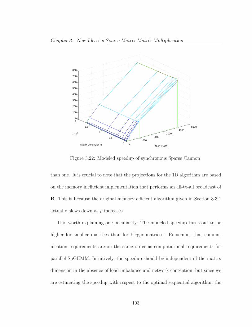
Chapter 3. New Ideas in Sparse Matrix-Matrix Multiplication
01000
20003000
40005000
0
0.5
1
1.5
2
x 107
0
100
200
300
400
500
600
700
800
Num ProcsMatrix Dimension N
Figure 3.22: Modeled speedup of synchronous Sparse Cannon
than one. It is crucial to note that the projections for the 1D algorithm are based
on the memory inefficient implementation that performs an all-to-all broadcast of
B. This is because the original memory efficient algorithm given in Section 3.3.1
actually slows down as p increases.
It is worth explaining one peculiarity. The modeled speedup turns out to be
higher for smaller matrices than for bigger matrices. Remember that commu-
nication requirements are on the same order as computational requirements for
parallel SpGEMM. Intuitively, the speedup should be independent of the matrix
dimension in the absence of load imbalance and network contention, but since we
are estimating the speedup with respect to the optimal sequential algorithm, the
103
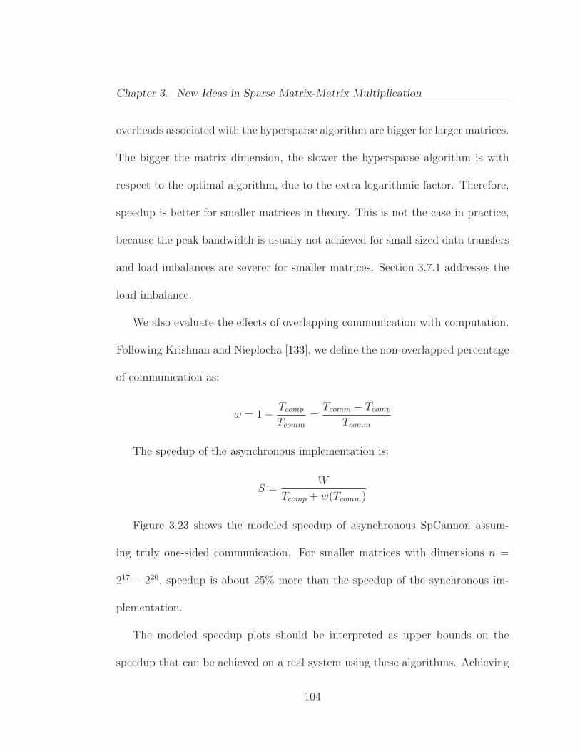
Chapter 3. New Ideas in Sparse Matrix-Matrix Multiplication
overheads associated with the hypersparse algorithm are bigger for larger matrices.
The bigger the matrix dimension, the slower the hypersparse algorithm is with
respect to the optimal algorithm, due to the extra logarithmic factor. Therefore,
speedup is better for smaller matrices in theory. This is not the case in practice,
because the peak bandwidth is usually not achieved for small sized data transfers
and load imbalances are severer for smaller matrices. Section 3.7.1 addresses the
load imbalance.
We also evaluate the effects of overlapping communication with computation.
Following Krishnan and Nieplocha [133], we define the non-overlapped percentage
of communication as:
w = 1− Tcomp
Tcomm
=Tcomm − Tcomp
Tcomm
The speedup of the asynchronous implementation is:
S =W
Tcomp + w(Tcomm)
Figure 3.23 shows the modeled speedup of asynchronous SpCannon assum-
ing truly one-sided communication. For smaller matrices with dimensions n =
217 − 220, speedup is about 25% more than the speedup of the synchronous im-
plementation.
The modeled speedup plots should be interpreted as upper bounds on the
speedup that can be achieved on a real system using these algorithms. Achieving
104

Chapter 3. New Ideas in Sparse Matrix-Matrix Multiplication
01000
20003000
40005000
0
0.5
1
1.5
2
x 107
0
200
400
600
800
1000
1200
Num ProcsMatrix Dimension N
Figure 3.23: Modeled speedup of asynchronous Sparse Cannon
these speedups on real systems requires all components to be implemented and
working optimally. The conclusion we derive from those plots is that no mat-
ter how hard we try, it is impossible to get good speedup with the current 1D
algorithms.
3.5.2 Scalability with Hypersparsity
This modeling study reveals the scalability of our hypersparse algorithm with
increasing sparsity. We have implemented our data structures and multiplica-
tion algorithms in C++. Our code is compiled using the GNU Compiler Col-
lection (GCC) Version 4.1, with the flags -03, because these are the settings
105

Chapter 3. New Ideas in Sparse Matrix-Matrix Multiplication
that our comparison platform, Matlab, is compiled with. We have incorporated
Peter Sander’s Sequence Heaps [174] for all the priority queues used by our al-
gorithms. Througout the experiments, the numerical values are represented as
double-precision floating points.
We compare the performance of our implementation with Matlab R2007A’s
(64-bit version) implementation of the classical algorithm. Sparse matrix multipli-
cation is a built-in function in Matlab, so there are no interpretation overheads
associated with it. We are simply comparing our C++ code with the underlying
precompiled C code used in Matlab.
All of our experiments are performed on a single core of Opteron 2.2 Ghz with
64 GB main memory, where we simulate the execution of a parallel SpGEMM.
The simulation is done by dividing the input matrices of size n×n into p subma-
trices of size (n/√
p)× (n/√
p) using the 2D block decomposition, as explained in
Section 3.3.2 and shown in Figure 3.5.
Expressing the matrix multiplication as algebraic operations on submatrices
instead of individual elements, we see that each submatrix of the product is com-
puted using Cij =∑√
p
k=1 Aik Bkj. Since we are primarily concerned with the
sequential sparse matrix multiplication kernel, we will exclude the cost of subma-
trix additions and other parallel overheads. That is to say, we will only time the
106
Chapter 3. New Ideas in Sparse Matrix-Matrix Multiplication
submatrix multiplications, exactly plotting
time(p,A,B) =
√p∑
i=1
√p∑
j=1
√p∑
k=1
time(Aik Bkj),
which is equal to the amount of work done by a parallel matrix multiplication
algorithm such as SUMMA [100].
Increasing p in this case does not mean we use more processors to compute the
product. Instead, it means we use smaller and smaller blocks while computing
the product on a single processor. Therefore, a perfectly scalable algorithm would
yield flat timing curves as p increases. We expect our hypersparse algorithm
to outperform the classical algorithm as p increases due to reasons explained
in Section 3.2.1. We label the classical algorithm Matlab, and our algorithm
Hypersparse GEMM in the plots. The second input is only transposed once
because this is what would happen in a parallel implementation.
In all experiments in this section, the input matrices have dimensions 223×223,
i.e. the input graphs have around 8 million vertices.
Synthetic R-MAT Graphs
We ran two main sets of multiplication experiments with R-MAT matrices,
one where both input matrices are R-MAT, and one where A is a R-MAT matrix
and B is a permutation matrix. The results are shown in Figures 3.24(a) and
3.24(b).
107

Chapter 3. New Ideas in Sparse Matrix-Matrix Multiplication
1250
1000
750
500
250
1024 256 64 16 4 1
Tim
e (s
ecs)
Processors
Hypersparse-GEMMMatlab
(a) Multiplying R-MAT matrices (R-MAT ×R-MAT)
1000
800
600
400
200
1024 256 64 16 4 1
Tim
e (s
ecs)
Processors
Hypersparse-GEMMMatlab
(b) Permuting an R-MAT matrix (R-MAT ×Perm)
1500
1250
1000
750
500
250
1024 256 64 16 4 1
Tim
e (s
ecs)
Processors
Hypersparse-GEMMMatlab
(c) Multiplying matrices from Erdos-Renyigraphs (Rand × Rand)
1250
1000
750
500
250
1024 256 64 16 4 1
Tim
e (s
ecs)
Processors
Hypersparse-GEMMMatlab
(d) Multiplying matrices from geometricgraphs (grid3d × grid3d)
Figure 3.24: Model of scalability of SpGEMM kernels
108
Chapter 3. New Ideas in Sparse Matrix-Matrix Multiplication
In the case of R-MAT × R-MAT, the classical sequential algorithm is initially
faster than Hypersparse GEMM. For p > 64, however, the classical algorithm
starts performing poorly because submatrices start getting hypersparse. To see
why, consider the ratio of nnz to n for each submatrix:
nnz (Aij)
n/√
p=
8 n/p
n/√
p=
8√p
This ratio is smaller than 1 for p > 64, making submatrices hypersparse. For
p = 1024, our algorithm performs more than 5 times faster than the classical
algorithm. Its scaling is also very good, showing almost flat curves.
In the case of multiplying an R-MAT matrix with a permutation matrix (R-
MAT × Perm), poor scalability of the classical algorithm is more apparent. Our
algorithm starts to outperform for as low as p > 4. The break-even point after
which our algorithm dominates is lower in this case because permutation matrices
are more sparse with only 1 nonzero per column/row.
Erdos-Renyi Random Graphs
We have conducted a single set of experiments where we multiply two matri-
ces representing Erdos-Renyi random graphs. Looking at the timings shown in
Figure 3.24(c), we see that the Hypersparse GEMM dominates the classical
algorithm (as implemented in Matlab) for most values for p > 64, when used as
the sequential kernel of a 2D parallel SpGEMM. More importantly, when we reach
109
Chapter 3. New Ideas in Sparse Matrix-Matrix Multiplication
thousands of processors, our algorithms show their scalability for these input types
as well. In particular, Hypersparse GEMM is more than 4 times faster than
the classical algorithm for 1024 processors when multiplying Erdos-Renyi random
matrices.
Regular 3D Grids
For our last set of experiments, we have used grid3d matrices. These matrices
have a banded structure, which makes them unsuitable for 2D block decomposi-
tion since the off-diagonal processors sit idle without storing any nonzeros and
performing any computation. Even though we are just timing the computational
costs, ignoring parallelization overheads in this modeling study, the imbalance
has an effect on the timing of submatrix multiplications. In particular, the heavy
diagonals avoid hypersparsity to emerge, thus favoring the classical algorithm in
this unrealistic setting.
To remedy this problem, we perform random permutations of vertices on both
inputs before performing the multiplication. In other words, instead of computing
C = AB, we compute C′ = A′B′ = (PAPT)(PBPT) = PCPT. Even after ap-
plying random symmetric permutations, submatrices in the diagonal are expected
to have more nonzeros than others. This is because symmetric permutations es-
110
Chapter 3. New Ideas in Sparse Matrix-Matrix Multiplication
sentially relabel the vertices of the underlying graph, so they are unable to scatter
the nonzeros in the diagonal.
Multiplications among diagonal blocks favor the classical sequential kernel
because diagonal blocks can never become hypersparse no matter how much p
increases. Multiplication among off-diagonal blocks are more suitable for our hy-
persparse kernel. More technically, our observation means
flops(Aii Bii) > flops(Aii Bij) > flops(Aik Bkj).
Therefore, the variances in timings of submatrix multiplications are large com-
pared with other sets of test matrices.
Asymptotic behavior of the algorithms is also slightly different in this case as
it can be seen in Figure 3.24(d). Yet, our algorithm is around 4 times faster than
the classical algorithm for p = 1024.
3.6 Parallel Scaling of Sparse SUMMA
3.6.1 Experimental Design
We have implemented two versions of the 2D parallel SpGEMM algorithms
in C++. The first one is directly based on Sparse SUMMA and synchronous in
nature. It does not use any MPI-2 features. The second implementation is asyn-
chronous and uses one-sided communication features of MPI-2. In this section,
111
Chapter 3. New Ideas in Sparse Matrix-Matrix Multiplication
we report on the performance of the synchronous implementation only and leave
the results of the asynchronous implementation to Section 3.7.3. We ran our code
on the TACC’s Ranger Cluster, which has four 2.3GHz quad-core processors in
each node (16 cores/node). It has an Infiniband interconnect with 1GB/sec uni-
directional point-to-point bandwidth and 2.3 microseconds max latency. We have
experimented with multiple compilers and MPI implementations. We report our
best results, which we achieved using OpenMPI v1.3b and GNU Compiler (g++
v4.4) with flag -O3.
For both implementations, our sequential Hypersparse GEMM routines re-
turn a set of intermediate triples that are kept in memory up to a certain threshold
without being merged immediately. This allows for a more balanced merging, thus
eliminating some unnecessary scans that degraded performance in a preliminary
implementation [48].
In our experiments, instead of using random matrices (matrices from Erdos-
Renyi random graphs), we used synthetically generated RMAT matrices, in order
to achieve results closer to reality. The average number of nonzeros per column is
8 for those synthetically generated graphs.
112
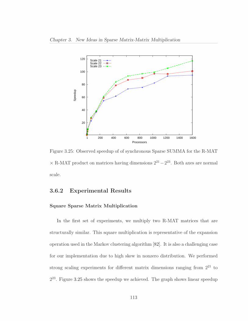
Chapter 3. New Ideas in Sparse Matrix-Matrix Multiplication
20
40
60
80
100
120
1 200 400 600 800 1000 1200 1400 1600
Spe
edup
Processors
Scale 21Scale 22Scale 23
Figure 3.25: Observed speedup of of synchronous Sparse SUMMA for the R-MAT
× R-MAT product on matrices having dimensions 221−223. Both axes are normal
scale.
3.6.2 Experimental Results
Square Sparse Matrix Multiplication
In the first set of experiments, we multiply two R-MAT matrices that are
structurally similar. This square multiplication is representative of the expansion
operation used in the Markov clustering algorithm [82]. It is also a challenging case
for our implementation due to high skew in nonzero distribution. We performed
strong scaling experiments for different matrix dimensions ranging from 221 to
223. Figure 3.25 shows the speedup we achieved. The graph shows linear speedup
113
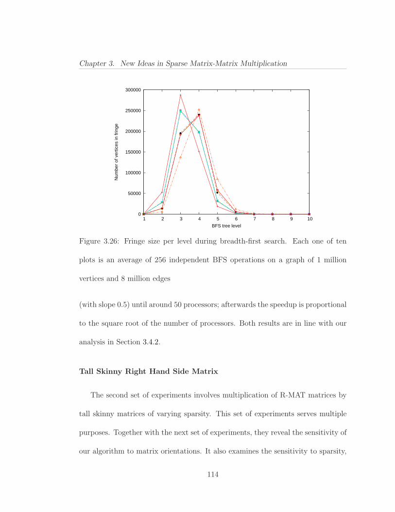
Chapter 3. New Ideas in Sparse Matrix-Matrix Multiplication
0
50000
100000
150000
200000
250000
300000
1 2 3 4 5 6 7 8 9 10
Num
ber
of v
ertic
es in
frin
ge
BFS tree level
Figure 3.26: Fringe size per level during breadth-first search. Each one of ten
plots is an average of 256 independent BFS operations on a graph of 1 million
vertices and 8 million edges
(with slope 0.5) until around 50 processors; afterwards the speedup is proportional
to the square root of the number of processors. Both results are in line with our
analysis in Section 3.4.2.
Tall Skinny Right Hand Side Matrix
The second set of experiments involves multiplication of R-MAT matrices by
tall skinny matrices of varying sparsity. This set of experiments serves multiple
purposes. Together with the next set of experiments, they reveal the sensitivity of
our algorithm to matrix orientations. It also examines the sensitivity to sparsity,
114

Chapter 3. New Ideas in Sparse Matrix-Matrix Multiplication
because we vary the sparsity of the right hand side matrix. Lastly, it is represen-
tative of the parallel breadth-first search that lies in the heart of our betweenness
centrality implementation in Section 5.1. We varied the sparsity of the right hand
side matrix from approximately 1 nonzero per column to 105 nonzeros per column,
with multiplicative increments of 10. Our reasoning is application driven: at each
level of breadth-first search, the current frontier (fringe) has as low as a few ver-
tices but it can have as high as 300000 vertices. Figure 3.26 plots the number of
vertices in the fringe at each level of the breadth-first search for 10 different runs
(with different starting vertices) on a network of 1 million vertices and 8 million
edges.
For our experiments, the R-MAT matrices on the left hand side have c1 = 8
nonzeros per column and their dimensions vary from n = 220 to n = 226. The
right hand side matrix is of size n-by-k, and its number of nonzeros per column, c2
is varied from 1 to 105, with multiplicative increments of 10. Its width, k, varies
from 128 to 8192 that grows proportionally to its length n. Hence, the total work
is W = O(c1c2k), the total memory consumption is M = O(c1n + c2k), and total
bandwidth requirement is is O(M√
p).
We performed scaled speedup experiments where keep both n/p = 214 and
k/p = 2 constant. This way, we were able to keep both memory consumption per
115

Chapter 3. New Ideas in Sparse Matrix-Matrix Multiplication
processor and work per processor constant at the same time. However, bandwidth
requirements per processor increases by a factor of√
p.
Figure 3.27 shows the three-dimensional performance graph. The timings for
each slice along the XZ-plane (i.e. for every c2 = 1, 10, ..., 105 contour), is nor-
malized to its running time on p = 64 processors. We do not cross-compare the
absolute performances using different c2 values, as our focus in this section is par-
allel scaling. The graph demonstrates that, except for the outlier case c2 = 1000,
we achieve the expected√
p slowdown due to communication costs. The perfor-
mance we achieved for these large scale experiments, where we ran our code on
up to 4096 processors, is remarkable.
Multiplication with the Restriction Operator
The multilevel method is widely used in the solution of numerical and com-
binatorial problems [194]. The method constructs smaller problems by successive
coarsening of the problem domain. The simplest coarsening is perhaps graph con-
traction. One contraction step chooses two or more vertices in the original graph
G to become a single aggregate vertex in the contracted graph G′. The edges of G
that used to be incident to any of the vertices forming the aggregate now become
incident to the new aggregate vertex in G′.
116
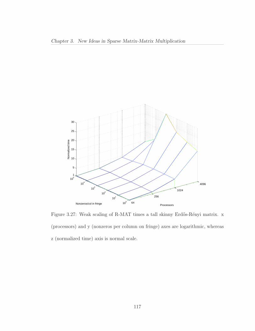
Chapter 3. New Ideas in Sparse Matrix-Matrix Multiplication
64
256
1024
4096
100
101
102
103
104
1051
5
10
15
20
25
30
ProcessorsNonzeros/col in fringe
Nor
mal
ized
tim
e
Figure 3.27: Weak scaling of R-MAT times a tall skinny Erdos-Renyi matrix. x
(processors) and y (nonzeros per column on fringe) axes are logarithmic, whereas
z (normalized time) axis is normal scale.
117

Chapter 3. New Ideas in Sparse Matrix-Matrix Multiplication
Constructing a coarser grid during the V-cycle of the Algebraic Multigrid
(AMG) method [42] or graph partitioning [118] is a generalized graph contraction
operation. Different algorithms need different coarsening operators. For example,
a weighted (as opposed to strict) aggregation [58] might be preferred for parti-
tioning problems. In general, coarsening can be represented as multiplication of
the matrix representing the original fine domain (grid, graph, or hypergraph) by
the restriction operator.
In this experiments, we use a simple restriction operation to perform graph con-
traction. Gilbert et al. [105] describe how to perform contraction using SpGEMM.
Their elegant algorithm creates a special sparse matrix S with n nonzeros. The
triple product SAST contracts the whole graph at once. Making S smaller in the
first dimension while keeping the number of nonzeros same changes the restriction
order. For example, we contract the graph into half by using S having dimensions
n/2× n, which is said to be of order 2.
Figure 3.28 shows the strong scaling of the operation AST for R-MAT graphs
of scale 23. We used restrictions of order 2, 4, and 8. Changing the interpolation
order results in minor changes in performance. The experiment shows good scaling
for up to 1024 processors.
118
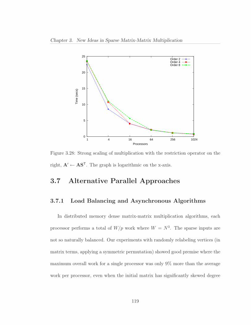
Chapter 3. New Ideas in Sparse Matrix-Matrix Multiplication
0
5
10
15
20
25
1 4 16 64 256 1024
Tim
e (s
ecs)
Processors
Order 2Order 4Order 8
Figure 3.28: Strong scaling of multiplication with the restriction operator on the
right, A′ ← AST. The graph is logarithmic on the x-axis.
3.7 Alternative Parallel Approaches
3.7.1 Load Balancing and Asynchronous Algorithms
In distributed memory dense matrix-matrix multiplication algorithms, each
processor performs a total of W/p work where W = N3. The sparse inputs are
not so naturally balanced. Our experiments with randomly relabeling vertices (in
matrix terms, applying a symmetric permutation) showed good premise where the
maximum overall work for a single processor was only 9% more than the average
work per processor, even when the initial matrix has significantly skewed degree
119
Chapter 3. New Ideas in Sparse Matrix-Matrix Multiplication
distribution1. Aiming for perfect load balance via graph or hypergraph partition-
ing [54, 55, 203] seems impractical whenever the matrices are not reused. Even
when one of the matrices are fixed throughout the computation, load balance for
SpGEMM can not be determined solely based on one operand, unlike SpMV. We
do not know of any applications where both matrix operands have fixed struc-
ture for several subsequent multiplication operations, which might have justified
complex load balancing.
The sparse 2D algorithms presented in previous sections execute in a syn-
chronous manner in s stages in their naive form. For sparse matrices, achiev-
ing good load balance per stage is harder than achieving load balance for the
whole computation. This is because a local submatrix update such as Ci,j ←
Ci,j + Ai,kBk,j might have significantly more work to do than another update at
the same stage, say Ci+1,j ← Ci+1,j + Ai+1,kBk,j. However, in a subsequent stage
the roles of the (i, j)th and the (i+1, j)th processor might swap; hence balancing
the load across stages. On the other hand, a barrier synchronization at each stage
forces everyone to wait for the slowest update until they can proceed to the next
stage. Hence, we expect an asynchronous algorithm to perform better than a
synchronous one for matrices with highly skewed nonzero distribution.
1For sufficiently large matrices on 256 processors, as shown in Figure 3.30
120

Chapter 3. New Ideas in Sparse Matrix-Matrix Multiplication
In order to quantify the severity of load imbalance, we performed a simulation
of the Sparse Cannon algorithm that accounts for the computation (in terms of
the number of actual flops only) and communication (nnz only) done by each
processor. We varied the matrix dimension and the number of processors while
the number of nonzeros per row/column were kept constant. For RMAT matrices
with 8 nonzeros per column, the per-stage load imbalance with 256 processors
is shown in Figure 3.29. Load imbalance is defined as the ratio of the maximum
number of flops performed by any processor to the average number of flops. These
plots are typical in the sense that we permuted the input matrices multiple times
with different random permutations and plotted the results of the permutation
that resulted in the median load imbalance.
Figure 3.30(a) shows the overall load imbalance for increasing matrix sizes on
256 processors. The problem becomes well balanced (i.e. it has less 10% load
imbalance) for R-MAT inputs of scale 20 and larger. On the other hand, Fig-
ure 3.30(b) shows a comparison of the trends of overall and per-stage imbalances
(average over all stages) with increasing number of processors and a fixed problem
size.
These results on Figures 3.29 and 3.30 suggest that per-stage load balance
is significantly harder to achieve than load balance for the overall computation.
Both tend to decrease as the problem size gets bigger, although per-stage load
121

Chapter 3. New Ideas in Sparse Matrix-Matrix Multiplication
1 2 3 4 5 6 7 8 9 10 11 12 13 14 15 16
1.8
1.85
1.9
1.95
2
2.05
2.1
Worst load imbalance by stage
Multiplication stage
(a) RMAT Scale-15
1 2 3 4 5 6 7 8 9 10 11 12 13 14 15 16
2.2
2.25
2.3
2.35
2.4
2.45
2.5
2.55
Worst load imbalance by stage
Multiplication stage
(b) RMAT Scale-16
1 2 3 4 5 6 7 8 9 10 11 12 13 14 15 16
1.54
1.56
1.58
1.6
1.62
1.64
1.66
1.68
Worst load imbalance by stage
Multiplication stage
(c) RMAT Scale-17
1 2 3 4 5 6 7 8 9 10 11 12 13 14 15 16
1.52
1.54
1.56
1.58
1.6
1.62
Worst load imbalance by stage
Multiplication stage
(d) RMAT Scale-18
1 2 3 4 5 6 7 8 9 10 11 12 13 14 15 16
1.56
1.58
1.6
1.62
1.64
1.66
1.68
1.7
1.72
Worst load imbalance by stage
Multiplication stage
(e) RMAT Scale-19
1 2 3 4 5 6 7 8 9 10 11 12 13 14 15 16
1.4
1.45
1.5
1.55
Worst load imbalance by stage
Multiplication stage
(f) RMAT Scale-20
Figure 3.29: Load imbalance per stage for multiplying two RMAT matrices on256 processors using Sparse Cannon
122
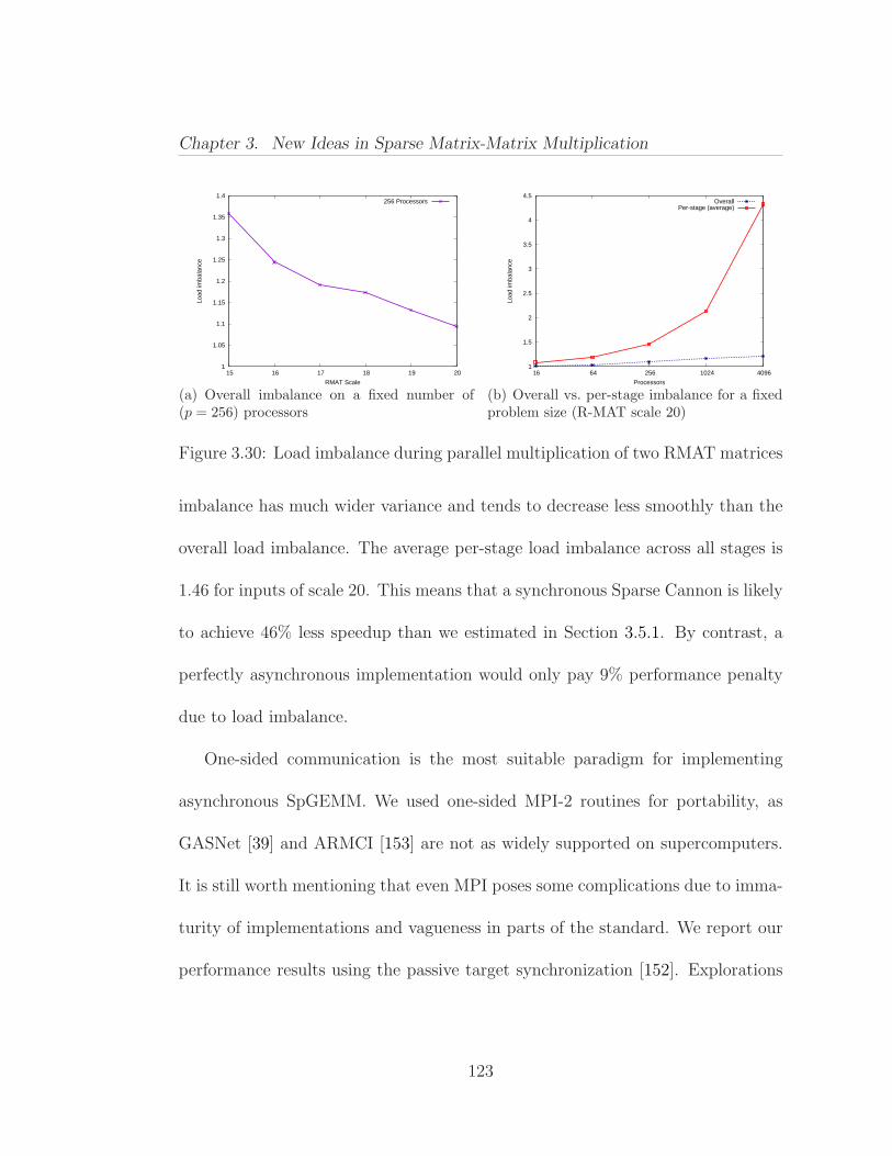
Chapter 3. New Ideas in Sparse Matrix-Matrix Multiplication
1
1.05
1.1
1.15
1.2
1.25
1.3
1.35
1.4
15 16 17 18 19 20
Load
imba
lanc
e
RMAT Scale
256 Processors
(a) Overall imbalance on a fixed number of(p = 256) processors
1
1.5
2
2.5
3
3.5
4
4.5
16 64 256 1024 4096
Load
imba
lanc
e
Processors
OverallPer-stage (average)
(b) Overall vs. per-stage imbalance for a fixedproblem size (R-MAT scale 20)
Figure 3.30: Load imbalance during parallel multiplication of two RMAT matrices
imbalance has much wider variance and tends to decrease less smoothly than the
overall load imbalance. The average per-stage load imbalance across all stages is
1.46 for inputs of scale 20. This means that a synchronous Sparse Cannon is likely
to achieve 46% less speedup than we estimated in Section 3.5.1. By contrast, a
perfectly asynchronous implementation would only pay 9% performance penalty
due to load imbalance.
One-sided communication is the most suitable paradigm for implementing
asynchronous SpGEMM. We used one-sided MPI-2 routines for portability, as
GASNet [39] and ARMCI [153] are not as widely supported on supercomputers.
It is still worth mentioning that even MPI poses some complications due to imma-
turity of implementations and vagueness in parts of the standard. We report our
performance results using the passive target synchronization [152]. Explorations
123
Chapter 3. New Ideas in Sparse Matrix-Matrix Multiplication
on different one-sided approaches and issues associated with them can be found
in Appendix A.
MPI-1 standard is inadequate to address the asynchronous implementation
challenge. The blocking operations do trivially synchronize, and the non-blocking
operations buffer the message and revert to a synchronous mode whenever the data
is too large to fit in the buffers [172]. The basic requirement of an asynchronous
SpGEMM is that the (i, j)th processor should be able to fetch its required subma-
trix from its original owner regardless of its computation stage at that moment.
Although this can be achieved by the use of a helper thread that waits on the
Send() operation, ready to serve any incoming Recv() requests, this approach has
two drawbacks. Firstly, there is a substantial performance loss due to oversub-
scribing the processor. Secondly, general multithreaded MPI support is still in its
infancy2.
3.7.2 Overlapping Communication with Computation
In order to hide communication costs as much as possible, each processor starts
prefetching one submatrix ahead while computing its current submatrix product.
More concretely, processor P (i, j) starts prefetching Ai,k+1 and Bk+1,j while com-
puting Ai,kBk,j. To keep the memory footprint the same as the synchronous
2OpenMPI’s MPI THREAD MULTIPLE support, which failed in our tests, is known to beuntested
124
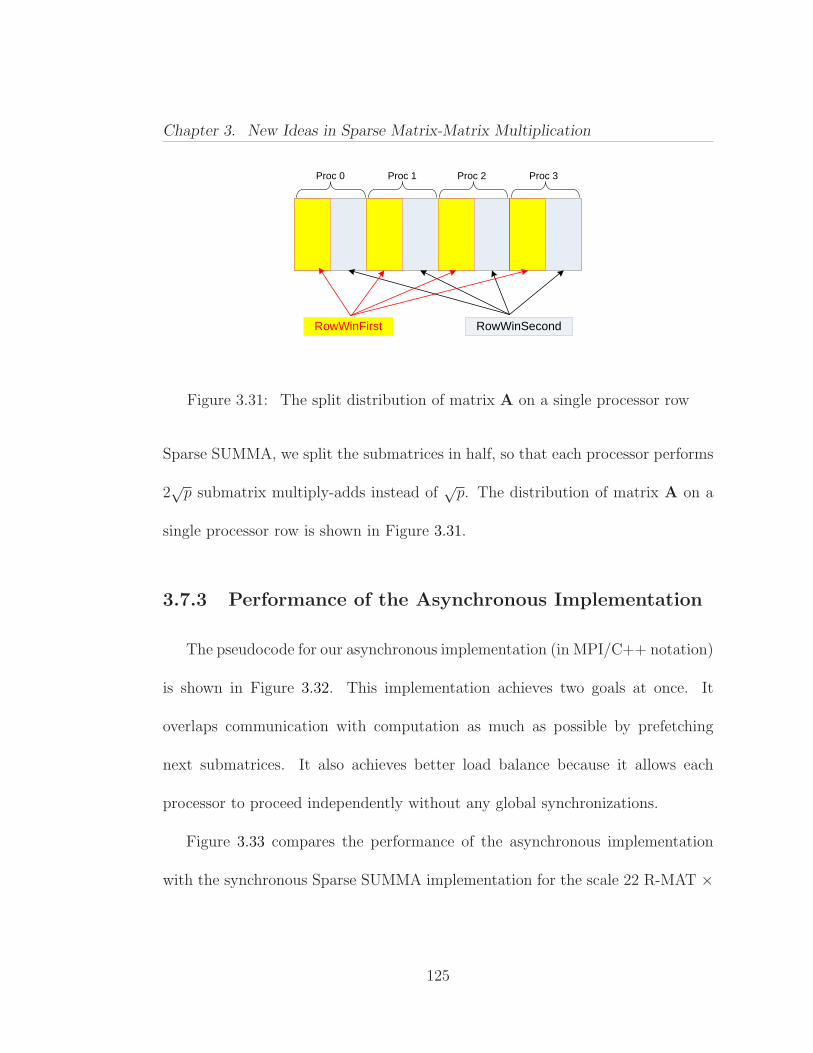
Chapter 3. New Ideas in Sparse Matrix-Matrix Multiplication
RowWinFirst RowWinSecond
Proc 0 Proc 1 Proc 2 Proc 3
Figure 3.31: The split distribution of matrix A on a single processor row
Sparse SUMMA, we split the submatrices in half, so that each processor performs
2√
p submatrix multiply-adds instead of√
p. The distribution of matrix A on a
single processor row is shown in Figure 3.31.
3.7.3 Performance of the Asynchronous Implementation
The pseudocode for our asynchronous implementation (in MPI/C++ notation)
is shown in Figure 3.32. This implementation achieves two goals at once. It
overlaps communication with computation as much as possible by prefetching
next submatrices. It also achieves better load balance because it allows each
processor to proceed independently without any global synchronizations.
Figure 3.33 compares the performance of the asynchronous implementation
with the synchronous Sparse SUMMA implementation for the scale 22 R-MAT ×
125
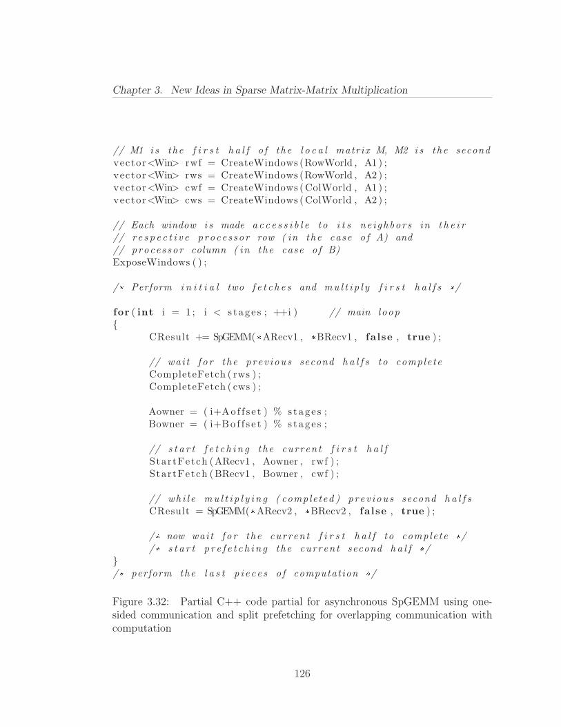
Chapter 3. New Ideas in Sparse Matrix-Matrix Multiplication
// M1 i s the f i r s t h a l f o f the l o c a l matrix M, M2 i s the secondvector<Win> rwf = CreateWindows (RowWorld , A1 ) ;vector<Win> rws = CreateWindows (RowWorld , A2 ) ;vector<Win> cwf = CreateWindows (ColWorld , A1 ) ;vector<Win> cws = CreateWindows (ColWorld , A2 ) ;
// Each window i s made a c c e s s i b l e to i t s ne i ghbors in t h e i r// r e s p e c t i v e proces sor row ( in the case o f A) and// proces sor column ( in the case o f B)ExposeWindows ( ) ;
/* Perform i n i t i a l two f e t c h e s and mu l t i p l y f i r s t h a l f s */for ( int i = 1 ; i < s t ag e s ; ++i ) // main loop
CResult += SpGEMM(*ARecv1 , *BRecv1 , false , true ) ;
// wai t f o r the prev ious second h a l f s to completeCompleteFetch ( rws ) ;CompleteFetch ( cws ) ;
Aowner = ( i+Ao f f s e t ) % s tage s ;Bowner = ( i+Bo f f s e t ) % s tage s ;
// s t a r t f e t c h i n g the current f i r s t h a l fStartFetch (ARecv1 , Aowner , rwf ) ;StartFetch (BRecv1 , Bowner , cwf ) ;
// wh i l e mu l t i p l y i n g ( completed ) prev ious second h a l f sCResult = SpGEMM(*ARecv2 , *BRecv2 , false , true ) ;
/* now wai t f o r the current f i r s t h a l f to complete *//* s t a r t p r e f e t c h i n g the current second h a l f */
/* perform the l a s t p i e c e s o f computation */Figure 3.32: Partial C++ code partial for asynchronous SpGEMM using one-sided communication and split prefetching for overlapping communication withcomputation
126
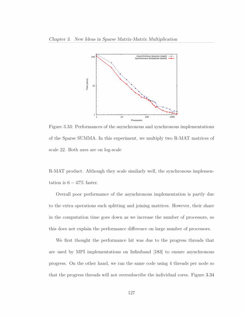
Chapter 3. New Ideas in Sparse Matrix-Matrix Multiplication
1
10
100
1 10 100 1000
Tim
e (s
ecs)
Processors
Asynchronous (passive target)Synchronous (broadcast based)
Figure 3.33: Performances of the asynchronous and synchronous implementations
of the Sparse SUMMA. In this experiment, we multiply two R-MAT matrices of
scale 22. Both axes are on log-scale
R-MAT product. Although they scale similarly well, the synchronous implemen-
tation is 6− 47% faster.
Overall poor performance of the asynchronous implementation is partly due
to the extra operations such splitting and joining matrices. However, their share
in the computation time goes down as we increase the number of processors, so
this does not explain the performance difference on large number of processors.
We first thought the performance hit was due to the progress threads that
are used by MPI implementations on Infiniband [183] to ensure asynchronous
progress. On the other hand, we ran the same code using 4 threads per node so
that the progress threads will not oversubscribe the individual cores. Figure 3.34
127
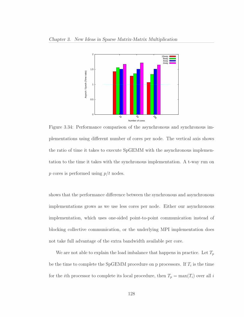
Chapter 3. New Ideas in Sparse Matrix-Matrix Multiplication
0
0.5
1
1.5
2
16 64 256
Asy
nch
/ Syn
ch (
Tim
e ra
tio)
Number of cores
16way8way4way2way
Figure 3.34: Performance comparison of the asynchronous and synchronous im-
plementations using different number of cores per node. The vertical axis shows
the ratio of time it takes to execute SpGEMM with the asynchronous implemen-
tation to the time it takes with the synchronous implementation. A t-way run on
p cores is performed using p/t nodes.
shows that the performance difference between the synchronous and asynchronous
implementations grows as we use less cores per node. Either our asynchronous
implementation, which uses one-sided point-to-point communication instead of
blocking collective communication, or the underlying MPI implementation does
not take full advantage of the extra bandwidth available per core.
We are not able to explain the load imbalance that happens in practice. Let Tp
be the time to complete the SpGEMM procedure on p processors. If Ti is the time
for the ith processor to complete its local procedure, then Tp = max(Ti) over all i
128

Chapter 3. New Ideas in Sparse Matrix-Matrix Multiplication
due to wait times. For the asychronous implementation, our preliminary profiling
(on 256 cores) revealed that the fastest processor spends more time waiting for the
other processors than doing useful computation. On average, a processor spent
about 1/3rd of its time waiting.
The slowdown due to the asynchronous execution was previously experienced
on the Connection Machine CM5 [139] on programs with regular communication
patterns. Brewer and Kuszmaul [41] found out that an initial skew of processors
slowed down the overall computation on the CM5, as receiver queues started to
back off. The CM-5 data network is similar to Ranger’s, in the sense that they
both use a fat-tree [137] interconnect. However, the problem with the CM-5 was
the contention on the receivers due to the computational cost of receiving packets.
Ranger’s Infiniband interconnect, on the other hand, has RDMA support for this
task. However, we do not know whether MPI-2 functions have been implemented
to fully take advantage of the network’s capabilities. In conclusion, revealing the
exact cause of the poorer performance of the asynchronous implementation needs
further research and more performance profiling.
129
Chapter 3. New Ideas in Sparse Matrix-Matrix Multiplication
3.8 Future Work
Our mathematical modeling of the parallel algorithms in Section 3.3 is an
average-case analysis assuming independent uniform random distribution of nonze-
ros, which translates into the Erdos-Renyi random graph model. More realistic
models should assume skewed nonzero distributions, such as power-law distribu-
tions. Ultimately, average case analysis has its limitations because it needs to
assume an underlying distribution. On the other hand, worst case analysis does
not make a lot of sense for our problem, because there are certain sparse matrix
pairs that will create a dense output when multiplied. Therefore, a smoothed
analysis [186] of the sparse matrix multiplication algorithms, both sequentially
and in parallel, would be a significant advancement.
Load imbalance is not severe for sufficiently large matrices, even in the absence
of asynchronous progress. Our one-sided communication approach was based on
remote get operations in order to avoid fence synchronization. Given the accept-
able load balance for large matrices, it is worth exploring an option with fence
synchronization and remote put operations. This proposed implementation will
still use one-sided communication but all processors in the processor row/column
will need to synchronize after the put operation. We expect better performance
130
Chapter 3. New Ideas in Sparse Matrix-Matrix Multiplication
because it only takes one trip to complete a remote put operation whereas remote
get requires a roundtrip.
Our SpGEMM routine might be extended to handle matrix chain products.
In particular, the sparse matrix triple product (RAP) is heavily used in the coars-
ening phase of the algebraic multigrid method [4]. Sparse matrix indexing and
parallel graph contraction also require sparse matrix triple product [105]. The sup-
port for sparse matrix chain products eliminates temporary intermediate products
and allows more optimizations, such as performing structure prediction [63] and
finding the optimal parenthesization based on the sparsity of the inputs.
Finally, there is a need for hierarchical parallelism due to vast differences in
the costs of inter-node and intra-node communication. The flat parallelism model
does not only lose the opportunity to exploit the faster on-chip network, but it also
increases the contention on the off-chip links. We observed that the inter-node
communication becomes slower as the number of cores per node increases because
more processes are competing for the same network link. Therefore, designing a
hierarchically parallel Sparse GEMM algorithm is an important future direction.
131
Chapter 4
The Combinatorial BLAS: Designand Implementation
My impression was and is that many programming languages and toolsrepresent solutions looking for problems, and I was determined that mywork should not fall into that category
Bjarne Stroustrup
The Combinatorial BLAS library is a parallel library for graph computations.
It is intented to provide a common interface for high-performance graph kernels.
It is unique among other graph libraries for combining scalability with distributed
memory parallelism. We borrowed ideas from the domain of parallel numerical
analysis and applied them to parallel graph computations.
4.1 Motivation
The Matlab reference implementation of the HPCS Scalable Synthetic Com-
pact Applications graph analysis (SSCA#2) benchmark was an important step
132
Chapter 4. The Combinatorial BLAS: Design and Implementation
towards using linear algebra operations for implementing graph algorithms. Al-
though it was a success in terms of expressibility and ease of implementation, its
performance was about 50% worse than the best serial implementation. Mostly,
the slowdown was due to limitations of Matlab for performing integer operations
1. The parallel scaling was also limited on most parallel Matlab implementations.
The idea of having a BLAS-like library for doing graph computation is driven
by the desire to create a general purpose library that supports rapid implemen-
tation of graph algorithms using a small yet important subset of linear algebra
operations. The library should also be in parallel and scale well due to the massive
size of graphs in many modern applications.
4.2 Design Philosophy
4.2.1 The Overall Design
The first class citizens of the Combinatorial BLAS are distributed sparse ma-
trices. Application domain interactions that are abstracted into a graph are con-
cretely represented as a sparse matrix. Therefore, all non-auxiliary functions are
designed to operate on sparse matrix objects. There are three other types of
objects that are used by some of the functions: dense matrices, dense vectors,
1Matlab does not support integer data elements for its sparse matrices
133
Chapter 4. The Combinatorial BLAS: Design and Implementation
sparse vectors. Concrete data structures for these objects are explained in detail
in Section 4.3.
We follow some of the guiding design principles of the popular and successful
PETSc package [21]. We achieve extensibility by defining a common abstraction
for all sparse matrix storage formats, making it possible to implement a new
format and plug it in without changing rest of the library. For scalability, it is
possible (and encouraged) to create objects by passing special MPI communicator
objects instead of using the default COMM::WORLD object that includes all the
processes in the system. This use of communicators also helps to avoid inter-
library and intra-library collisions. We do not attempt to create the illusion of
a flat address space; communication is internally handled by parallel classes of
the library. Likewise, we do not always provide storage independence due to
our emphasis on high performance. Some operations have different semantics
depending on whether the underlying object is sparse or dense.
The Combinatorial BLAS routines (API functions) are supported both sequen-
tially and in parallel. The communication is managed within the parallel versions
(i.e. , versions operating on parallel objects) of these high-level operations, which
call the sequential versions for computation on local data. This symmetry of func-
tion prototypes has a nice effect on interoperability. The parallel objects can just
treat their internally stored sequential objects as black boxes supporting the API
134

Chapter 4. The Combinatorial BLAS: Design and Implementation
functions. Conversely, any sequential class becomes fully compatible with the rest
of the library as long as it supports the API functions and allows access to its
internal arrays through an adapter object. This decoupling of parallel logic from
sequential parts of the computation is one of the distinguishing features of the
Combinatorial BLAS.
4.2.2 The Combinatorial BLAS Routines
We selected the operations to be supported by the API by a top-down, ap-
plication driven process. Commonly occurring computational patterns in many
graph algorithms are abstracted into a few linear algebraic kernels that can be
efficiently mapped into the architecture of distributed memory computers. The
API is not intended to be final and will be extended as more applications are
analyzed and new algorithms are invented.
We address the tension between generality and performance by the zero over-
head principle: Our primary goal is to provide work-efficiency for the targeted
graph algorithms. The interface is kept general, simple, and clean so long as doing
so does not add significant overhead to the computation. The guiding principles
in the design of the API are listed below, each one illustrated with an example.
(1) If multiple operations can be handled by a single function prototype without
degrading the asymptotic performance of the algorithm they are to be part
135
Chapter 4. The Combinatorial BLAS: Design and Implementation
of, then we provide a generalized single prototype. Otherwise, we provide
multiple prototypes.
For example, it is tempting to define a single function prototype for elemen-
twise operations on sparse matrices. Although it seems achievable by passing
a binop parameter, semantics of sparse matrices differ depending on the binary
operation. For instance, ignoring numerical cancellation, elementwise addition is
most efficiently implemented as a union of two sets while multiplication is the in-
tersection. Other elementwise operations between two sparse matrices are handled
similarly, but using different functions. If it proves to be efficiently implementable
(using either function object traits or run-time type information), all elementwise
operations between two sparse matrices may have a single function prototype in
the future.
On the other hand, the data access patterns of matrix-matrix and matrix-
vector multiplications are independent of the underlying semiring. In fact, many
connectivity problems use the Boolean semiring (0, 1,∨,∧, 0, 1) and many short-
est path algorithms use the tropical semiring (R+, min, +,∞, 0). As a result, the
sparse matrix-matrix multiplication routine SpGEMM and the sparse matrix-
vector multiplication routine SpMV accept a parameter representing the semir-
ing. The SpGEMM function also expects two additional parameters, trA and trB,
136

Chapter 4. The Combinatorial BLAS: Design and Implementation
and depending on those, computes one of the following operations: C ← A · B,
C← AT ·B, C← A ·BT, C← AT ·BT.
(2) If an operation can be efficiently implemented by composing a few simpler
operations, then we do not provide a special function for that operator.
For example, making a nonzero matrix A column stochastic can be efficiently
implemented by first calling Reduce on A to get a dense row vector v that
contains the sums of columns, then obtaining the multiplicative inverse of each
entry in v by calling the Apply function with the unary function object that
performs f(vi) = 1/vi for every vi it is applied to, and finally calling Scale(v) on
A to effectively divide each nonzero entry in a column by its sum. Consequently,
we do not provide a special function to make a matrix column stochastic.
On the other hand, a commonly occurring operation is to zero out some of
the nonzeros of a sparse matrix. This often comes up in graph traversals, where
Xk represents the set of vertices that are discovered during the kth iteration (i.e.
the kth frontier). Multiplying Xk by the adjacency matrix of the graph yields
another matrix that might include some of the previously discovered vertices in
addition to the set of vertices that are discovered during the (k + 1)st iteration.
Those old vertices need to be pruned from the frontier before starting the next
iteration. One way to implement this pruning operation is to keep a matrix Y
that includes a zero for every vertex that has been discovered before, and nonzeros
137
Chapter 4. The Combinatorial BLAS: Design and Implementation
elsewhere. Performing an elementwise multiplication with Y yields the desired
frontiers matrix Xk+1. However, this approach might not be work-efficient since
Y will often be dense, especially in the early stages of the graph traversal.
Consequently, we provide a generalized function SpEWiseX that performs the
elementwise multiplication of sparse matrices op(A) and op(B). It also accepts
two auxiliary parameters, notA and notB, that are used to negate the sparsity
structure of A and B. If notA is true, then op(A)(i, j) = 0 for every nonzero
A(i, j) 6= 0 and op(A)(i, j) = 1 for every zero A(i, j) = 0. The role of notB is
identical. Direct support for the logical NOT operations is crucial to avoid the
explicit construction of the dense not(B) object.
(3) To avoid expensive object creation and copying, many functions also have
in-place versions. For operations that can be implemented in place, we deny
access to any other variants only if those increase the running time.
For example, Scale(B) is a member function of the sparse matrix class that
takes a dense matrix as a parameter. When called on the sparse matrix A, it
replaces each A(i, j) 6= 0 with A(i, j) · B(i, j). This operation is implemented
only in-place because B(i, j) is guaranteed to exist for a dense matrix, allowing
us to perform a single scan of the nonzeros of A and update them by doing fast
lookups on B. Not all elementwise operations can be efficiently implemented in-
place (for example elementwise addition of a sparse matrix and a dense matrix will
138
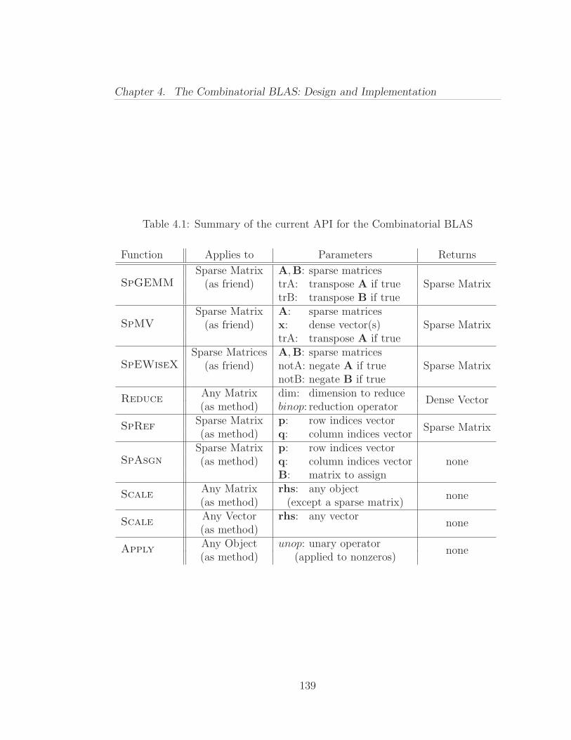
Chapter 4. The Combinatorial BLAS: Design and Implementation
Table 4.1: Summary of the current API for the Combinatorial BLAS
Function Applies to Parameters Returns
SpGEMM
Sparse Matrix A,B: sparse matricesSparse Matrix(as friend) trA: transpose A if true
trB: transpose B if true
SpMV
Sparse Matrix A: sparse matricesSparse Matrix(as friend) x: dense vector(s)
trA: transpose A if true
SpEWiseX
Sparse Matrices A,B: sparse matricesSparse Matrix(as friend) notA: negate A if true
notB: negate B if true
ReduceAny Matrix dim: dimension to reduce
Dense Vector(as method) binop: reduction operator
SpRefSparse Matrix p: row indices vector
Sparse Matrix(as method) q: column indices vector
SpAsgn
Sparse Matrix p: row indices vectornone(as method) q: column indices vector
B: matrix to assign
ScaleAny Matrix rhs: any object
none(as method) (except a sparse matrix)
ScaleAny Vector rhs: any vector
none(as method)
ApplyAny Object unop: unary operator
none(as method) (applied to nonzeros)
139

Chapter 4. The Combinatorial BLAS: Design and Implementation
produce a dense matrix), so the implementer is free to declare them as members of
the dense matrix class or declare them as global functions returning a new object.
(4) In-place operations have slightly different semantics depending on whether
the operands are sparse or dense. In particular, the semantics favor leav-
ing the sparsity pattern of the underlying object intact as long as another
function (possibly not in-place) handles the more conventinal semantics that
introduces/deletes nonzeros.
For example, Scale is an overloaded method, available for all objects. It
does not destroy sparsity when called on sparse objects and it does not introduce
sparsity when called on dense objects. The semantics of the particular Scale
method is dictated by its the class object and its operand. Called on a sparse
matrix A with a vector v, it independently scales nonzero columns (or rows) of
the sparse matrix. For v being a row vector 2, Scale replaces every nonzero
A(i, j) with v(j) ·A(i, j). The parameter v can be dense or sparse. In the latter
case, only a portion of the sparse matrix is scaled. That is, v(j) being zero for a
sparse vector does not zero out the corresponding jth column of A. The Scale
operation never deletes columns from A; deletion of columns is handled by the
more expensive SpAsgn function.
2Row/column vector distinction changes the semantics only. Row and column vectors (evendistributed versions) are stored the same way.
140
Chapter 4. The Combinatorial BLAS: Design and Implementation
SpAsgn and SpRef are generalized sparse matrix assignment and indexing
operations. They are very powerful primitives that take vectors p and q of row
and column indices. When called on the sparse matrix A, SpRef returns a new
sparse matrix whose rows are the p(i)th rows of A for i = 0, ..., length(p)−1 and
whose columns are the q(j)th columns of A for j = 0, ..., length(q)−1. SpAsgn
has similar syntax, except that it returns a reference (an modifiable lvalue) to some
portion of the underlying object as opposed to returning a new object. Internally,
the implementer is free (and encouraged) to use different subroutines for special
cases such as row-wise (A(i, :)), column-wise (A(:, j)), and element-wise (A(i, j))
indexing/assignment.
4.3 A Reference Implementation
4.3.1 The Software Architecture
In our reference implementation, the main data structure is a distributed sparse
matrix object SpDistMat which HAS-A local sparse matrix that can be imple-
mented in various ways as long as it supports the interface of the base class
SpMat . All features regarding distributed-memory parallelization, such as the
communication patterns and schedules, are embedded into the distributed ob-
jects (sparse and dense) through the CommGrid object. Global properties of
141

Chapter 4. The Combinatorial BLAS: Design and Implementation
distributed objects, such as the total number of nonzeros and the overall matrix
dimensions, are not explicitly stored. They are computed by reduction operations
whenever necessary. The software architecture for matrices is illustrated in Fig-
ure 4.1. Although the inheritance relationships are shown in the traditional way
(via inclusion polymorphism [53]), the class hierarchies are static, obtained by the
parameterizing the base class with its subclasses as explained below.
!"! #!"! $%&'()* !"+
"',-. "'#&*.,-. #)/*)#&*.,-.
#&*.,-.!0112%&3
Figure 4.1: Software architecture for matrix classes
To enforce a common interface as defined by the API, all types of objects derive
from their corresponding base classes. The base classes only serve to dictate the
interface. This is achieved through static object oriented programming (OOP)
techniques [51] rather than expensive dynamic dispatch. A trick known as the
142
Chapter 4. The Combinatorial BLAS: Design and Implementation
Curiously Recurring Template Pattern (CRTP) [66] emulates dynamic dispatch
statically, with some limitations. These limitations, such as the inability to use
heterogeneous lists of objects that share the same type class, however, are not
crucial for the Combinatorial BLAS. In CRTP, the base class accepts a template
parameter of the derived class.
The SpMat base class implementation is given as an example in Figure 4.2.
As all exact types are known at compile time, there are no runtime overheads
arising from dynamic dispatch. In the presence of covariant arguments, static
polymorphism through CRTP automatically allows for better type checking of
parameters. In the SpGEMM example, with classical OOP, one would need to
dynamically inspect the actual types of A and B to see whether they are compati-
ble; and if they are, to call the right subroutines. This requires expensive run-time
type information queries and dynamic cast() operations. More problematically, it
is unsafe, as any unconforming set of parameters will lead to a run-time error or
an exception. Static OOP catches any such incompatibilities in compile time.
The SpMat object is local to a node but it need not be sequential. It can
be implemented as a shared-memory data structure, amenable to thread-level
parallelization. This flexibility will allow future versions of the Combinatorial
BLAS algorithms to support hybrid parallel programming paradigms. The main
distinguishing feature of SpMat is the contiguous storage of its sparse matrix,
143
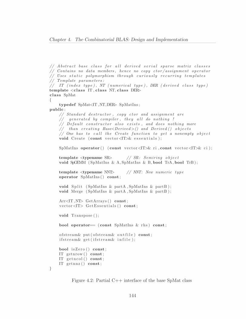
Chapter 4. The Combinatorial BLAS: Design and Implementation
// Abs t rac t base c l a s s f o r a l l d e r i v ed s e r i a l sparse matrix c l a s s e s// Contains no data members , hence no copy c to r / assignment opera tor// Uses s t a t i c polymorphism through cu r i o u s l y r ecur r ing t emp la t e s// Template parameters :// IT ( index type ) , NT ( numerical type ) , DER ( der i v ed c l a s s type )template <class IT , class NT, class DER>class SpMat
typedef SpMat<IT ,NT,DER> SpMatIns ;public :
// Standard de s t ruc to r , copy c to r and assignment are// generated by compi ler , they a l l do noth ing !// De fau l t cons t ruc t o r a l s o e x i s t s , and does noth ing more// than c r ea t i n g Base<Derived >() and Derived () o b j e c t s// One has to c a l l the Create func t i on to ge t a nonempty o b j e c tvoid Create ( const vector<IT>& e s s e n t i a l s ) ;
SpMatIns operator ( ) ( const vector<IT>& r i , const vector<IT>& c i ) ;
template <typename SR> // SR: Semiring o b j e c tvoid SpGEMM ( SpMatIns & A, SpMatIns & B, bool TrA, bool TrB ) ;
template <typename NNT> // NNT: New numeric typeoperator SpMatIns ( ) const ;
void Sp l i t ( SpMatIns & partA , SpMatIns & partB ) ;void Merge ( SpMatIns & partA , SpMatIns & partB ) ;
Arr<IT ,NT> GetArrays ( ) const ;vector<IT> GetEs s en t i a l s ( ) const ;
void Transpose ( ) ;
bool operator== ( const SpMatIns & rhs ) const ;
o f s tream& put ( ofstream& o u t f i l e ) const ;i f s t r e am& get ( i f s t r e am& i n f i l e ) ;
bool i sZ e r o ( ) const ;IT getnrow ( ) const ;IT ge tnco l ( ) const ;IT getnnz ( ) const ;
Figure 4.2: Partial C++ interface of the base SpMat class
144
Chapter 4. The Combinatorial BLAS: Design and Implementation
making it accessible by all other components (threads/processes). In this regard,
it is different from the SpDistMat, which distributes the storage of its sparse
matrices.
We observe that the commonality between all sparse matrix storage formats
is their use of multiple arrays. Therefore, the parallel classes handle object creat-
ing and communication through what we call an Essentials object, which is an
adapter for the actual sparse matrix object. The Essentials of a sparse matrix ob-
ject is its dimensions, number of nonzeros, starting addresses of its internal arrays
and the sizes of those arrays. Through GetEssentials() and Create(Essentials ess)
functions, any SpDistMat object can internally have any SpMat object. For ex-
ample, communication can be overlapped with computation in the SpGEMM
function by prefetching the internal arrays through one sided communication.
Alternatively, another SpDistMat class that uses a completely different communi-
cation library, such as GASNet [39] or ARMCI [153], can be implemented without
requiring any changes to the sequential SpMat object.
Most combinatorial operations use more than the traditional floating-point
arithmetic, with integer and boolean operations being prevalent. To provide the
user the flexibility to define their objects (matrices and vectors) with any scalar
type, all of our classes and functions are templated. A practical issue is to be
able perform operations between two objects holding different scalar types, e.g.,
145
Chapter 4. The Combinatorial BLAS: Design and Implementation
multiplication of a boolean sparse matrix by an integer sparse matrix. Explicit
upcasting of one of the operands to a temporary object might have jeopardized
performance due to copying of such big objects. The template mechanism of C++
provided a neat solution to the mixed mode arithmetic problem by providing
automatic type promotion through trait classes [25]. Arbitrary semiring support
for matrix-matrix and matrix-vector products is allowed by passing a class (with
static add and multiply functions) as a template parameter to corresponding
SpGEMM and SpMV functions.
4.3.2 Management of Distributed Objects
The processors are logically organized as a two-dimensional grid in order to
limit most of the communication to take place along a processor column or row
with√
p processors, instead of communicating potentially with all p processors.
The partitioning of distributed matrices (sparse and dense) follows this processor
grid organization, using a 2D block decomposition, also called the checkerboard
partitioning [107]. Figure 4.3 shows this for the sparse case.
Portions of dense matrices are stored locally as two dimensional dense arrays
in each processor. Sparse matrices (SpDistMat objects), on the other hand, have
many possible representations, and the right representation depends on the partic-
ular setting or the application. The problems with using the popular compressed
146
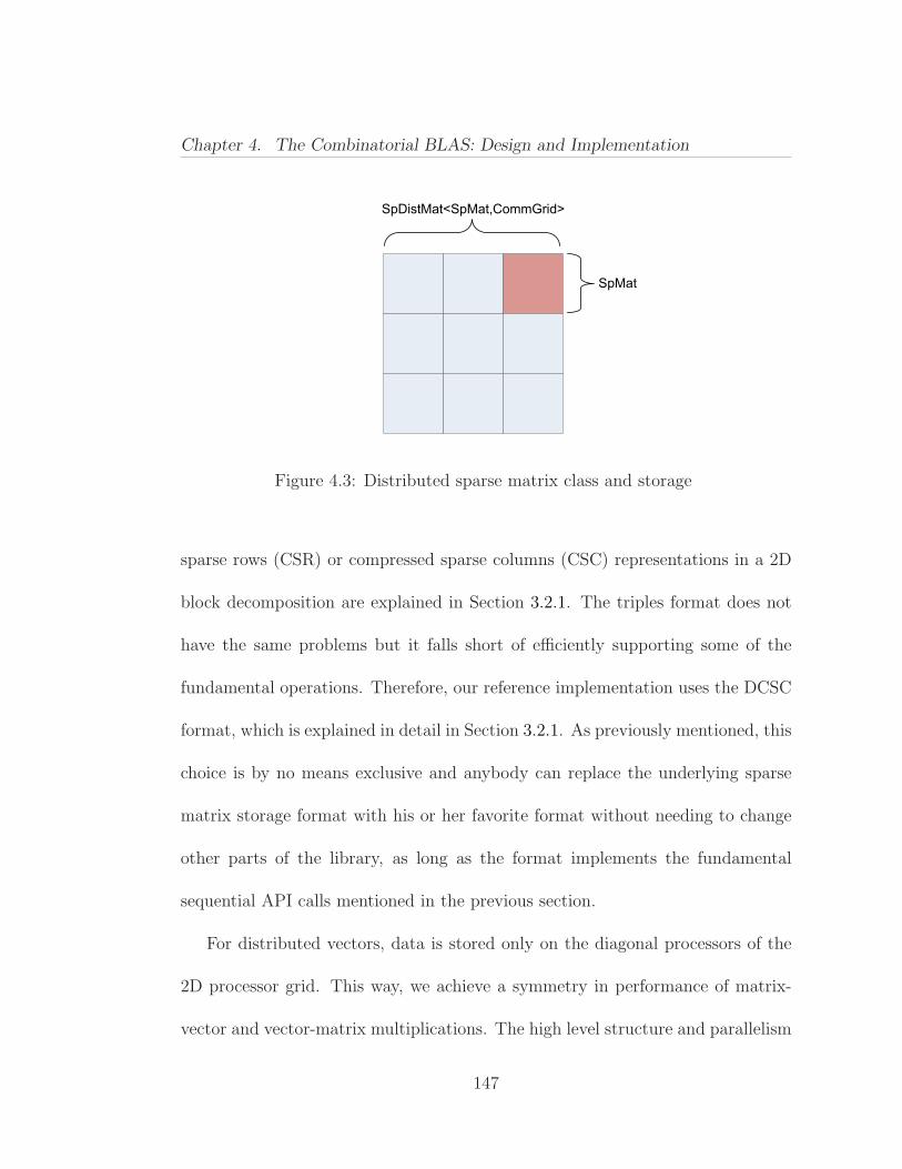
Chapter 4. The Combinatorial BLAS: Design and Implementation
SpDistMat<SpMat,CommGrid>
SpMat
Figure 4.3: Distributed sparse matrix class and storage
sparse rows (CSR) or compressed sparse columns (CSC) representations in a 2D
block decomposition are explained in Section 3.2.1. The triples format does not
have the same problems but it falls short of efficiently supporting some of the
fundamental operations. Therefore, our reference implementation uses the DCSC
format, which is explained in detail in Section 3.2.1. As previously mentioned, this
choice is by no means exclusive and anybody can replace the underlying sparse
matrix storage format with his or her favorite format without needing to change
other parts of the library, as long as the format implements the fundamental
sequential API calls mentioned in the previous section.
For distributed vectors, data is stored only on the diagonal processors of the
2D processor grid. This way, we achieve a symmetry in performance of matrix-
vector and vector-matrix multiplications. The high level structure and parallelism
147
Chapter 4. The Combinatorial BLAS: Design and Implementation
of sparse and dense vectors are the same, the only difference being how the local
data is stored in processors. A dense vector naturally uses a dense array, while a
sparse vector is internally represented as a list of index-value pairs.
148
Chapter 5
The Combinatorial BLAS:Applications and PerformanceAnalysis
The joy of life consists in the exercise of one’s energies, continualgrowth, constant change, the enjoyment of every new experience. Tostop means simply to die. The eternal mistake of mankind is to set upan attainable ideal.
Aleister Crowley (1875-1947)
This chapter presents two applications of the Combinatorial BLAS library.
We report the performance of two algorithms on distributed-memory clusters,
implemented using the Combinatorial BLAS primitives. The code for these appli-
cations, along with an alpha release of the complete library, can be freely obtained
from http://gauss.cs.ucsb.edu/code/index.shtml.
149

Chapter 5. The Combinatorial BLAS: Applications and Performance Analysis
5.1 Betweenness Centrality
Betweenness centrality [96], a centrality metric based on shortest paths, is
the main computation on which we evaluate the performance of our proof-of-
concept implementation of the Combinatorial BLAS. There are two reasons for
this choice. Firstly, it is a widely-accepted metric that is used to quantify the
relative importance of vertices in the graph. Betweenness centrality (BC) of a
vertex captures the normalized ratio of the number of shortest paths that pass
through a vertex to the total number of shortest paths in the graph. This is
formalized in Equation 5.1 where σst denote the number of shortest paths from s
to t, and σst(v) is the number of such paths passing through vertex v.
BC(v) =∑
s 6=v 6=t∈V
σst(v)
σst
(5.1)
A vertex v with a high betweenness centrality is therefore an important one
based on at least two different interpretations. From the point of view of other
vertices, it is a highly sought-after hop for reaching others as quickly as possible.
The second possible interpretation is that v itself is the best-situated vertex to
reach others as quickly as possible.
The second reason for presenting the betweenness centrality as a success metric
is its quantifiability. It is part of the HPC Scalable Graph Analysis Benchmarks
150
Chapter 5. The Combinatorial BLAS: Applications and Performance Analysis
(formerly known as the HPCS Scalable Synthetic Compact Applications #2 [16])
and various implementations on different platforms exist [18, 144, 190] for com-
parison.
We compute betweenness centrality using Brandes’ algorithm [40]. It computes
single source shortest paths from each node in the network and increases the
respective BC score for nodes on the path. The algorithm requires O(nm) time
for unweighted graphs and O(nm + n2 log n) time for weighted graphs, where n
is the number of nodes and m is the number of edges in the graph. The sizes
of real-world graphs are prohibitive for exact calculation, so we resort to efficient
approximations. An unbiased estimator of the betweenness centrality score has
been proposed based on sampling nodes from which to compute single-source
shortest paths [19]. The resulting scores approximate a uniformly scaled version
of the actual betweenness centrality score. We only focus on unweighted graphs
in this performance study.
Following the specification of the graph analysis benchmark [16], we used R-
MAT matrices as inputs. Due to the prohibitive cost of the exact algorithm,
we used the approximate algorithm with 8192 starting vertices. We measure the
performance using the Traversed Edges Per Second (TEPS) rate, which is an
algorithmic performance count that is independent of the particular implemen-
tation [16]. We randomly relabeled the vertices in the generated graph, before
151
Chapter 5. The Combinatorial BLAS: Applications and Performance Analysis
storing it for subsequent runs. For reproducibility of results, we chose starting
vertices using a deterministic process, specifically excluding disconnected vertices
as starting vertices (which would have boosted the TEPS scores artificially).
We implemented an array-based formulation of the Brandes’ algorithm, due
to Robinson and Kepner. A reference Matlab implementation is publicly avail-
able from the Graph Analysis webpage [17]. The workhorse of the algorithm is
a parallel breadth-first search that is performed from multiple source vertices.
In Combinatorial BLAS, one step of the breadth-first search is implemented as
the multiplication of the transpose of the adjacency matrix of the graph with a
rectangular matrix X where the ith column of X represents the current frontier
of the ith independent breadth-first search tree. Inially, each column of X has
only one nonzero that represents the starting vertex of the breadth-first search,
i.e. X(:, i) = ej where vertex j is the i-th starting vertex for the current iteration.
Similarly, the tallying step is also implemented as an SpGEMM operation.
For the performance results presented in this section, we use a synchronous im-
plementaton of the Sparse SUMMA algorithm described in Section 3.3.5, because
it is the most portable SpGEMM implementation that relies only on simple MPI-1
features. The other Combinatorial BLAS primitives that are used for implement-
ing the betweenness centrality algorithm are reductions along one dimension and
elementwise operations for sparse/sparse, sparse/dense, and dense/sparse input
152
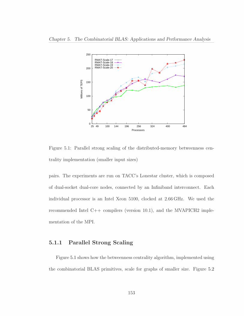
Chapter 5. The Combinatorial BLAS: Applications and Performance Analysis
0
50
100
150
200
250
25 49 100 144 196 256 324 400 484
Mill
ions
of T
EP
S
Processors
RMAT-Scale-17RMAT-Scale-18RMAT-Scale-19RMAT-Scale-20
Figure 5.1: Parallel strong scaling of the distributed-memory betweenness cen-
trality implementation (smaller input sizes)
pairs. The experiments are run on TACC’s Lonestar cluster, which is composed
of dual-socket dual-core nodes, connected by an Infiniband interconnect. Each
individual processor is an Intel Xeon 5100, clocked at 2.66 GHz. We used the
recommended Intel C++ compilers (version 10.1), and the MVAPICH2 imple-
mentation of the MPI.
5.1.1 Parallel Strong Scaling
Figure 5.1 shows how the betweenness centrality algorithm, implemented using
the combinatorial BLAS primitives, scale for graphs of smaller size. Figure 5.2
153
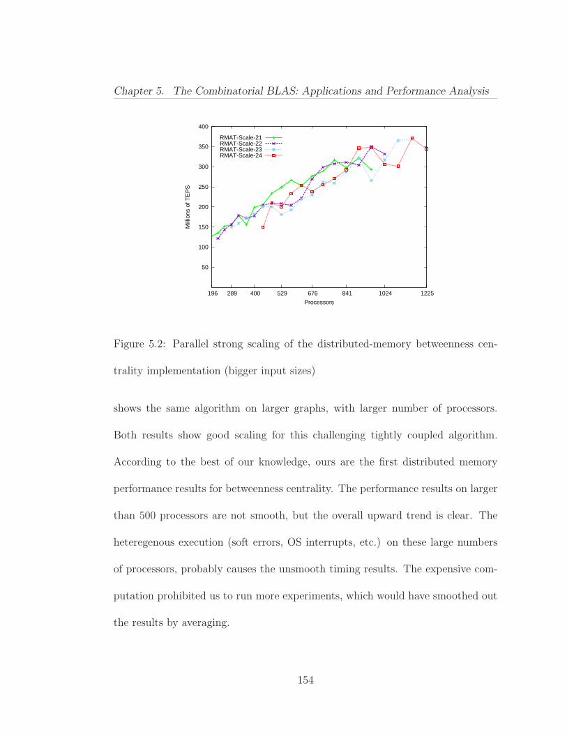
Chapter 5. The Combinatorial BLAS: Applications and Performance Analysis
50
100
150
200
250
300
350
400
196 289 400 529 676 841 1024 1225
Mill
ions
of T
EP
S
Processors
RMAT-Scale-21RMAT-Scale-22RMAT-Scale-23RMAT-Scale-24
Figure 5.2: Parallel strong scaling of the distributed-memory betweenness cen-
trality implementation (bigger input sizes)
shows the same algorithm on larger graphs, with larger number of processors.
Both results show good scaling for this challenging tightly coupled algorithm.
According to the best of our knowledge, ours are the first distributed memory
performance results for betweenness centrality. The performance results on larger
than 500 processors are not smooth, but the overall upward trend is clear. The
heteregenous execution (soft errors, OS interrupts, etc.) on these large numbers
of processors, probably causes the unsmooth timing results. The expensive com-
putation prohibited us to run more experiments, which would have smoothed out
the results by averaging.
154
Chapter 5. The Combinatorial BLAS: Applications and Performance Analysis
The best performance results for this problem is due to Madduri et al. [144] us-
ing an optimized implementation specifically tailored for massively multithreaded
architectures. They report a maximum of 160 million TEPS for an R-MAT graph
of scale 24 on the 16-processor XMT machine. On the MTA-2 machine, which is
the predecessor to the XMT, the same optimized code achieved 353 million TEPS
on 40 processors. Our code, on the other hand, is truely generic and contains no
problem and machine specific optimizations. We did not even attempt to opti-
mize our primitives for the skewed aspect ratio (ratio of dimensions) of most of
the matrices involved. For this problem instance, 900 processors of Lonestar was
equivalent to 40 processors of MTA-2. The cost and power efficiency comparisons
of these two solutions does not exist yet.
5.1.2 Sensitivity to Batch Processing
As mentioned earlier, most of the parallelism comes from the coarse-grained
SpGEMM operation that is used to perform breadth-first searches from multiple
source vertices. By changing the batchsize, the number of source vertices that
are processed together, we obtain a trade-off between space usage and potential
parallelism. The space increases linearly with increasing batchsize. As we show
experimentally, the performance also increases substantially, especially for large
number of processors. In Figure 5.3, we show the strong scaling of our betweenness
155
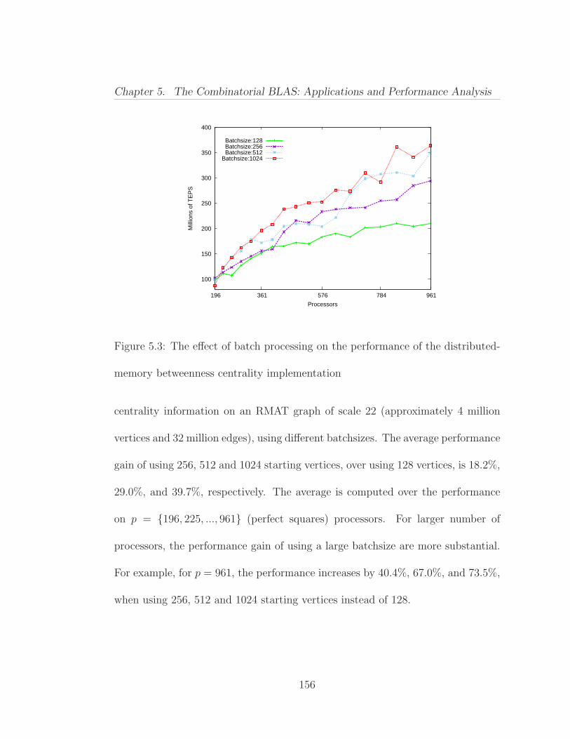
Chapter 5. The Combinatorial BLAS: Applications and Performance Analysis
100
150
200
250
300
350
400
196 361 576 784 961
Mill
ions
of T
EP
S
Processors
Batchsize:128Batchsize:256Batchsize:512
Batchsize:1024
Figure 5.3: The effect of batch processing on the performance of the distributed-
memory betweenness centrality implementation
centrality information on an RMAT graph of scale 22 (approximately 4 million
vertices and 32 million edges), using different batchsizes. The average performance
gain of using 256, 512 and 1024 starting vertices, over using 128 vertices, is 18.2%,
29.0%, and 39.7%, respectively. The average is computed over the performance
on p = 196, 225, ..., 961 (perfect squares) processors. For larger number of
processors, the performance gain of using a large batchsize are more substantial.
For example, for p = 961, the performance increases by 40.4%, 67.0%, and 73.5%,
when using 256, 512 and 1024 starting vertices instead of 128.
156
Chapter 5. The Combinatorial BLAS: Applications and Performance Analysis
5.2 Markov Clustering
Markov clustering (MCL) algorithm [82] is a flow based graph clustering al-
gorithm that has been extremely popular in computational biology, among other
fields. It simulates a Markov process to the point where clusters can be identified
by simple interpretation of the modified adjacency matrix of the graph. Compu-
tationally, it alternates between an expansion step where the adjacency matrix
is raised to its nth power (typically n = 2, so it is practically a squaring opera-
tion), and an inflation step where in every column of the adjacency matrix, the
scalar entries are raised to the dth power (d > 1) and renormalized within the
column. Inflation operation boosts the larger entries and effectively sends the
smaller entries to close to zero. MCL achieves scalability and storage efficiency
by maintaining sparsity of its matrix. This is done by pruning up close to zero
entries after the inflation.
Implementing the MCL algorithm using the Combinatorial BLAS primitives
generates a very concise code that feels natural. Full MCL code, except for the
interpretation part, is shown in Figure 5.5, while the inflation subroutine is shown
in Figure 5.4.
Van Dongen [202] provides a fast sequential implementation of the MCL al-
gorithm. We do not attempt an apples-to-apples comparison with the original
157
Chapter 5. The Combinatorial BLAS: Applications and Performance Analysis
template <typename IT , typename NT, typename DER>void I n f l a t e (SpParMat<IT ,NT,DER> & A, double power )
A. Apply ( bind2nd ( exponent ia te ( ) , power ) ) ;
/* reduce to Row, columns are c o l l a p s e d to s i n g l e e n t r i e s */DenseParVec<IT ,NT> colsums = Reduce (Row, plus<NT>() , 0 . 0 ) ;
colsums . Apply ( b ind1st ( d iv ide s <double>() , 1 ) ) ;
/* s c a l e each Column with the g iven row vec to r */A. DimScale ( colsums , Column ) ;
Figure 5.4: Inflation code using the Combinatorial BLAS primitives
int main ( )
SpParMat<unsigned , double , SpDCCols<unsigned , double> > A;A. ReadDistr ibute ( ‘ ‘ inputmatr ix ’ ’ ) ;
o ldchaos = Chaos (A) ;newchaos = oldchaos ;
// wh i l e t h e r e i s an ep s i l o n improvementwhile ( ( o ldchaos − newchaos ) > EPS)
A. Square ( ) ; // expandI n f l a t e (A, 2 ) ; // i n f l a t e ( and renormal i ze )A. Prune ( bind2nd ( l e s s <double>() , 0 . 0 0 0 1 ) ) ;o ldchaos = newchaos ;newchaos = Chaos (A) ;
I n t e r p r e t (A) ;
Figure 5.5: MCL code using the Combinatorial BLAS primitives
158
Chapter 5. The Combinatorial BLAS: Applications and Performance Analysis
implementation, as the official mcl software has many options, something we can
not replicate in our 10-15 lines prototype. The sequential mcl code is twice as
fast as our parallel implementation running on a single processor. This is mostly
due to its finer control over sparsity parameters, such as limiting the number of
nonzeros in each row/column. Serial performance is not a bottleneck, as our code
achieves superlinear speedup until p = 1024.
Figure 5.6 shows the speedup of the three most expensive iterations, that
together make up more than 99% of the total running time. The input is a
permuted R-MAT graph of scale 14, with self loops added for convergence. On
4096 processors, we were able to cluster this graph in less than a second. The
same graph takes more than half an hour to cluster on a single processor. Note
that iteration #4 takes only 70 milliseconds using 1024 processors, which is hard
to scale further due to parallelization overheads on thousands of processors. We
were able to cluster gigascale graphs using our implementation of MCL using
the Combinatorial BLAS. We report on a smaller instance in order to provide a
complete strong scaling result.
159
Chapter 5. The Combinatorial BLAS: Applications and Performance Analysis
0
500
1000
1500
2000
2500
3000
3500
4000
0 500 1000 1500 2000 2500 3000 3500 4000 4500
Spe
edup
Processors
Iteration #2Iteration #3Iteration #4
Figure 5.6: Strong scaling of the three most expensive iterations while clustering
an R-MAT graph of scale 14 using the MCL algorithm implemented using the
Combinatorial BLAS
160

Chapter 6
Parallel Sparse y ← Ax andy ← ATx Using Compressed SparseBlocks
Abstract
This chapter introduces a storage format for sparse matrices, calledcompressed sparse blocks (CSB), which allows both Ax and ATxto be computed efficiently in parallel, where A is an n×n sparse matrixwith nnz ≥ n nonzeros and x is a dense n-vector. Our algorithmsuse Θ(nnz ) work (serial running time) and Θ(
√n lg n) span (critical-
path length), yielding a parallelism of Θ(nnz /√
n lg n), which is amplyhigh for virtually any large matrix. The storage requirement for CSB isesssentially the same as that for the more-standard compressed-sparse-rows (CSR) format, for which computing Ax in parallel is easy but ATxis difficult. Benchmark results indicate that on one processor, the CSBalgorithms for Ax and ATx run just as fast as the CSR algorithm forAx, but the CSB algorithms also scale up linearly with processors untillimited by off-chip memory bandwidth.
161

Chapter 6. Parallel Sparse y ← Ax and y ← ATx Using Compressed Sparse
Blocks
This chapter is based on a paper [47] by Buluc et al. from SPAA 2009. The
indices are zero based, different from the rest of the thesis.
6.1 Introduction
When multiplying a large n × n sparse matrix A having nnz nonzeros by a
dense n-vector x, the memory bandwidth for reading A can limit overall perfor-
mance. Consequently, most algorithms to compute Ax store A in a compressed
format. One simple “tuple” representation stores each nonzero of A as a triple
consisting of its row index, its column index, and the nonzero value itself. This
representation, however, requires storing 2nnz row and column indices, in addi-
tion to the nonzeros. The current standard storage format for sparse matrices in
scientific computing, compressed sparse rows (CSR) [171], is more efficient,
because it stores only n+nnz indices or pointers. This reduction in storage of CSR
compared with the tuple representation tends to result in faster serial algorithms.
In the domain of parallel algorithms, however, CSR has its limitations. Al-
though CSR lends itself to a simple parallel algorithm for computing the matrix-
vector product Ax, this storage format does not admit an efficient parallel algo-
rithm for computing the product ATx, where AT denotes the transpose of the
matrix A — or equivalently, for computing the product xTA of a row vector
162

Chapter 6. Parallel Sparse y ← Ax and y ← ATx Using Compressed Sparse
Blocks
xT by A. Although one could use compressed sparse columns (CSC) to
compute ATx, many applications, including iterative linear system solvers such
as biconjugate gradients and quasi-minimal residual [171], require both Ax and
ATx. One could transpose A explicitly, but computing the transpose for either
CSR or CSC formats is expensive. Moreover, since matrix-vector multiplication
for sparse matrices is generally limited by memory bandwidth, it is desirable to
find a storage format for which both Ax and ATx can be computed in paral-
lel without performing more than nnz fetches of nonzeros from the memory to
compute either product.
This paper presents a new storage format called compressed sparse blocks
(CSB) for representing sparse matrices. Like CSR and CSC, the CSB format
requires only n+nnz words of storage for indices. Because CSB does not favor rows
over columns or vice versa, it admits efficient parallel algorithms for computing
either Ax or ATx, as well as for computing Ax when A is symmetric and only half
the matrix is actually stored.
Previous work on parallel sparse matrix-vector multiplication has focused on
reducing communication volume in a distributed-memory setting, often by using
graph or hypergraph partitioning techniques to find good data distributions for
particular matrices ([54, 203], for example). Good partitions generally exist for
matrices whose structures arise from numerical discretizations of partial differen-
163

Chapter 6. Parallel Sparse y ← Ax and y ← ATx Using Compressed Sparse
Blocks
0
100
200
300
400
500
1 2 3 4 5 6 7 8
MF
lops
/sec
Processors
CSB_SpMVCSB_SpMV_T
CSR_SpMV(Serial)CSR_SpMV_T(Serial)
Star-P(y=Ax)Star-P(y’=x’A)
Figure 6.1: Average performance of Ax and ATx operations on 13 different ma-
trices from our benchmark test suite. CSB SpMV and CSB SpMV T use com-
pressed sparse blocks to perform Ax and ATx, respectively. CSR SpMV (Serial)
and CSR SpMV T (Serial) use OSKI [205] and compressed sparse rows without
any matrix-specific optimizations. Star-P (y=Ax) and Star-P (y’=x’A) use Star-
P [179], a parallel code based on CSR. The experiments were run on a ccNUMA
architecture powered by AMD Opteron 8214 (Santa Rosa) processors.
tial equations in two or three spatial dimensions. Our work, by contrast, is moti-
vated by multicore and manycore architectures, in which parallelism and memory
bandwidth are key resources. Our algorithms are efficient in these measures for
matrices with arbitrary nonzero structure.
Figure 6.1 presents an overall summary of achieved performance. The serial
CSR implementation uses plain OSKI [205] without any matrix-specific optimiza-
164
Chapter 6. Parallel Sparse y ← Ax and y ← ATx Using Compressed Sparse
Blocks
tions. The graph shows the average performance over all our test matrices except
for the largest, which failed to run on Star-P [179] due to memory constraints.
The performance is measured in Mflops (Millions of FLoating-point OPerationS)
per second. Both Ax and ATx take 2 nnz flops. To measure performance, we di-
vide this value by the time it takes for the computation to complete. Section 6.7
provides detailed performance results.
The remainder of this paper is organized as follows. Section 6.2 discusses the
limitations of the CSR/CSC formats for parallelizing Ax and ATx calculations.
Section 6.3 describes the CSB format for sparse matrices. Section 6.4 presents
the algorithms for computing Ax and ATx using the CSB format, and Section 6.5
provides a theoretical analysis of their parallel performance. Section 6.6 describes
the experimental setup we used, and Section 6.7 presents the results. Section 6.8
offers some concluding remarks.
6.2 Conventional storage formats
This section describes the CSR and CSC sparse-matrix storage formats and
explores their limitations when it comes to computing both Ax and ATx in parallel.
We review the work/span formulation of parallelism and show that performing Ax
with CSR (or equivalently ATx with CSC) yields ample parallelism. We consider
165
Chapter 6. Parallel Sparse y ← Ax and y ← ATx Using Compressed Sparse
Blocks
various strategies for performing ATx in parallel with CSR (or equivalently Ax
with CSC) and why they are problematic.
The compressed sparse row (CSR) format stores the nonzeros (and ideally
only the nonzeros) of each matrix row in consecutive memory locations, and it
stores an index to the first stored element of each row. In one popular variant
[77], CSR maintains one floating-point array val [nnz ] and two integer arrays,
col ind [nnz ] and row ptr [n] to store the matrix A = (aij). The row ptr array
stores the index of each row in val . That is, if val [k] stores matrix element aij,
then row ptr [i] ≤ k < row ptr [i+1]. The col ind array stores the column indices
of the elements in the val array. That is, if val [k] stores matrix element aij, then
col ind [k] = j.
The compressed sparse column (CSC) format is analogous to CSR, except that
the nonzeros of each column, instead of row, are stored in contiguous memory
locations. In other words, the CSC format for A is obtained by storing AT in
CSR format.
The earliest written description of CSR that we have been able to divine from
the literature is an unnamed “scheme” presented in Table 1 of the 1967 article [195]
by Tinney and Walker, although in 1963 Sato and Tinney [175] allude to what is
probably CSR. Markowitz’s seminal paper [148] on sparse Gaussian elimination
does not discuss data structures, but it is likely that Markowitz used such a
166
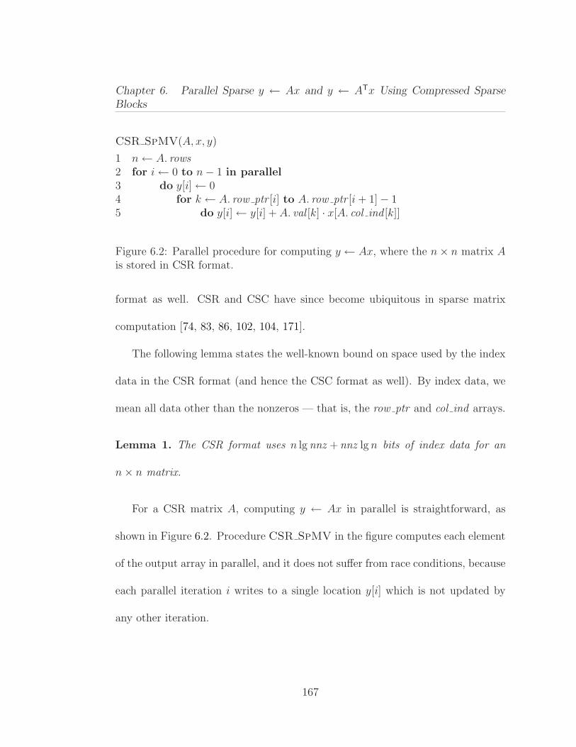
Chapter 6. Parallel Sparse y ← Ax and y ← ATx Using Compressed Sparse
Blocks
CSR SpMV(A, x, y)
1 n← A. rows2 for i← 0 to n− 1 in parallel3 do y[i]← 04 for k ← A. row ptr [i] to A. row ptr [i + 1]− 15 do y[i]← y[i] + A. val [k] · x[A. col ind [k]]
Figure 6.2: Parallel procedure for computing y ← Ax, where the n× n matrix Ais stored in CSR format.
format as well. CSR and CSC have since become ubiquitous in sparse matrix
computation [74, 83, 86, 102, 104, 171].
The following lemma states the well-known bound on space used by the index
data in the CSR format (and hence the CSC format as well). By index data, we
mean all data other than the nonzeros — that is, the row ptr and col ind arrays.
Lemma 1. The CSR format uses n lg nnz + nnz lg n bits of index data for an
n× n matrix.
For a CSR matrix A, computing y ← Ax in parallel is straightforward, as
shown in Figure 6.2. Procedure CSR SpMV in the figure computes each element
of the output array in parallel, and it does not suffer from race conditions, because
each parallel iteration i writes to a single location y[i] which is not updated by
any other iteration.
167

Chapter 6. Parallel Sparse y ← Ax and y ← ATx Using Compressed Sparse
Blocks
We shall measure the complexity of this code, and other codes in this paper,
in terms of work and span [69, Ch. 27]:
• The work , denoted by T1, is the running time on 1 processor.
• The span ,1 denoted by T∞, is running time on an infinite number of pro-
cessors.
The parallelism of the algorithm is T1/T∞, which corresponds to the maximum
possible speedup on any number of processors. Generally, if a machine has some-
what fewer processors than the parallelism of an application, a good scheduler
should be able to achieve linear speedup. Thus, for a fixed amount of work, our
goal is to achieve a sufficiently small span so that the parallelism exceeds the
number of processors by a reasonable margin.
The work of CSR SpMV is Θ(nnz ), assuming, as we shall, that nnz ≥ n,
because the body of the outer loop starting in line 2 executes for n iterations, and
the body of the inner loop starting in line 4 executes for the number of nonzeros
in the ith row, for a total of nnz times.
The span of CSR SpMV depends on the maximum number nr of nonzeros
in any row of the matrix A, since that number determines the worst-case time of
any iteration of the loop in line 4. The n iterations of the parallel loop in line 2
1The literature also uses the terms depth [34] and critical-path length [35].
168
Chapter 6. Parallel Sparse y ← Ax and y ← ATx Using Compressed Sparse
Blocks
contribute Θ(lg n) to the span, assuming that loops are implemented as binary
recursion. Thus, the total span is Θ(nr + lg n).
The parallelism is therefore Θ(nnz /(nr + lg n)). In many common situations,
we have nnz = Θ(n), which we will assume for estimation purposes. The maxi-
mum number nr of nonzeros in any row can vary considerably, however, from a
constant, if all rows have an average number of nonzeros, to n, if the matrix has a
dense row. If nr = O(1), then the parallelism is Θ(nnz / lg n), which is quite high
for a matrix with a billion nonzeros. In particular, if we ignore constants for the
purpose of making a ballpark estimate, we have nnz / lg n ≈ 109/(lg 109) > 3×10⁷,
which is much larger than any number of processors one is likely to encounter in
the near future. If nr = Θ(n), however, as is the case when there is even a
single dense row, we have parallelism Θ(nnz /n) = Θ(1), which limits scalability
dramatically. Fortunately, we can parallelize the inner loop (line 4) using divide-
and-conquer recursion to compute the sparse inner product in lg(nr) span without
affecting the asymptotic work, thereby achieving parallelism Θ(nnz / lg n) in all
cases.
Computing ATx serially can be accomplished by simply interchanging the row
and column indices [79], yielding the pseudocode shown in Figure 6.3. The work
of procedure CSR SpMV T is Θ(nnz ), the same as CSR SpMV.
169

Chapter 6. Parallel Sparse y ← Ax and y ← ATx Using Compressed Sparse
Blocks
CSR SpMV T(A, x, y)
1 n← A. cols2 for i← 0 to n− 13 do y[i]← 04 for i← 0 to n− 15 do for k ← A. row ptr [i] to A. row ptr [i + 1]− 16 do y[A. col ind [k]]← y[A. col ind [k]] + A. val [k] · x[i]
Figure 6.3: Serial procedure for computing y ← ATx, where the n × n matrix Ais stored in CSR format.
Parallelizing CSR SpMV T is not straightforward, however. We shall review
several strategies to see why it is problematic.
One idea is to parallelize the loops in lines 2 and 5, but this strategy yields
minimal scalability. First, the span of the procedure is Θ(n), due to the loop in
line 4. Thus, the parallelism can be at most O(nnz /n), which is a small constant
in most common situations. Second, in any practical system, the communication
and synchronization overhead for executing a small loop in parallel is much larger
than the execution time of the few operations executed in line 6.
Another idea is to execute the loop in line 4 in parallel. Unfortunately, this
strategy introduces race conditions in the read/modify/write to y[A. col ind [k]] in
line 6.2 These races can be addressed in two ways, neither of which is satisfactory.
2In fact, if nnz > n, then the “pigeonhole principle” guarantees that the program has at leastone race condition.
170

Chapter 6. Parallel Sparse y ← Ax and y ← ATx Using Compressed Sparse
Blocks
The first solution involves locking column col ind [k] or using some other form
of atomic update.3 This solution is unsatisfactory because of the high overhead
of the lock compared to the cost of the update. Moreover, if A contains a dense
column, then the contention on the lock is Θ(n), which completely destroys any
parallelism in the common case where nnz = Θ(n).
The second solution involves splitting the output array y into multiple arrays
yp in a way that avoids races, and then accumulating y ← Σpyp at the end of the
computation. For example, in a system with P processors (or threads), one could
postulate that processor p only operates on array yp, thereby avoiding any races.
This solution is unsatisfactory because the work becomes Θ(nnz +Pn), where the
last term comes from the need to initialize and accumulate P (dense) length-n
arrays. Thus, the parallel execution time is Θ((nnz +Pn)/P ) = Ω(n) no matter
how many processors are available.
A third idea for parallelizing ATx is to compute the transpose explicitly and
then use CSR SpMV. Unfortunately, parallel transposition of a sparse matrix in
CSR format is costly and encounters exactly the same problems we are trying to
avoid. Moreover, every element is accessed at least twice: once for the transpose,
and once for the multiplication. Since the calculation of a matrix-vector product
3No mainstream hardware supports atomic update of floating-point quantities, however.
171
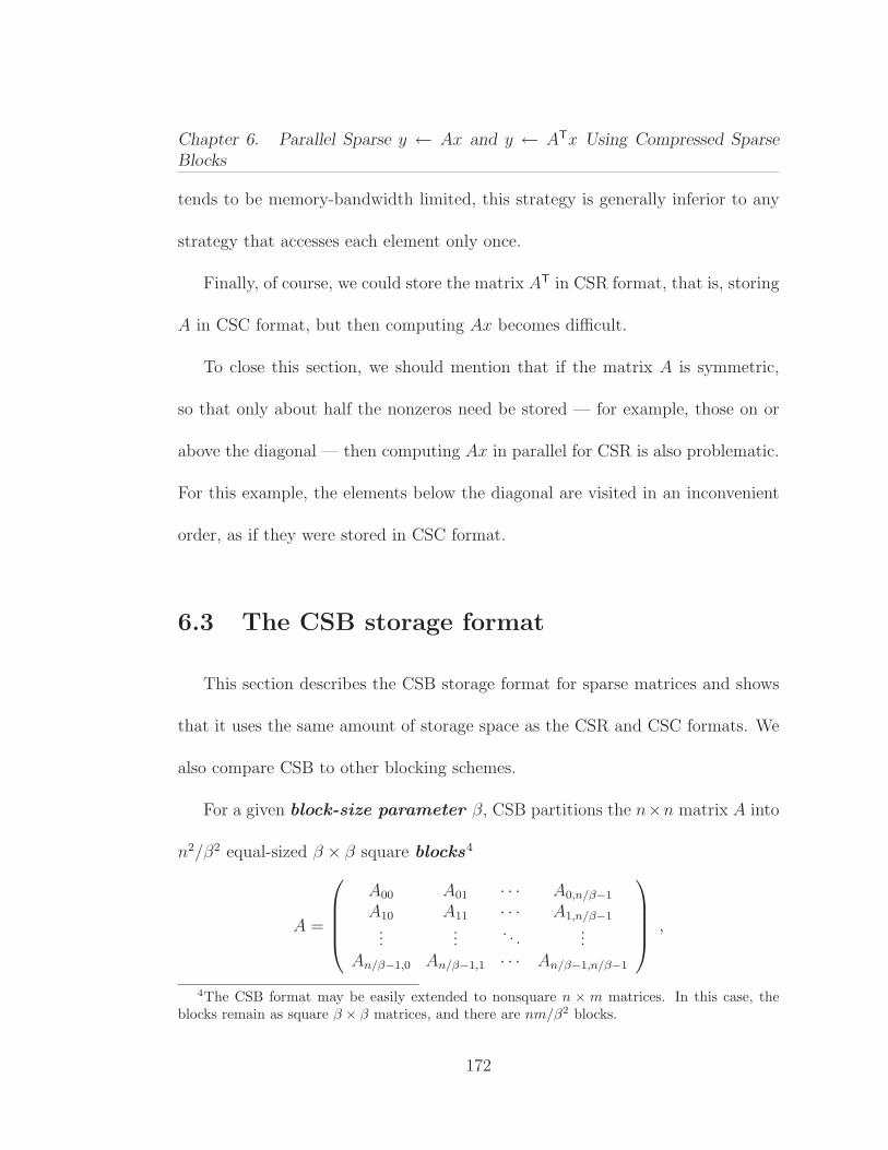
Chapter 6. Parallel Sparse y ← Ax and y ← ATx Using Compressed Sparse
Blocks
tends to be memory-bandwidth limited, this strategy is generally inferior to any
strategy that accesses each element only once.
Finally, of course, we could store the matrix AT in CSR format, that is, storing
A in CSC format, but then computing Ax becomes difficult.
To close this section, we should mention that if the matrix A is symmetric,
so that only about half the nonzeros need be stored — for example, those on or
above the diagonal — then computing Ax in parallel for CSR is also problematic.
For this example, the elements below the diagonal are visited in an inconvenient
order, as if they were stored in CSC format.
6.3 The CSB storage format
This section describes the CSB storage format for sparse matrices and shows
that it uses the same amount of storage space as the CSR and CSC formats. We
also compare CSB to other blocking schemes.
For a given block-size parameter β, CSB partitions the n×n matrix A into
n2/β2 equal-sized β × β square blocks4
A =
A00 A01 · · · A0,n/β−1
A10 A11 · · · A1,n/β−1...
.... . .
...An/β−1,0 An/β−1,1 · · · An/β−1,n/β−1
,
4The CSB format may be easily extended to nonsquare n × m matrices. In this case, theblocks remain as square β × β matrices, and there are nm/β2 blocks.
172
Chapter 6. Parallel Sparse y ← Ax and y ← ATx Using Compressed Sparse
Blocks
where the block Aij is the β × β submatrix of A containing elements falling in
rows iβ, iβ +1, . . . , (i+1)β− 1 and columns jβ, jβ +1, . . . , (j +1)β− 1 of A. For
simplicity of presentation, we shall assume that β is an exact power of 2 and that
it divides n; relaxing these assumptions is straightforward.
Many or most of the individual blocks Aij are hypersparse [49], meaning
that the ratio of nonzeros to matrix dimension is asymptotically 0. For example,
if β =√
n and nnz = cn, the average block has dimension√
n and only c nonzeros.
The space to store a block should therefore depend only on its nonzero count, not
on its dimension.
CSB represents a block Aij by compactly storing a triple for each nonzero,
associating with the nonzero data element a row and column index. In contrast
to the column index stored for each nonzero in CSR, the row and column indices lie
within the submatrix Aij, and hence require fewer bits. In particular, if β =√
n,
then each index into Aij requires only half the bits of an index into A. Since these
blocks are stored contiguously in memory, CSB uses an auxiliary array of pointers
to locate the beginning of each block.
More specifically, CSB maintains a floating-point array val [nnz ], and three
integer arrays row ind [nnz], col ind [nnz ], and blk ptr [n2/β2]. We describe each
of these arrays in turn.
173

Chapter 6. Parallel Sparse y ← Ax and y ← ATx Using Compressed Sparse
Blocks
The val array stores all the nonzeros of the matrix and is analogous to CSR’s
array of the same name. The difference is that CSR stores rows contiguously,
whereas CSB stores blocks contiguously. Although each block must be contiguous,
the ordering among blocks is flexible. Let f(i, j) be the bijection from pairs of
block indices to integers in the range 0, 1, . . . , n2/β2−1 that describes the ordering
among blocks. That is, f(i, j) < f(i′, j′) if and only if Aij appears before Ai′j′ in
val . We discuss choices of ordering later in this section.
The row ind and col ind arrays store the row and column indices, respectively,
of the elements in the val array. These indices are relative to the block containing
the particular element, not the entire matrix, and hence they range from 0 to
β − 1. That is, if val [k] stores the matrix element aiβ+r,jβ+c, which is located in
the rth row and cth column of the block Aij, then row ind = r and col ind = c.
As a practical matter, we can pack a corresponding pair of elements of row ind
and col ind into a single integer word of 2 lg β bits so that they make a single
array of length nnz , which is comparable to the storage needed by CSR for the
col ind array.
The blk ptr array stores the index of each block in the val array, which is
analogous to the row ptr array for CSR. If val [k] stores a matrix element falling
in block Aij, then blk ptr [f(i, j)] ≤ k < blk ptr [f(i, j) + 1].
The following lemma states the storage used for indices in the CSB format.
174
Chapter 6. Parallel Sparse y ← Ax and y ← ATx Using Compressed Sparse
Blocks
Lemma 2. The CSB format uses (n2/β2) lg nnz +2 nnz lg β bits of index data.
Proof. Since the val array contains nnz elements, referencing an element requires
lg nnz bits, and hence the blk ptr array uses (n2/β2) lg nnz bits of storage.
For each element in val , we use lg β bits to represent the row index and lg β bits
to represent the column index, requiring a total of nnz lg β bits for each of row ind
and col ind . Adding the space used by all three indexing arrays completes the
proof.
To better understand the storage requirements of CSB, we present the follow-
ing corollary for β =√
n. In this case, both CSR (Lemma 1) and CSB use the
same storage.
Corollary 3. The CSB format uses n lg nnz + nnz lg n bits of index data when
β =√
n.
Thus far, we have not addressed the ordering of elements within each block or
the ordering of blocks. Within a block, we use a Z-Morton ordering [151], storing
first all those elements in the top-left quadrant, then the top-right, bottom-left,
and finally bottom-right quadrants, using the same layout recursively within each
quadrant. In fact, these quadrants may be stored in any order, but the recursive
ordering is necessary for our algorithm to achieve good parallelism within a block.
175
Chapter 6. Parallel Sparse y ← Ax and y ← ATx Using Compressed Sparse
Blocks
The choice of storing the nonzeros within blocks in a recursive layout is op-
posite to the common wisdom for storing dense matrices [87]. Although most
compilers and architectures favor conventional row/column ordering for optimal
prefetching, the choice of layout within the block becomes less significant for sparse
blocks as they already do not take full advantage of such features. More impor-
tantly, a recursive ordering allows us to efficiently determine the four quadrants
of a block using binary search, which is crucial for parallelizing individual blocks.
Our algorithm and analysis do not, however, require any particular ordering
among blocks. A Z-Morton ordering (or any recursive ordering) seems desirable
as it should get better performance in practice by providing spatial locality, and
it matches the ordering within a block. Computing the function f(i, j), however,
is simpler for a row-major or column-major ordering among blocks.
Comparison with other blocking methods
A blocked variant of CSR, called BCSR, has been used for improving register
reuse [122]. In BCSR, the sparse matrix is divided into small dense blocks that
are stored in consecutive memory locations. The pointers are maintained to the
first block on each row of blocks. BCSR storage is converse to CSB storage,
because BCSR stores a sparse collection of dense blocks, whereas CSB stores a
176
Chapter 6. Parallel Sparse y ← Ax and y ← ATx Using Compressed Sparse
Blocks
dense collection of sparse blocks. We conjecture that it would be advantageous to
apply BCSR-style register blocking to each individual sparse block of CSB.
Nishtala et al. [154] have proposed a data structure similar to CSB in the
context of cache blocking. Our work differs from theirs in two ways. First, CSB
is symmetric without favoring rows over columns. Second, our algorithms and
analysis for CSB are designed for parallelism instead of cache performance. As
shown in Section 6.5, CSB supports ample parallelism for algorithms computing
Ax and ATx, even on sparse and irregular matrices.
Blocking is also used in dense matrices. The Morton-hybrid layout [5, 142], for
example, uses a parameter equivalent to our parameter β for selecting the block
size. Whereas in CSB we store elements in a Morton ordering within blocks and
an arbitrary ordering among blocks, the Morton-hybrid layout stores elements
in row-major order within blocks and a Morton ordering among blocks. The
Morton-hybrid layout is designed to take advantage of hardware and compiler op-
timizations (within a block) while still exploiting the cache benefits of a recursive
layout. Typically the block size is chosen to be 32 × 32, which is significantly
smaller than the Θ(√
n) block size we propose for CSB. The Morton-hybrid lay-
out, however, considers only dense matrices, for which designing a matrix-vector
multiplication algorithm with good parallelism is significantly easier.
177
Chapter 6. Parallel Sparse y ← Ax and y ← ATx Using Compressed Sparse
Blocks
6.4 Matrix-vector multiplication using CSB
This section describes a parallel algorithm for computing the sparse-matrix
dense-vector product y ← Ax, where A is stored in CSB format. This algorithm
can be used equally well for computing y ← ATx by switching the roles of row
and column. We first give an overview of the algorithm and then describe it in
detail.
At a high level, the CSB SpMV multiplication algorithm simply multiplies
each “blockrow” by the vector x in parallel, where the ith blockrow is the row
of blocks (Ai0Ai1 · · ·Ai,n/β−1). Since each blockrow multiplication writes to a
different portion of the output vector, this part of the algorithm contains no races
due to write conflicts.
If the nonzeros were guaranteed to be distributed evenly among block rows,
then the simple blockrow parallelism would yield an efficient algorithm with n/β-
way parallelism by simply performing a serial multiplication for each blockrow.
One cannot, in general, guarantee that distribution of nonzeros will be so nice,
however. In fact, sparse matrices in practice often include at least one dense row
containing roughly n nonzeros, whereas the number of nonzeros is only nnz ≈
cn for some small constant c. Thus, performing a serial multiplication for each
blockrow yields no better than c-way parallelism.
178

Chapter 6. Parallel Sparse y ← Ax and y ← ATx Using Compressed Sparse
Blocks
To make the algorithm robust to matrices of arbitrary nonzero structure, we
must parallelize the blockrow multiplication when a blockrow contains “too many”
nonzeros. This level of parallelization requires care to avoid races, however, be-
cause two blocks in the same blockrow write to the same region within the output
vector. Specifically, when a blockrow contains Ω(β) nonzeros, we recursively di-
vide it “in half,” yielding two subblockrows, each containing roughly half the
nonzeros. Although each of these subblockrows can be multiplied in parallel, they
may need to write to the same region of the output vector. To avoid the races that
might arise due to write conflicts between the subblockrows, we allocate a tem-
porary vector to store the result of one of the subblockrows and allow the other
subblockrow to use the output vector. After both subblockrow multiplications
complete, we serially add the temporary vector into the output vector.
To facilitate fast subblockrow divisions, we first partition the blockrow into
“chunks” of consecutive blocks, each containing at most O(β) nonzeros (when
possible) and Ω(β) nonzeros on average. The lower bound of Ω(β) will allow
us to amortize the cost of writing to the length-β temporary vector against the
nonzeros in the chunk. By dividing a blockrow “in half,” we mean assigning to
each subblockrow roughly half the chunks.
Figure 6.4 gives the top-level algorithm, performing each blockrow vector mul-
tiplication in parallel. The notation x[a . . b] means the subarray of x starting
179
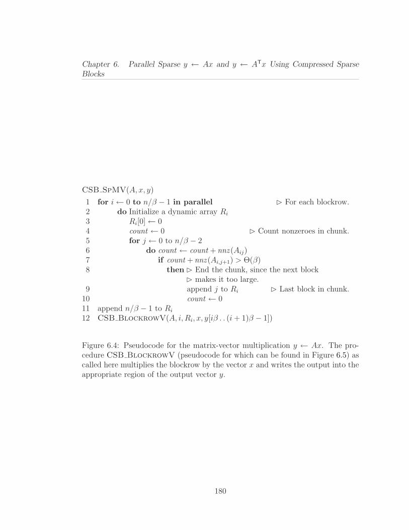
Chapter 6. Parallel Sparse y ← Ax and y ← ATx Using Compressed Sparse
Blocks
CSB SpMV(A, x, y)
1 for i← 0 to n/β − 1 in parallel For each blockrow.2 do Initialize a dynamic array Ri
3 Ri[0]← 04 count ← 0 Count nonzeroes in chunk.5 for j ← 0 to n/β − 26 do count ← count + nnz (Aij)7 if count + nnz (Ai,j+1) > Θ(β)8 then End the chunk, since the next block
makes it too large.9 append j to Ri Last block in chunk.
10 count ← 011 append n/β − 1 to Ri
12 CSB BlockrowV(A, i, Ri, x, y[iβ . . (i + 1)β − 1])
Figure 6.4: Pseudocode for the matrix-vector multiplication y ← Ax. The pro-cedure CSB BlockrowV (pseudocode for which can be found in Figure 6.5) ascalled here multiplies the blockrow by the vector x and writes the output into theappropriate region of the output vector y.
180

Chapter 6. Parallel Sparse y ← Ax and y ← ATx Using Compressed Sparse
Blocks
at index a and ending at index b. The function nnz (Aij) is a shorthand for
A. blk ptr [f(i, j)+1]−A. blk ptr [f(i, j)], which calculates the number of nonzeros
in the block Aij. For conciseness, we have overloaded the Θ(β) notation (in line 7)
to mean “a constant times β”; any constant suffices for the analysis, and we use
the constant 3 in our implementation. The “for . . . in parallel do” construct
means that each iteration of the for loop may be executed in parallel with the
others.
For each loop iteration, we partition the blockrow into chunks in lines 2–11 and
then call the blockrow multiplication in line 12. The array Ri stores the indices
of the last block in each chunk; specifically, the kth chunk, for k > 0, includes
blocks (Ai,Ri[k−1]+1Ai,Ri[k−1]+2 · · ·Ai,Ri[k]). A chunk consists of either a single block
containing Ω(β) nonzeros, or it consists of many blocks containing O(β) nonzeros
in total. To compute chunk boundaries, just iterate over blocks (in lines 5–10)
until enough nonzeros are accrued.
Figure 6.5 gives the parallel algorithm CSB BlockrowV for multiplying
a blockrow by a vector, writing the result into the length-β vector y. The
in parallel do . . .do . . . construct indicates that all of the do code blocks may
execute in parallel. The procedure CSB BlockV (pseudocode for which can be
found in Figure 6.6) calculates the product of the block and the vector in paral-
lel. In lines 12–19 of CSB BlockrowV, the algorithm recursively divides the
181

Chapter 6. Parallel Sparse y ← Ax and y ← ATx Using Compressed Sparse
Blocks
CSB BlockrowV(A, i, R, x, y)
1 if R. length = 2 The subblockrow is a single chunk.2 then ℓ← R[0] + 1 Leftmost block in chunk.3 r ← R[1] Rightmost block in chunk.4 if ℓ = r5 then The chunk is a single (dense) block.6 start ← A. blk ptr [f(i, ℓ)]7 end ← A. blk ptr [f(i, ℓ) + 1]− 18 CSB BlockV(A, start , end , β, x, y)9 else The chunk is sparse.
10 multiply y ← (AiℓAi,ℓ+1 · · ·Air)x serially11 return
Since the block row is “dense,” split it in half.12 mid ← ⌈R. length /2⌉ − 1 Divide chunks in half.
Calculate the dividing point in the input vector x.13 xmid ← β · (R[mid ]−R[0])14 allocate a length-β temporary vector z, initialized to 015 in parallel16 do CSB BlockrowV(A, i, R[0 . .mid ], x[0 . . xmid −1], y)17 do CSB BlockrowV(A, i, R[mid . . R. length −1],
x[xmid . . x. length −1], z)18 for k ← 0 to β − 119 do y[k]← y[k] + z[k]
Figure 6.5: Pseudocode for the subblockrow vector product y ← (AiℓAi,ℓ+1 · · ·Air)x.
182
Chapter 6. Parallel Sparse y ← Ax and y ← ATx Using Compressed Sparse
Blocks
blockrow such that each half receives roughly the same number of chunks. We
find the appropriate middles of the chunk array R and the input vector x in lines
12 and 13, respectively. We then allocate a length-β temporary vector z (line 14)
and perform the recursive multiplications on each subblockrow in parallel (lines
15–17), having one of the recursive multiplications write its output to z. When
these recursive multiplications complete, we merge the outputs into the vector y
(lines 18–19).
The recursion bottoms out when the blockrow consists of a single chunk (lines
2–11). If this chunk contains many blocks, it is guaranteed to contain at most
Θ(β) nonzeros, which is sufficiently sparse to perform the serial multiplication
in line 10. If, on the other hand, the chunk is a single block, it may contain
as many as β2 ≈ n nonzeros. A serial multiplication here, therefore, would be
the bottleneck in the algorithm. Instead, we perform the parallel block-vector
multiplication CSB BlockV in line 8.
If the blockrow recursion reaches a single block, we perform a parallel multi-
plication of the block by the vector. Pseudocode for the subblock-vector prod-
uct y ← Mx, is shown in Figure 6.6, where M is the list of tuples stored
in A. val [start . . end ], A. row ind [start . . end ], and A. col ind [start . . end ] in Z-
morton order. The & operator is a bitwise AND of the two operands. The
block-vector multiplication proceeds by recursively dividing the (sub)block M into
183

Chapter 6. Parallel Sparse y ← Ax and y ← ATx Using Compressed Sparse
Blocks
quadrants M00, M01, M10, and M11, each of which is conveniently stored contigu-
ously in the Z-Morton-ordered val , row ind , and col ind arrays between indices
start and end . We perform binary searches to find the appropriate dividing points
in the array in lines 7–9.
To understand the pseudocode, consider the search for the dividing point s2
between M00M01 and M10M11. For any recursively chosen dim × dim matrix M ,
the column indices and row indices of all elements have the same leading lg β −
lg dim bits. Moreover, for those elements in M00M01, the next bit in the row index
is a 0, whereas for those in elements in M10M11, the next bit in the row index is 1.
The algorithm does a binary search for the point at which this bit flips. The cases
for the dividing point between M00 and M01 or M10 and M11 are similar, except
that we focus on the column index instead of the row index.
After dividing the matrix into quadrants, we execute the matrix products in-
volving matrices M00 and M11 in parallel (lines 10–12), as they do not conflict on
any outputs. After completing these products, we execute the other two matrix
products in parallel (lines 13–15).5 This procedure resembles a standard parallel
divide-and-conquer matrix multiplication, except that our base case of serial mul-
tiplication starts at a matrix containing Θ(dim) nonzeros (lines 2–5). Note that
5The algorithm may instead do M00 and M10 in parallel followed by M01 and M11 in parallelwithout affecting the performance analysis. Presenting the algorithm with two choices may yieldbetter load balance.
184
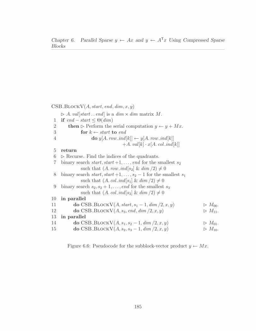
Chapter 6. Parallel Sparse y ← Ax and y ← ATx Using Compressed Sparse
Blocks
CSB BlockV(A, start , end , dim, x, y)
A. val [start . . end ] is a dim × dim matrix M .1 if end − start ≤ Θ(dim)2 then Perform the serial computation y ← y + Mx.3 for k ← start to end4 do y[A. row ind [k]]← y[A. row ind [k]]
+A. val [k] · x[A. col ind [k]]5 return6 Recurse. Find the indices of the quadrants.7 binary search start , start +1, . . . , end for the smallest s2
such that (A. row ind [s2] & dim /2) 6= 08 binary search start , start +1, . . . , s2 − 1 for the smallest s1
such that (A. col ind [s1] & dim /2) 6= 09 binary search s2, s2 + 1, . . . , end for the smallest s3
such that (A. col ind [s3] & dim /2) 6= 010 in parallel11 do CSB BlockV(A, start , s1 − 1, dim /2, x, y) M00.12 do CSB BlockV(A, s3, end , dim /2, x, y) M11.13 in parallel14 do CSB BlockV(A, s1, s2 − 1, dim /2, x, y) M01.15 do CSB BlockV(A, s2, s3 − 1, dim /2, x, y) M10.
Figure 6.6: Pseudocode for the subblock-vector product y ←Mx.
185

Chapter 6. Parallel Sparse y ← Ax and y ← ATx Using Compressed Sparse
Blocks
although we pass the full length-β arrays x and y to each recursive call, the ef-
fective length of each array is halved implicitly by partitioning M into quadrants.
Passing the full arrays is a technical detail required to properly compute array
indices, as the indices A. row ind and A. col ind store offsets within the block.
The CSB SpMV T algorithm is identical to CSB SpMV, except that we
operate over blockcolumns rather than blockrows.
6.5 Analysis
In this section, we prove that for an n×n matrix with nnz nonzeros, CSB SpMV
operates with work Θ(nnz ) and span O(√
n lg n) when β =√
n, yielding a paral-
lelism of Ω(nnz /√
n lg n). We also provide bounds in terms of β and analyze the
space usage.
We begin by analyzing block-vector multiplication.
Lemma 4. On a β × β block containing r nonzeros, CSB BlockV runs with
work Θ(r) and span O(β).
Proof. The span for multiplying a dim × dim matrix can be described by the
recurrence S(dim) = 2S(dim /2) + O(lg dim) = O(dim). The lg dim term repre-
sents a loose upper bound on the cost of the binary searches. In particular, the
186
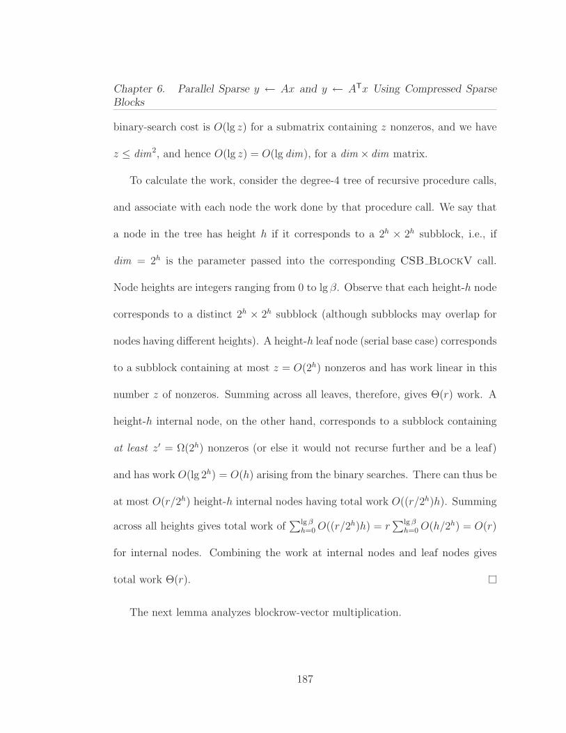
Chapter 6. Parallel Sparse y ← Ax and y ← ATx Using Compressed Sparse
Blocks
binary-search cost is O(lg z) for a submatrix containing z nonzeros, and we have
z ≤ dim2, and hence O(lg z) = O(lg dim), for a dim × dim matrix.
To calculate the work, consider the degree-4 tree of recursive procedure calls,
and associate with each node the work done by that procedure call. We say that
a node in the tree has height h if it corresponds to a 2h × 2h subblock, i.e., if
dim = 2h is the parameter passed into the corresponding CSB BlockV call.
Node heights are integers ranging from 0 to lg β. Observe that each height-h node
corresponds to a distinct 2h × 2h subblock (although subblocks may overlap for
nodes having different heights). A height-h leaf node (serial base case) corresponds
to a subblock containing at most z = O(2h) nonzeros and has work linear in this
number z of nonzeros. Summing across all leaves, therefore, gives Θ(r) work. A
height-h internal node, on the other hand, corresponds to a subblock containing
at least z′ = Ω(2h) nonzeros (or else it would not recurse further and be a leaf)
and has work O(lg 2h) = O(h) arising from the binary searches. There can thus be
at most O(r/2h) height-h internal nodes having total work O((r/2h)h). Summing
across all heights gives total work of∑lg β
h=0 O((r/2h)h) = r∑lg β
h=0 O(h/2h) = O(r)
for internal nodes. Combining the work at internal nodes and leaf nodes gives
total work Θ(r).
The next lemma analyzes blockrow-vector multiplication.
187
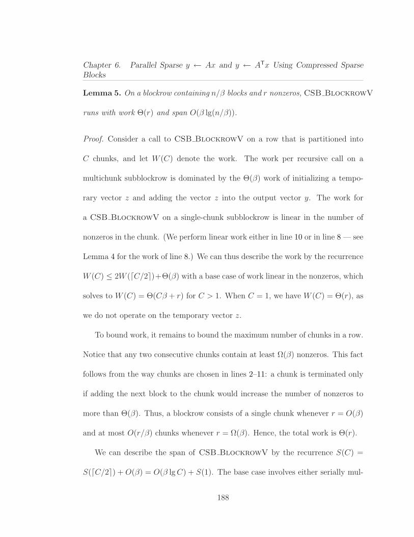
Chapter 6. Parallel Sparse y ← Ax and y ← ATx Using Compressed Sparse
Blocks
Lemma 5. On a blockrow containing n/β blocks and r nonzeros, CSB BlockrowV
runs with work Θ(r) and span O(β lg(n/β)).
Proof. Consider a call to CSB BlockrowV on a row that is partitioned into
C chunks, and let W (C) denote the work. The work per recursive call on a
multichunk subblockrow is dominated by the Θ(β) work of initializing a tempo-
rary vector z and adding the vector z into the output vector y. The work for
a CSB BlockrowV on a single-chunk subblockrow is linear in the number of
nonzeros in the chunk. (We perform linear work either in line 10 or in line 8 — see
Lemma 4 for the work of line 8.) We can thus describe the work by the recurrence
W (C) ≤ 2W (⌈C/2⌉)+Θ(β) with a base case of work linear in the nonzeros, which
solves to W (C) = Θ(Cβ + r) for C > 1. When C = 1, we have W (C) = Θ(r), as
we do not operate on the temporary vector z.
To bound work, it remains to bound the maximum number of chunks in a row.
Notice that any two consecutive chunks contain at least Ω(β) nonzeros. This fact
follows from the way chunks are chosen in lines 2–11: a chunk is terminated only
if adding the next block to the chunk would increase the number of nonzeros to
more than Θ(β). Thus, a blockrow consists of a single chunk whenever r = O(β)
and at most O(r/β) chunks whenever r = Ω(β). Hence, the total work is Θ(r).
We can describe the span of CSB BlockrowV by the recurrence S(C) =
S(⌈C/2⌉) + O(β) = O(β lg C) + S(1). The base case involves either serially mul-
188
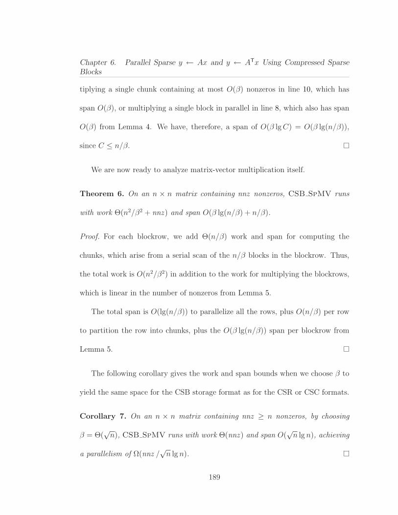
Chapter 6. Parallel Sparse y ← Ax and y ← ATx Using Compressed Sparse
Blocks
tiplying a single chunk containing at most O(β) nonzeros in line 10, which has
span O(β), or multiplying a single block in parallel in line 8, which also has span
O(β) from Lemma 4. We have, therefore, a span of O(β lg C) = O(β lg(n/β)),
since C ≤ n/β.
We are now ready to analyze matrix-vector multiplication itself.
Theorem 6. On an n × n matrix containing nnz nonzeros, CSB SpMV runs
with work Θ(n2/β2 + nnz ) and span O(β lg(n/β) + n/β).
Proof. For each blockrow, we add Θ(n/β) work and span for computing the
chunks, which arise from a serial scan of the n/β blocks in the blockrow. Thus,
the total work is O(n2/β2) in addition to the work for multiplying the blockrows,
which is linear in the number of nonzeros from Lemma 5.
The total span is O(lg(n/β)) to parallelize all the rows, plus O(n/β) per row
to partition the row into chunks, plus the O(β lg(n/β)) span per blockrow from
Lemma 5.
The following corollary gives the work and span bounds when we choose β to
yield the same space for the CSB storage format as for the CSR or CSC formats.
Corollary 7. On an n × n matrix containing nnz ≥ n nonzeros, by choosing
β = Θ(√
n), CSB SpMV runs with work Θ(nnz ) and span O(√
n lg n), achieving
a parallelism of Ω(nnz /√
n lg n).
189
Chapter 6. Parallel Sparse y ← Ax and y ← ATx Using Compressed Sparse
Blocks
Since CSB SpMV T is isomorphic to CSB SpMV, we obtain the following
corollary.
Corollary 8. On an n×n matrix containing nnz ≥ n nonzeros, by choosing β =
Θ(√
n), CSB SpMV T runs with work Θ(nnz ) and span O(√
n lg n), achieving
a parallelism of Ω(nnz /√
n lg n).
The work of our algorithm is dominated by the space of the temporary vec-
tors z, and thus the space usage on an infinite number of processors matches the
work bound. When run on fewer processors however, the space usage reduces dras-
tically. We can analyze the space in terms of the serialization of the program,
which corresponds to the program obtained by removing all parallel keywords.
Lemma 9. On an n × n matrix, by choosing β = Θ(√
n), the serialization of
CSB SpMV requires O(√
n lg n) space (not counting the storage for the matrix
itself).
Proof. The serialization executes one blockrow multiplication at a time. There are
two space overheads. First, we use O(n/β) = O(√
n) space for the chunk array.
Second, we use β space to store the temporary vector z for each outstanding
recursive call to CSB BlockrowV. Since the recursion depth is O(lg n), the
total space becomes O(β lg n) = O(√
n lg n).
190
Chapter 6. Parallel Sparse y ← Ax and y ← ATx Using Compressed Sparse
Blocks
A typical work-stealing scheduler executes the program in a depth-first (serial)
manner on each processor. When a processor completes all its work, it “steals”
work from a different processor, beginning a depth-first execution from some un-
executed parallel branch. Although not all work-stealing schedulers are space
efficient, those maintaining the busy-leaves property [36] (e.g., as used in the
Cilk work-stealing scheduler [35]) are space efficient. The “busy-leaves” prop-
erty roughly says that if a procedure has begun (but not completed) executing,
then there exists a processor currently working on that procedure or one of its
descendants procedures.
Corollary 10. Suppose that a work-stealing scheduler with the busy-leaves prop-
erty schedules an execution of CSB SpMV on an n × n matrix with the choice
β =√
n. Then, the execution requires O(P√
n lg n) space.
Proof. Combine Lemma 9 and Theorem 1 from [35].
The work overhead of our algorithm may be reduced by increasing the con-
stants in the Θ(β) threshold in line 7. Specifically, increasing this threshold by
a constant factor reduces the number of reads and writes to temporaries by the
same constant factor. As these temporaries constitute the majority of the work
overhead of the algorithm, doubling the threshold nearly halves the overhead. In-
191
Chapter 6. Parallel Sparse y ← Ax and y ← ATx Using Compressed Sparse
Blocks
creasing the threshold, however, also increases the span by a constant factor, and
so there is a trade-off.
6.6 Experimental design
This section describes our implementation of the CSB SpMV and CSB SpMV T
algorithms, the benchmark matrices we used to test the algorithms, the machines
on which we ran our tests, and the other codes with which we compared our
algorithms.
Implementation
We parallelized our code using Cilk++ [62], which is a faithful extension of
C++ for multicore and shared-memory parallel programming. Cilk++ is based
on the earlier MIT Cilk system [98], and it employs dynamic load balancing and
provably optimal task scheduling. The CSB code used for the experiments is freely
available for academic use at http://gauss.cs.ucsb.edu/~aydin/software.
html.
The row ind and col ind arrays of CSB, which store the row and column
indices of each nonzero within a block (i.e., the lower-order bits of the row and
column indices within the matrix A), are implemented as a single index array
192
Chapter 6. Parallel Sparse y ← Ax and y ← ATx Using Compressed Sparse
Blocks
by concatenating the two values together. The higher-order bits of row ind and
col ind are stored only implicitly, and are retrieved by referencing the blk ptr
array.
The CSB blocks themselves are stored in row-major order, while the nonzeros
within blocks are in Z-Morton order. The row-major ordering among blocks may
seem to break the overall symmetry of CSB, but in practice it yields efficient han-
dling of block indices for look-up in A. blk ptr by permitting an easily computed
look-up function f(i, j). The row-major ordering also allowed us to count the
nonzeros in a subblockrow more easily when computing y ← Ax. This optimiza-
tion is not symmetric, but interestingly, we achieved similar performance when
computing y ← ATx, where we must still aggregate the nonzeros in each block.
In fact, in almost half the cases, computing ATx was faster than Ax, depending
on the matrix structure.
The Z-Morton ordering on nonzeros in each block is equivalent to first inter-
leaving the bits of row ind and col ind , and then sorting the nonzeros using these
bit-interleaved values as the keys. Thus, it is tempting to store the index array
in a bit-interleaved fashion, thereby simplifying the binary searches in lines 7–9.
Converting to and from bit-interleaved integers, however, is expensive with cur-
rent hardware support,6 which would be necessary for the serial base case in lines
6Recent research [166] addresses these conversions.
193
Chapter 6. Parallel Sparse y ← Ax and y ← ATx Using Compressed Sparse
Blocks
2–5. Instead, the kth element of the index array is the concatenation of row ind [k]
and col ind [k], as indicated earlier. This design choice of storing concatenated,
instead of bit-interleaved, indices requires either some care when performing the
binary search (as presented in Figure 6.6) or implicitly converting from the con-
catenated to interleaved format when making a binary-search comparison. Our
preliminary implementation does the latter, using a C++ function object for com-
parisons [188]. In practice, the overhead of performing these conversions is small,
since the number of binary-search steps is small.
Performing the actual address calculation and determining the pointers to x
and y vectors are done by masking and bit-shifting. The bitmasks are deter-
mined dynamically by the CSB constructor depending on the input matrix and
the data type used for storing matrix indices. Our library allows any data type
to be used for matrix indices and handles any type of matrix dynamically. For
the results presented in Section 6.7, nonzero values are represented as double-
precision floating-point numbers, and indices are represented as 32-bit unsigned
integers. Finally, as our library aims to be general instead of matrix specific, we
did not employ speculative low-level optimizations such as software prefetching,
pipelining, or matrix-specific optimizations such as index and/or value compres-
sion [131, 207], but we believe that CSB and our algorithms should not adversely
affect incorporation of these approaches.
194
Chapter 6. Parallel Sparse y ← Ax and y ← ATx Using Compressed Sparse
Blocks
Choosing the block size β
We investigated different strategies to choose the block size that achieves the
best performance. For the types of loads we ran, we found that a block size
slightly larger than√
n delivers reasonable performance. Figure 6.7 shows the
effect of different blocksizes on the performance of the y ← Ax operation with
the representative matrix Kkt power. The closest exact power of 2 to√
n is
1024, which turns out to be slightly suboptimal. In our experiments, the overall
best performance was achieved when β satisfies the equation ⌈lg√n⌉ ≤ lg β ≤
3 + ⌈lg√n⌉.
Merely setting β to a hard-coded value, however, is not robust for various
reasons. First, the elements stored in the index array should use the same data
type as that used for matrix indices. Specifically, the integer β − 1 should fit in
2 bytes so that a concatenated row ind and col ind fit into 4 bytes. Second, the
length-β regions of the input vector x and output vector y (which are accessed
when multiplying a single block) should comfortably fit into L2 cache. Finally,
to ensure speedup on matrices with evenly distributed nonzeros, there should be
enough parallel slackness for the parallelization across blockrows (i.e., the highest
level parallelism). Specifically, when β grows large, the parallelism is roughly
bounded by O(nnz /(β lg(n/β))) (by dividing the work and span from Theorem 6).
195

Chapter 6. Parallel Sparse y ← Ax and y ← ATx Using Compressed Sparse
Blocks
0
100
200
300
400
500
32 64
128 256
512 1024
2048 4096
8192 16384
32768
MF
lops
/sec
Block size
p=8p=4p=2
Figure 6.7: The effect of block size parameter β on SpMV performance using the
Kkt power matrix. For values β > 32768 and β < 32, the experiment failed to
finish due to memory limitations. The experiment was conducted on the AMD
Opteron.
Thus, we want nnz /(β lg(n/β)) to be “large enough,” which means limiting the
maximum magnitude of β.
We adjusted our CSB constructor, therefore, to automatically select a reason-
able block-size parameter β. It starts with β = 3 + ⌈lg√n⌉ and keeps decreasing
it until the aforementioned constraints are satisfied. Although a research opportu-
nity may exist to autotune the optimal block size with respect to a specific matrix
and architecture, in most test matrices, choosing β =√
n degraded performance
by at most 10%–15%. The optimal β value barely shifts along the x-axis when
running on different numbers of processors and is quite stable overall.
196

Chapter 6. Parallel Sparse y ← Ax and y ← ATx Using Compressed Sparse
Blocks
An optimization heuristic for structured matrices
Even though CSB SpMV and CSB SpMV T are robust and exhibit plenty
of parallelism on most matrices, their practical performance can be improved on
some sparse matrices having regular structure. In particular, a block diagonal
matrix with equally sized blocks has nonzeros that are evenly distributed across
blockrows. In this case, a simple algorithm based on blockrow parallelism would
suffice in place of the more complicated recursive method from CSB BlockV.
This divide-and-conquer within blockrows incurs overhead that might unnecessar-
ily degrade performance. Thus, when the nonzeros are evenly distributed across
the blockrows, our implementation of the top-level algorithm (given in Figure 6.4)
calls the serial multiplication in line 12 instead of the CSB BlockrowV proce-
dure.
To see whether a given matrix is amenable to the optimization, we apply the
following “balance” heuristic. We calculate the imbalance among blockrows (or
blockcolumns in the case of y ← ATx) and apply the optimization only when no
blocks have more than twice the average number of nonzeros per blockrow. In
other words, if max(nnz (Ai)) < 2 · mean(nnz (Ai)), then the matrix is consid-
ered to have balanced blockrows and the optimization is applied. Of course, this
optimization is not the only way to achieve a performance boost on structured
matrices.
197
Chapter 6. Parallel Sparse y ← Ax and y ← ATx Using Compressed Sparse
Blocks
Optimization of temporary vectors
One of the most significant overheads of our algorithm is the use of temporary
vectors to store intermediate results when parallelizing a blockrow multiplication
in CSB BlockRowV. The “balance” heuristic above is one way of reducing this
overhead when the nonzeros in the matrix are evenly distributed. For arbitrary
matrices, however, we can still reduce the overhead in practice. In particular, we
only need to allocate the temporary vector z (in line 14) if both of the subsequent
multiplications (lines 15–17) are scheduled in parallel. If the first recursive call
completes before the second recursive call begins, then we instead write directly
into the output vector for both recursive calls. In other words, when a blockrow
multiplication is scheduled serially, the multiplication procedure detects this fact
and mimics a normal serial execution, without the use of temporary vectors. Our
implementation exploits an undocumented feature of Cilk++ to test whether the
first call has completed before making the second recursive call, and we allocate
the temporary as appropriate. This test may also be implemented using Cilk++
reducers [97].
Sparse-matrix test suite
We conducted experiments on a diverse set of sparse matrices from real appli-
cations including circuit simulation, finite-element computations, linear program-
198
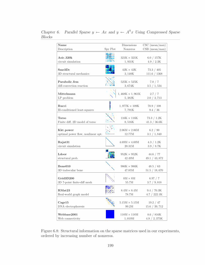
Chapter 6. Parallel Sparse y ← Ax and y ← ATx Using Compressed Sparse
Blocks
Name
Spy Plot
Dimensions CSC (mean/max)
Description Nonzeros CSB (mean/max)
Asic 320k 321K× 321K 6.0 / 157K
circuit simulation 1, 931K 4.9 / 2.3K
Sme3Dc 42K× 42K 73.3 / 405
3D structural mechanics 3, 148K 111.6 / 1368
Parabolic fem 525K× 525K 7.0 / 7
diff-convection reaction 3, 674K 3.5 / 1, 534
Mittelmann 1, 468K× 1, 961K 2.7 / 7
LP problem 5, 382K 2.0 / 3, 713
Rucci 1, 977K× 109K 70.9 / 108
Ill-conditioned least-squares 7, 791K 9.4 / 36
Torso 116K× 116K 73.3 / 1.2K
Finite diff, 2D model of torso 8, 516K 41.3 / 36.6K
Kkt power 2.06M× 2.06M 6.2 / 90
optimal power flow, nonlinear opt. 12.77M 3.1 / 1, 840
Rajat31 4.69M× 4.69M 4.3 / 1.2K
circuit simulation 20.31M 3.9 / 8.7K
Ldoor 952K× 952K 44.6 / 77
structural prob. 42.49M 49.1 / 43, 872
Bone010 986K× 986K 48.5 / 63
3D trabecular bone 47.85M 51.5 / 18, 670
Grid3D200 8M× 8M 6.97 / 7
3D 7-point finite-diff mesh 55.7M 3.7 / 9, 818
RMat23 8.4M× 8.4M 9.4 / 70.3K
Real-world graph model 78.7M 4.7 / 222.1K
Cage15 5.15M× 5.15M 19.2 / 47
DNA electrophoresis 99.2M 15.6 / 39, 712
Webbase2001 118M× 118M 8.6 / 816K
Web connectivity 1, 019M 4.9 / 2, 375K
Figure 6.8: Structural information on the sparse matrices used in our experiments,ordered by increasing number of nonzeros.
199
Chapter 6. Parallel Sparse y ← Ax and y ← ATx Using Compressed Sparse
Blocks
ming, and web-connectivity analysis. These matrices not only cover a wide range
of applications, but they also greatly vary in size, density, and structure. The test
suite contains both rectangular and square matrices. Almost half of the square
matrices are asymmetric. Figure 6.8 summarizes the 14 test matrices. The first
ten matrices and Cage15 are from the University of Florida sparse matrix collec-
tion [73]. Grid3D200 is a 7-point finite difference mesh generated using the Matlab
Mesh Partitioning and Graph Separator Toolbox [103]. The RMat23 matrix [140],
which models scale-free graphs, is generated by using repeated Kronecker prod-
ucts [16]. We chose parameters A = 0.7, B = C = D = 0.1 for RMat23 in order
to generate skewed matrices. Webbase2001 is a crawl of the World Wide Web
from the year 2001 [59].
Included in Figure 6.8 is the load imbalance that is likely to occur for an
SpMV algorithm parallelized with respect to columns (CSC) and blocks (CSB).
In the last column, the average (mean) and the maximum number of nonzeros
among columns (first line) and blocks (second line) are shown for each matrix.
The sparsity of matrices can be quantified by the average number of nonzeros per
column, which is equivalent to the mean of CSC. The sparsest matrix (Rajat31)
has 4.3 nonzeros per column on the average while the densest matrix has about
73 nonzeros per column (Sme3Dc and Torso). For CSB, the reported mean/max
200
Chapter 6. Parallel Sparse y ← Ax and y ← ATx Using Compressed Sparse
Blocks
values are obtained by setting the block dimension β to be approximately√
n, so
that they are comparable with statistics from CSC.
Architectures and comparisons
We ran our experiments on three multicore superscalar architectures. Opteron
is a ccNUMA architecture powered by AMD Opteron 8214 (Santa Rosa) processors
clocked at 2.2 GHz. Each core of Opteron has a private 1 MB L2 cache, and each
socket has its own integrated memory controller. Although it is an 8-socket dual-
core system, we only experimented with up to 8 processors. Harpertown is a
dual-socket quad-core system running two Intel Xeon X5460’s, each clocked at
3.16 GHz. Each socket has 12 MB of L2 cache, shared among four cores, and a
front-side bus (FSB) running at 1333 MHz. Nehalem is a single-socket quad-core
Intel Core i7 920 processor. Like Opteron, Nehalem has an integrated memory
controller. Each core is clocked at 2.66 GHz and has a private 256 KB L2 cache.
The four cores share an 8 MB L3 cache.
While Opteron has 64 GB of RAM, Harpertown and Nehalem have only 8GB
and 6 GB, respectively, which forced us to exclude our biggest test matrix (Web-
base2001) from our runs on Intel architectures. We compiled our code using gcc
4.1 on Opteron and Harpertown and with gcc 4.3 on Nehalem, all with opti-
mization flags -O2 -fno-rtti -fno-exceptions.
201
Chapter 6. Parallel Sparse y ← Ax and y ← ATx Using Compressed Sparse
Blocks
To evaluate our code on a single core, we compared its performance with “pure”
OSKI matrix-vector multiplication [205] running on one processor of Opteron.
We did not enable OSKI’s preprocessing step, which chooses blockings for cache
and register usage that are tuned to a specific matrix. We conjecture that such
matrix-specific tuning techniques can be combined advantageously with our CSB
data structure and parallel algorithms.
To compare with a parallel code, we used the matrix-vector multiplication of
Star-P [179] running on Opteron. Star-P is a distributed-memory code that uses
CSR to represent sparse matrices and distributes matrices to processor memories
by equal-sized blocks of rows.
6.7 Experimental results
Figures 6.9 and 6.10 show how CSB SpMV and CSB SpMV T, respectively,
scale for the seven smaller matrices on Opteron, and Figures 6.11 and 6.12 show
similar results for the seven larger matrices. In most cases, the two codes show
virtually identical performance, confirming that the CSB data structure and algo-
rithms are equally suitable for both operations. In all the parallel scaling graphs,
only the values p = 1, 2, 4, 8 are reported. They should be interpreted as perfor-
202
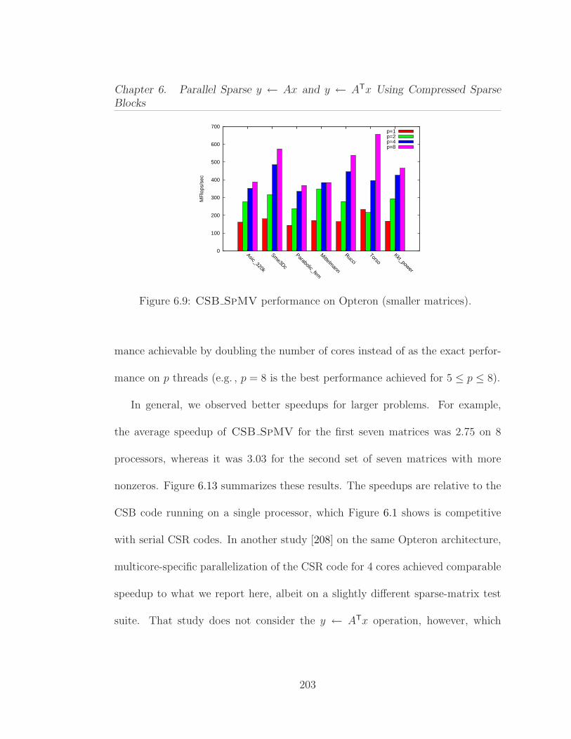
Chapter 6. Parallel Sparse y ← Ax and y ← ATx Using Compressed Sparse
Blocks
0
100
200
300
400
500
600
700
Asic_320k
Sme3Dc
Parabolic_fem
Mittelm
ann
Rucci
TorsoKkt_power
MF
lops
/sec
p=1p=2p=4p=8
Figure 6.9: CSB SpMV performance on Opteron (smaller matrices).
mance achievable by doubling the number of cores instead of as the exact perfor-
mance on p threads (e.g. , p = 8 is the best performance achieved for 5 ≤ p ≤ 8).
In general, we observed better speedups for larger problems. For example,
the average speedup of CSB SpMV for the first seven matrices was 2.75 on 8
processors, whereas it was 3.03 for the second set of seven matrices with more
nonzeros. Figure 6.13 summarizes these results. The speedups are relative to the
CSB code running on a single processor, which Figure 6.1 shows is competitive
with serial CSR codes. In another study [208] on the same Opteron architecture,
multicore-specific parallelization of the CSR code for 4 cores achieved comparable
speedup to what we report here, albeit on a slightly different sparse-matrix test
suite. That study does not consider the y ← ATx operation, however, which
203
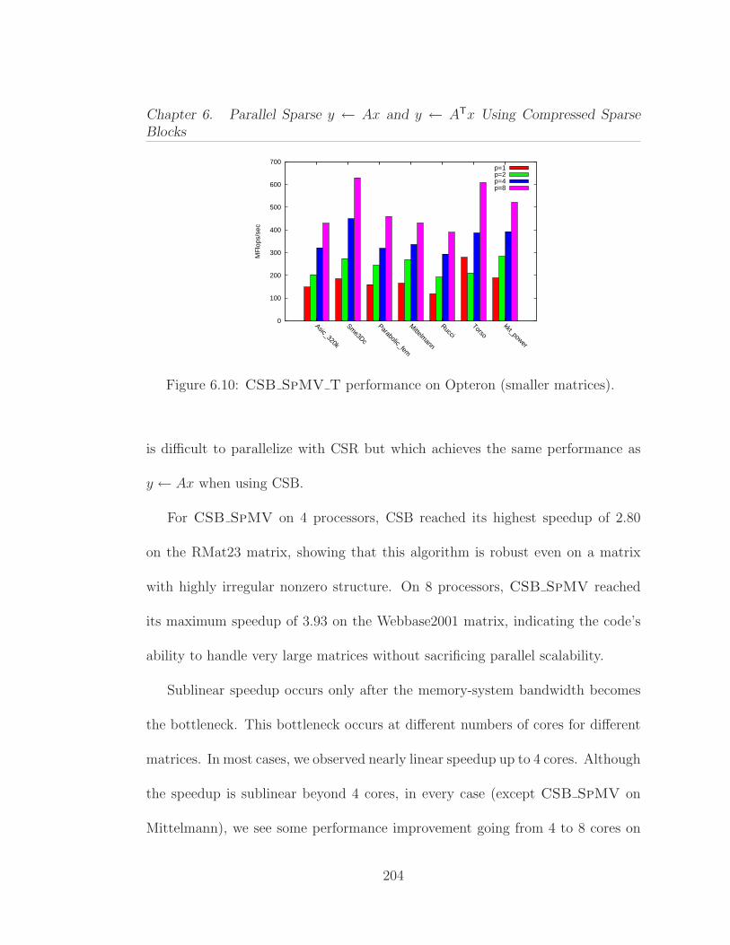
Chapter 6. Parallel Sparse y ← Ax and y ← ATx Using Compressed Sparse
Blocks
0
100
200
300
400
500
600
700
Asic_320k
Sme3Dc
Parabolic_fem
Mittelm
ann
Rucci
Torsokkt_power
MF
lops
/sec
p=1p=2p=4p=8
Figure 6.10: CSB SpMV T performance on Opteron (smaller matrices).
is difficult to parallelize with CSR but which achieves the same performance as
y ← Ax when using CSB.
For CSB SpMV on 4 processors, CSB reached its highest speedup of 2.80
on the RMat23 matrix, showing that this algorithm is robust even on a matrix
with highly irregular nonzero structure. On 8 processors, CSB SpMV reached
its maximum speedup of 3.93 on the Webbase2001 matrix, indicating the code’s
ability to handle very large matrices without sacrificing parallel scalability.
Sublinear speedup occurs only after the memory-system bandwidth becomes
the bottleneck. This bottleneck occurs at different numbers of cores for different
matrices. In most cases, we observed nearly linear speedup up to 4 cores. Although
the speedup is sublinear beyond 4 cores, in every case (except CSB SpMV on
Mittelmann), we see some performance improvement going from 4 to 8 cores on
204
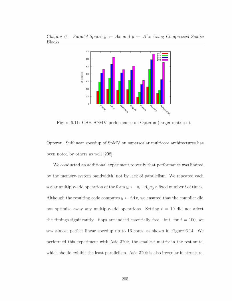
Chapter 6. Parallel Sparse y ← Ax and y ← ATx Using Compressed Sparse
Blocks
0
100
200
300
400
500
600
700
Rajat31
Ldoor
Grid3D200
Cage15
RMat23
Bone010
Webbase2001
MF
lops
/sec
p=1p=2p=4p=8
Figure 6.11: CSB SpMV performance on Opteron (larger matrices).
Opteron. Sublinear speedup of SpMV on superscalar multicore architectures has
been noted by others as well [208].
We conducted an additional experiment to verify that performance was limited
by the memory-system bandwidth, not by lack of parallelism. We repeated each
scalar multiply-add operation of the form yi ← yi+Aijxj a fixed number t of times.
Although the resulting code computes y ← tAx, we ensured that the compiler did
not optimize away any multiply-add operations. Setting t = 10 did not affect
the timings significantly—flops are indeed essentially free—but, for t = 100, we
saw almost perfect linear speedup up to 16 cores, as shown in Figure 6.14. We
performed this experiment with Asic 320k, the smallest matrix in the test suite,
which should exhibit the least parallelism. Asic 320k is also irregular in structure,
205

Chapter 6. Parallel Sparse y ← Ax and y ← ATx Using Compressed Sparse
Blocks
0
100
200
300
400
500
600
700
800
Rajat31
Ldoor
Grid3D200
Cage15
RMat23
Bone010
Webbase2001
MF
lops
/sec
p=1p=2p=4p=8
Figure 6.12: CSB SpMV T performance on Opteron (larger matrices).
ProcessorsCSB SpMV CSB SpMV T
1–7 8–14 1–7 8–14
P = 2 1.65 1.70 1.44 1.49
P = 4 2.34 2.49 2.07 2.30
P = 8 2.75 3.03 2.81 3.16
Figure 6.13: Average speedup results for relatively smaller (1–7) and larger (8–14)matrices. These experiments were conducted on Opteron.
which means that our balance heuristic does not apply. Nevertheless, CSB SpMV
scaled almost perfectly given enough flops per byte.
The parallel performance of CSB SpMV and CSB SpMV T is generally not
affected by highly uneven row and column nonzero counts. The highly skewed
matrices RMat23 and Webbase2001 achieved speedups as good as for matrices
with flat row and column counts. An unusual case is the Torso matrix, where
both CSB SpMV and CSB SpMV T were actually slower on 2 processors than
206
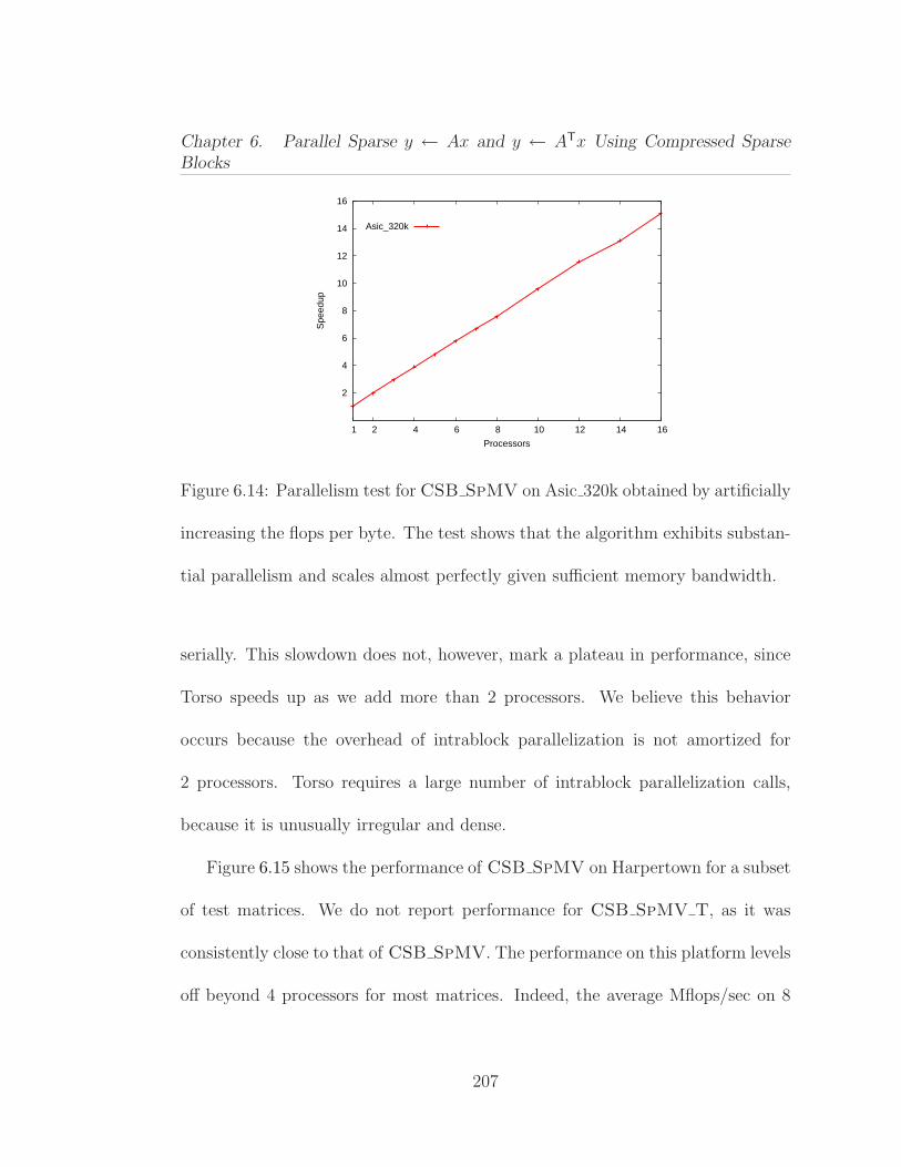
Chapter 6. Parallel Sparse y ← Ax and y ← ATx Using Compressed Sparse
Blocks
2
4
6
8
10
12
14
16
1 2 4 6 8 10 12 14 16
Spe
edup
Processors
Asic_320k
Figure 6.14: Parallelism test for CSB SpMV on Asic 320k obtained by artificially
increasing the flops per byte. The test shows that the algorithm exhibits substan-
tial parallelism and scales almost perfectly given sufficient memory bandwidth.
serially. This slowdown does not, however, mark a plateau in performance, since
Torso speeds up as we add more than 2 processors. We believe this behavior
occurs because the overhead of intrablock parallelization is not amortized for
2 processors. Torso requires a large number of intrablock parallelization calls,
because it is unusually irregular and dense.
Figure 6.15 shows the performance of CSB SpMV on Harpertown for a subset
of test matrices. We do not report performance for CSB SpMV T, as it was
consistently close to that of CSB SpMV. The performance on this platform levels
off beyond 4 processors for most matrices. Indeed, the average Mflops/sec on 8
207
Chapter 6. Parallel Sparse y ← Ax and y ← ATx Using Compressed Sparse
Blocks
processors is only 3.5% higher than on 4 processors. We believe this plateau results
from insufficient memory bandwidth. The continued speedup on Opteron is due
to its higher ratio of memory bandwidth (bytes) to peak performance (flops) per
second.
Figure 6.16 summarizes the performance results of CSB SpMV for the same
subset of test matrices on Nehalem. Despite having only 4 physical cores, for most
matrices, Nehalem achieved scaling up to 8 threads thanks to hyperthreading.
Running 8 threads was necessary to utilize the processor fully, because hyper-
threading fills the pipeline more effectively. We observed that the improvement
from oversubscribing is not monotonic, however, because running more threads
reduces the effective cache size available to each thread. Nehalem’s point-to-point
interconnect is faster than Opteron’s (a generation old Hypertransport 1.0), which
explains its better speedup values when comparing the 4-core performance of both
architectures. Its raw performance is also impressive, beating both Opteron and
Harpertown by large margins.
To determine CSB’s competitiveness with a conventional CSR code, we com-
pared the performance of the CSB serial code with plain OSKI using no matrix-
specific optimizations such as register or cache blocking. Figures 6.17 and 6.18
present the results of the comparison. As can be seen from the figures, CSB
achieves similar serial performance to CSR.
208
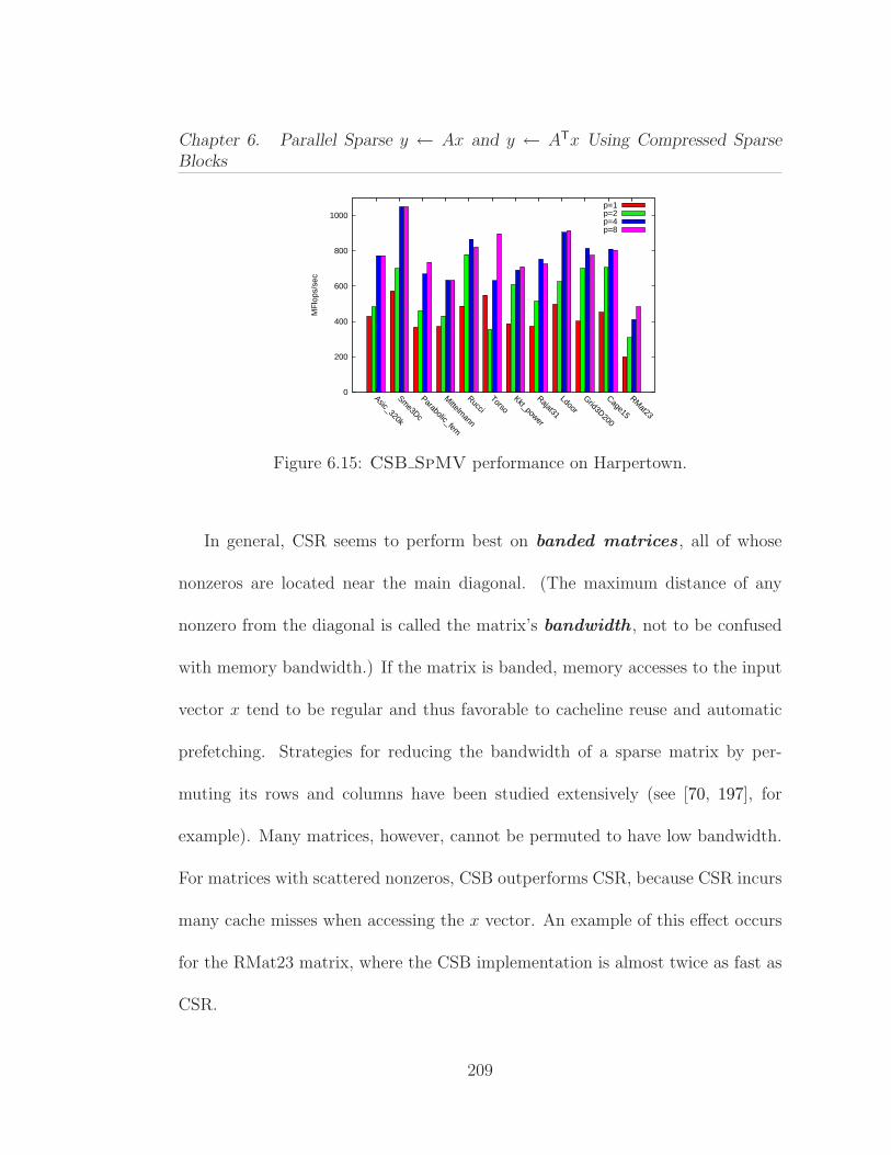
Chapter 6. Parallel Sparse y ← Ax and y ← ATx Using Compressed Sparse
Blocks
0
200
400
600
800
1000
Asic_320k
Sme3Dc
Parabolic_fem
Mittelm
ann
Rucci
TorsoKkt_power
Rajat31
Ldoor
Grid3D200
Cage15
RMat23
MF
lops
/sec
p=1p=2p=4p=8
Figure 6.15: CSB SpMV performance on Harpertown.
In general, CSR seems to perform best on banded matrices , all of whose
nonzeros are located near the main diagonal. (The maximum distance of any
nonzero from the diagonal is called the matrix’s bandwidth , not to be confused
with memory bandwidth.) If the matrix is banded, memory accesses to the input
vector x tend to be regular and thus favorable to cacheline reuse and automatic
prefetching. Strategies for reducing the bandwidth of a sparse matrix by per-
muting its rows and columns have been studied extensively (see [70, 197], for
example). Many matrices, however, cannot be permuted to have low bandwidth.
For matrices with scattered nonzeros, CSB outperforms CSR, because CSR incurs
many cache misses when accessing the x vector. An example of this effect occurs
for the RMat23 matrix, where the CSB implementation is almost twice as fast as
CSR.
209

Chapter 6. Parallel Sparse y ← Ax and y ← ATx Using Compressed Sparse
Blocks
0
500
1000
1500
2000
Asic_320k
Sme3Dc
Parabolic_fem
Mittelm
ann
Rucci
TorsoKkt_power
Rajat31
Ldoor
Grid3D200
Cage15
RMat23
MF
lops
/sec
p=1p=2p=4p=8
Figure 6.16: CSB SpMV performance on Nehalem.
Figure 6.19 compares the parallel performance of the CSB algorithms with
Star-P. Star-P’s blockrow data distribution does not afford any flexibility for load-
balancing across processors. Load balance is not an issue for matrices with nearly
flat row counts, including finite-element and finite-difference matrices, such as
Grid3D200. Load balance does become an issue for skewed matrices such as
RMat23, however. Our performance results confirm this effect. CSB SpMV is
about 500% faster than Star-P’s SpMV routine for RMat23 on 8 cores. Moreover,
for any number of processors, CSB SpMV runs faster for all the matrices we
tested, including the structured ones.
210
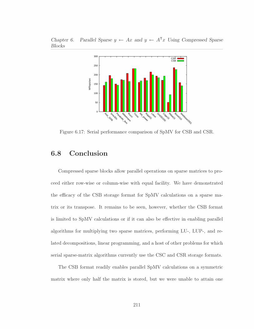
Chapter 6. Parallel Sparse y ← Ax and y ← ATx Using Compressed Sparse
Blocks
0
50
100
150
200
250
300
Asic_320k
Sme3Dc
Parabolic_fem
Mittelm
ann
Rucci
TorsoKkt_power
Rajat31
Ldoor
Grid3D200
Cage15
RMat23
Bone010
Webbase2001
MF
lops
/sec
CSRCSB
Figure 6.17: Serial performance comparison of SpMV for CSB and CSR.
6.8 Conclusion
Compressed sparse blocks allow parallel operations on sparse matrices to pro-
ceed either row-wise or column-wise with equal facility. We have demonstrated
the efficacy of the CSB storage format for SpMV calculations on a sparse ma-
trix or its transpose. It remains to be seen, however, whether the CSB format
is limited to SpMV calculations or if it can also be effective in enabling parallel
algorithms for multiplying two sparse matrices, performing LU-, LUP-, and re-
lated decompositions, linear programming, and a host of other problems for which
serial sparse-matrix algorithms currently use the CSC and CSR storage formats.
The CSB format readily enables parallel SpMV calculations on a symmetric
matrix where only half the matrix is stored, but we were unable to attain one
211
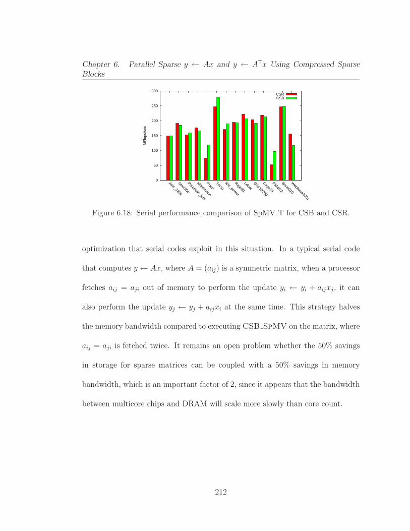
Chapter 6. Parallel Sparse y ← Ax and y ← ATx Using Compressed Sparse
Blocks
0
50
100
150
200
250
300
Asic_320k
Sme3Dc
Parabolic_fem
Mittelm
ann
Rucci
TorsoKkt_power
Rajat31
Ldoor
Grid3D200
Cage15
RMat23
Bone010
Webbase2001
MF
lops
/sec
CSRCSB
Figure 6.18: Serial performance comparison of SpMV T for CSB and CSR.
optimization that serial codes exploit in this situation. In a typical serial code
that computes y ← Ax, where A = (aij) is a symmetric matrix, when a processor
fetches aij = aji out of memory to perform the update yi ← yi + aijxj, it can
also perform the update yj ← yj + aijxi at the same time. This strategy halves
the memory bandwidth compared to executing CSB SpMV on the matrix, where
aij = aji is fetched twice. It remains an open problem whether the 50% savings
in storage for sparse matrices can be coupled with a 50% savings in memory
bandwidth, which is an important factor of 2, since it appears that the bandwidth
between multicore chips and DRAM will scale more slowly than core count.
212
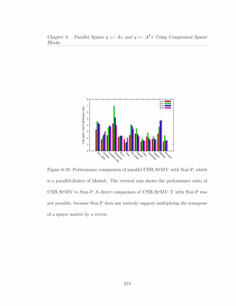
Chapter 6. Parallel Sparse y ← Ax and y ← ATx Using Compressed Sparse
Blocks
0
1
2
3
4
5
6
7
8
Asic_320k
Sme3Dc
Parabolic_fem
Mittelm
ann
Rucci
TorsoKkt_power
Rajat31
Ldoor
Grid3D200
Cage15
RMat23
Bone010
CS
B_S
pMV
/ S
tar-
P (
MF
lops
/sec
rat
io)
p=1p=2p=4p=8
Figure 6.19: Performance comparison of parallel CSB SpMV with Star-P, which
is a parallel-dialect of Matlab. The vertical axis shows the performance ratio of
CSB SpMV to Star-P. A direct comparison of CSB SpMV T with Star-P was
not possible, because Star-P does not natively support multiplying the transpose
of a sparse matrix by a vector.
213
Chapter 7
Solving Path Problems on theGPU
Abstract
We consider the computation of shortest paths on Graphic ProcessingUnits (GPUs). The blocked recursive elimination strategy we use is ap-plicable to a class of algorithms (such as all-pairs shortest-paths, tran-sitive closure, and LU decomposition without pivoting) having similardata access patterns. Using the all-pairs shortest-paths problem as anexample, we uncover potential gains over this class of algorithms. Theimpressive computational power and memory bandwidth of the GPUmake it an attractive platform to run such computationally intensivealgorithms. Although improvements over CPU implementations havepreviously been achieved for those algorithms in terms of raw speed,the utilization of the underlying computational resources was quitelow. We implemented a recursively partitioned all-pairs shortest-pathsalgorithm that harnesses the power of GPUs better than existing im-plementations. The alternate schedule of path computations allowedus to cast almost all operations into matrix-matrix multiplications on asemiring. Since matrix-matrix multiplication is highly optimized andhas a high ratio of computation to communication, our implemen-tation does not suffer from the premature saturation of bandwidthresources as iterative algorithms do. By increasing temporal locality,our implementation runs more than two orders of magnitude faster onan NVIDIA 8800 GPU than on an Opteron. Our work provides evi-dence that programmers should rethink algorithms instead of directlyporting them to GPU.
214
Chapter 7. Solving Path Problems on the GPU
This chapter is based on a paper [50] by Buluc et al. from Parallel Computing.
7.1 Introduction
The massively parallel nature of GPUs makes them capable of yielding the-
oretically much higher GFlops rates than current state-of-the-art CPUs. GPU
performance also grows much faster than CPU performance due to specialized
explicit parallelism. The amount of computational power to be harvested has also
attracted the high-performance computing (HPC) community, and we have seen
many scientific applications successfully implemented with significant performance
gains on the GPU [37, 178].
Implementing HPC applications to run on a GPU requires significant exper-
tise, even with the recently introduced C-like APIs such as Nvidia’s Cuda plat-
form [141]. The key to performance is to hide the data access latency by having
many threads on the fly. The performance is usually fragile and requires careful
craftmanship from the programmer’s side. It is up to the programmer to make
sure that the registers and other levels of cache are neither underutilized nor over-
pressured. Several papers are devoted to the issue of achieving the right balance
to get optimal performance on GPUs [170, 204], relying on novel programming
techniques that are not necessarily intuitive to the existing HPC programmer.
215
Chapter 7. Solving Path Problems on the GPU
An important class of algorithms with triple nested loops, which will be sub-
sequently mentioned as Gaussian Elimination (GE) based algorithms, have very
similar data access patterns. Examples include LU decomposition without pivot-
ing, Cholesky factorization, all-pairs shortest paths (APSP), and transitive clo-
sure. The similarity among those problems has led researchers to approach them
in a unified manner. For example, the Gaussian Elimination Paradigm of Chowd-
hury and Ramachandran provides a cache-oblivious framework for these prob-
lems [60]. In this paper, we specifically focus on the APSP problem because it
usually operates on single precision floating point data, making it suitable to cur-
rent generation GPUs. On the contrary, factorizations such as LU and Cholesky
require double precision arithmetic that was not available on the GPUs until very
recently (with AMD FireStream 9170 and Nvidia GeForce GTX 280). Even now,
the double precision performance is 4-8 times slower than single precision, and
the limited global memory of current generation GPUs discourage the use of dou-
ble precision floating point numbers. Furthermore, numerical LU decomposition
without pivoting is unstable [106] at best (it may not even exist), and pivoting
strategies on the GPU are beyond the scope of this paper. Volkov and Demmel
did an excellent job of implementing LU, QR, and Cholesky factorizations on the
GPU, albeit in single precision [204]. It is worth noting that even though our
implementation computes only the distance version of the APSP problem, it is
216
Chapter 7. Solving Path Problems on the GPU
possible to obtain the actual minimal paths, at the cost of doubling the memory
requirements, by keeping a predecessor matrix.
Our two main contributions in this paper are:
1. Recursive partitioning is used as a tool to express a different schedule of
path computations that allows extensive use of highly optimized matrix-
matrix operations. Specifically, we use matrix multiplication on semirings
as a building block for GE based algorithms. By doing so, we increase data
locality, which is even more important for high performance computing on
the GPU than on the CPU
2. As a proof of concept, we provide an efficient implementation of the APSP
algorithm on the GPU that is up to 480x faster than our reference CPU
implementation, and up to 75x faster than an existing GPU implementation
on a similar architecture.
Locality of reference has always been an issue in algorithm design, and it will
be even more important with GPUs. This is because stream processors, such as
GPUs, achieve efficiency through locality [72]. Our work highlights the importance
of recursion as a technique for automatically creating locality of reference.
As minor contributions, we give an alternate (arguably simpler) proof of cor-
rectness based on path expressions for the recursively partitioned APSP algorithm.
217

Chapter 7. Solving Path Problems on the GPU
On the GPU, we compare iterative, and recursive versions of the same algorithm
and provide insights into their performance difference through micro benchmarks.
Therefore, we provide evidence that Level 3 BLAS [80] routines on semirings can
be used to speed up certain graph algorithms. Finally, we compare different CPUs
and GPUs on their power efficiency in solving this problem.
The remainder of this paper is organized as follows. Section 7.2 describes
the algorithms based on block-recursive elimination, starting from the well-known
Gaussian Elimination procedure and using it as an analogy to explain block-
recursive elimination on other algebraic structures. Most specifically, it shows
how block-recursive elimination can be used to solve the all-pairs shortest-paths
problem. Section 7.3 is devoted to GPU programming on the Cuda platform,
showing difficulties and important points to achieve high performance on GPUs.
Section 7.4 describes our implementation and evaluation strategies, and reports
on the results of our experiments. Section 7.5 offers some concluding remarks.
7.2 Algorithms Based on Block-Recursive Elim-
ination
Gaussian elimination is used to solve a system of linear equations Ax = b,
where A is an n × n matrix of coefficients, x is a vector of unknowns, and b
218

Chapter 7. Solving Path Problems on the GPU
is a vector of constants. Recursive blocked LU factorization is an efficient way
of performing Gaussian elimination on architectures with deep memory hierar-
chies [87, 198]. This is mostly due to its extensive use of matrix-matrix operations
(Level 3 BLAS [80]) that are optimized for the underlying architecture. Let A
and its factors L and U be partitioned as
A =
A11 A12
A21 A22
=
L11
L21 L22
·
U11 U12
U22
(7.1)
Then, the block-recursive LU decomposition without pivoting can be written
as
L11, U11 ←LU(A11)
U12 ←L11\A12 (7.2)
L21 ←A21/U11
L22, U22 ←LU(A22 − L21U12).
In this pseudocode, LU is the recursive call to the function itself, \ and / denote
triangular solve operations with multiple right hand sides (matrix division on the
left and on the right, in Matlab notation).
LU factorization operates on the field of real numbers, but the same algo-
rithm can be used to solve a number of graph problems, albeit using a different
219

Chapter 7. Solving Path Problems on the GPU
algebra. Specifically, closed semirings provide a general algebraic structure that
can be used to solve a number of path problems on graphs [7, 192]. A semiring
has all the properties of a ring, except that there might be elements without an
additive inverse. One practical implication is that fast matrix multiplication al-
gorithms that use additive inverses, such as the Strassen algorithm [187] and the
Coppersmith-Winograd algorithm [67], do not apply to matrices over semirings.
A closed semiring is formally denoted by (S,⊕,⊗, 0, 1), where ⊕ and ⊗ are
binary operations defined on the set S with identity elements 0 and 1 respec-
tively. Fletcher [93] gives a complete definition of a closed semiring. Two im-
portant semirings used in this work are the Boolean semiring, formally defined as
(0, 1,∨,∧, 0, 1) and the tropical semiring, formally defined as (R+, min, +,∞, 0).
A closed semiring is said to be idempotent if a⊕a = a for all a ∈ S. Although idem-
potence of the semiring is not a requirement for the solution of path problems on
graphs [93], the correctness of our in-place algorithms relies on idempotence. Both
the Boolean semiring and the tropical semiring are idempotent, as min(a, a) = a
for all a ∈ R+, and 0 ∨ 0 = 0, 1 ∨ 1 = 1.
7.2.1 The All-Pairs Shortest-Paths Problem
The all-pairs shortest-paths (APSP) is a fundamental graph problem. Given
a directed graph G = (V,E) with vertices V = v1, v2, ..., vn and edges E =
220
Chapter 7. Solving Path Problems on the GPU
e1, e2, ..., em, the problem is to compute the length of the shortest path from
vi to vj for all (vi, vj) pairs. APSP corresponds to finding the matrix closure
A∗ =∑∞
i=0 Ai =∑n
i=0 Ai = I ⊕ A⊕ ...⊕ An on the tropical semiring. Note that
we were able to avoid the problems with the infinite sum by converting it to a
finite sum, because An+i = An for i > 0 in any idempotent semiring.
APSP is the focus of this paper among the set of GE based algorithms due
to its practical importance and the lack of fast implementations on the GPU. All
the algorithms discussed in this paper take the adjacency matrix A of the graph,
where A(i, j) represents the length of the edge vi → vj, as the input. They output
A∗, where A∗(i, j) represents the length of the shortest path from vi to vj. Edge
weights can be arbitrary (positive, negative, or zero), but we assume that there
are no negative cycles in the graph. Also, the cost of staying at the same vertex
is zero, i.e., A(i, i) = 0. If not, we can delete any edge of the form A(i, i) 6= 0 as it
will certainly not contribute to any shortest path. This is because shortest paths
are simple when there are no negative cycles.
The standard algorithm for solving the APSP problem is the Floyd-Warshall
(FW) algorithm. The pseudocode for the FW algorithm, in standard notation and
in linear algebra notation, are given in Figures 7.1 and 7.2. It is especially well-
suited for dense graphs due to its O(n3) complexity. It is a dynamic programming
algorithm that consists of a triply nested loop similar to matrix multiplication. In
221

Chapter 7. Solving Path Problems on the GPU
A∗ : RN×N = FW(A : R
N×N)
1 for k ← 0 to N − 12 do for i← 0 to N − 13 do for j ← 0 to N − 14 do A(i, j)← min(A(i, j), A(i, k) + A(k, j))5 A∗ ← A
Figure 7.1: FW algorithm in the standard notation
fact, computing the APSP problem is computationally equivalent to computing
the product of two matrices on a semiring [7]. However, the order of the loops
cannot be changed arbitrarily as in the case of matrix multiplication. In the
linear algebra sense, the algorithm computes the outer product of the kth row
and the kth column, and does rank-1 updates on the whole matrix, for k =
1, 2, ..., n. The order of the outer product updates cannot be changed, but one
is free to compute the outer product in any order. This means that the k-loop
should be the outermost loop, and the other loops can be freely interchanged.
Although the added constraint on the order of loops hinders some of the loop-
interchange optimizations that are applied to matrix multiplication, automatic
program generators for the FW algorithm have been shown to provide formidable
speedups [115].
For sparse graphs, Johnson’s algorithm [126], which runs Dijkstra’s single-
source shortest paths algorithm from every vertex (after some preprocessing that
222
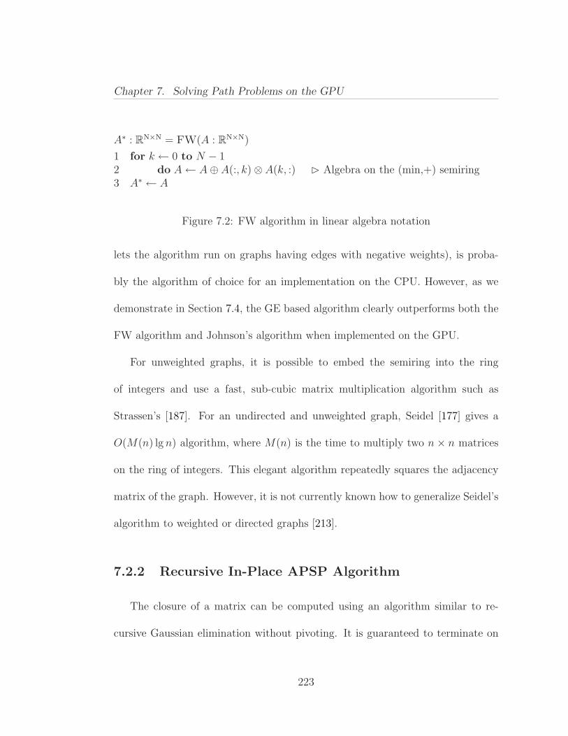
Chapter 7. Solving Path Problems on the GPU
A∗ : RN×N = FW(A : R
N×N)
1 for k ← 0 to N − 12 do A← A⊕ A(:, k)⊗ A(k, :) Algebra on the (min,+) semiring3 A∗ ← A
Figure 7.2: FW algorithm in linear algebra notation
lets the algorithm run on graphs having edges with negative weights), is proba-
bly the algorithm of choice for an implementation on the CPU. However, as we
demonstrate in Section 7.4, the GE based algorithm clearly outperforms both the
FW algorithm and Johnson’s algorithm when implemented on the GPU.
For unweighted graphs, it is possible to embed the semiring into the ring
of integers and use a fast, sub-cubic matrix multiplication algorithm such as
Strassen’s [187]. For an undirected and unweighted graph, Seidel [177] gives a
O(M(n) lg n) algorithm, where M(n) is the time to multiply two n × n matrices
on the ring of integers. This elegant algorithm repeatedly squares the adjacency
matrix of the graph. However, it is not currently known how to generalize Seidel’s
algorithm to weighted or directed graphs [213].
7.2.2 Recursive In-Place APSP Algorithm
The closure of a matrix can be computed using an algorithm similar to re-
cursive Gaussian elimination without pivoting. It is guaranteed to terminate on
223
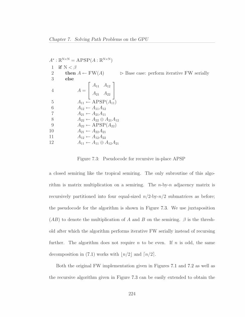
Chapter 7. Solving Path Problems on the GPU
A∗ : RN×N = APSP(A : R
N×N)
1 if N < β2 then A← FW(A) Base case: perform iterative FW serially3 else
4 A =
A11 A12
A21 A22
5 A11 ← APSP(A11)6 A12 ← A11A12
7 A21 ← A21A11
8 A22 ← A22 ⊕ A21A12
9 A22 ← APSP(A22)10 A21 ← A22A21
11 A12 ← A12A22
12 A11 ← A11 ⊕ A12A21
Figure 7.3: Pseudocode for recursive in-place APSP
a closed semiring like the tropical semiring. The only subroutine of this algo-
rithm is matrix multiplication on a semiring. The n-by-n adjacency matrix is
recursively partitioned into four equal-sized n/2-by-n/2 submatrices as before;
the pseudocode for the algorithm is shown in Figure 7.3. We use juxtaposition
(AB) to denote the multiplication of A and B on the semiring. β is the thresh-
old after which the algorithm performs iterative FW serially instead of recursing
further. The algorithm does not require n to be even. If n is odd, the same
decomposition in (7.1) works with ⌊n/2⌋ and ⌈n/2⌉.
Both the original FW implementation given in Figures 7.1 and 7.2 as well as
the recursive algorithm given in Figure 7.3 can be easily extended to obtain the
224
Chapter 7. Solving Path Problems on the GPU
actual minimal paths. In this case, an additional integer matrix Π of predecessor
vertices is maintained. Initially, Π(i, j) ← i for all i. It is updated whenever
a previously unknown path with shorter length is discovered, i.e., Π(i, j) ← k
whenever A(i, k) + A(k, j) < A(i, j) during the computation. As FW and APSP
are essentially performing the same computation, the discovered shortest path is
guaranteed to be a path with minimal length. However, they may find different,
yet equal in length, paths in the presence of multiple shortest paths for a source-
destination pair. This is due to possibly different schedule of path computation.
Recursive formulations of APSP have been presented by many researchers over
the years [71, 158, 196]. The connection to semiring matrix multiplication was
shown by Aho et al. [7], but they did not present a complete algorithm. Ours is
a modified version of the algorithm of Tiskin [196] and R-Kleene algorithm [71].
Especially, the in-place nature of the R-Kleene algorithm helped us avoid expen-
sive global memory to global memory data copying. As the algorithm makes use
of matrix multiplication as a subroutine, it has a much higher data reuse ratio
while having asymptotically the same operation count.
The correctness of the recursive algorithm has been formally proven in various
ways before [71, 158]. Here we present a simpler proof based on algebraic paths.
As in Aho et al. [7], we partition the set of vertices into V1 = v1, ..., vn/2 and
V2 = vn/2+1, ..., vn. Submatrix A11 represents the edges within V1, submatrix
225
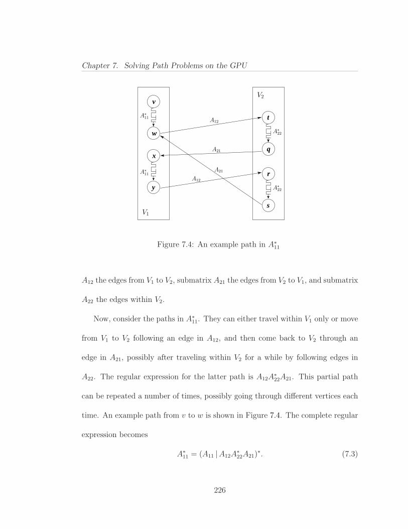
Chapter 7. Solving Path Problems on the GPU
w
v
x
t
q
y
r
sV1
A∗11
V2
A∗11
A12
A21
A21
A12
A∗22
A∗22
Figure 7.4: An example path in A∗11
A12 the edges from V1 to V2, submatrix A21 the edges from V2 to V1, and submatrix
A22 the edges within V2.
Now, consider the paths in A∗11. They can either travel within V1 only or move
from V1 to V2 following an edge in A12, and then come back to V2 through an
edge in A21, possibly after traveling within V2 for a while by following edges in
A22. The regular expression for the latter path is A12A∗22A21. This partial path
can be repeated a number of times, possibly going through different vertices each
time. An example path from v to w is shown in Figure 7.4. The complete regular
expression becomes
A∗11 = (A11 |A12A
∗22A21)
∗. (7.3)
226
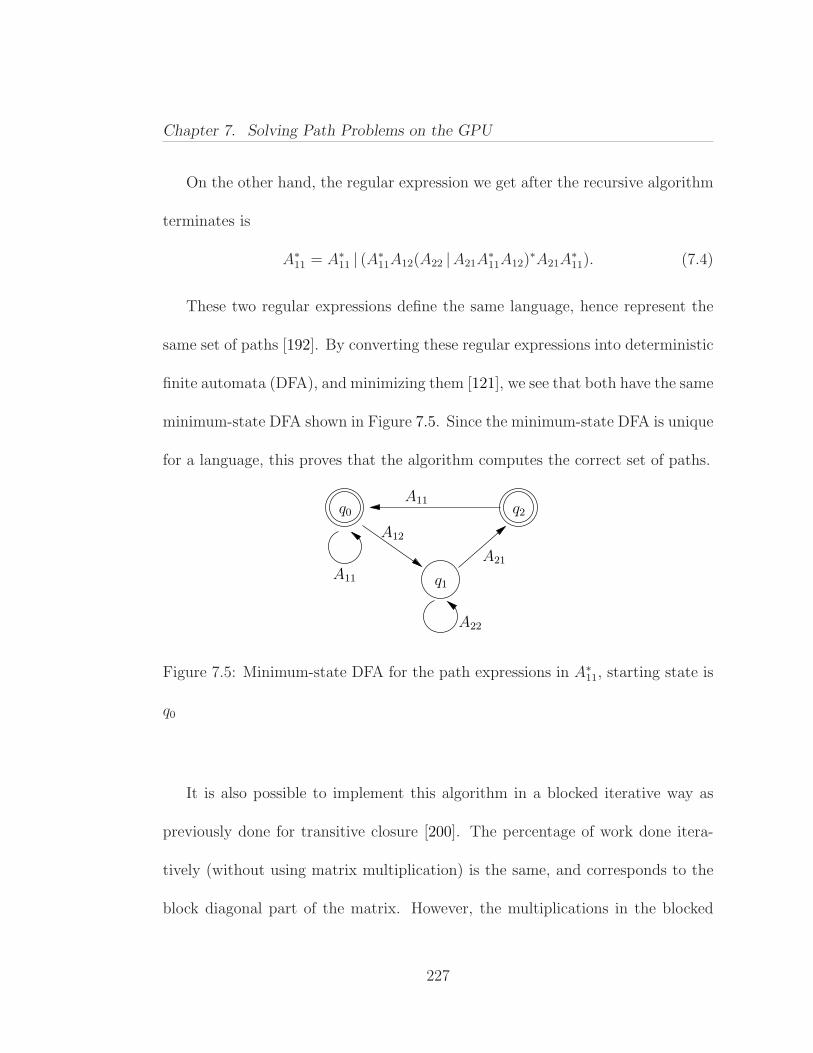
Chapter 7. Solving Path Problems on the GPU
On the other hand, the regular expression we get after the recursive algorithm
terminates is
A∗11 = A∗
11 | (A∗11A12(A22 |A21A
∗11A12)
∗A21A∗11). (7.4)
These two regular expressions define the same language, hence represent the
same set of paths [192]. By converting these regular expressions into deterministic
finite automata (DFA), and minimizing them [121], we see that both have the same
minimum-state DFA shown in Figure 7.5. Since the minimum-state DFA is unique
for a language, this proves that the algorithm computes the correct set of paths.
q1A11
A12
A21
A22
A11q0 q2
Figure 7.5: Minimum-state DFA for the path expressions in A∗11, starting state is
q0
It is also possible to implement this algorithm in a blocked iterative way as
previously done for transitive closure [200]. The percentage of work done itera-
tively (without using matrix multiplication) is the same, and corresponds to the
block diagonal part of the matrix. However, the multiplications in the blocked
227
Chapter 7. Solving Path Problems on the GPU
algorithm are always between matrices of size B × B, where B is the blocking
factor. This is potentially a limiting factor on GPUs because multiplication tends
to get drastically faster as matrices get bigger (less than 20 GFlops/s when N=64
versus 200 GFlops/s when N=1024) [204]. With the recursive formulation, on the
other hand, more work can be done during multiplication of large matrices.
Furthermore, the recursive algorithm does fewer kernel launches than the block
iterative one. The block iterative algorithm launches O((N/B)3) kernels for matrix
multiplications and O(N/B) kernels for computing closures of B × B blocks on
the diagonal. On the other hand, at each level of the recursion tree, the recursive
algorithm launches 6 kernels for matrix multiplications, and does 2 recursive calls.
This makes a total of only O(N/B) kernel launches because the height of the
recursion tree is lg (N/B), and the number of kernel launches doubles at each
level (6, 12, 24, ..., 6(N/B)). The O((N/B)2) factor of improvement can be quite
significant, as kernel launches incur significant overhead in CUDA.
One important feature of our implementation is that it is performed in place,
overwriting the input with the output without constraining the order of loops
in the matrix multiplication. For the matrix multiply-add operations A22 ←
A22 ⊕ A21A12 and A11 ← A11 ⊕ A12A21, there are no issues of correctness. How-
ever, for other multiplications of the form B ← BA or B ← AB, the order of
evaluation (whether it is an ijk loop or an kji loop) matters on a general semiring.
228
Chapter 7. Solving Path Problems on the GPU
This is because updating the output automatically updates the input, and the al-
gorithm will now use a different input for the rest of the computation. As proved
by D’Alberto and Nicolau [71], this is not a problem as long as the semiring is
idempotent and A is a closure. The intuition is that if the algorithm prematurely
overwrites its input, this just makes the algorithm find shortest paths quicker. In
other words, it speeds up the information dissemination, but the correctness is
preserved thanks to idempotence.
Note that four of the six multiplications at any level of the recursion tree are
of the form B ← BA or B ← AB. In other words, they perform multiply instead
of multiply-add operations. Using B ← B + BA or B ← B + AB would be
equally correct, but unnecessary. Remember that the cost of staying in a vertex is
zero, i.e., A(i, i) = 0. Consider B ← AB: If B contains a path vi ⇒ vj before the
operation, AB generates a cost-equivalent path vi ⇒ vi ⇒ vj and safely overwrites
B.
7.3 GPU Computing Model with CUDA
More and more applications that traditionally run on the CPU are now being
reimplemented to run on the GPU, a technique called general-purpose computing
on graphics processing units (GPGPU). Both Nvidia and AMD offer programming
229
Chapter 7. Solving Path Problems on the GPU
interfaces for making GPGPU accessible to programmers who are not experts in
computer graphics [1, 2]. Nvidia’s Compute Unified Device Architecture (Cuda)
offers a higher level C-like API, whereas AMD’s Close-to-Metal (CTM) allows the
programmers to access lower levels of hardware. As opposed to CTM, the Cuda
platform is unified in the sense that it has no architectural division for vertex and
pixel processing.
7.3.1 GPU Programming
The new generation of GPUs are basically multithreaded stream processors.
They offer tremendous amounts of bandwidth and single-precision floating point
arithmetic computation rates. In stream processing, a single data parallel func-
tion (kernel) is executed on a stream of data, and that is exactly how the Cuda
programming model works. A Cuda program is composed of two parts: A host
(CPU) code that makes kernel calls, and a device (GPU) code that actually im-
plements the kernel. The host code is conceptually a serial C program, but the
device code should be massively parallel in order to harness the power of the GPU.
The fundamental building block of Nvidia 8 and 9 series is the streaming
multiprocessors (SMs), sometimes called the GPU chips. Each SM consists of 8
streaming processors (cores), but only one instruction fetch/decode unit. This
implies that all 8 cores must simultaneously execute the same instruction. This
230
Chapter 7. Solving Path Problems on the GPU
is why divergence in the device code should be avoided as much as possible. The
memory hierarchy consists of multiple levels. Each SM has 8192 registers and
16KB on-chip shared memory, which is as fast as registers provided that bank
conflicts are avoided. A high-latency (200-300 cycles) off-chip global memory
provides the main storage for the application on the GPU. Part of the off-chip
memory, called the local memory, is used for storing variables that are spilled from
registers.
A kernel is executed by many threads on the GPU. These threads are organized
as a grid of thread blocks, which are batches of threads that can cooperate/com-
municate through on-chip shared memory and synchronize their execution. Each
thread block is executed by only one SM, but each SM can execute multiple thread
blocks simultaneously.
The main scheduling unit in Cuda is a warp, a group of 32 threads from
the same thread block. All threads in a warp execute the same instruction, and
execution of an arithmetic instruction for the whole warp takes 4 clock cycles.
The number of active warps in a block is an important factor in tolerating global
memory access latency.
231

Chapter 7. Solving Path Problems on the GPU
7.3.2 Experiences and Observations
Some limitations exist for the device code. For example, recursion and static
variables are not allowed. These limitations do not apply to the host code, as
it is just a regular C code running on the CPU. In fact, recursion in the host
code is a powerful technique, since it naturally separates the recursion stack from
the floating-point intensive part of the program. Although recursive divide-and-
conquer algorithms are naturally cache efficient [114], they have traditionally not
achieved their full performance due to the overheads associated with recursion.
We do not have such a limitation with CUDA because the recursion stack, which
is on the CPU, does not interfere with the kernel code on the GPU.
Code optimization on a GPU is a tedious job with many pitfalls. Performance
on a GPU is often more fragile than performance on a CPU. It has been observed
that small changes can cause huge effects on the performance [170]. For example,
in the optimized GEMM routine of Volkov [204], each thread block is 16× 4 and
each thread uses 32 registers. This allows 8192/32 = 256 threads and 256/64 = 4
thread blocks can simultaneously be active on each SM. As there are two warps
per thread block and it takes 4 cycles to execute an instruction for the whole warp,
a latency of 8×4 = 32 cycles can be completely hidden. In the case that an extra
variable is required, the compiler can either choose to spill it out to local memory
and keep the register count intact, or increase the register usage per thread by
232

Chapter 7. Solving Path Problems on the GPU
one. In the latter case, the number of active thread blocks decreases to 3. This
introduces a 25% reduction in parallelism, but the former option may perform
worse if the kernel has few instructions because access to a local variable will
introduce one-time extra latency of 200-300 cycles. Whichever option is chosen, it
is obvious that performance is fragile: by just adding one extra line, it is possible
to drastically slow down the computation.
Another pitfall awaiting the programmer is bandwidth optimizations. In Cuda,
peak bandwidth can only be achieved through memory coalescing, i.e., by making
consecutively numbered threads access consecutive memory locations. One can
heavily underutilize the GPU bandwidth by not paying attention to memory co-
alescing. However, the way memory coalescing works is quite counter-intuitive to
a multicore programmer. Assume that one wants to scan a 16×N matrix stored
in row-major order. On an SMP system with 16 cores, the most bandwidth-
friendly way is to let each processor scan a different row of the matrix; in this
case, each processor makes at most N/B cache misses, which is optimal. On an
Nvidia GPU, on the other hand, this will create multiple memory accesses per
warp since these threads do not access contiguous range of memory addresses.
An example with N = 8 is shown in Figure 7.6. However, if the matrix were
stored in column-major order, having each thread scan a different row would be
optimal on an Nvidia GPU. This is because memory accesses at each step would
233
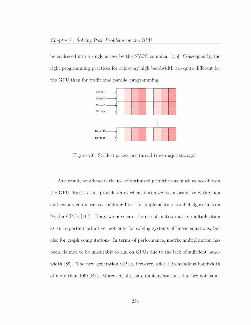
Chapter 7. Solving Path Problems on the GPU
be coalesced into a single access by the NVCC compiler [155]. Consequently, the
right programming practices for achieving high bandwidth are quite different for
the GPU than for traditional parallel programming.
Thread 16
Thread 1
Thread 2
Thread 3
Thread 4
Thread 15
Figure 7.6: Stride-1 access per thread (row-major storage)
As a result, we advocate the use of optimized primitives as much as possible on
the GPU. Harris et al. provide an excellent optimized scan primitive with Cuda
and encourage its use as a building block for implementing parallel algorithms on
Nvidia GPUs [117]. Here, we advocate the use of matrix-matrix multiplication
as an important primitive, not only for solving systems of linear equations, but
also for graph computations. In terms of performance, matrix multiplication has
been claimed to be unsuitable to run on GPUs due to the lack of sufficient band-
width [89]. The new generation GPUs, however, offer a tremendous bandwidth
of more than 100 GB/s. Moreover, alternate implementations that are not band-
234
Chapter 7. Solving Path Problems on the GPU
width bound achieved close to peak performance [204]. It would be wise to take
advantage of such an efficient primitive whenever possible.
7.4 Implementation and Experimentation
7.4.1 Experimental Platforms
We ran our GPU code on an Nvidia GeForce 8800 Ultra with Cuda SDK
1.1 and GCC version 4.1. The graphics card driver installed in our system is
Nvidia Unix x86 64 kernel module 169.09. The GeForce 8800 Ultra has 768 MB
DRAM, a core clock of 612 MHz, a stream processor clock of 1.5 GHz, a memory
clock of 1080 MHz, and an impressive bandwidth of 103.7 GB/s. It consists of
16 SMs, each containing 8 cores, making up a total of 128 cores. Each core
can perform a multiply-add operation in a single cycle, which accounts for two
floating-point operations (Flops). Therefore, it offers a peak multiply-add rate of
2× 1.5× 128 = 384 GFlops/s (not counting the extra MUL operation that cores
can issue only under certain circumstances).
For comparison, we ran our CPU experiments in three different settings:
1. Serial C++ code on Intel Core 2 Duo T2400 1.83 Ghz with 1 GB RAM
running Windows XP. Two cores share a 2 MB L2 Cache.
235
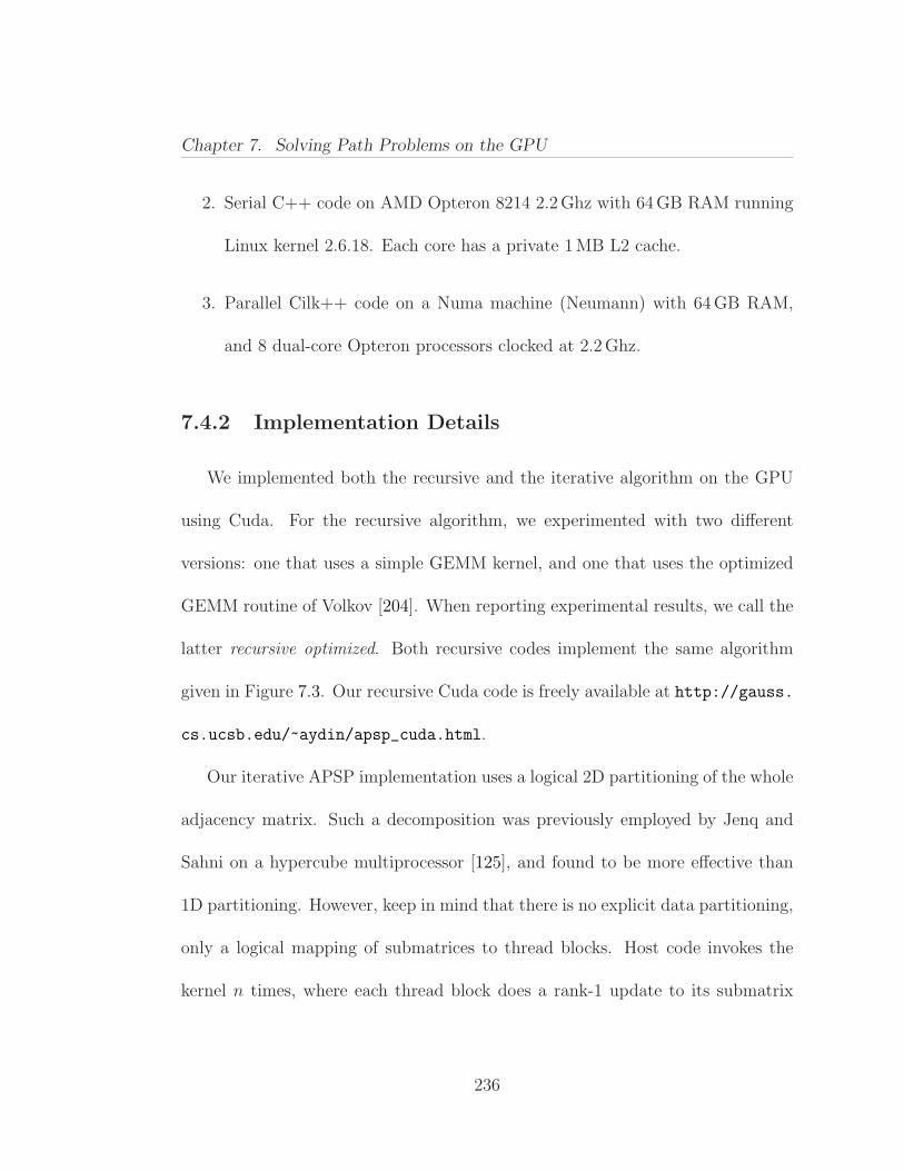
Chapter 7. Solving Path Problems on the GPU
2. Serial C++ code on AMD Opteron 8214 2.2 Ghz with 64 GB RAM running
Linux kernel 2.6.18. Each core has a private 1 MB L2 cache.
3. Parallel Cilk++ code on a Numa machine (Neumann) with 64 GB RAM,
and 8 dual-core Opteron processors clocked at 2.2 Ghz.
7.4.2 Implementation Details
We implemented both the recursive and the iterative algorithm on the GPU
using Cuda. For the recursive algorithm, we experimented with two different
versions: one that uses a simple GEMM kernel, and one that uses the optimized
GEMM routine of Volkov [204]. When reporting experimental results, we call the
latter recursive optimized. Both recursive codes implement the same algorithm
given in Figure 7.3. Our recursive Cuda code is freely available at http://gauss.
cs.ucsb.edu/~aydin/apsp_cuda.html.
Our iterative APSP implementation uses a logical 2D partitioning of the whole
adjacency matrix. Such a decomposition was previously employed by Jenq and
Sahni on a hypercube multiprocessor [125], and found to be more effective than
1D partitioning. However, keep in mind that there is no explicit data partitioning,
only a logical mapping of submatrices to thread blocks. Host code invokes the
kernel n times, where each thread block does a rank-1 update to its submatrix
236
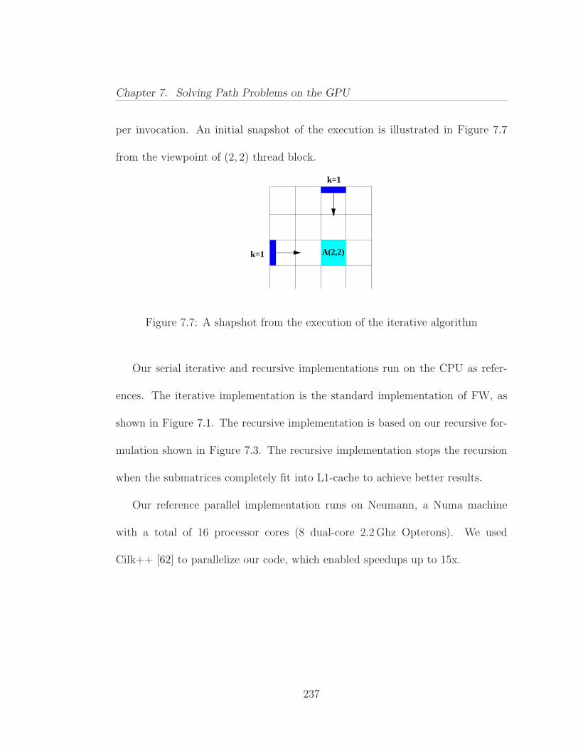
Chapter 7. Solving Path Problems on the GPU
per invocation. An initial snapshot of the execution is illustrated in Figure 7.7
from the viewpoint of (2, 2) thread block.
k=1
k=1
A(2,2)
Figure 7.7: A shapshot from the execution of the iterative algorithm
Our serial iterative and recursive implementations run on the CPU as refer-
ences. The iterative implementation is the standard implementation of FW, as
shown in Figure 7.1. The recursive implementation is based on our recursive for-
mulation shown in Figure 7.3. The recursive implementation stops the recursion
when the submatrices completely fit into L1-cache to achieve better results.
Our reference parallel implementation runs on Neumann, a Numa machine
with a total of 16 processor cores (8 dual-core 2.2 Ghz Opterons). We used
Cilk++ [62] to parallelize our code, which enabled speedups up to 15x.
237
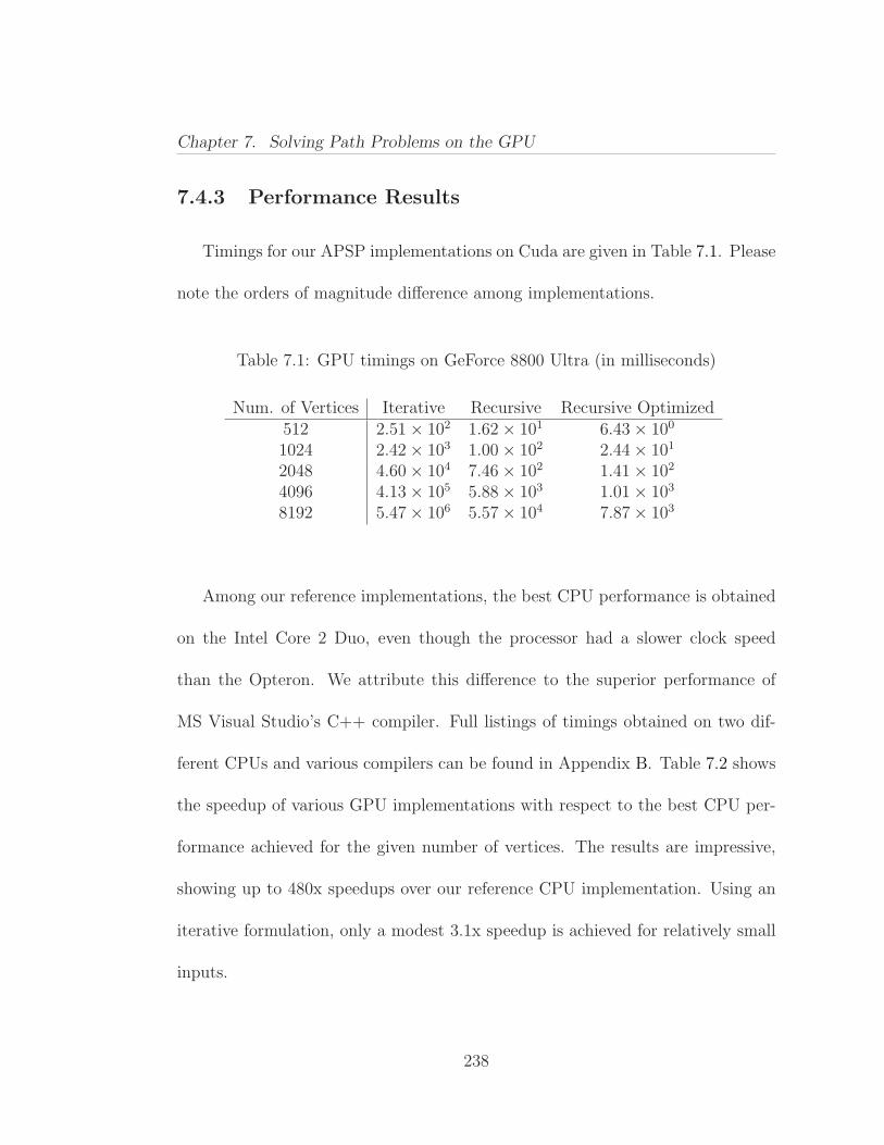
Chapter 7. Solving Path Problems on the GPU
7.4.3 Performance Results
Timings for our APSP implementations on Cuda are given in Table 7.1. Please
note the orders of magnitude difference among implementations.
Table 7.1: GPU timings on GeForce 8800 Ultra (in milliseconds)
Num. of Vertices Iterative Recursive Recursive Optimized512 2.51× 10² 1.62× 101 6.43× 100
1024 2.42× 10³ 1.00× 10² 2.44× 101
2048 4.60× 10⁴ 7.46× 10² 1.41× 10²
4096 4.13× 10⁵ 5.88× 10³ 1.01× 10³
8192 5.47× 10⁶ 5.57× 10⁴ 7.87× 10³
Among our reference implementations, the best CPU performance is obtained
on the Intel Core 2 Duo, even though the processor had a slower clock speed
than the Opteron. We attribute this difference to the superior performance of
MS Visual Studio’s C++ compiler. Full listings of timings obtained on two dif-
ferent CPUs and various compilers can be found in Appendix B. Table 7.2 shows
the speedup of various GPU implementations with respect to the best CPU per-
formance achieved for the given number of vertices. The results are impressive,
showing up to 480x speedups over our reference CPU implementation. Using an
iterative formulation, only a modest 3.1x speedup is achieved for relatively small
inputs.
238
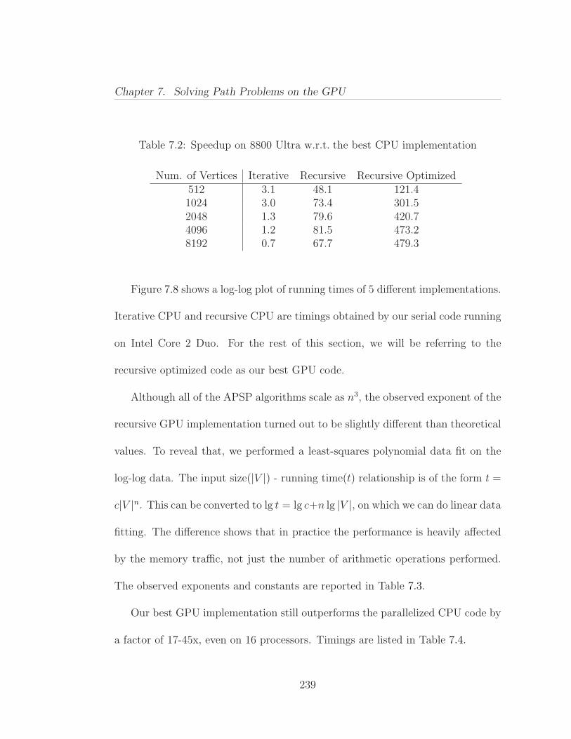
Chapter 7. Solving Path Problems on the GPU
Table 7.2: Speedup on 8800 Ultra w.r.t. the best CPU implementation
Num. of Vertices Iterative Recursive Recursive Optimized512 3.1 48.1 121.41024 3.0 73.4 301.52048 1.3 79.6 420.74096 1.2 81.5 473.28192 0.7 67.7 479.3
Figure 7.8 shows a log-log plot of running times of 5 different implementations.
Iterative CPU and recursive CPU are timings obtained by our serial code running
on Intel Core 2 Duo. For the rest of this section, we will be referring to the
recursive optimized code as our best GPU code.
Although all of the APSP algorithms scale as n3, the observed exponent of the
recursive GPU implementation turned out to be slightly different than theoretical
values. To reveal that, we performed a least-squares polynomial data fit on the
log-log data. The input size(|V |) - running time(t) relationship is of the form t =
c|V |n. This can be converted to lg t = lg c+n lg |V |, on which we can do linear data
fitting. The difference shows that in practice the performance is heavily affected
by the memory traffic, not just the number of arithmetic operations performed.
The observed exponents and constants are reported in Table 7.3.
Our best GPU implementation still outperforms the parallelized CPU code by
a factor of 17-45x, even on 16 processors. Timings are listed in Table 7.4.
239

Chapter 7. Solving Path Problems on the GPU
Table 7.3: Observed exponents and constants for the asymptotic behaviour of our
APSP implementations with increasing problem size
t = c|V |n CPU (Intel Core 2 Duo) GPU (GeForce 8800 Ultra)
Iterative Recursive Iterative Recursive Recur. Optimized
Exponent (n) 3.02 3.23 3.62 2.94 2.59Constant (c) 5.5× 10⁻⁶ 1.4× 10⁻⁶ 3.6× 10⁻⁸ 1.5× 10⁻⁷ 4.7× 10⁻⁷
Table 7.4: Performance comparison of our best (optimized recursive) GPU imple-
mentation with parallel Cilk++ code running on Neumann, using all 16 cores
Num. of Vertices Best GPU (secs) Parallel CPU (secs) GPU Speedup512 0.00643 0.113 17.5×1024 0.0244 0.708 29×2048 0.141 5.146 36.5×4096 1.01 40.36 40×8192 7.87 354.9 45×
240

Chapter 7. Solving Path Problems on the GPU
1
10
100
1000
10000
100000
1e+06
512 1024 2048 4096 8192
Tim
e (m
illis
econ
ds)
Number of Vertices
Iterative CPURecursive CPU
Iterative GPURecursive GPU
Recursive Optimized GPU
Figure 7.8: Log-log plot of absolute running times
7.4.4 Comparison with Earlier Performance Results
We compare the performance of our code with two previously reported results.
One is an automatically generated, highly optimized serial program running on a
3.6 Ghz Pentium 4 CPU [115]. The other is due to Harish and Narayanan on a
GPU platform very similar to ours [116]. Our GeForce 8800 Ultra is slightly faster
than the GeForce 8800 GTX used by Harish and Narayanan, so we underclocked
our GPU to allow a direct comparison in terms of absolute values.
On the GPU, Harish and Narayanan implemented two variants of APSP: one
that uses the FW algorithm and one that runs Dijkstra’s single source shortest
paths (SSSP) algorithm for every vertex. For sparse graphs with m = O(n),
241

Chapter 7. Solving Path Problems on the GPU
100
1000
10000
100000
1024 2048 4096 8192
Tim
e (m
illis
econ
ds)
Number of Vertices
Optimized Recursive (GTX)H&N APSP (GTX)H&N SSSP (GTX)
Figure 7.9: Comparison of different GPU implementations on 8800 GTX settings
the latter is theoretically faster than both the FW algorithm and our recursive
formulation in the classical RAM model of computation [7]. It runs in O(n2 lg n+
nm) time using Fibonacci heaps [95].
As seen in Figure 7.9, our recursive implementation significantly outperforms
both their FW implementation (H&N APSP) and Dijkstra based implementa-
tion (H&N SSSP) when implemented on a GPU. The running times for the H&N
SSSP code are observed for randomly generated Erdos-Renyi graphs with an av-
erage vertex degree of 6. The running times of the other two implementations are
not sensitive to sparsity. When timing our algorithm, we underclocked our GPU’s
clocks down to the speed of 8800 GTX for a head-to-head comparison. Due to the
242
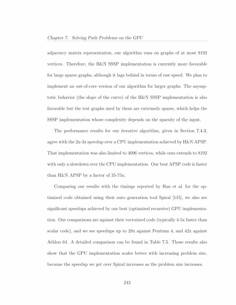
Chapter 7. Solving Path Problems on the GPU
adjacency matrix representation, our algorithm runs on graphs of at most 8192
vertices. Therefore, the H&N SSSP implementation is currently more favorable
for large sparse graphs, although it lags behind in terms of raw speed. We plan to
implement an out-of-core version of our algorithm for larger graphs. The asymp-
totic behavior (the slope of the curve) of the H&N SSSP implementation is also
favorable but the test graphs used by them are extremely sparse, which helps the
SSSP implementation whose complexity depends on the sparsity of the input.
The performance results for our iterative algorithm, given in Section 7.4.3,
agree with the 2x-3x speedup over a CPU implementation achieved by H&N APSP.
That implementation was also limited to 4096 vertices, while ours extends to 8192
with only a slowdown over the CPU implementation. Our best APSP code is faster
than H&N APSP by a factor of 35-75x.
Comparing our results with the timings reported by Han et al. for the op-
timized code obtained using their auto generation tool Spiral [115], we also see
significant speedups achieved by our best (optimized recursive) GPU implementa-
tion. Our comparisons are against their vectorized code (typically 4-5x faster than
scalar code), and we see speedups up to 28x against Pentium 4, and 42x against
Athlon 64. A detailed comparison can be found in Table 7.5. Those results also
show that the GPU implementation scales better with increasing problem size,
because the speedup we get over Spiral increases as the problem size increases.
243

Chapter 7. Solving Path Problems on the GPU
Table 7.5: Comparisons of our best GPU implementation with the timings re-
ported for Han et al. ’s auto generation tool Spiral
Num. of VerticesGFlops/s Speedup of GeForce
GeForce 8800 Pentium 4 Athlon 64 Pentium 4 Athlon 64512 38.6 5.08 3.17 7.6x 12.2x1024 82.0 5.00 2.77 16.4x 29.6x2048 113.5 4.78 2.73 23.7x 41.6x4096 126.7 4.47 2.96 28.3x 42.8x
7.4.5 Scalability and Resource Usage
In this section, we try to identify the bottlenecks in our implementation in
terms of resource usage and scalability. By using the NVIDIA Coolbits utility,
we tweaked the frequencies of both the GPU core clock and the memory clock.
The results reveal that our recursive implementation is not limited by the mem-
ory bandwidth to global GPU DRAM. For this implementation, the timings and
GFlops/s rates with different clock rates are given in Table 7.6. When the mem-
ory clock is fixed, the slowdown of the computation closely tracks the slowdown
of the GPU core clock (0-50% with increments of 12.5%). On the other hand,
when the GPU core clock is fixed, little slowdown is observed when we underclock
the memory clock. Coolbits reported the default clock speeds of 8800 Ultra as
648 Mhz for cores, and 1152 Mhz for memory, which are slightly different than the
values reported in NVIDIA factsheets.
244
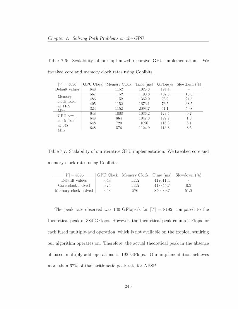
Chapter 7. Solving Path Problems on the GPU
Table 7.6: Scalability of our optimized recursive GPU implementation. We
tweaked core and memory clock rates using Coolbits.
|V | = 4096 GPU Clock Memory Clock Time (ms) GFlops/s Slowdown (%)Default values 648 1152 1028.3 124.4 -
Memoryclock fixedat 1152Mhz
567 1152 1190.8 107.5 13.6486 1152 1362.9 93.9 24.5405 1152 1673.1 76.5 38.5324 1152 2093.7 61.1 50.8
GPU coreclock fixedat 648Mhz
648 1008 1036.2 123.5 0.7648 864 1047.3 122.2 1.8648 720 1096 116.8 6.1648 576 1124.9 113.8 8.5
Table 7.7: Scalability of our iterative GPU implementation. We tweaked core and
memory clock rates using Coolbits.
|V | = 4096 GPU Clock Memory Clock Time (ms) Slowdown (%)Default values 648 1152 417611.4 -
Core clock halved 324 1152 418845.7 0.3Memory clock halved 648 576 856689.7 51.2
The peak rate observed was 130 GFlops/s for |V | = 8192, compared to the
theoretical peak of 384 GFlops. However, the theoretical peak counts 2 Flops for
each fused multiply-add operation, which is not available on the tropical semiring
our algorithm operates on. Therefore, the actual theoretical peak in the absence
of fused multiply-add operations is 192 GFlops. Our implementation achieves
more than 67% of that arithmetic peak rate for APSP.
245
Chapter 7. Solving Path Problems on the GPU
The iterative implementation, on the other hand, is observed to be completely
bandwidth bound. Even when the GPU cores are underclocked to half, no slow-
down was observed. Underclocking the memory to half, however, slowed down the
computation by exactly a factor of two. Exact timings can be seen in Figure 7.7.
We conclude that the iterative formulation is putting too much stress on GPU
memory bandwidth, consequently not harnessing the available computation power
of the GPU. This is indeed expected, because the iterative formulation accesses
O(n2) data and does O(n2) work in every iteration. The recursive algorithm, on
the other hand, does almost all of its work in matrix multiplications, which ac-
cess O(n2) data for doing O(n3) work. Therefore, it clearly has better locality of
reference.
As it was not possible to disable a subset of GPU cores in the NVIDIA 8800,
we do not report any scalability results with increasing number of processors.
7.4.6 Power and Economic Efficiency
Power efficiency is becoming an important consideration when comparing dif-
ferent architectures [90]. The Green500 list ranks supercomputers according to
their Flops/Watts×sec (or Flops/Joule) ratio. In this section, we compare the
power efficiency of different architectures for the APSP problem, using power
specs of the manufacturer’s equipment (in Thermal Watts)
246
Chapter 7. Solving Path Problems on the GPU
Nvidia reports a peak power consumption of 175 Watts for its GeForce 8800
Ultra video card. Our dual-core Opteron (model number 8214) is reported to
consume a peak power of 95 Watts, but we are using only a single core of it during
serial computation. The machines used in the reported timings of automatically
tuned CPU implementations are Pentium 4 (model number 560) and Athlon 64
(model 4000+). They consume 115 and 89 Watts, respectively. The Intel Core
Duo T2400, the most power efficient CPU in this comparison, has a maximum
power consumption of only 31 Watts even when both cores are active.
This comparative study should be considered very preliminary, because we are
not running the same code in every architecture. The GPU code is assumed to
use 175 + 95/2 = 222.5 Watts as it also uses one of the CPU cores to assist the
computation. This is also a rough estimate as it is likely that when one core is
idle, the whole processor’s power consumption is more than half of its maximum.
However, our rationale is that it is possible to use the other core to perform the
same computation on a different input.
The results, outlined in Table 7.8, show that the Nvidia Cuda implementa-
tion is not only powerful, but also efficient. The closest competitor is the auto
generated Spiral [115] code that runs on Pentium 4. Note that Pentium 4 is not
a particularly power efficient processor. Therefore, it is plausible that an auto
generated code on more power efficient hardware would get closer to the efficiency
247

Chapter 7. Solving Path Problems on the GPU
Table 7.8: Efficiency comparison of different architectures (running various codes),
values in MFlops/Watts×sec (or equivalently MFlops/Joule)
|V | Nvidia GPU Athlon Pentium 4 Core 2 Duo Neumann (Opteron)
Best Cuda code Spiral Code Reference FW Cilk++ (p=16)
512 173 35.6 44.1 19.1 2.91024 368 31.1 43.7 17.4 3.72048 510 30.6 41.5 17.3 4.14096 569 33.2 38.8 17.2 4.2
of the GPU. A couple of factors contribute to the inefficiency of Neumann. The
most important one being that the Opterons we use are not high-efficiency (HE)
versions, but rather high-performance Opterons. A single Opteron core in Neu-
mann consumes more than three times the power that is consumed by Core 2
Duo, while still giving worse performance in this particular problem.
Looking at the timings are listed in Table 7.4, the economic efficiency of the
GPU is also clear. At the time of writing, the processors of our 8-way Opteron
server is priced about 7x the price of Nvidia GPUs we have been using. Given
that the GPU implementation runs about 17-45x faster, we see Flops/Dollar ratio
of the GPU is up to 119-315x better than an 8-way server. These statements are
by no means conclusive as they are based on APSP performance only.
248
Chapter 7. Solving Path Problems on the GPU
7.5 Conclusions and Future Work
We have considered the efficient implementation of Gaussian elimination based
algorithms on the GPU. Choosing the right algorithm that efficiently maps to the
underlying hardware has always been important in high-performance computing.
Our work shows that it is even more important when the hardware in question
is a GPU. Our proof-of-concept implementation runs more than two orders of
magnitude faster than a simple porting of the most popular algorithm to the
GPU. The key to performance was to choose an algorithm that has good locality
of reference and makes the most use of optimized kernels.
We made extensive comparisons with our reference implementations on single
processor and shared memory multiprocessor systems, as well as with previously
reported results obtained on various CPUs and GPUs. Future work includes
identifying and implementing crucial kernels that are likely to speed up a large
class of applications. Specifically, we are working on implementing an efficient
sparse matrix-matrix multiplication algorithm on the GPU, which is to be used
as a building block for many graph algorithms [48, 49].
249
Chapter 7. Solving Path Problems on the GPU
Acknowledgments
We acknowledge the kind permission of Charles Leiserson and CilkArts to use
an alpha release of the Cilk++ language. We also thank P.J.Narayanan and Pawan
Harish for providing us the exact timings from their experiments. Sivan Toledo
helped us improve the presentation of the paper with various comments. Thanks
to Fenglin Liao and Arda Atali for their help during the initial implementation
on Cuda. Finally, we would like to thank three anonymous reviewers for their
constructive comments that improved the presentation.
250
Chapter 8
Conclusions and FutureDirections
Our Sultan told us to come, here we came.
Mercan Dede
This thesis aims to provide a solution to the problem of graph analysis and data
mining, especially for tightly-coupled computations. It proposes a scalable high-
performance library along with a clear direction on the discovery and refinement
of novel algorithms on this subject.
Graph computations are pervasive in sciences and it is our view that they will
become more so in the future. We showed that carefully chosen and implemented
primitive operations are key to high performance. This thesis specifically focused
on linear algebraic primitives. This is not to claim that linear algebraic primi-
tives are the only primitives needed to perform graph analysis and data mining;
they are, however, general enough to be widely useful and compact enough to be
implemented in a reasonable time frame.
251
Chapter 8. Conclusions and Future Directions
This work will hopefully become a significant addition to the diversity of com-
binatorial scientific computing, with its unique emphasis on solving combinatorial
problems using matrix methods. The contents of this thesis fall into the areas of
graph algorithms, network science, parallel computing, sparse matrix algorithms,
software engineering, and performance evaluation. Its main goal is, however, en-
abling scientific applications by facilitating large scale parallel graph analysis.
The primary applications of this thesis are in computational domain sciences such
as biology, ecology, chemistry, and cosmology. I hope this work will modestly
contribute to the increasing interaction between domain sciences and computer
sciences. As tool builders for domain sciences, computer scientists face a challeng-
ing task imposed by increasingly complex computer architectures.
This work can be extended in four main directions:
(1) Support for higher dimensional data in the combinatorial BLAS.
The first class citizens of the combinatorial BLAS are (sparse) matrices. Some
emerging applications need a higher dimensional representation of data, where
matrices are often replaced by tensors. Similarly, a more expressive way of mod-
eling the data is to use hypergraphs, which are generalizations of graphs where
the interactions among vertices is not restricted to be pairwise. Although a rect-
angular sparse matrix is a natural representation of an hypergraph, the right set
252

Chapter 8. Conclusions and Future Directions
of primitives for computations on hypergraphs is not clear at the moment. I will
be exploring these two extensions to provide a more complete library.
(2) Hybrid MPI and shared-memory support in the combinatorial BLAS.
Looking at the recently deployed systems targeting text and data mining,
such as the Petascale Data Analysis Facility of SDSC’s Triton resource, we see
that a small number of shared memory nodes having large numbers of cores are
connected to provide the fastest exploration of large data sets. Therefore, intra-
node performance is at least as important as inter-node communication. Even
though the current design of the algorithms in the combinatorial BLAS is moti-
vated by distributed-memory systems, it would perform well in shared memory
too, as it avoids hot spots and load imbalances by ensuring proper work distribu-
tion among processors. Still, algorithms specifically designed for shared-memory
systems and CMPs often outperform distributed-memory algorithms running on
shared memory. I plan to extend our work on compressed sparse blocks beyond
sparse matrix-vector products and incorporate it into the combinatorial BLAS
to achieve better performance on those hybrid architectures that require both
inter-node and intra-node parallelism.
(3) Novel algorithm development for graph and data mining.
253

Chapter 8. Conclusions and Future Directions
Many popular algorithms for graph analysis and data mining are either inexact
or they have not been proven optimal. For example, it is debatable if betweenness
centrality is really the right measure of importance in social networks or if the
higher-order SVD and related decompositions are the right methods for revealing
the hidden properties of higher order data sets. Furthermore, even well-defined
applications frequently need alternative algorithms due to scaling problems that
occur with ever growing data. For example, Chen and Saad [57] found that the
Lanczos algorithm can be a more efficient alternative to the truncated SVD for
dimensionality reduction. Since this algorithm requires only sparse matrix-vector
and matrix-transpose vector products, a highly-parallel version is readily available
by extending our work on compressed sparse blocks.
(4) Usage of different metrics, such as energy and cost efficiency.
So far, high performance computing has solely focused on the performance
aspect. This work, except for the preliminary cost and energy analysis for the all-
pairs shortest-paths problem in Chapter 7, is no exception. Our primary metric of
success was time to solution. However, recent trends suggest that power and mon-
etary costs of systems are exceeding what we will be able to afford [24]. Almost
all aspects of computing, including software, architectures, and algorithms, need
to be rethought with energy and cost efficiency in mind. Comparisons of different
254

Chapter 8. Conclusions and Future Directions
graph libraries should be performed with these metrics in mind. These compar-
isons will also guide the healthy evolution of architectures for graph problems,
since different libraries run on different architectures.
255
Bibliography
[1] AMD Stream Computing. http://ati.amd.com/technology/
streamcomputing.
[2] NVIDIA CUDA. http://www.nvidia.com/cuda.
[3] 23rd IEEE International Symposium on Parallel and Distributed Processing,IPDPS 2009, Rome, Italy, May 23-29, 2009. IEEE, 2009.
[4] M. Adams and J. W. Demmel. Parallel multigrid solver for 3d unstructuredfinite element problems. In Supercomputing ’99: Proceedings of the 1999ACM/IEEE conference on Supercomputing, page 27, New York, NY, USA,1999. ACM.
[5] M. D. Adams and D. S. Wise. Seven at one stroke: results from a cache-oblivious paradigm for scalable matrix algorithms. In MSPC ’06: Proceed-ings of the 2006 workshop on Memory system performance and correctness,pages 41–50, New York, NY, USA, 2006. ACM.
[6] A. Aggarwal and J. S. Vitter. The input/output complexity of sorting andrelated problems. Communications of the ACM, 31(9):1116–1127, 1988.
[7] A. V. Aho, J. E. Hopcroft, and J. D. Ullman. The Design and Analysis ofComputer Algorithms. Addison-Wesley Longman, Boston, MA, USA, 1974.
[8] D. Ajwani, U. Meyer, and V. Osipov. Improved external memory bfs imple-mentation, 2007.
[9] Allinea Software Ltd., Warwick, UK. DDT Software and Users Guide, 2009.Available from http://www.allinea.com/.
[10] G. Almasi, C. Cascaval, J. G. Casta nos, M. Denneau, D. Lieber, J. E.Moreira, and H. S. Warren, Jr. Dissecting cyclops: a detailed analysis of amultithreaded architecture. SIGARCH Comput. Archit. News, 31(1):26–38,2003.
256
Bibliography
[11] B. Alpern, L. Carter, E. Feig, and T. Selker. The uniform memory hierarchymodel of computation. Technical report, Ithaca, NY, USA, 1993.
[12] E. Anderson, Z. Bai, C. Bischof, J. Demmel, J. Dongarra, J. Du Croz,A. Greenbaum, S. Hammarling, A. McKenney, S. Ostrouchov, andD. Sorensen. LAPACK’s user’s guide. Society for Industrial and AppliedMathematics, Philadelphia, PA, USA, 1992.
[13] K. Asanovic, R. Bodik, B. Catanzaro, J. Gebis, P. Husbands, K. Keutzer,D. Patterson, W. Plishker, J. Shalf, S. Williams, and K. Yelick. The land-scape of parallel computing research: A view from berkeley. Technical Re-port UCB/EECS-2006-183, EECS Department, University of California atBerkeley, December 2006.
[14] M. Aspnas, A. Signell, and J. Westerholm. Efficient assembly of sparsematrices using hashing. In B. Kagstrom, E. Elmroth, J. Dongarra, andJ. Wasniewski, editors, PARA, volume 4699 of Lecture Notes in ComputerScience, pages 900–907. Springer, 2006.
[15] B. W. Bader and T. G. Kolda. Efficient Matlab computations with sparseand factored tensors. SIAM Journal on Scientific Computing, 30(1):205–231, 2007.
[16] D. Bader, J. Feo, J. Gilbert, J. Kepner, D. Koester, E. Loh, K. Madduri,B. Mann, and T. Meuse. HPCS scalable synthetic compact applications #2.version 1.1.
[17] D. Bader, J. Gilbert, J. Kepner, and K. Madduri. Hpc graph analysisbenchmark). http://www.graphanalysis.org/benchmark.
[18] D. Bader and K. Madduri. Parallel algorithms for evaluating centrality in-dices in real-world networks. In Proc. 35th Int’l. Conf. on Parallel Processing(ICPP 2006), pages 539–550. IEEE Computer Society, Aug. 2006.
[19] D. A. Bader, S. Kintali, K. Madduri, and M. Mihail. Approximating be-tweenness centrality. In A. Bonato and F. R. K. Chung, editors, WAW, vol-ume 4863 of Lecture Notes in Computer Science, pages 124–137. Springer,2007.
[20] D. A. Bader and K. Madduri. Designing multithreaded algorithms forbreadth-first search and st-connectivity on the cray mta-2. In Proc. 35thInt’l. Conf. on Parallel Processing (ICPP 2006), pages 523–530, Washing-ton, DC, USA, Aug. 2006. IEEE Computer Society.
257

Bibliography
[21] S. Balay, W. D. Gropp, L. C. McInnes, and B. F. Smith. Efficient man-agement of parallelism in object oriented numerical software libraries. InE. Arge, A. M. Bruaset, and H. P. Langtangen, editors, Modern SoftwareTools in Scientific Computing, pages 163–202. Birkhauser Press, 1997.
[22] K. J. Barker, K. Davis, A. Hoisie, D. J. Kerbyson, M. Lang, S. Pakin, andJ. C. Sancho. Entering the petaflop era: the architecture and performanceof roadrunner. In SC ’08: Proceedings of the 2008 ACM/IEEE conferenceon Supercomputing, pages 1–11, Piscataway, NJ, USA, 2008. IEEE Press.
[23] B. W. Barrett, J. W. Berry, R. C. Murphy, and K. B. Wheeler. Implementinga portable multi-threaded graph library: The mtgl on qthreads. In IPDPS[3], pages 1–8.
[24] L. A. Barroso and U. Holzle. The Datacenter as a Computer: An Intro-duction to the Design of Warehouse-Scale Machines. Synthesis Lectures onComputer Architecture. Morgan & Claypool Publishers, 2009.
[25] J. J. Barton and L. R. Nackman. Scientific and Engineering C++: An Intro-duction with Advanced Techniques and Examples. Addison-Wesley LongmanPublishing Co., Inc., Boston, MA, USA, 1994.
[26] R. Bayer and E. M. McCreight. Organization and maintenance of largeordered indexes. Acta Informatica, 1(3):173–189, 1972.
[27] P. Becker. The C++ Standard Library Extensions: A Tutorial and Refer-ence. Addison-Wesley Professional, 2006.
[28] M. A. Bender, G. S. Brodal, R. Fagerberg, R. Jacob, and E. Vicari. Opti-mal sparse matrix dense vector multiplication in the I/O-model. In SPAA’07: Proceedings of the nineteenth annual ACM symposium on Parallel al-gorithms and architectures, pages 61–70, New York, NY, USA, 2007. ACM.
[29] J. L. Bentley. Multidimensional binary search trees used for associativesearching. Communications of the ACM, 18(9):509–517, 1975.
[30] J. W. Berry, B. Hendrickson, S. Kahan, and P. Konecny. Software andalgorithms for graph queries on multithreaded architectures. In IPDPS,pages 1–14. IEEE, 2007.
[31] J. R. Black, C. U. Martel, and H. Qi. Graph and hashing algorithms formodern architectures: Design and performance. In Algorithm Engineering,pages 37–48, 1998.
258
Bibliography
[32] G. E. Blelloch. Vector models for data-parallel computing. MIT Press, Cam-bridge, MA, USA, 1990.
[33] G. E. Blelloch. Programming parallel algorithms. Communications of theACM, 39(3):85–97, 1996.
[34] G. E. Blelloch. Programming parallel algorithms. Communications of theACM, 39(3), Mar. 1996.
[35] R. D. Blumofe, C. F. Joerg, B. C. Kuszmaul, C. E. Leiserson, K. H. Randall,and Y. Zhou. Cilk: An efficient multithreaded runtime system. In Proceed-ings of the Fifth ACM SIGPLAN Symposium on Principles and Practice ofParallel Programming (PPoPP), pages 207–216, Santa Barbara, California,July 1995.
[36] R. D. Blumofe and C. E. Leiserson. Scheduling multithreaded computationsby work stealing. Journal of the ACM, 46(5):720–748, Sept. 1999.
[37] J. Bolz, I. Farmer, E. Grinspun, and P. Schrder. Sparse matrix solvers on theGPU: Conjugate gradients and multigrid. ACM Transactions on Graphics,22(3):917–924, 2003.
[38] D. Bonachea. The inadequacy of the mpi 2.0 one-sided communication apifor implementing parallel global address-space languages.
[39] D. Bonachea. Gasnet specification, v1.1. Technical Report CSD-02-1207,University of California at Berkeley, Berkeley, CA, USA, 2002.
[40] U. Brandes. A faster algorithm for betweenness centrality. Journal of Math-ematical Sociology, 25:163–177, 2001.
[41] E. A. Brewer and B. C. Kuszmaul. How to get good performance fromthe cm-5 data network. In Proceedings of the 8th International Symposiumon Parallel Processing, pages 858–867, Washington, DC, USA, 1994. IEEEComputer Society.
[42] W. L. Briggs, V. E. Henson, and S. F. McCormick. A multigrid tutorial: sec-ond edition. Society for Industrial and Applied Mathematics, Philadelphia,PA, USA, 2000.
[43] G. S. Brodal. Finger search trees. In D. Mehta and S. Sahni, editors,Handbook of Data Structures and Applications, chapter 11. CRC Press, 2005.
259
Bibliography
[44] J. C. Brodman, B. B. Fraguela, M. J. Garzarn, and D. Padua. New abstrac-tions for data parallel programming. In HotPar ’09: Proc. 1st USENIXWorkshop on Hot Topics in Parallelism, mar 2009.
[45] E. D. Brooks III and K. H. Warren. The 1991 MPCI yearly report: Theattack of the killer micros. Technical Report UCRL-ID-107022, LawrenceLivermore National Laboratory, March 1991.
[46] M. R. Brown and R. E. Tarjan. A fast merging algorithm. Journal of theACM, 26(2):211–226, 1979.
[47] A. Buluc, J. T. Fineman, M. Frigo, J. R. Gilbert, and C. E. Leiserson. Par-allel sparse matrix-vector and matrix-transpose-vector multiplication usingcompressed sparse blocks. In F. M. auf der Heide and M. A. Bender, editors,SPAA, pages 233–244. ACM, 2009.
[48] A. Buluc and J. R. Gilbert. Challenges and advances in parallel sparsematrix-matrix multiplication. In ICPP ’08: Proc. of the Intl. Conf. on Par-allel Processing, pages 503–510, Portland, Oregon, USA, September 2008.
[49] A. Buluc and J. R. Gilbert. On the representation and multiplication ofhypersparse matrices. In IPDPS, pages 1–11. IEEE, 2008.
[50] A. Buluc, J. R. Gilbert, and C. Budak. Solving path problems on the GPU.Parallel Computing, In Press, Corrected Proof, 2009.
[51] N. Burrus, A. Duret-Lutz, R. Duret-lutz, T. Geraud, D. Lesage, and R. Poss.A static C++ object-oriented programming (SCOOP) paradigm mixingbenefits of traditional OOP and generic programming. In In Proceedingsof the Workshop on Multiple Paradigm with OO Languages (MPOOL, 2003.
[52] L. E. Cannon. A cellular computer to implement the kalman filter algorithm.PhD thesis, Montana State University, 1969.
[53] L. Cardelli and P. Wegner. On understanding types, data abstraction, andpolymorphism. ACM Comput. Surv., 17(4):471–523, 1985.
[54] U. Catalyurek and C. Aykanat. A fine-grain hypergraph model for 2Ddecomposition of sparse matrices. In IPDPS ’01: Proceedings of the 15thInternational Parallel & Distributed Processing Symposium, page 118, Wash-ington, DC, USA, 2001. IEEE Computer Society.
260
Bibliography
[55] U. V. Catalyurek and C. Aykanat. Hypergraph-partitioning based decom-position for parallel sparse-matrix vector multiplication. IEEE Trans. onParallel and Distributed Computing, 10:673–693.
[56] D. Chakrabarti, Y. Zhan, and C. Faloutsos. R-MAT: A recursive model forgraph mining. In M. W. Berry, U. Dayal, C. Kamath, and D. B. Skillicorn,editors, SDM. SIAM, 2004.
[57] J. Chen and Y. Saad. Lanczos vectors versus singular vectors for effectivedimension reduction. IEEE Trans. Knowl. Data Eng., 21(8):1091–1103,2009.
[58] C. Chevalier and I. Safro. Comparison of coarsening schemes for multi-level graph partitioning. In Learning and Intelligent Optimization: ThirdInternational Conference, LION 3. Selected Papers, pages 191–205, Berlin,Heidelberg, 2009. Springer-Verlag.
[59] J. Cho, H. Garcia-Molina, T. Haveliwala, W. Lam, A. Paepcke, S. Ragha-van, and G. Wesley. Stanford webbase components and applications. ACMTransactions on Internet Technology, 6(2):153–186, 2006.
[60] R. A. Chowdhury and V. Ramachandran. Cache-oblivious dynamic pro-gramming. In SODA ’06: Proceedings of the Seventeenth Annual ACM-SIAM Symposium on Discrete Algorithm, pages 591–600, New York, NY,USA, 2006. ACM.
[61] A. Chtchelkanova, J. Gunnels, G. Morrow, J. Overfelt, and R. A. van deGeijn. Parallel implementation of BLAS: General techniques for Level 3BLAS. Concurrency: Practice and Experience, 9(9):837–857, 1997.
[62] Cilk Arts, Inc., Burlington, MA. Cilk++ Programmer’s Guide, 2009. Avail-able from http://www.cilk.com/.
[63] E. Cohen. Structure prediction and computation of sparse matrix products.Journal of Combinatorial Optimization, 2(4):307–332, 1998.
[64] J. Cohen. Graph twiddling in a mapreduce world. Computing in Scienceand Engg., 11(4):29–41, 2009.
[65] T. F. Coleman, A. Edenbrandt, and J. R. Gilbert. Predicting fill for sparseorthogonal factorization. J. ACM, 33(3):517–532, 1986.
[66] J. O. Coplien. Curiously recurring template patterns. C++ Rep., 7(2):24–27, 1995.
261
Bibliography
[67] D. Coppersmith and S. Winograd. Matrix multiplication via arithmeticprogressions. In STOC ’87: Proceedings of the Nineteenth Annual ACMConference on Theory of Computing, pages 1–6, New York, NY, USA, 1987.ACM Press.
[68] T. H. Cormen, C. E. Leiserson, R. L. Rivest, and C. Stein. Introduction toAlgorithms, pages 168–170. The MIT Press, second edition, 2001.
[69] T. H. Cormen, C. E. Leiserson, R. L. Rivest, and C. Stein. Introduction toAlgorithms. The MIT Press, third edition, 2009.
[70] E. Cuthill and J. McKee. Reducing the bandwidth of sparse symmetricmatrices. In Proceedings of the 24th National Conference, pages 157–172,New York, NY, USA, 1969. ACM.
[71] P. D’Alberto and A. Nicolau. R-Kleene: A high-performance divide-and-conquer algorithm for the all-pair shortest path for densely connected net-works. Algorithmica, 47(2):203–213, 2007.
[72] W. J. Dally. Keynote address: “Stream programming : Parallel processingmade simple”. In ICPP ’08: Proc. of the Intl. Conf. on Parallel Processing.IEEE Computer Society, September 2008.
[73] T. A. Davis. University of Florida sparse matrix collection. NA Digest, 92,1994.
[74] T. A. Davis. Direct Methods for Sparse Linear Systems. Society for Indus-trial and Applied Mathematics, Philadelphia, PA, USA, 2006.
[75] J. Dean and S. Ghemawat. Mapreduce: simplified data processing on largeclusters. Commun. ACM, 51(1):107–113, 2008.
[76] M. Dietzfelbinger, A. Karlin, K. Mehlhorn, and F. M. Der. Dynamic perfecthashing: Upper and lower bounds. SIAM Journal of Computing, 23(4):738–761, 1994.
[77] J. Dongarra. Sparse matrix storage formats. In Z. Bai, J. Demmel, J. Don-garra, A. Ruhe, and H. van der Vorst, editors, Templates for the Solutionof Algebraic Eigenvalue Problems: a Practical Guide. SIAM, 2000.
[78] J. Dongarra and T. Haigh. Biographies. IEEE Annals of the History ofComputing, 30:74–81, 2008.
262
Bibliography
[79] J. Dongarra, P. Koev, and X. Li. Matrix-vector and matrix-matrix mul-tiplication. In Z. Bai, J. Demmel, J. Dongarra, A. Ruhe, and H. van derVorst, editors, Templates for the Solution of Algebraic Eigenvalue Problems:a Practical Guide. SIAM, 2000.
[80] J. J. Dongarra, J. Du Croz, S. Hammarling, and I. S. Duff. A set of level3 basic linear algebra subprograms. ACM Transactions on MathematicalSoftware, 16(1):1–17, 1990.
[81] J. J. Dongarra, J. Du Croz, S. Hammarling, and R. J. Hanson. An ex-tended set of fortran basic linear algebra subprograms. ACM Transactionson Mathematical Software, 14(1):1–17, 1988.
[82] S. V. Dongen. Graph clustering via a discrete uncoupling process. SIAMJournal on Matrix Analysis and Applications, 30(1):121–141, 2008.
[83] I. S. Duff, A. M. Erisman, and J. K. Reid. Direct Methods for SparseMatrices. Oxford University Press, New York, 1986.
[84] I. S. Duff and J. K. Reid. Some design features of a sparse matrix code.ACM Transactions on Mathematical Software, 5(1):18–35, 1979.
[85] R. Duncan. A survey of parallel computer architectures. Computer, 23:5–16,1990.
[86] S. C. Eisenstat, M. C. Gursky, M. H. Schultz, and A. H. Sherman. Yalesparse matrix package I: The symmetric codes. International Journal forNumerical Methods in Engineering, 18:1145–1151, 1982.
[87] E. Elmroth, F. Gustavson, I. Jonsson, and B. Kagstrom. Recursive blockedalgorithms and hybrid data structures for dense matrix library software.SIAM Review, 46(1):3–45, 2004.
[88] P. Erdos and A. Renyi. On random graphs. Publicationes Mathematicae,6(1):290–297, 1959.
[89] K. Fatahalian, J. Sugerman, and P. Hanrahan. Understanding the efficiencyof GPU algorithms for matrix-matrix multiplication. In HWWS ’04: Pro-ceedings of the ACM SIGGRAPH/EUROGRAPHICS Conference on Graph-ics Hardware, pages 133–137, New York, 2004. ACM.
[90] W. Feng, X. Feng, and R. Ge. Green supercomputing comes of age. ITProfessional, 10(1):17–23, 2008.
263

Bibliography
[91] J. Feo, D. Harper, S. Kahan, and P. Konecny. Eldorado. In CF ’05: Pro-ceedings of the 2nd conference on Computing frontiers, pages 28–34, NewYork, NY, USA, 2005. ACM.
[92] J. Fineman. Fundamental graph algorithms. In J. Kepner and J. Gilbert,editors, Graph Algorithms in the Language of Linear Algebra, Fundamentalsof Algorithms. SIAM, Philadelphia. in press.
[93] J. G. Fletcher. A more general algorithm for computing closed semiringcosts between vertices of a directed graph. Communications of the ACM,23(6):350–351, 1980.
[94] T. R. P. for Statistical Computing. http://www.r-project.org/.
[95] M. L. Fredman and R. E. Tarjan. Fibonacci heaps and their uses in improvednetwork optimization algorithms. Journal of the ACM, 34(3):596–615, 1987.
[96] L. C. Freeman. A set of measures of centrality based on betweenness. So-ciometry, 40(1):35–41, March 1977.
[97] M. Frigo, P. Halpern, C. E. Leiserson, and S. Lewin-Berlin. Reducers andother Cilk++ hyperobjects. In Proceedings of the 21st Annual ACM Sym-posium on Parallel Algorithms and Architectures (SPAA 2009), Calgary,Canada, Aug. 2009.
[98] M. Frigo, C. E. Leiserson, and K. H. Randall. The implementation of theCilk-5 multithreaded language. In SIGPLAN, pages 212–223, Montreal,Quebec, Canada, June 1998.
[99] V. Gaede and O. Gunther. Multidimensional access methods. ACM Com-puting Surveys, 30(2):170–231, 1998.
[100] R. A. V. D. Geijn and J. Watts. SUMMA: Scalable universal matrix mul-tiplication algorithm. Concurrency: Practice and Experience, 9(4):255–274,1997.
[101] A. George, J. R. Gilbert, and J. W. Liu, editors. Graph Theory and SparseMatrix Computation. Number 56 in The IMA Volumes in Mathematics andits Applications. Springer-Verlag, Germany, 1993.
[102] A. George and J. W. Liu. Computer Solution of Sparse Positive DefiniteSystems. Prentice-Hall, Englewood Cliffs, NJ, 1981.
264
Bibliography
[103] J. R. Gilbert, G. L. Miller, and S.-H. Teng. Geometric mesh partitioning:Implementation and experiments. SIAM Journal on Scientific Computing,19(6):2091–2110, 1998.
[104] J. R. Gilbert, C. Moler, and R. Schreiber. Sparse matrices in Matlab: Designand implementation. SIAM Journal of Matrix Analysis and Applications,13(1):333–356, 1992.
[105] J. R. Gilbert, S. Reinhardt, and V. B. Shah. A unified framework for numer-ical and combinatorial computing. Computing in Science and Engineering,10(2):20–25, 2008.
[106] G. H. Golub and C. F. Van Loan. Matrix Computations. The Johns HopkinsUniversity Press, 1996.
[107] A. Grama, G. Karypis, A. Gupta, and V. Kumar. Introduction to ParallelComputing: Design and Analysis of Algorithms. Addison-Wesley, 2003.
[108] D. Gregor and A. Lumsdaine. The Parallel BGL: A generic library for dis-tributed graph computations. In Parallel Object-Oriented Scientific Com-puting (POOSC), July 2005.
[109] W. Gropp. Personal communication, 2010.
[110] F. G. Gustavson. Some basic techniques for solving sparse systems of linearequations. In D. J. Rose and R. A. Willoughby, editors, Sparse Matricesand Their Applications, pages 41–52, New York, 1972. Plenum Press.
[111] F. G. Gustavson. Finding the block lower triangular form of a matrix. InJ. R. Bunch and D. J. Rose, editors, Sparse Matrix Computations, pages275–289. Academic Press, New York, 1976.
[112] F. G. Gustavson. Efficient algorithm to perform sparse matrix multiplica-tion. IBM Technical Disclosure Bulletin, 20(3):1262–1264, August 1977.
[113] F. G. Gustavson. Two fast algorithms for sparse matrices: Multiplicationand permuted transposition. ACM Transactions on Mathematical Software,4(3):250–269, 1978.
[114] F. G. Gustavson. Recursion leads to automatic variable blocking for denselinear-algebra algorithms. IBM J. Res. Dev., 41(6):737–756, 1997.
265
Bibliography
[115] S.-C. Han, F. Franchetti, and M. Puschel. Program generation for the all-pairs shortest path problem. In PACT ’06: Proceedings of the 15th Inter-national Conference on Parallel Architectures and Compilation techniques,pages 222–232, New York, 2006. ACM.
[116] P. Harish and P.J.Narayanan. Accelerating large graph algorithms on theGPU using CUDA. In International Conference on High Performance Com-puting (HiPC 2007), 2007.
[117] M. Harris, S. Sengupta, and J. D. Owens. Parallel prefix sum (scan) withCUDA. In H. Nguyen, editor, GPU Gems 3. Addison Wesley, 2007.
[118] B. Hendrickson and R. Leland. A multilevel algorithm for partitioninggraphs. In Supercomputing ’95: Proceedings of the 1995 ACM/IEEE con-ference on Supercomputing, page 28, New York, NY, USA, 1995. ACM.
[119] B. Hendrickson and A. Pothen. Combinatorial scientific computing: Theenabling power of discrete algorithms in computational science. In M. J.Dayde, J. M. L. M. Palma, A. L. G. A. Coutinho, E. Pacitti, and J. C. Lopes,editors, VECPAR, volume 4395 of Lecture Notes in Computer Science, pages260–280. Springer, 2006.
[120] J. L. Hennessy and D. A. Patterson. Computer Architecture, Fourth Edition:A Quantitative Approach. Morgan Kaufmann Publishers Inc., San Francisco,CA, USA, 2006.
[121] J. E. Hopcroft, R. Motwani, and J. D. Ullman. Introduction to AutomataTheory, Languages, and Computation (2nd Edition). Addison Wesley, 2000.
[122] E.-J. Im, K. Yelick, and R. Vuduc. Sparsity: Optimization framework forsparse matrix kernels. International Journal of High Performance Comput-ing Applications, 18(1):135–158, 2004.
[123] D. Irony, S. Toledo, and A. Tiskin. Communication lower bounds fordistributed-memory matrix multiplication. Journal of Parallel and Dis-tributed Computing, 64(9):1017–1026, 2004.
[124] J. Irwin, J.-M. Loingtier, J. R. Gilbert, G. Kiczales, J. Lamping, A. Mend-hekar, and T. Shpeisman. Aspect-oriented programming of sparse ma-trix code. In ISCOPE ’97: Proceedings of the Scientific Computing inObject-Oriented Parallel Environments, pages 249–256, London, UK, 1997.Springer-Verlag.
266

Bibliography
[125] J. Jenq and S. Sahni. All pairs shortest paths on a hypercube multiprocessor.In ICPP ’87: Proc. of the Intl. Conf. on Parallel Processing, pages 713–716,1987.
[126] D. B. Johnson. Efficient algorithms for shortest paths in sparse networks.Journal of the ACM, 24(1):1–13, 1977.
[127] J. Kepner and J. Gilbert, editors. Graph Algorithms in the Language ofLinear Algebra. Fundamentals of Algorithms. SIAM, Philadelphia. in press.
[128] D. E. Knuth. The art of computer programming, volume 1 (3rd ed.): Funda-mental algorithms. Addison Wesley Longman Publishing Co., Inc., RedwoodCity, CA, USA, 1997.
[129] P. Kongetira, K. Aingaran, and K. Olukotun. Niagara: A 32-way multi-threaded sparc processor. IEEE Micro, 25:21–29, 2005.
[130] V. Kotlyar, K. Pingali, and P. Stodghill. A relational approach to thecompilation of sparse matrix programs. In European Conference on ParallelProcessing, pages 318–327, 1997.
[131] K. Kourtis, G. Goumas, and N. Koziris. Optimizing sparse matrix-vectormultiplication using index and value compression. In CF ’08: Proceedingsof the 2008 conference on Computing frontiers, pages 87–96, New York, NY,USA, 2008. ACM.
[132] M. Kowarschik and C. Weiß. An overview of cache optimization techniquesand cache-aware numerical algorithms. In Algorithms for Memory Hierar-chies, pages 213–232, 2002.
[133] M. Krishnan and J. Nieplocha. Srumma: A matrix multiplication algorithmsuitable for clusters and scalable shared memory systems. In IPDPS, LosAlamitos, CA, USA, 2004. IEEE Computer Society.
[134] J. Laudon. Performance/watt: the new server focus. SIGARCH Comput.Archit. News, 33(4):5–13, 2005.
[135] J. Laudon, A. Gupta, and M. Horowitz. Interleaving: A multithreadingtechnique targeting multiprocessors and workstations. In In Sixth Interna-tional Conference on Architectural Support for Programming Languages andOperating Systems, pages 308–318, 1994.
267
Bibliography
[136] C. L. Lawson, R. J. Hanson, D. R. Kincaid, and F. T. Krogh. Basic linearalgebra subprograms for fortran usage. ACM Transactions on MathematicalSoftware, 5(3):308–323, 1979.
[137] C. E. Leiserson. Fat-trees: universal networks for hardware-efficient super-computing. IEEE Transactions on Computers, 34(10):892–901, 1985.
[138] C. E. Leiserson. The cilk++ concurrency platform. In DAC ’09: Proceedingsof the 46th Annual Design Automation Conference, pages 522–527, NewYork, NY, USA, 2009. ACM.
[139] C. E. Leiserson, Z. S. Abuhamdeh, D. C. Douglas, C. R. Feynman, M. N.Ganmukhi, J. V. Hill, D. Hillis, B. C. Kuszmaul, M. A. St. Pierre, D. S.Wells, M. C. Wong, S.-W. Yang, and R. Zak. The network architecture of theconnection machine cm-5 (extended abstract). In SPAA ’92: Proceedings ofthe fourth annual ACM symposium on Parallel algorithms and architectures,pages 272–285, New York, NY, USA, 1992. ACM.
[140] J. Leskovec, D. Chakrabarti, J. M. Kleinberg, and C. Faloutsos. Realistic,mathematically tractable graph generation and evolution, using kroneckermultiplication. In PKDD, pages 133–145, 2005.
[141] E. Lindholm, J. Nickolls, S. F. Oberman, and J. Montrym. Nvidia Tesla:A unified graphics and computing architecture. IEEE Micro, 28(2):39–55,2008.
[142] K. P. Lorton and D. S. Wise. Analyzing block locality in Morton-order andMorton-hybrid matrices. SIGARCH Computer Architecture News, 35(4):6–12, 2007.
[143] A. Lumsdaine, D. Gregor, B. Hendrickson, and J. Berry. Challenges inparallel graph processing. Parallel Processing Letters, 17(1):5–20, 2007 2007.
[144] K. Madduri, D. Ediger, K. Jiang, D. Bader, and D. Chavarria-Miranda.A faster parallel algorithm and efficient multithreaded implementations forevaluating betweenness centrality on massive datasets. In Proc. 3rd Work-shop on Multithreaded Architectures and Applications (MTAAP 2009). IEEEComputer Society, May 2009.
[145] K. Madduri, D. Ediger, K. Jiang, D. A. Bader, and D. G. Chavarrıa-Miranda. A faster parallel algorithm and efficient multithreaded imple-mentations for evaluating betweenness centrality on massive datasets. InIPDPS [3], pages 1–8.
268

Bibliography
[146] B. M. Maggs and S. A. Poltkin. Minimum-cost spanning tree as a path-finding problem. Information Processing Letters, 26(6):291–293, 1988.
[147] U. Manber. Introduction to Algorithms: A Creative Approach, page 123.Addison-Wesley Longman Publishing Co., Inc., Boston, MA, USA, 1989.
[148] H. M. Markowitz. The elimination form of the inverse and its applicationto linear programming. Management Science, 3(3):255–269, 1957.
[149] K. Mehlhorn and S. Naher. LEDA: A platform for combinatorial and geo-metric computing. Cambridge University Press, New York, NY, USA, 1999.
[150] U. Meyer, P. Sanders, and J. F. Sibeyn, editors. Algorithms for MemoryHierarchies, Advanced Lectures [Dagstuhl Research Seminar, March 10-14,2002], volume 2625 of Lecture Notes in Computer Science. Springer, 2003.
[151] G. Morton. A computer oriented geodetic data base and a new technique infile sequencing. Technical report, IBM Ltd., Ottawa, Canada, Mar. 1966.
[152] MPI Forum. MPI: A Message-Passing Interface Standard. Version 2.2,September 4th 2009. available at: http://www.mpi-forum.org (Dec. 2009).
[153] J. Nieplocha, J. Nieplocha, M. Krishnan, and M. Krishnan. High per-formance remote memory access comunications: The ARMCI approach.International Journal of High Performance Computing and Applications,20:2006, 2005.
[154] R. Nishtala, R. W. Vuduc, J. W. Demmel, and K. A. Yelick. When cacheblocking of sparse matrix vector multiply works and why. Applicable Algebrain Engineering, Communication and Computing, 18(3):297–311, 2007.
[155] NVIDIA. CUDA Programming Guide 1.1, 2007. http://developer.
download.nvidia.com/compute/cuda/1_1/NVIDIA_CUDA_Programming_
Guide_1.1.pdf.
[156] K. Olukotun and L. Hammond. The future of microprocessors. Queue,3(7):26–29, 2005.
[157] R. Pagh and F. F. Rodler. Cuckoo hashing. Journal of Algorithms,51(2):122–144, 2004.
[158] J.-S. Park, M. Penner, and V. K. Prasanna. Optimizing graph algorithmsfor improved cache performance. IEEE Transactions on Parallel and Dis-tributed Systems, 15(9):769–782, 2004.
269
Bibliography
[159] S. C. Park, J. P. Draayer, and S.-Q. Zheng. Fast sparse matrix multiplica-tion. Computer Physics Communications, 70:557–568, July 1992.
[160] S. Parter. The use of linear graphs in gauss elimination. SIAM Review,3(2):119–130, 1961.
[161] G. Penn. Efficient transitive closure of sparse matrices over closed semirings.Theoretical Computer Science, 354(1):72–81, 2006.
[162] A. Pinar and M. T. Heath. Improving performance of sparse matrix-vectormultiplication. In Supercomputing ’99: Proceedings of the 1999 ACM/IEEEconference on Supercomputing, page 30, New York, NY, USA, 1999. ACM.
[163] S. Pissanetsky. Sparse Matrix Technology. Academic Press, London, USA,1984.
[164] M. O. Rabin and V. V. Vazirani. Maximum matchings in general graphsthrough randomization. Journal of Algorithms, 10(4):557–567, 1989.
[165] N. Rahman and R. Raman. Analysing cache effects in distribution sorting.Journal of Experimental Algorithmics, 5:14, 2000.
[166] R. Raman and D. S. Wise. Converting to and from dilated integers. IEEETransactions on Computers, 57(4):567–573, 2008.
[167] J. Reinders. Intel threading building blocks. O’Reilly & Associates, Inc.,Sebastopol, CA, USA, 2007.
[168] E. Robinson and C. Kahn. Complex graph algorithms. In J. Kepner andJ. Gilbert, editors, Graph Algorithms in the Language of Linear Algebra,Fundamentals of Algorithms. SIAM, Philadelphia. in press.
[169] K. A. Ross. Efficient hash probes on modern processors. In ICDE, pages1297–1301. IEEE, 2007.
[170] S. Ryoo, C. I. Rodrigues, S. S. Baghsorkhi, S. S. Stone, D. B. Kirk, andW.-M. W. Hwu. Optimization principles and application performance eval-uation of a multithreaded GPU using CUDA. In PPoPP ’08: Proceedings ofthe 13th ACM SIGPLAN Symposium on Principles and Practice of ParallelProgramming, pages 73–82, New York, NY, USA, 2008. ACM.
[171] Y. Saad. Iterative Methods for Sparse Linear Systems. SIAM, Philadelpha,PA, second edition, 2003.
270

Bibliography
[172] T. Saif and M. Parashar. Understanding the behavior and performance ofnon-blocking communications in MPI. In M. Danelutto, M. Vanneschi, andD. Laforenza, editors, Euro-Par, volume 3149 of Lecture Notes in ComputerScience, pages 173–182. Springer, 2004.
[173] H. Samet. The quadtree and related hierarchical data structures. ACMComputing Surveys, 16(2):187–260, 1984.
[174] P. Sanders. Fast priority queues for cached memory. Journal of ExperimentalAlgorithmics, 5:7, 2000.
[175] N. Sato and W. F. Tinney. Techniques for exploiting the sparsity of thenetwork admittance matrix. IEEE Trans. Power Apparatus and Systems,82(69):944–950, Dec. 1963.
[176] L. R. Scott, T. Clark, and B. Bagheri. Scientific Parallel Computing. Prince-ton University Press, Princeton, NJ, USA, 2005.
[177] R. Seidel. On the all-pairs-shortest-path problem in unweighted undirectedgraphs. Journal of Computer and System Sciences, 51(3):400–403, 1995.
[178] S. Sengupta, M. Harris, Y. Zhang, and J. D. Owens. Scan primitives forGPU computing. In Graphics Hardware 2007, pages 97–106. ACM, 2007.
[179] V. Shah and J. R. Gilbert. Sparse matrices in Matlab*P: Design and imple-mentation. In International Conference on High Performance Computing,pages 144–155, 2004.
[180] V. B. Shah. An Interactive System for Combinatorial Scientific Computingwith an Emphasis on Programmer Productivity. PhD thesis, University ofCalifornia, Santa Barbara, June 2007.
[181] J. Shalf, M. Wehner, L. Oliker, , and J. Hules. The challenge of energy-efficient HPC. SciDAC Review, (14):50–57, 2009.
[182] D. E. Shaw, R. O. Dror, J. K. Salmon, J. P. Grossman, K. M. Mackenzie,J. A. Bank, C. Young, M. M. Deneroff, B. Batson, K. J. Bowers, E. Chow,M. P. Eastwood, D. J. Ierardi, J. L. Klepeis, J. S. Kuskin, R. H. Larson,K. Lindorff-Larsen, P. Maragakis, M. A. Moraes, S. Piana, Y. Shan, andB. Towles. Millisecond-scale molecular dynamics simulations on anton. InSC ’09: Proceedings of the Conference on High Performance ComputingNetworking, Storage and Analysis, pages 1–11, New York, NY, USA, 2009.ACM.
271
Bibliography
[183] G. Shipman, T. Woodall, R. Graham, A. Maccabe, and P. Bridges. Infini-band scalability in open mpi. Parallel and Distributed Processing Sympo-sium, International, 0:78, 2006.
[184] J. G. Siek, L.-Q. Lee, and A. Lumsdaine. The Boost Graph Library UserGuide and Reference Manual (With CD-ROM). Addison-Wesley Profes-sional, 2001.
[185] D. D. Sleator and R. E. Tarjan. Self-adjusting binary search trees. J. ACM,32(3):652–686, 1985.
[186] D. A. Spielman and S.-H. Teng. Smoothed analysis: An attempt to ex-plain the behavior of algorithms in practice. Communications of the ACM,52(10):76–84, 2009.
[187] V. Strassen. Gaussian elimination is not optimal. Numerical Math., 13:354–356, 1969.
[188] B. Stroustrup. The C++ Programming Language. Addison-Wesley, thirdedition, 2000.
[189] P. Sulatycke and K. Ghose. Caching-efficient multithreaded fast multiplica-tion of sparse matrices. In IPPS ’98: Proceedings of the 12th. InternationalParallel Processing Symposium on International Parallel Processing Sympo-sium, page 117, Washington, DC, USA, 1998. IEEE Computer Society.
[190] G. Tan, V. Sreedhar, and G. Rao. Analysis and performance results ofcomputing betweenness centrality on IBM Cyclops64. The Journal of Su-percomputing, 2009.
[191] R. E. Tarjan. Depth-first search and linear graph algorithms. SIAM Journalof Computing, 1(2):146–160, 1972.
[192] R. E. Tarjan. A unified approach to path problems. Journal of the ACM,28(3):577–593, 1981.
[193] T. B. Team. An overview of the bluegene/l supercomputer. In Supercomput-ing ’02: Proceedings of the 2002 ACM/IEEE conference on Supercomputing,pages 1–22, Los Alamitos, CA, USA, 2002. IEEE Computer Society Press.
[194] S.-H. Teng. Coarsening, sampling, and smoothing: Elements of the multi-level method. In Parallel Processing, number 105 in The IMA Volumes inMathematics and its Applications, pages 247–276, Germany, 1999. Springer-Verlag.
272
Bibliography
[195] W. Tinney and J. Walker. Direct solutions of sparse network equationsby optimally ordered triangular factorization. Proceedings of the IEEE,55(11):1801–1809, Nov. 1967.
[196] A. Tiskin. Synchronisation-efficient parallel all-pairs shortest paths com-putation (work in progress), 2004. http://www.dcs.warwick.ac.uk/
~tiskin/pub/2004/apsp.ps.
[197] S. Toledo. Improving the memory-system performance of sparse-matrix vec-tor multiplication. IBM Journal of Research and Development, 41(6):711–726, 1997.
[198] S. Toledo. Locality of reference in LU decomposition with partial pivoting.SIAM Journal of Matrix Analysis and Applications, 18(4):1065–1081, 1997.
[199] Totalview Technologies, Natick, MA. Totalview User Guide, 2009. Availablefrom http://www.totalviewtech.com/.
[200] J. D. Ullman and M. Yannakakis. The input/output complexity of transitiveclosure. Annals of Mathematics and Artificial Intelligence, 3(2-4):331–360,1991.
[201] T. Ungerer, B. Robic, and J. Silc. Multithreaded processors. The ComputerJournal, 45(3):320–348, 2002.
[202] S. van Dongen. MCL - a cluster algorithm for graphs. http://www.micans.org/mcl/index.html.
[203] B. Vastenhouw and R. H. Bisseling. A two-dimensional data distribu-tion method for parallel sparse matrix-vector multiplication. SIAM Rev.,47(1):67–95, 2005.
[204] V. Volkov and J. Demmel. LU, QR and Cholesky Factorizations usingVector Capabilities of GPUs. Technical Report UCB/EECS-2008-49, EECSDepartment, University of California, Berkeley, May 2008.
[205] R. Vuduc, J. W. Demmel, and K. A. Yelick. OSKI: A library of automat-ically tuned sparse matrix kernels. Journal of Physics: Conference Series,16(1):521+, 2005.
[206] R. W. Vuduc. Automatic performance tuning of sparse matrix kernels. PhDthesis, University of California, Berkeley, 2003.
273

Bibliography
[207] J. Willcock and A. Lumsdaine. Accelerating sparse matrix computations viadata compression. In ICS ’06: Proceedings of the 20th annual internationalconference on Supercomputing, pages 307–316, New York, NY, USA, 2006.ACM.
[208] S. Williams, L. Oliker, R. Vuduc, J. Shalf, K. Yelick, and J. Demmel. Opti-mization of sparse matrix-vector multiplication on emerging multicore plat-forms. Parallel Computing, 35(3):178–194, 2009.
[209] D. S. Wise and J. V. Franco. Costs of quadtree representation of non-dense matrices. Journal of Parallel and Distributed Computing, 9(3):282–296, 1990.
[210] A. Yoo, E. Chow, K. Henderson, W. McLendon, B. Hendrickson, andU. Catalyurek. A scalable distributed parallel breadth-first search algorithmon bluegene/L. In SC ’05: Proceedings of the 2005 ACM/IEEE conferenceon Supercomputing, page 25, Washington, DC, USA, 2005. IEEE ComputerSociety.
[211] R. Yuster and U. Zwick. Detecting short directed cycles using rectangularmatrix multiplication and dynamic programming. In SODA ’04: Proceedingsof the fifteenth annual ACM-SIAM symposium on Discrete algorithms, pages254–260, Philadelphia, PA, USA, 2004. Society for Industrial and AppliedMathematics.
[212] R. Yuster and U. Zwick. Fast sparse matrix multiplication. ACM Transac-tions on Algorithms, 1(1):2–13, 2005.
[213] U. Zwick. Exact and approximate distances in graphs - a survey. In ESA’01: Proceedings of the 9th Annual European Symposium on Algorithms,pages 33–48. Springer-Verlag, 2001.
274

Appendices
275
Appendix A
Alternative One-SidedCommunication Strategies forimplementing Sparse GEMM
Truely one-sided operations are the key for hiding communication as much aspossible by overlapping it with computation. In our first attempt, we used GAS-Net, which is a language-independent, low-level networking layer [39]. GASNet isprimarily designed as a compilation target for PGAS languages, not as a separatelibrary. We were able to get it running and we observed that our preliminaryresults were outperforming MPI on clusters with interconnects supporting remotedirect memory access (RDMA), such as Infiniband and Myrinet. Due to difficultieswe faced while installing the library and starting jobs on major supercomputers,this branch of the Combinatorial BLAS is currently dormant.
The widespread support for MPI has forced us to implement our asynchronousSpGEMM algorithm using MPI’s one-sided communication primitives, even thoughits limitations were well-known to the HPC community [38]. Note that in partic-ular, MPI library does not support asynchronous progress directly. The con-trol should somehow be passed back to the MPI library in order to achieveprogress. Several MPI implementation use a progress thread to achieve asyn-chronous progress at the cost of degrading the performance [183].
Passive target is truely one-sided because it does not require involvement ofthe target processor. The standard [152] allows implementers to restrict passive-target remote memory access to memory that is allocated with MPI Alloc mem
only. During our tests on OpenMPI 1.3b and MVAPICH2 1.2, we have not en-countered any problems with exposing memory allocated with regular malloc.
276
Appendix A. Alternative One-Sided Communication Strategies for implementing
Sparse GEMM
For portability, we also provide a simple memory pool implementation to managememory allocated with MPI Alloc mem although we have not used it in our tests.
While evaluating different MPI implementation strategies for our parallel SparseGEMM, we also experimented with general active target synchronization (post/wait-/start/complete) method of MPI in addition to the synchronous broadcast basedand the asynchronous passive target implementations reported in Chapter 3.
We were not able to run our active target implementation on larger than 121processors because the MPI implementations started to hang inside WIN::COMPLETEwhile waiting for implicit sychronization messages. Our algorithm achieves asyn-chronous process in the following way:
1. In the beginning of multiplication, each processor creates windows for theinput matrices A and B and start exposure epochs for them by callingWIN::POST.
2. During the block outer-product multiplication loop, each processor issues aremote fetch to the submatrix it needs without synchronizing with all theother processors. It starts an access epoch by calling WIN::START with onlyone target processor (the processor that owns the required submatrix) andcalls WIN::COMPLETE to ensure the completing of the remote GET operation.
This methodology is slightly different than the examples given in the MPI-2standard, which included the cases where there are no multiple WIN::START andWIN::COMPLETE calls issued by a processors. However, our interpretation of thestandard and our communication with William Gropp [109] convinces us that ourapproach is legal. The MPI-2 standard says that for each call to WIN::POST(Groupgroup), each process in group must issue a matching call to WIN::START. It doesnot, however, enforce that all outstanding WIN::POST calls should be matched bya single call WIN::START. Think about the case where processors 2 and 3 bothexpose their windows to processor 1 by calling WIN::POST(1). Processor 1 has tomatch these calls, and it has two options:
We think both should be valid according to the standard [152] as it containsan explicit text in the advice to users, which says “A call is a noop, and canbe skipped, if the group argument is empty” in the context of WIN::POST andWIN::START functions.
277

Appendix A. Alternative One-Sided Communication Strategies for implementing
Sparse GEMM
Start(2)
Get(2)
Complete()
Start(3)
Get(3)
Complete()
Figure A.1: Strategy 1
Start(2,3)
Get(2)
Get(3)
Complete()
Figure A.2: Strategy 2
Figure A.3: Strategies for matching the Post calls issued by multiple processors
278
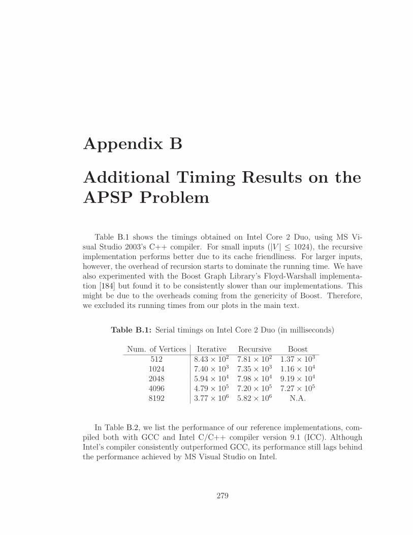
Appendix B
Additional Timing Results on theAPSP Problem
Table B.1 shows the timings obtained on Intel Core 2 Duo, using MS Vi-sual Studio 2003’s C++ compiler. For small inputs (|V | ≤ 1024), the recursiveimplementation performs better due to its cache friendliness. For larger inputs,however, the overhead of recursion starts to dominate the running time. We havealso experimented with the Boost Graph Library’s Floyd-Warshall implementa-tion [184] but found it to be consistently slower than our implementations. Thismight be due to the overheads coming from the genericity of Boost. Therefore,we excluded its running times from our plots in the main text.
Table B.1: Serial timings on Intel Core 2 Duo (in milliseconds)
Num. of Vertices Iterative Recursive Boost512 8.43× 10² 7.81× 10² 1.37× 10³
1024 7.40× 10³ 7.35× 10³ 1.16× 10⁴
2048 5.94× 10⁴ 7.98× 10⁴ 9.19× 10⁴
4096 4.79× 10⁵ 7.20× 10⁵ 7.27× 10⁵
8192 3.77× 10⁶ 5.82× 10⁶ N.A.
In Table B.2, we list the performance of our reference implementations, com-piled both with GCC and Intel C/C++ compiler version 9.1 (ICC). AlthoughIntel’s compiler consistently outperformed GCC, its performance still lags behindthe performance achieved by MS Visual Studio on Intel.
279
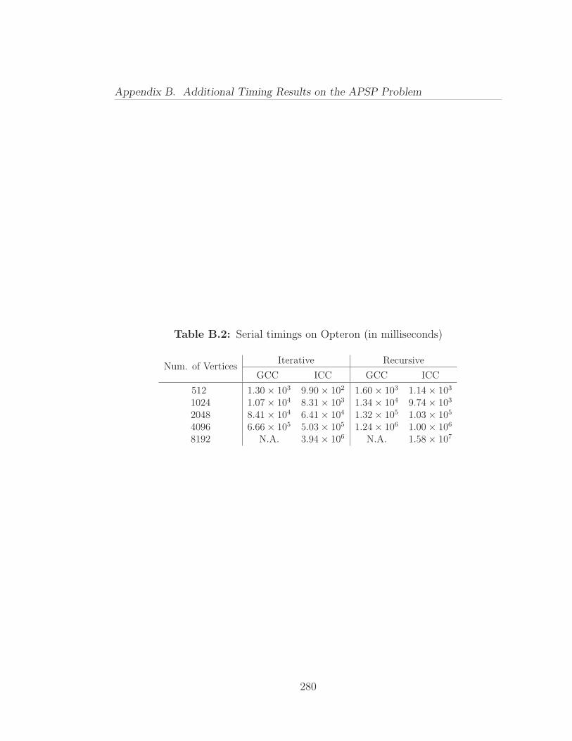
Appendix B. Additional Timing Results on the APSP Problem
Table B.2: Serial timings on Opteron (in milliseconds)
Num. of VerticesIterative Recursive
GCC ICC GCC ICC
512 1.30× 10³ 9.90× 10² 1.60× 10³ 1.14× 10³
1024 1.07× 10⁴ 8.31× 10³ 1.34× 10⁴ 9.74× 10³
2048 8.41× 10⁴ 6.41× 10⁴ 1.32× 10⁵ 1.03× 10⁵
4096 6.66× 10⁵ 5.03× 10⁵ 1.24× 10⁶ 1.00× 10⁶
8192 N.A. 3.94× 10⁶ N.A. 1.58× 10⁷
280


![On Cayley graphs of algebraic structures - arXiv · 2018-03-26 · arXiv:1803.08518v1 [cs.DM] 22 Mar 2018 On Cayley graphs of algebraic structures Didier Caucal1 1 CNRS, LIGM, France](https://static.fdocuments.in/doc/165x107/5f372d6c360c9e616b3802fb/on-cayley-graphs-of-algebraic-structures-arxiv-2018-03-26-arxiv180308518v1.jpg)