Phil Curnock ADS SC21 Manager. What is the SC21 process Model.

Linear Algebra II - Dr AG Curnock
Large Lecture Course
I gave this set of Lectures at the Mathematical Institute, University of Oxford, HT
2007- 2009.
My thanks go to the students who attended and gave feedback
1

Contents
1 Review 4
1.1 Recap of Vector Spaces and Rn . . . . . . . . . . . . . . . . . . . . . 4
1.2 Linear Transformations and Representing Matrices . . . . . . . . . . 5
2 Permutations 12
3 Parity 19
4 Determinants 21
4.1 Determinants for n× n Matrices . . . . . . . . . . . . . . . . . . . . . 24
4.2 Determinants using the Method of row reduction to
echelon form : Consequences of theorem 4.12 . . . . . . . . . . . . . . 28
5 Uniqueness of Determinants 31
6 Final Properties of Determinants 32
7 Applications of Determinants :
Cross Products and Triple Scalar Products 35
7.1 Triple Scalar Product . . . . . . . . . . . . . . . . . . . . . . . . . . . 36
8 Determinants and Linear Transformation 37
9 Polynomials of linear Transformations and Matrices 38
10 Eigenvalues and Eigenvectors 40
10.1 Motivation . . . . . . . . . . . . . . . . . . . . . . . . . . . . . . . . . 40
11 The Characteristic Polynomial 44
12 Diagonalisation of Linear Transformations 47
13 Diagonalisation of Matrices 49
14 Applications of Eigenvectors to linear systems of first order Ordinary
Differential Equations 53
2

Outline
Eight lectures to First year -Mods Students
Review of a matrix of a linear transformation with respect to bases, and change
of bases.
Permutations and related topics. Determinants of square matrices; properties of
the determinant function; determinants and the scalar triple product.
Methods for Computation of determinant. Proof that a square matrix is invertible
if and only if its determinant is non-zero. Determinant of a linear transformation of
a vector space to itself.
Eigenvalues of linear transformations of a vector space to itself. The characteristic
polynomial of a square matrix and its uses. The linear independence of a set of
eigenvectors associated with distinct eigenvalues; diagonalisation of matrices.
Recommended Bibliography
1. C. W. Curtis, Linear Algebra - An Introductory Approach, Springer (4th edi-
tion), reprinted 1994
2. R. B. J. T. Allenby, Linear Algebra, Arnold, 1995
3. T. S. Blyth and E. F. Robertson, Basic Linear Algebra, Springer, 1998
4. I. N. Herstein Topics in Algebra 1977, Wiley International Editions
5. P.G. Kumpel and J.A. Thorpe Linear Algebra
6. S. Lang Linear Algebra, Springer Undergraduate Mathematics Series, 1999
7. B. Seymour Lipschutz, Marc Lipson, Linear Algebra, Third Edition 2001
8. D. A. Towers, A Guide to Linear Algebra, Macmillan, 1988
For Permutations :
9. R.B.J.T. Allenby Rings, Fields and Groups, Second Edition, Edward Arnold,
1999.
10. D.A. Wallace Groups, Rings, and Fields. Springer Undergraduate Mathematics
Series,
3

Lecture 1
1 Review
1.1 Recap of Vector Spaces and Rn
So far you will have looked at the vector space structure of Rn, properties such as :
• zero vector;
• addition of vectors;
• scalar multiplication of vectors (by elements in R/C, or more generally in a
Field);
• multiplication by negative scalars and we also have subtraction of vectors;
• we have a basis - n vectors which span the vectors space and which are linearly
independent.
Rn is a prototype for any vector space. In fact it’s much more - it’s the prototype
for many algebraic, geometric and topological structures. We will look at some of
these over this course of lectures.
Bases
Spanning set- generates the space and so every element of the vector space can be
written as a linear combination of vectors from the basis. The basis is a maximal set -
if we increase it - it’s no longer linearly independent. The basis vectors don’t have to
be mutually perpendicular - but there is such a canonical basis in Rn, and we denote
these by {e1, e2, ..., en} where ei have zero entries everywhere except at the ith entry
it has a 1.
Bases are used in vector spaces to provide a method of computation. Two notions
related to this are how to express (uniquely) a vector in terms of a given basis (studied
in the MT course ) and how to relate co-ordinate systems if you have two different
bases on the same vector space.
Suppose we have a basis B = {v1, ..., vn} of a vector space V . This means that
every v ∈ V can be expressed as a linear combination of elements of the basis:–
4

v = λ1v1 + λ2v2 + ...+ λnvn
where λi ∈ F . (Such a representation is unique as vi are linearly independent) and
so λi are completely determined by v and B. For this reason we may call the scalars
λ1 ..., λn called the co-ordinates of v wrt. basis {v1, ..., vn} and
λ1...
λn
is called
the co-ordinate vector for v wrt this basis.
This tells us something important : to each v ∈ V ←→ n-tuple (λ1, ..., λn) ∈ F n.
Conversely if (λ1, ..., λn) is an n-tuple in F n then ∃ a vector in V of the form
λ1v1 +λ2v2 + ...+λnvn. This tell us there is a 1− 1 correspondence between elements
of V and elements of F n, which gives us a theorem :
Theorem 1.1. If V is a finite dimensional vector space over a field F , then V and
F n are isomorphic (they are identical except possibly with different labels).
1.2 Linear Transformations and Representing Matrices
This section is largely based on D.A. Towers or A.O. Morris (see the bibliography
for details). Let V and W we finite-dimensional vector spaces over a field F and
T : V → W be a linear transformation. Consider bases BV = {v1, v2, . . . , vn} and
BW = {w1, w2, . . . , wm} for V and W respectively.
We may express the image of each vi under T as a linear combination of elements
of BW , namely
T (v1) = a11w1 + . . . + am1wm...
......
......
...
T (vi) = a1iw1 + . . . + amiwm...
......
......
...
T (vn) = a1nw1 + . . . + amnwm
(1.1)
collecting the coefficients (we choose to do this in columns - the so-called column
convention) gives us a matrix
A = (aij), called the Matrix Representation of T ,
5

or the Transition matrix of T . Here the aij belong to F. Note that A is the
transpose of the matrix given in set of equations in (1.1). Thus
T (vi) =∑j=1,m
ajiwj for each i
As BW is a basis, the coefficients in the equations (1.1) are uniquely determined. If
we wish to emphasise the bases used to find A we write MBVBW (T ) for A.
Example 1.2. Let T : R3 → R2 given by T ((x, y, z)t) = (2x+ y, y + z)t.
Take the standard bases for R3 and R2 denoting them by B1 and B2 respectively.
Write down the matrix for T ; we call this matrix A = MB1B2 (T ).
Solution Firstly T ((1, 0, 0)t) = (2, 0)t = 2(1, 0)t + 0(0, 1)t; T ((0, 1, 0)t) = (1, 1)t =
1(1, 0)t + 1(0, 1)t and
T ((0, 0, 1)t) = (0, 1)t = 0(1, 0)t + 1(0, 1)t which gives us A =
(2 1 0
0 1 1
).
Example 1.3. Let V be an n-dimensional vector space over a field R and id : V → V
be the identity transformation. Then for any basis B on V the matrix MBB (id) = In.
Remark We may write idV but for ease of notation, often write id except when we
wish to emphasise the domain.
CAUTION : If we work with distinct bases B1,B2 on V then MB1B2 (id) 6= In, but we
will shortly have a result relating these two matrices (Corollary 1.6 below). Firstly
we see how to compute MB1B2 (id) applying T = id to the equations in (1.1).
Example 1.4. Let V = R3 and consider the identity mapping id : R3 → R3.
Find MB1B2 (id) when B1 = {(1, 5, 0)t, (−1, 0, 2)t, (0, 4, 1)t} and
B2 = {(−2, 1, 2)t, (2, 3,−1)t, (−1,−1, 1)t} are bases for V.
Solution We will find coefficients a11, a21, a31 which are found by solving
1
5
0
= a11
−2
1
2
+ a21
2
3
−1
+ a31
−1
−1
1
6

These give us a11 = 1, a21 = 1 and a31 = −1.
Continuing in this way gives us the matrix
MB1B2 (id) =
1 0 1
1 1 1
−1 3 0
.
In fact we draw together results from your MT course relating simple properties
of matrices of the form MBVBW (T ) into one Proposition.
Proposition 1.5. Let S and T be linear transformations and V and W vector spaces
over a field F. Suppose S : V → W and T : V → W where V and W have bases BVand BW respectively. Then the following hold
(i) MBVBW (S + T ) = MBV
BW (S) +MBVBW (T );
(ii) MBVBW (λT ) = λMBV
BW (T );
(iii) If R : W → U where U is a vector space over F with basis BU then
MBVBU (R ◦ T ) = MBW
BU (R)×MBVBW (T );
(iv) If T is Invertible then MBWBV (T−1) = MBV
BW (T )−1.
Proof. See your MT Notes.
This immediately gives us the following Corollary:
Corollary 1.6. Let V be an n-dimensional vector space over a field R and B1,B2 be
distinct bases on V. Then
MB1B2 (id)×MB2
B1 (id) = In.
and so MB1B2 (id) is always invertible.
Proof. Apply the result in part (iii) above.
The above Proposition also gives us our first Change of Basis Theorem.
7

Theorem 1.7 (Change of Basis 1). Let V be a finite-dimensional vector space over
a field F (e.g. R) with distinct bases B1 and B2 and T : (V,Bi)→ (V,Bi) be a linear
transformation for i = 1, 2. Then there exists an invertible matrix P such that
MB2B2 (T ) = PMB1
B1 (T )P−1,
and in fact we may take P = MB1B2 (id)
Proof. Simply draw a mapping diagram and construct T as a composition operator
and apply (iii) in Proposition 1.5.
Question :What happens if we have a general linear transformation
We are interested in changing the basis and to see what effect this has on the
matrix form of the linear transformation. We will look at three cases via examples
before stating the results formally. Namely considering :
(i) Changing the basis on the domain;
(ii) Changing the basis on the co-domain;
(iii) Changing the bases on both the domain and co-domain.
Example 1.8. Let T : R3 → R2 given by T ((x, y, z)t) = (2x + y, y + z)t. Refer
to Example 1.2 above where we used standard bases for the domain and co-domain
arriving at a matrix A.
(i) Take a new basis for the domain given by B′1 = {(1, 1, 0)t, (0, 1, 0)t, (1, 1,−1)t}but keep the standard basis for the co-domain. Find the matrix B which rep-
resents T w.r.t. these bases.
State the relationship between A,B and MB′1B1 (id);
(ii) Take a new basis for the co-domain given by B′2 = {(1, 1), (1, 0)} but keep the
standard basis for the domain. Find the matrix C which represents T w.r.t.
these bases.
State the relationship between A,C and MB2B′2
(id);
8

(iii) Take the above new bases for R3 and R2. Find the matrix D which represents
T w.r.t. these bases.
State the relationship between A,D, and MB′1B′2
(id).
Solution Recall A =
(2 1 0
0 1 1
).
(i) Changing the basis on the domain means that T maps the new basis vectors
to T ((1, 1, 0)t) = (3, 1)t = 3(1, 0)t + 1(0, 1)t;T ((0, 1, 0)t) = (1, 1)t = 1(1, 0)t +
1(0, 1)t and
T ((1, 1,−1)t) = (3, 0)t = 3(1, 0)t+0(0, 1)t which gives us B =
(3 1 3
1 1 0
). To
find the relationship between A and B we need to compute MB1B′1
(id). As with
the above example,
(1, 0, 0)t = 1(1, 1, 0)t − 1(0, 1, 0)t + 1(1, 1,−1)t
etc which gives us MB1B′1
(id) =
1 0 1
−1 1 0
0 0 −1
.
We see that if we post-multiply A by MB1B′1
(id)−1 we will have B,
i.e. B =
(2 1 0
0 1 1
)×
1 0 1
1 1 1
0 0 −1
=
(3 1 3
1 1 0
).
Formally
B = New matrix for T = MB′1B2 (T ) = A×MB1
B′1(id)−1.
[To prove this : look at the matrices as mappings w.r.t. the given bases and use
the result that composing mappings is equivalent to multiplying the matrices.
Here we would be assuming Prop 1.5. In the lecture we proved this without
assuming 1.5 but just using first principles.]
(ii) Computing as above, for example T ((1, 0, 0)t) = (2, 0)t = 0(1, 1)t + 2(1, 0)t we
have
C =
(0 1 1
2 0 −1
)
9

and if we pre-multiply A by MB2B′2
(id), we will have the matrix representation
for T w.r.t. the new basis on the co-domain. Thus
C = MB1B′2
(T ) = MB2B′2
(id)× A;
(Hint : Here you will find that MB2B′2
(id) =
(0 1
1 −1
)and it is straightforward
to prove the relationship in (ii).)
(iii) This is the most general form. Again compute T ((1, 1, 0)t) = (3, 1)t = 1(1, 1)t+
2(1, 0)t etc, which gives us
D =
(1 1 0
2 0 3
)
and we should find that
D = MB′1B′2
(T ) = MB2B′2
(id)× A×MB1B′1
(id)−1.
(or MB′1B′2
(T ) = QAP−1.)
Exercise 1.9. Confirm these last two calculations. Further exercises and examples
may be found in, for example, D.A. Towers or A.O. Morris.
We can state this latter result formally as our second Change of Basis Theorem
(which is sometimes called the QAP−1 Theorem.)
Theorem 1.10. (Change of Basis 2) Let V and W be vector spaces over a field F
and suppose V has a basis B1 and W has a basis B2. Let T : (V,B1) → (V,B2) be
a linear transformation w.r.t. these bases. Suppose B′1 and B′2 are new bases for the
domain and co-domain respectively.
Then
MB′1B′2
(T ) = MB2B′2
(idW )× A×MB1B′1
(idV )−1.
Proof. Consider the composition of map T = idW ◦T ◦idV with respect to the following
bases:
10

VidV−−−→ V
T−−→ WidW−−−→ W.
basis B′1 basis B1 basis B2 basis B′2.
Then
MB′1B′2
(T ) = MB′1B′2
(idW ◦ T ◦ idV )
= MB′2B2 (idW ) ◦MB1
B2 (T ) ◦MB′1B1 (idV )
and by Proposition 1.5 and its Corollary, the required form appears. (i.e. by inter-
changing the bases on the final righthand matrix and taking its inverse.)
11

Lecture 2
2 Permutations
We wish to study the Determinant of a linear transformation and to do so we will need
the concept of a Permutation, its sign and some simple properties. Permutations will
be re-visited in the next course on Groups, Rings and Fields; we follow the conventions
of Herstein and Dr W.B.S. Stewart (see booklist).
Let X be the set {x1, x2, . . . , xn} then a permuatation σ of X is a bijection from
X onto itself. Such a mapping may be written as
σ =
(x1 x2 . . . xn
(x1)σ (x2)σ . . . (xn)σ
).
N.B. For functions and linear transformations you are used to writing x → f(x)
or x → T (x) however in abstract algebra the convention is to write (x)f when no
confusion is likely (so if you are reading books : check what convention is used).
The set of all permutations on X is given by SX . We will only consider finite sets
X and so we may as well take X = {1, 2, . . . , n} (as there is always a bijection from
X onto this set) and we write Sn in place of SX , noting that Sn has precisely n!
elements.
We look at some examples to help build the theory of permutations.
Example 2.1. Let σ be a permutation in S3 given by 1 7→ 2, 2 7→ 1 and 3 7→ 3. One
notation for σ is to write the inputs in a row with the outputs in a row below each
input.
σ =
(1 2 3
2 1 3
)We tend to write the top row in increasing order but equally the order in which
we write each column can be changed around and still give the same permutation.
The important thing that matters is that we keep the input with its output. So we
could equally write
σ =
(2 3 1
1 3 2
)=
(3 1 2
3 2 1
).
The images of 1, 2 and 3 are the same in each.
12

Composition and Inverses of Permutations
We have seen that we write (1)σ to denote the image of an element under the per-
mutation σ. We omit the brackets from now on unless we need them for clarity.
Definition 2.2. Let π, σ ∈ Sn. If π =
(1 2 . . . n
1π 2π . . . nπ
), and σ =
(1 2 . . . n
1σ 2σ . . . nσ
),
then the composition π ◦ σ which means do π followed by σ, is denoted by
π ◦ σ =
(1 2 . . . n
(1π)σ (2π)σ . . . (nπ)σ
).
By the Identity mapping we mean the mapping ι which sends each element to
itself.
If π is defined as above, then the inverse π−1 is found by reading the columns
upwards, i.e. 1π 7→ 1, 2π 7→ 2 etc, giving us π−1 =
(1π 2π . . . nπ
1 2 . . . n
)and
π ◦ π−1 = ι.
We would normally re-arrange the columns of π−1 so that elements in the top row
are in increasing order (keeping the input with its output).
Example 2.3. If π =
(1 2 3
2 1 3
)and σ =
(1 2 3
2 3 1
),
find π ◦ σ, σ ◦ π, and π−1, σ−1. Check that π ◦ π−1 = ι. What is (π ◦ σ)−1 in terms
of π and σ?
Solution π ◦ σ =
(1 2 3
2 1 3
)◦
(1 2 3
2 3 1
). Starting from the left, 1 7→ 2 in π
and 2 7→ 3 in σ, so 1 7→ 3. So we have
π ◦ σ =
(1 2 3
3 2 1
). Similarly σ ◦ π =
(1 2 3
1 3 2
).
As we would expect, permutations do not generally commute under composition.
π−1 =
(2 1 3
1 2 3
)=
(1 2 3
2 1 3
).
[Check : π−1 ◦ π =
(1 2 3
2 1 3
)◦
(1 2 3
2 1 3
)=
(1 2 3
1 2 3
).]
13
Exercise 2.4. Complete this example, in particular, see that (π ◦ σ)−1 = σ−1 ◦ π−1.Prove this for permutations in Sn.
This two-row notation is limited : it does not help us to see the structure of the
permutation, so we now look at cycle notation and cycle structure.
Structure of Permutations : Orbits and Cycles
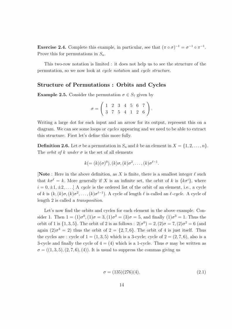
Example 2.5. Consider the permutation σ ∈ S7 given by
σ =
(1 2 3 4 5 6 7
3 7 5 4 1 2 6
).
Writing a large dot for each input and an arrow for its output, represent this on a
diagram. We can see some loops or cycles appearing and we need to be able to extract
this structure. First let’s define this more fully.
Definition 2.6. Let σ be a permutation in Sn and k be an element inX = {1, 2, . . . , n}.The orbit of k under σ is the set of all elements
k(= (k)(σ)0), (k)σ, (k)σ2, . . . , (k)σ`−1.
[Note : Here in the above definition, as X is finite, there is a smallest integer ` such
that kσ` = k. More generally if X is an infinite set, the orbit of k is {kσi}, where
i = 0,±1,±2, . . . .] A cycle is the ordered list of the orbit of an element, i.e., a cycle
of k is (k, (k)σ, (k)σ2, . . . , (k)σ`−1). A cycle of length ` is called an `-cycle. A cycle of
length 2 is called a transposition.
Let’s now find the orbits and cycles for each element in the above example. Con-
sider 1. Then 1 = (1)σ0, (1)σ = 3, (1)σ2 = (3)σ = 5, and finally (1)σ3 = 1. Thus the
orbit of 1 is {1, 3, 5}. The orbit of 2 is as follows : 2(σ0) = 2, (2)σ = 7, (2)σ2 = 6 (and
again (2)σ3 = 2) thus the orbit of 2 = {2, 7, 6}. The orbit of 4 is just itself. Thus
the cycles are : cycle of 1 = (1, 3, 5) which is a 3-cycle; cycle of 2 = (2, 7, 6), also is a
3-cycle and finally the cycle of 4 = (4) which is a 1-cycle. Thus σ may be written as
σ = ((1, 3, 5), (2, 7, 6), (4)). It is usual to suppress the commas giving us
σ = (135)(276)(4). (2.1)
14

We saw in our diagram (and in the above notation) that these cycles were disjoint
- here we have a permutation which is written as a “Product of Disjoint Cycles.”
This is a property we can prove more generally.
[Caution : removing commas as in 2.1 might lead to ambiguity. For example, how
do we distinguish between (1, 2, 3) and (1, 23)? We avoid confusion by pre-fixing a
blank space in front of each numeral in a cycle. Thus writing the above as ( 1 2 3)
and ( 1 23). ]
Our next example gives permutations which are one `-cycles.
Example 2.7. (i) Let σ =
(1 2 3 4 5 6
2 4 5 6 1 3
).
We can see that 1 7→ 2 7→ 4 7→ 6 7→ 3, 3 7→ 5 and 5 7→ 1. It is now clear that
when looking for cycles, the first row of the permutation is somewhat redundant.
What needs to be recorded is this chain order and so we adopt the following
cycle notation : Thus σ = ( 1 2 4 6 3 5) and σ is a 6-cycle.
(ii) Let π =
(1 2 3 4 5 6
5 2 1 4 3 6
). Notice that elements 2, 4 and 6 are fixed under
π and so these are not listed in the cycle notation. The cycle flows from the
following map : 1 7→ 5, 5 7→ 3, 3 7→ 1 and all the elements have been used. Thus
π = ( 1 5 3), a 3-cycle.
(iii) List all the permutations in S3 and express each as a cycle. (Our convention
will be to omit the 1-cycles).
(1 2 3
1 2 3
), the identity ι, by convention we write ( 1), a 1-cycle,(
1 2 3
2 1 3
)= (12),
(1 2 3
1 3 2
)= (23), and
(1 2 3
3 2 1
)= (13) these
are transpositions - meaning two elements move and the rest are fixed. Also(1 2 3
2 3 1
)= (123),
(1 2 3
3 1 2
)= (132), both are 3-cycles.
This last example gives us motivation for another definition of a cycle :
15
Definition 2.8. A permutations σ ∈ Sn is a cycle of length ` where 2 ≤ ` ≤ n, if
there exist distinct integers ai ∈ {1, 2, . . . , n} for i = 1, 2, . . . ` such that
ai+1 = aiσ for i = 1, 2, . . . , `− 1
a1 = a`σ
b = bσ for b 6= ai, for all i = 1, 2, . . . , `.
Two questions spring to mind : (i) is the representation in 2.1 unique and (ii) are
there other representations? We will come to these shortly. Firstly we need some
more properties.
Remark 2.9. Authors usually omit the 1-cycles although you will need to know they
could be there.
An `-cycle can be written in ` ways (one for each choice of initial element).
Finally some authors use a canonical representation in which the leading number in
a cycle σ is the smallest in the cycle and in which the leading elements increase as we
go through the cycle.
We have the following Theorem which we will state (you must wait for the next
course for its proof!)
Theorem 2.10. Every permutation σ ∈ Sn can be written as a product of disjoint
cycles.
This cycle decomposition is unique up to the order in which the cycles are written
(noting that disjoint cycles commute which needs proving) and up to the choice of
starting element for each cycle.
We now look at 2-cycles, transpositions.
Example 2.11. We first see that permutations (eg cycles) can be written as a product
of transpositions.
(i) Consider ( 1 3 4) ∈ S4 where ( 1 3 4) = ( 1 3)( 1 4). Multiply the RHS we see
that working from left to right
1 7→ 3 1 7→ 4 so in the end 1 7→ 3
2 7→ 2 2 7→ 2 2 7→ 2
3 7→ 1 3 7→ 3 3 7→ 4
4 7→ 4 4 7→ 1 4 7→ 1.
16

It is clear that this is the LHS. Notice that 2 is fixed under all transpositions
on the RHS and on the LHS so we don’t need to consider this element. After a
time you just do all this in your head.
(ii) Show that ( 1 2 3) = ( 1 3)( 2 3) ∈ S4. (Now we can see that this representation
is not unique.)
Then on the RHS we will have
1 7→ 3 1 7→ 1 so in the end 1 7→ 2
2 7→ 2 2 7→ 3 2 7→ 3
3 7→ 1 3 7→ 2 3 7→ 1
(iii) ( 3 6 2 8 5) = ( 3 6)( 2 3)( 3 8)( 5 3) ∈ S8. We can see that on both sides 1,4
and 7 are fixed so we omit these. On the RHS we have
2 7→ 2 2 7→ 3 2 7→ 2 2 7→ 2
3 7→ 6 3 7→ 2 3 7→ 8 3 7→ 5
5 7→ 5 5 7→ 5 5 7→ 5 5 7→ 3
6 7→ 3 6 7→ 6 6 7→ 6 6 7→ 6
8 7→ 8 8 7→ 8 8 7→ 3 8 7→ 8.
Passing through from left to right gives us the LHS.
Exercise : Find a product of transpositions for ( 3 7 5)( 4 6 8).
Generally an `-cycle ( a1 a2 . . . a`) can be written as
( a1 a2 . . . a`) = ( a1 a2)( a1 a3) . . . ( a1 a`)
We will prove this below.
Proposition 2.12. For n ≥ 2, every cycle σ ∈ Sn can be written as a product of
transpositions.
We will complete the proof when next we meet but I add this for you to read.
Proof. By theorem 2.10, it suffices to prove this for σ an `−cycle. Take σ = ( a1 a2 . . . a`)
with ai ∈ {1, 2, . . . , n}. If ` = 1 then for example, σ = (a1) = ( a1, a2) = ι =
( a1, a2)( a2, a1). If ` ≥ 2 then we claim that
( a1 a2 . . . a`) = ( a1 a2)( a1 a3) . . . ( a1 a`)
17

Taking the RHS we can see that a2 is fixed in all the transpositions except the first.
In the first one, a1 maps to a2 which agrees with the LHS. Similarly for each i on the
right, ai is fixed everywhere except in ( a1 ai) when a1 7→ ai. On the left, there is a
connected path from a1 to ai.
This representation is not unique but what is unique is whether there are an odd
or even number of transpositions in a product.
Definition 2.13. We define the Parity of a permutation σ ∈ Sn to be even if we can
express σ in an even number of transpositions; it is odd if we can express σ in an odd
number of transpositions.
18

Lecture 3
3 Parity
We begin with a more formal definition of Parity, in terms of the sign function (or
signature function).
Let p(x1, x2, . . . , xn) be a polynomial and σ be a permutation in Sn. We can
always form a new polynomial in terms of p and σ, namely, pσ(x1, x2, . . . , xn) :=
p(x(1)σ, x(2)σ, . . . , x(n)σ).
Now let P be the polynomial P (x1, x2, . . . , xn) =∏
1≤i<j≤n(xi − xj), then :
Definition 3.1. If σ ∈ Sn then the sign, sign(σ) of σ is defined to be
sign(σ) :=Pσ(x1, x2, . . . , xn)
P (x1, x2, . . . , xn)=P (x(1)σ, x(2)σ, . . . , x(n)σ)
P (x1, x2, . . . , xn).
Equally
sign(σ) =
∏1≤i<j≤n(x(i)σ − x(j)σ)∏
1≤i≤j≤n(xi − xj).
To see how this definition gives us just a ±1 we look at an example.
Example 3.2. Let σ = ( 1 2 3). Compute the sign of σ and check that this agrees
with its parity. Well,
sign(σ) =(x(1)σ − x(2)σ)(x(1)σ − x(3)σ)(x(2)σ − x(3)σ)
(x1 − x2)(x1 − x3)(x2 − x3).
On the numerator we have (x2 − x3)(x2 − x1)(x3 − x1), and so
sign(σ) =(x2 − x3)×−1(x1 − x2)×−1(x1 − x3)
(x1 − x2)(x1 − x3)(x2 − x3)= 1.
Now ( 1 2 3) = ( 1 2)( 1 3) in terms of transpositions, and σ is even and its parity
is +1.
We shall see that for any permutation, the parity of σ coincides with its sign where
sign(σ) = ±1. This needs proving.
19

Lemma 3.3. Let σ ∈ Sn, then the parity of σ is given by its sign. That is, sign(σ) =
+1 if σ is even, and sign(σ) = −1 if σ is odd.
Proof. There are two things to show : (a) that if σ is a transposition, then its sign
is -1; (b)sign is a multiplicative function, namely, if σ, π are permutations in Sn then
sign(σπ) = sign(σ)sign(π).
We begin with (a) : Let σ = ( k `) be a transposition in Sn with k < ` where
h, ` ∈ {1, 2, . . . , n}.By definition we need only consider the factors (x(i)σ−x(j)σ) for any 1 ≤ i ≤ j ≤ n.
We claim that sign( k `) = −1 for k < `. We decompose∏
1≤i≤j≤n(x(i)σ − x(j)σ)
into 4 disjoint sets of indices :
∏1≤i≤j≤n
(x(i)σ − x(j)σ) = (x` − xk)×
×∏
i<j,i6=k,j 6=`
(xi − xj)
×∏
k<j<`,j 6=`
(x` − xj)
×∏
k<i<`,i6=k
(xi − xk).
Looking at the number of sign changes on the RHS we arrive at :
(−1)× (−1)#{j:k<j<`}× (−1)#{i:k<i<`}∏
i<j(xi−xj) which is −1∏
i<j(xi−xj) and
so the sign of a transposition is -1.
(b) Finally let σ, π be permutations in Sn.
Then
sign(σπ) =Pσπ(x1, x2, . . . , xn)
P (x1, x2, . . . , xn)
=P (x(1)σπ, x(2)σπ, . . . , x(n)σπ)
P (x1, x2, . . . , xn)
=P (x(1)σ, x(2)σ, . . . , x(n)σ) · P (x(1)σπ, x(2)σπ, . . . , x(n)σπ)
P (x1, x2, . . . , xn) · P (x(1)σ, x(2)σ, . . . , x(n)σ).
Letting yi = (xi)σ in the numerator and denominator on the right we have
sign(σπ) = sign(σ)(π)
20

To conclude the proof we note that if σ1, σ2, . . . , σk are transpositions and σ =
σ1σ2 . . . σk then
sign(σ) = sign(σ1σ2 . . . σk) = sign(σ1) sign(σ2) . . . sign(σk) = (−1)k.
Hence if k is the number of transpositions in σ then if k is odd, sign(σ) = −1 and if
k is even, sign(σ) = +1.
We have now built sufficient machinery to be able to proof results about Deter-
minants.
4 Determinants
Much of this section is based on Hersteins’ Topics in Algebra, and Curtis’ Linear
Algebra.
A determinant is a scalar we associate with a square matrix, formally if A is a
matrix in Mn×n(F ) where F is a field of scalars (eg R), then the determinant of
A,det(A) (or |A|) is det(A) : F n → F. Determinants play a key role in the solution
of a system of linear equations. (We shall see that det(A) 6= 0 ⇔ A is non-singular
- it has an inverse). Determinants also give us some useful geometrical information
about the transformation that the matrix represents.
Geometric Motivation for Determinants
We shall see that geometrically the determinant is the volume of a parallelepiped
whose edges are the rows of the matrix (up to a ± sign).
Consider a parallelogram in the plane whose edges are the vectors {a1, a2}. Con-
sider a function that computes the area A(a1, a2) of such a parallelogram. What
properties would be desirable?
We would hope this area function A has the following properties :
A1 A(e1, e2) = 1 where ei are the usual basis vectors of R2;
A2 A(λa1, a2) = A(a1, λa2) = λA(a1, a2) for any ai ∈ R2, and λ ∈ R;
A3 A(a1 + a2, a2) = A(a1, a2) = A(a1, a1 + a2) for any ai ∈ R2,.
21

We shall prove that these properties characterise a Determinant Function and
moreover we have a useful test for the independence of two vectors from the above
properties A1 - A3:
A(a1, a2) 6= 0 iff {a1, a2} are linearly independent.
Computation of 2× 2 and 3× 3 matrices
This will be familiar to you.
Definition 4.1. 1. If A = (a) then its determinant, det(A) = a
2. If A =
(a b
c d
)then det(A) = |A| =
∣∣∣∣∣ a b
c d
∣∣∣∣∣ = ad− bc.
So for a diagonal matrix, A =
(a 0
0 d
)then det(A) = ad which is the product
of its diagonal elements . Notice that if we switch a column in A then the sign of the
determinant changes. (i.e. |A′| =
∣∣∣∣∣ b a
d c
∣∣∣∣∣ = bc− ad = −|A|.
We can make some further simple observations.
1. If we form the matrix A′ by adding row 2 to row 1, r1 → r1 + r2, we leave the
determinant unchanged.
i.e. det(A′) =
∣∣∣∣∣ a+ c b+ d
c d
∣∣∣∣∣ = (a+ c)d− (b+ d)c = ad− bc = |A|.
2. If we form the matrix A′′ by multiply a row by a scalar, say r1 → λr1, the
determinant changes by this factor. i.e.
i.e. det(A′′) =
∣∣∣∣∣ λa λb
c d
∣∣∣∣∣ = λad− λbc = λ(ad− bc) = λ|A|.
Method of Cofactors
Definition 4.2. Let A be a 3× 3 matrix where A =
a11 a12 a13
a21 a22 a23
a31 a32 a33
.
We define the Minor of an element aij to be the 2 × 2 determinant formed by
deleting the row and column from A in which aij occurs.
22

For example, the
Minor of a23 =
∣∣∣∣∣ a11 a12
a31 a32
∣∣∣∣∣ = a11a32 − a12a31.
Superimposing a chequerboard pattern of signs on A, namely
+ − +
− + −+ − +
,
we define the Cofactor of aij to be the signed minor, denoted by Aij. For example,
A23 = −(a11a32 − a12a31).
Definition 4.3. If A is a 3× 3 matrix, we define its determinant to be
|A| =
j=3∑j=1
aijAij and i = 1, 2 or 3 (4.1)
=i=3∑i=1
aijAij and j = 1, 2 or 3. (4.2)
The two equations in 4.1 and 4.2 are known as the Laplace expansions of the
determinant of A by the i-th row and j-th column, respectively.
Example 4.4. Expand A by r1 using the above 4.1.
Solution |A| = a11(a22a33−a23a32)−a12(a21a33−a23a31)+a13(a21a32−a22a31) which
gives is |A| in terms of 6 products, each of three elements with exactly one from each
row and column.
|A| = a11a22a33 − a11a23a32 − a12a21a33 + a12a23a31 + a13a21a32 − a13a22a31.Note : a) The subscripts are all of the form 1, (1)σ 2, (2)σ 3, (3)σ. (For clarity we
use a comma between the first subscript and its image under σ.)
b) The second product has the sign −1 as this is an odd permutation. Here 1 7→1, 2 7→ 3, 3 7→ 2 so as cycles is ( 1)( 2 3) and as a product of (one) transposition is
( 2 3).
c) Similarly in the fourth product its subscripts send 1 7→ 2, 2 7→ 3, 3 7→ 1, which is
the cycle ( 1 2 3) = ( 1 2)( 1 3) which is even.
Example 4.5. Evaluate |A| where A =
2 3 1
5 0 −1
7 2 4
. If we interchange the first
and second column, what happens to the determinant?
23

Solution Expanding by the first row gives us
|A| =j=3∑j=1
a1jA1j = +2
∣∣∣∣∣ 0 −1
2 4
∣∣∣∣∣− 3
∣∣∣∣∣ 5 −1
7 4
∣∣∣∣∣+ 1
∣∣∣∣∣ 5 0
7 2
∣∣∣∣∣ = −67.
We should notice a change in sign if we swop two columns.
Exercise 4.6. State what happens to the value of the determinant if (i) a row or
column in the above 3 × 3 matrix ia zero? (ii) we multiply a row or column by a
scalar, eg, λ, (iii) if we add a multiple of λ row 1 to row 3?
It is clear that for larger matrices we need some theory to help us find more
efficient expansions of a determinant.
Lecture 4
4.1 Determinants for n× n Matrices
We now give a formal definition of a determinant. Recall that we saw in the case of
a 2 × 2 matrix that the interchange of two columns produced a sign change in the
determinant. This is precisely the sign or parity of a permutation on the number of
transpositions of the subscripts (regarded as cycles).
Let A be a matrix in Mn(R). We define the determinant of A to be the algebraic
sum of all products of n elements from A which is formed by selecting exactly one
element from each row and column of A.
Definition 4.7 (Determinant of Matrix). If a matrix A = (aij) and A ∈Mn(R) then
the determinant of A is given by
det(A) :=∑σ∈Sn
sign(σ) a1,(1)σ a2,(2)σ . . . an,(n)σ,
where the sum is over all permutations σ ∈ Sn. Equally
det(A) :=∑σ∈Sn
(−1)σ a1,(1)σ a2,(2)σ . . . an,(n)σ,
where (−1)σ denotes the parity of σ which is +1 if the permutation σ is even, and
−1 is σ is odd.
24

It is not difficult to see that this agrees with our earlier definition of a determinant
for small matrices in terms of cofactors but also generalises the method of cofactors to
n×n matrices. However given n! products in each determinant such a definition does
not readily help us compute determinants. The definition tells us that the determinant
of a matrix will be zero if any row or column is zero.
We now establish some natural properties of the determinant, regarded as a func-
tion of the rows of a matrix. For this let A ∈ Mn(R) where the ith row of A is ri,
then it is natural to write :
Det(A) := D(r1, . . . , ri, . . . , rn).
A natural question is what properties does D have? We shall see that it satisfies
the Elementary Row Operations and so this will enable us to prove that we can row
reduce a matrix to echelon form to determine its determinant.
Theorem 4.8. The function D on a matrix in Mn(R) is linear in rows, that is,
D1 D(r1, . . . , ri, . . . , rn) +D(r1, . . . , r′i, . . . , rn) = D(r1, . . . , ri + r′i, . . . , rn) ∀i;
D2 D(r1, . . . , ri−1, λri, ri+1, . . . , rn) = λD(r1, . . . , ri, . . . , rn), for all λ ∈ R, λ 6= 0, ∀i ;
Also
D3 D(e1, e2, . . . , en) = 1, for ei the usual ith unit vector in Rn.
Proof. D1 On the right we have
∑σ
(−1)σ a1,(1)σ . . . (ai,(i)σ + a′i,(i)σ) . . . a1(1)σ . . . an,(n)σ
and as only the ith row is changed, and summation is additive, we have :∑σ∈Sn
(−1)σ a1,(1)σ . . . ai(i)σ . . . . . . an,(n)σ +∑σ
(−1)σ a1(1)σ . . . a′i,(i)σ . . . . . . an,(n)σ.
25

D2 Again only entries in the i-th row change. On the left we have
∑σ∈Sn
σ(−1)σa1,(1)σ . . . ai−1,(i−1)σ λai,(i)σ ai+1,(i+1)σ . . . an,(n)σ =
λ∑σ∈Sn
(−1)σ a1,(1)σ . . . ai,(i)σ . . . an,(n)σ,
as summation is linear.
D3 D(e1, e2, . . . , en) =∑
σ(−1)σe1,(1)σ . . . ei,(i)σ . . . en,(n)σ where ei,(j)σ = 1 if
i = j, and zero otherwise. Hence the result follows.
Note that D3 tells us that D(In) = 1, or that D is 1− preserving.
Proposition 4.9. If we interchange two rows the resulting determinant is changed
by a factor of −1, that is,
D(r1, . . . , ri, . . . , rj, . . . , rn) = −D(r1, . . . , rj, . . . , ri, . . . , rn)
for all i, j ∈ {1, 2, . . . , n}, i 6= j; D is called Alternating.
Proof. If A is the original matrix, then
|A| =∑σ∈Sn
sign(σ) a1,(1)σa2,(2)σ . . . ai,(i)σ . . . aj(j)σ . . . an,(n)σ.
But if A′ is the matrix A with the ith and jth row interchanged, then
|A′| =∑σ∈Sn
sign(σ) a1,(1)σa2,(2)σ . . . aj,(j)σ . . . ai,(i)σ . . . an,(n)σ.
If we think of the sign(σ) in terms of the definition of the polynomials given in 3.1
we will see that ( (1)σ (2)σ . . . (j)σ . . . (i)σ . . . (n)σ) = −1( (1)σ 2(σ) . . . (i)σ . . . (j)σ . . . (n)σ)
applying Lemma 3.3) as it is a transposition. Thus |A′| = −|A|.
We shall call a function which satisfies D1, D2, and D3 and is Alternating a
Determinant function.
26

Proposition 4.10. If we replace row ri in a determinant by row ri + λrj the deter-
minant is unchanged, namely,
D(r1, . . . , ri, . . . , rn) = D(r1, . . . , (ri + λrj), . . . , rn),
for all λ ∈ R, and for all i, j, i 6= j, 1 ≤ i, j ≤ n.
[This will be set as an Exercise in the lecture.]
Proof.
D(r1, r2, . . . , ri, . . . , rj . . . , rn)
=1
λD(r1, r2, . . . , ri, . . . , λrj . . . , rn) by D2,with λ 6= 0
=1
λD(r1, r2, . . . , ri + λrj, . . . , λrj . . . , rn) byD1′
=λ
λD(r1, r2, . . . , ri + λrj, . . . , rj . . . , rn) by D2.
[To be precise D1′ is a modified form of D1, where
D1′ : D(r1, . . . , ri, . . . , rn) +D(r1, . . . , ri, . . . , rj, . . . rn) = D(r1, . . . , ri + rj, . . . , rn)
for all i 6= j.
which may be proved in a similar manner to D1.
Remark 4.11. Theorem 4.8 and Proposition 4.9 tell us that the Determinant Func-
tion D has all the geometric properties that the Area Function had, and in fact they
tell us something more important. The Properties D1, D2, D3 and Alternating com-
pletely characterise the Determinant function : given another function that satisfies
the properties D1, D2, D3 and is alternating then this agrees with the definition of
the determinant,
Det(A) =∑σ∈Sn
sign(σ) a1(1)σ a2(2)σ . . . an(n)σ.
(We shall prove this in the next lecture.)
Theorem 4.12. Let D be the determinant function of a matrix A ∈ Mn(R) let A
have rows {r1, r2, . . . , rn} then the following statements hold :
27

(a) If A′ is the matrix obtained from A by interchanging two rows (ri and rj are
interchanged where i 6= j), then
|A′| = −|A|.
This amounts to performing an elementary row operation of type I;
(b) If A′ is the matrix obtained from A by replacing ri by λri for any i with λ ∈ R,then
|A′| = λ|A|.
This amounts to performing an elementary row operation of type II;
(c) If A′ is the matrix obtained from A by replacing ri by ri + λrj for any row
rj, j 6= i and λ ∈ R, then
|A′| = |A|.
This amounts to performing an elementary row operation of type III;
(d) D(r1, r2, . . . , rn) = 0 if any two rows are equal;
(e) D(r1, r2, . . . , rn) = 0 if {r1, r2, . . . , rn} is linearly dependent.
Proof. Parts (a),(b) and (c) follow immediately from Theorem 4.8, and Propositions
4.9 and 4.10. Case (d) holds since if we subtract the two identical rows then one
element of each product of the determinant is zero. Case (e) holds by applying part
(c) then (d).
4.2 Determinants using the Method of row reduction to
echelon form : Consequences of theorem 4.12
Let A ∈ Mn(R). Theorem 4.12 gives us a method for evaluating a determinant by
applying Elementary Row Operations of type I, II and III to a matrix A to obtain a
28

matrix A′ which is in row reduced echelon form (and so is unique - see Theorem
13.5 from MT). We shall see more precisely below.
[Reminder- row reduced echelon form satisfies the following conditions : the zero
rows are all after the non-zero rows; non-zero rows have a leading 1; when a column
contains a leading 1 the column is a unit vector; for any two consecutive non-zero
rows when the first row has a leading 1, the next next row’s leading entry is strictly
to its right. Last term you proved the following proposition :
Proposition 4.13. Let A ∈Mn(R). TFAE:
1. A is invertible;
2. Ax = 0 has x = 0 as a unique solution;
3. the row reduced echelon form of A is In.
(from last term, combine prop 15.2 and cor 15.5)].
Once we have A in row reduced echelon form, we will know its row rank so if it has
a zero row at the bottom, we can immediately use theorem 4.12 to say that |A| = 0.
Similarly if we have row reduced A to In then Theorem 4.12 shows us how to keep
track of the value of the determinant. (See the example below).
[Some shortcuts : if A is a diagonal matrix, composed of a leading diagonal of
λi, then combining D3 and Theorem 4.12 gives us
|A| = λ1λ2 . . . λn|In| =i=n∏i=1
λi
and this in fact holds for a matrix in Upper Triangular or Lower Triangular form (you
may say, Triangular form to mean either).
(Exercise : Prove that this is true for Triangular matrices).]
Example 4.14. Use the method of row reduction to echelon form to evaluate the
determinants :
1. |A| =
∣∣∣∣∣∣∣−2 5 2
1 0 3
0 −3 5
∣∣∣∣∣∣∣ ;
29

2. |B| =
∣∣∣∣∣∣∣1 α α2
1 β β2
1 γ γ2
∣∣∣∣∣∣∣3. C =
∣∣∣∣∣∣∣∣∣4 5 1 3
0 0 −4 9
0 0 6 4
0 0 0 5
∣∣∣∣∣∣∣∣∣Solution
1. We state the row operations and keep a record of the scalars we have multiplied
by (as these will affect the value of the determinant). Firstly inter-change
r1 ↔ r2 which will give a negative in the determinant, then r2 → r2 + 2r1 with
no change to |A|.
This gives us |A| = (−1)
∣∣∣∣∣∣∣1 0 3
0 5 8
0 −3 5
∣∣∣∣∣∣∣ . Next, we have 5r2 but want a leading 1
in the a22 position, thus
|A| = (−1)(5)
∣∣∣∣∣∣∣1 0 3
0 1 85
0 −3 5
∣∣∣∣∣∣∣ .Next r3 → r3 + 3r2 with no change to the determinant, and we have
|A| = (−1)(5)
∣∣∣∣∣∣∣1 0 3
0 1 85
0 0 495
∣∣∣∣∣∣∣ .(We could stop here and use the shortcut mentioned above as the matrix is in
U ∆ form and |A| = (−1)(5)(495
) = −49). Continuing to row reduced echelon
form we arrive at |A| = (−1)(5)(495
)
∣∣∣∣∣∣∣1 0 0
0 1 0
0 0 1
∣∣∣∣∣∣∣ . = (−1)(5)(495
)|In| = −49.
(2) and (3) can be completed as exercises.
Before we leave Determinants, it remains to prove that there is only one determi-
nant function given by 4.7.
30

Lecture 5
We know that the determinant of an n×n matrix given in Definition 4.7 satisfies the
properties D1, D2, D3 and is alternating. So we know that a determinant function
exists. We now show that there is only one determinant function; this is given by
Definition 4.7.
5 Uniqueness of Determinants
We adopt the approach given by P.G. Kumpel and J.A. Thorpe in Linear Algebra.
Theorem 5.1. The determinant function D : A ∈ Mn(R) → R which is alternating
and satisfies the properties D1, D2, D3 is unique.
Proof. We show that given another function ∆ that is alternating and satisfies the
properties D1, D2, D3, then D = ∆. Here D is the determinant function given in
definition 4.7. Let r1, r2, . . . , rn be the rows of A.
As D and ∆ satisfy the properties D1 − D3 given in Theorem 4.8, we will also
have by Theorem 4.12
(i) ∆(r1, . . . rn) changes sign if rows ri and rj are interchanged;
(ii) ∆(r1, . . . rn) = 0 if ri = rj where i 6= j.
Now A = (r1, . . . rn) = (aij) In and so if ej denotes the usual row vector of In then,
∆(A) = ∆(r1, r2, . . . , rn)
= ∆(n∑j=1
a1jej, r2, . . . , rn)
=n∑j=1
∆(a1jej, r2, . . . , rn) by D1
=n∑j=1
a1j∆(ej, r2, . . . , rn) by D2.
Now call j = j1. Repeating the above process for r2 gives us
31

∆(A) =n∑
j1=1
a1j1∆(ej1 ,n∑j=1
a2jej, . . . , rn),
=n∑
j1,j2=1
a1j1 × a2j2∆(ej1 , ej2 , . . . , rn),
replacing j by j2 and applying D1 and D2. Continuing we arrive at
∆(A) =n∑
j1,...,jn=1
a1j1 × a2j2 × . . . anjn∆(ej1 , ej2 , . . . , ejn). (5.1)
Now by (ii) above, ∆(ej1 , ej2 , . . . , ejn) 6= 0 iff j1, j2, . . . , jn are distinct. Thus
the non-zero terms are those for which (j1, . . . , jn) = ((1)σ, (2)σ, . . . , (n)σ) for some
σ ∈ Sn. Thus
∆(A) =∑σ∈Sn
a1,(1)σ × a2,(2)σ × . . . an,(n)σ∆(e(1)σ, e(2)σ, . . . , e(n)σ).
Now each permutation is a product of transpositions and so σ = τ1 ◦ τ2, . . . τk, say.
Then sign(σ) = sign(σ−1). Each transposition swaps two rows in ∆ until we have
∆(e1, e2, . . . , en), hence we have the sign(σ−1) as a factor in ∆. Relabelling σ−1 by σ
we have the required result.
6 Final Properties of Determinants
Recall that the determinant is a sum of products of elements of A each product
containing exactly one element from each row and each column. Thus the determinant
is unaltered if we compute it for At in this manner. Let’s prove this formally.
Proposition 6.1. Let A ∈Mn(R), then Det(A) = Det(At).
Proof. Recall that
Det(A) =∑σ∈Sn
sign(σ)a1,(1)σ × . . .× an,(n)σ.
If At = (bij) where bij = aji, then
32

Det(At) =∑σ∈Sn
sign(σ)b1,(1)σ × . . .× bn,(n)σ,
=∑σ∈Sn
sign(σ)a(1)σ,1 × . . .× a(n)σ,n.
Notice that σ ∈ Sn is a bijection so whenever (i)σ = j then i = (j)(σ−1); also σ
and σ−1 have the same parity. Thus we may re-write Det(At) as
Det(At) =∑σ∈Sn
sign(σ)a(1)σ,1 × . . .× a(n)σ,n,
=∑
σ−1∈Sn
sign(σ)a1,(1)σ−1 × . . .× an,(n)σ−1
= Det(A)
Thus we have the following:
Proposition 6.2. Let A ∈Mn(R) with rows given by ri and columns by cj. Then
D(r1, r2, . . . , rn) = D(c1, c2, . . . , cn).
Proposition 6.3. If A and B ∈Mn(R), then
Det(AB) = Det(A)Det(B).
Proof. Let C = AB and let the k-th column of C be denoted by Ck. Now the entries
in the k-th column of C are given by the sums∑n
j=1 a1jbjk∑nj=1 a2jbjk
...∑nj=1 anjbjk
.
Thus writing Bk for the k-th column of B we have
33

Ck =n∑j=1
akjBk.
But then
det(C) = det(C1, C2, . . . , Cn)
= det(n∑j=1
a1jBj,
n∑j=1
a2jBj, . . . ,
n∑j=1
anjBj).
Each column is a sum of n columns so expanding by columns and applying 4.12
part (ii) successively to each column we may expand det(C) as a sum of nn determi-
nants. This gives us
det(C) =∑
det(a1j1Bj1 , a2j2Bj2 , . . . , anjnBjn) (6.1)
where the summation is over which is all possible permutations of 1, 2, . . . , n.
Writing σ for such a permutation, equation 6.1 becomes
det(C) =∑
det(a1(1)σB(1)σ, a2(2)σB(2)σ, . . . , an(n)σB(n)σ). (6.2)
Pulling out the factors aj(j)σ from the j-th column will result in
det(AB) = det(C)
=∑σ∈Sn
a1(1)σa2(2)σ . . . an(n)σ det(B(1)σ, B(2)σ, . . . , B(2)σ)
= det(A)det(B).
Proposition 6.4. If A ∈Mn(R) and A is non-singular, then Det(A−1) = 1Det(A)
.
Proof. This follows immediately since
1 = Det(In) = Det(AA−1) = Det(A)det(A−1).
Exercise 6.5. Read about Crammer’s Rule (very popular with Engineers).
34

7 Applications of Determinants :
Cross Products and Triple Scalar Products
You have met these notions before in Geometry I, but here we see that they are in
fact determinants.
Let a =
a1a2a3
, and b =
b1b2b3
be non parallel vectors relative to an initial
point P . Let n be a vector normal to the plane containing a and b. We say (a, b, n)
form a right-handed set (in this order). Let θ be smaller angle between a and b.
Definition 7.1. We define a× b, the vector product or cross product between a and
b to be
a× b = |a||b| sin θ n,
where |a| denotes the (Euclidean) norm of a.
Therefore, a × b is a vector ⊥r to both a and b. Note a ⊥r b ⇒ a × b = 0, so for
example : i× i = j× j = k× k = 0 and,
i× j = k, j× k = i,k× i = j
j× i = −k,k× j = −i, i× k = −j
.
Proposition 7.2. The vector a× b is defined to be
a× b = |a||b| sin θn =
∣∣∣∣∣∣∣i j k
a1 a2 a3
b1 b2 b3
∣∣∣∣∣∣∣ .The area of the parallelogram given by the non-parallel sides a and b is given by
the norm of this vector product, |a× b| = |a||b| sin θ.
35

Proof. Now
a× b = (a1i + a2j + a3k)× (b1i + b2j + b3k) using the distribute law
= a1i× (b1i + b2j + b3k) + a2j× (b1i + b2j + b3k) + a3k× (b1i + b2j + b3k)
= a1b2k− a1b3j +−a2b1k + a2b3i + a3b1j− a3b2i= (a2b3 − a3b2)i− (−a3b1 + a1b3)j + (a1b2 − a2b1)k
which is the determinant, as required.
Clearly |a× b| = |a||b| sin θ, and a simple geometric argument will give you this
as the area of the given parallelogram.
Immediately we can see that a× b = −b× a.
7.1 Triple Scalar Product
Consider three non co-planar vectors a, b, c, where for example, b, c lie in the x− yplane and a lies in the y− z plane. Then we have a normal to b×c, which we denote
by n.
Let θ be smaller angle between b and c and φ the smaller angle between a and n.
Definition 7.3. The triple scalar product of a,b and c is defined to be:
a · (b× c) = a · |b||c| sin θn= |a||b||c| sin θ cosφ
since a · n = |a||n| cosφ = |a| cosφ.
Thus we have
a · (b× c) = |a| cosφ|b||c| sin θ = hA
which is the volume of a parallelepiped, where A is the area of parallelogram with
edges (b, c) and h is the perpendicular distance of a to the plane containing b, c.
A simple calculation shows that
36

a · (b× c) =
∣∣∣∣∣∣∣a1 a2 a3
b1 b2 b3
c1 c2 c3
∣∣∣∣∣∣∣ = (a× b) · c
Here the parenthesis is not needed since a·b×c could only be interpreted as a·(b×c)
as (a · b)︸ ︷︷ ︸scalar
× c︸︷︷︸not defined for a scalar and a vector
In our next lecture we finish this discussion on determinants and more importantly
begin the study of eigenvalues and eigenvectors.
The next two small sections are for you to read.
8 Determinants and Linear Transformation
The above development of determinants is for matrices. Naturally we should know
what happens for linear transformations. It is as expected.
Definition 8.1. Let T be a linear transformation on a vector space V with a basis
{vi}. The determinant function of T , denoted by Det(T ) is defined to be equal to the
Det(A) where A is the matrix with respect to the basis {vi}.
To ensure that the definition is well defined there is one thing to check :
Proposition 8.2. If A and A′ are matrices representing a linear transformation T
w.r.t. two bases, then Det(A) = Det(A′).
Proof. This follows from combining Theorem 1.7 which gives us A′ = PAP−1 and
then apply Proposition 6.3.
Remark 8.3. 1. Two matrices A and B are called similar if and only if they
represent the same linear Transformation but w.r.t. different bases. i.e. they
are matrices for which ∃ invertible matrix P such that
B = PAP−1.
2. Similar matrices have the same trace.
3. Similar matrices have same the determinant (by Prop 8.2).
37

9 Polynomials of linear Transformations and Ma-
trices
This section is for you to read and will not be discussed in the lecture.
Let V be a finite dimensional vector space over a field F . We denote by L(V, V )
the set of all linear transformations from V to V . If T, S ∈ L(V, V ) then T + S will
also be a linear transformation from V to V , as will λT for λ ∈ F. This tells us :
Theorem 9.1. L(V, V ) is a vector space.
Further it can be shown that L(V, V ) is isomorphic to Mn(F ). (To see this we
view Mn(F ) as a vector space of n× n-tuples. See Curtis, Theorem 13.3 for proof).
Then Mn×n(F ) has dimension n2 and if {A1, ..., An2} is a basis for Mn×n(F ) over
F , then the linear transformations T1, ..., Tn2 represented by A1, ..., An2 w.r.t. basis
{vi}, form a basis for L(V, V ) over F .
Let Fn[x] denote the set of all polynomials in x of degree ≤ n with coefficients in
the Field F. (Cf. R2[x]).
If L(V, V ) has dim n2, the set of powers of T, {IdV , T, T 2, ..., T n2} contains
n2 + 1 elements and so is linearly dependent. (In the case that some of the T i are
equal, we may find the smallest integer r < n such that {IdV , T, T 2, ..., T r2} is
linearly dependent).
Therefore ∃ ai ∈ F , with not all ai = 0, s.t.
a0IdV + a1T + ... + an2T n2
= 0,
i.e. ∃ non-zero polynomial f ∈ Fm[T ], (m = n2) where
f(T ) = a0IdV + a1T + ... + amTm such that f(T ) = 0. (9.1)
Equation 9.1 is a polynomial equation in T. Similarly we may define a polynomial
matrix equation for the matrix A (which represents T ).
Definition 9.2. If A ∈Mn(F ) then we can define a polynomial f ∈ Fn[A] in A by
f(A) = anAn + ... + a1A+ a0In,
where ai ∈ F and not all ai are zero.
We say A is a root or zero of the polynomial f if f(A) = 0.
38

Example 9.3. A =
(1 2
0 4
)and let f(x) = 2x2− 3x+ 7. Compute f(A). Is A a root
of this polynomial?
Solution
f(A) = 2
(1 2
0 4
)(1 2
0 4
)− 3
(1 2
0 4
)+ 7
(1 0
0 1
)
= 2
(1 10
0 16
)−
(3 6
0 12
)+
(7 0
0 7
)=
(6 14
0 27
)6= 0
So A is not a root of f .
The aim of the rest of this course is to lay the foundations for the concept of
a minimal polynomial and determine conditions for when A is a root of a special
polynomial, the characteristic polynomial. We shall use eigenvalues and eigenvectors
to do this.
We state some properties of polynomials in a matrix :
Theorem 9.4. Let f, g ∈ Fn(x) and A ∈Mn(F ). then
(i) (f + g)(A) = f(A) + g(A)
(ii) (fg)(A) = f(A)g(A)
(iii) and (λf)(A) = λf(A) for λ ∈ F.
Property [(ii)] tells us we have product in Fn[x], as well as an additive operation
(given by [i]), which you will find out means Fn[x] is a Ring of Polynomials. Further
since f(x)g(x) = g(x)f(x) (defined pointwise), for any polynomial in a matrix A we
have f(A)g(A) = g(A)f(A). This tells us that polynomials in matrix A compute,
meaning that Fn[x] is a commutative ring).
What happens in the case of a linear transformation T ∈ L(V, V )? If f(T ) =
anTn + ... + a1T + a0Idv then we say T is a root or zero of f if f(T ) = 0. We note
that Theorem 9.4 also holds for linear transformations. Furthermore, if A is a matrix
representation of T, then f(A) is a matrix representation of f(T ) and not surprisingly
f(T ) = 0⇐⇒ f(A) = 0.
39

10 Eigenvalues and Eigenvectors
Let V be a vector space over a field R and T : V → V. We write L(V, V ) for the
vector space of all linear transformations from V to V.
In this section we look at the theory of eigenvalues and eigenvectors. This will
enable us to investigate when a linear transformation T ∈ L(V, V ) is diagonalisable,
i.e. when can find the matrix representation of T which is a diagonal matrix.
Firstly, we give some motivation.
10.1 Motivation
Let T ∈ L(V, V ) where V is a finite dimensional vector space. Suppose A is the
matrix that represents T w.r.t. a given basis {v1, . . . , vn} of V.
Firstly we will look at what it means for T to be represented by a diagonal matrix
w.r.t. this basis. SupposeA is diagonal, and takes the form
λ1 0 0 . . . 0
0 λ2 0 . . . 0...
......
......
0 0 . . . λn
.
What happens to the basis vectors?
By definition of the matrix associated with T we have
T (v1) = λ1v1 +0v2+ . . . +0vn
T (v2) = 0v1+ λ2v2+ . . . +0vn...
......
......
T (vn) = 0v1 +0v2+ . . . +λnvn
ie.
T (vi) = λivi, ∀i. (10.1)
Notice that as {vi} is a basis, then vi 6= 0. The scalars λi which satisfy equation
10.1 are called eigenvalues ; associated vectors are called eigenvectors. This leads to
the following definition :
Definition 10.1. Let T : V → V be a linear transformation, then λ ∈ R (or ∈ F ) is
called an eigenvalue of T if ∃ non-zero vector v ∈ V for which T (v) = λv.
Every v satisfying this relation is called on eigenvector of T for the eigenvalue λ.
Note that each scalar multiple av of v is an eigenvector associated with the eigen-
value λ since T (av) = aT (v) = aλv = λ(av).
40

The set of all such vectors {v : T (v) = λv for some λ} is called the eigenspace
of λ and is a subspace of V since it contains 0 = 0v.
Example 10.2. 1. Let Idv : V → V be the identity mapping. Then for every
v ∈ V, Idv(v) = v = 1v hence 1 is an eigenvalue of Idv and every vector in V is
an eigenvector belonging to 1.
2. Let T ∈ L(V, V ) with kernel, ker(T ). Every v ∈ ker(T ) satisfies T (v) = 0 and
so if v 6=, 0 it is an eigenvector for the eigenvalue 0.
3. Let T : R2 → R2 be the linear transformation which rotates a vector b in R2
anti-clockwise by π/2. Under T , no non-zero vector v satisfies T (v) = λv. Hence
T has no eigenvalues and so no eigenvectors. [Moreover, we will not be able to
diagonalise such a T .]
4. Let D be the differential operator on the vector space V of differentiable func-
tions. D(e2t) = 2e2t and so 2 is an eigenvalue of D and e2t is its eigenvector.
Theorem 10.3. Let T be a linear transformation on a vector space V , over field F .
Let λ ∈ F . Then λ is an eigenvalue of T if and only if |T − λIdv| = 0 where Idv is
the identity transformation.
Proof. ⇒ Suppose λ is an eigenvalue of T . Then by the definition ∃ v 6= 0 s.t.
T (v) = λv. Then (T − λIdv)v = 0. Since v 6= 0, T − λIdv must be singular and so
its determinant is 0.
⇐ suppose |T −λIdv| = 0. Then T −λIdv is singular and so it is not an isomorphism,
in particular it is not one-to-one. ∴ ∃ vectors v1, v2, v1 6= v2 and (T − λIdv)(v1) =
(T − λIdv)(v2). Letting v = v1 − v2 6= 0. We have (T − λIdv)(v) = 0 and λ is an
eigenvalue of T .
Remark 10.4. The above theorem is important tells us how to find eigenvalues.
Remark 10.5 (Invariant subspaces). A non-zero vector v ∈ V is an eigenvector of
T iff the 1-dimensional subspace generated by v, {µv : µ ∈ F}, is invariant under T .
The search for invariant subspaces is important in its own right – and is important
in the study of deeper properties of a single linear transformation.
The following definition will be familiar to you :
41

Definition 10.6. If A ∈ Mn(F ) then λ is an eigenvalue of A means that for some
non-zero vector v ∈ F n satisfying Av = λv.
The development of the theory runs in parallel for matrices as for linear transfor-
mations. We should check that the notions of eigenvalues in these two settings are
compatible.
Proposition 10.7. Let T : (V,B)→ (V,B) where V is a vector space over a field F
and B its basis. Let A be a matrix representation of T w.r.t. B. Then v ∈ V is a
non-zero eigenvector of T for eigenvalue λ if and only if the co-ordinate vector vB of
v w.r.t. B is an eigenvector of A for the same eigenvalue.
Proof. We need to show that
AvB = λvB ⇔ T (v) = λv.
This follows immediately from the definition of A. Namely that it acts on a co-ordinate
vector in the way that the linear transformation acts on the vector. (Proposition 12.3
in MT notes).
Remark 10.8. 1. What does this tell us? That the eigenvalues of a matrix rep-
resenting a linear transformation w.r.t. a certain basis do not depend on the
basis;
2. We state and prove many of our theorems here in terms of linear transformations
but also these work in terms of matrices- replace T by A and Idv by In.
Example 10.9. Find the eigenvalues and eigenvectors associated with the matrix
A =
(1 2
3 2
).
Solution
Required to solve for λ and x 6= 0
A
(x
y
)= λ
(x
y
)
42

i.e. (A − λI)(x) = 0 solve the homogenous system. Recall that we have a non-zero
solution for x iff |A − λI| = 0 (⇔ (A − λI) is singular). (Compare Theorem 10.3).
So solving ∣∣∣∣∣1− λ 2
3 2− λ
∣∣∣∣∣ = 0,
(1− λ)(2− λ)− 6 = 0
⇒ λ2 − 3λ− 4 = 0 (10.2)
(λ− 4)(λ+ 1) = 0, and so λ = 4 and λ = −1. If λ = 4, then
(x+ 2y
3x+ 2y
)=
(4x
4y
)and solving gives us x, y 6= 0
2y = 3x.
Thus
(x32x
)or
(2x
3x
)x 6= 0
choose sensible value for x eg. x = 1, and the eigenvector is
(2
3
).
If λ = −1, we have
(x+ 2y
3x+ 2y
)=
(−x−y
)
and so x = −y which gives us
(x
−x
)and the eigenvector is
(1
−1
).
Notice these λi are distinct and eigenvectors are linearly independent.
Exercise 10.10. In example 10.9, does A satisfy equation 10.2? This is one form of
a Theorem called the Cayley-Hamilton Theorem which you will prove in Part A.
Exercise 10.11. In example 10.9, form the matrix whose columns are the eigenvec-
tors. Call this matrix P. Find its inverse. Form a diagonal matrix D which has thee
eigenvalues on the diagonal. By computation show that P−1AP = D. This is what
we call a Diagonal representation of A.
43

11 The Characteristic Polynomial
Let A ∈Mn(F ) where F is a field.
Definition 11.1. Let A = (aij), then the determinant, |A− λIn| is called the Char-
acteristic Polynomial of A. We denote this by χA(λ).
Notice that by Theorem 9.3, the roots of the characteristic equation of a matrix
A are its eigenvalues.
Proposition 11.2. Let A ∈Mn(F ). There are at most n eigenvalues of A.
Proof. An eigenvalue of a root of the Characteristic polynomial. This polynomial is
of degree n and by the Fundamental Theorem of Algebra, it has at most n roots.
We look at some illustrative examples before we begin to develop the theory.
Example 11.3. 1. Let A =
(1 −1
2 −1
). Find its characteristic polynomial, all
its eigenvalues and eigenvectors, (i) if F = R, (ii) if F = C.
2. Find the form of the characteristic polynomial when A =
(a b
c d
).
3. Let B =
3 2 4
2 0 2
4 2 3
.
Find its characteristic polynomial, its eigenvalues and eigenvectors over R.
Solution
1.
χA(λ) =
∣∣∣∣∣ 1− λ −1
2 −1− λ
∣∣∣∣∣and solving χA(λ) = 0 gives us λ2 + 1 = 0. (i) Thus there is no real solution for
λ and so A has no eigenvalues or eigenvectors over R.
(ii) As before, we would have χA(λ) = 0 which gives us λ2 + 1 = 0, and λ = ±i.
If λ = i, we have (A− iI2)x = 0
44

which gives us x − y = ix and 2x − y = iy. Subtracting these gives us x(1 +
i) = iy which gives us our only non-zero solution. Thus the eigenvector is(iy1+i
y
), or
(i
1 + i
).
For λ = −i we have the non-zero eigenvector is
(1
1− i
).
2. A simple computation shows that χA(λ) = λ2 − (a+ d)λ+ (ad− bc).
3. The Characteristic polynomial is χB which is
χB = |B − λI3| =
∣∣∣∣∣∣∣3− λ 2 4
2 −λ 2
4 2 3− λ
∣∣∣∣∣∣∣ .Expanding the determinant by row 1 gives us
(3− λ)(λ2 − 3λ− 4)− 2(6− 2λ− 8) + 4(4 + 4λ) and so
χB = λ3 + 6λ2 + 15λ+ 8.
By inspection its roots are λ = −1 of multiplicity 2, and λ = 8.
The characteristic polynomial is
χB(λ) = (λ+ 1)2(λ− 8).
If λ = −1, solving (B + I3)x = 0 will give us its eigenvector(s). The system of
equations reduces to :
4x + 2y + 4z = 0
2x + y + 2x = 0
4x + 2y + 4z = 0.
Equivalently 2x+y+2z = 0. Thus our eigenvector has the form
x
−2x− 2z
z
.
We have two parameters and so can find two linearly independent eigenvectors
45

for λ = −1 (it may not always be so):
1
0
−1
and
0
−2
−1
. Here the
eigenspace of λ = −1 has dimension 2. If λ = 8, the eigenvector is of the form x
1/2x
x
or
2
1
2
. So this is an example where we have 3 eigenvalues,
2 of which are repeated, yet we can 3 linearly independent eigenvectors.
The above example naturally leads us to ask more generally when does this hold.
Theorem 11.4. Non-zero eigenvectors belonging to distinct eigenvalues are linearly
independent.
Proof. We use induction on n. Consider the predicate P (n) as follows. P (n) :
the set {v1, ..., vn} of non-zero eigenvectors belonging to distinct eigenvalues λi,
is linearly independent. For n = 1, v1 6= 0 and there is nothing to prove.
Assume P (k) is true, that is, {v1, . . . , vk} belonging to distinct eigenvalues λi, is
a set of non-zero linearly independent eigenvectors.
Suppose that
a1v1 + · · ·+ akvk + ak+1vk+1 = 0
, (10.1)
where ai ∈ R for 1 ≤ i ≤ k + 1.
We require that the coefficients ai are 0. Applying T gives us
a1λ1v1 + · · ·+ akλkvk + ak+1λk+1vk+1 = 0
. (10.2)
Subtract λk+1 times equation (10.1) from equation (10.2) we get
a1(λ1 − λk+1)v1 + · · ·+ ak(λk − λk+1)vk = 0.
By the inductive hypothesis, v1, . . . , vk are linearly independent and so each co-
efficient must be zero. Then, since λi − λk+1 6= 0 for 1 ≤ i ≤ k, we have ai = 0
for 1 ≤ i ≤ k. Now look back at equation (10.1) to see that, since vk+1 6= 0, also
ak+1 = 0. Thus the vectors v1, . . . , vk, vk+1 are linearly independent.
46

Remark 11.5. If a matrix has a repeated eigenvalues, it may still be possible to find
independent eigenvectors.
12 Diagonalisation of Linear Transformations
In this section we look at Diagonalisability of a linear transformation. In the next
section we look at these notions for matrices.
Let T ∈ L(V, V ) where V is a finite dimensional vector space. Suppose A is the
matrix that represents T w.r.t. a given basis {v1, . . . , vn} of V.
In section 9.1 we showed that if there was a basis {v1, . . . , vn} with respect to which
T is a diagonal matrix, then there exists a basis of {v1, . . . , vn} of V of eigenvectors
of T.
The converse also holds. If we have a basis for V of eigenvectors {v1, . . . , vn} of T
so T (vi) = λivi for i = 1, . . . , n, then the matrix of T w.r.t. this basis is a diagonal
matrix. Why? The matrix of T is given by A = (aij) where the aij are given by
(assuming a column representation)
T (v1) = a11v1 +a21v2+ . . . +an1vn
T (v2) = a12v1+ a22v2+ . . . +an2vn...
......
......
T (vn) = a1nv1 +a2nv2+ . . . +annvn.
But
T (vi) = λivi. (12.1)
and so it follows that a11 = λ1, ai1 = 0, for i = 2, . . . , n, similarly that aii =
λi, aji = 0 for j 6= i. That is, T is a diagonal matrix where the diagonal elements are
λi.
In fact we have then showed that the representation of T as a diagonal matrix is
equivalent to finding a basis of V of eigenvectors of the linear transformation T.
This leads us to the following definition :
Definition 12.1. Let T ∈ L(V, V ).We say that T is diagonalisable if there exists a
basis of V with respect to which T may be represented by a diagonal matrix.
Combining the above results and this definition we have a theorem :
47
Theorem 12.2. Let T : V → V be a linear mapping where V is a finite dimensional
vector space. T is diagonalisable if and only if V has a basis consisting of eigenvectors
of T .
Applying Theorem 10.4 gives us :
Theorem 12.3. Let T ∈ L(V, V ) where V is an n−dimensional vector space over F.
If the eigenvalues λ1, λ2, . . . , λn are distinct, then T is diagonalisable.
Proof. Let v1, v2, . . . , vn be the eigenvectors corresponding to the λi. Thus
T (vi) = λivi, for i = 1, . . . , n, vi 6= 0.
Since v1, v2, . . . , vn consist of n vectors, these form a basis for V if and only if they
are linearly independent. By Theorem 10.4, as the λi are distinct, the set v1, v2, . . . , vn
is linearly independent; it is a basis as its cardinality in n.
Clearly the converse of 11.3 is false (example 10.3 part 3). A natural question to
ask is what happens when the eigenvalues are repeated? Can we still diagonalise?
This in effect means that Theorem 11.3 is sufficient, but it is not necessary (see earlier
example). In fact we need to consider a special polynomial, the minimal polynomial,
to answer this question. (You may wish to read about this - or wait till MT 2008!)
Clearly if the dimension of the eigenspace equals the multiplicity of
each eigenvector, then we can diagonalise.
A related result :
Theorem 12.4. Let T : V → V be a linear transformation where V is a vector space
over F . Then, λ ∈ F is an eigenvalue of T if and only if T − λIdv is a singular
transformation. The eigenspace of λ is then the kernel of (T − λIdv).
Proof. λ is an eigenvalue of T if and only if ∃ non-zero vector v such that T (v) = λv
or T (v)− λIdv(v) = 0
or
(T − λIdv)(v) = 0, (12.2)
But then T − λIdv is singular. Therefore v is in the eigenspace of λ iff 12.2 holds,
in which case v ∈ Ker(T − λIdv).
Proposition 12.5. Show that λ = 0 is an eigenvalue of T if and only if T is singular.
Proof. Well 0 is eigenvalue iff ∃ v 6= 0 st. T (v) = 0v = 0 iff T is singular.
48

Example Let T be an orthogonal projection of R3 onto the x−y plane. Geometrically
determine the eigenvalues and eigenvectors of T.
Solution T (x, y, z) = (x, y, 0) and so each vector x of the x − y plane is mapped
to itself, T : x 7→ x. Thus λ = 1 is the eigenvalue with eigenvector
s
t
0
where
s, t ∈ R. For each x on the z−axis, T : x 7→ 0 and so λ = 0. The eigenvector is 0
0
u
where u ∈ R.
No other vector is mapped onto a scalar multiple of itself so these are the only
e-values and e-vectors of T.
13 Diagonalisation of Matrices
In our definition of a linear transformation being diagonalisable we have a parallel
definition for a matrix.
Definition 13.1. Let A ∈ Mn×n(R) be a matrix. We say that A is diagonalisable if
it is similar to a diagonal matrix, D, that is, there is an invertible matrix P such that
P−1 A P = D.
How do we find such a matrix P? Observe that P−1 A P = D may be written
as AP = PD. Set pj to be the columns of P, and D = (aii) = (λi) the matrix of
eigenvalues of A. Compare the j-th columns on both sides of AP = PD. We have
Apj = λj pj. That is, the j-th column of P is an eigenvector of A corresponding to
the eigenvalue λj.
To be precise, we form an invertible matrix P whose columns are the eigenvectors
of A, and a diagonal matrix D of eigenvalues of A such that
D = P−1AP.
This gives us an important theorem :
Theorem 13.2. A ∈ Mn(F ) is similar to a diagonal matrix if and only if A has n
linearly independent eigenvectors.
49

Proof. This follows as per Theorem 11.2.
In Remark 9.8 we noted that the eigenvalues of a linear matrix do not depend on
the basis of the linear transformation. We now prove this by showing that
Lemma 13.3. Suppose A ∈ Mn(F ) is similar to a matrix B = P−1AP , then A and
B have the same characteristic polynomial.
Proof. Let |A− λIn| be the characteristic polynomial of A and let P be as stated in
the lemma. Now In = P−1P and In = P−1InP . Thus
|B − λIn|= |P−1AP − λP−1InP |= |P−1AP − P−1λInP |= |P−1(AP − λInP )|= |P−1(A− λIn)P |= |P−1||A− λIn||P | as |AB| = |A||B| by Proposition 7.1,
= |A− λIn| as |P−1||P | = 1
You will have proved the following on Problem sheet 4.
Proposition 13.4. Suppose λ is an eigenvalue of a non-singular matrix A. Then
λ−1 is an eigenvalue of A−1. The respective eigenvectors remain unchanged.
Proposition 13.5. If A and B ∈Mn(R) then AB and BA have the same eigenvalues.
Proof. case 1 λ = 0 Suppose λ is an eigenvalue. By Proposition 12.5 and the fact
that the product of two non-singular matrices is non-singular, the following
statements are equivalent
1. 0 is an eigenvalue of AB;
2. AB is singular;
3. A or B is singular;
4. BA is singular;
50

5. 0 is an eigenvalue of BA.
(Why? The first two are equivalent by proposition 12.5. Recall that (AB)−1 =
B−1A−1 if it exists and so AB is singular if either A or B is singular. Similarly
(BA)−1 = A−1B−1 if it exists, and BA is singular if either A or B is. Thus the
rest follows).
case 2 λ 6= 0 Suppose λ is an eigenvalue of AB. Then ∃ v 6= 0 such that ABv = λv.
Write w = Bv. Then as λ 6= 0 and v 6= 0 then
Aw = ABv = λv 6= 0
then w 6= 0. But
BAw = BABv
= λBv
= λw
and so w is an eigenvector of BA. Also λ is an eigenvalue of BA. Conversely,
any non-zero eigenvalue of BA is also an eigenvalue of AB, and so AB and BA
have the same eigenvalues.
We have some useful results for finding the eigenvalues of a triangular or diagonal
matrix.
Theorem 13.6. The eigenvalues of a triangular matrix are its diagonal entries.
Hence the eigenvalues of a diagonal matrix are the diagonal elements.
Proof. Let A ∈ Mn(F ) and suppose A is triangular. W.L.O.G. suppose A is upper
triangular, that is A = (aij) where aij = 0 for j > i.
A =
a11 a12 . . . a1n
0 a22 . . . a2n...
......
...
0 0 . . . 0 ann
.
Let χA(λ) = |A − λIn|. We shall prove by induction on n that if A ∈ Mn(F ) and A
is upper triangular, then its eigenvalues are its n diagonal elements.
51

It is clear that when n = 2 we have∣∣∣∣∣a11 − λ 0
0 a22 − λ
∣∣∣∣∣ = 0 = (a11 − λ)(a22 − λ),
and its diagonal elements are the eigenvalues of A. Assume our hypothesis is true for
n− 1 and consider χA(λ) = |A−λIn| where A ∈Mn(F ). Expand the determinant by
row R1 and we have
χA(λ) = (a11 − λ)
∣∣∣∣∣∣∣a22 − λ . . . a2n
0...
...
0 . . . ann − λ
∣∣∣∣∣∣∣ = (a11 − λ)n∏i=2
(aii − λ)
by the case for n− 1. Hence the roots of χA(λ) = 0 are λ = aii for all i = 1, 2, . . . , n,
which are the eigenvalues of A. Now we know that χA(λ) = |A−λIn| is a polynomial
in λ of degree n with leading term (−1)nλn and constant term |A|.
(Check for A ∈ M2×2(F ) and A ∈ M3×3(F ). Recall that the trace of A, tr(A) is
the sum of its diagonal elements. Thus forA ∈M2×2(F ),
χA(λ) = (a11 − λ)(a22 − λ)
= λ2 − (a11 + a22)λ+ a11a22
= λ2 − tr(A)λ+ |A|.
Similarly for A ∈M3×3(F ) we have
χA(λ) = (a11 − λ)(a22 − λ)(a33 − λ)
= (−1)3λ3 + tr(A)λ2 − (a11a22 + a11a33 + a22a33)λ+ |A|.
In general we can show that for A ∈Mn(F ) and A a triangular matrix, the coefficient
of λn−1 = tr(A) and the constant term is |A|. Thus if λ1, λ2, . . . , λn are eigenvalues of
A and hence roots of its characteristic function, then its constant term |A| =∏n
i=1 λi
and tr(A) =∑λi.
52

Remark 13.7. The question as to when a linear transformation may be represented
by a triangular matrix (or has a so-called triangular form) is answered in your Part A
course - in this case the characteristic function has a simple form (a product of linear
terms).
14 Applications of Eigenvectors to linear systems
of first order Ordinary Differential Equations
Consider the linear system of 1st order ODE’s with constant coefficients given by
dx1dt
= a11x1 + a12x2 + . . .+ a1nxn,
... =... +
... . . ....
dxndt
= an1x1 + an2x2 + . . .+ annxn,
where {xi}n1 is a set of differentiable functions in t and aij ∈ R∀ |≤ i, j ≤ n.
1.
⇔ dx
dt= Ax
where
x =
x1...
xn
A = (aij).
Case 1 A diagonal matrix; A = (λ1, λ2 . . . λn)
Then (1) reduces to
dx1dt
= λ1x1
dx2dt
= λ2x2
dxndt
= λnxn
53
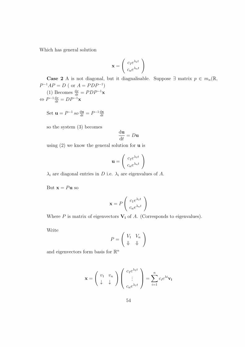
Which has general solution
x =
(c1e
λ1t
cneλnt
)Case 2 A is not diagonal, but it diagnalisable. Suppose ∃ matrix p ∈ mn(R,
P−1AP = D ( or A = PDP−1)
(1) Becomes dxdt
= PDP−1x
⇔ P−1 dxdt
= DP−1x
Set u = P−1 so dudt
= P−1 dxdt
so the system (3) becomesdu
dt= Du
using (2) we know the general solution for u is
u =
(c1e
λ1t
cneλnt
)λi are diagonal entries in D i.e. λi are eigenvalues of A.
But x = Pu so
x = P
(c1e
λ1t
cneλnt
)Where P is matrix of eigenvectors Vi of A. (Corresponds to eigenvalues).
Write
P =
(V1 Vn
⇓ ⇓
)and eigenvectors form basis for Rn
x =
(v1 vn
↓ ↓
) c1eλ1t
...
cneλ1t
=n∑i=1
cieλivi
54

Theorem 14.1. LetA ∈Mn(R) the general solution of the matrix d.e.
dx
dt= Ax is x = etAc
where c ∈ Rn is arbitrary.
Proof.
dx
dt= Ax ↔ dx
dt− Ax = 0
↔ e−tA(dx
dt− Ax) = 0
↔ e−tAdx
dt− A︸ ︷︷ ︸
exact
e−tAx = 0
↔ d
dt(e−tAx) = 0
↔ e−tAx = c
↔ x = e−tAc
some c ∈Rn
So we have proved
Theorem 14.2. Suppose A ∈ mn(R) has n linear independent e-vectors correspond-
ing to eigenvalues λ1 . . . λn. Then the general solution of the linear system
dx
dt= Ax
is
x =n∑i=1
cieλitvi
where ci . . . cn are arbitrary constants.
55

Case 3 Suppose A is not a diagonalisable matrix. We can devise a solution using
the exponential matrix eA, where
eA = I + A+ 11A
2 + 131A3 + . . .. Considering Sn, sequence of partial sums of eA,
it can be shown that lin︸︷︷︸n→∞
sij, n exists
foralli, j, where sij, n is i, j entry of sn. Define xxx to be sum of p.s.
we need the following Lemma.
Lemma 14.3. Let A ∈Mn(R)
detA
dt= AetA; (14.1)
e−tA = (etA)−1 (14.2)
Proof P263 Kumpel and Thorpe. Linear Algebra
56