Linear Algebra I
252
Linear Algebra I Skills, Concepts and Applications Gregg Waterman Oregon Institute of Technology
Transcript of Linear Algebra I

Linear Algebra I
Skills, Concepts and Applications
Gregg Waterman
Oregon Institute of Technology

c©2016 Gregg Waterman
This work is licensed under the Creative Commons Attribution 4.0 International license. The essence of the licenseis that
You are free to:
• Share - copy and redistribute the material in any medium or format
• Adapt - remix, transform, and build upon the material for any purpose, even commercially.
The licensor cannot revoke these freedoms as long as you follow the license terms.
Under the following terms:
• Attribution - You must give appropriate credit, provide a link to the license, and indicate if changeswere made. You may do so in any reasonable manner, but not in any way that suggests the licensorendorses you or your use.
No additional restrictions - You may not apply legal terms or technological measures that legally restrictothers from doing anything the license permits.
Notices:
You do not have to comply with the license for elements of the material in the public domain or where youruse is permitted by an applicable exception or limitation.
No warranties are given. The license may not give you all of the permissions necessary for your intendeduse. For example, other rights such as publicity, privacy, or moral rights may limit how you use the material.
For any reuse or distribution, you must make clear to others the license terms of this work. The best wayto do this is with a link to the web page below.
To view a full copy of this license, visit https://creativecommons.org/licenses/by/4.0/legalcode.

Contents
1 Systems of Linear Equations 11.1 Linear Equations and Systems of Linear Equations . . . . . . . . . . . . . . . . . . . . . 21.2 Curve Fitting, Temperature Equilibrium and Electric Circuits . . . . . . . . . . . . . . . 71.3 Solving Systems of Linear Equations . . . . . . . . . . . . . . . . . . . . . . . . . . . . 131.4 Solving With Matrices . . . . . . . . . . . . . . . . . . . . . . . . . . . . . . . . . . . . 171.5 “When Things Go Wrong” . . . . . . . . . . . . . . . . . . . . . . . . . . . . . . . . . 251.6 Back to Applications . . . . . . . . . . . . . . . . . . . . . . . . . . . . . . . . . . . . 311.7 Chapter 1 Exercises . . . . . . . . . . . . . . . . . . . . . . . . . . . . . . . . . . . . . 35
2 Euclidean Space and Vectors 402.1 Euclidean Space . . . . . . . . . . . . . . . . . . . . . . . . . . . . . . . . . . . . . . . 412.2 Introduction to Vectors . . . . . . . . . . . . . . . . . . . . . . . . . . . . . . . . . . . 452.3 Addition and Scalar Multiplication of Vectors, Linear Combinations . . . . . . . . . . . . 482.4 Linear Combination Form of a System . . . . . . . . . . . . . . . . . . . . . . . . . . . 542.5 Sets of Vectors . . . . . . . . . . . . . . . . . . . . . . . . . . . . . . . . . . . . . . . . 582.6 Vector Equations of Lines and Planes . . . . . . . . . . . . . . . . . . . . . . . . . . . . 622.7 Interpreting Solutions to Systems of Linear Equations . . . . . . . . . . . . . . . . . . . 682.8 The Dot Product of Vectors, Projections . . . . . . . . . . . . . . . . . . . . . . . . . . 72
3 Matrices and Vectors 763.1 Introduction to Matrices . . . . . . . . . . . . . . . . . . . . . . . . . . . . . . . . . . 783.2 Matrix Times a Vector . . . . . . . . . . . . . . . . . . . . . . . . . . . . . . . . . . . 823.3 Actions of Matrices on Vectors: Transformations in R
2 . . . . . . . . . . . . . . . . . . 903.4 Multiplying Matrices . . . . . . . . . . . . . . . . . . . . . . . . . . . . . . . . . . . . . 943.5 Inverse Matrices . . . . . . . . . . . . . . . . . . . . . . . . . . . . . . . . . . . . . . . 1023.6 Determinants and Systems of Equations . . . . . . . . . . . . . . . . . . . . . . . . . . 1083.7 Applications: Transformation Matrices, Graph Theory . . . . . . . . . . . . . . . . . . . 115
4 Vector Spaces and Subspaces 1214.1 Span of a Set of Vectors . . . . . . . . . . . . . . . . . . . . . . . . . . . . . . . . . . 1224.2 Closure of a Set Under an Operation . . . . . . . . . . . . . . . . . . . . . . . . . . . . 1284.3 Vector Spaces and Subspaces . . . . . . . . . . . . . . . . . . . . . . . . . . . . . . . . 1314.4 Column Space and Null Space of a Matrix . . . . . . . . . . . . . . . . . . . . . . . . . 1384.5 Least Squares Solutions to Inconsistent Systems . . . . . . . . . . . . . . . . . . . . . . 1424.6 Linear Independence . . . . . . . . . . . . . . . . . . . . . . . . . . . . . . . . . . . . . 1474.7 Bases of Subspaces, Dimension . . . . . . . . . . . . . . . . . . . . . . . . . . . . . . . 1554.8 Bases for the Column Space and Null Space of a Matrix . . . . . . . . . . . . . . . . . 1604.9 Solutions to Systems of Equations . . . . . . . . . . . . . . . . . . . . . . . . . . . . . 1654.10 Chapter 4 Exercises . . . . . . . . . . . . . . . . . . . . . . . . . . . . . . . . . . . . . 168
5 Linear Transformations 1705.1 Transformations of Vectors . . . . . . . . . . . . . . . . . . . . . . . . . . . . . . . . . 1715.2 Linear Transformations . . . . . . . . . . . . . . . . . . . . . . . . . . . . . . . . . . . 1765.3 Linear Transformations and Matrices . . . . . . . . . . . . . . . . . . . . . . . . . . . . 1835.4 Compositions of Transformations . . . . . . . . . . . . . . . . . . . . . . . . . . . . . . 1865.5 Transformations and Homogeneous Coordinates . . . . . . . . . . . . . . . . . . . . . . 1905.6 An Introduction to Eigenvalues and Eigenvectors . . . . . . . . . . . . . . . . . . . . . 1975.7 Finding Eigenvalues and Eigenvectors . . . . . . . . . . . . . . . . . . . . . . . . . . . . 2025.8 Diagonalization of Matrices . . . . . . . . . . . . . . . . . . . . . . . . . . . . . . . . . 211
i

5.9 Solving Systems of Differential Equations . . . . . . . . . . . . . . . . . . . . . . . . . 214
A Index of Symbols 217
B Solutions to Exercises 219B.1 Chapter 1 Solutions . . . . . . . . . . . . . . . . . . . . . . . . . . . . . . . . . . . . . 219B.2 Chapter 2 Solutions . . . . . . . . . . . . . . . . . . . . . . . . . . . . . . . . . . . . . 221B.3 Chapter 3 Solutions . . . . . . . . . . . . . . . . . . . . . . . . . . . . . . . . . . . . . 229B.4 Chapter 4 Solutions . . . . . . . . . . . . . . . . . . . . . . . . . . . . . . . . . . . . . 235B.5 Chapter 5 Solutions . . . . . . . . . . . . . . . . . . . . . . . . . . . . . . . . . . . . . 241
ii

1 Systems of Linear Equations
Learning Outcome:
1. Solve systems of linear equations using Gaussian elimination, use systems oflinear equations to solve problems.
Performance Criteria:
(a) Determine whether an equation in n unknowns is linear.
(b) Set up a system of linear equations to find coefficients of a line or poly-nomial through a given set of points, or to model flow in a network orequilibrium temperatures in a solid object.
(c) Determine whether an n-tuple is a solution to a linear equation or asystem of linear equations.
(d) Solve a system of two linear equations by the addition method.
(e) Give the coefficient matrix and augmented matrix for a system of equa-tions.
(f) Determine whether a matrix is in row-echelon form. Perform, by hand,elementary row operations to reduce a matrix to row-echelon form.
(g) Determine whether a matrix is in reduced row-echelon form. Use tech-nology to reduce a matrix to reduced row-echelon form.
(h) For a system of equations having a unique solution, determine the so-lution from either the row-echelon form or reduced row-echelon form ofthe augmented matrix for the system.
(i) Use a calculator to solve a system of linear equations having a uniquesolution.
(j) Given the row-echelon or reduced row-echelon form of an augmentedmatrix for a system of equations, determine the leading variables andfree variables of the system.
(k) Given the row-echelon or reduced row-echelon form for a system of equa-tions:
• Determine whether the system has a unique solution, and give thesolution if it does.
• If the system does not have a unique solution, determine whether itis inconsistent (no solution) or dependent (infinitely many solutions).
• If the system is dependent, give the general form of a solution andgive some particular solutions.
(l) Use systems of equations to solve network problems.
1
1.1 Linear Equations and Systems of Linear Equations
Performance Criteria:
1. (a) Determine whether an equation in n unknowns is linear.
(b) Set up a system of linear equations to find coefficients of a line or poly-nomial through a given set of points, or to model flow in a network orequilibrium temperatures in a solid object.
(c) Determine whether an n-tuple is a solution to a linear equation or asystem of linear equations.
Linear Equations and Their Solutions
It is natural to begin our study of linear algebra with the process of solving systems of linear equations,and applications of such systems.
Definition 1.1.1: A linear equation in n unknowns is an equation that can beput in the form
a1x1 + a2x2 + a3x3 + · · ·+ anxn = b, (1)
where a1, a2, ..., an and b are known constants and x1, x2, ... , xn are unknownvalues. A solution to a linear equation is a collection of values for the unknownsthat makes the equation true.
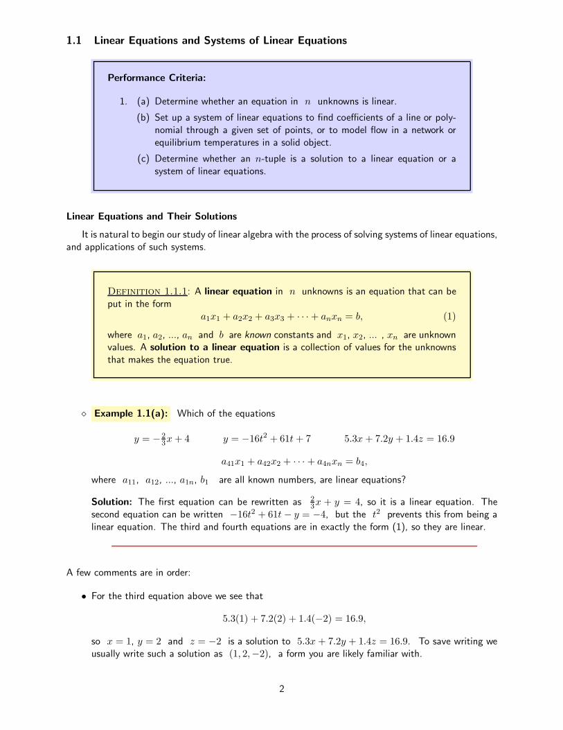
⋄ Example 1.1(a): Which of the equations
y = −23x+ 4 y = −16t2 + 61t+ 7 5.3x+ 7.2y + 1.4z = 16.9
a41x1 + a42x2 + · · · + a4nxn = b4,
where a11, a12, ..., a1n, b1 are all known numbers, are linear equations?
Solution: The first equation can be rewritten as 23x + y = 4, so it is a linear equation. The
second equation can be written −16t2 + 61t− y = −4, but the t2 prevents this from being alinear equation. The third and fourth equations are in exactly the form (1), so they are linear.
A few comments are in order:
• For the third equation above we see that
5.3(1) + 7.2(2) + 1.4(−2) = 16.9,
so x = 1, y = 2 and z = −2 is a solution to 5.3x + 7.2y + 1.4z = 16.9. To save writing weusually write such a solution as (1, 2,−2), a form you are likely familiar with.
2

• The equation y = −23x+4 can also be rewritten as 2x+3y = 12 instead of 2
3x+ y = 4. An(x, y) pair that is a solution to any one of the forms is also a solution to the other two (and anypair that is NOT a solution to any one of them will not be a solution to the other two either).We can multiply or divide both sides of a linear equation by a value in order to make it easier towork with, if we wish.
• Although you may have used x and y, or x, y and z as the unknown quantities in thepast, like in the third equation above, we will often use x1, x2, ..., xn instead. Thus the thirdequation could be written
5.3x1 + 7.2x2 + 1.4x3 = 15.9,
which is equivalent to the fourth equation with a41 = 5.3, a42 = 7.2, a43 = 1.4 and b4 = 15.9.One obvious advantage to using the letter a for all of the numbers is that we don’t have to fretabout what letters to use, and there is no danger of running out of letters! You will eventuallysee that there is also a very good mathematical reason for using just x (or some other singleletter), with subscripts denoting different values.
It is important that you easily recognize the form (1) from the definition of a linear equation. Soonwe will be interested in similar equations, but of the form
number · vector + number · vector + · · · + number · vector = vector.
We now move on to the concept that forms the beginning of our study of linear algebra:
Definition 1.1.2: A system of linear equations is a set of linear equationscontaining the same unknowns. (Not every equation needs to contain every un-known.) A solution to a system of linear equations is a collection of values forthe unknowns that makes every equation of the system true.
⋄ Example 1.1(b): Which of the following are systems of linear equations?
x+ 3y − 2z = −43x+ 7y + z = 4
−2x+ y + 7z = 7
x+ y2 = 3
x2 + y2 = 5
4t1 − t2 − t3 = 108
−t1 + 4t2 − t4 = 106
−t1 + 4t3 − t4 = 94
−t2 − t3 + 4t4 = 96
Solution: The first and third systems are systems of linear equations, the second is not. Thesecond is a system of nonlinear equations. One can verify that (3,−1, 2) is a solution to thefirst system of equations.
Here we note the following:
• The first system in the previous example is a system of three equations in three unknowns. Wewill spend a lot of time with such systems because they exhibit just about everything that wewould like to see but are small enough to be manageable to work with. As noted before, we willoften use x1, x2 and x3 instead of x, y and z for the unknowns.
3

• The numbers that the unknowns are multiplied by are coefficients of the system. It is customaryto get the coefficient/unknown terms on the left, and the numbers not multiplying an unknownon the right, as shown in the first and third (and second, for that matter) examples above. Thenumbers without unknowns are often referred to as the “right hand sides.”
• One should note carefully the coefficients of the third system and howthey are arranged, as shown to the right. Later we will put some bracketsaround such an array and call it a matrix. The fours are on what we willcall the diagonal of the matrix. (It seems that there is another diagonalwith zeros on it, but that diagonal, from lower left to upper right, hasno real significance. We therefore make no special note of what is going
4 −1 −1 0
−1 4 0 −1−1 0 4 −10 −1 −1 4
on there.) In addition to noting the fours on the diagonal, we also need to make special note ofthe way that the zeros and negative ones are arranged symmetrically across the diagonal. Thatsort of pattern is commonly encountered in physical applications of systems of linear equations.
• When discussing a system of linear equations in general, we often use the following notation, givenfor a system of m equations in n unknowns:
a11x1 + a12x2 + · · ·+ a1nxn = b1
a21x1 + a22x2 + · · ·+ a2nxn = b2...
...
am1x1 + am2x2 + · · ·+ amnxn = bm
(2)
Here the aijs are the coefficients, with the first subscript of each giving the equation and thesecond subscript giving which unknown x1, x2, ... it is with.
Systems of equations arise naturally in many engineering applications (as well as applications inother areas like business). Some of the uses of systems of equations that we’ll work with are
• analysis of electric circuits
• equilibrium distribution of heat in solid materials
• stress and strain in solid materials
• linear regression (least-squares approximation)
You will begin exploring some of these applications in the exercises for this section and the next. Thereare applications of other linear algebra concepts that we’ll see later, such as
• robotics and computer graphics
• sports and internet search rankings
• air travel routing
• signal processing
4

Section 1.1 Exercises To Solutions
1. Which of the following equations are linear equations?
(a) 4x2 + 3y2 = 5 (b)t1 + t2 + 83
4= t3 (c) 3x1 − x2 + 4x3 = x2
(d) 4.3 = 1.7m + b (e) y =√10− x (f)
5
x+
2
y= 7
2. Which of the systems of equations below are linear?
x1 − x2 + x3 = 3
2x1 − x2 + 4x3 = 7
3x1 − 5x2 − x3 = 7
3x+ y − 2z = −45x + 4z = 3
x− y + 2z = 0
x2 − y = 3
x− y = 1
3. (a) Determine which of the following are solutions to the first system of equations in the previousexercise: (5,−2, 4), (−2,−3, 2), (7, 3, 1)
(b) Determine which of the following are solutions to the second system of equations in theprevious exercise: (3,−19,−3), (−1, 3, 2), (5,−2, 4)
(c) Determine which of the following are solutions to the third system of equations in the previousexercise: (2, 1), (3, 5), (−1,−2)
4. Consider the equation y = ax3 + bx2 + cx+ d, representing a third degree polynomial.
(a) Substitute the value −2 for x and 5 for y into y = ax3 + bx2 + cx+ d, and simplifythe result. Is the resulting equation linear?
(b) Substitute the values a = 7, b = −2, c = −5 and d = 1 into y = ax3 + bx2 + cx+ d.Is the resulting equation linear?
5. It turns out that there is exactly one third degree polynomial with equation y = ax3 + bx2 +cx+ d whose graph goes through the four points
(−2, 5) (−1, 2) (1, 3) (3, 0)
Substitute each of those pairs into the equation (one pair at a time) to obtain four equations inthe four unknowns a, b, c and d. Give your final system in the form (2). Once we know howto solve such a system we can determine the values of a, b, c and d.
4
4x
y
6. The graph to the right shows a plot of the five points withcoordinates
(1.2, 3.7) (2.5, 4.1) (3.2, 4.7) (4.3, 5.2) (5.1, 5.9).
You can see that there is no line containing them, but the pointsare arranged somewhat linearly. In many applications it is de-sirable to find the line that comes closest (in a sense to bedescribed later) to passing through all of the points. Substituteeach of the points individually into the equation y = mx+b toobtain a system of five equations. (What are the unknowns?)Give the system in the form (2).
5

f1f4
f3 f2
n1n3
n4
n2
8
4
1
5
7. In many engineering applications we are interested in flowthrough a network. The flow could consist of water or airthrough pipes or ductwork (mechanical engineering), electronsthrough a circuit (or current, electrical engineering) or automo-biles on a raodway (civil engineering). Such a network can bemodeled by a set of nodes or vertices connected by arcs orline segments, typically called edges. The guiding principle formost such networks is simple: the flow into any node must equalthe flow out. The network to the right represents a traffic circle.The numbers next to each of the paths leading into or out of thecircle are the net flows in the directions of the arrows, in vehiclesper minute, during the first part of lunch hour. The unknownsf1, f2, f3 and f4 represent the flows in the corresponding arcsof the traffic circle.
(a) The nodes of the network have been labeled n1, n2, n3 and n4. At node n1, “flowin equals flow out” gives us f1 = f2 + 5. Rearranging this to get the unknowns on oneside with f1 positive, we get f1 − f2 = 5. Repeat at nodes n2, n3 and n4, withthe corresponding flows being positive in each case. That is, f2 should be positive in theequation obtained at n2, and so on. Give the resulting system of equations.
(b) Determine which of the following “4-tuples” (an n-tuple is an ordered “tuple” or collectionof values, separated by commas) are solutions to the system that you obtained. Note thatthis illustrates that a system can have more than one solution.
(12, 7, 8, 4) (7, 2, 3,−1) (10, 5, 6, 2) (9, 4, 3, 1)
(c) Which of the 4-tuples that you found to be a solution to your system would cause a problemwith the traffic circle? Explain.
(d) Suppose that f3 = 9. Just by looking at the traffic circle and using the “flow in equalsflow out, determine the other three flows.
6
1.2 Curve Fitting, Temperature Equilibrium and Electric Circuits
Performance Criterion:
1. (b) Set up a system of linear equations to find coefficients of a line or poly-nomial through a given set of points, or to model flow in a network orequilibrium temperatures in a solid object.
Curve Fitting
Curve fitting refers to the process of finding a polynomial function of “minimal degree” whose graphcontains some given points. We all know that any two distinct points (that is, points that are not thesame) in R
2 have exactly one line through them. In a previous course you should have learned how tofind the equation of that line in the following manner. Suppose that we wish to find the equation of theline through the points (2, 3) and (6, 1). We know that the equation of a line looks like y = mx + b,
where m and b are to be determined. m is the slope, which can be found by m =3− 1
2− 6=
2
−4 = −12 .
Therefore the equation of our line looks like y = −12x + b. To find b we simply substitute either of
the given ordered pairs into our equation (the fact that both pairs lie on the line means that either pairis a solution to the equation) and solve for b: 3 = −1
2(2) + b =⇒ b = 4. The equation of the linethrough (2, 3) and (6, 1) is then y = −1
2x+ 4.We will now solve the same problem in a different way. A student should understand that whenever
a new approach to a familiar exercise is taken, there is something to be gained by it. Usually the newmethod is in some way more powerful, and allows the solving of additional problems. This will be thecase with the following example, which uses a process you should have seen in a previous course, andthat we will review in detail in the next section.
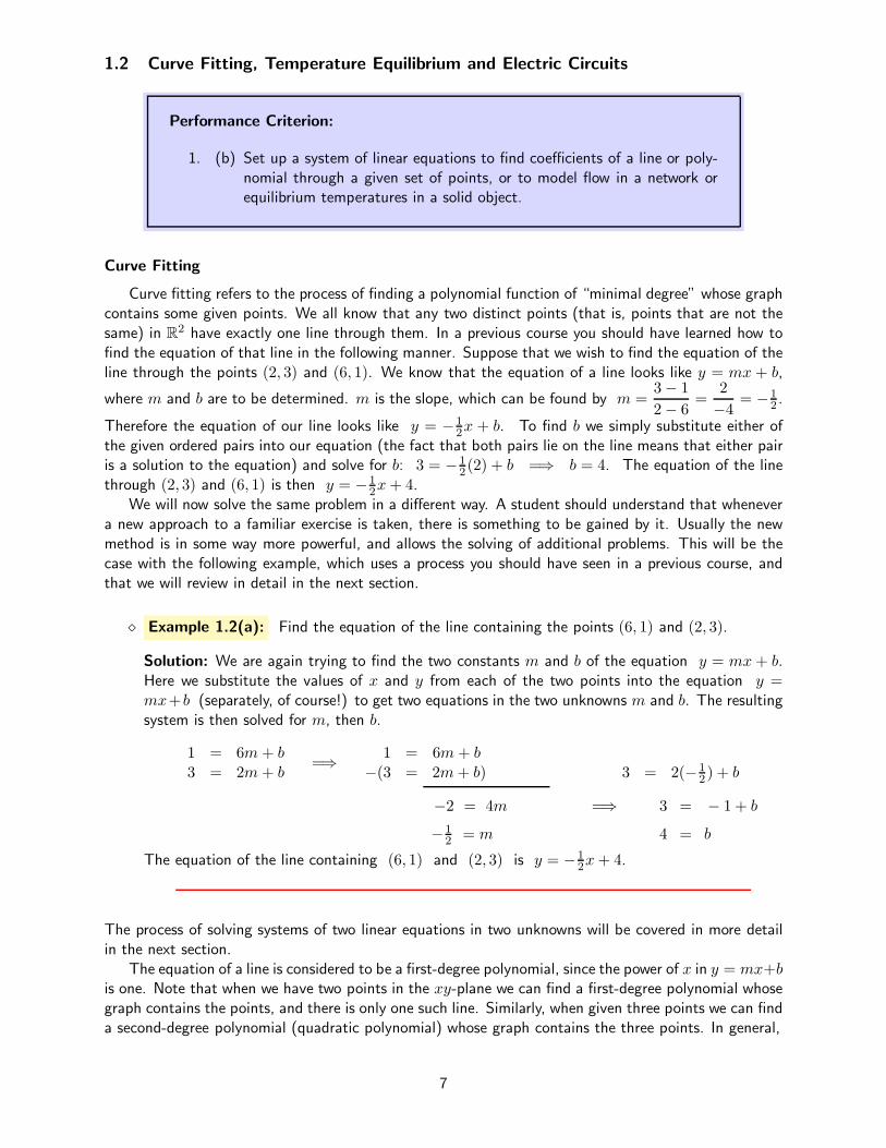
⋄ Example 1.2(a): Find the equation of the line containing the points (6, 1) and (2, 3).
Solution: We are again trying to find the two constants m and b of the equation y = mx+ b.Here we substitute the values of x and y from each of the two points into the equation y =mx+b (separately, of course!) to get two equations in the two unknowns m and b. The resultingsystem is then solved for m, then b.
1 = 6m+ b
3 = 2m+ b=⇒ 1 = 6m+ b
−(3 = 2m+ b) 3 = 2(−12 ) + b
−2 = 4m =⇒ 3 = − 1 + b
−12 = m 4 = b
The equation of the line containing (6, 1) and (2, 3) is y = −12x+ 4.
The process of solving systems of two linear equations in two unknowns will be covered in more detailin the next section.
The equation of a line is considered to be a first-degree polynomial, since the power of x in y = mx+b
is one. Note that when we have two points in the xy-plane we can find a first-degree polynomial whosegraph contains the points, and there is only one such line. Similarly, when given three points we can finda second-degree polynomial (quadratic polynomial) whose graph contains the three points. In general,
7

Theorem 1.2.1: Given n points in the plane such that (a) no two of themhave the same x-coordinate and (b) they are not collinear, we can find a uniquepolynomial function of degree n− 1 whose graph contains the n points.
Often in mathematics we are looking for some object (solution) and we wish to be certain that suchan object exists. In addition, it is generally preferable that only one such object exists. We refer tothe first of these wishes as “existence,” and the second is “uniqueness.” If we have, for example, fourpoints meeting the two conditions of the above theorem, there would be infinitely many fourth degreepolynomials whose graphs would contain them, and the same would be true for fifth degree, sixth degree,and so on. Additionally, a set of four points meeting the above conditions will likely NOT not have apolynomial of degree two whose graph passes through all of them. But the theorem guarantees us thatthere is one, and only one, third degree polynomial whose graph contains the four points. In Exercise3 of the previous section you saw how to construct a system of linear equations whose solution givesus the coefficients of the third degree polynomial whose graph contains four given points. In Example1.4(e) we’ll see how to find such a polynomial, from start to finish.
Temperature Equilibrium
Consider the following hypothetical situation: We have a plate of metal that is perfectly insulatedon both of its faces so that no heat can get in or out of the faces. Each point on the edge (which we willcall the boundary), however, is held at a constant temperature (constant at that point, but possiblydiffering from point to point). The temperatures at points on the boundary affect the temperatures atinterior points. If the plate is left alone for a long time (“infinitely long”), the temperature at each pointin the interior of the plate will reach a constant temperature, called the “equilibrium temperature.” Thisequilibrium temperature at any given interior point is a weighted average of the temperatures at allthe boundary points, with temperatures at closer boundary points being weighted more heavily in theaverage than the temperatures at boundary points that are farther away.
The task of trying to determine those interior temperatures based on the edge temperatures isa famous problem of applied mathematics, called the Dirichlet problem (pronounced “dir-i-shlay”).Finding the exact solution involves methods beyond the scope of this course, but we will use systems ofequations to solve the problem “numerically,” which means to approximate the exact solution, usuallyby some non-calculus method. The key to solving the Dirichlet problem is the following:
Theorem 1.2.2: Mean Value Property
The equilibrium temperature at any interior point P is the average of the temper-atures of all interior points on any circle centered at P .
We will solve what are called discrete versions of the Dirichlet problem, which means that we onlyknow the temperatures at a finite number of points on the boundary of our metal plate, and we willonly find the equilibrium temperatures at a finite number of the interior points. These finite points,both on the boundary and in the interior, are usually evenly spaced on a rectangular grid. Considerthe plate shown in Figure 1.2(a) on the next page, with boundary temperatures known at the indicatedpoints. We can then construct a square grid in the interior of the plate, as shown in Figure 1.2(b). Theunknown temperatures at the mesh points of the grid are denoted by t1, t2, t3 and t4, as shownin Figure 1.2(b). By the mean value property, the temperature t1 is the average of the temperaturesat all points on the circle shown in Figure 1.2(c). Such an average is obtained by an integral, but in
8

our case we will simply average the temperatures at the four boundary and mesh points that are on thecircle. This gives us the equation
t1 =61 + 68 + t2 + t3
4.
68 65
53 50
61 59
55 52
Figure 1.2(a)
t1 t2
t3 t4
68 65
53 50
61 59
55 52
Figure 1.2(b)
t1 t2
t3
t4
68 65
53 50
61 59
55 52
Figure 1.2(c)
We can then find three more such equations for circles centered at the mesh points with temperaturest2, t3 and t4. If we then multiply both sides of each equation by four, combine the two knownnumerical values and get all of the unknowns on one side of each equation, we can obtain a system oflinear equations in the standard form. You will do this in the exercises at the end of the section.
Electric Circuits
We could spend a great deal of time that we don’t have on electric circuits, so here we’ll justlearn one method to get a system of linear equations modeling a circuit with constant voltage sources(batteries) and resistors. An example of such a circuit is shown below and to the left. The lines indicatewires that are connected at the dots, which are called principal nodes, and the portion of the circuitbetween two principle nodes we’ll call a branch. A set of branches that can be placed end to end toget from one node back to itself is called a loop.
+
−
+
−V1
V2
R1
R2
R3
R4
R5
+
−
+
−I1
I2
I3
V1
V2
R1
R2
R3
R4
R5
Each “zig-zag” is a resistor and the parallel long and short lines with + and − at either side arebatteries. Each resistor has a characteristic called its resistance, which is measured in ohms. Similarly,each battery has a voltage, measured in ... volts! We will let V1 and V2 represent both the voltagesources and their voltages, and R1 through R5 will represent both the indicated resistors and theirresistances.
The voltage sources cause something called current to flow in the circuit. Intuitively, we can thinkof the voltage sources as “pumps” pushing current through the wires, like pushing water through pipes.The resistors “resist” the flow of current. Our objective is to find the current in each branch of thecircuit. To find the current in each branch we will proceed as follows:
9

1) Establish a clockwise or counterclockwise direction of current in each loop. If there is a voltagesource in a loop, establish the current in the direction from the negative side to the positive side.If there is no voltage source, the current can be in either direction that you wish. (If you choosethe “wrong” direction you will simply obtain a negative value for the current.) The diagram aboveand to the right shows currents established for each loop - we will use I for current.
2) The “voltage drop” across each resistor is given by Ohm’s Law, V = IR. Kirchoff’s VoltageLaw then tells us that the voltage supplied in a loop is equal to the sum of the voltage drops acrosseach of the resistors in the loop. When working in a loop and calculating the voltage drop acrossa resistor shared with another loop, the current used is the one for the loop under considerationplus or minus the current from the adjacent loop, depending on whether that current is going thesame, or the opposite, direction as the current in the loop under consideration. Write an equationfor each loop based on Kirchoff’s Voltage Law. If there is no voltage source in a loop, the voltagesupplied is zero.
3) Get each equation in the form aI1 + bI2 + cI3 = Vk, where k is the loop the equation wasobtained from.
4) Solve the system of equations.
In Section 1.4 we’ll see how to solve such systems; for now we will only complete steps 1, 2 and 3 above.
⋄ Example 1.2(b): Use the steps above to obtain a system of three equations that models thecircuit shown below and to the right.
+
−
+
−I1
I2
I3
V1
V2
R1
R2
R3
R4
R5
Solution: For the loop with current I1 the voltagesupplied is V1. Going around the loop from thebattery the voltage drops are
I1R1, (I1 + I2)R4, (I1 − I3)R3.
Kirchoff’s Voltage Law then gives us
I1R1 + (I1 + I2)R4 + (I1 − I3)R3 = V1.
The equations for the other two loops are
I2R2 + (I2 + I1)R4 + (I2 + I3)R5 = 0
and(I3 − I1)R3 + (I3 + I2)R5 = V2.
Putting each of our three equations in the form aI1 + bI2 + cI3 = Vk gives us
(R1 +R3 +R4)I1 + R4I2 − R3I3 = V1
R4I1 + (R2 +R4 +R5)I2 + R5I3 = 0
− R3I1 + R5I2 + (R3 +R5)I3 = V2
10

It is worth noting the array of coefficients of the three unknowns I1, I2 and I3:
R1 +R3 +R4 R4 −R3
R4 R2 +R4 +R5 R5
−R3 R5 R3 +R5
Once again we see symmetry across the diagonal!Let’s do another example with numerical values for the voltage and resistances:
⋄ Example 1.2(c): Find a system of equations that models the circuit below and to the right.
Solution: Here we establish the current I1 in a coun-terclockwise direction in the left loop, and I2 in aclockwise direction in the right loop, as shown in thelower picture to the right. For the left loop we get theequation
(I1 + I2)10 + 20I1 = 12
and, from the right loop,
30I2 + (I2 + I1)10 = 6.
Distributing the resistances and regrouping gives us thesystem
30I1 + 10I2 = 12
10I1 + 40I2 = 6
−+
−+
12V 6V
20Ω
10Ω
30Ω
−+
−+
I1 I212V 6V
20Ω
30Ω
Section 1.2 Exercises To Solutions
1. Consider the four points (−1, 3), (1, 5), (2, 4) and (4,−1). By Theorem 1.2.1, there is a uniquethird degree polynomial of the form
y = a+ bx+ cx2 + dx3 (1)
whose graph contains those four points.
(a) Substitute the x and y values from the first ordered pair into (1) and rearrange theresulting equation so that it has all of the unknowns on the left and a number on the right,like all of the linear equations we have worked with so far.
(b) Repeat (a) for the other 3 ordered pairs, and give the system of equations whose solution isthe four coefficients a, b, c and d.
2. Give a system of equations that can be solved to find the values of a, b and c for the quadraticpolynomial y = ax2 + bx+ c whose graph is the parabola passing through the points (−1,−4),(1, 1) and (3, 0).
11

t1 t2
t3 t4
68 65
53 50
61 59
55 52
3. To the right is a diagram of the metal plate described in the discussionof the mean value property for temperature equilibrium. In this exerciseyou will set up a system of equations whose solution gives the unknowntemperatures t1, t2, t3 and t4 at the four interior points.
(a) Applying the mean value property at the mesh point with temper-
ature t1 gave us the equation t1 =61 + 68 + t2 + t3
4. Multiply
both sides by four to eliminate the fraction, subtract t2 andt3 from both sides and add 61 and 68. You should end up withan equation of the form at1 + bt2 + ct3 + dt4 = e, where d = 0.
(b) Follow a similar process for each of the other three interior mesh points in order to obtaina system of four equations in the four unknowns t1, t2, t3 and t4. In each equation oneof a, b, c or d will be zero, so each equation will actually only contain three of t1, t2,t3 and t4.
(c) Although we can put the four equations in any order we want, arrange them so that thecoefficients of four are along the diagonal of the left side, as we saw in third system ofExample 1.1(b). Be sure that the remaining coefficients are symmetric about the diagonal.If they are not, find and correct your error.
4. (a) Give the system of equations modeling the circuit below and to the left.
(b) Give the system of equations modeling the circuit below and to the right.
+
−I1
I2
I3
20V
5Ω
10Ω
6Ω
8Ω
2Ω
1Ω
A
C B
Exercise 4(a)
+
−
+−
I1
I2
I3
12V
8V
4Ω
12Ω
8Ω
5Ω
2Ω
3Ω
Exercise 4(b)
(c) The solution to the circuit for Exercise 4(a) is I1 = 1.36 amperes, I2 = 0.39 amperes andI3 = 0.81 amperes. Given this information, what is the current in the branch from pointA to point C? (Note that it is I1 and I2 combined, with the direction of each takeninto account.) Does the current flow from A to C, or from C to A?
(d) Again considering the circuit for Exercise 4(a) with the current values given above, what isthe current in the branch from point B to point C? Does the current flow from B toC, or from C to B?
12

1.3 Solving Systems of Linear Equations
Performance Criteria:
1. (d) Solve a system of two linear equations by the addition method.
Now that we know some applications of systems of equations, and how to set up systems for anapplication, it is time we learn how to solve a system. In this section we remember how to solve asystem of two equations in two unknowns by the addition method, and extend the method to a systemof three equations in three unknowns. Then in Section 1.4, we will introduce the method that we willuse throughout the rest of the course.
Consider the systemx− 3y = 6
−2x+ 5y = −5 of linear equations. In this case a solution to the system
is an ordered pair (x, y) that makes both equations true. In the past you should have learned twomethods for solving such systems, the addition method and the substitution method. The methodwe want to focus on is the addition method. In this case we could multiply the first equation by two
and add the resulting equation to the second. The result isx− 3y = 6−y = 7
; from this we can see
that y = −7. This value is then substituted into the first equation to get x = −15.Sometimes we have to do something a little more complicated:
⋄ Example 1.3(a): Solve the system2x− 4y = 183x+ 5y = 5
using the addition method.
Solution: Here we can eliminate x by multiplying the first equation by 3 and the second by−2, then adding:
2x− 4y = 183x+ 5y = 5
=⇒ 6x− 12y = 54−6x− 10y = −10
−22y = 44
y = −2Now we can substitute this value of y back into either equation to find x:
2x− 4(−2) = 182x+ 8 = 18
2x = 10x = 5
The solution to the system is then x = 5, y = −2, which we usually write as the ordered pair(5,−2). It can be easily verified that this pair is a solution to both equations.
Let’s now solve an applied problem that uses a system of two equations.
13

⋄ Example 1.3(b): The temperatures (in degrees Fahrenheit) at sixpoints on the edge of a rectangular plate are shown to the right. As-suming that the temperatures in the plate have reached equilibrium, findthe interior temperatures t1 and t2 at their indicated “mesh points.”
t1
t2
15
15
60
45
45
30
Solution: The discrete version of the mean value property tells us that the equilibrium temperatureat any interior point of the mesh is the average of the four adjacent points. This gives us the twoequations
t1 =15 + 45 + 60 + t2
4and t2 =
15 + t1 + 45 + 30
4
If we multiply both sides of each equation by four, combine the constants and get the t1 and
t2 terms on the left side we get the system of equations4t1 − t2 = 120−t1 + 4t2 = 90
. Multiplying the
first equation by four and adding the result to the second gives us 15t1 = 570, from which wefind that t1 = 38. Substituting that into either equation and solving for t2 gives t2 = 32.These values can easily be shown to verify our discrete mean value property:
15 + 45 + 60 + t2
4=
15 + 45 + 60 + 32
4= 38 = t1 ,
15 + t1 + 45 + 30
4=
15 + 38 + 45 + 30
4= 32 = t2
Geometric Interpretation
At the start of this section we saw that the systemx− 3y = 6
−2x+ 5y = −5 has the solution (−15,−7).You should be aware that if we graph the equation x−3y = 6 we get a line. Technically speaking, whatwe have graphed is the solution set, the set of all pairs (x, y) that make the equation true. Any pair(x, y) of numbers that makes the equation true is on the line, and the (x, y) representing any pointon the line will make the equation true. If we plot the solution sets of both equations in the system
x− 3y = 6−2x+ 5y = −5 together in the coordinate plane we will get two lines. Since (−15,−7) is
a solution to both equations, the two lines cross at the point with those coordinates! We could usethis idea to (somewhat inefficiently and possibly inaccurately) solve a system of two equations in twounknowns:
⋄ Example 1.3(c): Solve the system2x− 3y = −63x− y = 5
graphically.
Solution: We begin by solving each of the equations for y; this will give us the equations iny = mx+ b form, for easy graphing. The results are
y = 23x+ 2 and y = 3x− 5
14

If we graph these two equations on the same graph, we get thepicture to the right. Note that the two lines cross at the point(3, 4), so the solution to the system of equations is (3, 4), orx = 3, y = 4.
5
5
-5
-5
y = 2
3x+ 2
y = 3x− 5
(3, 4)
x
y
It is possible that two lines in the standard two-dimensional plane might be parallel; in that case asystem consisting of the two equations representing those lines will have no solution. It is also possiblethat two equations might actually represent the same line, in which case the system consisting of thosetwo equations will have infinitely many solutions. Investigation of those two cases will lead us to morecomplex considerations that we will avoid for now.
A System of Equations in Three Unknowns
The previous examples were two linear equations with two unknowns. Now we consider the followingsystem of three linear equations in three unknowns.
x+ 3y − 2z = −43x+ 7y + z = 4
−2x+ y + 7z = 7
(1)
We can use the addition method here as well; first we multiply the first equation by negative three andadd it to the second. We then multiply the first equation by two and add it to the third. This eliminatesthe unknown x from the second and third equations, giving the second system of equations shownbelow. We can then add 7
2 times the second equation to the third to obtain a new third equationin which the unknown y has been eliminated. This “final” system of equations is shown to the rightbelow.
x+ 3y − 2z = −43x+ 7y + z = 4
−2x+ y + 7z = 7
=⇒x+ 3y − 2z = −4−2y + 7z = 16
7y + 3z = −1=⇒
x+ 3y − 2z = −4−2y + 7z = 16
552 z = 55
(2)
Above we have three different systems, each with three equations. The three systems are equivalent,meaning that a solution to any one of them is also a solution to the other two. The point of the aboveprocess is to obtain a system that is equivalent to the original but easier to solve. We can see that thesolution to the last equation of the third system is z = 2. That result is then substituted into thesecond equation in the last system to get y = −1. Finally, we substitute the values of y and z intothe first equation to get x = 3. The solution to the system is then the ordered triple (3,−1, 2).The process of finding the last unknown first, substituting it to find the next to last, and so on, is calledback substitution. The word “back” here means that we find the last unknown (in the order theyappear in the equations) first, then the next to last, and so on.
You might note that we could eliminate any of the three unknowns from any two equations, thenuse the addition method with those two to eliminate another variable. However, we will always follow aprocess that first uses the first equation to eliminate the first unknown from all equations but the first
15

one itself. After that we use the second equation to eliminate the second unknown from all equationsfrom the third on, and so on. One reason for this is that if we were to create a computer algorithm tosolve systems, it would need a consistent method to proceed, and what we have done is as good as any.
What is the geometric interpretation of this? Since there are three unknowns, the appropriategeometric setting is three-dimensional space. The solution set to any equation ax+ by + cz = d is aplane in three-dimensional space, as long as not all of a, b and c are zero. Therefore, a solution tothe system is a point that lies on each of the planes representing the solution sets of the three equations.For our example, then, the planes representing the three equations intersect at the point (3,−1, 2).
In the study of linear algebra we will be defining new concepts and developing corresponding notation.We begin the development of notation with the following. The set of all real numbers is denoted byR, and the set of all ordered pairs of real numbers is R
2, spoken as “R-two.” Geometrically, R2 is
the familiar Cartesian coordinate plane. Similarly, the set of all ordered triples of real numbers is thethree-dimensional space referred to as R
3, “R-three.”All of the algebra that we will be doing using equations with two or three unknowns can easily be
done with more unknowns. In general, when we are working with n unknowns, we will get solutionsthat are n-tuples of numbers. Any such n-tuple represents a location in n-dimensional space, denotedRn. Note that a linear equation in two unknowns represents a line in R
2, in the sense that the set ofsolutions to the equation forms a line. We consider a line to be a one-dimensional object, so the linearequation represents a one-dimensional object in two-dimensional space. The solution set to a linearequation in three unknowns is a plane in three-dimensional space. The plane itself is two-dimensional,so we have a two-dimensional “flat” object in three dimensional space.
Similarly, when we consider the solution set of a linear equation in n unknowns, its solution setrepresents an n − 1-dimensional “flat” object in n-dimensional space. When such an object has morethan two dimensions, we usually call it a hyperplane. Although such objects can’t be visualized, theycertainly exist in a mathematical sense.
Section 1.3 Exercises To Solutions
1. Solve each of the following systems by the addition method.
(a)2x− 3y = −7−2x+ 5y = 9
(b)2x− 3y = −63x− y = 5
(c)4x+ y = 14
2x+ 3y = 12
(d)7x− 6y = 13
6x− 5y = 11(e)
5x+ 3y = 7
3x− 5y = −23(f)
5x− 3y = −117x+ 6y = −12
2. Solve each of the following systems by graphing, as done in Example 1.3(c).
(a)3x− 4y = 8
x+ 2y = 6(b)
4x− 3y = 9
x+ 2y = −6(c)
5x+ y = 12
7x− 2y = 10
16

1.4 Solving With Matrices
Performance Criteria:
1. (e) Give the coefficient matrix and augmented matrix for a system of equa-tions.
(f) Determine whether a matrix is in row-echelon form. Perform, by hand,elementary row operations to reduce a matrix to row-echelon form.
(g) Determine whether a matrix is in reduced row-echelon form. Use tech-nology to reduce a matrix to reduced row-echelon form.
(h) For a system of equations having a unique solution, determine the so-lution from either the row-echelon form or reduced row-echelon form ofthe augmented matrix for the system.
(i) Use a calculator to solve a system of linear equations having a uniquesolution.
Note that when using the addition method for solving the system of three equations in three un-knowns in the previous section, the symbols x, y and z and the equal signs are simply “placeholders”that are “along for the ride.” To make the process cleaner we can simply arrange the constants a, b,c and d for each equation ax + by + cz = d in an array form called a matrix, which is simply atable of values like
1 3 −2 −43 7 1 4−2 1 7 7
. (1)
Each number in a matrix is called an entry of the matrix. Each horizontal line of numbers in a matrix isa row of the matrix, and each vertical line of numbers is a column. The size or dimensions of a matrixis (are) given by first telling the number of rows, then the number of columns, with the × symbolbetween them. The size of the above matrix is 3× 4, which we say as “three by four.”
Suppose that the above matrix came from the system of equations
x+ 3y − 2z = −43x+ 7y + z = 4
−2x+ y + 7z = 7
When a matrix represents a system of equations, as (1) does, it is called the augmented matrix of thesystem. The matrix consisting of just the coefficients of x, y and z from each equation is called thecoefficient matrix:
1 3 −23 7 1−2 1 7
We are not interested in the coefficient matrix at this time, but we will be later. The reason for thename “augmented matrix” will also be seen later.
Once we have the augmented matrix, we can perform a process called row-reduction, which isessentially what we did in the previous section, but we work with just the matrix rather than the systemof equations. The following example shows how this is done for the above matrix.
17

⋄ Example 1.4(a): Solve the system
x+ 3y − 2z = −43x+ 7y + z = 4
−2x+ y + 7z = 7
from the previous section by
row-reduction.
Solution: We begin with the augmented matrix for the system, shown below and to the left. Wethen add negative three times the first row to the second, and put the result in the second row.Then we add two times the first row to the third, and place the result in the third. Using thenotation Rn (not to be confused with R
n!) to represent the nth row of the matrix, we cansymbolize these two operations as shown in the middle below. The matrix to the right below isthe result of those operations.
1 3 −2 −43 7 1 4−2 1 7 7
−3R1 +R2 → R2
=⇒2R1 +R3 → R3
1 3 −2 −40 −2 7 160 7 3 −1
Next we finish with the following:
1 3 −2 −40 −2 7 160 7 3 −1
72R2 +R3 → R3
=⇒
1 3 −2 −40 −2 7 160 0 55
2 55
The process just outlined is called row reduction. At this point we return to the equation form
x+ 3y − 2z = −40x− 2y + 7z = 16
0x+ 0y + 552 z = 55
and perform back-substitution. The last equation gives us that z = 2. We can than substitutethis value into the second equation to get −2y + 14 = 16, resulting in y = −1. These valuesof y and z are substituted into the first equation which is then solved to get x = 3. Thesolution to the system is then (3,−1, 2).
The final form of the matrix before we went back to equation form is something called row-echelonform. (The word “echelon” is pronounced “esh-el-on.”) The first non-zero entry in each row is called aleading entry; in this case the leading entries are the numbers 1, −2 and 55
2 . To be in row-echelonform means that
• any rows containing all zeros are at the bottom of the matrix and
• the leading entry in any row is to the right of any leading entries above it.
⋄ Example 1.4(b): Which of the matrices below are in row-echelon form?
1 3 −2 −40 0 3 −50 7 −10 −1
2 6 −1 9 50 0 −8 1 −30 0 0 0 2
7 −12 5 00 0 0 00 −5 1 8
Solution: The leading entries of the rows of the first matrix are 1, 3 and 7. Because the leadingentry of the third row (7) is not to the right of the leading entry of the second row (3), the
18

first matrix is not in row-echelon form. In the third matrix, there is a row of zeros that is not atthe bottom of the matrix, so it is not in row-echelon form. The second matrix is in row-echelonform.
Note that if we switch the second and third rows of the first and third matrices in the above example,which we are usually allowed to do, then both will then be in row-echelon form.
It is possible to continue with the matrix operations to obtain something called reduced row-echelon form, from which it is easier to find the values of the unknowns. The requirements for beingin reduced row-echelon form are the same as for row-echelon form, with the addition of the following:
• All leading entries are ones.
• The entries above any leading entry are all zero except perhaps in the last column.
Obtaining reduced row-echelon form requires more matrix manipulations, and nothing is really gainedby obtaining that form if you are doing this by hand. However, when using software or a calculator itis most convenient to obtain reduced row-echelon form. Here are two examples of matrices in reducedrow-echelon form:
1 0 0 30 1 0 −70 0 1 4
1 6 0 9 00 0 1 2 00 0 0 0 1
In the next section we will see how to interpret what the second matrix would be telling us if it camefrom a system of equations. The next example shows what the first matrix tells us.
⋄ Example 1.4(c): Suppose that the matrix to the right is the result ofrow-reduction of the augmented matrix for a system of three equations inthe unknowns x1, x2 and x3. Determine the values of the unknowns.
1 0 0 30 1 0 −70 0 1 4
Solution: When using row-reduction to solve a system we first create the augmented matrix forthe system, then row-reduce it, and then we go back to equations. The equations we would returnto for the above matrix are
1x1 + 0x2 + 0x3 = 30x1 + 1x2 + 0x3 = −70x1 + 0x2 + 1x3 = 4
and from these we can easily see the solution: x1 = 3, x2 = −7 and x3 = 4.
In practice, very large systems are solved by row-reduction. Many issues arise when doing this. Forexample, coefficients are often obtained from some sorts of measurements that give rounded values. Atevery step of row-reduction more rounding needs to take place, resulting in rounding errors. Additionally,matrices used in practice can have entries that cause introduction of other errors in the process of row-reduction. We could spend an entire course examining such concerns, but instead we’ll focus on lessnumerically oriented aspects of linear algebra.
That said, let’s look at one thing that can come up in the process of row-reduction, illustrated inthe following example.
19

⋄ Example 1.4(d): Row-reduce the matrix
1 3 −2 −42 6 −1 −13−1 4 −8 3
.
Solution: We begin by adding negative two times the first row to the second, and put the resultin the second row. Then we add two times the first row to the third, and place the result in thethird. Using the notation Rn (not to be confused with R
n!) to represent the nth row of thematrix, we can symbolize these two operations as shown in the middle below. The matrix to theright below is the result of those operations.
1 3 −2 −42 6 −1 −13−1 4 −8 3
−2R1 +R2 → R2
=⇒R1 +R3 → R3
1 3 −2 −40 0 3 −50 7 −10 −1
We can see that the matrix would be in row-echelon form if we simply switched the second andthird rows (which is equivalent to simply rearranging the order of our original equations), so that’swhat we do:
1 3 −2 −40 0 3 −50 7 −10 −1
R2 ←→ R3
=⇒
1 3 −2 −40 7 −10 −10 0 3 −5
The act of rearranging rows in a matrix is called permuting them. In general, a permutation of aset of objects is simply a rearrangement of them. When solving a system by row-reduction, permutingsimply amounts to changing the order of the original equations, and doing so will not affect the solutionto the system.
Row Reduction Using Technology
There are three main technologies that can be used to get an augmented matrix into reducedrow-echelon form:
• Most or all graphing calculators (and the TI-36X Pro, a non-graphing calculator) will perform rowreduction via the rref function. Do a search to find an article or video on how to rref with yourparticular model of calculator.
• There are numerous matrix calculators that can be found online - there is a link to one at theclass web page.
• Various mathematical software programs, like MATLAB, will perform row-reduction.
Now that we know how to solve systems of linear equations we can complete an application.
⋄ Example 1.4(e): Find the equation of the third degree polynomial containing the points
(−1,−7), (0, 1), (1, 5) and (2, 11).
Solution: A general third degree polynomial has an equation of the form y = ax3+bx2+cx+d;our goal is to find values of a, b, c and d so that the given points all satisfy the equation.Since the values x = −1, y = −7 must make the general equation true, we have −7 =
20

a(−1)3 + b(−1)2 + c(−1) + d = −a+ b− c+ d. Doing this with all four given ordered pairs and“flipping” each equation gives us the system
−a+ b− c+ d = −7d = 1
a+ b+ c+ d = 58a+ 4b+ 2c+ d = 11
If we enter the augmented matrix for this system in our calculators and rref we get
−1 1 −1 1 −70 0 0 1 11 1 1 1 58 4 2 1 11
rref=⇒
1 0 0 0 10 1 0 0 −20 0 1 0 50 0 0 1 1
So a = 1, b = −2, c = 5, d = 1, and the desired polynomial equation is y = x3− 2x2+5x+1.
Section 1.4 Exercises To Solutions
1. Give the coefficient matrix and augmented matrix for the system of equations
x + y − 3z = 1
−3x+ 2y − z = 7
2x+ y − 4z = 0
.
2. Determine which of the following matrices are in row-echelon form.
A =
[
3 −7 5 0 2 −40 0 0 −2 5 −1
]
B =
1 0 0 40 1 0 −20 0 1 5
C =
1 0 0 40 1 0 −20 0 3 5
D =
0 0 4 40 1 −3 26 1 3 5
E =
1 3 −5 10 −70 0 1 0 20 0 0 1 −40 0 0 0 10 0 0 0 0
F =
1 3 0 0 −70 0 1 0 20 0 0 1 −40 0 0 0 10 0 0 0 0
3. Determine which of the matrices in Exercise 2 are in reduced row-echelon form.
4. Perform the first two row operations for the augmented matrix from Exercise 1, to get zeros inthe bottom two entries of the first column.
5. Fill in the blanks in the second matrix with the appropriate values after the first step of row-reduction. Fill in the long blanks with the row operations used.
(a)
1 5 −7 3−5 3 −1 04 0 8 −1
=⇒
00
21

(b)
2 −8 −1 50 −2 0 00 6 −5 2
=⇒
00 0
(c)
1 −2 4 10 3 5 −20 2 −8 1
=⇒
00 0
6. Find x, y and z for the system of equations that reduces to each of the matrices shown.
(a)
1 6 −2 70 8 1 00 0 −2 8
(b)
1 6 −2 70 2 −5 −130 0 3 3
(c)
1 0 0 70 3 0 00 0 −4 8
7. Use row operations (by hand) on an augmented matrix to solve each system of equations.
(a)x− 2y − 3z = −12x+ y + z = 6x+ 3y − 2z = 13
(b)−x− y + 2z = 52x+ 3y − z = −35x− 2y + z = −10
(c)x+ 2y + 4z = 7−x+ y + 2z = 52x+ 3y + 3z = 7
8. Use the rref capability of your calculator to solve each of the systems from the previous exercise.
9. Temperatures at points along the edges of a rectangular plate are as shown below and to the left.Find the equilibrium temperature at each of the interior points, to the nearest tenth.
t1 t2 t3
t4 t5 t6
47
51
66
62
52 58 63
55 57 60
Exercise 9
t1
t2
t3
t4
10
15
20
25
10
15
20
25
5
30Exercise 10
10. Consider the rectangular plate with boundary temperatures shown below and to the right ofExercise 9.
(a) Intuitively, what do you think that the equilibrium temperatures t1, t2, t3 and t4 are?
(b) Set up a system of equations and find the equilibrium temperatures. How was your intuition?
11. Look at your solutions and the boundary temperatures for Exercises 9 and 10. For each plate,look at where the maximum and minimum temperatures occur. What can we say in general aboutthe locations of the maximum and minimum temperatures? Can you see how this is implied bythe Mean Value Property?
22

12. For the diagram to the right, the mean value property still holds, eventhough the plate in this case is triangular. Find the interior equilibriumtemperatures, rounded to the nearest tenth.
60
60
60
40 40 40
20
20
20
t1
t2 t3
13. (a) Plot the points (−4, 0), (−2, 2), (0, 0), (2, 2) and (3, 0) neatly on an xy grid. Sketch thegraph of a polynomial function with the fewest number of turning points (“humps”) possiblethat goes through all the points. What is the degree of the polynomial function?
(b) Find a fourth degree polynomial y = a0+ a1x+ a2x2+ a3x
3+ a4x4 that goes through the
given points.
(c) Graph your function from (b) on your calculator and sketch it, using a dashed line, on yourgraph from (a). Is the graph what you expected?
14. (a) Find the currents I1 and I2 in the circuit with the diagram shown below and to the left.
(b) What is the value of the current through the 4 ohm resistor, and does it flow from A toB, or from B to A?
+
+
2Ω
1Ω 3Ω
4Ω
24V
30VI1I1
I2 I2
A B
Exercise 14
+
+
3Ω
1Ω 4Ω
1Ω
V2
12VI1I1
I2 I2
A B
Exercise 15
15. Consider the circuit shown to the right below Exercise 14.
(a) Find the currents I1, I2 and I3 when the voltage V2 is 6 volts, rounded to the tenth’splace.
(b) Does the current in the middle branch of the circuit flow from A to B, or from B to A?
(c) Find the currents I1, I2 and I3 when the voltage V2 is 24 volts, rounded to the tenth’splace.
(d) Does the current in the middle branch of the circuit flow from A to B, or from B to A?
(e) Determine the voltage needed for V2 in order that no current flows through the middlebranch. (You might wish to row reduce by hand for this...)
23

16. In this exercise you will find the currents in the circuit from Exercise 14 (shown to the left below)by a slightly different manner. Rather than working with just the currents I1 and I2 and thenadding them to find the current from A to B, We will begin with another unknown currentI3, as shown in the diagram to the right below.
+
+
2Ω
1Ω 3Ω
4Ω
24V
30VI1I1
I2 I2
A B
+
+
2Ω
1Ω 3Ω
4Ω
24V
30VI1I1
I3
I2 I2
I3A
(a) Set up equations for both the upper and lower loops as before, but use I3 as the currentthrough the 4 ohm resistor, rather than I1+I2. This will give you two equations with threeunknowns in them, I1, I2 and I3.
(b) We need one more equation, which we get as follows: The current into node A must equalthe current out. Use this to write an equation, then get all of I1, I2 and I3 on one side.
(c) Solve your system to get the three currents.
17. The equation of a non-vertical plane in R3 can always be written in the form z = a + bx + cy,
where a, b and c are constants and (x, y, z) is any point on the plane. Use a method similarto the method for finding the equation of a polynomial through a given set of points to find theequation of the plane through the three points P1(−5, 0, 2), P2(4, 5,−1) and P3(2, 2, 2). Useyour calculator’s rref command to solve the system. Round a, b and c to the thousandth’splace.
24

1.5 “When Things Go Wrong”
Performance Criteria:
1. (j) Given the row-echelon or reduced row-echelon form of an augmentedmatrix for a system of equations, determine the leading variables andfree variables of the system.
(k) Given the row-echelon or reduced row-echelon form for a system of equa-tions:
• Determine whether the system has a unique solution, and give thesolution if it does.
• If the system does not have a unique solution, determine whether itis inconsistent (no solution) or dependent (infinitely many solutions).
• If the system is dependent, give the general form of a solution andgive some particular solutions.
Consider the three systems of equations
x− 3y = 6−2x+ 5y = −5
x− 2y = 3−2x+ 4y = 1
x− 2y = 3−2x+ 4y = −6
For the first system, if we multiply the first equation by 2 and add it to the second, we get −y = 7,so y = −7. This can be substituted into either equation to find x = −15, and the system is solved!
When attempting to solve the second and third systems, things do not “work out” in the same way.In both cases we would likely attempt to eliminate x by multiplying the first equation by two andadding it to the second. For the second system this results in 0 = 7 and for the third the result is0 = 0. So what is happening? Let’s keep the unknown value y in both equations: 0y = 7 and0y = 0. There is no value of y that can make 0y = 7 true, so there is no solution to the secondsystem of equations. We call a system of equations with no solution inconsistent.
The equation 0y = 0 is true for any value of y, so y can be anything in the third system ofequations. Thus we will call y a free variable, meaning it is free to have any value. In this sort ofsituation we will assign another unknown, usually t, to represent the value of the free variable. (If thereis another free variable we usually use s and t for the two free variables.) Once we have assigned thevalue t to y, we can substitute it into the first equation and solve for x to get x = 2t+ 3.
What all this means is that any ordered pair of the form (2t+ 3, t) will be a solution to the thirdsystem of equations above. For example, when t = 0 we get the ordered pair (3, 0), when t = −6 weget (−9,−6). You can verify that both of these are solutions, as are infinitely many other pairs. Atthis point you might note that we could have made x the free variable, then solved for y in terms ofwhatever variable we assigned to x. It is standard convention, however, to start assigning free variablesfrom the last variable, and you will be expected to follow that convention in this class. A system likethis, with infinitely many solutions, is called a dependent system.
The fundamental fact that should always be kept in mind is this.
25

Solutions to a System of Equations
Every system of linear equations has either
• one unique solution
• no solution (the system is inconsistent)
• infinitely many solutions (the system is dependent)
In the context of both linear algebra and differential equations, mathematicians are always concernedwith “existence and uniqueness.” What this means is that when attempting to solve a system of equationsor a differential equation, one cares about
1) whether at least one solution exists and
2) if there is at least one solution, is there exactly one; that is, is the solution unique?
We’ll now see if we can learn to recognize which of the above three situations is the case, based onthe row-echelon or reduced row-echelon form of the augmented matrix of a system. If the three systemswe have been discussing are put into augmented matrix form and row reduced we get
[
1 0 −150 1 −7
] [
1 −2 00 0 1
] [
1 −2 30 0 0
]
It should be clear that the first matrix gives us the unique solution to that system. The second line ofthe second matrix “translates” back to the equation 0x+0y = 7, which clearly cannot be true for anyvalues of x or y. So that system has no solution.
If the row reduced augmented matrix for a system has any row with entries allzeros EXCEPT the last one, the system has no solution. The system is said to beinconsistent.
We now consider the third row reduced matrix. The last line of it “translates” to 0x + 0y = 0,which is true for any values of x and y. That means we are free to choose the value of either onebut, as discussed before, it is customary to let y be the free variable. So we let y = t and substitutethat into the equation x− 2y = 3 represented by the first line of the reduced matrix. As before, thatis solved for x to get x = 2t + 3. The solutions to the system are then x = 2t + 3, y = t for allvalues of t.
Of the three cases (1) exactly one solution, (2) no solution, (3) infinitely many solutions, the thirdcase is the most challenging to interpret in most situations. As an introduction, let’s consider the systemshown below and to the left; its augmented matrix reduces to the form shown below and to the right.
x1 − x2 + x3 = 3
2x1 − x2 + 4x3 = 7
3x1 − 5x2 − x3 = 7
1 0 3 40 1 2 10 0 0 0
We now make the following definitions:
26

• The leading variables are the variables corresponding to the columns of the reduced matrixcontaining the first non-zero entries (always ones for reduced row-echelon form) in each row. Forthe above system the leading variables are x1 and x2.
• Any variables that are not leading variables are free variables, so x3 is the free variable in theabove system. This means it is free to take any value.
It is a bit difficult to explain how to solve systems with infinitely many solutions, and it is probablybest seen by some examples. However, let me try to describe it. Start with the last variable and solvefor it if it is a leading variable. If it is not, assign it a parameter, like t. If the next to last variableis a leading variable solve for it, either as a number or in terms of the parameter assigned to the lastvariable. Continue in this manner until all variables have been determined as numbers or in terms ofparameters.
⋄ Example 1.5(a): Solve the system
x1 − x2 + x3 = 3
2x1 − x2 + 4x3 = 7
3x1 − 5x2 − x3 = 7
Solution: The row-reduced form of the augmented matrix for this system is
1 0 3 40 1 2 10 0 0 0
.
In this case the leading variables are x1 and x2. Any variables that are not leading variables arefree variables, so x3 is the free variable in this case. If we let x3 = t, the last non-zero row givesthe equation x2 + 2t = 1, so x2 = −2t+ 1. The first row gives the equation x1 + 3x3 = 4,so x1 = −3t+ 4 and the final solution to the system is
x1 = −3t+ 4, x2 = −2t+ 1, x3 = t
We can also think of the solution as being any ordered triple of the form (−3t+ 4,−2t+ 1, t).
⋄ Example 1.5(b): A system of three equations in the four variables x1, x2, x3 and x4 gives therow-reduced matrix
1 0 3 0 −10 1 −5 0 20 0 0 1 4
Give the general solution to the system.
Solution: The leading variables are x1, x2 and x4. Any variables that are not leading variablesare the free variables, so x3 is the free variable in this case. We can see that the last row givesus x4 = 4. Letting x3 = t, the second equation from the row-reduced matrix is x2 − 5t = 2, sox2 = 5t + 2. The first equation is x1 + 3t = −1, giving x1 = −3t− 1. The final solution tothe system is then
x1 = −3t− 1, x2 = 5t+ 2, x3 = t, x4 = 4,
or (−3t− 1, 5t + 2, t, 4).
27
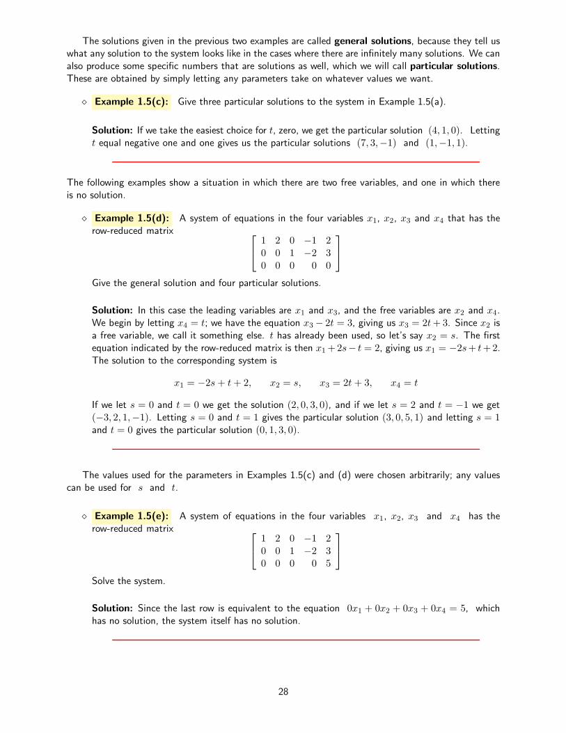
The solutions given in the previous two examples are called general solutions, because they tell uswhat any solution to the system looks like in the cases where there are infinitely many solutions. We canalso produce some specific numbers that are solutions as well, which we will call particular solutions.These are obtained by simply letting any parameters take on whatever values we want.
⋄ Example 1.5(c): Give three particular solutions to the system in Example 1.5(a).
Solution: If we take the easiest choice for t, zero, we get the particular solution (4, 1, 0). Lettingt equal negative one and one gives us the particular solutions (7, 3,−1) and (1,−1, 1).
The following examples show a situation in which there are two free variables, and one in which thereis no solution.
⋄ Example 1.5(d): A system of equations in the four variables x1, x2, x3 and x4 that has therow-reduced matrix
1 2 0 −1 20 0 1 −2 30 0 0 0 0
Give the general solution and four particular solutions.
Solution: In this case the leading variables are x1 and x3, and the free variables are x2 and x4.We begin by letting x4 = t; we have the equation x3− 2t = 3, giving us x3 = 2t+3. Since x2 isa free variable, we call it something else. t has already been used, so let’s say x2 = s. The firstequation indicated by the row-reduced matrix is then x1+2s− t = 2, giving us x1 = −2s+ t+2.The solution to the corresponding system is
x1 = −2s+ t+ 2, x2 = s, x3 = 2t+ 3, x4 = t
If we let s = 0 and t = 0 we get the solution (2, 0, 3, 0), and if we let s = 2 and t = −1 we get(−3, 2, 1,−1). Letting s = 0 and t = 1 gives the particular solution (3, 0, 5, 1) and letting s = 1and t = 0 gives the particular solution (0, 1, 3, 0).
The values used for the parameters in Examples 1.5(c) and (d) were chosen arbitrarily; any valuescan be used for s and t.
⋄ Example 1.5(e): A system of equations in the four variables x1, x2, x3 and x4 has therow-reduced matrix
1 2 0 −1 20 0 1 −2 30 0 0 0 5
Solve the system.
Solution: Since the last row is equivalent to the equation 0x1 + 0x2 + 0x3 + 0x4 = 5, whichhas no solution, the system itself has no solution.
28

Section 1.5 Exercises To Solutions
1. Consider the system of equations
2x− 4y − z = −44x− 8y − z = −4−3x+ 6y + z = 4
.
(a) Determine which of the following ordered triples are solutions to the system of equations:
(6, 3, 4) (3,−1, 4) (0, 0, 4) (−2,−1, 4) (5, 2, 0) (2, 1, 4)
Look for a pattern in the ordered triples that ARE solutions. Try to guess another solution,and test your guess by checking it in all three equations. How did you do?
(b) When you tried to solve the system using your calculator, you should have gotten the reducedechelon matrix as
1 −2 0 00 0 1 40 0 0 0
.
Give the system of equations that this matrix represents. Which variable can you determine?
(c) It is not possible to determine y, so we simply let it equal some arbitrary value, which wewill call t. So at this point, z = 4 and y = t. Substitute these into the first equationand solve for x. Your answer will be in terms of t. Write the ordered triple solution to thesystem.
NOTE: The system of equations you obtained in part (b) and solved in part (c) has infinitelymany solutions, but we do know that every one of them has the form (2t, t, 4). Note how thisexplains the results of part (a).
2. The reduced echelon form of the matrix for the system
3x− 2y + z = −72x+ y − 4z = 0
x+ y − 3z = 1
is
1 0 −1 −10 1 −2 20 0 0 0
.
(a) Give the free variable(s) and leading variable(s).
(b) In this case, z cannot be determined, so we let z = t. Now solve for y, in terms of t. Thensolve for x in terms of t.
(c) Pick a specific value for t and substitute it into your general form of a solution triple for thesystem. Check it by substituting it into all three equations in the original system.
(d) Repeat (b) for a different value of t.
29

3. The reduced echelon forms of some systems are given below.
• If the system has a unique solution, give it. If the system has no solution, say so.
• If the system has infinitely many solutions, give the general solution in terms of parameterss, t, etc., then give two particular solutions.
(a)
1 0 −1 0 40 1 2 0 −50 0 0 1 3
(b)
1 3 0 0 50 0 1 0 10 0 0 1 −4
(c)
1 −3 0 1 −40 0 1 −2 50 0 0 0 0
(d)
1 0 1 50 1 2 −30 0 0 1
(e)
1 0 −2 1 60 1 3 5 −30 0 0 0 0
(f)
1 0 0 −10 1 0 20 0 1 0
(g)
1 2 −1 10 0 0 00 0 0 0
(h)
1 4 −1 0 −20 0 0 1 70 0 0 0 1
(i)
1 5 0 0 20 0 1 0 10 0 0 1 −40 0 0 0 0
4. Give four particular solutions from the general solution of Example 1.5(b), which had generalsolution (−3t− 1, 5t + 2, t, 4).
5. For the systems whose augmented matrices row reduce to the forms shown below, do one of thefollowing:
• If the system has a unique solution, give it. If the system has no solution, say so.
• If the system has infinitely many solutions, give the general solution in terms of parameterss, t, etc., then give two particular solutions.
1 1 −10 0 20 0 0
1 2 −1 0 50 0 0 1 −40 0 0 0 0
30

1.6 Back to Applications
Performance Criterion:
1. (l) Use systems of equations to solve network problems.
The concept of a network was introduced in Exercise 7 of Section 1.1. To review, a network is aset of junctions, which we’ll call nodes, connected by what could be called pipes, or wires, but whichwe’ll call directed edges. The word “directed” is used to mean that we’ll assign a direction of flow toeach edge. There will also be directed edges coming into or leaving the network. It is probably easiestto just think of a network of plumbing, with water coming in at perhaps several places, and leaving atseveral others.
Our study of networks will be based on one simple idea, known as conservation of flow:
At each node of a network, the flow into the node must equal the flow out.
⋄ Example 1.6(a): A one-node network is shown to the right. Find theunknown flow f .
Solution: The flow in is 20 + f and the flow out is 45 + 30, so wehave
20 + f = 45 + 30.
Solving, we find that f = 55.
f
3045
20
⋄ Example 1.6(b): Another one-node network is shown to the right.Find the unknown flow f .
Solution: The flow in is 70 + f and the flow out is 15 + 30, so wehave
70 + f = 15 + 30.
Solving, we find that f = −25, so the flow at the arrow labeled f isactually in the direction opposite to the arrow.
f
3015
70
When setting up a network we must commit to a direction of flow for any edges in which the flow isunknown, but when solving the system we may find that the flow is in the opposite direction from theway the edge was directed initially, as we just saw. We may also have less information than we did inthe previous two examples, as shown by the next example.
31

⋄ Example 1.6(c): For the one-node network is shown to the right, findthe unknown flow f1 in terms of the flow f2.
Solution: By conservation of flow,
50 + f2 = f1 + 35.
Solving for f1 gives us f1 = f2+15. Thus if f2 was 10, f1 wouldbe 25 (look at the diagram and think about that), if f2 was 45,f1 would be 60, and so on.
f2
35f1
50
The previous example represents, in an applied setting, the idea of a free variable. In this exampleeither variable can be taken as free, but if we know the value of one of them, we’ll “automatically” knowthe value of the other. The way the example was worded, we were taking f2 to be the free variable,with the value of f1 then depending on the value of f2.
The systems in these first three examples have been very simple; let’s now look at a more complexsystem.
⋄ Example 1.6(d): Determine the flows f1, f2, f3 and f4 inthe network shown to the right.
Solution: Utilizing conservation of flow at each node, we getthe equations
30 + 15 = f1 + f2, 70 + f2 = f3,
f1 = 40 + f4, f3 + f4 = 20 + 55
Rearranging these give us the system of equations shown belowand to the left. The augmented matrix for this system reducesto the matrix shown below and to the right.
f1
f2f3
f4
3015
70
40
55
20
f1 + f2 = 45f2 − f3 = −70
f1 − f4 = 40f3 + f4 = 75
=⇒
1 1 0 0 450 1 −1 0 −701 0 0 −1 400 0 1 1 75
=⇒
1 0 0 −1 400 1 0 1 50 0 1 1 750 0 0 0 0
From this we can see that f4 is a free variable, so lets say it has value t. The solution to thenetwork is then
f1 = 40 + t, f2 = 5− t, f3 = 75 − t, f4 = t,
where t is the flow f4.
Underdetermined and Overdetermined Systems
Let’s think a bit more about this last example. Suppose that f4 = t = 0. The equations given asthe solution to the network then give us f1 = 40, f2 = 5, f3 = 75. We can see this without evensolving the system of equations. Looking at the node in the lower right, if f4 = 0 one can easily see
32

that f3 must be 75 in order for the flow in to equal the flow out. Knowing f3, we can go to thenode in the lower left and see that f2 = 5. Finally, f2 = 5 gives is f1 = 40. The informationgiven originally was not sufficient to determine the values of the flows f1, f2, f3 and f4. In such acase, we sometimes say that the system is undetermined, meaning that there is too little informationto guarantee a single solution. We just saw that with one more piece of information, the value of f4,all of the remaining flows were then determined by that value.
Now consider the situation described in Exercise 6 of Section 1.1. Given the points
(1.2, 3.7) (2.5, 4.1) (3.2, 4.7) (4.3, 5.2) (5.1, 5.9)
we wish to find the equation y = mx + b of a line containing them. Substituting each pair intoy = mx+ b gives us the system shown below and to the left.
1.2m + b = 3.72.5m + b = 4.13.2m + b = 4.74.3m + b = 5.25.1m + b = 5.9
=⇒
1.2 1 3.72.5 1 4.13.2 1 4.74.3 1 5.25.1 1 5.9
rref=⇒
1 0 00 1 00 0 10 0 00 0 0
4
4x
y
When we row-reduce the augmented matrix for this system, we get the last matrix above, indicatingthat the system has no solution. The five points are plotted above and to the right, and we can seethat they are not on a line, which is why we were not able to solve the system. In this case the systemis overdetermined, meaning that there is too much information to allow a solution to the system.
You might think “Well, why not just use less data, so that the resulting system has a solution?”Well the additional data gives us some redundancy that can give us better results if we know how todeal with it. The way out of this problem is a method called least-squares, which we’ll see later. It isa method for dealing with systems that don’t have solutions. What it allows us to do is obtain valuesthat are in some sense the “closest” values there are to an actual solution. Again, more on this later.
Section 1.6 Exercises To Solutions
f1f2
f3 f4
8
18
f5
f6
1. The network to the right represents a traffic circle. The numbersnext to each of the paths leading into or out of the circle are thenet flows in the directions of the arrows, in vehicles per minute,during the first part of lunch hour.
(a) Suppose that f3 = 7 and f5 = 4. You should be ableto work your way around the circle, eventually figuring outwhat each flow is. Do this.
(b) Now assume that the only flows you know are the ones shown in the diagram. When youset up a system of equations, based on the flows in and out of each junction, how manyequations will you have? How many unknowns?
(c) Go ahead and set up the system of equations. Give the augmented matrix and the reducedmatrix (obtained with your calculator), and then give the general solution to the system.
(d) Choose the value(s) of the parameter(s) that make f3 = 7 and f5 = 4, then find theresulting particular solution. If your answers do not match what you got for part (a), goback and check your work for (c).
(e) What restriction(s) is(are) there on the parameter(s), in order that all flows go in the direc-tions indicated. (Allow a flow of zero for each flow as well.)
33

2. For another traffic circle, a student uses the diagram shown to theright and obtains the flows given below, in vehicles per minute.
f1 = t− 8, f2 = t+ 3, f3 = t− 5, f4 = t
(a) Determine the minimum value of t that makes each off1 through f4 zero or greater. Give the minimum allow-able values for each flow, in the form fi ≥ a, assuming thatno vehicles ever go the wrong way around a portion of the cir-cle. Remember that setting a value for any flow determines allthe other flows. You may neglect units.
f1f2
f3 f4
fa
fb
fc
fd
(b) Give each of the flows f1 through f4 when the flow in the northeast quarter (f1) is 12vehicles per minute. You may neglect units.
(c) Determine each of the flows fa through fd, still for f1 = 12. You should be able to dothis based only on the four equations given. At least one of them will be negative, indicatingthat the corresponding arrow(s) should be reversed.
34

1.7 Chapter 1 Exercises
1. Consider the system of equations below and to the right. Solvethe system by Gaussian elimination (get in row-echelon form,then perform back substitution), by hand (no calculator). Showall steps, including what operation was performed for each step.Hint: You may find it useful to put the equations in a differentorder before forming the augmented matrix.
5x− y + 2z = 17
x+ 3y − z = −42x+ 4y − 3z = −9
2. Find the equation of the parabola through the points (0, 3), (1, 4) and (3, 18).
3. Consider the points (1, 5), (2, 2), (4, 3) and (5, 4).
(a) What is the smallest degree polynomial whose graph will contain all of these points?
(b) Find the polynomial whose graph contains all the points.
(c) Check by graphing on your calculator.
4. Why would we not be able to find the equation of a line through (0, 6), (2, 3) and (6, 1)? We willsee later what this means in terms of systems of equations, and we will resolve the problem in areasonable way.
5. Find the equation of the plane through the three points P1(4, 1,−3), P2(0,−5, 1) and P3(3, 3, 2).
6. (a) A student is attempting to find the equilibrium temperatures at points t1, t2, t3 andt4 on a plate with a grid and boundary temperatures shown below and to the left. They gett1 = 50.3, t2 = 67.4, t3 = 53.6, t4 = 60.5. Explain in one complete sentence why theiranswer must be incorrect, without finding the solution.
t1 t2
t3 t4
47
51
66
62
52 58
55 57
4 −1 0 0 −1 0 103
−1 4 −1 0 0 −1 92
0 −1 4 −1 −1 0 110
0 0 −1 4 0 0 98
−1 0 −1 0 4 0 105
0 −1 0 0 −1 4 107
(b) A different student is trying to solve another such problem, and their augmented matrix isshown above and to the right. How do we know that one of their equations is incorrect,without setting up the equations ourselves?
7. Suppose we are solving a system of three equations in the three unknowns x1, x2 and x3, withthe unknowns showing up in the equations in that order. It is possible to do row reduction in sucha way as to obtain the matrix
1 0 0 53 −2 0 7−1 5 2 −3
Determine x1, x2 and x3 without row-reducing this matrix! you should be able to simply setup equations and find values for the unknowns.
35

8. Given a cube of some solid material, it is possible to puta three-dimensional grid into the solid, in the same waythat we put a two-dimensional grid on a rectangular plate.Given temperatures at all nodes on the exterior faces of thecube, we can find equilibrium temperatures at each interiornode using a system of equations. Once again the key isthe mean-value property. In this three dimensional case thisproperty tells us that the equilibrium temperature at eachinterior node is equal to the average of all the temperaturesat nodes of the grid that are immediately adjacent to thepoint in question. To the right I have shown a cube thathas eight interior grid points. The word “slice” is used hereto mean a cross section through
front face slice 1slice 2
back face (behind)
the cube. The grids below show temperatures, known or unknown, at all nodes on the front face,each of the two slices, and the back face. Above and to the right I have “exploded” the cube toshow the temperatures on the front and back faces, and the two slices. Of course each node onany slice is connected to the corresponding node on the adjacent slice or face.
37 40
39 41
front face
t11 t12
t13 t14
41 42
40 41
40 43
40 44
slice 1
t21 t22
t23 t24
45 48
43 45
43 50
42 49
slice 2
47 54
49 52
back face
(a) Using the Mean Value Property in three dimensions, the temperature at each interior pointwill NOT be the average of four temperatures, like it was on a plate. How many temperatureswill be averaged in this case?
(b) Set up a system of equations to solve for the interior temperatures, and find each to thenearest tenth.
9. Do any of your observations from Exercise 7 change in the three dimensional case?
10. Do one of the following for each of the systems whose augmented matrices row reduce to theforms shown below. Assume that the unknowns are x1, x2, ...
• If the system has a unique solution, give it. If the system has no solution, say so.
• If the system has infinitely many solutions, give the general solution in terms of parameterss, t, etc., then give two particular solutions.
(a)
1 0 −10 1 00 0 0
(b)
1 0 −1 0 −40 1 2 0 50 0 0 1 2
(c)
1 1 −10 0 20 0 0
36

11. Consider the row-echelon augmented matrix
1 −1 3 −2 4
0 0 1 2 −50 0 0 2 −80 0 0 0 0
.
(a) Give the general solution to the system of equations that this arose from.
(b) Give three specific solutions to the system.
(c) Change one entry in the matrix so that the system of equations would have no solution.
12. Vail, Colorado recently put in traffic “round-a-bouts” at all of its exits off Interstate 70. Eachof these consists of a circle in which traffic is only allowed to flow counter-clockwise (do thatall turns are right turns), and four points at which the circle can be entered or exited. See thediagram below.
town
frontage road
I-70 EastI-70 West
N⇑
It is known that at 7:30 AM the following is occurring:
• 22 vehicles per minute are entering the roundabout from the west. (These are the workerswho cannot afford to live in Vail, and commute on I-70 from towns 30 and 40 miles west.)
• 4 vehicles per minute are exiting the roundabout to go east on I-70. (These are the touristsheaded to the airport in Denver.)
• 7 vehicles per minute are exiting the roundabout toward town and 11 per minute are exitingtoward the frontage road.
Solve the system and answer the following:
(a) What is the minimum number of cars per minute passing through the southeast quarter ofthe roundabout?
(b) If 18 vehicles per minute are passing through the southeast (SE) quarter of the roundaboutper minute, how many are passing through each of the other quarters (NW, NE, SW)?
13. Consider the system
x1 − x2 − 4x3 = 6
5x1 + x2 − 2x3 = 18
2x1 + 4x2 + 10x3 = 0
.
(a) Use your calculator or an online tool to reduce the matrix to reduced row echelon form.Write the system of two equations represented by the first two rows of the reduced matrix.(The last equation is of no use, so don’t bother writing it.)
37

(b) The second equation contains x2 and x3. Suppose that x3 = 1 and compute x2 usingthat equation. Then use the values you have for x2 and x3 in the first equation to findx1.
(c) Verify that the values you obtained in (b) are in fact a solution to the original system given.
(d) Now let x3 = 0 and repeat the process from (b) to obtain another solution. Verify thatsolution as well.
(e) Let x3 = 2 to find yet another solution.
(f) Because there is no equation allowing us to determine x3, we say that it is a free variable.What we will usually do in situations like this is let x3 equal some parameter (number) thatwe will denote by t. That is, we set x3 = t, which is really just renaming it. Substitutet into the second equation from (a) and solve for x2 in terms of t. Then substitute thatresult into the first equation for x2, along with t for x3, and solve for x1 in terms oft. Summarize by giving each of x1, x2 and x3 in terms of t, all in one place.
(g) Substitute the number one for t into your answer to (f) and check to see that it matcheswhat you got for (b). If doesn’t, you’ve gone wrong somewhere - find the error and fix it.
14. Solve each of the following systems of equations that have solutions. Do/show the followingthings:
• Enter the augmented matrix for the system in your calculator.
• Get the row-reduced echelon form of the matrix using the rref command. Write down theresulting matrix.
• Write the system of equations that is equivalent to the row-reduced echelon matrix.
• Find the solutions, if there are any. Use the letters that were used in the original system forthe unknowns! For those with multiple solutions, give them in terms of a parameter t or,when necessary, two parameters s and t.
(a)
x1 − x2 + 3x3 = −4−2x1 + 3x2 − 8x3 = 13
5x1 − 3x2 + 11x3 = −10(b)
c1 + 3c2 + 5c3 = 3
2c1 + 7c2 + 9c3 = 5
2c1 + 6c2 + 11c3 = 7
(c)
x1 + 3x2 − 2x3 = −1−7x1 − 21x2 + 14x3 = 7
2x1 + 6x2 − 4x3 = −2(d)
c1 − c2 + 3c3 = −4−2c1 + 3c2 − 8c3 = 13
5c1 − 3c2 + 11c3 = 4
(e)
x− 3y + 7z = 4
5x− 14y + 42z = 29
−2x+ 5y − 20z = −16(f)
x+ 3y = 2
4x+ 12y + z = 1
−x− 3y − 2z = 12
• Give three specific solutions to the system from part (a) above.
• Give three specific solutions to the system from part (c) above.
• Solve the system from part (b) above by hand, showing all steps of the row reduction andindicating what you did at each step.
38

15. Give the reduced row echelon form of an augmented matrix for a system of four equations in fourunknowns x1, x2, x3 and x4 for which
• x4 = 7
• x2 and only x2, is a free variable
16. (Erdman) Consider the systemx+ ky = 1kx+ y = 1
, where k is some constant.
(a) Set up the augmented matrix and use a row operation to get a zero in the lower left corner.
(b) For what value or values of k would the system have infinitely many solutions? What isthe form of the general solution?
(c) For what value or values of k would the system have no solution?
(d) For all remaining values of k the system has a unique solution (that depends on the choiceof k). What is the solution in that case? Your answer will contain the parameter k.
17. (Erdman) Consider the systemx− y − 3z = 3
2x+ z = 02y + 7z = c
, where c is some constant.
(a) Set up the augmented matrix and use a row operation to get a zero in the first entry of thesecond row.
(b) Look at the second and third rows. For what value or values of c can the system be solved?Give the solution if there is a unique solution. Give the general solution if there are infinitelymany solutions.
18. In a previous exercise, you may have attempted to find the equation of a parabola through thethree points (−1,−6), (0,−4) and (1,−1). You set up a system to find values of a, b and c inthe parabola equation y = ax2 + bx+ c. There was a unique solution, meaning that there is onlyone parabola containing those three points. Expect the following to not work out as “neatly.”
(a) Use a system of equations to find the equation of a parabola that goes through just the twopoints (−1,−6) and (1,−1). Explain your results.
(b) Use a system of equations to find the equation y = mx+ b of a line through the four points(1.3, 1.5), (0.8, 0.4), (2.6, 3.0) and (2.0, 2.0).
(c) Plot the four points from (b) on a neat and accurate graph, and use what you see to explainyour answer to (b). You should be able to give your explanation in one or two completesentences.
39
2 Euclidean Space and Vectors
Outcome:
2. Understand vectors and their algebra and geometry in Rn. Understand the
relationship of vectors to systems of equations.
Performance Criteria:
(a) Recognize the equation of a plane in R3 and determine where the plane
intersects each of the three axes. Sketch a graph of the part of a planein the first quadrant. Give the equation of a plane from a geometricdescription.
(b) Find the vector from one point to another in Rn. Find the length of a
vector in Rn.
(c) Multiply vectors by scalars and add vectors, algebraically. Find linearcombinations of vectors algebraically.
(d) Illustrate the parallelogram method and tip-to-tail method for finding alinear combination of two vectors.
(e) Find a linear combination of vectors equalling a given vector.
(f) Give the linear combination form of a system of equations, give thesystem of linear equations equivalent to a given vector equation.
(g) Sketch a picture illustrating the linear combination form of a system ofequations of two equations in two unknowns.
(h) Give an algebraic description of a set of a set of vectors that has beendescribed geometrically, and vice-versa.
(i) Determine whether a set of vectors is closed under vector addition; de-termine whether a set of vectors is closed under scalar multiplication. Ifit is, prove that it is; if it is not, give a counterexample.
(j) Give the vector equation of a line through two points in R2 or R
3 orthe vector equation of a plane through three points in R
3.
(k) Write the solution to a system of equations in vector form and determinethe geometric nature of the solution.
In the study of linear algebra we will be defining new concepts and developing corresponding notation.The purpose of doing so is to develop more powerful machinery for investigating the concepts of interest.We begin the development of notation with the following. The set of all real numbers is denoted byR, and the set of all ordered pairs of real numbers is R
2, spoken as “R-two.” Geometrically, R2 is
the familiar Cartesian coordinate plane. Similarly, the set of all ordered triples of real numbers is thethree-dimensional space referred to as R
3, “R-three.” The set of all ordered n-tuples (lists of n realnumbers in a particular order) is denoted by R
n. Although difficult or impossible to visualize physically,Rn can be thought of as n-dimensional space. All of the R
ns are what are called Euclidean space.
40

2.1 Euclidean Space
Performance Criteria:
2. (a) Recognize the equation of a plane in R3 and determine where the plane
intersects each of the three axes. Sketch a graph of the part of a planein the first quadrant. Give the equation of a plane from a geometricdescription.
It is often taken for granted that everyone knows what we mean by the real numbers. To actuallydefine the real numbers precisely is a bit of a chore and very technical. Suffice it to say that the realnumbers include all numbers other than complex numbers (numbers containing
√−1 = i or, for
electrical engineers, j) that a scientist or engineer is likely to run into. The numbers 5, −31.2, π,√2, 2
7 , and e are all real numbers. We denote the set of all real numbers with the symbol R, andthe geometric representation of the real numbers is the familiar real number line, a horizontal line onwhich every real number has a place. This is possible because the real numbers are ordered: given anytwo real numbers, either they are equal to each other, one is less than the other, or vice-versa.
As mentioned previously, the set R2 is the set of all ordered pairs of real numbers. Geometrically,
every such pair corresponds to a point in the Cartesian plane, which is the familiar xy-plane. R3 is
the set of all ordered triples, each of which represents a point in three-dimensional space. We cancontinue on - R
4 is the set of all ordered “4-tuples”, and can be thought of geometrically as fourdimensional space. Continuing further, an “n-tuple” is n real numbers, in a specific order; each n-tuplecan be thought of as representing a point in n-dimensional space. These spaces are sometimes called“two-space,” “three-space” and “n-space” for short.
Two-space is fairly simple, with the only major features being the two axes and the four quadrantsthat the axes divide the space into. Three-space is a bit more complicated. Obviously there are threecoordinate axes instead of two. In addition to those axes, there are also three coordinate planes as well,the xy-plane, the xz-plane and the yz-plane. Finally the three coordinate planes divide the space intoeight octants. The pictures below illustrate the coordinate axes and planes. The first octant is theone we are looking into, where all three coordinates are positive. It is not important that we know thenumbering of the other octants.
x
y
z
origin
positivex-axis
negativex-axis
x
y
z
xy-plane
yz-plane
xz-plane
Every plane in R3 (we will be discussing only R
3 for now) consists of a set of points that behavein an orderly mathematical manner, described here:
41

Equation of a Plane in R3: The ordered triples corresponding to all the points in
a plane satisfy an equation of the form
ax+ by + cz = d, (1)
where a, b, c and d are constants, and not all of a, b and c are zero.
Note that equation (1) is a linear equation! The equation of any line in R2 can be written in the
form ax+ by = c, which is also a linear equation. A line is a one-dimensional object and a plane is atwo-dimensional object, in a sense that we will see later. ax+ by = c then describes a one-dimensional“straight” object in the two-dimensional space R
2, and (1) describes a two-dimensional “flat” objectin R
3. The corresponding equation in Rn is
a1x1 + a2x2 + a3x3 + · · ·+ anxn = b, (2)
where all of a1, a2, ..., an and b are numbers and x1, x2, ..., xn are unknowns. (2) describesan n − 1-dimensional object in n-dimensional space. When n > 3 we often call such an object ahyperplane.
Going back to (1) as describing a plane in R3, the xy-plane in R
3 is the plane containing thex and y-axes. The only condition on points in that plane is that z = 0, so that is the equation ofthat plane. In that case the constants a, b and d are all zero, and c = 1. The plane z = 5 is ahorizontal plane that is five units above the xy-plane, and x = −2 describes the vertical plane thatis parallel to the yz-plane and passes through the x-axis at x = −2. What about an equation of theform ax+ by = c when we are in R
3?
⋄ Example 2.1(a): Graph the equation 2x+ 3y = 6 in the first octant. Indicate clearly whereit intersects each of the coordinate axes, if it does.
Solution: Some points that satisfy the equation are (3, 0, 0),(6,−2, 5), and so on. Since z is not included in the equation,there are no restrictions on z; it can take any value. If we wereto fix z at zero and plot all points that satisfy the equation, wewould get a line in the xy-plane through the two points (3, 0, 0)and (0, 2, 0). These points are obtained by first letting y andz be zero, then by letting x and z be zero. Since z can beanything, the set of points satisfying 2x+ 3y = 6 is a verticalplane intersecting the xy-plane in that line. The plane is shownto the right.
x
y
z
3
2
Next we’ll see how we can sometimes graphically represent a portion of a plane in 3-space.
42

⋄ Example 2.1(b): Graph the equation 2x + 3y + z = 6 in the first octant. Indicate clearlywhere it intersects each of the coordinate axes, if it does.
Solution: The set of points satisfying this equation is also aplane, but z is no longer free to take any value. The simplest wayto “get a handle on” such a plane is to find where it interceptsthe three axes. Note that every point on the x-axis has y- andz-coordinates of zero. So to find where the plane intersects thex-axis we put zero into the equation for y and z, then solvefor x, getting x = 3. The plane then intersects the x-axis at(3, 0, 0). A similar process gives us that the plane intersects they and z axes at (0, 2, 0) and (0, 0, 6). From this informationwe get that the graph of the plane is that shown in the drawingabove and to the right.
x
y
z
6
3
2
Consider now a system of equations like
x+ 3y − 2z = −43x+ 7y + z = 4
−2x+ y + 7z = 7
,
which has solution (3,−1, 2). We now know that each of the three equations represents a plane inR3. The point (3,−1, 2) is where the three planes intersect! This is completely analogous to the
interpretation of the solution of a system of two linear equations in two unknowns as the point wherethe two lines representing the equations cross. This is the first of three interpretations we’ll have forthe solution to a system of equations.
The only other basic geometric fact we need about three-space is this:
Distance Between Points: The distance between two points (x1, y1, z1) and(x2, y2, z2) in R
3 is given by
d =√
(x1 − x2)2 + (y1 − y2)2 + (z1 − z2)2
This is simply a three-dimensional version of the Pythagorean Theorem, and an equivalent formula isused in higher dimensions. Even though we cannot visualize the distance geometrically, this idea is bothmathematically valid and useful in applications.
⋄ Example 2.1(c): Find the distance in R4 between the points (−4, 7, 1,−5) and (13, 0,−6, 2).
Solution: Using the above formula with one more dimension we get
d =√
(−4− 13)2 + (7− 0)2 + (1− (−6))2 + (−5− 2)2
=√
(−17)2 + 72 + 72 + (−7)2 =√436 ≈ 20.9
43

Section 2.1 Exercises To Solutions
1. Determine whether each of the equations given describes a plane in R3. If not, say so. If it does
describe a plane, give the points where it intersects each axis. If it doesn’t intersect an axis, sayso.
(a) −2x− y + 3z = −6 (b) x+ 3z = 6 (c) y = −6(d) x+ 3z2 = 12 (e) x− 2y + 3z = −6
2. (a) Give an equation of the plane in R3 that intersects the x-axis at 2, the y-axis at 5, and
the z-axis at 4.
(b) Give an equation of the plane in R3 that intersects the x-axis at −3, the y-axis at 1,
and the z-axis at 7.
(c) Give an equation of the plane in R3 that intersects the x-axis at 3, the z-axis at −2,
and does not intersect the y-axis.
(d) Give an equation of the plane in R3 that intersects the y-axis at 4 and does not intersect
either of the other two axes.
(e) Give an equation of the plane in R3 that intersects the y-axis at −4, the z-axis at 1,
and does not intersect the x-axis.
(f) Give an equation of the plane in R3 that intersects the z-axis at −2 and does not intersect
either of the other two axes.
3. Each of the following equations describes a plane in R3. For
each, sketch the graph of the part of the plane in the first octant,in the manner done in Examples 2.1(a) and (b). Begin with asketch of the positive parts of the three coordinate axes, asshown to the right.
x
y
z
(a) 2x+ 2y + 5z = 10 (b) 2y + 3z = 6
(c) x+ 3y = 6 (d) 2x+ 4y + z = 8
(e) z = 3 (f) 3x+ y + 2z = 6
(g) 2x+ 4z = 8 (h) y = 5 (i) 3x+ y + 3z = 3
44

2.2 Introduction to Vectors
Performance Criteria:
2. (b) Find the vector from one point to another in Rn. Find the length of a
vector in Rn.
There are a number of different ways of thinking about vectors; it is likely that you think of themas “arrows” in two- or three-dimensional space, which is the first concept of a vector that most peoplehave. Each such arrow has a length (sometimes called norm or magnitude) and a direction. Physically,then, vectors represent quantities having both amount and direction. Examples would be things likeforce or velocity. Quantities having only amount, like temperature or pressure, are referred to as scalarquantities. We will represent scalar quantities with lower case italicized letters like a, b, c, ..., x, y, z andwe’ll represent vectors with lower case boldface letters with “harpoon” arrows over them, like
u,
v,
x,and so on.. In many texts vectors are denoted just by lower case boldface letters like u, v, x, and soon. When writing by hand we’ll just put a small arrow (harpoon or regular) pointing to the right overany letter denoting a vector, without trying to make the letter boldface.
Consider a vector represented by an arrow in R2. We will call
the end with the arrowhead the tip of the vector, and the other endwe’ll call the tail. (The more formal terminology is terminal pointand initial point.) The picture to the right shows three vectors
u,
v and
w in R2. It should be clear that a vector can be moved
around in R2 in such a way that the direction and magnitude
remain unchanged. Sometimes we say that two vectors related toeach other this way are equivalent, but in this class we will simplysay that they are the same vector. The vectors
u and
v are thesame vector, just in different positions.
5
5
u
v
w
P
Q
R
x
y
It is sometimes convenient to denote points with letters, and we use italicized capital letters forthis. We commonly use P (for point!) Q and R, and the origin is denoted by O. (That’s capital“oh,” not zero.) Sometimes we follow the point immediately by its coordinates, like P (−4, 2). The
notation−−→PQ denotes the vector that goes from point P to point Q, which in this case is vector
u.
Any vector−−→OR with its tail at the origin is said to be in standard position, and is called a position
vector;
w above is an example of such a vector. Note that for any point in R2 (or in R
n), thereis a corresponding vector that goes from the origin to that point. In linear algebra we think of a pointand its position vector as interchangeable. In the next section you will see the advantage of thinking ofa point as a position vector.
We will describe vectors with numbers - in R2 we give a vector as two numbers, the first telling
how far to the right (positive) or left (negative) one must go to get from the tail to the tip of the vector,and the second telling how far up (positive) or down (negative) from tail to tip. These numbers aregenerally arranged in one of two ways. The first way is like an ordered pair, but with “square brackets”instead of parentheses. The vector
u above is then
u = [7, 3], and
w = [2,−4]. The second
way to write a vector is as a column vector:
u =
[
73
]
. This is, in fact, the form we will use more
often. Observe that the vector from one point to another is obtained by subtracting the corresponding
coordinates of the first point from those of the second point. So the vector−−→PQ from P (−4, 2) to
Q(3, 5) is−−→PQ =
[
3− (−4)5− 2
]
=
[
73
]
.
45
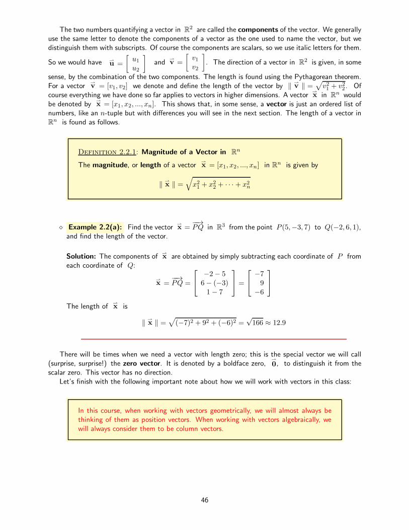
The two numbers quantifying a vector in R2 are called the components of the vector. We generally
use the same letter to denote the components of a vector as the one used to name the vector, but wedistinguish them with subscripts. Of course the components are scalars, so we use italic letters for them.
So we would have
u =
[
u1u2
]
and
v =
[
v1v2
]
. The direction of a vector in R2 is given, in some
sense, by the combination of the two components. The length is found using the Pythagorean theorem.For a vector
v = [v1, v2] we denote and define the length of the vector by ‖
v ‖ =√
v21 + v22 . Ofcourse everything we have done so far applies to vectors in higher dimensions. A vector
x in Rn would
be denoted by
x = [x1, x2, ..., xn]. This shows that, in some sense, a vector is just an ordered list ofnumbers, like an n-tuple but with differences you will see in the next section. The length of a vector inRn is found as follows.
Definition 2.2.1: Magnitude of a Vector in Rn
The magnitude, or length of a vector
x = [x1, x2, ..., xn] in Rn is given by
‖
x ‖ =√
x21 + x22 + · · ·+ x2n
⋄ Example 2.2(a): Find the vector
x =−−→PQ in R
3 from the point P (5,−3, 7) to Q(−2, 6, 1),and find the length of the vector.
Solution: The components of
x are obtained by simply subtracting each coordinate of P fromeach coordinate of Q:
x =−−→PQ =
−2− 56− (−3)1− 7
=
−79−6
The length of
x is
‖
x ‖ =√
(−7)2 + 92 + (−6)2 =√166 ≈ 12.9
There will be times when we need a vector with length zero; this is the special vector we will call(surprise, surprise!) the zero vector. It is denoted by a boldface zero,
0, to distinguish it from thescalar zero. This vector has no direction.
Let’s finish with the following important note about how we will work with vectors in this class:
In this course, when working with vectors geometrically, we will almost always bethinking of them as position vectors. When working with vectors algebraically, wewill always consider them to be column vectors.
46

Section 2.2 Exercises To Solutions
1. Find the magnitude of each vector - label each answer using correct notation.
u =
−312
,
x =
[
−57
]
,
v =
1234
,
b =
b1b2b3b4
2. For each pair of points P and Q, find the vector−−→PQ in the appropriate space. Then find the
length of the vector.
(a) P (−4, 11, 7), Q(13, 5,−8) (b) P (−5, 1), Q(7,−2)(c) P (−3, 0, 6, 1), Q(7,−1,−1, 10)
3. (a) The vector−−→PQ =
[
2−1
]
in R2 has initial point P (3, 5). What is the terminal point
Q?
(b) The vector−−→PQ = [4, 0,−2, 1, 5] in R
5 has initial point P (−2, 7, 1,−8, 2). What is theterminal point Q?
(c) The vector−−→PQ =
−46−1
in R3 has terminal point Q(5,−2, 4). What is the initial
point P?
4. Consider the vector
u =
21−2
in R3.
(a) Find the magnitude ‖
u ‖, labeling it as such.
(b) Later we will define what we mean by multiplication or division of a vector by a scalar. Divide
each component of
u by your answer to (a). The result is the vector
u
‖
u ‖, so label it
that way.
(c) Find
∥
∥
∥
∥
u
‖
u ‖
∥
∥
∥
∥
, the magnitude of
u
‖
u ‖from (b).
5. Repeat Exercise 4 for the vector
v =
[
4−3
]
in R2. How does your final result compare with
that of Exercise 4?
47

2.3 Addition and Scalar Multiplication of Vectors, Linear Combinations
Performance Criteria:
2. (c) Multiply vectors by scalars and add vectors, algebraically. Find linearcombinations of vectors algebraically.
(d) Illustrate the parallelogram method and tip-to-tail method for finding alinear combination of two vectors.
(e) Find a linear combination of vectors equalling a given vector.
In the previous section a vector
x = [x1, x2, ..., xn] in n dimensions was starting to looksuspiciously like an n-tuple (x1, x2, ..., xn) and we established a correspondence between any pointand the position vector with its tip at that point. One might wonder why we bother then with vectorsat all! The reason is that we can perform algebraic operations with vectors that make sense physically,while such operations make no sense with n-tuples. The two most basic things we can do with vectorsare add two of them or multiply one by a scalar, and both are done component-wise:
Definition 2.3.1: Addition and Scalar Multiplication of Vectors
Let
u = [u1, u2, ..., un] and
v = [v1, v2, ..., nn], and let c be a scalar. Then wedefine the vectors
u +
v and c
u by
u +
v =
u1u2...un
+
v1v2...vn
=
u1 + v1u2 + v2
...un + vn
and c
u = c
u1u2...un
=
cu1cu2...
cun
Note that result of adding two vectors or multiplying a vector by a scalar is also a vector. It clearlyfollows from these that we can get subtraction of vectors by first multiplying the second vector by thescalar −1, then adding the vectors. With just a little thought you will recognize that this is the sameas just subtracting the corresponding components.
⋄ Example 2.3(a): For
u =
5−12
and
v =
−496
, find
u +
v, 3
u and
u −
v.
Solution:
u +
v =
5−12
+
−496
=
5 + (−4)−1 + 92 + 6
=
188
3
u = 3
5−12
=
3(5)3(−1)3(2)
=
15−36
48

u −
v =
5−12
−
−496
=
5− (−4)−1− 92 − 6
=
9−10−4
Addition of vectors can be thought of geometrically in two ways, both of which are useful. Thefirst way is what we will call the tip-to-tail method, and the second method is called the parallelo-gram method. You should become very familiar with both of these methods, as they each have theiradvantages; they are illustrated below.
⋄ Example 2.3(b): Add the two vectors
u and
v shown below and to the left, first by thetip-to-tail method, and second by the parallelogram method.
Solution: To add using the tip-to-tail method, move the second vector so that its tail is at thetip of the first. (Be sure that its length and direction remain the same!) The vector
u +
v goesfrom the tail of
u to the tip of
v. See in the middle below.
0 1 2 3 4 5 6 7 8
0
1
2
3
4
5
6
7
8
u
v0 1 2 3 4 5 6 7 8
0
1
2
3
4
5
6
7
8
u
v
u +
v
tip-to-tail method
0 1 2 3 4 5 6 7 8
0
1
2
3
4
5
6
7
8
u
v
u +
v
parallelogram method
To add using the parallelogram method, put the vectors
u and
v together at their tails (againbeing sure to preserve their lengths and directions). Draw a dashed line from the tip of
u, parallelto
v, and draw another dashed line from the tip of
v, parallel to
u.
u +
v goes fromthe tails of
u and
v to the point where the two dashed lines cross. See to the right above.The reason for the name of this method is that the two vectors and the dashed lines create aparallelogram.
Each of these two methods has a natural physical interpretation. For the tip-to-tail method, imaginean object that gets displaced by the direction and amount shown by the vector
u. Then suppose thatit gets displaced by the direction and amount given by
v after that. Then the vector
u +
v givesthe net (total) displacement of the object. Now look at that picture for the parallelogram method, andimagine that there is an object at the tails of the two vectors. If we were then to have two forces actingon the object, one in the direction of
u and with an amount (magnitude) indicated by the length of
u, and another with amount and direction indicated by
v, then
u +
v would represent the net force.(In a statics or physics course you might call this the resultant force.)
A very important concept in linear algebra is that of a linear combination. Let me say it again:
Linear combinations are one of the most important concepts in linear algebra! Youneed to recognize them when you see them and learn how to create them. They willbe central to almost everything that we will do from here on.
49

A linear combination of a set of vectors
v1,
v2, ...,
vn (note that the subscripts now distinguishdifferent vectors, not the components of a single vector) is obtained when each of the vectors is multipliedby a scalar, and the resulting vectors are added up. So if c1, c2, ..., cn are the scalars that
v1,
v2
, ...,
vn are multiplied by, the resulting linear combination is the single vector
v given by
v = c1
v1 + c2
v2 + c3
v3 + · · ·+ cn
vn .
Emphasizing again the importance of this concept, let’s provide a slightly more concise and formaldefinition:
Definition 2.3.2: Linear Combination
A linear combination of the vectors
v1,
v2, ...,
vn, all in Rn, is any vector
v ofthe form
v = c1
v1 + c2
v2 + c3
v3 + · · ·+ cn
vn,
where c1, c2, ..., cn are scalars.
Note that when we create a linear combination of a set of vectors we are doing virtually everythingpossible algebraically with those vectors, which is just addition and scalar multiplication!
You have seen this idea before; every polynomial like 5x3 − 7x2 + 12x− 1 is a linear combination
of 1, x, x2, x3, .... Those of you who have had a differential equations class have seen things liked2y
dt2+ 3
dy
dt+ 2y, which is a linear combination of the second, first and “zeroth” derivatives of a
function y = y(t). Here is why linear combinations are so important: In many applications we seek tohave a basic set of objects (vectors) from which all other objects can be built as linear combinations ofobjects from our basic set. A large part of our study will be centered around this idea. This may notmake any sense to you now, but hopefully it will by the end of the course.
⋄ Example 2.3(c): For the vectors
v1 =
5−12
,
v2 =
−496
and
v3 =
038
, give
the linear combination 2
v1 −3
v2 +
v3 as one vector.
Solution:
2
v1 − 3
v2 +
v3 = 2
5−12
− 3
−496
+
038
=
10−24
−
−122718
+
038
=
−2−2630
⋄ Example 2.3(d): For the same vectors
v1,
v2 and
v3 as in the previous exercise and
scalars c1, c2 and c3, give the linear combination c1
v1 + c2
v2 + c3
v3 as one vector.
50

Solution:
c1
v1 + c2
v2 + c3
v3 = c1
5−12
+ c2
−496
+ c3
038
=
5c1−1c12c1
+
−4c29c26c2
+
0c33c38c3
=
5c1 − 4c2 + 0c3−1c1 + 9c2 + 3c32c1 + 6c2 + 8c3
Note that the final result is a single vector with three components that look suspiciously like theleft sides of a system of three equations in three unknowns!
In the previous two examples we found linear combinations algebraically - in the next example we finda linear combination geometrically.
⋄ Example 2.3(e): In the space below and to the right, sketch the vector 2
u −3
v for the
vectors
u and
v shown below and to the left.
Solution: In the center below the linear combination is obtained by the tip-to-tail method, andto the right below it is obtained by the parallelogram method.
0 1 2 3 4 5 6 7 8
0
1
2
3
4
5
6
7
8
u
v
0 1 2 3 4 5 6 7
0
1
2
3
4
5
6
7
u
u
-
v-
v-
v
2
u −3
v
u
u
-
v-
v-
v
2
u −3
v
The final example is probably the most important in this section.
⋄ Example 2.3(f): Find a linear combination of the vectors
v1 =
[
3−4
]
and
v2 =[
7−3
]
that equals the vector
w =
[
1−14
]
.
Solution: We are looking for two scalars c1 and c2 such that c1
v1 + c2
v2 =
w. By themethod of Example 2.3(d) we have
c1
[
3−4
]
+ c2
[
7−3
]
=
[
1−14
]
[
3c1−4c1
]
+
[
7c2−3c2
]
=
[
1−14
]
51

[
3c1 + 7c2−4c1 − 3c2
]
=
[
1−14
]
In the last line above we have two vectors that are equal. It should be intuitively obvious that thiscan only happen if the individual components of the two vectors are equal. This results in the
system3c1 + 7c2 = 1−4c1 − 3c2 = −14 of two equations in the two unknowns c1 and c2. Solving,
we arrive at c1 = 5, c2 = −2. It is easily verified that these are correct:
5
[
3−4
]
− 2
[
7−3
]
=
[
15−20
]
−[
14−6
]
=
[
1−14
]
We now conclude with an important observation. Suppose that we consider all possible linearcombinations of a single vector
v. That is then the set of all vectors of the form c
v for somescalar c, which is just all scalar multiples of
v. At the risk of being redundant, the set of all linearcombinations of a single vector is all scalar multiples of that vector.
Section 2.3 Exercises To Solutions
1. Illustrate the tip-to-tail and parallelogram methods for finding
w = −
u +2
v for the two vectors
u and
v shown tothe right. Make it clear what portion of your diagram represents
w in each case.
u
v
2. For the vectors
v1 =
[
−13
]
,
v2 =
[
50
]
,
v3 =
[
6−2
]
and
v4 =
[
−81
]
, give the
linear combination 5
v1 + 2
v2 − 7
v3 +
v4 as one vector.
3. For the vectors
v1 =
−13−6
and
v2 =
−814
, give the linear combination
c1
v1 + c2
v2 as one vector.
4. Give a linear combination of
u =
5
1
2
,
v =
−13
4
and
w =
2
−1−3
that equals
17
−4−9
.
Demonstrate that your answer is correct by filling in the blanks:
5
1
2
+
−13
4
+
2
−1−3
=
+
+
=
17
−4−9
52

5. For each of the following, find a linear combination of the vectors
u1,
u2,...,
un that equals
v.Conclude by giving the actual linear combination, not just some scalars.
(a)
u1 =
110
,
u2 =
011
,
u3 =
101
,
v =
123
(b)
u1 =
[
15
]
,
u2 =
[
−24
]
,
v =
[
8−2
]
(c)
u1 =
123
,
u2 =
−412
,
u3 =
5−32
,
v =
6−18−7
(d)
u1 =
[
3−1
]
,
u2 =
[
11
]
,
u3 =
[
1−1
]
,
v =
[
8−6
]
(e)
u1 =
7130
,
u2 =
−251−3
,
u3 =
22−31
,
u4 =
1−11−1
,
v =
1910−1212
(f)
u1 =
3−12
,
u2 =
−11−4
,
u3 =
31−8
,
v =
25−1
(g)
u1 =
3−12
,
u2 =
−11−4
,
u3 =
31−8
,
v =
−13
−14
6. (a) Consider the vectors
u1 =
40−1
,
u2 =
123
,
u3 =
−265
,
w =
1158
.
If possible, find scalars a1, a2 and a3 such that a1
u1 + a2
u2 + a3
u3 =
w.
(b) Consider the vectors
v1 =
40−1
,
v2 =
123
,
v3 =
−725
,
w =
1158
.
If possible, find scalars b1, b2 and b3 such that b1
v1 + b2
v2 + b3
v3 =
w.
(c) To do each of parts (a) and (b) you should have solved a system of equations. Let A be thecoefficient matrix for the system in (a) and let B be the coefficient matrix for the systemin part (b). Use your calculator to find det(A) and det(B), the determinants of matricesA and B. You will probably find the command for the determinant in the same menu asrref.
53

2.4 Linear Combination Form of a System
Performance Criterion:
2. (f) Give the linear combination form of a system of equations, give thesystem of linear equations equivalent to a given vector equation.
(g) Sketch a picture illustrating the linear combination form of a system ofequations of two equations in two unknowns.
It should be clear that two vectors are equal if and only if their corresponding components are equal.That is,
u =
u1u2...un
=
v1v2...vn
=
v if, and only if,
u1 = v1,
u2 = v2,...
un = vn
The words “if, and only if” mean that the above works “both ways” in the following sense:
• If we have two vectors of length n that are equal, then their corresponding entries are all equal,resulting in n equations.
• If we have a set of n equations, we can create a two vectors, one of whose components are allthe left hand sides of the equations and the other whose components are all the right hand sidesof the equations, and the two vectors created this way are equal.
Using the second bullet above, we can take the system of equations below and to the left and turnthem into the single vector equation shown below and to the right:
x1 + 3x2 − 2x3 = −43x1 + 7x2 + x3 = 4
−2x1 + x2 + 7x3 = 7
=⇒
x1 + 3x2 − 2x3
3x1 + 7x2 + x3
−2x1 + x2 + 7x3
=
−44
7
We can take the vector on the left side of the equation and break it into three vectors to get
x1
3x1
−2x1
+
3x2
7x2
x2
+
−2x3x3
7x3
=
−44
7
and then we can factor the scalar unknown out of each vector to get the vector equation
x1
1
3
−2
+ x2
3
7
1
+ x3
−21
7
=
−44
7
(1)
Our previous geometric interpretation of solving
54

x1 + 3x2 − 2x3 = −43x1 + 7x2 + x3 = 4
−2x1 + x2 + 7x3 = 7
was that we were looking for the point (x1, x2, x3) where the planes with equations x1+3x2−2x3 = −4,3x1 + 7x2 + x3 = 4 and −2x1 + x2 + 7x3 = 7 intersect. (1) now gives us another interpretation -we are looking for the linear combination of the vectors
1
3
−2
,
3
7
1
and
−21
7
that equals
−44
7
The form (1) of a system of equations is quite important, so we give it a definition:
Definition 2.4.1 Linear Combination Form of a System
A systema11x1 + · · · + a1nxn = b1
a21x1 + · · · + a2nxn = b2...
am1x1 + · · · + amnxn = bm
of m linear equations in n unknowns can be written as a linear combination ofvectors equalling another vector:
x1
a11a21...
am1
+ x2
a12a22...
am2
+ · · ·+ xn
a1na2n...
amn
=
b1b2...bm
We will refer to this as the linear combination form of the system of equations.
Thus the system of equations below and to the left can be rewritten in the linear combination formshown below and to the right.
x1 + 3x2 − 2x3 = −43x1 + 7x2 + x3 = 4
−2x1 + x2 + 7x3 = 7
x1
1
3
−2
+ x2
3
7
1
+ x3
−21
7
=
−44
7
The question we originally asked for the system of linear equations was “Are there numbers x1, x2 andx3 that make all three equations true?” Now we can see this is equivalent to a different question,
“Is there a linear combination of the vectors
13−2
,
371
and
−217
that equals the vector
−447
?”
55

⋄ Example 2.4(a): Give the linear combination form of the system3x1 + 5x2 = −1x1 + 4x2 = 2
of
linear equations.
Solution: The linear combination form of the system is x1
[
31
]
+ x2
[
54
]
=
[
−12
]
5
5
-5
-5
Let’s consider the system from this last example a bit more. The
goal is to solve the system of equations3x1 + 5x2 = −1x1 + 4x2 = 2
.
In the past our geometric interpretation has been this: The setof solutions to the first equation is a line in R
2, and the set ofsolutions to the second equation is another line. The solutionto the system happens to be x1 = −2, x2 = 1, and the point(−2, 1) in R
2 is the point where the two lines cross. This isshown in the picture to the right.
Now consider the linear combination form x1
[
31
]
+ x2
[
54
]
=
[
−12
]
of the system. Let
v1 =
[
31
]
,
v2 =
[
54
]
and
w =
[
−12
]
. These vectors are shown in the diagram to the left at
the top of the next page. The solution x1 = −2, x2 = 1 to the system is the scalars that we can usefor a linear combination of the vectors
v1 and
v2 to get the vector
w. That is,
−2[
31
]
+ 1
[
54
]
=
[
−12
]
.
This is shown in the middle diagram below by the tip-to-tail method, and in the diagram below and tothe right by the parallelogram method.
4
5
w
v1
v2
4
-5
w = −2
v1 +
v2
−2
v1
v2
tip-to-tail method
4
5
-5
−2
v1
v2
parallelogram method
56

Section 2.4 Exercises To Solutions
1. Give the linear combination form of each system:
(a) (b)x + y − 3z = 1
−3x+ 2y − z = 7
2x + y − 4z = 0
5x1 + x3 = −12x2 + 3x3 = 0
2x1 + x2 − 4x3 = 2
(c) (d)b+ 0.5m = 8.1
b+ 1.0m = 6.9
b+ 1.5m = 6.2
b+ 2.0m = 5.3
b+ 2.5m = 4.5b+ 3.0m = 3.8
b+ 3.5m = 3.0
x1 − 4x2 + x3 + 2x4 = −13x1 + 2x2 − x3 − 7x4 = 0
−2x1 + x2 − 4x3 + x4 = 2
2. Give the system of equations that is equivalent to each vector equation.
(a) x1
[
−31
]
+ x2
[
11
]
=
[
5−2
]
(b) x1
51−4−3
+ x2
−321−1
+ x3
2054
+ x4
7−467
=
−8154
(c) x1
321
+ x2
4−75
+ x3
111
=
−53−4
3. The system of equations2x− 3y = −63x− y = 5
has solution x = 3, y = 4. Write the system
in linear combination form, then replace x and y with their values. Finally, sketch a pictureillustrating the resulting vector equation. See the explanation after Example 2.4(a) if you have noidea what I am talking about.
57

2.5 Sets of Vectors
Performance Criterion:
2. (h) Give an algebraic description of a set of a set of vectors that has beendescribed geometrically, and vice-versa.
(i) Determine whether a set of vectors is closed under vector addition; de-termine whether a set of vectors is closed under scalar multiplication. Ifit is, prove that it is; if it is not, give a counterexample.
One of the most fundamental concepts of mathematics is that of sets, collections of objects calledelements. You have probably encountered various sets of numbers, like the whole numbers
0, 1, 2, 3, ...
and the integersZ = ...,−3,−2,−1, 0, 1, 2, 3, ....
As shown above, when we describe a set by listing all or some of its elements, we enclose them with“curly brackets.” Sets are usually named by upper case letters. The above two sets are infinite sets.
Another kind of infinite set is an interval of the number line, like all real numbers between 1 and5, including 1 and 5. You have likely seen the interval notation [1, 5] for such sets. This set is alsoinfinite, but in a different sense than the whole numbers and integers. That difference is not of concernto us here, but some of you may encounter that idea again. Of course, there are also finite sets like2, 4, 6, 8.
There will be a time soon when we will be very interested in sets of vectors, both finite and infinite.For example we might be interested in the finite set
A =
100
,
110
,
or the infinite set of all vectors of the form
[
a
2a
]
, where a is any real number. Let’s examine this
set a bit more.
⋄ Example 2.5(a): Let B be the set of all vectors of the form
[
a
2a
]
, where a is any real
number. Are the vectors
u =
[
310
]
and
v =
[
−2−4
]
in B?
Solution: Because 2(3) 6= 10,
u is not in B. But 2(−2) = −4, so
v is in B.
⋄ Example 2.5(b): Let C be the set of all vectors of the form
[
a
a+ 1
]
, where a is any real
number. Are the vectors
u =
[
34
]
and
v =
[
−2−1
]
in C?
Solution: 3 + 1 = 4 and −2 + 1 = −1, so both
u and
v are in C.
58

In the future we will also be very interested in this question: Given an infinite set of vectors, is thesum of any two vectors a vector that is also in the set? When faced with such a question we should doone of two things:
• Give two specific vectors that are in the set, and show that their sum is not.
• Give two arbitray (general) vectors in the set and show that their sum is also in the set.
The following examples illustrate these.
⋄ Example 2.5(c): Let B be the set of all vectors of the form
[
a
2a
]
, where a is any real
number. Determine whether the sum of any two vectors in B is also in B.
Solution: The vectors
[
36
]
and
[
−2−4
]
are both in B, and their sum
[
12
]
is as well.
We may have just gotten lucky, though, and maybe the sum of any two vectors in B is notnecessarily in B. Let’s see if the sum of two arbitrary vectors in B is in B. For any numbers
a and b, the vectors
[
a
2a
]
and
[
b
2b
]
are in B. We then compute their sum to get
[
a
2a
]
+
[
b
2b
]
=
[
a+ b
2a+ 2b
]
=
[
a+ b
2(a+ b)
]
=
[
c
2c
]
,
where c = a+ b. Therefore the sum of any two vectors in B is a vector in B.
⋄ Example 2.5(d): Let C be the set of all vectors of the form
[
a
a+ 1
]
, where a is any real
number. Is the sum of any two vectors in C also a vector in C?
Solution: The vectors
[
34
]
and
[
−2−1
]
are both in C, as shown in Example 2.5(b). Their
sum is the vector
[
13
]
, which is not in C because 1 + 1 6= 3. Thus the sum of any two
vectors in C is not necessarily another vector in C.
⋄ Example 2.5(e): Let D be the set of all vectors of the form
[
x
y
]
, where x ≥ 0 and
y ≥ 0. Is the sum of any two vectors in D also a vector in D?
Solution: Suppose that
[
x1y1
]
and
[
x2y2
]
are both in D, so all of x1, y1, x2, y2 are greater
than or equal to zero. Clearly x1 + x2 ≥ 0 and y1 + y2 ≥ 0, so their sum
[
x1 + x2y1 + y2
]
is in
D.
Given a set of vectors, we are also interested in whether a scalar multiple of a vector in the set isin the set as well. In the next example we determine whether that is the case for the set D from theprevious example.
59

⋄ Example 2.5(f): Let D be the set of all vectors of the form
[
x
y
]
, where x ≥ 0 and y ≥ 0.
Is any scalar times any vector in D also a vector in D?
Solution: Suppose that
[
x
y
]
is in D, so both x ≥ 0 and y ≥ 0. Is it possible that for
some scalar a, the vector a
[
x
y
]
=
[
ax
ay
]
is NOT in D? That would only be the case if
either ax < 0 or ay < 0, which would happen if a was negative and at least one of x or
y was positive. To give a specific example, for the vector
[
12
]
and a = −3,[
12
]
is in
D but (−3)[
12
]
=
[
−3−6
]
is not.
It is very important that we note the difference between the approaches of Examples 2.5(e) and (f).When trying to show that something is true in general about a set, we must demonstrate it for arbitraryelements in the set, as done in Example 2.5(e). When trying to show something is not true all thatis needed is one specific example that fails to be true, which is called a counterexample. The vector[
12
]
and scalar −3 are a specific counterexample for Example 2.5(f). We ALWAYS use specific
counterexamples to show that something is not true, but a general example to show that something IStrue.
Section 2.5 Exercises To Solutions
Do each of the following for each of Exercises 1 - 10.
(a) Give several vectors in the set.
(b) Determine whether the set is closed under addition.
(c) Determine whether the set is closed under scalar multiplication.
1. S =
[
a
a2
]
∈ R2
2. S =
a
b
a+ b
∣
∣
∣a, b ∈ R
3. S =
[
x
y
]
∈ R2∣
∣ xy ≥ 0
4. S =
t
[
1−2
]
∣
∣
∣ t ∈ R
5. S =
[
31
]
+ t
[
1−2
]
∣
∣
∣ t ∈ R
6. S =
s
[
31
]
+ t
[
1−2
]
∣
∣
∣ s, t ∈ R
7. S =
[
−42
]
+ t
[
2−1
]
∣
∣
∣ t ∈ R
8. S =
a
b
|a|
∈ R3
9. S =
a
2a3a
∣
∣
∣ a ∈ R
10. S =
123
+ s
010
+ t
001
∣
∣
∣ s, t ∈ R
60

11. On separate graphs, plot the points corresponding to each of the sets of vectors (taken as positionvectors) in Exercises 1 - 4 above.
12. (a) The sets in Exercises 5 and 7 look very similar, but one is closed under both addition andscalar multiplication, and the other is not. What do you notice about the vectors used todescribe the set that IS closed under both addition and scalar multiplication?
(b) Graph the sets from Exercises 5 and 7 on separate graphs. How are the two graphs alike?How are they different?
13. Determine what the set described in Exercise 10 is, geometrically.
14. You might find it surprising that the vectors
[
17−22
]
and
[
−10−10
]
are in the set S described
in Exercise 6 above. For each of those two vectors, determine the values of s and t that givethem, to the nearest hundredth.
15. Determine what the set described in Exercise 6 is, geometrically.
61
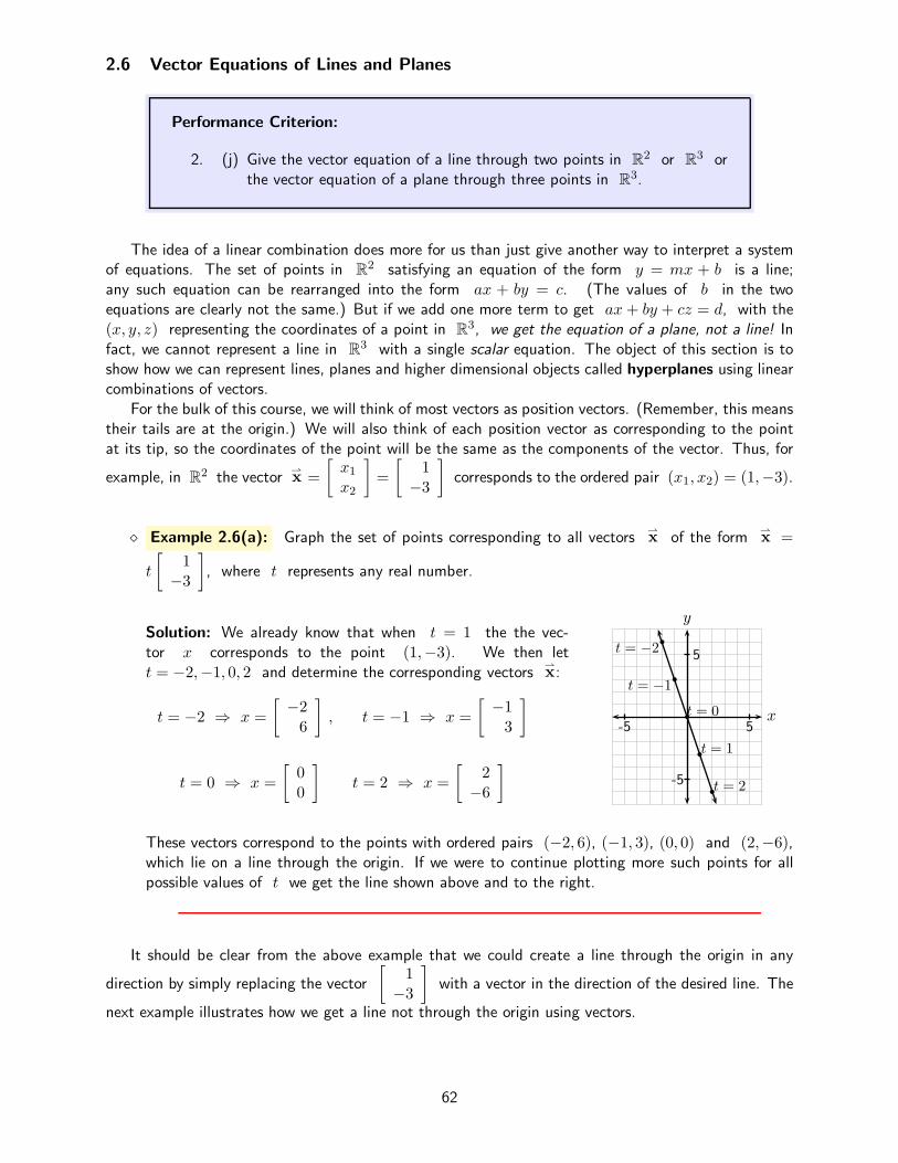
2.6 Vector Equations of Lines and Planes
Performance Criterion:
2. (j) Give the vector equation of a line through two points in R2 or R
3 orthe vector equation of a plane through three points in R
3.
The idea of a linear combination does more for us than just give another way to interpret a systemof equations. The set of points in R
2 satisfying an equation of the form y = mx + b is a line;any such equation can be rearranged into the form ax + by = c. (The values of b in the twoequations are clearly not the same.) But if we add one more term to get ax+ by + cz = d, with the(x, y, z) representing the coordinates of a point in R
3, we get the equation of a plane, not a line! Infact, we cannot represent a line in R
3 with a single scalar equation. The object of this section is toshow how we can represent lines, planes and higher dimensional objects called hyperplanes using linearcombinations of vectors.
For the bulk of this course, we will think of most vectors as position vectors. (Remember, this meanstheir tails are at the origin.) We will also think of each position vector as corresponding to the pointat its tip, so the coordinates of the point will be the same as the components of the vector. Thus, for
example, in R2 the vector
x =
[
x1x2
]
=
[
1−3
]
corresponds to the ordered pair (x1, x2) = (1,−3).
⋄ Example 2.6(a): Graph the set of points corresponding to all vectors
x of the form
x =
t
[
1−3
]
, where t represents any real number.
Solution: We already know that when t = 1 the the vec-tor x corresponds to the point (1,−3). We then lett = −2,−1, 0, 2 and determine the corresponding vectors
x:
t = −2 ⇒ x =
[
−26
]
, t = −1 ⇒ x =
[
−13
]
t = 0 ⇒ x =
[
00
]
t = 2 ⇒ x =
[
2−6
]
5
5
-5
-5
t = −2
t = −1t = 0
t = 1
t = 2
x
y
These vectors correspond to the points with ordered pairs (−2, 6), (−1, 3), (0, 0) and (2,−6),which lie on a line through the origin. If we were to continue plotting more such points for allpossible values of t we get the line shown above and to the right.
It should be clear from the above example that we could create a line through the origin in any
direction by simply replacing the vector
[
1−3
]
with a vector in the direction of the desired line. The
next example illustrates how we get a line not through the origin using vectors.
62

⋄ Example 2.6(b): Graph the set of points corresponding to all vectors
x of the form
x =[
23
]
+ t
[
−31
]
, where t represents any real number.
Solution: Performing the scalar multiplication by t and addingthe two vectors, we get
x =
[
2− 3t3 + t
]
.
These vectors then correspond to all points of the form (2 −3t, 3 + t). When t = 0 this is the point (2, 3) so our lineclearly passes through that point. Plotting the points obtainedwhen we let t = −1, 1, 2 and 3, we see that we will get theline shown to the right.
5
5
-5
-5
t = −1
t = 0
t = 1
t = 2
t = 3
P
Qx
y
Now let’s make two observations about the set of points represented by the set of all vectors
x =
[
23
]
+ t
[
−31
]
, where t again represents any real number. These vectors correspond to the
ordered pairs of the form (2−3t, 3+ t). Plotting these results in the line through the point (2, 3) and
in the direction of the vector
[
−31
]
. This is not a coincidence. Consider the line shown below and
to the left, containing the points P and Q. If we let
u =−−→OP and
v =−−→PQ, then the points
P and Q correspond to the vectors
u and
u +
v (in standard position, which you should assumewe mean from here on), as shown in the second picture. From this you should be able to see that if weconsider all the vectors
x defined by
x =
u +t
v as t ranges over all real numbers, the resultingset of points is our line! This is shown in the third picture, where t is given the values −1, 0, 1
2 and2.
O
P
Q
O
P
Q
u =−−→OP
v =−−→PQ
u +
v
O
PQ
u
v
−
v
u
u +(−1)
v
u +2
v
u + 1
2
v
O
P
Q
u
v
This may seem like an overly complicated way to describe a line,but with a little thought you should see that the idea translatesdirectly to three (and more!) dimensions, as shown in the pictureto the right. This is all summarized by the following.
63

Lines in R2 and R
3
The vector equation of a line through two points P and Q in R2 and R
3 (andeven higher dimensions) is
x =−−→OP + t
−−→PQ.
By this we mean that the line consists of all the points corresponding to the position
vectors
x as t varies over all real numbers. The vector−−→PQ is called the direction
vector of the line.
⋄ Example 2.6(c): Give the vector equation of the line in R2 through the points P (−4, 1) and
Q(5, 3).
Solution: We need two vectors, one from the origin out to the line, and one in the direction of
the line. For the first we will use−−→OP , and for the second we will use
−−→PQ = [9, 2]. We then
have
x =−−→OP + t
−−→PQ =
[
−41
]
+ t
[
92
]
,
where
x = [x1, x2] is the position vector corresponding to any point (x1, x2) on the line.
⋄ Example 2.6(d): Give a vector equation of the line in R3 through the points (−5, 1, 2) and
(4, 6,−3).
Solution: Letting P be the point (−5, 1, 2) and Q be the point (4, 6,−3), we get−−→PQ = 〈9, 5,−5〉. The vector equation of the line is then
x =−−→OP + t
−−→PQ =
−512
+ t
95−5
,
where
x = [x1, x2, x3] is the position vector corresponding to any point (x1, x2, x3) on theline.
The vector equation of a line is not unique! The first vector can be any point on the line, so it
could be the vector−−→OQ = [4, 6,−3] instead of [−5, 1, 2], for example. The second vector is simply
a direction vector, so can be any scalar multiple of−−→PQ = [9, 5,−5], including
−−→QP = [−9,−5, 5].
The same general idea can be used to describe a plane in R3. Before seeing how that works,
let’s define something and look at a situation in R2. We say that two vectors are parallel if one is a
scalar multiple of the other. Now suppose that
v and
w are two nonzero vectors in R2 that are
not parallel, as shown in Figure 2.6(a) on the next page, and let P be the randomly chosen point inR2 shown in the same picture. Figure 2.6(b) shows that a linear combination of
v and
w can beformed that gives us a vector s
v +t
w corresponding to the point P . In this case the scalar s ispositive and less than one, and t is positive and greater than one. Figures 2.6(c) and 2.6(d) show thesame thing for another point Q, with s being negative and t positive in that case. It should nowbe clear that any point in R
2 can be obtained in this manner.
64

v
wP
Figure 2.6(a)
s
vt
w
s
v +t
w
P
Figure 2.6(b)
u
vQ
Figure 2.6(c)
s
v
t
w
s
v +t
w
Q
Figure 2.6(d)
Now let
u,
v and
w be three vectors in R3, and consider the vector
x =
u +s
v +t
w, wheres and t are scalars that are allowed to take all real numbers as values. The vectors s
v +t
w alllie in the plane containing
v and
w. Adding
u “moves the plane off the origin” to where itpasses through the tip of
u (again, in standard position). This is probably best visualized by thinkingof adding s
v and t
w with the parallelogram method, then adding the result to
u with thetip-to-tail method. I have attempted to illustrate this to the left at the top of the next page, with thegray parallelogram being part of the plane created by all the points corresponding to the vectors
x.
u
s
v
t
w
s
v +t
w
x =
u +s
v +t
w
xy
z
P
Q
R
−−→OP
−−→PQ
−→PR
−−→PQ+
−→PR
x =−−→OP +
−−→PQ+
−→PR
xy
z
The same diagram above and to the right shows how all of the previous discussion relates to the planethrough three points P , Q and R in R
3. This leads us to the description of a plane in R3 given
at the top of the next page.
Planes in R3
The vector equation of a plane through three points P , Q and R in R3 (or
higher dimensions) is
x =−−→OP + s
−−→PQ+ t
−→PR.
By this we mean that the plane consists of all the points corresponding to theposition vectors
x as s and t vary over all real numbers.
⋄ Example 2.6(e): Give a vector equation of the plane in R3 through the points (2,−1, 3),
(−5, 1, 2) and (4, 6,−3). What values of s and t give the point R?
Solution: Letting P be the point (2,−1, 3), Q be (−5, 1, 2) and R be (4, 6,−3), we get
65

−−→PQ = [−7, 2,−1] and
−→PR = [2, 7,−6]. The vector equation of the plane is then
x =−−→OP + s
−−→PQ+ t
−→PR =
2−13
+ s
−72−1
+ t
27−6
,
where
x = [x1, x2, x3] is the position vector corresponding to any point (x1, x2, x3) on theplane. It should be clear that there are other possibilities for this. The first vector in the equationcould be any of the three position vectors for P , Q or R. The other two vectors could be anytwo vectors from one of the points to another.
The vector corresponding to point R is−−→OR, which is equal to
x =−−→OP +
−→PR (think about
that), so s = 0 and t = 1.
We now summarize all of the ideas from this section.
Lines in R2 and R
3, Planes in R3
Let
u and
v be vectors in R2 or R
3 with
v 6= 0. Then the set of pointscorresponding to the vector
x =
u + t
v as t ranges over all real numbers isa line through the point corresponding to
u and in the direction of
v. (So if
u =
0 the line passes through the origin.)
Let
u,
v and
w be vectors R3, with
v and
w being nonzero and not parallel.(That is, not scalar multiples of each other.) Then the set of points correspondingto the vector
x =
u + s
v + t
w as s and t range over all real numbers isa plane through the point corresponding to
u and containing the vectors
v and
w. (If
u =
0 the plane passes through the origin.)
Section 2.6 Exercises To Solutions
1. For each of the following, give the vector equation of the line or plane described.
(a) The line in R2 through the points P (3,−1) and Q(6, 0).
(b) The plane in R3 through the points P (3,−1, 4), Q(2, 6, 0) and R(−1, 0, 3).
(c) The line in R3 through the two points P (3,−1, 4) and Q(2, 6, 0).
(d) The line in R2 through the points (−1, 4) and (2, 5).
(e) The line in R2 through (−4, 3) and the origin. (Hint: Use the method of Example 2.6(c),
taking P to be (0, 0) and Q to be (−4, 3).)(f) The plane in R
3 through (−5, 1, 3), (2, 0, 4) and (1,−2, 3).(g) The line in R
3 through (2, 0,−1) and (1, 1, 3).
(h) The plane in R3 through (−4, 5, 1), (2, 2, 2) and the origin.
(i) The line in R3 through (1, 2, 3) and the origin.
66

2. Each of the lines or planes in the previous exercise constitutes a set of points in R2 or R
3.Which are sets closed under addition and scalar multiplication?
3. Give the equation of the three-dimensional hyperplane in R4 containing the points (−2, 1, 1, 5),
(3, 7,−5, 2), (4, 0, 5,−2) and (3,−5, 4, 7).
4. Consider the two points P (5,−1, 4) and Q(1, 1, 2) in R3.
(a) Give the vector equation of the line for which the value t = 0 for the parameter gives thepoint Q and t = 1 gives the point P .
(b) Give the vector equation of the line for which the value t = 0 for the parameter gives thepoint Q and t = −1 gives the point P .
(c) Give the vector equation of the line for which the value t = 0 for the parameter gives thepoint P and t = 2 gives the point Q.
5. Consider the two points P (−3, 1) and Q(2, 5) in R2.
(a) Give the “next” point with integer coordinates as one goes from P to Q.
(b) Give the vector equation for the line for which the parameter value t = 0 gives the pointP and t = 1 gives Q.
(c) What value of t in your equation from (b) gives the point you found in part (a)?
(d) Give the “next” point with integer coordinates as one goes from Q to P . What value ofthe parameter t in your equation from (b) gives this point?
6. Consider the three points P (1, 6,−2), Q(−5, 7, 4) and R(3, 0,−1) in R3. Give the vector
equation of plane in the form
x =
u + s
v + t
w for which s = 0 and t = 0 gives the pointQ, s = 0 and t = 1 gives R, and s = 1, t = 0 gives P .
7. Give the “next” three points on the line in R3 containing P (5,−1, 4) and Q(1, 1, 2), traveling
in the direction from P to Q.
8. Find another point in the plane containing P1(−2, 1, 5), P2(3, 2, 1) and P3(4,−2,−3). Showclearly how you do it. (Hint: Find and use the vector equation of the plane.)
9. “Usually” a vector equation of the form
x =
p + s
u + t
v gives the equation of a plane in R3.Answer the following first allowing any of
p,
u and
v to be the zero vector, then give answersassuming that none of them are zero.
(a) Under what conditions on
p and/or
u and/or
v would this be the equation of a line?
(b) Under what conditions on
p and/or
u and/or
v would this be the equation of a planethrough the origin?
67

2.7 Interpreting Solutions to Systems of Linear Equations
Performance Criterion:
2. (k) Write the solution to a system of equations in vector form and determinethe geometric nature of the solution.
We begin this section by considering the following two systems of equations.
3x1 − 3x2 + 3x3 = 9
2x1 − x2 + 4x3 = 7
3x1 − 5x2 − x3 = −3
x1 − x2 + 2x3 = 1
−3x1 + 3x2 − 6x3 = −32x1 − 2x2 + 4x3 = 2
The augmented matrices for these two systems reduce to the following matrices, respectively.
1 0 3 40 1 2 10 0 0 0
1 −1 2 10 0 0 00 0 0 0
Let’s look at the first system. x3 is a free variable, and x1 and x2 are leading variables. The generalsolution is x1 = −3t+ 4, x2 = −2t+ 1, x3 = t. Algebraically, x1, x2 and x3 are just numbers, but wecan think of (x1, x2, x3) as a point in R
3. The corresponding position vector is
x =
x1
x2
x3
=
4− 3t
1− 2t
t
=
4
1
0
+
−3t−2t
t
=
4
1
0
+ t
−3−21
We will call this the vector form of the solution to the system of equations. The beauty of expressingthe solutions to a system of equations in vector form is that we can see what the set of all solutions lookslike. In this case, the set of solutions is the set of all points in R
3 on the line through (4, 1, 0) andwith direction vector [−3,−2, 1].
⋄ Example 2.7(a): The general solution to the second system of equations is x1 = 1 + s − 2t,x2 = s, x3 = t. Express the solution in vector form and determine the geometric nature of thesolution set in R
3.
Solution: A process like the one just carried out leads to the general solution with position vector
x =
x1
x2
x2
=
1
0
0
+ s
1
1
0
+ t
−20
1
(Check to make sure that you understand how this was arrived at.) Here the set of solutions isthe set of all points in R
3 on the plane through (1, 0, 0) with direction vectors [1, 1, 0] and[−2, 0, 1].
68

Now recall that the three equations from this last example,
x1 − x2 + 2x3 = 1
−3x1 + 3x2 − 6x3 = −32x1 − 2x2 + 4x3 = 2
represent three planes in R3, and when we solve the system we are looking for all points in R
3 thatare solutions to all three equations. Our results tell us that the set of solution points in this case isitself a plane, which can only happen if all three equations represent the same plane. If you look atthem carefully you can see that the second and third equations are multiples of the first, so the pointssatisfying them also satisfy the first equation.
⋄ Example 2.7(b): The general solution to the second system of equations is x1 = 1 + s − 2t,x2 = s, x3 = t. Express the solution in vector form and determine the geometric nature of thesolution set in R
3.
Solution: A process like the one just carried out leads to the general solution with position vector
x =
x1
x2
x3
=
1
0
0
+ s
1
1
0
+ t
−20
1
(Check to make sure that you understand how this was arrived at.) Here the set of solutions isthe set of all points in R
3 on the plane through (1, 0, 0) with direction vectors [1, 1, 0] and[−2, 0, 1].
⋄ Example 2.7(c): Give the vector form of the solution to the system
3x2 − 6x3 − 4x4 − 3x5 = −5x1 − 3x2 + 10x3 + 4x4 + 4x5 = 2
2x1 − 6x2 + 20x3 + 2x4 + 8x5 = −8
Solution: The augmented matrix of the system reduces to
1 0 4 0 1 −30 1 −2 0 −1 1
0 0 0 1 0 2
We can see that x3 and x5 are free variables, and we can also see that x4 = 2. Lettingx5 = t and x3 = s, x2 = 1 + 2s+ t and x1 = −3− 4s− t. Therefore
x =
x1
x2
x3
x4
x5
=
−31
0
2
0
+ s
−42
1
0
0
+ t
−11
0
0
1
69

How do we interpret this result geometrically? The set of points (x1, x2, x3, x4, x5) represents atwo-dimensional plane in five-dimensional space. We could also have ended up with one, three or fourdimensional “plane”, often called a hyperplane, in five-dimensional space.
Section 2.7 Exercises To Solutions
1. For each of the following, a student correctly finds the given the general solution (x1, x2, x3) toa system of three equations in three unknowns. Give the vector form of the solution, then tellwhether the set of all particular solutions is a point, line or plane.
(a) x1 = s− t+ 5, x2 = s, x3 = t (b) x1 = 2t+ 5, x2 = t, x3 = −1
(c) x1 = s− 2t+ 5, x2 = s, x3 = t
2. In each of the following, the vector form of the solution to a system of linear equations is given.Give the dimension of the solution, and the dimension of the space it is in. For example you mightanswer “three-dimensional plane in five-dimensional space.”
(a)
x =
x1
x2
x3
x4
=
5
1
−14
+ r
3
7
1
−4
+ s
6
3
−108
+ t
1
1
1
1
(b)
x =
x1
x2
x3
x4
x5
= r
−31
0
2
0
+ s
−42
1
0
0
+ t
−11
0
0
1
(c)
x =
1
0
−31
0
2
0
+ t1
5
−3−42
1
0
0
+ t2
1
5
−11
0
0
1
+ t3
2
−51
0
3
9
3
+ t4
5
7
−4−21
−45
+ t5
3
1
−16
10
−41
(d)
x =
x1
x2
x3
x4
x5
=
4
−73
6
−1
+ t
2
0
−8−14
70

(e)
x =
x1
x2
x3
x4
=
1
1
1
1
+ s
3
7
1
−4
+ s
6
3
−108
(f)
x =
x1
x2
x3
x4
x5
x6
x7
= t1
1
5
−11
0
0
1
+ t2
2
−51
0
3
9
3
+ t3
5
7
−4−21
−45
+ t4
3
1
−16
10
−41
71

2.8 The Dot Product of Vectors, Projections
Performance Criteria:
3. (g) Find the dot product of two vectors, determine the length of a singlevector.
(h) Determine whether two vectors are orthogonal (perpendicular).
(i) Find the projection of one vector onto another, graphically or alge-braically.
The Dot Product and Orthogonality
There are two ways to “multiply” vectors, both of which you have likely seen before. One is calledthe cross product, and only applies to vectors in R
3. It is quite useful and meaningful in certainphysical situations, but it will be of no use to us here. More useful is the other method, called the dotproduct, which is valid in all dimensions.
Definition 2.8.1: Dot Product
Let
u= [u1, u2, ..., un] and
v= [v1, v2, ..., vn]. The dot product of
u and
v,denoted by
u · v, is given by
u · v= u1v1 + u2v2 + u3v3 + · · · + unvn
The dot product is useful for a variety of things. Recall that the length of a vector
v= [v1, v2, ..., vn] is
given by ‖
v ‖ =√
v21 + v22 + · · ·+ v2n =√
v · v. Note also that v21 + v22 + · · ·+ v2n =
v · v, which
implies that ‖
v ‖ =√
v · v. Perhaps the most important thing about the dot product is that thedot product of two vectors in R
2 or R3 is zero if, and only if, the two vectors are perpendicular. In
general, we make the following definition.
Definition 2.8.2: Orthogonal Vectors
Two vectors
u and
v in Rn are said to be orthogonal if, and only if,
u · v= 0.
⋄ Example 2.8(a): For the three vectors u =
5
−12
, v =
−13
4
and w =
2
−1−3
,
find
u · v,
u ·
w and
v ·
w. Are any of the vectors orthogonal to each other?
Solution: We find that
u · v= (5)(−1) + (−1)(3) + (2)(4) = −5 + (−3) + 8 = 0,
72

u ·
w= (5)(2) + (−1)(−1) + (2)(−3) = 10 + 1 + (−6) = 5,
v ·
w= (−1)(2) + (3)(−1) + (4)(−3) = −2 + (−3) + (−12) = −17From the first computation we can see that
u and
v are orthogonal.
Projections
Given two vectors
u and
v, we can create a new vector
w called the projection of
u onto
v,denoted by projv
u. This is a very useful idea, in many ways. Geometrically, we can find projv
u asfollows:
• Bring
u and
v together tail-to-tail.
• Sketch in the line containing
v, as a dashed line.
• Sketch in a dashed line segment from the tip of
u to the dashed line containing
v, perpendicularto that line.
• Draw the vector projv
u from the point at the tails of
u and
v to the point where thedashed line segment meets
v or the dashed line containing
v.
Note that projv
u is parallel to
v; if we were to find proju
v instead, the result would be parallelto
u in that case. The above steps are illustrated in the following example.
⋄ Example 2.8(b): For the vectors
u and
v shown to the right, find the projection
projv
u.
u
v
Solution: Following the above steps we get
u
v
=⇒
u
v
=⇒
u
v
=⇒
u
projv
u
Projections are a bit less intuitive when the angle between the two vectors is obtuse, as seen in thenext example.
73

⋄ Example 2.8(c): For the vectors
u and
v shown to the right, find
the projection proju
v.
v
u
Solution: We follow the steps again, noting that this time we are projecting
v onto
u:
v
u
=⇒
v
u
=⇒
v
u
=⇒
v
u
proju
v
Here we see that proju
v is in the direction opposite
u.
We will also want to know how to find projections algebraically:
Definition 2.8.3: The Projection of One Vector on Another
For two vectors
u and
v, the vector projv
u is given by
projv
u=
u · v
v · v
v
Note that since both
u ·
v and
v ·
v are scalars, so is
u · v
v · v. That scalar is then multiplied
times
v, resulting in a vector parallel
v. if the scalar is positive the projection is in the direction of
v, as shown in Example 2.8(b); when the scalar is negative the projection is in the direction oppositethe vector being projected onto, as shown in Example 2.8(c).
⋄ Example 2.8(d): For the vectors u =
5
−12
and v =
2
−1−3
, find proju
v.
Note that here we are projecting
v onto
u. first we find
v · u= (2)(5) + (−1)(−1) + (−3)(2) = 5 and
u · u= 52 + (−1)2 + 22 = 30
Then
proju
v=
v · u
u · u
u=5
30
5
−12
=
1
6
5
−12
=
56
−1613
74

As stated before, the idea of projection is extremely important in mathematics, and arises in situationsthat do not appear to have anything to do with geometry and vectors as we are thinking of them now.You will see a clever geometric use of vectors in one of the exercises.
Section 2.8 Exercises To Solutions
1. Consider the vectors
v=
[
−27
]
and
b=
[
13
]
.
(a) Draw a neat and accurate graph of
v and
b, with their tails at the origin, labeling each.
(b) Use the formula to find projb
v, with its components rounded to the nearest tenth.
(c) Add projb
v to your graph. Does it look correct?
2. For each pair of vectors v and b below, do each of the following
i) Sketch v and b with the same initial point.
ii) Find projb
v algebraically, using the formula for projections.
iii) On the same diagram, sketch the projb
v you obtained in part (ii). If it does not look theway it should, find your error.
iv) Find projb
v, and sketch it as a new sketch. Compare with your previous sketch.
(a) v =
[
31
]
, b =
[
5−2
]
(b) v =
[
−50
]
, b =
[
−21
]
(c) v =
[
31
]
, b =
[
−2−4
]
3. For each pair of vectors
u and
v, sketch projv
u. Indicate any right angles with the standardsymbol.
u
v
(a)
u
v(b)
u
v
(c)
u
v
(d)
(
u and
v are orthogonal)
75

3 Matrices and Vectors
Outcome:
3. Understand matrices, their algebra, and their action on vectors. Use matricesto solve problems. Understand the algebra of matrices.
Performance Criteria:
(a) Give the dimensions of a matrix. Identify a given entry, row or columnof a matrix.
(b) Identify matrices as square, upper triangular, lower triangular, symmetric,diagonal. Give the transpose of a given matrix; know the notation forthe transpose of a matrix.
(c) Add or subtract matrices when possible. Multiply a matrix by a scalar.
(d) Multiply a matrix times a vector, give the linear combination form of amatrix times a vector.
(e) Give a specific matrix that is multiplied times an arbitrary vector to obtaina given resulting vector.
(f) Express a system of equations as a coefficient matrix times a vectorequalling another vector.
(g) For a given matrix A and vector
b, find a vector
x for which
A
x =
b,
(h) Determine whether a matrix is a projection matrix, reflection matrix orrotation matrix, or none of these, by its action on a few vectors.
(i) Determine whether a vector is an eigenvector of a matrix. If it is, givethe corresponding eigenvalue.
(j) Know when two matrices can be multiplied, and know that matrix mul-tiplication is not necessarily commutative. Multiply two matrices “byhand.”
(k) Determine whether two matrices are inverses without finding the inverseof either.
(l) Find the inverse of a 2×2 matrix using the formula. Find the inverseof a matrix using the Gauss-Jordan method. Describe the Gauss-Jordanmethod for finding the inverse of a matrix.
(m) Solve a system of equations using an inverse matrix. Describe how touse an inverse matrix to solve a system of equations.
(n) Find the determinant of a 2×2 or 3×3 matrix by hand. Use a calculatorto find the determinant of an n× n matrix.
(o) Use the determinant to determine whether a system of equations has aunique solution.
(p) Determine whether a homogeneous system has more than one solution.
Continued on the next page.
76

Outcome:
3. Understand matrices, their algebra, and their action on vectors. Use matricesto solve problems. Understand the algebra of matrices.
Performance Criteria:
(q) Use Cramer’s rule to solve a system of equations.
(r) Give the geometric or algebraic representations of the inverse or squareof a rotation. Demonstrate that the geometric and algebraic versions arethe same
(s) Give the incidence matrix of a graph or digraph. Given the incidencematrix of a graph or digraph, identify the vertices and edges using correctnotation, and draw the graph.
(t) Determine the number of k-paths from one vertex of a graph to another.Solve problems using incidence matrices.
77

3.1 Introduction to Matrices
Performance Criteria:
3. (a) Give the dimensions of a matrix. Identify a given entry, row or columnof a matrix.
(b) Identify matrices as square, upper triangular, lower triangular, symmetric,diagonal. Give the transpose of a given matrix; know the notation forthe transpose of a matrix.
(c) Add or subtract matrices when possible. Multiply a matrix by a scalar.
A matrix is simply an array of numbers arranged in rows and columns. Here are some examples:
A =
[
1 2
2 3
]
, B =
−5 1
0 4
2 −3
, D =
3 0 0 0
0 4 0 0
0 0 5 0
0 0 0 6
, L =
1 0 0
−3 1 0
5 −2 1
We will always denote matrices with italicized capital letters. There should be no need to define therows and columns of a matrix. The number of rows and number of columns of a matrix are called itsdimensions. The second matrix above, B, has dimensions 3× 2, which we read as “three by two.”The numbers in a matrix are called its entries. Each entry of a matrix is identified by its row, thencolumn. For example, the (3, 2) entry of L is the entry in the 3rd row and second column, −2. Ingeneral, we will define the (i, j)th entry of a matrix to be the entry in the ith row and jth column.
There are a few special kinds of matrices that we will run into regularly:
• A matrix with the same number of rows and columns is called a square matrix. Matrices A,D and L above are square matrices.
• The entries that are in the same number row and column of a square matrix are called the diagonalentries of the matrix. For example, the diagonal entries of A are 1 and 3. All the diagonalentries taken together are called the diagonal of the matrix. (This ALWAYS refers to only thediagonal from upper left to lower right.)
• A square matrix with zeros “above” the diagonal is called a lower triangular matrix; L is anexample of a lower triangular matrix. Similarly, an upper triangular matrix is one whose entriesbelow the diagonal are all zeros. (Note that the words “lower” and “upper” refer to the triangularparts of the matrices where the entries are NOT zero.)
• A square matrix all of whose entries above AND below the diagonal are zero is called a diagonalmatrix. D is an example of a diagonal matrix. Any diagonal matrix is also both upper and lowertriangular.
• A diagonal matrix with only ones on the diagonal is called “the” identity matrix. We use theword “the” because in a given size there is only one identity matrix. We will soon see why it iscalled the “identity.”
• Given a matrix, we can create a new matrix whose rows are the columns of the original matrix.(This is equivalent to the columns of the new matrix being the rows of the original.) The new
78

matrix is called the transpose of the original. The transposes of the matrices B and L above aredenoted by BT and LT . They are the matrices
BT =
[ −5 0 2
1 4 −3
]
LT =
1 −3 5
0 1 −20 0 1
If a matrix a is m× n, then AT is n×m. Note that when a matrix is square, its transposeis obtained by “flipping the matrix over its diagonal.”
• Notice that AT = A. Such a matrix is called a symmetric matrix. One way of thinking ofsuch a matrix is that the entries across the diagonal from each other are equal. Matrix D is alsosymmetric, as is the matrix
1 5 0 −25 −4 7 3
0 7 0 −6−2 3 −6 −3
When discussing an arbitrary matrix A with dimensions m × n we refer to each entry as a,but with a double subscript with each to indicate its position in the matrix. The first number in thesubscript indicates the row of the entry and the second indicates the column of that entry:
A =
a11 a12 a13 · · · a1k · · · a1n
a21 a22 a23 · · · a2k · · · a2n...
......
...
aj1 aj2 aj3 · · · ajk · · · ajn...
......
...
am1 am2 am3 · · · amk · · · amn
Under the right conditions it is possible to add, subtract and multiply two matrices. We’ll savemultiplication for a little, but we have the following:
Definition 3.1.1: Adding and Subtracting Matrices
When two matrices have the same dimensions, they are added or subtracted byadding or subtracting their corresponding entries.
⋄ Example 3.1(a): Determine which of the matrices below can be added, and add those thatcan be.
A =
[
1 2
2 3
]
, B =
−5 1
0 4
2 −3
, C =
[ −7 4
1 5
]
Solution: B cannot be added to either A or C, but
A+ C =
[
1 2
2 3
]
+
[ −7 4
1 5
]
=
[ −6 6
3 8
]
79

It should be clear that A and C could be subtracted, and that A+C = C+A but A−C 6= C−A.
Definition 3.1.2: Scalar Times a Matrix
The result of a scalar c times a matrix A is the matrix each of whose entries arec times the corresponding entry of A.
⋄ Example 3.1(b): For the matrix A =
3 1 −1−2 8 56 −4 −3
, find 3A.
3A = 3
3 1 −1−2 8 56 −4 −3
=
9 3 −3−6 24 1518 −12 −9
Section 3.1 Exercises To Solutions
1. (a) Give the dimensions of matrices A, B and C in Exercise 3 below.
(b) Give the entries b31 and c23 of the matrices B and C in Exercise 3 below.
2. Give the names of the matrices at the top of the next page that are
(a) square (b) symmetric (c) diagonal
(d) upper triangular (e) lower triangular
A =
−4 0 02 6 0−1 5 3
B =
[
1 −4 3−4 5 2
]
C =
3 0 00 1 00 0 −5
D =
[
1 −4−4 5
]
E =
2 5 −3 10 4 0 20 0 −1 60 0 0 3
F =
2 7−1 46 5
G =
3 4 −5 04 1 7 0−5 7 −2 00 0 0 3
H =
[
3 14 5
]
J =
3 2 −12 1 3−1 3 −5
3. Give examples of each of the following types of matrices.
(a) lower triangular (b) diagonal
(c) symmetric (d) identity
(e) upper triangular but not diagonal (f) symmetric but without any zero entries
(g) symmetric but not diagonal (h) diagonal but not a multiple of an identity
80

4. Give the transpose of each matrix. Use the correct notation to denote the transpose.
A =
1 0 5−3 1 −24 7 0
B =
1 0−3 14 7
C =
1 0 −1 3−3 1 2 04 7 0 −2
D =
1 −31 21 4
5. Give all possible sums and differences of matrices from Exercise 4.
6. Consider the matrix below and to the left.
(a) What are some ways we could describe the matrix? Give all you can think of.
(b) Below and to the right the dotted lines indicate how the matrix can be broken into fourblocks, each of which is a 3 × 3 matrix. Give all ways you can think of to describe thematrix consisting of only the block in the upper left.
(c) Give all ways you can think of to describe the matrix consisting of the block in the lowerright.
(d) Give all ways you can think of to describe the matrices in the upper right and lower left.There is one more word to describe them that was not given in the section. What do youthink it is?
1
E− ν
E− ν
E0 0 0
− ν
E
1
E− ν
E0 0 0
− ν
E− ν
E
1
E0 0 0
0 0 01
G0 0
0 0 0 01
G0
0 0 0 0 01
G
1
E− ν
E− ν
E0 0 0
− ν
E
1
E− ν
E0 0 0
− ν
E− ν
E
1
E0 0 0
0 0 01
G0 0
0 0 0 01
G0
0 0 0 0 01
G
7. (a) For the matrix A =
[
1 23 4
]
, find the matrix B = A+AT .
(b) What kind of matrix is B?
81

3.2 Matrix Times a Vector
Performance Criteria:
3. (d) Multiply a matrix times a vector, give the linear combination form of amatrix times a vector.
(e) Give a specific matrix that is multiplied times an arbitrary vector to obtaina given resulting vector.
(f) Express a system of equations as a coefficient matrix times a vectorequalling another vector.
(g) For a given matrix A and vector
b, find a vector
x for which
A
x =
b.
Matrix Times a Vector
Multiplying a matrix times a vector is in some sense THE foundational operation of linear algebra.When we study algebra, trigonometry and calculus, what we are really interested in how functions acton numbers. In linear algebra we are interested in how matrices act on vectors. This action is usuallyreferred to as multiplication of a matrix times a vector, but we will be well served by remembering thatit is truly an action of a matrix on a vector.
Before getting into how to do this, we need to devise a useful notation. Consider the matrix
A =
a11 · · · a1n
a21 · · · a2n...
. . ....
am1 · · · amn
Each column of A, taken by itself, is a vector. We’ll refer to the first column as the vector
a∗1,with the asterisk * indicating that the row index will range through all values, and the 1 indicatingthat the values all come out of column one. Of course
a∗2 denotes the second column, and so on.Similarly,
a1∗ will denote the first row,
a2∗ the second row, etc. Technically speaking, the rows arenot vectors, but we’ll call them row vectors and we’ll call the columns column vectors. If we use justthe word vector, we will mean a column vector.
⋄ Example 3.2(a): Give
a2∗ and
a∗3 for the matrix A =
−5 3 4 −17 5 2 4
2 −1 −6 0
a2∗ =[
7 5 2 4]
and
a∗3 =
4
2
−6
A row vector can be multiplied times a column vector (only in that order) if they have the samenumber of components. To do this, we simply multiply each entry of the row vector times each entryof the column vector and add all the results. The result of a row vector times a column vector is thena single number. This is shown in the following example.
82

⋄ Example 3.2(b): Multiply
u =[
5 −3 2]
times
v =
−42
1
.
u
v = (5)(−4) + (−3)(2) + (2)(1) = −20 + (−6) + 2 = −24. Note that if
u was a true(column) vector, this would be
u · v.
Technically, the result −24 should be the 1 × 1 matrix [−24], but we are really only interested inthe above operation as it relates to taking a matrix times a vector. Once we are able to do that, thereis no need to do the above operation except as a part of the process of taking a matrix times a vector.We now define how to multiply a matrix times a vector.
Definition 3.2.1: Matrix Times a Vector
An m× n matrix A can be multiplied times a vector
x with n components.The result is a vector with m components, the ith component being the productof the ith row of A with
x, as shown below.
A
x =
a11 · · · a1n
a21 · · · a2n...
. . ....
am1 · · · amn
x1
x2...
xn
=
a11x1 + · · ·+ a1nxn
a21x1 + · · ·+ a2nxn...
am1x1 + · · ·+ amnxn
=
a1∗
x
a2∗
x
...
am∗
x
⋄ Example 3.2(c): Multiply
3 0 −1−5 2 4
1 −6 0
2
1
−7
.
3 0 −1−5 2 4
1 −6 0
2
1
−7
=
(3)(2) + (0)(1) + (−1)(−7)(−5)(2) + (2)(1) + (4)(−7)(1)(2) + (−6)(1) + (0)(−7)
=
13
−36−4
There is no need for the matrix multiplying a vector to be square, but when it is not, the resulting vectoris not the same length as the original vector:
⋄ Example 3.2(d): Find A
x for A =
[
7 −4 2
−1 0 6
]
and
x =
3
−51
.
A
x =
[
7 −4 2
−1 0 6
]
3
−51
=
[
(7)(3) + (−4)(−5) + (2)(1)
(−1)(3) + (0)(−5) + (6)(1)
]
=
[
43
3
]
83

We sometimes describe what we see in the above example by saying that the matrix A transforms the
vector
x =
3
−51
into the vector
[
433
]
. This emphasizes the fact that we are interested in a
matrix times a vector as more than just an algebraic computation.Note that, if a matrix A is 1 × n and
x is a vector with n components, the multiplication
x A can be performed, but such multiplication do not arise naturally in applications. We will alwaysmultiply a matrix times a vector, in that order, so we always write A
x rather than
xA.
Matrix Times a Vector Form of a System
We now see an example that has important implications.
⋄ Example 3.2(e): Multiply A =
1 −1 2
−3 4 −22 1 5
times the vector
x =
x1
x2
x3
.
A
x=
1 −1 2
−3 4 −22 1 5
x1
x2
x3
=
x1 − x2 + 2x3
−3x1 + 4x2 − 2x3
2x1 + x2 + 5x3
Consider now the system shown below and to the left:
x1 − x2 + 2x3 = 5
−3x1 + 4x2 − 2x3 = −12x1 + x2 + 5x3 = 2
x1 − x2 + 2x3
−3x1 + 4x2 − 2x3
2x1 + x2 + 5x3
=
5
−12
Because two vectors are equal if their corresponding components are equal, we can rewrite the systemin the form shown above and to the right and, as a result of Example 3.2(e), this leads to
1 −1 2
−3 4 −22 1 5
x1
x2
x3
=
5
−12
.
This is what we will refer to as the matrix times a vector form of a system of equations.
84

Definition 3.2.2 Matrix Times a Vector Form of a System
A systema11x1 + a12x2 + · · · + a1nxn = b1
a21x1 + a22x2 + · · · + a2nxn = b2...
am1x1 + am2x2 + · · · + amnxn = bm
of m linear equations in n unknowns can be written as a matrix times a vectorequalling another vector:
a11 a12 · · · a1na21 a22 · · · a2n
...am1 am2 · · · amn
x1x2...xn
=
b1b2...bm
We will refer to this as the matrix times a vector form of the system of equa-tions, and we express it compactly as A
x =
b.
⋄ Example 3.2(f): Give the matrix times vector form of the system3x1 + 5x2 = −1x1 + 4x2 = 2
.
Solution: The matrix times vector form of the system is
[
3 51 4
] [
x1x2
]
=
[
−12
]
.
Now we can solve the “inverse problem” of a matrix times a vector:
⋄ Example 3.2(g): Let A =
[
3 51 4
]
and
b =
[
4−1
]
. Find a vector
x =
[
x1x2
]
for
which A
x =
b.
Solution: We are trying to solve the matrix-vector equation
[
3 51 4
] [
x1x2
]
=
[
4−1
]
. This
is the matrix times a vector form of the system
3x1 + x2 = 4x1 + 4x2 = −1 ,
which we can solve by the addition method or row-reduction to obtain
x =
[
3−1
]
.
85

Linearity of the Action of a Matrix on a Vector
Multiplication of vectors by matrices has the following important properties, which are easily verified.
Theorem 3.2.3
Let A and B be matrices,
x and
y be vectors, and c be any scalar. Assumingthat all the indicated operations below are defined (possible), then
(a) A(
x +
y) = A
x +A
y (b) A(c
x) = c (A
x)
(c) (A+B)
x = A
x +B
x
We now come to a very important idea that depends on the first two properties of Theorem 3.2.3. Whenwe act on a mathematical object with another object, the object doing the “acting on” is often calledan operator. Some operators you are familiar with are the derivative operator and the antiderivativeoperator (indefinite integral), which act on functions to create other functions. Note that the derivativeoperator has the following two properties, for any functions f and g and real number c:
d
dx(f + g) =
df
dx+
dg
dx,
d
dx(cf) = c
df
dx
These are the same as the first two properties above for multiplication of a vector by a matrix. Amatrix can be thought of as an operator that operates on vectors (through multiplication). The firsttwo properties of multiplication of a vector by a matrix, as well as the corresponding properties of thederivative, are called the linearity properties. Both the derivative operator and the matrix multiplicationoperator are then called linear operators. This is why this subject is called linear algebra!
Linear Combination Form of a Matrix Times a Vector
There is another way to compute a matrix times a vector. It is not as efficient to do by hand as themethod implied by Definition 3.2.1, but it will be very important conceptually quite soon. Using ourearlier definition of a matrix A times a vector
x, we see that
A
x=
a11x1 + · · ·+ a1nxn
a21x1 + · · ·+ a2nxn...
am1x1 + · · ·+ amnxn
=
a11x1
a21x1...
am1x1
+
a21x2
a22x2...
am2x2
+ · · ·+
a1nxn
a2nxn...
amnxn
= x1
a11
a21...
am1
+ x2
a21
a22...
am2
+ · · · + xn
a1n
a2n...
amn
Let’s think about what the above shows. It gives us the result below, which is illustrated in Examples3.2(h) and (i).
86

Linear Combination Form of a Matrix Times a Vector
The product of a matrix A and a vector
x is a linear combination of the columnsof A, with the scalars being the corresponding components of
x.
⋄ Example 3.2(h): Give the linear combination form of
[
7 −4 2
−1 0 6
]
3
−51
.
[
7 −4 2
−1 0 6
]
3
−51
= 3
[
7
−1
]
− 5
[
−40
]
+ 1
[
2
6
]
⋄ Example 3.2(i): Give the linear combination form of
1 3 −23 7 1−2 1 7
x1x2x3
.
1 3 −23 7 1−2 1 7
x1x2x3
= x1
13−2
+ x2
371
+ x3
−217
Section 3.2 Exercises To Solutions
1. Multiply
1 0 −1−3 1 24 7 −2
5−12
and
[
3 −4 0−1 5 1
]
−152
by hand.
2. Multiply each of the following by hand, when possible. Some are on the next page.
(a)
[
3 −15 2
] [
−41
]
(b)
[
1 −5 26 3 −4
]
10−3
(c)
[
1 −5 26 3 −4
] [
35
]
(d)
1 6−5 32 −4
[
35
]
(e)
7 −2 0 41 5 3 −32 1 −1 5−3 7 2 1
−4132
(f)
1 0 −52 2 3−4 7 1
2−31
87

3. Give each of the products from Exercise 2 in linear combination form.
4. Give the product
a11 a12 a13a21 a22 a23a31 a32 a33
x1x2x3
as
(a) a single vector (b) a linear combination of vectors
5. (a) Find a matrix A such that A
[
x1x2
]
=
[
3x1 − 5x2x1 + x2
]
.
(b) Find a matrix B such that B
[
x1x2
]
=
x1 + 3x22x1 − x25x1 + 4x2
.
(c) Find a matrix C such that C
x1x2x3
=
2x1 + 4x2 − x3−5x1 + x2 + 2x3
x1 + 3x2
.
(d) Find a matrix D such that D
x1x2x3
=
[
x1 + x3x1 − x2 − x3
]
.
6. Give the matrix times a vector form of each system:
(a) (b)x + y − 3z = 1
−3x+ 2y − z = 7
2x + y − 4z = 0
5x1 + x3 = −12x2 + 3x3 = 0
2x1 + x2 − 4x3 = 2
(c) (d)b+ 0.5m = 8.1
b+ 1.0m = 6.9
b+ 1.5m = 6.2
b+ 2.0m = 5.3
b+ 2.5m = 4.5b+ 3.0m = 3.8
b+ 3.5m = 3.0
x1 − 4x2 + x3 + 2x4 = −13x1 + 2x2 − x3 − 7x4 = 0
−2x1 + x2 − 4x3 + x4 = 2
7. For each part of this exercise, find a vector
x for which A
x =
b for the A and
b given.
(a) (b)
A =
3 −1 5
2 0 2
−1 4 −3
,
b =
3
−21
A =
[
1 −35 −2
]
,
b =
[
2429
]
(c) (d)
A =
1 2.1
1 2.7
1 3.2
1 3.9
,
b =
2.54
2.78
2.98
3.26
A =
1 3 0 0
3 1 2 0
0 2 1 3
0 0 3 1
,
b =
13
19
11
7
88

8. The relationship between stress and strain in a small cube of solid material can be expressed bythe matrix equation
1
E− ν
E− ν
E0 0 0
− ν
E
1
E− ν
E0 0 0
− ν
E− ν
E
1
E0 0 0
0 0 01
G0 0
0 0 0 01
G0
0 0 0 0 01
G
σxx
σyy
σzz
τxy
τyz
τzx
=
ǫxx
ǫyy
ǫzz
γxy
γyz
γzx
where
E is elastic modulus
G is shear modulus
ν is Poisson’s ratio
ǫ is normal strain
γ is shear strain
σ is normal stress
τ is shear stress
and the subscripts indicate faces of the cube and directions of forces. The vector being multipliedis the stress vector, and the right hand side is the strain vector.
(a) Give the relationship expressed by the product of the second row of the matrix times thestress vector.
(b) Give an expression for the ǫzz strain in terms of the three stresses σxx, σyy, σzz and theparameters E and ν.
(c) Give the relationship between τzx and γzx.
(d) The coefficient matrix is what we call a block matrix made up of blocks, each of which is asmaller matrix. In this case there are four 3× 3 matrices, two of which are zero matrices.Each of the nonzero blocks is multiplied by only a portion of the stress vector and gives onlya portion of the strain vector. Write the two matrix equations for the nonzero blocks.
89

3.3 Actions of Matrices on Vectors: Transformations in R2
Performance Criteria:
3. (h) Determine whether a matrix is a projection matrix, reflection matrix orrotation matrix, or none of these, by its action on a few vectors.
(i) Determine whether a vector is an eigenvector of a matrix. If it is, givethe corresponding eigenvalue.
Most of the mathematics that you have studied revolves around the idea of a function, which is simplya rule that assigns to every number in the domain of the function another number. There need not beany logic to how this is done, but usually there is, and that logic is seen in the fact that the function isgiven as some sort of specific relationship, like
f(x) = x2 − 5x+ 2 , y =√x+ 3 , g(t) = 3 sin(2t− 5) , h(x) = lnx.
(The last two of these are sort of redundant, in the sense that they are built out of other functions, sineand the natural logarithm.) For those who are visually or mechanically inclined, a function can also bethought of as a “machine,” commonly named f , whose input is a number x and output is someother number y. We write y = f(x) and say “y equals f of x” to indicate that y is the resultof the function f acting on x. This is shown in the picture below and to the left.
f
x
y = f(x)
A
u
v= A
u
When we multiply a vector by a matrix, the result is another vector - this is essentially the sameidea as a function, but with vectors playing the role of numbers and a matrix taking the place of thefunction. This is shown in the picture above and to the right. We should really think of a matrixtimes a vector as the matrix acting on the vector to create another vector. We sometimes say that thematrix A transforms the original vector
u to the new one
v= A
u. This happens by the purelycomputational means that you learned in the previous section.
One powerful tool in the study of any function is its graphical representation. Unfortunately, it isdifficult to graphically represent the action of a matrix on all vectors - we instead must picture theaction of a matrix on vectors one or two vectors at a time. Even that is difficult with vectors in R
3 andimpossible in higher dimensions. Let’s see how we do it in R
2. Suppose that we have the matrix andvectors
90

A =
[
3 −12 1
]
,
u=
[
13
]
,
v=
[
−21
]
2
-3
-5
u
v
A
u
A
v
x
y
for which
A
u=
[
05
]
, A
v=
[
−7−3
]
.
The graph to the right shows the vectors
u,
v, A
u andA
v, and we can see the result of A acting on
u and
v. The two attributes of any vector are of course mag-nitude and direction, and we can see that A alteredthe magnitude and the direction of both vectors, butapparently not in any special way.
In general, when a matrix acts on a vector the resulting vector will have a different magnitude anddirection than the original vector, with the change in magnitude and direction being different for mostvectors. There are a few notable exceptions to this:
• The matrix that acts on a vector without actually changing it at all is called the identity matrix.Clearly, then, when the identity matrix acts on a vector, neither the direction or magnitude ischanged.
• A matrix that rotates every vector in R2 through a fixed angle θ is called a rotation matrix. In
this case the direction changes, but not the magnitude. (Of course the direction doesn’t changeif θ = 0 and, in some sense, if θ = 180. In the second case, even though the direction isopposite, the resulting vector is still just a scalar multiple of the original.)
• For most matrices there are certain vectors, called eigenvectors whose directions don’t change(other than perhaps reversing) when acted on by by the matrix under consideration. In thosecases, the effect of multiplying such a vector by the matrix is the same as multiplying the vectorby a scalar. This has very useful applications.
In the following exercises you will see rotation matrices and eigenvectors, along with some other matricesthat do interesting things to vectors geometrically.
Section 3.2 Exercises
For the following exercises you will be multiplying each of several vectors by a given matrix and tryingto see what the matrix does to the vectors. This can be pretty tedious by hand, so I would suggest thatyou use the UCSMP Polygon Plotter that you can link to from the class web page (or find with a websearch for “UCSMP polygon plotter”). You will need to enter each vector as a position vector from theorigin, and then transform it by the transformation matrix you are working with. Here’s how you do allthat:
• Under ”Enter New” you are asked “How Many Points”. Enter 2, meaning you are creating apolygon with only two vertices (a line segment!).
• Below that you are to describe your polygon as a “matrix.” The first column should be zeros, andthe second column should be the components of your vector. (The first column is the coordinatesof the initial point, and the second column is the coordinates of the terminal point.)
• Once you put the values in for the vector, click “Enter” and you should see your vector, in red.
91

• Enter your transformation matrix. For the ones with with entries containing roots, use theirdecimal representations rounded to the thousandth’s place. Fractions may be entered as theyare.
• Once you have entered the transformation matrix, click “Transform!” You will see the result ofthe transformation as a vector in black.
• If you now look below “Select Polygon:” you will see your vector under “Preimage: AB,” andthe result of the transformation as “Image: A’B’.”
• To multiply another vector by the same transformation, enter the new vector and click “En-ter” again, followed by “Transform!”
• To repeat all this with a different transformation matrix, click “Clear Grid” at the bottom andstart over.
1. Let A =
[
3 −1−4 0
]
,
u =
[
1
1
]
,
v =
[
−12
]
,
w =
[
0
2
]
.
(a) Find A
u, A
v and A
w by hand. Check your answers with the polygon plotter.
(b) Plot and label
u,
v,
w, A
u, A
v and A
w on one R2 coordinate grid. Label each
vector by putting its name near its tip.
You should not see any special relationship between the vectors
x and A
x (where
x is torepresent any vector) here.
2. Let B =
[√32 −1
2
12
√32
]
,
u=
[
4
0
]
,
v=
[
−31
]
,
w=
[
3
4.5
]
.
(a) Plot and label
u,
v,
w, B
u, B
v and B
w on one R2 coordinate grid. Label each
vector by putting its name near its tip.
(b) You should be able to see that B does not seem to change the length of a vector. To verifythis, find ‖
w ‖ and ‖B
w ‖ to the nearest hundredth.
(c) What does the matrix B seem to do to every vector? Think about the two attributesof any vector, direction and magnitude.
(d) The entries of B should look familiar to you. What is special about 12 and
√32 ?
3. Let C =
[
1625
1225
1225
925
]
,
u=
[
4
0
]
,
v=
[
−31
]
,
w=
[
4.5
6
]
.
(a) Plot and label
u,
v,
w, C
u, C
v and C
w on one R2 coordinate grid.
(b) What does the matrix C seem to do to every vector? (Does the magnitude change? Doesthe direction change?)
92

(c) Try C times
[
−4−3
]
and
[
3
−4
]
. Hmmm...
(d) Can you see the role of the entries of the matrix here?
4. Let D =
[
725
2425
2425 − 7
25
]
,
u=
[
4
0
]
,
v=
[
−31
]
,
w=
[
4.5
6
]
.
(a) Plot and label
u,
v,
w, D
u, D
v and D
w on one R2 coordinate grid.
(b) What does the matrix D seem to do to every vector? (Does the magnitude change? Doesthe direction change?)
(c) Try D times
[
−4−3
]
and
[
3
−4
]
. Hmmm...
(d) Can you see the role of the entries of the matrix here?
5. Again let A =
[
3 −1−4 0
]
, (see Exercise 1) but let
u=
[
−11
]
,
v=
[
1
2
]
,
w=
[
1
4
]
.
(a) Plot and label
u,
v,
w, A
u, A
v and A
w on one R2 coordinate grid.
(b) For one of the vectors, there should be no apparent relationship between the vector andthe result when it is multiplied by the matrix. Discuss what happened to the direction andmagnitude of each of the other two vectors when the matrix acted on it.
(c) Pick one of your two vectors for which something special happened and multiply it by three,and multiply the result by A; what is the effect of multiplying by A in this case?
(d) Pick the other special vector, multiply it by five, then by A. What effect does multiplyingby A have on the vector?
93

3.4 Multiplying Matrices
Performance Criteria:
3. (j) Know when two matrices can be multiplied, and know that matrix mul-tiplication is not necessarily commutative. Multiply two matrices “byhand.”
When two matrices have appropriate sizes they can be multiplied by a process you are about to see.Although the most reliable way to multiply two matrices and get the correct result is with a calculatoror computer software, it is very important that you get quite comfortable with the way that matricesare multiplied. That will allow you to better understand certain conceptual things you will encounterlater.
The process of multiplying two matrices is a bit clumsy to describe, but I’ll do my best here. First Iwill try to describe it informally, then I’ll formalize it with a definition based on some special notation.To multiply two matrices we just multiply each row of the first with each column of the second as wedid when multiplying a matrix times a vector, with the results becoming the elements of the secondmatrix. Here is an informal description of the process:
(1) Multiply the first row of the first matrix times the first column of the second. The result is the(1,1) entry (first row, first column) of the product matrix.
(2) Multiply the first row of the first matrix times the second column of the second. The result is the(1,2) entry (first row, second column) of the product matrix.
(3) Continue multiplying the first row of the first matrix times each column of the second to fill outthe first row of the product matrix, stopping after multiplying the first row of the first matrixtimes the last column of the second matrix.
(4) Begin filling out the second row of the product matrix by multiplying the second row of the firstmatrix times the first column of the second matrix to get the (2,1) entry (second row, first column)of the product matrix.
(5) Continue multiplying the second row of the first matrix times each column of the second until thesecond row of the product matrix is filled out.
(6) Continue multiplying each row of the first matrix times each column of the second until the lastrow of the first has been multiplied times the last column of the second, at which point the productmatrix will be complete.
Note that for this to work the number of columns of the first matrix must be equal the number of rowsof the second matrix. Let’s look at an example.
⋄ Example 3.4(a): For A =
−5 1
0 4
2 −3
and B =
[
1 2
7 3
]
, find the product AB.
Video Example
94

Solution:
AB =
−5 1
0 4
2 −3
[
1 2
7 3
]
=
−5(1) + 1(7) −5(2) + 1(3)
0(1) + 4(7) 0(2) + 4(3)
2(1) + (−3)(7) 2(2) + (−3)(3)
=
2 −728 12
−19 −5
In order to make a formal definition of matrix multiplication, we need to remember the specialnotation from Section 3.2 for rows and columns of a matrix. Given a matrix
A =
a11 a12 · · · a1n
a21 a22 · · · a2n...
......
am1 am2 · · · amn
,
we refer to, for example the third row as
a3∗. Here the first subscript 3 indicates that we areconsidering the third row, and the ∗ indicates that we are taking the elements from the third row inall columns. Therefore
a3∗ refers to a 1× n matrix. Similarly,
a∗2 is the vector that is the secondcolumn of A. So we have
a3∗ =[
a31 a32 · · · a3n]
a∗2 =
a12a22...
a2m
A 1 × n matrix like
a3∗ can be thought of like a vector; in fact, we sometimes call such a matrixa row vector. Note that the transpose of such a vector is a column vector. We then define a productlike product
ai∗
b∗j by
ai∗
b∗j= ai1b1j + ai2b2j + ai3b3j + · · · + ainbnj =n∑
k=1
aikbkj
This is the basis for the following formal definition of the product of two matrices.
95

Definition 3.4.1: Matrix Multiplication
Let A be an m× n matrix whose rows are the vectors
a1∗,
a2∗, ...,
am∗ andlet B be an n×p matrix whose columns are the vectors
b∗1,
b∗2, ...,
b∗p. ThenAB is the m× p matrix
AB =
a11 a12 · · · a1n
a21 a22 · · · a2n...
.... . .
...
am1 am2 · · · amn
b11 b12 · · · b1p
b21 b22 · · · b2p...
.... . .
...
bn1 bn2 · · · bnp
=
a1∗
a2∗...
am∗
[
b∗1
b∗2
b∗3 · · ·
b∗p ]
=
a1∗
b∗1
a1∗
b∗2 · · ·
a1∗
b∗p
a2∗
b∗1
a2∗
b∗2 · · ·
a2∗
b∗p...
.... . .
...
am∗
b∗1
am∗
b∗2 · · ·
am∗
b∗p
For the above computation to be possible, products in the last matrix.This impliesthat the number of columns of A must equal the number of rows of B.
⋄ Example 3.4(b): For C =
−5 1 −27 0 4
2 −3 6
and D =
1 2 −1−3 −7 0
5 2 3
, find CD and
DC.
Solution:
CD =
−5 1 −27 0 4
2 −3 6
1 2 −1−3 −7 0
5 2 3
=
−5− 3− 10 −10− 7− 4 5 + 0− 6
7 + 0 + 20 14 + 0 + 8 −7 + 0 + 12
2 + 9 + 30 4 + 21 + 12 −2 + 0 + 18
=
−18 −21 −127 22 5
41 37 16
DC =
1 2 −1−3 −7 0
5 2 3
−5 1 −27 0 4
2 −3 6
=
7 4 0
−34 −3 −22−5 −4 16
We want to notice in the last example that CD 6= DC! This illustrates something very important:
96

Matrix multiplication is not necessarily commutative! That is, given twomatrices A and B, it is not necessarily true that AB = BA. It is possible,but is not “usually” the case. In fact, one of AB and BA might exist andthe other not.
This is not just a curiosity; the above fact will have important implications in how certain computationsare done. The next example, along with Example 3.4(a), shows that one of the two products mightexist and the other not.
⋄ Example 3.4(c): For the same matrices A =
−5 1
0 4
2 −3
and B =
[
1 2
7 3
]
from
Example 3.4(a), find the product BA.
Solution: When we try to multiply BA =
[
1 2
7 3
]
−5 1
0 4
2 −3
it is not even possible. We
can’t find the dot product of a row of B with a column of A because, as vectors, they don’thave the same number of components. Therefore the product BA does not exist.
⋄ Example 3.4(d): For I2 =
[
1 0
0 1
]
, C =
[
3 0
0 3
]
and B =
[
1 2
7 3
]
, find the products
I2B, BI2, CB and BC.
Solution:
I2B = BI2 =
[
1 2
7 3
]
, CB = BC =
[
3 6
21 9
]
The notation I2 here means the 2× 2 identity matrix. Note that when it is multiplied by anothermatrix A on either side the result is just the matrix A.
Let’s take a minute to think a bit more about the idea of an “identity.” In the real numbers we sayzero is the additive identity because adding it to any real number a does not change the value of thenumber:
a+ 0 = 0 + a = a
Similarly, the number one is the multiplicative identity:
a× 1 = 1× a = a
Here the symbol × is just multiplication of real numbers. When we talk about an identity matrix,we are talking about a multiplicative identity, like the number one. There is no confusion because eventhough there are matrices that could be considered to be additive identities, they are not useful, so wedon’t consider them. When the size of the identity matrix is clear from the context, which is almostalways the case, we omit the subscript and just write I.
97

There are many other special and/or interesting things that can happen when multiplying twomatrices. Here’s an example that shows that we can take powers of a matrix if it is a square matrix.
⋄ Example 3.4(e): For the matrix A =
3 1 −1−2 8 56 −4 −3
, find A2 and A3.
Solution:
A2 = AA =
3 1 −1−2 8 56 −4 −3
3 1 −1−2 8 56 −4 −3
=
1 15 58 42 278 −14 −17
A3 = AA2 =
3 1 −1−2 8 56 −4 −3
1 15 58 42 278 −14 −17
=
3 101 59102 236 121−50 −36 −
In Section 3.1 we saw that a scalar times a matrix is defined by multiplying each entry of the matrixby the scalar. With a little thought the following should be clear:
Theorem 3.4.2
Let A and B be matrices for which the product AB is defined, and let c beany scalar. Then
c(AB) = (cA)B = A(cB)
Note this carefully - when multiplying a product of two matrices by a scalar, we can instead multiplyone or the other, but NOT BOTH of the two matrices by the scaler, then multiply the result with theremaining matrix.
Although one can do a great deal of study of matrices themselves, linear algebra is primarily concernedwith the action of matrices on vectors. The following simple result is extremely important conceptually:
Theorem 3.4.3
Let A and B be matrices and
x a vector. Assuming that all the indicatedoperations below are defined (possible), then
(AB)
x= A(B
x)
The following illustrates the difference between (AB)
x and A(B
x) from a computational standpoint.
⋄ Example 3.4(g): For the matrices A =
[
1 −1−2 5
]
and B =
[
4 −37 0
]
and the vector
x =
[
3−6
]
, find (AB)
x and A(B
x).
98

Solution: Be sure to note the difference between the how the two calculations are performed,along with the fact that the resluts are the same:
(AB)
x=
([
1 −1−2 5
] [
4 −37 0
])[
3−6
]
=
[
−3 −327 6
] [
3−6
]
=
[
945
]
A(B
x) =
[
1 −1−2 5
]([
4 −37 0
] [
3−6
])
=
[
1 −1−2 5
] [
3021
]
=
[
945
]
Let’s now continue the analogy between functions and multiplication of a vector by a matrix. Con-sider the functions
f(x) = x2 and g(x) = 2x− 1.
Suppose that we wanted to apply g to the number three, and then apply f to the result. We showthis symbolically by
f[
g(3)]
= f[
2(3)− 1]
= f [5] = 25.
We can form a new function called the composition of f and g, f g. This function is defined forany value of x by
(f g)(x) = f[
g(x)]
.
In the case of our particular f and g the composition is
(f g)(x) = f[
g(x)]
= f [2x− 1] = (2x− 1)2 = 4x2 − 4x+ 1,
and(f g)(3) = 4(3)2 − 4(3) + 1 = 36− 12 + 1 = 25,
showing that f g does indeed act on the number three just as f and g did in sequence. Let’sreiterate - f g is a single new function that is equivalent to performing g followed by f , in thatorder. If we were to perform the two functions on the number three, but in the opposite order, we wouldget
g[
f(3)]
= g[
32]
= g[9] = 2(9) − 1 = 17.
We also see that(g f)(x) = g
[
f(x)]
= g[x2] = 2x2 − 1,
so the functions f g and g f are not the same!Now Theorem 3.4.3 tells us that, for two matrices A and B and any vector
x,
(AB)
x= A(B
x)
when all of the operations are defined. Here A and B can be thought of like the functions f andg above, except they act on vectors rather than numbers. The product AB is like the compositionf g - it is a single matrix whose action
x is equivalent to B acting on
x, and then A acting onthe result B
x. The fact that CD is not usually equal to DC for two matrices C and D for whichboth CD and DC exist (see Example 3.4(b)) is analogous to the fact that the two compositionsf g and g f of two functions f and g are not generally the same.
99

Section 3.4 Exercises To Solutions
1. Multiply (a)
[
2 −1−3 4
] [
4 15 −1
]
and (b)
1 2 −1−3 4 12 −1 3
−2 4 13 −5 −10 1 2
by
hand.
2. For the following matrices, there are THIRTEEN multiplications possible, including squaring someof the matrices. Find and do as many of them do as many of them as you can. When writingyour answers, tell which matrices you multiplied to get any particular answer. For example, it ISpossible to multiply A times B (how about B times A?), and you would then write
AB =
[
−10 0 25
−14 21 −4
]
to give your answer. Now you have twelve left to find and do.
A =
[
0 5
−3 1
]
B =
[
4 −7 3
−2 0 5
]
C =
−54−7
D =
6 0 3
−5 4 2
1 1 0
E =
[
5 −1 2]
F =
[
2 −16 9
]
3. Fill in the blanks:
−5 1 3
2 4 0
1 −1 −6
6 0 −1−5 7 2
−4 1 3
=
∗ ∗ ∗∗ ∗
∗ ∗
4. Suppose that A =
a11 a12 a13 · · ·a21 a22
a31. . .
...
is a 5× 5 matrix. Write an expression for the
third row, second column entry of A2.
5. In the previous section you found that the matrix P =
[
1625
1225
1225
925
]
projects every vector in
R2 onto the line through the origin and the point (4, 3). If we wish to calculate P 2 we can
apply Theorem 3.4.2 to factor 125 out of each copy of the matrix, multiply the resulting matrices
with integer entries, then multiply the product of the two 125 scalars back in at the end. Do
this using your calculator for multiplying numbers, but not the actual matrix multiplication, andreduce the entries when you are done. The result may surprise you a bit!
100

6. Let A =
−5 1
0 4
2 −3
.
(a) Give AT , the transpose of A.
(b) Find ATA and AAT . Are they the same (equal)?
(c) Your answers to (b) are special in two ways. What are they? (What I’m looking for here istwo of the special types of matrices described in Section 3.1.)
101

3.5 Inverse Matrices
Performance Criteria:
3. (k) Determine whether two matrices are inverses without finding the inverseof either.
(l) Find the inverse of a 2×2 matrix using the formula. Find the inverseof a matrix using the Gauss-Jordan method. Describe the Gauss-Jordanmethod for finding the inverse of a matrix.
(m) Solve a system of equations using an inverse matrix. Describe how touse an inverse matrix to solve a system of equations.
Inverse Matrices
Let’s begin with an example!
⋄ Example 3.5(a): Find AC and CA for A =
[
5 72 3
]
and C =
[
3 −7−2 5
]
.
Solution:
AC =
[
5 72 3
] [
3 −7−2 5
]
=
[
1 00 1
]
, CA =
[
3 −7−2 5
] [
5 72 3
]
=
[
1 00 1
]
We see that AC = CA = I2!
Now let’s remember that the identity matrix is like the number one for multiplication of numbers. Notethat, for example, 1
5 · 5 = 5 · 15 = 1. This is exactly what we are seeing in the above example. We saythe numbers 5 and 1
5 are multiplicative inverses, and we say that the matrices A and C aboveare inverses of each other.
Definition 3.5.1 Inverse Matrices
Suppose that for matrices A and B we have AB = BA = I, with the sizeof the identity being the same in both cases. Then we say that A and B areinverse matrices.
Notationally we write B = A−1 or A = B−1, and we will say that A and B are invertible. Notethat in order for us to be able to do both multiplications AB and BA, both matrices must be squareand of the same dimensions. It also turns out that that to test two square matrices to see if they areinverses we only need to multiply them in one order:
Theorem 3.5.2 Test for Inverse Matrices
To test two square matrices A and B to see if they are inverses, compute AB.If it is the identity, then the matrices are inverses.
102

Here are a few notes about inverse matrices:
• Not every square matrix has an inverse, but “many” do. If a matrix does have an inverse, it issaid to be invertible.
• The inverse of a matrix is unique, meaning there is only one.
• Matrix multiplication IS commutative for inverse matrices.
Two questions that should be occurring to you now are
1) How do we know whether a particular matrix has an inverse?
2) If a matrix does have an inverse, how do we find it?
There are a number of ways to answer the first question; here is one:
Theorem 3.5.3 Test for Invertibility of a Matrix
A square matrix A is invertible if, and only if, rref (A) = I.
Finding Inverse Matrices
Here is the answer to the second question above in the case of a 2× 2 matrix:
Theorem 3.5.4 Inverse of a 2× 2 Matrix
The inverse of a 2× 2 matrix A =
[
a b
c d
]
is A−1 =1
ad− bc
[
d −b−c a
]
.
⋄ Example 3.5(b): Find the inverse of A =
[
−2 71 −5
]
.
Solution:
A−1 =1
(−2)(−5)− (1)(7)
[
−5 −7−1 −2
]
=1
3
[
−5 −7−1 −2
]
=
[
−53 −7
3
−13 −2
3
]
Before showing how to find the inverse of a larger matrix we need to go over the idea of augmentinga matrix with a vector or another matrix. To augment a matrix A with a matrix B, both matricesmust have the same number of rows. A new matrix, denoted [A |B ] is formed as follows: the firstrow of [A |B ] is the first row of A followed by the first row of B, and every other row in [A |B ] isformed the same way.
103

⋄ Example 3.5(c): Let A =
−5 1 −27 0 4
2 −3 6
, B =
9 1
−1 8
−6 −3
and
x=
−710
4
.
Give the augmented matrices [ A |
x ] and [A |B ].
Solution:[ A |
x ] =
−5 1 −2 −77 0 4 10
2 −3 6 4
, [A |B ] =
−5 1 −2 9 1
7 0 4 −1 8
2 −3 6 6 −3
Gauss-Jordan Method for Finding Inverse Matrices
Let A be an n×n invertible matrix and In be the n×n identity matrix. Formthe augmented matrix [A | In ] and find rref ([A | In ]) = [ In |B ]. (The resultof row-reduction will have this form.) Then B = A−1.
⋄ Example 3.5(d): Find the inverse of A =
2 3 0
1 −2 1
2 0 1
, if it exists.
Solution: We begin by augmenting with the 3×3 identity: [A | I3 ] =
2 3 0 1 0 0
1 −2 1 0 1 0
2 0 1 0 0 1
.
Row reducing then gives
1 0 0 2 3 −30 1 0 −1 −2 2
0 0 1 −4 −6 7
, so A−1 =
2 3 −3−1 −2 2
−4 −6 7
.
The above example is a bit unusual; the inverse of a randomly generated matrix will usually containfractions.
⋄ Example 3.5(e): Find the inverse of B =
1 −1 2
1 2 −10 2 −2
, if it exists.
Solution: We compute
[B | In ] =
1 −1 2 1 0 0
1 2 −1 0 1 0
0 2 −2 0 0 1
rref=⇒
1 0 1 0 1 −10 1 −1 0 0 1
2
0 0 0 1 −1 32
.
Because the left side of the reduced matrix is not the identity, the matrix B is not invertible.
104

⋄ Example 3.5(f): Find a matrix B such that AB = C, where A =
[
−3 12 −1
]
and
C =
[
1 −3−2 3
]
.
Solution: Note that if we multiply both sides of AB = C on the left by A−1 we getA−1AB = A−1C. But A−1AB = IB = B, so we have
B = A−1C =
[
−1 −1−2 −3
] [
1 −3−2 3
]
=
[
1 04 −3
]
Inverse Matrices and Systems of Equations
Let’s consider a simple algebraic equation of the form ax = b, where a and b are just constants.If we multiply both sides on the left by 1
a , the multiplicative inverse of a, we get x = 1a · b. for
example,3x = 5
13 (3x) = 1
3 · 5(
13 · 3
)
x = 53
1x = 53
x = 53
The following shows how an inverse matrix can be used to solve a system of equations by exactly thesame idea:
A
x =
b
A−1(A
x) = A−1
b
(A−1A)
x = A−1
b
I
x = A−1
b
x = A−1
b
Note that this only “works” if A is invertible! The upshot of all this is that when A is invertiblethe solution to the system A
x =
b is given by
x = A−1
b. The above sequence of steps showsthe details of why this is. Although this may seem more straightforward than row reduction, it is morecostly in terms of computer time than row reduction or LU -factorization and can lead to poor results.Therefore it is not used in practice.
⋄ Example 3.5(g): Solve the system of equations5x1 + 4x2 = 25
−2x1 − 2x2 = −12using an inverse
matrix, showing all steps given above.
Solution: The matrix form of the system is
[
5 4
−2 −2
][
x1
x2
]
=
[
25
−12
]
, and A−1 =
−12
[
−2 −42 5
]
. A−1 can now be used to solve the system:
105

[
5 4
−2 −2
][
x1
x2
]
=
[
25
−12
]
−1
2
[
−2 −42 5
]([
5 4
−2 −2
][
x1
x2
])
= −1
2
[
−2 −42 5
][
25
−12
]
(
−1
2
[
−2 −42 5
] [
5 4
−2 −2
])[
x1
x2
]
= −1
2
[
−2−10
]
[
1 0
0 1
][
x1
x2
]
=
[
1
5
]
[
x1
x2
]
=
[
1
5
]
The solution to the system is (1, 5).
Section 3.5 Exercises To Solutions
1. Determine whether A =
[
2 5
3 8
]
and C =
[
8 −4−3 2
]
are inverses, without actually finding
the inverse of either. Show clearly how you do this.
2. Consider the matrices A =
[
3 0 −1−1 −1 1
]
and B =
2 13 15 3
. Find AB, then give two
reasons why A and B are not inverses.
3. Consider the matrix
[
2 3
4 5
]
.
(a) Apply row reduction (“by hand”) to [A | I2 ] until you obtain [ I2 | B ]. That is, find thereduced row-echelon form of [A | I2 ].
(b) Find AB and BA.
(c) What does this illustrate?
4. Assume that you have a system of equations A
x =
b for some invertible matrix A. Showhow the inverse matrix is used to solve the system, showing all steps in the process clearly. Checkyour answer against what is shown at the bottom of page 111.
106

5. Consider the system of equations2x1 − 3x2 = 4
4x1 + 5x2 = 3.
(a) Write the system in matrix times a vector form A
x =
b.
(b) Apply the formula in Theorem 3.5.4 to obtain the inverse matrix A−1. Show a step ortwo in how you do this.
(c) Demonstrate that your answer to (b) really is the inverse of A.
(d) Use the inverse matrix to solve the system. Show ALL steps outlined in Example 3.5(g),and give your answer in exact form.
(e) Apply row reduction (“by hand”) to [A | I2 ] until you obtain [ I2 | B ]. That is, findthe reduced row-echelon form of [A | I2 ]. What do you notice about B?
6. Consider the system of equations5x+ 7y = −12x+ 3y = 4
(a) Write the system in A
x =
b form.
(b) Use Theorem 3.5.4 to find A−1.
(c) Give the matrix that is to be row reduced to find A−1 by the Gauss-Jordan method. Thengive the reduced row-echelon form obtained using your calculator.
(d) Repeat EVERY step of the process for solving A
x =
b using the inverse matrix.
107

3.6 Determinants and Systems of Equations
Performance Criterion:
3. (n) Find the determinant of a 2×2 or 3×3 matrix by hand. Use a calculatorto find the determinant of an n× n matrix.
(o) Use the determinant to determine whether a system of equations has aunique solution.
(p) Determine whether a homogeneous system has more than one solution.
(q) Use Cramer’s rule to solve a system of equations.
Associated with every square matrix is a scalar that is called the determinant of the matrix, anddeterminants have numerous conceptual and practical uses. For a square matrix A, the determinant isdenoted by det(A). This notation implies that the determinant is a function that takes a matrix returns
a scalar. The determinant of the matrix
[
a b
c d
]
written as det
[
a b
c d
]
or
∣
∣
∣
∣
a b
c d
∣
∣
∣
∣
.
There is a simple formula for finding the determinant of a 2× 2 matrix:
Definition 3.6.1: Determinant of a 2× 2 Matrix
The determinant of the matrix A =
[
a b
c d
]
is det(A) = ad− bc.
⋄ Example 3.6(a): Find the determinant of A =
[
5 4
−2 −2
]
det(A) = (5)(−2) − (−2)(4) = −10 + 8 = −2
There is a fairly involved method of breaking the determinant of a larger matrix down to where itis a linear combination of determinants of 2 × 2 matrices, but we will not go into that here. It iscalled the cofactor expansion of the determinant, and can be found in any other linear algebra book,or online. Of course your calculator will find determinants of matrices whose entries are numbers, aswill online matrix calculators and various software like MATLAB.
Later we will need to be able to find determinants of matrices containing an unknown parameter,and it will be necessary to find determinants of 3 × 3 matrices. For that reason, we now show arelatively simple method for finding the determinant of a 3×3 matrix. (This will not look simple here,but it is once you are familiar with it.) This method only works for 3 × 3 matrices. To perform thismethod we begin by augmenting the matrix with its own first two columns, as shown below.
A =
a11 a12 a13
a21 a22 a23
a31 a32 a33
=⇒
a11 a12 a13 a11 a12
a21 a22 a23 a21 a22
a31 a32 a33 a31 a32
108

a11a22a33a12a23a31
a13a21a32
a31a22a13a32a23a11
a33a21a12
a11 a12 a13 a11 a12
a21 a22 a23 a21 a22
a31 a32 a33 a31 a32
We get the determinant by adding up each of the results of the downward multiplications and thensubtracting each of the results of the upward multiplications. This is shown below.
det(A) = a11a22a33 + a12a23a31 + a13a21a32 − a31a22a13 − a32a23a11 − a33a21a12
⋄ Example 3.6(b): Find the determinant of A =
−1 5 2
3 1 6
−5 2 4
. Video Example
det
−1 5 2
3 1 6
−5 2 4
=⇒
−1 5 2 −1 5
3 1 6 3 1
−5 2 4 −5 2−4
−15012
−10 −1260
det(A) = (−4) + (−150) + 12− (−10) − (−12) − 60 = −4− 150 + 12 + 10 + 12− 60 = −180
In the future we will need to compute determinants like the following.
⋄ Example 3.6(c): Find the determinant of B =
1− λ 0 3
1 −1− λ 2
−1 1 −2− λ
.
det(B) = (1− λ)(−1 − λ)(−2 − λ) + (0)(2)(−1) + (3)(1)(1)
− (−1)(−1− λ)(3) − (1)(2)(1 − λ)− (−2− λ)(1)(0)
= (−1 + λ2)(−2− λ) + 3− 3− 3λ− 2 + 2λ
= 2 + λ− 2λ2 − λ3 − λ− 2
= −λ3 − 2λ2
Here is why we care about determinants right now:
109

Theorem 3.6.2: Determinants and Invertibility, Systems
Let A be a square matrix.
(a) A is invertible if, and only if, det(A) 6= 0.
(b) The system A
x =
b has a unique solution if, and only if, A is invertible.
(c) If A is not invertible, the system A
x =
b will have either no solution orinfinitely many solutions.
Recall that when things are “nice” the system A
x=
b can be solved as follows:
A
x =
b
A−1(A
x) = A−1
b
(A−1A)
x = A−1
b
I
x = A−1
b
x = A−1
b
In this case the system will have the unique solution
x = A−1
b. (When we say unique, we mean onlyone.) If A is not invertible, the above process cannot be carried out, and the system will not have asingle unique solution. In that case there will either be no solution or infinitely many solutions.
We previously discussed the fact that the above computation is analogous to the following oneinvolving simple numbers and an unknown number x:
3x = 5
13 (3x) = 1
3 · 5(
13 · 3
)
x = 53
1x = 53
x = 53
Now let’s consider the following two equations, of the same form ax = b but for which a = 0:
0x = 5 0x = 0
We first recognize that we can’t do as before and multiply both sides of each by 10 , since that is
undefined. The first equation has no solution, since there is no number x that can be multiplied byzero and result in five! In the second case, every number is a solution, so the system has infinitely manysolutions. These equations are analogous to A
x =
b when det(A) = 0. The one difference is that
A
x=
b can have infinitely many solutions even when
b is NOT the zero vector.Homogenous systems are important and will come up in a couple places in the future, but there is
not a whole lot that can be said about them! A homogeneous system is one of the form A
x= 0.With a tiny bit of thought this should be clear: Every homogenous system has at least one solution - thezero vector! Given the Theorem 3.6.2, if A is invertible (so det(A) 6= 0), that is the only solution.If A is not invertible there will be infinitely many solutions, the zero vector being just one of them.
110

Cramer’s Rule
Cramer’s rule is a method for finding solutions to systems of equations. It is not generally used forsolving large systems with numerical solutions, but it is used sometimes for solving smaller systemscontaining an unknown parameter.
Let’s consider the system of equations5x+ 3y = 14x+ 2y = 2
. To solve for x we can multiply the first
equation by 2 and the second equation by −3 to obtain
10x+ 6y = 2−12x− 6y = −6 .
We then add the two equations to obtain the equation −2x = −4, so x = 2. Note that we couldinstead multiply the first equation by 2, the second by 3, and then subtract the two equations to get
5x+ 3y = 14x+ 2y = 2
=⇒=⇒
10x+ 6y = 212x+ 6y = 6
−2x = −4,
solving the resulting equation to get x = 2. Using this process on a general system of two equationswe get
ax+ by = e
cx+ dy = f
=⇒=⇒
adx+ bdy = ed
bcx+ bdy = bf
adx− bcx = ed− bf
=⇒ (ad− bc)x = ed− bf =⇒ x =ed− bf
ad− bc(1)
We can also multiply the top equation by c and the bottom equation by a and then subtract the topequation from the bottom one to get
ax+ by = e
cx+ dy = f
=⇒=⇒
acx+ bcy = ce
acx+ ady = af
ady − bcy = af − ce
=⇒ (ad− bc)y = af − ce =⇒ y =af − ce
ad− bc(2)
Note the matrix form of the system of equations:
[
a b
c d
] [
x
y
]
=
[
e
f
]
. If we look carefully
at the expressions for x and y that were obtained in (1) and (2) above, we see that they both havethe same denominator ad− bc, the determinant of the coefficient matrix! How about the numeratorsof the expressions for x and y? We can see that they are the determinants
∣
∣
∣
∣
e b
f d
∣
∣
∣
∣
and
∣
∣
∣
∣
a e
c f
∣
∣
∣
∣
,
respectively. This leads us to
111

Theorem 3.6.3: Cramer’s Rule
The system of two equations in two unknowns with standard and matrix forms
ax+ by = e
cx+ dy = fand
[
a b
c d
] [
x
y
]
=
[
e
f
]
.
has solution given by
x =
∣
∣
∣
∣
e b
f d
∣
∣
∣
∣
∣
∣
∣
∣
a b
c d
∣
∣
∣
∣
and y =
∣
∣
∣
∣
a e
c f
∣
∣
∣
∣
∣
∣
∣
∣
a b
c d
∣
∣
∣
∣
.
when the determinant of the coefficient matrix is not zero.
We reiterate: the denominators of both of these fractions are the determinant of the coefficient matrix.The numerator for finding x is the determinant of the matrix obtained when the coefficient matrix hasits first column (the coefficients of x) replaced with the numbers to the right of the equal signs. Let’ssee an example:
⋄ Example 3.6(d): Use Cramer’s rule to solve the system of equations5x+ 3y = 14x+ 2y = 2
.
Solution: Cramer’s Rule gives us
x =
∣
∣
∣
∣
1 32 2
∣
∣
∣
∣
∣
∣
∣
∣
5 34 2
∣
∣
∣
∣
=1 · 2− 2 · 35 · 2− 4 · 3 =
−4−2 = 2 y =
∣
∣
∣
∣
5 14 1
∣
∣
∣
∣
∣
∣
∣
∣
5 34 2
∣
∣
∣
∣
=5 · 2− 4 · 15 · 2− 4 · 3 =
6
−2 = −3
We conclude by noting that the use of Cramer’s rule is not restricted to systems of two equationsin two unknowns:
Theorem 3.6.4: Cramer’s Rule for More Unknowns
Any system of n equations in n unknowns whose coefficient matrix has nonzerodeterminant can be solved in the same manner as above. That is, the value of eachunknown is obtained by replacing the column of the coefficient matrix correspondingto that unknown with the right hand side vector, then dividing the determinant ofthe resulting matrix by the determinant of the coefficient matrix.
112

Section 3.6 Exercises To Solutions
1. Find the determinant of each matrix by hand, giving your answer in fraction form.
(a) A =
[
3 51 3
]
(b) B =
[
2 2−1 4
]
(c) C =
[
2 −12 3
]
(d) A =
[
−1 −23 1
]
(e) B =
1 2 13 1 21 1 1
(f) C =
1 1 13 1 21 1 1
(e) A =
1 1 23 1 21 1 1
(f) B =
1 1 22 1 11 1 3
2. (a)
[
1− λ 22 4− λ
]
(b)
[
2− λ −1−1 2− λ
]
(c)
1− λ −1 0−1 2− λ −10 −1 1− λ
(d)
3− λ 2 42 0− λ 24 −2 3− λ
3. Explain/show how to use the determinant to determine whether
x+ 3y − 3z = −52x− y + z = −3
−6x+ 3y − 3z = 4
has a unique solution. You may use your calculator for finding determinants - be sure toconclude by saying whether or not this particular system has a solution!
4. Suppose that you hope to solve a system A
x =
b of n equations in n unknowns.
(a) If the determinant of A is zero, what does it tell you about the nature of the solution?(By “the nature of the solution” I mean no solution, a unique solution or infinitely manysolutions.)
(b) If the determinant of A is NOT zero, what does it tell you about the nature of the solution?
5. Suppose that you hope to solve a system A
x =
0 of n equations in n unknowns.
(a) If the determinant of A is zero, what does it tell you about the nature of the solution?(By “the nature of the solution” I mean no solution, a unique solution or infinitely manysolutions.)
(b) If the determinant of A is NOT zero, what does it tell you about the nature of the solution?
113

6. Use Cramer’s Rule to solve each of the following systems of equations. Check your answers bysolving with rref.
(a)−2x+ 5y = 134x+ 7y = 25
(b)1x− 3y = −17−2x+ 5y = 29
(c)8x− 3y = 324x− 5y = 16
(d)1x+ 7y = 48
4y = 28
114

3.7 Applications: Transformation Matrices, Graph Theory
Performance Criteria:
3. (r) Give the geometric or algebraic representations of the inverse or squareof a rotation. Demonstrate that the geometric and algebraic versions arethe same
(s) Give the incidence matrix of a graph or digraph. Given the incidencematrix of a graph or digraph, identify the vertices and edges using correctnotation, and draw the graph.
(t) Determine the number of k-paths from one vertex of a graph to another.Solve problems using incidence matrices.
Rotation, Projection and Reflection Matrices
In the Section 3.3 Exercises you encountered matrices that rotated every vector in R2 thirty degrees
counterclockwise, projected every vector in R2 onto the line y = 3
4x, and reflected every vectorin R
2 across the line y = 34x. Here are the general formulas for rotation, projection and reflection
matrices in R2:
Rotation Matrix in R2
For the matrix A =
[
cos θ − sin θ
sin θ cos θ
]
and any position vector
x in R2, the
product
A
x is the vector resulting when
x is rotated counterclockwise around the originby the angle θ.
Projection Matrix in R2
For the matrix B =
a2
a2 + b2ab
a2 + b2
ab
a2 + b2b2
a2 + b2
and any position vector
x in R2,
the
product B
x is the vector resulting when
x is projected onto the line containingthe origin and the point (a, b).
115

Reflection Matrix in R2
For the matrix C =
a2 − b2
a2 + b22ab
a2 + b2
2ab
a2 + b2b2 − a2
a2 + b2
and any position vector
x in R2,
the
product C
x is the vector resulting when
x is reflected across the line containingthe origin and the point (a, b).
Graphs and Digraphs
A graph is a set of dots, called vertices, connected by segments of lines or curves, called edges.An example is shown to the left below. We will usually label each of the vertices with a subscriptedv, as shown. Note that a vertex can be connected to itself, as shown by the circles at v2 and v4.We can then create a matrix, called an incidence matrix to show which pairs of vertices are connected(and which are not). The (i, j) and (j, i) entries of the matrix are one if vi and vj are connectedby a single edge and a zero if they are not. If i = j the entry is a one if that vertex is connected toitself by an edge, and zero if it is not. You should be able to see this by comparing the graph and andcorresponding incidence matrix below. Note that the incidence matrix is symmetric; that is the case forall incidence matrices of graphs.
v1
v2
v3
v4
v5
0 1 1 1 01 1 1 0 01 1 0 1 11 0 1 1 10 0 1 1 0
Even though there is no edge from vertex one to vertex five for the graph shown, we can get fromvertex one to vertex five via vertex three or vertex four. We call such a “route” a path, and we denotethe paths by the sequence of vertices, like v1v3v5 or v1v4v5. These paths, in particular, are called2-paths, since they consist of two edges. There are other paths from vertex one to vertex five, like the3-path v1v2v3v5 and the 4-path v1v2v2v3v5.
⋄ Example 3.7(a): Give two more 3-paths from vertex v1 to vertex v5.
Solution: v1v3v4v5 is a fairly obvious 3-path from v1 to vertex v5. Less obvious is v1v4v4v5,which travels the edge from v4 to itself.
We should note that when forming a path we are allowed to travel the same edge multiple times,including reversing the direction. Thus, for example, v1v4v5v4v5 is a 4-path from v1 to v5. It isoften desired to find all n-paths from one vertex to another, and it can be difficult to determine whenall of them have been found. You will find in the exercises a clever way to determine how many n-paths
116

there are from one vertex to another, so we know how many we are looking for. This doesn’t necessarilymake it any easier to find them, but we can know whether we have them all or not.
In some cases we want the edges of a graph to be “one-way.” We indicate this by placing an arrowon each edge, indicating the direction it goes. We will not put two arrowheads on one edge; if we cantravel both ways between two vertices, we will show that by drawing TWO edges between them. Sucha graph is called a directed graph, or digraph for short. Below is a digraph and its incidence matrix.The (i, j) entry of the incidence matrix is one only if there is a directed edge from vi to vj . Ofcourse the incidence matrix for a digraph need not be symmetric, since there may be an edge going oneway between two vertices but not the other way. Digraphs have incidence matrices as well. Below is adigraph and its incidence matrix.
v1 v2
v3 v4
0 0 1 00 1 0 11 1 0 00 1 1 0
Both the graph and the digraph above are what we call connected graphs, meaning that every twovertices are connected by some path (but not necessarily an edge). A graph that is not connected willappear to be two or more separate graphs. All graphs that we will consider will be connected; we willleave further discussion/investigation of graphs and incidence matrices to the exercises.
Section 3.7 Exercises To Solutions
1. Here we investigate projections.
(a) Sketch a set of coordinate axes in R2, with an additional line passing through the origin.
Let P be the matrix that projects all vectors onto the line.
(b) Sketch a position vector
u that is on the line. What can you say about the vector P
u inthis case?
(c) Sketch a position vector
v that is perpendicular to the line. What is P
v?
(d) Sketch a third vector
w that is not on the line or perpendicular to it. Draw the vectorP
w. Now suppose that we applied P to P
w to get P (P
w) = P 2
w. How does thatresult compare with P
w? What does this tell us about P 2?
(e) Discuss P 3, P 4, ..., Pn.
(f) Suppose that we know P
x for some unknown vector
x. Can we determine
x? Whatdoes this tell us about P−1?
2. And now we investigate reflections.
(a) Sketch another set of coordinate axes in R2, with an additional line passing through the
origin. Let C be the matrix that reflects all vectors across the line.
(b) Sketch a position vector
u that is on the line. What can you say about the vector C
u inthis case?
117

(c) Sketch a position vector
v that is perpendicular to the line. What is C
v?
(d) Sketch a third vector
w that is not on the line or perpendicular to it. Draw the vectorC
w. Now suppose that we applied C to C
w to get C(C
w) = C2
w. What does thistell us about C2?
(e) Discuss C3, C4, ..., Cn.
(f) Suppose that we know C
x for some unknown vector
x. Can we determine
x? Whatdoes this tell us about C−1?
Some Trigonometric Identities
sin2 θ + cos2 θ = 1 cos(−θ) = cos θ sin(−θ) = − sin θ
sin(2θ) = 2 sin θ cos θ cos(2θ) = cos2 θ − sin2 θ
3. Consider the general rotation matrix A =
[
cos θ − sin θ
sin θ cos θ
]
.
(a) Suppose that we were to apply A to a vector
x, then apply A again, to the result.Thinking only geometrically (don’t do any calculations), give a single matrix B that shouldhave the same effect.
(b) Find the matrix A2 algebraically, by multiplying A by itself.
(c) Use some of the trigonometric facts above to continue your calculations from part (b) untilyou arrive at matrix B. This of course shows that that A2 = B.
4. Consider again the general rotation matrix A =
[
cos θ − sin θ
sin θ cos θ
]
.
(a) Give a matrix C that should “undo” what A does. Do this thinking only geometrically.
(b) Find the matrix A−1 algebraically, using the formula for the inverse of a 2× 2 matrix..
(c) Use some of the trigonometric facts above to show that C = A−1. Do this by startingwith C, then modifying it a step at a time to get to A−1.
(d) Give the transpose matrix AT . It should look familiar - tell how.
5. Let Rθ be the matrix that rotates all vectors counter-clockwise by the angle θ.
(a) R2θ is equal to Rφ for what angle φ, in terms of θ?
(b) R−1θ is equal to Rφ for what angle φ, in terms of θ?
(c) Give an angle θ for which R3θ = I.
(d) Give an angle θ for which R−1θ = Rθ. That is, what rotation is its own inverse?
118

6. Use the graph to the right for the following.
(a) Give all 2-paths from v3 to v4.
(b) Give all three paths from v1 to v4. Don’t forget that youcan follow the same edge more than once, including in oppositedirections.
(c) Give the incidence matrix A for the graph, and give the additionalmatrices A2 and A3.
(d) Look at the (3, 4) and (4, 3) entries of A2. How do they relateto the number of 2-paths from v3 to v4?
v1 v2
v3v4
(e) Look at the (1, 4) and (4, 1) entries of A3. How do they relate to the number of 3-pathsfrom v1 to v4? (You won’t see the connection here if you didn’t find all of the 3-pathsfrom v1 to v4. You should have found five.)
(f) Based on what you observed in parts (d) and (e), how many 3-paths from v2 to v3 arethere? Give all 3-paths from v2 to v3. In this case, figure that you can follow the sameedge more than once, including in opposite directions, and that you can travel the edge fromv2 to itself.
7. (a) Draw the graph with the incidence matrix A shown below, with vertices labeled v1, v2, ...
(b) Draw the directed graph with the incidence matrix B shown below.
A =
0 1 1 01 0 1 11 1 0 00 1 0 1
B =
1 0 1 01 0 0 01 1 0 00 1 1 0
8. Use the graph to the right for the following.
(a) Give the incidence matrix for the graph; call it A. Find and giveA3 also.
(b) How many 3-paths from v1 to v4 do you expect? Give all ofthem by listing the vertices the path goes through, in order andincluding v2 and v4, as done in class. (For example, then, apath from v4 to v3, through v2 would be denoted v4v2v3.)
(c) How many 3-paths are there from v4 to v1? What characteristic of the matrix A3 relatesyour answer to the number of 3-paths from v1 to v4?
v1 v2
v3 v4
119

9. Use the directed graph to the right for the following.
(a) Give the incidence matrix; again, call it A.
(b) The number of n-paths from vertex i to vertex j is given by the(i, j) entry of An. How many 4-paths are there from v1 to v3?Show how you get your answer.
(c) Give all 4-paths from v2 to v3.
(d) Give all 3-paths from v3 to v2. Is it the same as the numberfrom v2 to v3?
v1
v2
v3
120

4 Vector Spaces and Subspaces
Outcome:
4. Understand subspaces of Rn. Understand bases of vector spaces and sub-
spaces. Find a least squares solution to an inconsistent system of equations.
Performance Criteria:
(a) Describe the span of a set of vectors in R2 or R
3 as a line or planecontaining a given set of points.
(b) Determine whether a vector w is in the span of a set v1,
v2, ...,
vk ofvectors. If it is, write w as a linear combination of
v1,
v2, ...,
vk.
(c) Determine whether a set is closed under an operation. If it is, prove thatit is; if it is not, give a counterexample.
(d) Determine whether a subset of Rn is a subspace. If so, prove it; if not,give an appropriate counterexample.
(e) Determine whether a vector is in the column space or null space of amatrix, based only on the definitions of those spaces.
(f) Find the least-squares approximation to the solution of an inconsistentsystem of equations. Solve a problem using least-squares approximation.
(g) Give the least squares error and least squares error vector for a leastsquares approximation to a solution to a system of equations.
(h) Determine whether a set
v1,
v2, ...,
vk of vectors is a linearly independentor linearly dependent. If the vectors are linearly dependent, (1) give anon-trivial linear combination of them that equals the zero vector, (2)give any one as a linear combination of the others when possible.
(i) Determine whether a given set of vectors is a basis for a given subspace.Give a basis and the dimension of a subspace.
(j) Find the dimensions of, and bases for, the column space and null spaceof a given matrix.
(k) Given the dimension of the column space and/or null space of the coef-ficient matrix for a system of equations, say as much as you can abouthow many solutions the system has.
(l) Determine, from given information about the coefficient matrix A and
vector
b of a system A
x=
b, whether the system has any solutionsand, if it does, whether there is more than one solution.
A very important concept in linear algebra is that all vectors of interest in a given situation can beconstructed out of a small set of vectors, using linear combinations. That is the key idea that we willexplore in this chapter. This will seem to take us farther from some of the more concrete ideas that wehave used in applications, but these ideas have huge value in a practical sense as well.
121

4.1 Span of a Set of Vectors
Performance Criteria:
4. (a) Describe the span of a set of vectors in R2 or R
3 as a line or planecontaining a given set of points.
(b) Determine whether a vector w is in the span of a set v1,
v2, ...,
vk ofvectors. If it is, write w as a linear combination of
v1,
v2, ...,
vk.
Definition 4.1.1: The span of a set S of vectors, denoted span(S) is theset of all linear combinations of those vectors.
⋄ Example 4.1(a): Describe the span of the set S =
100
,
010
in R3.
Solution: Note that ANY vector with a zero third componentcan be written as a linear combination of these two vectors:
a
b
0
= a
100
+ b
010
All the vectors with x3 = 0 (or z = 0) are the xy plane in R3,
so the span of this set is the xy plane. Geometrically we cansee the same thing in the picture to the right.
010
100
a
b
0
x
y
z
⋄ Example 4.1(b): Describe span
1−20
,
310
.
Solution: By definition, the span of this set is all vectors
v of the form
v= c1
1
−20
+ c2
3
1
0
,
which, because the two vectors are not scalar multiples of each other, we recognize as being aplane through the origin. It should be clear that all vectors created by such a linear combinationwill have a third component of zero, so the particular plane that is the span of the two vectors isthe xy-plane. Algebraically we see that any vector [a, b, 0] in the xy-plane can be created by
(
a− 3b
7
)
1
−20
+
(
2a+ b
7
)
3
1
0
=
a−3b7
−2a+6b7
0
+
6a+3b7
2a+b7
0
=
7a77b7
0
=
a
b
0
122

You might wonder how one would determine the scalarsa− 3b
7and
2a+ b
7. You will see how this
is done in the exercises!At this point we should make a comment and a couple observations:
• First, some language: we can say that the span of the two vectors in Example 4.1(b) is thexy-plane, but we also say that the two vectors span the xy-plane. That is, the word span can beeither a noun or a verb, depending on how it is used.
• Note that in the two examples above we considered two different sets of two vectors, but in eachcase the span was the same. This illustrates that different sets of vectors can have the same span.
• Consider also the fact that if we were to include in either of the two sets additional vectors thatare also in the xy-plane, it would not change the span. However, if we were to add another vectornot in the xy-plane, the span would increase to all of R
3.
• In either of the preceding examples, removing either of the two given vectors would reduce thespan to a linear combination of a single vector, which is a line rather than a plane. But in somecases, removing a vector from a set does not change its span.
• The last two bullet items tell us that adding or removing vectors from a set of vectors may or maynot change its span. This is a somewhat undesirable situation that we will remedy in Section 4.7.
• It may be obvious, but it is worth emphasizing that (in this course) we will consider spans of finite(and usually rather small) sets of vectors, but the span of a finite set S always contains infinitelymany vectors (unless S consists of only the zero vector).
It is often of interest to know whether a particular vector is in the span of a certain set of vectors. Thenext examples show how we do this.
⋄ Example 4.1(c): Is
v=
3−2−41
in the span of S =
1234
,
1−11−1
,
20−31
?
Solution: The question is, “can we find scalars c1, c2 and c3 such that
c1
1234
+ c2
1−11−1
+ c3
20−31
=
3−2−41
?” (1)
We should recognize this as the linear combination form of the system of equations below and tothe left. The augmented matrix for the system row reduces to the matrix below and to the right.
c1 + c2 + 2c3 = 3
2c1 − c2 = −23c1 + c2 − 3c3 = −44c1 − c2 + c3 = 1
1 0 0 00 1 0 00 0 1 00 0 0 1
This tells us that the system above and to the left has no solution, so there are no scalars c1,c2 and c3 for which equation (1) holds. Thus
v is not in the span of S.
123

⋄ Example 4.1(d): Is
v=
1910−1
in span(S), where S =
3−12
,
−501
,
17−4
?
Solution: Here we are trying to find scalars c1, c2 and c3 such that
c1
3−12
+ c2
−501
+ c3
17−4
=
1910−1
(2)
This is the linear combination form of the system of equations below and to the left, whoseaugmented matrix row reduces to the matrix below and to the right.
3c1 − 5c2 + c3 = 19
−c1 + 7c3 = 10
2c1 + c2 − 4c3 = −1
1 0 0 40 1 0 −10 0 1 2
This tells us that (2) holds for c1 = 4, c2 = −1 and c3 = 2, so
v is in span(S).
Sometimes, with a little thought, no computations are necessary to answer such questions, as the nextexamples show.
⋄ Example 4.1(e): Is
v=
−425
in the span of S =
−302
,
−501
?
Solution: One can see that any linear combination of the two vectors in S will have zero as itssecond component:
c1
−302
+ c2
−501
=
−3c102c1
+
−5c201c2
=
−3c1 − 5c20
2c1 + c2
Since the second component of
v is not zero,
v is not in the span of the set S.
⋄ Example 4.1(f): Is
v=
47−1
in span
100
,
010
,
001
?
Solution: Here we can see that if we multiply the three vectors in S by 4, 7 and −1,respectively, and add them, the result will be
v:
4
100
+ 7
010
− 1
001
=
400
+
070
+
00−1
=
47−1
Therefore
v is in span
100
,
010
,
001
.
124

Sometimes we will be given an infinite set of vectors, and we’ll ask whether a particular finite setof vectors spans the infinite set. By this we are asking whether the span of the finite set is the infinite
set. For example, we might ask whether the vector
v=
[
23
]
spans R2. Because the span of the
single vector
v is just a line,
v does not span R2. With the knowledge we have at this point, it can
sometimes be difficult to tell whether a finite set of vectors spans a particular infinite set. In Sections4.6 and 4.7 we will encounter some concepts that will give us a means for making such a judgement abit easier.
We conclude with a few more observations. With a little thought, the following can be seen to betrue. (Assume all vectors are non-zero.)
• The span of a single vector is all scalar multiples of that vector. In R2 or R
3 the span of asingle vector is a line through the origin.
• The span of a set of two non-parallel vectors in R2 is all of R
2. In R3 it is a plane through
the origin.
• The span of three vectors in R3 that do not lie in the same plane is all of R
3.
Section 4.1 Exercises To Solutions
1. Describe the span of each set of vectors in R2 or R
3 by telling what it is geometrically and,if it is a standard set like one of the coordinate axes or planes, specifically what it is. If it is aline that is not one of the axes, give two points on the line. If it is a plane that is not one of thecoordinate planes, give three points on the plane.
(a) The vector
[
50
]
in R2.
(b) The set of vectors
501
,
003
in R3.
(c) The vectors
[
51
]
and
[
03
]
in R2.
(d) The set
000
in R3.
(e) The vectors
123
and
246
in R3.
2. For each of the following, determine whether the vector
w is in the span of the set S. If it is,write it as a linear combination of the vectors in S.
(a)
w =
−254
, S =
3−14
,
427
,
3−11−1
125

(b)
w =
−5−23128
, S =
1−4−37
,
26−45
(c)
w =
838−1411
, S =
1−4−37
,
26−45
(d)
w =
37−4
, S =
100
,
110
,
111
Say we have a set S of vectors in Rn, and we consider span(S). Then suppose that we include
an additional new vector
v in S, to obtain a new set we’ll call S ′. If
v is in span(S),then span(S ′) = span(S). If
v is not in span(S), then span(S ′) contains more vectors thanspan (S) and the two spans are not the same. This concept will be useful for parts of the followingexercise.
3. In each of the following, two sets S1 and S2 are given. In each case, determine whether or notspan(S1) and span(S2) are equal. You should be able to do (a) - (d) without any computationsother than some simple mental arithmetic.
(a) S1 =
[
2−1
]
,
[
17
]
, S2 =
[
3−1
]
,
[
−62
]
(b) S1 =
1−52
, S2 =
207
(c) S1 =
3−14
, S2 =
−93
−12
(d) S1 =
[
2−1
]
,
[
17
]
, S2 =
[
3−1
]
,
[
05
]
(e) S1 =
3−14
,
427
, S2 =
3−14
,
427
,
2−41
(f) S1 =
3−14
,
427
, S2 =
3−14
,
427
,
201
126

4. (a) For the following sets S1 and S2, check to see if each vector in S2 is in span(S1).
S1 =
401
,
−36−1
, S2 =
15−64
,
−1−60
Are span(S1) and span(S2) equal?
(b) Give an example of two sets S1 and S2, with the same number of vectors in each, forwhich every vector in S2 is in span(S1), but span(S1) 6= span(S2).
(c) How could we test two sets of vectors to see if their spans are the same?
5. This exercise will be important in the next section and those that follow. Read both parts of theexercise before attempting part (a) - the two parts are “inverses” of each other, in a sense.
(a) Letting S =
211
,
01−1
, what does any vector in span(S) look like, as
a single vector?
(b) Give a set S consisting of two specific vectors in R3 whose span consists of all vectors of
the form
a+ b
2a3b
, where a and b are any real numbers.
6. Consider the sets
S1 =
100
,
010
S2 =
100
,
010
,
001
S3 =
100
,
110
,
111
S4 =
100
,
010
,
110
S5 =
100
,
010
,
001
,
111
(a) For each of the given sets, try to find a linear combination of the vectors in the set that
equals the vector
v=
−325
. When you can find such a linear combination, write your
results down, assuming the names of the vectors in each set are
u1,
u2,
u3, ....
(b) In the cases where you can find a linear combination equaling
v, is the linear combinationunique? That is, is there only one linear combination equalling the vector
v?
127

4.2 Closure of a Set Under an Operation
Performance Criteria:
4. (c) Determine whether a set is closed under an operation. If it is, prove thatit is; if it is not, give a counterexample.
Consider the set 0, 1, 2, 3, ..., which are called the whole numbers. Notice that if we add ormultiply any two whole numbers the result is also a whole number, but if we try subtracting two suchnumbers it is possible to get a number that is not in the set. We say that the whole numbers are closedunder addition and multiplication, but the set of whole numbers is not closed under subtraction.If we enlarge our set to be the integers ...,−3,−2,−1, 0, 1, 2, 3, ... we get a set that is closedunder addition, subtraction and multiplication. These operations we are considering are called binaryoperations because they take two elements of the set and create a single new element. An operationthat takes just one element of the set and gives another (possibly the same) element of the set is calleda unary operation. An example would be absolute value; note that the set of integers is closed underabsolute value.
Definition 4.2.1: Closed Under an Operation
A set S is said to be closed under a binary operation ∗ if for every s and t inS, s ∗ t is in S. S is closed under a unary operation 〈 〉 if for every s in S,〈s〉 is in S.
Notice that the term “closed,” as defined here, only makes sense in the context of a set with anoperation. Notice also that it is the set that is closed, not the operation. The operation is importantas well; as we have seen, a given set can be closed under one operation but not another.
When considering closure of a set S under a binary operation ∗, our considerations are as follows:
• We first wish to determine whether we think S IS closed under ∗.
• If we do think that S is closed under ∗, we then need to prove that it is. To do this, we needto take two general, or arbitrary elements x and y of S and show that x ∗ y is in S.
• If we think that S is not closed under ∗, we need to take two specific elements x and y ofS and show that x ∗ y is not in S.
⋄ Example 4.2(a): The odd integers are the numbers ...,−5,−3,−1, 1, 3, 5, .... Are the oddintegers closed under addition? Multiplication?
Solution: We see that 3 + 5 = 8. Because 3 and 5 are both odd but their sum isn’t, theodd integers are not closed under addition. Let’s try multiplying some odds:
3× 5 = 15 − 7× 9 = −63 − 1×−7 = 7
Based on these three examples, it appears that the odd integers are perhaps closed under mul-tiplication. Let’s attempt to prove it. First we observe that any number of the form 2n + 1,
128

where n is any integer, is odd. (This is in fact the definition of an odd integer.) So if we havetwo possibly different odd integers, we can write them as 2m+ 1 and 2n+ 1, where m andn are not necessarily the same integers. Their product is
(2m+ 1)(2n + 1) = 4mn+ 2m+ 2n+ 1 = 2(2mn+m+ n) + 1.
Because the integers are closed under multiplication and addition, 2mn +m + n is an integerand the product of 2m+ 1 and 2n + 1 is of the form two times an integer, plus one, so it isodd as well. Therefore the odd integers are closed under multiplication.
Closure of a set under an operation is a fairly general concept; let’s narrow our focus to what isimportant to us in linear algebra.
⋄ Example 4.2(b): Prove that the span of a set S = v1,
v2,
v3, ...,
vk in Rn is closed
under addition and scalar multiplication.
Solution: Suppose that
u and
w are in span(S). Then there are scalars c1, c2, c3, ..., ck andd1, d2, d3, ..., dk such that
u= c1
v1 +c2
v2 +c3
v3 + · · ·+ ck
vk and
w= d1
v1 +d2
v2 +d3
v3 + · · ·+ dk
vk .
Therefore
u +
w = (c1
v1 +c2
v2 +c3
v3 + · · ·+ ck
vk) + (d1
v1 +d2
v2 +d3
v3 + · · ·+ dk
vk)
= (c1 + d1)
v1 +(c2 + d2)
v2 +(c3 + d3)
v3 + · · ·+ (ck + dk)
vk
This last expression is a linear combination of the vectors in S, so it is in span(S). Thereforespan(S) is closed under addition. Now suppose that
u is as above and a is any scalar. Then
a
u = a(c1
v1 +c2
v2 +c3
v3 + · · · + ck
vk)
= (ac1)
v1 +(ac2)
v2 +(ac3)
v3 + · · ·+ (ack)
vk
which is also a linear combination of the vectors in S, so it is also in span(S). Thus span(S) isclosed under multiplication by scalars.
The result of the above example is that
Theorem 4.2.2: The span of a set S of vectors is closed under vector additionand scalar multiplication.
This seemingly simple observation is the beginning of one of the most important stories in the subjectof linear algebra. The remainder of this chapter will fill out the rest of that story.
129
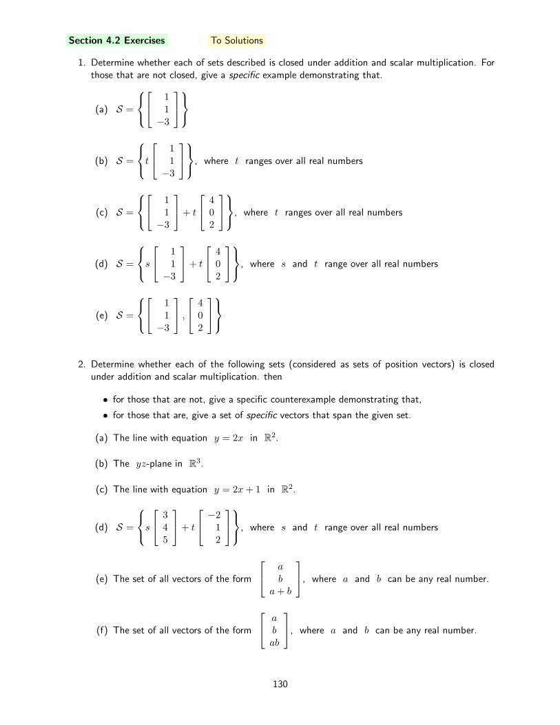
Section 4.2 Exercises To Solutions
1. Determine whether each of sets described is closed under addition and scalar multiplication. Forthose that are not closed, give a specific example demonstrating that.
(a) S =
11−3
(b) S =
t
11−3
, where t ranges over all real numbers
(c) S =
11−3
+ t
402
, where t ranges over all real numbers
(d) S =
s
11−3
+ t
402
, where s and t range over all real numbers
(e) S =
11−3
,
402
2. Determine whether each of the following sets (considered as sets of position vectors) is closedunder addition and scalar multiplication. then
• for those that are not, give a specific counterexample demonstrating that,
• for those that are, give a set of specific vectors that span the given set.
(a) The line with equation y = 2x in R2.
(b) The yz-plane in R3.
(c) The line with equation y = 2x+ 1 in R2.
(d) S =
s
345
+ t
−212
, where s and t range over all real numbers
(e) The set of all vectors of the form
a
b
a+ b
, where a and b can be any real number.
(f) The set of all vectors of the form
a
b
ab
, where a and b can be any real number.
130

4.3 Vector Spaces and Subspaces
Performance Criterion:
4. (d) Determine whether a subset of Rn is a subspace. If so, prove it; if not,
give an appropriate counterexample.
Vector Spaces
The term “space” in math simply means a set of objects with some additional special properties.There are metric spaces, function spaces, topological spaces, Banach spaces, and more. The vectorsthat we have been dealing with make up the vector spaces called R
2, R3 and, for larger values,
Rn. In general, a vector space is simply a collection of objects called vectors, a set of scalars, and two
operations that satisfy certain properties.
Definition 4.3.1: Vector Space
A vector space is a set V of objects called vectors and a set of scalars (usually thereal numbers R), with the operations of vector addition and scalar multiplication,for which the following properties hold for all
u,
v,
w in V and scalars c andd.
1.
u +
v is in V
2.
u +
v =
v +
u
3. (
u +
v)+
w =
u +(
v +
w)
4. There exists a vector
0 in V such that
u +
0 =
u. This vector is calledthe zero vector.
5. For every
u in V there exists a vector −
u in V such that
u +(−
u) =
0.
6. c
u is in V .
7. c (
u +
v) = c
u + c
v
8. (c+ d)
u = c
u + d
u
9. c (d
u) = (cd)
u
10. 1
u =
u
Note that items 1 and 6 of the above definition say that a vector space is closed under addition andscalar multiplication.
When working with vector spaces, we will be very interested in certain subsets of those vector spacesthat are the span of a set of vectors. As you proceed, recall Example 4.2(b), where we showed that thespan of a set of vectors is closed under addition and scalar multiplication.
131

Subspaces of Vector Spaces
As you should know by now, the two main operations with vectors are multiplication by scalarsand addition of vectors. (Note that these two combined give us linear combinations, the foundation ofalmost everything we’ve done.) A given vector space can have all sorts of subsets; consider the followingsubsets of R
2.
• The set S1 consisting of the first quadrant and the nonnegative parts of the two axes, or all
vectors of the form
[
x1x2
]
such that x1 ≥ 0 and x2 ≥ 0.
• The set S2 consisting of the line containing the vector
[
32
]
. Algebraically this is all vectors
of the form t
[
32
]
where t ranges over all real numbers.
• The set S3 consisting of the first and third quadrants and both axes. This can be described as
the set of all vectors
[
x1x2
]
with x1x2 ≥ 0.
Our current concern is whether these subsets of R2 are closed under addition and scalar multiplication.
With a bit of thought you should see that S1 is closed under addition, but not scalar multiplicationwhen the scalar is negative:
u
v
u +
vS1
w
c
wc < 0
S1
In some sense we can solve the problem of not being closed under scalar multiplication by including thethird quadrant as well to get S3, but then the set isn’t closed under addition:
w
c
wc < 0
S3
S3
u
v
u +
v
S3
S3
Finally, the set S2 is closed under both addition and scalar multiplication. That is a bit messy to show
with a diagram, but consider the following. S2 is the span of the single vector
[
32
]
, and we showed
in the last section that the span of any set of vectors is closed under addition and scalar multiplication.It turns out that when working with vector spaces the only subsets of any real interest are the ones
that are closed under both addition and scalar multiplication. We give such subsets a name:
132

Definition 4.3.2: Subspace of Rn
A subset S of Rn is called a subspace of R
n if for every scalar c and anyvectors
u and
v in S, c
u and
u +
v are also in S. That is, S is closedunder scalar multiplication and addition.
You will be asked whether certain subsets of R2, R
3 or Rn are subspaces, and it is your job to
back your answers up with some reasoning. This is done as follows:
• When a subset IS a subspace a general proof is required. That is, we must show that the set isclosed under scalar multiplication and addition, for ALL scalars and ALL vectors. We may haveto do this outright, but if it is clear that the set of vectors is the span of some set of vectors, thenwe know from the argument presented in Example 4.2(b) that the set is closed under additionand scalar multiplication, so it is a subspace.
• When a subset IS NOT a subspace, we demonstrate that fact with a SPECIFIC example. Such anexample is called a counterexample. Notice that all we need to do to show that a subset is nota subspace is to show that either it is not closed under scalar multiplication OR it is not closedunder scalar multiplication vector addition. If either is the case, then the set in question is not asubspace. Even if both are the case, we need only show one.
The following examples illustrate these things.
⋄ Example 4.3(a): Show that the set S1 consisting of all vectors of the form
[
x1x2
]
such
that x1 ≥ 0 and x2 ≥ 0 is not a subspace of R2.
Solution: As mentioned before, this set is not closed under multiplication by negative scalars, so
we just need to give a specific example of this. Let
u=
[
35
]
and c = −2. Clearly
u is in
S1 and c
u = (−2)[
35
]
=
[
−6−10
]
, which is not in S1. Therefore S1 is not closed under
scalar multiplication so it is not a subspace of R2.
⋄ Example 4.3(b): Show that the set S2 consisting of all vectors of the form t
312
, where
t ranges over all real numbers, is a subspace of R3.
Solution: Let c be any scalar and let
u = s
312
and
v = t
312
. Then
u and
v are
both in S2 and
c
u = c
s
312
= (cs)
312
and
u +
v = s
312
+ t
312
= (s+ t)
312
.
Because cs and s+ t are scalars, we can see that both c
u and
u +
v are in S2, so S2 isa subspace of R
3.
133

This last example demonstrates the general method for showing that a set of vectors is closed underaddition and scalar multiplication. That said, the given subspace could have been shown to be a subspace
by simply observing that it is the span of the set consisting of the single vector
312
. From Theorem
4.2.2 we know that the span of any set of vectors is closed under addition and scalar multiplication, soa span of a set is a subspace. Therefore the set described in the above example is a subspace of R
2.Let’s formalize all that:
Corollary 4.3.3: The Span of a Set is a Subspace
The span of a set S in Rn is a subspace of R
n.
In Example 4.3(d) you will see how we can use the above to prove that a set is a subspace. First welook at another example.
⋄ Example 4.3(c): Determine whether the subset S of R3 consisting of all vectors of the form
x =
25−1
+ t
4−13
is a subspace. If it is, prove it. If it is not, provide a counterexample.
u
l
Solution: We recognize this as a line in R3 passing through the point
(2, 5,−1), and it is not hard to show that the line does not pass throughthe origin. Remember that what we mean by the line is really all po-sition vectors (so with tails at the origin) whose tips are on the line.Considering a similar situation in R
2, we see that
u is such a vectorfor the line l shown. It should be clear that if we multiply
u by anyscalar other than one, the resulting vector’s tip will not lie on the line.Thus we would guess that the set S, even though it is in R
3, is probablynot closed under scalar multiplication.
Now let’s prove that it isn’t. To do this we first let
u =
25−1
+ 1
4−13
=
642
, which
is in S. Let c = 2, so 2
u =
1284
. We need to show that this vector is not in S. If it
were, there would have to be a scalar t such that
1284
=
25−1
+ t
4−13
. Subtracting
25−1
from both sides we get
1035
= t
4−13
. We can see that the value of t that
would be needed to give the correct second component would be −3, but this would result in a
third component of −9, which is not correct. Thus there is no such t and the vector
1284
is
not in S. Thus S is not closed under scalar multiplication, so it is not a subspace of R3.
134

This example may seem to contradict Corollary 4.3.3. The reason it does not is because the vectors ofthe
form
25−1
+ t
4−13
do not include ALL linear combinations of the vectors
25−1
and
4−13
.
We should compare the results of Examples 4.3(b) and 4.3(c). Note that both are lines in theirrespective R
n’s, but the line in 4.3(b) passes through the origin, and the one in 4.3(c) does not. It isno coincidence that the set in 4.3(b) is a subspace and the set in 4.3(c) is not. If a set S is a subspace,being closed under scalar multiplication means that zero times any vector in the subspace must also bein the subspace. But zero times a vector is the zero vector 0. Therefore
Theorem 4.3.4: Subspaces Contain the Zero Vector
If a subset S of Rn is a subspace, then the zero vector of R
n is in S.
This type of a statement is called a conditional statement. Related to any conditional statement aretwo other statements called the converse and contrapositive of the conditional statement. In this casewe have
• Converse: If the zero vector is in a subset S of Rn, then S is a subspace.
• Contrapositive: If the zero vector is not in a subset S of Rn, then S is not a subspace.
When a conditional statement is true, its converse may or may not be true. In this case the converseis not true. This is easily seen in Example 4.3(a), where the set contains the zero vector but is not asubspace. However, when a conditional statement is true, its contrapositive is true as well. Thereforethe second statement above is the most useful of the three statements, since it gives us a quick way torule out a set as a subspace. Let’s recognize it formally.
Corollary 4.3.5: Test For Not a Subspace
If a subset S of Rn does not the zero vector of R
n, then it is not a subspaceof R
n.
In Example 4.3(c) this would have saved us the trouble of providing a counterexample, although we’dstill need to convincingly show that the zero vector is not in the set.
⋄ Example 4.3(d): Determine whether the set of all vectors of the form
x =
a
a+ b
b
a− b
, for
some real numbers a and b, is a subspace of R4.
135

Solution: We first note that a vector
x of the given form will be the zero vector if a = b = 0.We cannot then use the above result to rule out the possibility that the given set is a subspace,but neither do we yet know it IS a subspace. But we observe that
x =
a
a+ b
b
a− b
=
a
a
0a
+
0b
b
−b
= a
1101
+ b
011−1
.
Thus, by Corollary 4.3.3, the set of vectors under consideration is the span of S =
1101
,
011−1
,
so it is a subspace of R4.
We conclude this section with an example that gives us the “largest” and “smallest” subspaces ofRn.
⋄ Example 4.3(e): Of course a scalar times any vector in Rn is also in R
n, and the sum ofany two vectors in R
n is in Rn, so R
n is a subspace of itself. Also, the zero vector by itselfis a subspace of R
n as well, often called the trivial subspace.
At this point we have seen a variety of subspaces, and some sets that are not subspaces as well.Now supose that we have two vectors in R
3 that are not scalar multiples of each other. We knowthat the span of the two vectors is a plane through the origin in R
3. Note that we could impose acoordinate system on any plane to make it essentially R
2, so we can think of this particular variety ofsubspace as just being a copy of R
2 “sitting inside” R3. This illustrates what is in fact a general
principle: any subspace of Rn is essentially a copy of R
m, for some m ≤ n, sitting inside Rn with
its origin at the origin of Rn. More formally we have the following:
Subspaces of Rn
• The only non-trivial subspaces of R2 are lines through the origin and all of
R2.
• The only non-trivial subspaces of R3 are lines through the origin, planes
through the origin, and all of R3.
• The only non-trivial subspaces of Rn are hyperplanes (including lines) through
the origin and all of Rn.
136

Section 4.3 Exercises To Solutions
1. For each of the following subsets of R3, think of each point as a position vector; each set thenbecomes a set of vectors rather than points. For each,
• determine whether the set is a subspace and
• if it is NOT a subspace, give a reason why it isn’t by doing one of the following:
⋄ stating that the set does not contain the zero vector
⋄ giving a vector that is in the set and a scalar multiple that isn’t (show that it isn’t)
⋄ giving two vectors that in the set and showing that their sum is not in the set
(a) All points on the horizontal plane at z = 3.
(b) All points on the xz-plane.
(c) All points on the line containing
u = [−3, 1, 4].(d) All points on the lines containing
u = [−3, 1, 4] and
v = [5, 0, 2].
(e) All points for which x ≥ 0, y ≥ 0 and z ≥ 0.
(f) All points
x given by
x =
w + s
u + t
v, where
w = [1, 1, 1] and
u and
v are as in(d).
(g) All points
x given by
x = s
u + t
v, where
u and
v are as in (d).
(h) The vector 0.
(i) All of R3.
2. Consider the vectors
u =
8−24
,
v =
701
and
w =
−164−8
.
(a) Is the set of all vectors
x =
u + t
v, where t ranges over all real numbers, a subspaceof R
3? If not, tell why not.
(b) Is the set of all vectors
x =
u + t
w, where t ranges over all real numbers, a subspaceof R
3? If not, tell why not.
137

4.4 Column Space and Null Space of a Matrix
Performance Criteria:
4. (e) Determine whether a vector is in the column space or null space of amatrix, based only on the definitions of those spaces.
In this section we will define two important subspaces associated with a matrix A, its columnspace and its null space.
Definition 4.4.1: Column Space of a Matrix
The column space of an m× n matrix A is the span of the columns of A. Itis a subspace of R
m and we denote it by col(A).
⋄ Example 4.4(a): Determine whether
u =
338
and
v =
−251
are in the column space
of A =
2 5 1−1 −7 −53 4 −2
.
Solution: We need to solve the two vector equations of the form
c1
2−13
+ c2
5−74
+ c3
1−5−2
=
b, (1)
with
b first being
u, then
v. The respective reduced row-echelon forms of the augmentedmatrices corresponding to the two systems are
1 0 −2 40 1 1 −10 0 0 0
and
1 0 −2 00 1 1 00 0 0 1
Therefore we can find scalars c1, c2 and c3 for which (1) holds when
b =
u, but not when
b =
v. From this we deduce that
u is in col(A), but
v is not.
Recall that the system A
x =
b of m linear equations in n unknowns can be written in linearcombination form:
x1
a11
a21
...
am1
+ x2
a12
a22
...
am2
+ · · ·+ xn
a1n
a2n
...
amn
=
b1
b2
...
bn
138

Note that the left side of this equation is simply a linear combination of the columns of A, with thescalars being the components of
x. The system will have a solution if, and only if,
b can be writtenas a linear combination of the columns of A. Stated another way, we have the following:
Theorem 4.4.2: A system A
x =
b has a solution (meaning at least one
solution) if, and only if,
b is in the column space of A.
Let’s consider now only the case where m = n, so we have n linear equations in n unknowns. Wehave the following facts:
• If col(A) is all of Rn , then A
x =
b will have a solution for any vector
b. What’s more,the solution will be unique.
• If col(A) is a proper subspace of Rn (that is, it is not all of R
n), then the equation
A
x =
b will have a solution if, and only if,
b is in col(A). If
b is in col(A) the systemwill have infinitely many solutions.
Next we define the null space of a matrix.
Definition 4.4.3: Null Space of a Matrix
The null space of an m× n matrix A is the set of all solutions to A
x= 0. Itis a subspace of R
n and is denoted by null(A).
⋄ Example 4.4(b): Determine whether
u =
104
and
v =
2−11
are in the null space
of A =
2 5 1−1 −7 −53 4 −2
.
Solution: A vector
x is in the null space of a matrix A if A
x = 0. We see that
A
u =
2 5 1−1 −7 −53 4 −2
104
=
6−2111
and A
v =
2 5 1−1 −7 −53 4 −2
2−11
=
000
so
v is in null(A) and
u is not.
Again considering the case where m = n, we have the following fact about the null space:
• If null(A) is just the zero vector, A is invertible and A
x =
b has a unique solution for any
vector
b.
139

We conclude by pointing out the important fact that for an m× n matrix A, the null space ofA is a subspace of R
n and the column space of A is a subspace of Rm.
Section 4.4 Exercises To Solutions
1. For each of the following, a matrix A and a vector
u are given. in each case, determine whether
u is in the column space of A. You should be able to do all of these by inspection, meaningwithout doing any computations other than some mental arithmetic.
(a) A =
1 0 0
0 1 0
0 0 1
,
u =
2−13
(b) A =
1 0 1
0 1 1
0 0 0
,
u =
2−13
(c) A =
[
2 −3−5 1
]
,
u =
[
47
]
(d) A =
[
2 −3−4 6
]
,
u =
[
8−16
]
(e) A =
[
2 −3−4 6
]
,
u =
[
5−2
]
(f) A =
1 0 0
0 1 0
0 0 1
,
u =
140
2. Let A =
1 1 0
2 3 −2−1 −4 6
,
u1 =
29
−17
,
u2 =
3152
.
(a) Remember that the column space of A is simply the set of all vectors that are linearcombinations of the columns of A. Determine whether the vector
u1 is in the columnspace of A by determining whether
u1 is a linear combination of the columns of A. Givethe vector equation that you are trying to solve, and your row reduced augmented matrix.Be sure to tell whether
u1 is in the column space of A or not! Do this with abrief sentence.
(b) If
u1 IS in the column space of A, give a specific linear combination of the columns ofA that equals
u1.
(c) Repeat parts (a) and (b) for the vector
u2.
3. Let A =
1 1 0
2 3 −2−1 −4 6
,
v1 =
8−8−4
,
v2 =
50−7
. The null space of A is just
all the vectors
x for which A
x = 0, and it is denoted by null(A). This means that to checkto see if a vector
x is in the null space we need only to compute A
x and see if it is the zerovector. Use this method to determine whether either of the vectors
v1 and
v2 is in null(A).Give your answer as a brief sentence.
140

4. Let A =
3 −2 1
1 3 4
−1 −4 −5
.
(a) Is
u1 =
5−23
in col(A)? Justify your answer.
(b) Is
u2 =
111
in col(A)? Justify your answer.
(c) Does the system A
x =
b have a solution for all vectors
b in R3? Explain.
(d) Give a non-zero vector
v1 that is in the null space of A.
(e) Is A invertible? Explain.
5. (a) Give a 2× 2 matrix A with no zero entries whose column space is all of R2.
(b) Give a 2× 2 matrix B with no zero entries whose column space is NOT all of R2.
(c) For either of your matrices A and B from parts (a) and (b) that you can, find a nonzerovector in the null space of the matrix.
6. For non-square matrices, the column space and null space contain vectors in different Rns.
Consider the matrix
A =
[
2 −3 1
−5 1 4
]
.
(a) Vectors in the column space are in what Rn?
(b) Vectors in the null space are in what Rn?
(c) Can you find a vector in the Rn of the column space that IS NOT in the column space of
A? If so, give one. If not, explain.
(d) Can you find a nonzero vector in the Rn of the null space that IS in the null space of A?
If so, give one. If not, explain.
141

4.5 Least Squares Solutions to Inconsistent Systems
Performance Criterion:
4. (f) Find the least-squares approximation to the solution of an inconsistentsystem of equations. Solve a problem using least-squares approximation.
(g) Give the least squares error and least squares error vector for a leastsquares approximation to a solution to a system of equations.
Let’s begin with a motivating example.
⋄ Example 4.5(a): Find the equation of the line containing the five points with coordinates
(1.2, 3.7) (2.5, 4.1) (3.2, 4.7) (4.3, 5.2) (5.1, 5.9).
Solution: We substitute each pair of points into the equation y = mx+ b of a line to get thesystem shown below and to the left.
1.2m+ b = 3.72.5m+ b = 4.13.2m+ b = 4.74.3m+ b = 5.25.1m+ b = 5.9
=⇒
1.2 1 3.72.5 1 4.13.2 1 4.74.3 1 5.25.1 1 5.9
rref=⇒
1 0 00 1 00 0 10 0 00 0 0
4
4x
y
When then row-reduce the augmented matrix for this system in order to solve the system. Whenwe do this, we get the last matrix above as our row-reduced matrix, indicating that the systemhas no solution. The five points are plotted above and to the right, and we can see that they arenot on a line, which is why we were not able to solve the system. You may remember that such asystem is sometimes referred to as overdetermined, meaning that there is too much informationto allow a solution to the system. We conclude that there is no line through all of the givenpoints.
Recall that an inconsistent system is one for which there is no solution. Often we wish to solve aninconsistent system A
x =
b, and it is just not acceptable to have no solution. In those cases wecan find some vector (whose components are the values we are trying to find when attempting to solvethe system) that is “closer to being a solution” than all other vectors. The theory behind this processis part of the second term of this course, but we now have enough knowledge to find such a vector in a“cookbook” manner.
Suppose that we have a system of equations A
x =
b. Pause for a moment to reflect on what weknow and what we are trying to find when solving such a system: We have a system of linear equations,and the entries of A are the coefficients of all the equations. The vector
b is the vector whosecomponents are the right sides of all the equations, and the vector
x is the vector whose componentsare the unknown values of the variables we are trying to find. So we know A and
b and we are tryingto find
x. If A is invertible, the solution vector
x is given by
x= A−1
b. If A is not invertiblethere will be no solution vector
x, but we can usually find a vector x (usually spoken as “ex-bar”)that comes “closest” to being a solution. Here is the formula telling us how to find that x:
142

Theorem 4.5.1: The Least Squares Theorem: Let A be an m × n matrixand let
b be in Rm. If A
x =
b has a least squares solution x, it is givenby
x = (ATA)−1AT
b
⋄ Example 4.5(b): Find the least squares solution to
1.3x1 + 0.6x2 = 3.3
4.7x1 + 1.5x2 = 13.5
3.1x1 + 5.2x2 = −0.1.
Solution: First we note that if we try to solve by row reduction we get no solution; this is anoverdetermined system because there are more equations than unknowns. The matrix A andvector
b are
A =
1.3 0.6
4.7 1.5
3.1 5.2
,
b =
3.3
13.5
−0.1
Using a calculator or MATLAB, we get
x = (ATA)−1AT
b=
[
3.5526
−2.1374
]
Example 4.5(a) is a classic example of when we want to do something like this. We have a bunchof (x, y) data pairs from some experiment, and when we graph all the pairs they describe a trend.We then want to find a simple function y = f(x) that best models that data. In some cases thatfunction might be a line, in other cases maybe it is a parabola, and in yet other cases it might be anexponential function. Let’s try to make the connection between this and linear algebra. Suppose thatwe have the data points (x1, y1), (x2, y2), ..., (xn, yn), and when we graph these points they arrangethemselves in roughly a line, as shown to the left below. We then want to find an equation of the forma + bx = y (note that this is just the familiar y = mx + b rearranged and with different letters forthe slope and y-intercept) such that a+ bxi ≈ yi for i = 1, 2, ..., n, as shown to the right below.
(x1, y1)
(x2, y2)(xn, yn)
x
y
(x1, y1)
(x2, y2)(xn, yn)
y = a+ bx
x
y
If we substitute each data pair into a+ bx = y we get a system of equations which can be thoughtof in several different ways. Remember that all the xi and yi are known values - the unknowns are
143

a and b.
a+ x1b = y1a+ x2b = y2
...a+ xnb = yn
⇐⇒
1 x11 x2...1 xn
[
a
b
]
=
y1y2...yn
⇐⇒ A
x =
b
Above we first see the system that results from putting each of the (xi, yi) pairs into the equation
a+ bx = y. After that we see the A
x =
b form of the system. We must be careful of the notationhere. A is the matrix whose columns are a vector in R
n consisting of all ones and a vector whosecomponents are the xi values. It would be logical to call this last vector
x, but instead
x is the
vector
[
a
b
]
.
b is the column vector whose components are the yi values. Our task, as described
by this interpretation, is to find a vector
x in R2 that A transforms into the vector
b in Rn.
Even if such a vector did exist, it couldn’t be given as
x = A−1
b because A is not square, socan’t be invertible. However, it is likely no such vector exists, but we CAN find the least-squares vector
x =
[
a
b
]
= (ATA)−1AT
b. When we do, its components a and b are the intercept and slope of
our line.
⋄ Example 4.5(c): Find the the least squares solution to the problem from Example 4.5(a).
Solution: Recall that we obtained the system shown below and to the left. The matrix form ofthe system is shown to the right of the system.
1.2m+ b = 3.72.5m+ b = 4.13.2m+ b = 4.74.3m+ b = 5.25.1m+ b = 5.9
=⇒
1.2 12.5 13.2 14.3 15.1 1
[
m
b
]
=
3.74.14.75.25.9
From this we determine that A =
1.2 12.5 13.2 14.3 15.1 1
,
x =
[
m
b
]
,
b =
3.74.14.75.25.9
. Note the
difference between the y-intercept b of the line we are looking for and the vector
b! We now
apply the least squares theorem to obtain x = (ATA)−1AT
b =
[
0.56
2.88
]
. The equation of
the line that is “closest” to containing the points
(1.2, 3.7) (2.5, 4.1) (3.2, 4.7) (4.3, 5.2) (5.1, 5.9).
is then y = 0.56x + 2.88.
144

To the right we see a plot of the five points and the line y =0.56x+ 2.88, showing that the line does a good job of comingclose to going through all of the points.
4
4
x
y
Theoretically, here is what is happening when use least squares to solve an inconsistent systemA
x =
b. The fact that the system A
x =
b has no solution means that
b is not in the columnspace of A. The least squares solution to A
x =
b is simply the vector x for which Ax is theclosest vector to
b that is still in col(A) - it is the projection of
b onto the column space of A.This is shown simplistically below, for the situation where the column space is a plane in R
3.
Ax
b ~ε
col(A)
To recap a bit, suppose we have a system of equations A
x =
b where there is no vector
x forwhich A
x equals
b. What the least squares approximation allows us to do is to find a vector x forwhich Ax is as “close” to
b as possible. We generally determine “closeness” of two objects by findingthe difference between them. Because both Ax and
b are both vectors with the same number ofcomponents, we can subtract them to get a vector ~ε that we will call the error vector, shown above.The least squares error is then the magnitude of this vector:
Definition 4.5.2: If x is the least-squares solution to the system A
x =
b,the least squares error vector is
~ε =
b −Ax
and the least squares error is the magnitude of ~ε.
145

⋄ Example 4.5(b): Find the least squares error vector and least squares error vector for the
solution obtained in Example 4.5(a).
Solution: The least squares error vector is
~ε =
b −Ax =
3.3
13.5
−0.1
−
1.3 0.6
4.7 1.5
3.1 5.2
[
3.5526
−2.1374
]
=
−0.03590.0089
0.0016
The least squares error is ‖~ε‖ = 0.0370.
Section 4.5 Exercises To Solutions
1. Consider the points (1, 8), (2, 7), (3, 5), (4, 2).
(a) Find the least squares approximating line y = a + bx for the points. Give the system of
equations to be solved (in any form), the matrix A and vector
b, the solution vector
x and the equation of the line.
(b) Plot the points and your line using something like Desmos. (To plot the points with Desmos,just list them exactly as they are given above.) Does the line seem to do a good job of comingclose to all of the points?
(c) Find the least squares approximating parabola y = a + bx+ cx2 for the points. Give the
system of equations to be solved (in any form), the matrix A and vector
b, the solutionvector
x and the equation of the parabola.
(d) Plot the points and your parabola using something like Desmos. Does the parabola seemto do a good job of coming close to all of the points?
2. We know that through any three non-collinear points in R3 there is exactly one plane. When
we have more than three such points there is likely not a plane containing all the points, becausethis is an overdetermined situation. But we can use least-squares to determine the plane that bestapproximates a plane through all of the points. If the plane is not vertical, its equation can bewritten
z = a+ bx+ cy,
where each of a, b and c are constants. Find the equation of the plane closest to containingthe points
(1.1, 0.2, 4.7), (4.3, 6.5, 5.0), (3.2, 5.1, 4.5), (7.4, 2.8, 13.8),
rounding each of a, b and c to the hundredth’s place.
3. Consider the system2x1 + 3x2 = 26−x1 + 5x2 = 13
.
(a) Find the least-squared solution to the system.
(b) Solve the system by some method you have used for consistent systems (those that have“ordinary” solutions).
(c) How do your solutions from (a) and (b) compare?
146

4.6 Linear Independence
Performance Criterion:
4. (h) Determine whether a set
v1,
v2, ...,
vk of vectors is a linearly independentor linearly dependent. If the vectors are linearly dependent, (1) give anon-trivial linear combination of them that equals the zero vector, (2)give any one as a linear combination of the others, when possible.
In Exercise 6 of Section 4.1 we considered several sets of vectors in R3, including the sets
S1 =
100
,
010
, S2 =
100
,
010
,
001
,
S5 =
100
,
010
,
001
,
111
It should be clear that set S1 does not span R3, and that any vector
a
b
c
in R3 is in the
span of S2:
a
b
c
= a
100
+ b
010
+ c
001
.
Because S2 spans R3, including the additional vector as done in S5 does not increase the span,
but of course it doesn’t decrease it either. Therefore we can construct any vector in R3 as a linear
combination of iether vectors from S2 or vectors from S5. We will find that S5 is undesirable forgetting vectors in R
3 for the following reason:
123
= 1
100
+ 2
010
+ 3
001
+ 0
111
and
123
= 0
100
+ 1
010
+ 2
001
+ 1
111
This shows that the vector
123
can be constructed as a linear combination of vectors in S5
in more than one way. In fact, there are infinitely many different linear combinations of the vectors inS5 that equal any vector in R
3. On the other hand, it should be clear that, given any vector in R3,
there is only one way to obtain that vector as a linear combination of vectors in S2. So even thoughboth sets S2 and S5 span R
3, We will find that a set like S2, with enough vectors to span, butnot “too many,” is more desirable.
Let’s take a look at what is going on from a different perspective. Suppose that we are trying to
create a set S of vectors that spans R3. We might begin with one vector, say
u1 =
−312
, in S.
147

We know by now that the span of this single vector is all scalar multiples of it, which is a line in R3.
If we wish to increase the span, we would add another vector to S. If we were to add a vector like
6−2−4
to S, we would not increase the span, because this new vector is a scalar multiple of
u1, so
it is on the line we already have and would contribute nothing new to the span of S. To increase thespan, we need to add to S a second vector
u2 that is not a scalar multiple of the vector
u1 that
we already have. It should be clear that the vector
u2 =
111
is not a scalar multiple of
u1, so
adding it to S would increase it’s span.The span of S = u1,
u2 is a plane. When S included only a single vector, it was relatively easyto determine a second vector that, when added to S, would increase it’s span. Now we wish to adda third vector to S to further increase its span. Geometrically it is clear that we need a third vectorthat is not in the plane spanned by u1,
u2. Probabilistically, just about any vector in R3 would
do, but what we would like to do here is create an algebraic condition that needs to be met by a thirdvector so that adding it to S will increase the span of S.
Let’s begin with what we DON’T want: we don’t want the new vector to be in the plane spannedby u1,
u2. Now every vector
v in that plane is of the form
v = c1
u1 +c2
u2 for some scalarsc1 and c2. We say the vector
v created this way is “dependent” on
u1 and
u2, and that iswhat causes it to not be helpful in increasing the span of a set that already contains those two vectors.Assuming that neither of c1 and c2 is zero, we could also write
u1 =c2
c1
u2 −1
c1
v and
u2 =c1
c2
u1 −1
c2
v,
showing that
u1 is “dependent” on
u2 and
v, and
u2 is “dependent” on
u1 and
v. Sowhatever “dependent” means (we’ll define it more formally soon), all three vectors are dependent oneach other. We can create another equation that is equivalent to all three of the ones given so far, andthat does not “favor” any particular one of the three vectors:
c1
u1 +c2
u2 +c3
v=
0,
where c3 = −1.Of course, if we want a third vector
u3 to add to u1,
u2 to increase its span, we would notwant to choose
u3 =
v; instead we would want a third vector that is “independent” of the two wealready have. Based on what we have been doing, we would suspect that we would want
c1
u1 +c2
u2 +c3
u3 6=
0 . (1)
Of course even if
u3 was not in the plane spanned by
u1 and
u2, (1) would be true if c1 = c2 =c3 = 0, but we want that to be the only choice of scalars that makes (1) true.
We now make the following definition, based on our discussion:
Definition 4.6.1: Linear Dependence and Independence
A set S = u1,
u2, ...,
uk of vectors is linearly dependent if there exist scalarsc1, c2, ..., ck, not all equal to zero such that
c1
u1 + c2
u2 + · · ·+ ck
uk =0. (2)
If (2) only holds for c1 = c2 = · · · = ck = 0 the set S is linearly independent.
148

We can state linear dependence (independence) in either of two ways. We can say that the set is linearlydependent, or the vectors are linearly dependent. Either way is acceptable. Often we will get lazy andleave off the “linear” of linear dependence or linear independence. This does no harm, as there is noother kind of dependence/independence that we will be interested in.
⋄ Example 4.6(a): Determine whether the vectors
−1−7311
,
1−325
and
7−143
are
linearly dependent, or linearly independent. If they are dependent, give a non-trivial linear com-bination of them that equals the zero vector. (Non-trivial means that not all of the scalars arezero!)
Solution: To make such a determination we always begin with the vector equation from thedefinition:
c1
−1−7311
+ c2
1−325
+ c3
7−143
=
0000
(3)
We recognize this as the linear combination form of a system of equations that has the augmentedmatrix shown below and to the left, which reduces to the matrix shown below and to the right.
−1 1 7 0−7 −3 −1 03 2 4 0
11 5 3 0
1 0 −2 00 1 5 00 0 0 00 0 0 0
From this we see that there are infinitely many solutions, so there are certainly values of c1,c2 and c3, not all zero, that make (4) true, so the set of vectors is linearly dependent. To finda non-trivial linear combination of the vectors that equals the zero vector we let the free variablec3 be any value other than zero. (You should try letting it be zero to see what happens.) If wetake c3 to be one, then c2 = −5 and c1 = 2. Then
2
−1−73
11
− 5
1−325
+
7−143
=
−2−14
622
+
−515−10−25
+
7−143
=
0000
⋄ Example 4.6(b): Determine whether the vectors
−3−12
,
470
and
−25−1
are
linearly dependent, or linearly independent. If they are dependent, give a non-trivial linear com-bination of them that equals the zero vector. (Non-trivial means that not all of the scalars arezero!)
Solution: To make such a determination we always begin with the vector equation from thedefinition:
c1
3−12
+ c2
470
+ c3
−25−1
=
000
149

We recognize this as the linear combination form of a system of equations that has the augmentedmatrix shown below and to the left, which reduces to the matrix shown below and to the right.
3 4 −2 0−1 7 5 02 0 −1 0
1 0 0 00 1 0 00 0 1 0
We see that the only solution to the system is c1 = c2 = c3 = 0, so the vectors are linearlyindependent.
A comment is in order at this point. The system c1
u1 +c2
u2 + · · ·+ ck
uk= 0 is homogeneous,so it will always have at least the zero vector as a solution. It is precisely when the only solution is thezero vector that the vectors are linearly independent.
Now suppose we have a set u1,
u2, ...,
uk of linearly dependent vectors in Rn. By definitions,
there are scalars c1, c2, ..., ck , not all equal to zero, such that
c1
u1 + c2
u2 + · · ·+ ck
uk =
0
Let cj , for some j between 1 and k, be one of the non-zero scalars. (By definition there has tobe at least one such scalar.) Then we can do the following:
c1
u1 + c2
u2 + · · ·+ cj
uj + · · ·+ ck
uk =
0
cj
uj = − c1
u1 − c2
u2 − · · · − ck
uk
uj = −c1
cj
u1 −c2
cj
u2 − · · · −ck
cj
uk
uj = d1
u1 + d2
u2 + · · ·+ dk
uk
This, along with the fact that the above computation can be reversed, gives us the following:
Theorem 4.6.2: A set S = u1,
u2, ...,
uk is linearly dependent if, and only if,at least one of these vectors can be written as a linear combination of the remainingvectors.
The importance of this, which we’ll reiterate again later, is that if we have a set of linearly dependentvectors with a certain span, we can eliminate at least one vector from our original set without reducingthe span of the set. If, on the other hand, we have a set of linearly independent vectors, eliminatingany vector from the set will reduce the span of the set.
⋄ Example 4.6(c): In Example 4.6(a) we determined that the vectors
−1−7311
,
1−325
and
7−143
are linearly dependent. Give one of them as a linear combination of the others.
150

Solution: In Example 4.6(a) we found that the vector equation
c1
−1−7311
+ c2
1−325
+ c3
7−143
=
0000
had infinitely many solutions, one of which was
2
−1−7311
− 5
1−325
+
7−143
=
0000
(4)
We can easily solve that equation for the third vector to get
7−143
= −2
−1−73
11
+ 5
1−325
Note that we could also have solved (4) for either the first or second vectors. Solving for the firstwould give us
−1−7311
=5
2
1−325
− 1
2
7−143
,
and we could solve for the second in a similar manner.
⋄ Example 4.6(d): Determine whether the vectors
4−13
,
1−31
and
322
are linearly
dependent.
Solution: We can easily observe that
1−31
+
322
=
4−13
, so the first vector
is a linear combination of the other two. By Theorem 4.6.2, the three vectors are linearly depen-dent.
We now consider three vectors
u1,
u2 and
u3 in R2 whose sum
is not the zero vector, and for which no two of the vectors are parallel.I have arranged these to show the tip-to-tail sum in the top diagram tothe right; clearly their sum is not the zero vector.
u1
u2
u3
u1 +
u2 +
u3x
y
151

At this point if we were to multiply
u2 by some scalar c2 less thanone we could shorten it to the point that after adding it to
u1 the tipof c2
u2 would be in such a position as to line up
u3 with the origin.This is shown in the bottom diagram to the right.
u1
c2
u2
u3
u1 +c2
u2 +
u3
u1
c2
u2
c3
u3
u1 +c2
u2 +c3
u3= 0
Finally, we could then multiply
u3 by a scalar c3 greater than oneto lengthen it to the point of putting its tip at the origin. We wouldthen have
u1 +c2
u2 +c3
u3= 0. You should play around with a fewpictures to convince yourself that this can always be done with threevectors in R
2, as long as none of them are parallel (scalar multiplesof each other). This shows us that any three vectors in R
2 are alwayslinearly dependent. In fact, we can say even more:
Theorem 4.6.3: Any set of more than n vectors in Rn must be linearly
dependent.
⋄ Example 4.6(e): Determine whether the vectors
[
12
]
,
[
3−1
]
and
[
55
]
.
Solution: This is a set of three vectors in R2 (Rn with n = 2), so by the above theorem they
must be dependent.
Note that Theorem 4.6.3 doesn’t tell us that a set of n or fewer vectors in Rn must be linearly
independent!
⋄ Example 4.6(f): Determine whether the vectors
123
and
246
are independent.
Solution: Note that this is a set of two vectors in Rn with n = 3. The above theorem is
therefore not helpful. However, we can see that the second vector is a linear combination of thefirst (two times it), so by Theorem 4.6.2 the vectors are linearly dependent.
152

Section 4.6 Exercises To Solutions
1. Determine whether each set of vectors is linearly independent or linearly dependent without ap-plying the definition. That is, use Theorems 4.6.2 and 4.6.3. In each case, explain your reasoning.
(a) S =
2−15
,
170
, (b) S =
[
41
]
(c) S =
100
,
101
,
001
(d) S =
[
46
]
,
[
69
]
(e) S =
111
,
123
,
201
,
077
2. Consider the vectors
u1 =
−594
,
u2 =
506
, and
u3 =
59
16
.
(a) Give the VECTOR equation that we must consider in order to determine whether the threevectors are linearly independent.
(b) Your equation has one solution for sure. What is it? What does it mean (in terms of lineardependence or independence) if that is the ONLY solution?
(c) Write your equation from (a) as a system of linear equations. Then give the augmentedmatrix for the system.
(d) Does the system have more solutions than the one you gave in (b)? If so, find one of them.(By “one” I mean one ordered triple of three numbers.)
(e) Find each of the three vectors as a linear combination of the other two.
3. Show that the vectors
u =
−134
,
v =
51−6
and
w =
−449
are linearly
dependent. Then give one of the vectors as a linear combination of the others.
4. For the following, use the vectors
v1 =
13−1
,
v2 =
1−24
,
v3 =
14−2
.
(a) Determine whether
u =
401
and
w =
05−5
are in span(
v1,
v2,
v3).
153

(b) Show that the vectors
v1,
v2 and
v3 are linearly dependent by the definition of linearlydependent. In other words, produce scalars c1, c2 and c3 and demonstrate that they andthe vectors satisfy the equation given in the definition.
(c) Since the vectors are linearly dependent, at least one the vectors can be expressed as a linearcombination of the other two. Express
v1 as a linear combination of
v2 and
v3.
154

4.7 Bases of Subspaces, Dimension
Performance Criterion:
4. (i) Determine whether a given set of vectors is a basis for a given subspace.Give a basis and the dimension of a subspace.
We have seen that the span of any set of vectors in Rn is a subspace of R
n. In a sense, thevectors whose span is being considered are the “building blocks” of the subspace. That is, every vectorin the subspace is some linear combination of those vectors. Now, recall that if a set of vectors is linearlydependent, one of the vectors can be represented as a linear combination of the others. So if we areconsidering the span of a set of dependent vectors, we can throw out the one that can be obtained asa linear combination without affecting the span of the set of vectors.
So given a subspace, it is desirable to find what we might call a minimal spanning set, the smallestset of vectors whose linear combinations gives the entire subspace. Such a set is called a basis.
Definition 4.7.1: Basis of a Subspace
For a subspace S, a basis is a set B of vectors such that
• the span of B is S,
• the vectors in B are linearly independent
The plural of basis is bases (pronounced “base-eez”). With a little thought, you should believe thatevery subspace has infinitely many bases. (This is a tiny lie - the trivial subspace consisting of just thezero has no basis vectors, which is a funny consequence of logic.)
⋄ Example 4.7(a): Is the set B =
100
,
010
,
001
a basis for R3?
Solution: Clearly for any vector
a
b
c
in R3 we have
a
b
c
= a
100
+b
010
+c
001
,
so the
span of B is all of R3. The augmented matrix for testing for linear independence is simply the
identity augmented with the zero vector, giving only the solution where all the scalars are zero,so the vectors are linearly independent. Therefore the set B is a basis for R
3.
The basis just given is called the standard basis for R3, and its vectors are often denoted by
e1,
e2 and
e3. There is a standard basis for every Rn, and
e1 is always the vector whose firstcomponent is one and all others are zero,
e2 is the vector whose second component is one and allothers are zero, and so on.
155

⋄ Example 4.7(b): Let S1 =
−315
,
27−4
. In the previous section we saw that
span(S1) is a subspace of R3. Is S1 a basis for span(S1)?
Solution: Clearly S1 meets the first condition for being a basis and, since we can see that neitherof these vectors is a scalar multiple of the other, they are linearly independent. Therefore they area basis for span(S1).
⋄ Example 4.7(c): Let S2 =
−315
,
27−4
,
56−9
. Span(S2) is a subspace
of R3; is S2 a basis for span(S2)?
Solution: Once again this set meets the first condition of being a subspace. We can also see that
(−1)
−315
+
27−4
=
56−9
, so the set S2 is linearly dependent. Therefore it is NOT a
basis for span(S).
⋄ Example 4.7(d): The yz-plane in R3 is a subspace. Give a basis for this subspace.
Solution: We know that a set of two linearly independent vectors will span a plane, so we simplyneed two vectors in the yz-plane that are not scalar multiples of each other. The simplest choices
are the two vectors
e2=
010
and
e3=
001
, so they are a basis for the yz-plane.
Considering this last example, it is not hard to show that the set
010
,
011
is also a
basis for the yz-plane, and there are many other sets that are bases for that plane as well. All of thosesets will contain two vectors, illustrating the fact that every basis of a subspace has the same numberof vectors. This allows us to make the following definition:
Definition 4.7.2: Dimension of a Subspace
The dimension of a subspace is the number of elements in a basis for that subspace.
Looking back at Examples 4.7(a), (b) and (d), we then see that R3 has dimension three, and
span(S1) has dimension two, and the yz-plane in R3 has dimension two.
Although its importance may not be obvious to you at this point, here’s why we care about a basisrather than any set that spans a subspace:
156

Theorem 4.7.3: Any vector in a subspace S with basis B is represented by one,and only one, linear combination of vectors in B.
⋄ Example 4.7(e): In Example 4.7(d) we determined that the set of all vectors of the form
x=
a
a+ b
b
a− b
, for some real numbers a and b, is a subspace of R4. Give a basis for that
subspace.
Solution: The key computation in Example 4.7(d) was
x=
a
a+ b
b
a− b
=
a
a
0a
+
0b
b
−b
= a
1101
+ b
011−1
.
The set of vectors under consideration is spanned by S =
1101
,
011−1
, and we can see
that those two vectors are linearly independent (because they aren’t scalar multiples of each other,which is sufficient for independence when considering just two vectors). Therefore they form abasis for the subspace of vectors of the given form.
Section 4.7 Exercises To Solutions
1. Which of the following is a basis for R2? For those that aren’t, tell why not.
S1 =
[
12
]
,
[
31
]
,
[
11
]
S2 =
[
12
]
,
[
31
]
S3 =
[
12
]
2. Which if the following is a basis for R3? For those that aren’t, tell why not.
S1 =
100
,
110
,
111
S2 =
101
,
110
,
011
S3 =
123
,
111
,
147
S4 =
123
,
111
,
102
3. Which of the following is a basis for the line in R2 containing the vector
[
31
]
? For those
that aren’t, tell why not.
S1 =
[
31
]
,
[
62
]
S2 =
[
62
]
S3 =
[
12
]
157

4. Which of the following is a basis for the yz-plane in R3? For those that aren’t, tell why not.
S1 =
010
,
002
S2 =
011
,
100
S3 =
010
,
002
,
011
S4 =
011
5. For each of the following subsets of R3, think of each point as a position vector; each set thenbecomes a set of vectors rather than points. For each,
• determine whether the set is a subspace and
• if it is NOT a subspace, give a reason why it isn’t by doing one of the following:
⋄ stating that the set does not contain the zero vector
⋄ giving a vector that is in the set and a scalar multiple that isn’t (show that it isn’t)
⋄ giving two vectors that in the set and showing that their sum is not in the set
• if it IS a subspace, give a basis for the subspace.
(a) All points on the horizontal plane at z = 3.
(b) All points on the xz-plane.
(c) All points on the line containing
u = [−3, 1, 4].(d) All points on the lines containing
u = [−3, 1, 4] and
v = [5, 0, 2].
(e) All points for which x ≥ 0, y ≥ 0 and z ≥ 0.
(f) All points
x given by
x =
w + s
u + t
v, where
w = [1, 1, 1] and
u and
v are as in(d).
(g) All points
x given by
x = s
u + t
v, where
u and
v are as in (d).
(h) The vector 0.
(i) All of R3.
6. Determine whether each of the following is a subspace. If not,give an appropriate counterexample; if so, give a basis for thesubspace.
(a) The subset of R2 consisting of all vectors on or to the rightof the y-axis.
(b) The subset of R3 consisting of all vectors in a plane con-taining the x-axis and at a 45 degree angle to the xy-plane.See diagram to the right.
45
x
y
z
158

7. The xy-plane is a subspace of R3.
(a) Give a set of at least two vectors in the xy-plane that is not a basis for that subspace, andtell why it isn’t a basis.
(b) Give a different set of at least two vectors in the xy-plane that is not a basis for that subspacefor a different reason, and tell why it isn’t a basis.
159

4.8 Bases for the Column Space and Null Space of a Matrix
Performance Criteria:
4. (j) Find the dimensions of, and bases for, the column space and null spaceof a given matrix.
(k) Given the dimension of the column space and/or null space of the coef-ficient matrix for a system of equations, say as much as you can abouthow many solutions the system has.
In a previous section you learned about two special subspaces related to a matrix A, the column spaceof A and the null space of A. Remember the importance of those two spaces:
A system A
x =
b has a solution if, and only if,
b is in the column space of A.
If the null space of a square matrix A is just the zero vector, A is invertible andA
x =
b has a unique solution for any vector
b.
We would now like to be able to find bases for the column space and null space of a given vector A.The following describes how to do this:
Theorem 4.8.1: Bases for Null Space and Column Space
• A basis for the column space of a matrix A is the columns of A correspondingto columns of rref(A) that contain leading ones.
• The solution to A
x =
0 (which can be easily obtained from rref(A) byaugmenting it with a column of zeros) will be an arbitrary linear combinationof vectors. Those vectors form a basis for null(A).
⋄ Example 4.8(a): Find bases for the null space and column space of the matrix
A =
1 3 −2 −43 7 1 4−2 1 7 7
.
Solution: The reduced row-echelon form of A is shown below and to the left. We can see thatthe first through third columns contain leading ones, so a basis for the column space of A is theset shown below and to the right.
1 0 0 30 1 0 −70 0 1 4
13−2
,
371
,
−217
160

If we were to augment A with a column of zeros to represent the system A
x =
0 and rowreduce we’d get the matrix shown above and to the left but with an additional column of zeroson the right. We’d then have x4 as a free variable t, with x1 = −3t, x2 = 7t and x3 = −4t.
The solution to A
x = 0 is any scalar multiple of
−37−41
, so that vector is a basis for the
null space of A.
⋄ Example 4.8(b): Find a basis for the null space and column space of the matrix
A =
1 3 −23 7 1−2 1 7
.
Solution: The reduced row-echelon form of this matrix is the identity, so a basis for the columnspace consists of all the columns of A. If we augment A with the zero vector and row reducewe get a solution of the zero vector, so the null space is just the zero vector (which is of coursea basis for itself).
We should note in the last example that the column space is all of R3, so for any vector
b inR3 there is a vector
x for which A
x =
b. Thus A
x =
b has a solution for every choice of
b.There is an important distinction to be made between a subspace and a basis for a subspace:
• Other than the trivial subspace consisting of the zero vector, a subspace is an infinite set ofvectors.
• A basis for a subspace is a finite set of vectors. In fact a basis consists of relatively few vectors;the basis for any subspace of R
n contains at most n vectors (and it only contains n vectorsif the subspace is all of R
n).
To illustrate, consider the matrix A =
1 3 −2 −43 7 1 4−2 1 7 7
from Example 4.8(a). The set
−37−41
is a basis for the null space of A, whereas the set
t
−37−41
IS the null
space of A.
We finish this section with a couple definitions and a major theorem of linear algebra. The importanceof these will be seen in the next section.
161

Definition 4.8.2: Rank and Nullity of a Matrix
• The rank of a matrix A, denoted rank(A), is the dimension of its columnspace.
• The nullity of a matrix A, denoted nullity(A), is the dimension of its nullspace.
Theorem 4.8.3: The Rank Theorem
For an m× n matrix A, rank(A) + nullity(A) = n.
Section 4.8 Exercises To Solutions
1. Consider the matrix A =
1 1 −2−3 −3 62 2 −4
, which has row-reduced form
1 1 −20 0 00 0 0
.
In this exercise you will see how to find a basis for the null space of A. All this means is that youare looking for a “minimal” set of vectors whose span (all possible linear combinations of them)
give all the vectors
x for which A
x =
0.
(a) Give the augmented matrix for the system of equations A
x =
0, then give its row reducedform.
(b) There are two free variables, x3 and x2. Let x3 = t and x2 = s, then find x1 (interms of s and t). Give the vector
x, in terms of s and t.
(c) Write
x as the sum of two vectors, one containing only the parameter s and the othercontaining only the parameter t. Then factor s out of the first vector and t out of thesecond vector. You now have
x as all linear combinations of two vectors.
(d) Those two vectors are linearly independent, since neither of them is a scalar multiple of theother, so both are essential in the linear combination you found in (c). They then form abasis for the null space of A. Write this out as a full sentence, “A basis for ...”. A basis istechnically a set of vectors, so use the set brackets appropriately.
2. Consider the matrix A =
1 −1 5
3 1 11
2 5 3
(a) Solve the system A
x =
0. You should get infinitely many solutions containing one ormore parameters. Give the general solution, in terms of the parameters. Give all values inexact form.
(b) If you didn’t already, you should be able to give the general solution as a linear combinationof vectors, with the scalars multiplying them being the parameter(s). Do this.
(c) The vector or vectors you see in (c) is (are) a basis for the null space of A. Give the basis.
162

3. Consider the matrix A from the previous exercise.
(a) What is the nullity of A?
(b) From the Rank Theorem, what is the rank of A?
(c) When doing part (a) of the previous exercise you should have obtained the row reduced formof the matrix A (of course you augmented it). A basis for the column space of A is thecolumns of A (NOT the columns of the row reduced form of A!) corresponding to theleading variables in the row reduced form of A. Give the basis for the column space of A.
(d) Does your result from part (c) agree with the rank that you determined in (b)? If not, findwhat’s wrong and correct it.
4. Let A =
1 1 0
2 3 −2−1 −4 6
,
u1=
29
−17
,
u2=
3152
(a) Determine whether each of
u1 and
u2 is in the column space of A.
(b) Find a basis for col(A). Give your answer with a brief sentence, and indicate thatthe basis is a set of vectors.
(c) One of the vectors
u1 and
u2 IS in the column space of A. Give a linear combinationof the basis vectors that equals that vector.
(d) What is the rank of A?
5. Again let A =
1 1 0
2 3 −2−1 −4 6
, and let
v1=
8−8−4
,
v2=
50−7
.
(a) Determine whether each of the vectors
v1 and
v2 is in null(A). Give your answer as abrief sentence.
(b) Determine a basis for null(A), giving your answer in a brief sentence.
(c) Referring to your answer from part (d) of the previous exercise, what is the nullity of A?
(d) Give the linear combinations of the basis vectors of the null space for either of the vectors
v1 and
v2 that are in the null space.
6. Each of the following matrices is the row-reduced matrix of a given matrix A. For each, giverank(A) and nullity(A).
(a)
1 0 6 −10 1 −5 20 0 0 0
(b)
1 3 0 0 00 0 1 0 00 0 0 1 00 0 0 0 1
163

(c)
1 0 −1 0 −40 1 2 0 50 0 0 1 2
(d)
1 0 −1 00 1 2 00 0 0 10 0 0 0
(e)
1 0 00 0 10 0 0
(f)
1 4 0 2 −10 0 1 −3 50 0 0 0 0
(g)
1 0 00 1 00 0 1
164

4.9 Solutions to Systems of Equations
Performance Criterion:
4. (l) Determine, from given information about the coefficient matrix A and
vector
b of a system A
x =
b, whether the system has any solutionsand, if it does, whether there is more than one solution.
You may have found the last section to be a bit overwhelming, and you are probably wonderingwhy we bother with all of the definitions in that section. The reason is that those ideas form tools andlanguage for discussing whether a system of equations
(a) has a solution (meaning at least one) and
(b) if it does have a solution, is there only one.
Item (a) above is what mathematicians often refer to as the existence question, and item (b) is theuniqueness question. Concerns with “existence and uniqueness” of solutions is not restricted to linearalgebra; it is a big deal in the study of differential equations as well.
Consider a system of equations A
x =
b. We saw previously that the product A
x is the linearcombination of the columns of A with the components of
x as the scalars of the linear combination.This means that the system will only have a solution if
b is a linear combination of the columns ofA. But all of the linear combinations of the columns of A is just the span of those columns - thecolumn space! the conclusion of this is as follows:
A system of equations A
x =
b has a solution (meaning at least one solution) if,
and only if,
b is in the column space of A.
Let’s look at some consequences of this.
⋄ Example 4.9(a): Let A
x =
b represent a system of five equations in five unknowns, and
suppose that rank(A) = 3. Does the system have (for certain) a solution?
Solution: Since the system has five equations in five unknowns,
b is in R5. Because
rank(A) = 3, the column space of A only has dimension three, so it is not all of R5 (which
of course has dimension five). Therefore
b may or may not be in the column space of A, andwe can’t say for certain that the system has a solution.
⋄ Example 4.9(b): Let A
x =
b represent a system of three equations in five unknowns, and
suppose that rank(A) = 3. Does the system have (for certain) a solution?
Solution: Because there are three equations and five unknowns, A is 3× 5 and the columnsof A are in R
3. Because rank(A) = 3, the column space must then be all of R3. Therefore
b will be in the column space of A and the system has at least one solution.
165

Now suppose that we have a system A
x =
b and a vector
x that IS a solution to the system.Suppose also that nullity(A) 6= 0. Then there is some
y 6=
0 such that A
y =
0 and
A(
x +
y) = A
x +A
y =
b +
0 =
b .
This shows that both
x and
x +
y are solutions to the system, so the system does not have aunique solution. The thing that allows this to happen is the fact that the null space of A containsmore than just the zero vector. This illustrates the following:
A system of equations A
x =
b can have a unique solution only if the nullity ofA is zero (that is, the null space contains only the zero vector).
Note that this says nothing about whether a system has a solution to begin with; it simply says thatif there is a solution and the nullity is zero, then that solution is unique.
⋄ Example 4.9(c): Consider again a system A
x =
b of three equations in five unknowns,
with rank(A) = 3, as in Example 4.9(b). We saw in that example that the system has at leastone solution - is there a unique solution?
Solution: We note first of all that A is 3 × 5, so the n of the Rank Theorem is five. Weknow that rank(A) is three so, by the Rank Theorem, the nullity is then two. Thus the nullspace contains more than just the zero vector, so the system does not have a unique solution.
⋄ Example 4.9(d): Suppose we have a system A
x =
0, with nullity(A) = 2. Does thesystem have a solution and, if it does, is it unique?
Solution: Because the system is homogeneous, it has at least one solution, the zero vector. Butthe null space contains more than just the zero vector, so the system has more than one solution,so there is not a unique solution.
Section 4.9 Exercises To Solutions
1. Let A
x =
b be a system of equations, with A an m × n matrix where m = n unlessspecified otherwise. For each situation below, determine whether the system COULD have
(i) no solution (ii) exactly one solution (iii) infinitely many solutions
Give all possibilities for each.
(a) det(A) = 0 (b) det(A) 6= 0 (c)
b =
0
(d)
b =
0, A invertible (e) m < n (f) m > n
(g) columns of A linearly independent (h) columns of A linearly dependent
166

(i)
b =
0, columns of A linearly independent
(j)
b =
0, columns of A linearly dependent
2. Consider the system of equations
x1 − 2x2 + 3x3 = 4
2x1 + x2 − 4x3 = 3
−3x1 + 4x2 − x3 = −2.
(a) Give the A
x =
b form of the system.
(b) Find a basis for the column space of A.
(c) What is rank(A)? Is the system guaranteed to have a solution?
(d) What is nullity(A)? If the system has a solution, is it unique? That is, is there only onesolution?
(e) Find a basis for the null space of A.
(f) Solve the system if possible. If it isn’t, say so.
3. Now consider the system of equations
x1 + 2x3 = −5−2x1 + 5x2 = 11
2x1 + 5x2 + 8x3 = −7. Repeat the steps of the
previous exercise.
4. Compare the system
x1 + 2x3 = −1−2x1 + 5x2 = −12x1 + 5x2 + 8x3 = −5
with the one in Exercise 3.
(a) Note that the system has the same A as that from Exercise 3, so the column space, null
space rank and nullity are the same as they were in that exercise. Is the vector
b of thisexercise in col(A)?
(b) Solve the system.
167

4.10 Chapter 4 Exercises
1. (a) Give a set of three non-zero vectors in R3 whose span is a line.
(b) Suppose that you have a set of two non-zero vectors in R3 that are not scalar multiples
of each other. What is their span? How can you create a new vector that is not a scalarmultiple of either of the other two vectors but, when added to the set, does not increase thespan?
(c) How many vectors need to be in a set for it to have a chance of spanning all of R3?
2. Give a set of nonzero vectors
v1 and
v2 in R2 that DOES NOT span R
2. Then give athird vector
v3 so that all three vectors DO span R2.
3. Give a set of three vectors, with no one being a scalar multiple of just one other, that span thexy-plane in R
3.
4. The things in a set are called elements. The union of two sets A and B is a new set C consistingof every element of A along with every element of B and nothing else. (If something is anelement of both A and B, it is only included in C once.) Every subspace of an R
n is asubset of that R
n that possesses some additional special properties. Show that the union of twosubspaces is not generally a subspace by giving a specific R
n and two specific subspaces, thenshowing that the union is not a subspace.
5. Suppose that the column space of a 3× 3 matrix A has dimension two. What does this tell us
about the nature of the solutions to a system A
x =
b? Show that the vectors
u1 =
[
3−1
]
,
u2 =
[
11
]
and
u3 =
[
1−1
]
are linearly dependent. Then give
u2 as a linear combination of
u1 and
u3.
6. (a) Give three non-zero linearly dependent vectors in R3 for which removing any one of the three
leaves a linearly independent set.
(b) Give three non-zero linearly dependent vectors in R3 for which removing one vector leaves a
linearly independent set but removing a different one (of the original three) leaves a linearlydependent set.
7. Consider the vectors
u =
8−24
,
v =
701
and
w =
−164−8
.
(a) Is the set of all vectors
x =
u + t
v, where t ranges over all real numbers, a subspace ofR3? If so, give a basis for the subspace; if not, tell why not.
(b) Is the set of all vectors
x =
u + t
w, where t ranges over all real numbers, a subspace ofR3? If so, give a basis for the subspace; if not, tell why not.
168

(c) Is the set of all vectors
x =
u +s
v + t
w, where t ranges over all real numbers, a subspaceof R3? If so, give a basis for the subspace; if not, tell why not.
8. Consider the matrix A =
2 2 2
−2 5 2
8 1 4
.
(a) Find a basis for row(A), the row space of A. What is the dimension of row(A)?
(b) Find a basis for col(A), the column space of A. What is the dimension of col(A)?
9. Give bases for the null and column spaces of the matrix A =
−6 3 302 −1 −10−4 2 20
.
10. (a) Give a 3 × 3 matrix B for which the column space has dimension one. (Hint: What kindof subspace of R
3 has dimension one?)
(b) Find a basis for the column space of B.
(c) What should the dimension of the null space of B be?
(d) Find a basis for the null space of B.
169

5 Linear Transformations
Outcome:
5. Understand linear transformations, their compositions, and their application tohomogeneous coordinates. Understand representations of vectors with respectto different bases. Understand eigenvalues and eigenspaces, diagonalization.
Performance Criteria:
(a) Evaluate a transformation.
(b) Determine the formula for a transformation in R2 or R
3 that has beendescribed geometrically.
(c) Determine whether a given transformation from Rm to R
n is linear. If itisn’t, give a counterexample; if it is, prove that it is.
(d) Given the action of a transformation on each vector in a basis for a space,determine the action on an arbitrary vector in the space.
(e) Give the matrix representation of a linear transformation.
(f) Find the composition of two transformations.
(g) Find matrices that perform combinations of dilations, reflections, rota-tions and translations in R
2 using homogenous coordinates.
(h) Determine whether a given vector is an eigenvector for a matrix; if it is,give the corresponding eigenvalue.
(i) Determine eigenvectors and corresponding eigenvalues for linear trans-formations in R
2 or R3 that are described geometrically.
(j) Find the characteristic polynomial for a 2× 2 or 3× 3 matrix. Use itto find the eigenvalues of the matrix.
(k) Give the eigenspace Ej corresponding to an eigenvalue λj of a matrix.
(l) Determine the principal stresses and the orientation of the principal axesfor a two-dimensional stress element.
(m) Diagonalize a matrix; know the forms of the matrices P and D fromP−1AP = D.
(n) Write a system of linear differential equations in matrix-vector form.Write the initial conditions in vector form.
(o) Solve a system of two linear differential equations; solve an initial valueproblem for a system of two linear differential equations.
170

5.1 Transformations of Vectors
Performance Criteria:
5. (a) Evaluate a transformation.
(b) Determine the formula for a transformation in R2 or R
3 that has beendescribed geometrically.
Back in a “regular” algebra class you might have considered a function like f(x) =√x+ 5, and you
may have discussed the fact that this function is only valid for certain values of x. When consideringfunctions more carefully, we usually “declare” the function before defining it:
Let f : [−5,∞)→ R be defined by f(x) =√x+ 5
Here the set [−5,∞) of allowable “inputs” is called the domain of the function, and the set R issometimes called the codomain or target set. Those of you with programming experience will recognizethe process of first declaring the function, then defining it. Later you might “call” the function, whichin math we refer to as “evaluating” it.
In a similar manner we can define functions from one vector space to another, like
Define T : R2 → R3 by T
([
x1x2
])
=
x1 + x2x2
x21
We will call such a function a transformation, hence the use of the letter T . (When we have asecond transformation, we’ll usually call it S.) The word “transformation” implies that one vector istransformed into another vector. It should be clear how a transformation works:
⋄ Example 5.1(a): Find T
([
−35
])
for the transformation defined above.
T
([
−35
])
=
−3 + 55
(−3)2
=
259
It gets a bit tiresome to write both parentheses and brackets, so from now on we will dispense with theparentheses and just write
T
[
−35
]
=
259
At this point we should note that you have encountered other kinds of transformations. For example,taking the derivative of a function results in another function,
d
dx(x3 − 5x2 + 2x− 1) = 3x2 − 10x+ 2,
so the action of taking a derivative can be thought of as a transformation. Such transformations areoften called operators.
Sometimes we will wish to determine the formula for a transformation from R2 to R
2 or R3 to
R3 that has been described geometrically.
171

⋄ Example 5.1(b): Determine the formula for the transformation T : R2 → R2 that reflects
vectors across the x-axis.
Solution: First we might wish to draw a picture to see what such atransformation does to a vector. To the right we see the vectors
u=[3, 2] and
v= [−1,−3], and their transformations T
u= [3,−2] andT
v= [−1, 3]. From these we see that what the transformation does ischange the sign of the second component of a vector. Therefore
T
[
x1x2
]
=
[
x1−x2
]
4
4
-4
-4
u
T
u
v
T
v
⋄ Example 5.1(c): Determine the formula for the transformation T : R3 → R3 that projects
vectors onto the xy-plane.
Solution: It is a little more difficult to draw a picture for this one,but to the right you can see an attempt to illustrate the action of thistransformation on a vector
u. Note that in projecting a vector onto thexy-plane, the x- and y-coordinates stay the same, but the z-coordinatebecomes zero. The formula for the transformation is then
T
x
y
z
=
x
y
0
u
T
ux
y
z
Let’s now look at the above example in a different way. Note that the xy-plane is a 2-dimensionalsubspace of R
3 that corresponds (exactly!) with R2. We can therefore look at the transformation as
T : R3 → R2 that assigns to every point in R
3 its projection onto the xy-plane taken as R2. The
formula for this transformation is then
T
x
y
z
=
[
x
y
]
We conclude this section with a very important observation. Consider the matrix
A =
5 10 −3−1 2
and define TA
x= A
x for every vector for which A
x is defined. This transformation acts onvectors in R
2 and “returns” vectors in R3. That is, TA : R2 → R
3. In general, we can use anym× n matrix A to define a transformation TA : Rn → R
m in this manner. In the next section wewill see that such transformations have a desirable characteristic, and that every transformation withthat characteristic can be represented by multiplication by a matrix.
172

⋄ Example 5.1(d): Find TA
[
−31
]
, where TA is defined as above, for the matrix given.
Solution: TA
[
−31
]
=
5 10 −3−1 2
[
−31
]
=
−14−35
Section 5.1 Exercises To Solutions
1. For each of the following a transformation T is declared and defined, and one or more vectors
u,
v and
w is(are) given. Find the transformation(s) of the vector(s), labelling your answer(s)correctly.
(a) T : R2 → R2, T
[
x1x2
]
=
[
x1x2x22
]
,
u =
[
−11
]
,
v =
[
2−3
]
(b) T : R2 → R3, T
[
x1x2
]
=
x1 + x23x2−x1
,
u =
[
−11
]
,
v =
[
2−3
]
(c) T : R3 → R3, T
x1x2x3
=
x1 + x2x2 + x3x3 + x1
,
v =
−111
,
w =
2−35
(d) T : R4 → R4, T
x1x2x3x4
=
x3x4x1x2
,
u =
1234
(e) T : R3 → R3, T
x1x2x3
=
x1 + 5x2 − 2x3 + 1
,
u =
−111
,
w =
2−35
(f) T : R5 → R5, T
x1x2x3x4x5
=
x2 − x1x3 − x2x4 − x3x5 − x4−x5
,
v =
2−754−1
2. For each of the transformations in Exercise 1, determine whether there is a matrix A for whichT = TA, as described in the Example 5.1(d) and the discussion preceeding it.
173

3. For each of the following, give the transformation T that acts on points/vectors in R2 or R
3 inthe manner described. Be sure to include both
• a “declaration statement” of the form “Define T : Rm → Rn by” and
• a mathematical formula for the transformation.
To do this you might find it useful to list a few specific points or vectors and the points or vectorsthey transform to. Points on the axes are often useful for this due to the simplicity of workingwith them.
(a) The transformation that reflects every vector in R2 across the x-axis.
(b) The transformation that rotates every vector in R2 90 degrees clockwise.
(c) The transformation that translates every point in R2 three points to the right and one point
up. We will see soon that this is a very important and interesting kind of transformation.
(d) The transformation that reflects every vector in R2 across the line y = −x.
(e) The transformation that projects every vector in R2 onto the x-axis.
(f) The transformation that reflects every point in R3 across the xz-plane.
(g) The transformation that rotates every point in R3 counterclockwise 90 degrees, as looking
down the positive z-axis, around the z-axis.
(h) The transformation that rotates every point in R3 counterclockwise 90 degrees, as looking
down the positive y-axis, around the y-axis.
(i) The transformation that projects every point in R3 across the xz-plane.
(j) The transformation that projects every point in R3 onto the y-axis.
(k) The transformation that takes every point in R2 and puts it at the corresponding point in
R3 on the plane z = 2.
(l) The transformation that translates every point in R3 upward by four units and in the
negative y-direction by one unit.
4. The picture to the right shows a plane containing the x-axis and at a 45 degree angle to the xy-plane. Considera transformation T : R
2 → R3 that is performed
as follows: Each point in R2 is transformed to the
point in R3 that is on the 45 degree plane directly
above (or below) its location in the xy-plane. Declarethe transformation and give its formula. Hint: sketch apicture of just the yz-plane.
45
x
y
z
5. Declare and define a transformation T that reflects every point in R3 across the plane shown
in Exercise 4. If possible, give a matrix A for which T = TA.
174

6. The transformation T : R2 → R2 by T
[
x1x2
]
=
[
x1 + ax2x2
]
for any constant a is
a type of transformation called a shear. Such transformations will become quite important
to us soon. Let’s let a = 1, so the transformation becomes T
[
x1x2
]
=
[
x1 + x2x2
]
.
(a) Describe what the transformation does geometrically to every point on the horizontal linewith y-coordinate one.
(b) Describe what the transformation does geometrically to every point on the horizontal linewith y-coordinate two.
(c) Describe what the transformation does geometrically to every point on the horizontal linewith y-coordinate negative one.
(d) Describe what the transformation does geometrically to every point on the horizontal linewith y-coordinate zero.
(e) What does the transformation do to every point with positive y-coordinate. Be as specificas you can.
(f) What does the transformation do to every point with negative y-coordinate. Be as specificas you can.
(g) Give a matrix A for which the transformation T
[
x1x2
]
=
[
x1 + ax2x2
]
is TA.
7. Now consider the transformation T : R3 → R3 defined by T
x1x2x3
=
x1 + ax3x2 + bx3
x3
for
any constants a and b. This is a shear in R3.
(a) Suppose that a = 2 and b = −1. Describe what T does to all points in the planez = 1 in that case.
(b) Still assuming that a = 2 and b = −1, give a matrix A for which T = TA for just thepoints in the plane z = 1.
175

5.2 Linear Transformations
Performance Criteria:
5. (c) Determine whether a given transformation from Rm to R
n is linear. If itisn’t, give a counterexample; if it is, prove that it is.
(d) Given the action of a transformation on each vector in a basis for a space,determine the action on an arbitrary vector in the space.
To begin this section, recall the transformation from Example 5.1(b) that reflects vectors in R2 across
the x-axis. In the drawing below and to the left we see two vectors
u and
v that are added, andthen the vector
u +
v is reflected across the x-axis. In the drawing below and to the right the samevectors
u and
v are reflected across the x-axis first, then the resulting vectors T (
u) and T (
v) areadded.
u
v
u +
v
T (
u +
v)
y
x
u
v
T (
u)
T (
v)
T (
u) + T (
v)
y
x
Note that T (
u +
v) = T (
u) + T (
v). Not all transformations have this property, but those that dohave it, along with an additional property, are very important:
Definition 5.2.1: Linear Transformation
A transformation T : Rm → Rn is called a linear transformation if, for every scalar
c and every pair of vectors
u and
v in Rm
1) T (
u +
v) = T (
u) + T (
v) (additivity) and
2) T (c
u) = c T (
u) (homogeneity).
Note that the above statement describes how a transformation T interacts with the two operationsof vectors, addition and scalar multiplication. It tells us that if we take two vectors in the domain andadd them in the domain, then transform the result, we will get the same thing as if we transform thevectors individually first, then add the results in the codomain. We will also get the same thing if wemultiply a vector by a scalar and then transform as we will if we transform first, then multiply by thescalar.This is illustrated in the mapping diagram at the top of the next page.
176

T
Rm
Rn
w
cw
u
v
u+ v
T (cw) = cTw
Tw
Tu
Tv
T (u+ v) = Tu+ Tv
The following two mapping diagrams are for transformations R and S that ARE NOT linear:
RRm
Rn
w
cw R(cw)
Rw
cRw
SRm
Rn
u
v
u+ v
Su
Sv
S(u+ v) Su+ Sv
⋄ Example 5.2(a): Let A be an m×n matrix. Is TA : Rn → Rm defined by TA
x= A
x alinear transformation?
Solution: We know from properties of multiplying a vector by a matrix that
TA(
u +
v) = A(
u +
v) = A
u +A
v= TA
u +TA
v, TA(c
u) = A(c
u) = cA
u= cTA
u .
Therefore TA is a linear transformation.
177

⋄ Example 5.2(b): Is T : R2 → R3 defined by T
[
x1x2
]
=
x1 + x2x2
x21
a linear transforma-
tion? If so, show that it is; if not, give a counterexample demonstrating that.
Solution: A good way to begin such an exercise is to try the two properties of a linear trans-formation for some specific vectors and scalars. If either condition is not met, then we have ourcounterexample, and if both hold we need to show they hold in general. Usually it is a bit simpler
to check the condition T (c
u) = c T
u. In our case, if c = 2 and
u =
[
34
]
,
T
(
2
[
34
])
= T
[
68
]
=
14836
and 2T
[
34
]
= 2
749
=
14818
Because T (c
u) 6= c T
u for our choices of c and u, T is not a linear transformation.
The next example shows the process required to show in general that a transformation is linear.
⋄ Example 5.2(c): Determine whether T : R3 → R2 defined by T
x1x2x3
=
[
x1 + x2x2 − x3
]
is
linear. If it is, prove it in general; if it isn’t, give a specific counterexample.
Solution: First let’s check condition (1) of a linear transformation with the two specific vectors
u =
123
and
v =
4−56
. (I threw the negative in there just in case something funny
happens when everything is positive.) Then
T
123
+
4−56
= T
5−39
=
[
2−12
]
and
T
123
+ T
4−56
=
[
3−1
]
+
[
−1−11
]
=
[
2−12
]
so the first condition of linearity appears to hold. Let’s prove it in general. Let
u=
u1u2u3
and
v=
v1v2v3
be arbitrary (that is, randomly selected) vectors in R3. Then
T (
u +
v) = T
u1u2u3
+
v1v2v3
= T
u1 + v1u2 + v2u3 + v3
=
[
u1 + v1 + u2 + v2(u2 + v2)− (u3 + v3)
]
=
178

[
u1 + u2 + v1 + v2(u2 − u3) + (v2 − v3)
]
=
[
u1 + u2u2 − u3
]
+
[
v1 + v2v2 − v3
]
= T
u1u2u3
+T
v1v2v3
= T (
u)+T (
v)
This shows that the first condition of linearity holds in general. Let
u again be arbitrary, alongwith the scalar c. Then
T (c
u) = T
c
u1u2u3
= T
cu1cu2cu3
=
[
cu1 + cu2cu2 − cu3
]
=
[
c(u1 + u2)c(u2 − u3)
]
= c
[
u1 + u2u2 − u3
]
= cT
u1u2u3
= cT (
u)
so the second condition holds as well, and T is a linear transformation.
There is a handy fact associated with linear transformations:
Theorem 5.2.2: If T is a linear transformation, then T (
0) =
0.
Note that this does not say that if T (
0) =
0, then T is a linear transformation, as you will see below.
However, the contrapositive of the above statement tells us that if T (
0) 6=
0, then T is not a lineartransformation.
When working with coordinate systems, one operation we often need to carry out is a translation,which means a shift of all points the same distance and direction. The transformation in the followingexample is a translation in R
2.
⋄ Example 5.2(d): Let a and b be any real numbers, with not both of them zero. Define
T : R2 → R2 by T
[
x1x2
]
=
[
x1 + a
x2 + b
]
. Is T a linear transformation?
Solution: Because T
[
00
]
=
[
a
b
]
6=[
00
]
(since not both a and b are zero), T is
not a linear transformation.
We will find that the result of this example is quite unfortunate, because translations are veryimportant in applications and the fact that they are not linear could potentially make them hardto work with. Fortunately there is a clever way around this problem - you’ll see that in Section5.5.
⋄ Example 5.2(e): Determine whether T : R2 → R2 defined by T
[
x1x2
]
=
[
x1 + x2x1x2
]
is
linear. If it is, prove it in general; if it isn’t, give a specific counterexample.
179

Solution: It is easy to see that T (
0) =
0, so we can’t immediately rule out T being linear,as we did in the last example. Let’s do a quick check of the first condition of the definition of a
linear transformation with an example. Let
u=
[
−32
]
and
v=
[
14
]
. Then
T (
u +
v) = T
([
−32
]
+
[
14
])
= T
[
−26
]
=
[
4−12
]
and
T
u +T
v= T
[
−32
]
+ T
[
14
]
=
[
−1−6
]
+
[
54
]
=
[
4−2
]
Clearly T (
u +
v) 6= T
u +T
v, so T is not a linear transformation.
We can “mix” the additivity and homogeneity of the definition of a linear transformation to arriveat the following:
Theorem 5.2.3: If T : Rm → Rn is a linear transformation if and only if
T (c1
v1 +c2
v2 + · · ·+ ck
vk) = c1T (
v1) + c2T (
v2) + · · ·+ ckT (
vk)
for all
v1,
v2, ...,
vk in Rm and all scalars c1, c2, ..., ck .
This is deceptively powerful result. Suppose, in particular, that the vectors
v1,
v2, ...,
vk in the abovetheorem constitute a basis for R
m. Then every vector in Rm can be written as a unique linear
combination of those vectors. If we have a linear transformation T and we know what it does to eachof
v1,
v2, ...,
vk, then the above theorem says that we then know what T does to every vector inRm.
⋄ Example 5.2(f): The set S =
100
,
110
,
111
is a basis for R3. Suppose
that T : R3 → R2 is a linear transformation such that
T
100
=
[
−14
]
, T
110
=
[
50
]
, T
111
=
[
3−2
]
.
Find T
2−74
.
Solution: We can see that
2−74
= 9
100
− 11
110
+ 4
111
180

Therefore, by Theorem 2.1.3,
T
2−74
= T
9
100
− 11
110
+ 4
111
= 9T
100
− 11T
110
+ 4T
111
= 9
[
−14
]
− 11
[
50
]
+ 4
[
3−2
]
=
[
−936
]
+
[
−550
]
+
[
12−8
]
=
[
−5228
]
Section 5.2 Exercises To Solutions
1. For each of the following, a transformation T : R2 → R2 is given by describing its action on a
vector
x= [x1, x2]. For each transformation, determine whether it is linear by
• finding T (c
u) and c(T
u) and seeing if they are equal,
• finding T (
u +
v) and T (
u) + T (
v) and seeing if they are equal.
For any that you find to be linear, say so. For any that are not, say so and produce a specificcounterexample to one of the two conditions for linearity.
(a) T
[
x1
x2
]
=
[
x2
x1 + x2
]
(b) T
[
x1
x2
]
=
[
x1 + x2
x1 x2
]
(c) T
[
x1
x2
]
=
[ |x1||x2|
]
(d) T
[
x1
x2
]
=
[
3x1x1 − x2
]
2. The transformation T : R2 → R3 defined by T
[
x1x2
]
=
x1 + 2x23x2 − 5x1
x1
is linear.
(a) Show that, for vectors
u=
[
u1u2
]
and
v=
[
v1v2
]
, T (
u +
v) = T (
u) + T (
v).
Do this via a string of equal expressions, beginning with T (
u +
v) and ending withT
u +T
v as done in Example 5.2(c).
(b) Show that, for scalar c and vector
u=
[
u1u2
]
, T (c
u) = cT (
u) + T
v. Do this
via a string of equal expressions, beginning with T (c
u) and ending with cT (
u).
181

3. Two transformations from R3 to R
2 are given below. One is linear and one is not. For theone that is, prove it in the manner of Example 5.2(c). For the one that is not, give a specificcounterexample showing that the transformation violates the definition of a linear transformation.That is, show that one of T (c
u) = cT
u or T (
u +
v) = T
u +T
v fails.
(a) T
x1x2x3
=
[
2x1 − x3
x1 + x2 + x3
]
(b) T
x1x2x3
=
[
x1x2 + x3
x1
]
4. For each of the following transformations,
• if it is linear, give a proof that it is, in the manner of Example 5.2(c)
• if it is not linear, demonstrate that it not with an appropriate counterexample.
(a) The transformation T : R3 → R3 defined by T
x1x2x3
=
x1 + x3x2 + x3x1 + x2
.
(b) The transformation T : R2 → R2 defined by T
[
x1x2
]
=
[
x1 + 1x2 − 1
]
5. (a) T : R2 → R2 is a linear transformation for which T
[
01
]
=
[
−25
]
and
T
[
11
]
=
[
32
]
. Find T
[
−5−2
]
.
(b) T : R2 → R2 is a linear transformation for which T
[
21
]
=
[
43
]
and
T
[
−11
]
=
[
5−4
]
. Find T
[
−63
]
.
(c) T : R3 → R2 is a linear transformation for which T
110
=
[
6−1
]
,
T
101
=
[
25
]
, and T
011
=
[
03
]
. Find T
27−1
.
(d) T : R3 → R2 is a linear transformation for which T
123
=
05−1
,
T
111
=
234
, and T
−214
=
−112
. Find T
113−5
.
182
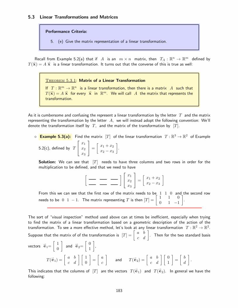
5.3 Linear Transformations and Matrices
Performance Criteria:
5. (e) Give the matrix representation of a linear transformation.
Recall from Example 5.2(a) that if A is an m × n matrix, then TA : Rn → Rm defined by
T (
x) = A
x is a linear transformation. It turns out that the converse of this is true as well:
Theorem 5.3.1: Matrix of a Linear Transformation
If T : Rm → Rn is a linear transformation, then there is a matrix A such that
T (
x) = A
x for every
x in Rm. We will call A the matrix that represents the
transformation.
As it is cumbersome and confusing the represent a linear transformation by the letter T and the matrixrepresenting the transformation by the letter A, we will instead adopt the following convention: We’lldenote the transformation itself by T , and the matrix of the transformation by [T ].
⋄ Example 5.3(a): Find the matrix [T ] of the linear transformation T : R3 → R2 of Example
5.2(c), defined by T
x1x2x3
=
[
x1 + x2x2 − x3
]
.
Solution: We can see that [T ] needs to have three columns and two rows in order for themultiplication to be defined, and that we need to have
[ ]
x1x2x3
=
[
x1 + x2x2 − x3
]
From this we can see that the first row of the matrix needs to be 1 1 0 and the second row
needs to be 0 1 − 1. The matrix representing T is then [T ] =
[
1 1 00 1 −1
]
.
The sort of “visual inspection” method used above can at times be inefficient, especially when tryingto find the matrix of a linear transformation based on a geometric description of the action of thetransformation. To see a more effective method, let’s look at any linear transformation T : R2 → R
2.
Suppose that the matrix of of the transformation is [T ] =
[
a b
c d
]
. Then for the two standard basis
vectors
e1=
[
10
]
and
e2=
[
01
]
,
T (
e1) =
[
a b
c d
] [
10
]
=
[
a
c
]
and T (
e2) =
[
a b
c d
] [
01
]
=
[
b
d
]
.
This indicates that the columns of [T ] are the vectors T (
e1) and T (
e2). In general we have thefollowing:
183

Theorem 5.3.2: Finding the Matrix of a Linear Transformation
Let
e1,
e2, ... ,
em be the standard basis vectors of Rm, and suppose that
T : Rm → Rn is a linear transformation. Then the columns of [T ] are the vectors
obtained when T acts on each of the standard basis vectors
e1,
e2, ... ,
em.We indicate this by
[T ] = [T (
e1) T (
e2) · · · T (em) ]
⋄ Example 5.3(b): Let T be the transformation in R2 that rotates all vectors counterclockwise
by ninety degrees. This is a linear transformation; use the previous theorem to determine its matrix[T ].
Solution: It should be clear that T (
e1) = T
[
10
]
=
[
01
]
and T (
e2) = T
[
01
]
=
[
−10
]
.
Then
[T ] = [T (
e1) T (
e2) ] =
[
0 −11 0
]
The results of this section are particularly powerful from a computational point of view...
Section 5.3 Exercises To Solutions
1. Each of the following transformations T from the Section 5.2 Exercises is linear. Give the matrix[T ] of each.
(a) T
x1x2x3
=
[
2x1 − x3
x1 + x2 + x3
]
(b) T
x1x2x3
=
x1 + x3x2 + x3x1 + x2
(c) T
[
x1x2
]
=
x1 + 2x23x2 − 5x1
x1
(d) T
[
x1
x2
]
=
[
x2
x1 + x2
]
(e) T
[
x1
x2
]
=
[
3x1x1 − x2
]
2. In this exercise we’ll apply Theorem 5.3.2 to find the matrix [T ] of the transformation thatreflects every vector in R
2 across the line y = x.
(a) Sketch the R2 axes, and on that sketch the line y = x and the two standard basis
vectors
e1=
[
10
]
and
e2=
[
01
]
.
(b) Give the vectors T (
e1) and T (
e2).
(c) Give [T ], the matrix of the transformation.
184

3. Now we’ll use Theorem 5.3.2 to find the matrix of the transformation that projects all vectorsonto the line through the origin and the point (4, 3).
(a) Sketch the R2 axes, and then the two standard basis vectors
e1 and
e2, and the vector
v from the origin to the point (4, 3).
(b) Recall that the projection of a vector
u onto a vector
v is given by
projv
u =
u · v
v · v
v .
Noting that projecting on the line through the origin and (4, 3) is the same as projectingon the vector
v from the origin to the point (4, 3), find T (
e1) and T (
e2).
(c) You can now give the matrix [T ] that projects all vectors onto the line through the originand (4, 3). Do so!
4. Repeat the process from Exercise 3 to find the matrix [T ] of the transformation that projectsevery vector on the line through the origin and the point (a, b).
5. In this exercise we’ll determine the matrix of the transformation T that rotates every vector 90degrees counterclockwise (when looking along the positive z-axis toward the origin) around thez-axis, then 90 degrees counterclockwise around the x-axis (again, with counterclockwise beingas one looks along the positive x-axis toward the origin).
(a) Consider the vector
v=
403
. What is the vector
v1 obtained when
v is rotated 90
degrees counterclockwise around the z-axis? What is the vector
v2 obtained when when
v1 is rotated 90 degrees counterclockwise around the x-axis? Note that
v2 = T (
v).
(b) The standard basis vectors in R3 are
e1 =
100
,
e1 =
010
, and
e3 =
001
.
Find T (
e1), T (
e2) and T (
e3).
(c) Give the matrix [T ]. Multiply it times the vector
v from part (a) and see if you get thefinal result of that part,
v2. (You should!)
185

5.4 Compositions of Transformations
Performance Criterion:
5. (f) Find the composition of two transformations.
It is likely that at some point in your past you have seen the concept of the composition of twofunctions; if the functions were denoted by f and g, one composition of them is the new function f g.We call this new function “f of g”, and we must describe how it works. This is simple - for any x,(f g)(x) = f [g(x)]. That is, g acts on x, and f then acts on the result. There is another composition,g f , which is defined the same way (but, of course, in the opposite order). For specific functions, youwere probably asked to find the new rule for these two compositions. Here’s a reminder of how that isdone:
⋄ Example 5.4(a): For the functions f(x) = 2x − 1 and g(x) = 4x − x2, find the formulas forthe composition functions f g and g f .
Solution: Basic algebra gives us
(f g)(x) = f [g(x)] = f [4x− x2] = 2(4x − x2)− 1 = 8x− 2x2 − 1 = −2x2 + 8x− 1
and
(g f)(x) = g[f(x)] = g[2x− 1] = 4(2x− 1)− (2x− 1)2 =
(8x− 4)− (4x2 − 4x+ 1) = 8x− 4− 4x2 + 4x− 1 = −4x2 + 12x − 5
The formulas are then (f g)(x) = −2x2 + 8x− 1 and (g f)(x) = −4x2 + 12x− 5.
Worthy of note here is that the two compositions f g and g f are not the same!One thing that was probably glossed over when you first saw this concept was the fact that the
range (all possible outputs) of the first function to act must fall within the domain (allowable inputs) ofthe second function to act. Suppose, for example, that f(x) =
√x− 4 and g(x) = x2. The function f
will be undefined unless x is at least four; we indicate this by writing f : [4,∞)→ R. This means thatwe need to restrict g in such a way as to make sure that g(x) ≥ 4 if we wish to form the compositionf g. One simple way to do this is to restrict the domain of g to [2,∞). (We could include the interval(−∞,−2] also, but for the sake of simplicity we will just use the positive interval.) The range of g is then[4,∞), which coincides with the domain of f . We now see how these ideas apply to transformations,and we see how to carry out a process like that of Example 5.4(a) for transformations.
⋄ Example 5.4(b): Let S : R3 → R2 and T : R2 → R
2 be defined by
S
x1x2x3
=
[
x21x2x3
]
, T
[
x1x2
]
=
[
x1 + 3x22x2 − x1
]
Determine whether each of the compositions S T and T S exists, and find a formula for eitherof them that do.
186

Solution: Since the domain of S is R3 and the range of T is a subset of R2, the composition
S T does not exist. The range of S falls within the domain of T , so the composition T S doesexist. Its equation is found by
(T S)
x1x2x3
= T
S
x1x2x3
= T
[
x21x2x3
]
=
[
x21 + 3x2x32x2x3 − x21
]
Let’s formally define what we mean by a composition of two transformations.
Definition 5.4.1 Composition of Transformations
Let S : Rp → Rn and T : Rm → R
p be transformations. The composition ofS and T , denoted by S T , is the transformation S T : Rm → R
n defined by
(S T )
x= S(T
x)
for all vectors
x in Rm.
Although the above definition is valid for compositions of any transformations between vector spaces,we are primarily interested in linear transformations. Recall that any linear transformation between vectorspaces can be represented by matrix multiplication for some matrix. Suppose that S : R3 → R
3 andT : R2 → R
3 are linear transformations that can be represented by the matrices
[S] =
3 −1 50 2 14 0 −3
and [T ] =
2 7−6 11 −4
respectively.
⋄ Example 5.4(c): For the transformations S and T just defined, find (S T )
x= (S
T )
[
x1x2
]
. Then find the matrix of the transformation S T .
Solution: We see that
(S T )[
x1x2
]
= S
(
T
[
x1x2
])
= S
2 7−6 11 −4
[
x1x2
]
= S
2x1 + 7x2−6x1 + x2x1 − 4x2
=
3 −1 50 2 14 0 −3
2x1 + 7x2−6x1 + x2x1 − 4x2
187

=
3 −1 50 2 14 0 −3
2x1 + 7x2−6x1 + x2x1 − 4x2
=
3(2x1 + 7x2)− (−6x1 + x2) + 5(x1 − 4x2)0(2x1 + 7x2) + 2(−6x1 + x2) + (x1 − 4x2)4(2x1 + 7x2) + 0(−6x1 + x2)− 3(x1 − 4x2)
=
17x1 + 0x2−11x1 − 2x25x1 + 40x2
From this we can see that the matrix of S T is [S T ] =
17 0−11 −2
5 40
.
Recall that the linear transformations of this example have matrices [S] and [T ], and we find that
[S][T ] =
3 −1 50 2 14 0 −3
2 7−6 11 −4
=
17 0−11 −2
5 40
.
This illustrates the following:
Theorem 5.4.2 Matrix of a Composition
Let S : Rp → Rn and T : Rm → R
p be linear transformations with matrices[S] and [T ]. Then
[S T ] = [S][T ]
Section 5.4 Exercises To Solutions
1. Let R : R2 → R2, S : R2 → R
3 and T : R3 → R2 be defined by
R
[
x1x2
]
=
[
x1x2
x1 − x2
]
, S
[
x1x2
]
=
2x1 + x2
x2
x2 − 3x1
, T
x1x2x3
=
[
x2 − 5
x1 + x3 + 2
]
.
For each of the following compositions, give the declaration statement of the form transformation :Rm → R
n and the formula for the transformation, showing your work as done in Example 5.4(b),and simplify by combining like terms when possible.
(a) S R (b) T S (c) R T (d) S T
2. Let S : R3 → R2 and T : R2 → R
3 be defined by
S
x1x2x3
=
[
2x1 − x3
x1 + x2 + x3
]
and T
[
x1x2
]
=
x1 + 1x2 − 1x1 + x2
.
188

(a) Give both S T and T S in the same sort of way that S and T are given above.Combine like terms in each component, where possible.
(b) Write statements of the the form S T : Rm → Rn for each composition, with the correct
values of m and n.
3. Let S : R2 → R2 and T : R2 → R
3 be defined by
S
x1x2x3
=
x2
x3
x1
and T
[
x1x2
]
=
x1 + 1x2 − 1x1 + x2
.
Only one of S T and T S is possible. Give it in the same sort of way that S and T aregiven above, and write a statement of the form transformation : Rm → R
n, with the correctvalues of m and n.
4. Consider the linear transformations S
[
x
y
]
=
x+ y
2x−3y
, T
[
x
y
]
=
[
5x− y
x+ 4y
]
.
(a) Since both of these are linear transformations, there are matrices [S] and [T ] representingthem. Give those two matrices.
(b) Give equations for either (or both) of the compositions S T and T S that exist.
(c) Give the matrix for either (or both) of the compositions that exist. Label it, with the notation[S T ].
(d) Find either (or both) of [S][T ] and [T ][S] that exist.
(e) What did you notice in parts (c) and (d)? Answer this with a complete sentence.
5. Consider the three transformations
R
x1x2x3
=
[
2x1 − x3
x1 + x2 + x3
]
, S
x1x2x3
=
[
x1x2 + x3
x1
]
, T
x1x2x3
=
x1 + x3x2 + x3x1 + x2
(a) Any time that we have three transformations, there are six potentially possible compositionsof them, with R S being the “first.” list the other five.
(b) Only some of the transformations that you listed are possible. Give each that is, in the sameway that you have been doing, or as is shown in Example 5.4(b) and (c). Be sure to simplifywhere possible.
(c) Two of the transformations are linear, as is one of the compositions of them. Give thematrices of the two that are linear and the matrix of their composition. Verify that Theorem5.4.2 holds.
189

5.5 Transformations and Homogeneous Coordinates
Performance Criteria:
5. (g) Find matrices that perform combinations of dilations, reflections, rota-tions and translations in R
2 using homogenous coordinates.
We are now equipped to return to the applications of rotation and reflection matrices in the context oflinear transformations. We know from Example 5.2(a) that a transformation from R
2 to R2 defined by
multiplication by a matrix is a linear transformation. One should be able to convince oneself geometricallyas well that rotations and reflections are linear.
If we wanted to perform a rotation T followed by a reflection S, this would be done by thecomposition S T , and we know from the previous section that the matrix of S T is simply [S][T ].Using formulas from Chapter 3 to get the matrices [S] and [T ], it is then fairly simple to come upwith a single matrix to perform the desired composition. Transformations like rotations and reflectionsare quite useful in areas like robotics and computer graphics, and when using them we often wish tocompose several such transformations as just described.
In example 5.2(d) we saw that translations like
T
[
x1x2
]
=
[
x1 + a
x2 + b
]
(1)
are not linear, so they do not have matrix representations. What we will find in this section is that ifwe work in the two-dimensional plane z = 1 in R
3, a translation like (1) becomes a shear in R3,
which IS linear. Before looking into how this is done, we first see a method for multiplying a matrixtimes several vectors all at the same time.
⋄ Example 5.5(a): Let A =
[
3 −12 5
]
,
u1 =
[
14
]
,
u2 =
[
7−2
]
,
u3 =
[
33
]
. Find each
of A
u1, A
u2, A
u3.
Solution: A
u1 =
[
−122
]
, A
u2 =
[
234
]
, A
u3 =
[
621
]
.
⋄ Example 5.5(b): Let A be as in the previous example, and let B =
[
1 7 34 −2 3
]
, the
matrix whose columns are
u1,
u2 and
u3 from Example 5.5(a). Compute AB.
Solution: AB =
[
3 −12 5
] [
1 7 34 −2 3
]
=
[
−1 23 622 4 21
]
.
We note in the above two examples that the columns of AB are simply the results of multiplyingeach column of B individually by A. The reason that this is of interest to us is that we will wish toperform a linear transformation, like a rotation, on a geometric object in R
2. Conceptually we wouldthen multiply every point (of which there are infinitely many) of the object by a rotation matrix. Inpractice, if the object is a polygon all we have to do is transform each of the vertices of the polygon
190

and connect the resulting vertices with line segments in order to transform the entire polygon. Let’sdemonstrate with an example. We will utilize the fact that the matrix
A =
[
0 −11 0
]
rotates all points in R2 90 degrees counterclockwise around the origin.
⋄ Example 5.5(c): Find the triangle P ′Q′R′ obtained by ro-tating the triangle PQR shown to the right counterclockwise90 degrees around the origin.
3
5
P Q
R
Solution: We can represent the triangle PQR by the matrix [PQR] =
[
2 4 41 1 2
]
.
From the above discussion we know we can create the new triangle P ′Q′R′ by simply multi-plying the matrix [PQR] representing PQR by the rotation matrix A given above to geta matrix [P ′Q′R′] whose columns are the points P ′, Q′ and R′ of the transformed triangleP ′Q′R′. We then simply plot the vertices P ′, Q′ and R′ and connect them in order to getP ′Q′R′.
[P ′Q′R′] = A [PQR] =
[
0 −11 0
] [
2 4 41 1 2
]
=
[
−1 −1 −22 4 4
]
(2)
On the grid to the right we see the original trianglePQR and the transformed triangle P ′Q′R′ whose ver-tices are given by the columns of the matrix [P ′Q′R′] ob-tained by the multiplication (2) above.
5
5
P Q
RP ′
Q′
R′
In Example 5.5(a) we found that if A =
[
3 −12 5
]
and
u1 =
[
14
]
, then A
u1 =
[
−122
]
.
Note how this result compares with the following example.
⋄ Example 5.5(d): Let C =
3 −1 02 5 00 0 1
,
w =
141
. Find the product C
w.
Solution: C
w=
3 −1 02 5 00 0 1
141
=
−1221
191

Observe carefully how the matrix C was obtained from A by augmenting with a column of zerosand then adding a row of two zeros and a one, and how
w was obtained from
u1 by adding athird component of one. The result of C
w is then the result of A
u1, but also with an additionalcomponent of one. We can thus do R
2 transformations, like rotations and reflections, in the planez = 1 in this manner.
Why would we want to do this? The following example will show that.
⋄ Example 5.5(e): What is the result when the matrix A =
1 0 a
0 1 b
0 0 1
acts on the vector
xh=
x1x21
through multiplication?
Solution: A
xh =
1 0 a
0 1 b
0 0 1
x1x21
=
x1 + a
x2 + b
1
We say that
xh is the homogeneous coordinate vector in R3 for the vector
x =
[
x1x2
]
in
R2, and we can see that the first two components of A
xh are the result of the translation
T
[
x1x2
]
=
[
x1 + a
x2 + b
]
.
A translation is not linear in R2, but it IS linear when performed as a shear in the plane z = 1 in
R3. This allows us to do a translation with a homogenous matrix in R
3.
⋄ Example 5.5(f): Use a homogenous matrix to translate
x =
[
52
]
three units left an one
unit up.
Solution: In this case the homogeneous translation matrix is A =
1 0 −30 1 10 0 1
and the
homogeneous form of
x is
xh =
521
. Multiplying them gives us
A
xh =
1 0 −30 1 10 0 1
521
=
231
,
so the translation of
x is
[
23
]
.
192

4
5
A B
CD
Now we’re finally ready to do something interesting! Consider the squareABCD shown to the right, and suppose that we wish to rotate it 30degrees counterclockwise about its center. We know how to obtaina matrix that rotates objects 30 degrees counterclockwise around theorigin, but not around other points. The idea here is simple, though.Let T be the translation that shifts the square so that its center is atthe origin, and let R30 be a rotation of 30 degrees counterclockwisearound the origin. If we first apply
the transformation T , then R30, then T−1 (to move the square back after rotating it), we willaccomplish what we want. We translate the square to the origin, rotate it there, then move the rotatedsquare back to the original location. This is the composition T−1 R30 T (remember that therightmost transformation acts first!), and from the previous section we know that the matrix of thistransformation is the product [T−1][R30][T ] of the individual transformation matrices. We will needto recall the following from Chapter 3:
Rotation Matrix in R2
For the matrix A =
[
cos θ − sin θ
sin θ cos θ
]
and any position vector
x in R2,
the product A
x is the vector resulting when
x is rotated counterclockwisearound the origin by the angle θ.
⋄ Example 5.5(g): Create a homogenous matrix to rotate the square ABCD 30 degrees coun-terclockwise around its center.
Solution: Note that the transformation T shifts every point three units to the left and twounits down, so T−1 must shift every point three units to the right and two units up. We candetermine the homogeneous matrices of these by using the form demonstrated in Example 5.5(e),and the rotation matrix can be obtained using the formula above, but we need to augment witha column of zeros and add the row 0 0 1. We thus have
[T ] =
1 0 −30 1 −20 0 1
, [T−1] =
1 0 3
0 1 2
0 0 1
, [R30] =
√32 −1
2 0
12
√32 0
0 0 1
.
The matrix that rotates the square 30 degrees counterclockwise around its center is then theproduct [T−1][R30][T ], computed below:
1 0 3
0 1 2
0 0 1
√32 −1
2 0
12
√32 0
0 0 1
1 0 −30 1 −20 0 1
=
√32 −1
28−3
√3
212
√32
1−2√3
2
0 0 1
193

4
5
A B
CD
⋄ Example 5.5(h): Apply the matrix from Example 5.5(g) to thesquare ABCD shown to the right to rotate it 30 degrees counter-clockwise around its center.
Solution: We can represent the square ABCD with a homoge-nous matrix, shown below and to the left. Each column gives thecoordinates of a vertex, with an extry component of one to repre-sent the point in homogeneous coordinates. Converting the entriesof the transformation matrix from Example 5.5(g) to decimal formgives the matrix to the right below.
[ABCD] =
2 4 4 23 3 1 11 1 1 1
, [T−1 R30 T ] =
0.87 −0.50 1.400.50 0.87 −1.230 0 1
To get the coordinates of the vertices of the new square A′B′C ′D′ we let our transformation acton the original through the product [T−1 R30 T ][ABCD] to get the homogeneous matrix ofthe new square, shown below and to the left. The new square is graphed below and to the right,and we can see that it is square ABCD rotated 30 degrees counterclockwise around its center.
[A′B′C ′D′] =
1.64 3.38 4.38 2.642.38 3.38 1.64 0.641 1 1 1
4
5
A′
B′
C′
D′
We end this section with a comment. Pretty much every calculation we have done all term boilsdown to adding and multiplying. If one were to be writing code to do the things you’ve done in thisassignment, you would simply do it as a bunch of multiplications and additions, rather than doing itwith matrices. For example, to rotate the point (x, y) by an angle of θ around the origin we wouldsimply compute the new coordinates (w, z) by
w = x cos θ − y sin θ, z = x sin θ + y cos θ
The advantage of linear algebra for tasks like this is not computational, but conceptual. Without thetheory that we have developed, figuring out how to do transformations like the ones you will see in someof the exercises would be far more difficult!
194

Section 5.5 Exercises To Solutions
For these exercises we will use the following notation, which is not necessarily standard. Those of youwho encounter these ideas in a robotics course will see a standard notation that is somewhat morecomplicated than we need now. Here is what we’ll use.
• Rθ will be a rotation of θ, with the rotation being copunterclockwise if θ is positive, andclockwise if θ is negative.
• T(a,b) will be a translation by a units in the x-direction and b units in the y-direction.
• R(a,b) will be a reflection across the line through the origin and the point (a, b).
Note that we are using R for both rotations and reflections, but which it is in each case should beclear from the subscripts.
1. For each of the following, give the 3 × 3 homogeneous matrix that would be used to performthe given transformation on vectors/points in R
2 expressed in homogeneous coordinates. Youshould not need a formula for the given reflections.
(a) R−90 (b) T(3,−5) (c) R(1,0)
(d) T(1,2) (e) R(1,−1) (f) Rπ/3
2. Use the notation described at the start of these xercises to describe each of the following trans-formations as a composition of rotations, translations and reflections.
(a) A reflection across the line y = 32x followed by a rotation of 50 degrees counterclockwise
around the origin.
(b) A rotation of 50 degrees counterclockwise around the origin followed by a reflection acrossthe line y = 3
2x.
(c) A rotation of 25 degrees clockwise around the point (6,−2).(d) A reflection across the line y = x− 3. (Hint: Translate so that the line goes through the
origin, reflect, translate back.)
3. (a) Find a homogenous matrix that will rotate all points in R2 90 counterclockwise about
the point (2, 3), using homogeneous coordinates.
(b) Consider the triangle PQR shown to the right below. Sketch what you think the resultP ′Q′R′ of the rotation 90 counterclockwise about the point (2, 3) would look like.
(c) Use your answer to (a) and a homogenous coordinaterepresentation of the triangle PQR to find the ro-tated coordinates P ′, Q′ and R′.
(d) Plot the rotated points and draw the rotated triangleP ′Q′R′ on the grid to the right. If it doesn’t looklike what you predicted in (b), figure out which is wrongand correct it.
5
5
P Q
R
195

4. Suppose that we wish to reflect PQR across the line through the origin and at an angle of60 to the positive x-axis, as shown in the picture below and to the right. We already know howto reflect across the x-axis, so we’ll take advantage of that fact. What we want to do is rotatethe line to the x-axis, reflect, then rotate back.
(a) Find the single matrix that does this by multiplying someother matrices. Round the entries of the final matrixto the nearest hundredth, or give them in exact form.
(b) Apply the matrix to the homogenous coordinates of P ,Q and R to get vertices of a new triangle P ′Q′R′.
(c) Draw P ′Q′R′ on the graph to the right. If it doesn’tlook like the reflection of PQR across the line, findyour error and correct it.
5
5
P Q
R
5. Use a method like that of the previous exercise to derive the following formula. You will need touse the facts that the cosine of an angle of a right triangle is the adjacent side over the hypotemuseand the sine of the angle is the opposite side over the hypotenuse.
Reflection Matrix in R2
For the matrix C =
a2 − b2
a2 + b22ab
a2 + b2
2ab
a2 + b2b2 − a2
a2 + b2
and any position vector
x in
R2, the product C
x is the vector resulting when
x is reflected across the linecontaining the origin and the point (a, b).
6. Find a single homogeneous matrix that will reflectPQR across the line through the point (0, 1) and atan angle of 60 to the x-axis, shown on the graph to theright. Test your result as you have been. Round the en-tries of the matrix to the nearest hundredth, or givethem in exact form.
5
5
P Q
R
196

5.6 An Introduction to Eigenvalues and Eigenvectors
Performance Criteria:
5. (h) Determine whether a given vector is an eigenvector for a matrix; if it is,give the corresponding eigenvalue.
(i) Determine eigenvectors and corresponding eigenvalues for linear trans-formations in R
2 or R3 that are described geometrically.
Recall that the two main features of a vector in Rn are direction and magnitude. In general, when
we multiply a vector
x in Rn by an n×n matrix A, the result A
x is a new vector in Rn whose
direction and magnitude are different than those of
x. For every square matrix A there are somevectors whose directions are not changed (other than perhaps having their directions reversed) whenmultiplied by the matrix. That is, multiplying
x by A gives the same result as multiplying
x bya scalar. It is very useful for certain applications to identify which vectors those are, and what thecorresponding scalar is. Let’s use the following example to get started:
⋄ Example 5.6(a): Multiply A =
[
−4 −63 5
]
times
u =
[
13
]
and
v =
[
2−1
]
and
determine whether multiplication by A is the same as multiplying by a scalar in either case.
Solution:
A
u =
[
−4 −63 5
] [
13
]
=
[
−2218
]
, A
v =
[
−4 −63 5
] [
2−1
]
=
[
−21
]
For the first multiplication there appears to be nothing special going on. For the second multipli-cation, the effect of multiplying
v by A is the same as simply multiplying
v by −1. Notealso that
[
−4 −63 5
] [
−63
]
=
[
6−3
]
,
[
−4 −63 5
] [
8−4
]
=
[
−84
]
It appears that if we multiply any scalar multiple of
v by A the same thing happens; the resultis simply the negative of the vector. That is, A
x = (−1)
x for every scalar multiple of
x.
We say that
v =
[
2−1
]
and all of its scalar multiples are eigenvectors of A, with
corresponding eigenvalue −1. Here is the formal definition of an eigenvalue and eigenvector:
Definition 5.6.1: Eigenvalues and Eigenvectors
A scalar λ is called an eigenvalue of a matrix A if there is a nonzero vector
x such thatA
x= λ
x .
The vector
x is an eigenvector corresponding to the eigenvalue λ.
197

Make special note of this:
An eigenvector must be a nonzero vector, but zero IS allowed as an eigenvalue.
One comment is in order at this point. Suppose that
x has n components. Then λ
x does as well,so A must have n rows. However, for the multiplication A
x to be possible, A must also haven columns. For this reason, only square matrices have eigenvalues and eigenvectors. We now see howto determine whether a vector is an eigenvector of a matrix.
⋄ Example 5.6(b): Determine whether either of
w1 =
[
4−1
]
and
w2 =
[
−33
]
are eigen-
vectors for the matrix A =
[
−4 −63 5
]
of Example 5.6(a). If either is, give the corresponding
eigenvalue.
Solution: We see that
A
w1 =
[
−4 −63 5
] [
4−1
]
=
[
−107
]
and A
w2 =
[
−4 −63 5
] [
−33
]
=
[
−66
]
w1 is not an eigenvector of A because there is no scalar λ such that A
w1 is equal to λ
w1.
w2 IS an eigenvector, with corresponding eigenvalue λ = 2, because A
w2 = 2
w2.
Note that for the 2× 2 matrix A of Examples 5.6(a) and (b) we have seen two eigenvalues now.It turns out that those are the only two eigenvalues, which illustrates the following:
Theorem 5.6.2: The number of eigenvalues of an n× n matrix is at most n.
Do not let the use of the Greek letter lambda intimidate you - it is simply some scalar! It is traditionto use λ to represent eigenvalues. Now suppose that
x is an eigenvector of an n × n matrix A,with corresponding eigenvalue λ, and let c be any scalar. Then for the vector c
x we have
A(c
x) = c(A
x) = c(λ
x) = (cλ)
x = λ(c
x)
This shows that any scalar multiple of
x is also an eigenvector of A with the same eigenvalue λ.We saw this in Example 5.6(a). The set of all scalar multiples of
x is of course a subspace of Rn,
and we call it the eigenspace corresponding to λ.
x, or any scalar multiple of it, is a basis for theeigenspace. The two eigenspaces you have seen so far have dimension one, but an eigenspace can havea higher dimension.
Definition 5.6.3: Eigenspace Corresponding to an Eigenvalue
For a given eigenvalue λj of an n×n matrix A, the eigenspace Ej correspondingto λ is the set of all eigenvectors corresponding to λj . It is a subspace of R
n.
198

So far we have been looking at eigenvectors and eigenvalues from a purely algebraic viewpoint, bylooking to see if the equation A
x= λ
x held for some vector
x and some scalar λ. It is useful to havesome geometric understanding of eigenvectors and eigenvalues as well. In the next two examples weconsider eigenvectors and eigenvalues of two linear transformations in R
2 from a geometric standpoint.Although we have defined eigenvalues in terms of matrices, recall that any linear transformation T canbe represented by a matrix T , so it makes sense to talk about eigenvectors and eigenvalues of atransformation, as long as it is linear. We simply substitute the equation T(
x) = λ
x, which tells usthat
x is an eigenvector if the action of T on it leaves its direction unchanged or opposite of whatit was (or, in the case of λ = 0, “shrinks it to the zero vector”).
⋄ Example 5.6(c): The transformation T that reflects very vector in R2 over the line l with
equation y = 12x is a linear transformation. Determine the eigenvectors and corresponding
eigenvalues for this transformation.
x= T (
x)
u
T (
u)
v
T (
v)
l
x
y
Solution: We begin by observing that any vector that lies on l willbe unchanged by the reflection, so it will be an eigenvector, witheigenvalue λ = 1. These vectors are all the scalar multiples of
x =
[
21
]
; see the picture to the right. A vector not on the
line,
u, is shown along with its reflection T (
u) as well. Wecan see that its direction is changed, so it is not an eigenvector.However, for any vector
v that is perpendicular to l we haveT (
v) = −
v. Therefore any such vector is an eigenvector witheigenvalue λ = −1. Those vectors are all the scalar multiples of
x =
[
−12
]
.
⋄ Example 5.6(d): Let T be the transformation T that rotates every vector in R2 by
thirty degrees counterclockwise; this is a linear transformation. Determine the eigenvectors andcorresponding eigenvalues for this transformation.
Solution: Because every vector in R2 will be rotated by thirty degrees, the direction of every
vector will be altered, so there are no eigenvectors for this transformation.
Our conclusion in Example 5.6(d) is correct in one sense, but incorrect in another. Geometrically, ina way that we can see, the conclusion is correct. Algebraically, the transformation has eigenvectors,but their components are complex numbers, and the corresponding eigenvalues are complex numbers aswell. In this course we will consider only real eigenvectors and eigenvalues.
Section 5.6 Exercises To Solutions
1. Consider the matrix A =
[
1 1
−2 4
]
.
(a) Find A
x for each of the following vectors:
x1 =
[
36
]
,
x2 =
[
2−1
]
,
x3 =
[
15
]
,
x4 =
[
−3−3
]
,
x5 =
[
22
]
199

(b) Give the vectors from part (a) that are eigenvectors and, for each, give the correspondingeigenvalue.
(c) Give one of the eigenvalues that you have found. Then give the general form for anyeigenvector corresponding to that eigenvalue.
(d) Repeat part (c) for the other eigenvalue that you have found.
2. For each of the following a matrix is given, along with several vectors. Determine which of thevectors are eigenvectors, and give the corresponding eigenvalue for each.
(a) A =
[
2 7−1 −6
]
,
u1 =
[
12
]
,
u2 =
[
−11
]
,
u3 =
[
−71
]
,
u4 =
[
11
]
(b) A =
[
1 22 4
]
,
v1 =
[
12
]
,
v2 =
[
−11
]
,
v3 =
[
11
]
,
v4 =
[
2−1
]
(c) A =
1 1 00 2 00 −1 4
,
w1 =
100
,
w2 =
001
,
w3 =
111
,
w4 =
221
(d) A =
1 −1 0−1 2 −10 −1 1
,
u1=
10−1
,
u2=
001
,
u3=
111
,
u4 =
1−21
,
u5 =
221
3. Suppose that a matrix A has eigenvectors
x1 =
31−1
and
x2 =
102
with
respective eigenvalues λ1 = 2 and λ2 = −1. Which of the following are also eigenvectors, andwhat are their corresponding eigenvalues?
v1 =
−60
−12
,
v2 =
201
,
v3 =
62−2
,
v4 =
−32
−1212
,
v5 =
204
4. The previous exercise is based on the idea that if
x is an eigenvector of A, then any scalarmultiple of
x is also an eigenvector, with the same eigenvalue. This exercise will show that therecan be linearly independent eigenvectors that share the same eigenvalue. Determine which of thevectors below are eigenvectors for the matrix
A =
3 2 42 0 24 2 3
.
For those that are, give the corresponding eigenvalue.
u1 =
10−2
,
u2 =
1−20
,
u3 =
12−1
,
u4 =
0−21
,
u5 =
212
200

5. For each transformation described geometrically, give as many independent eigenvectors, and theircorresponding eigenvalues, as you can. Keep in mind that any vectors that become the zero vectorunder the transformation, with zero as an eigenvalue.
(a) The transformation that reflects every vector in R2 across the y-axis.
(b) The transformation that projects every vector in R2 onto the y-axis.
(c) The transformation that projects every vector in R2 onto the line y = 3x.
(d) The transformation that reflects every vector in R3 across the yz-plane.
(e) The transformation that rotates every vector in R3 90 degrees around the z-axis.
(f) The transformation that projects every vector in R3 onto the xz-plane.
(g) The transformation that reflects every vector in R3 across the plane with equation z = −y.
(Hint: Sketch a picture of the graph of this equation in the yz-plane.)
201

5.7 Finding Eigenvalues and Eigenvectors
Performance Criteria:
5. (j) Find the characteristic polynomial for a 2× 2 or 3× 3 matrix. Use itto find the eigenvalues of the matrix.
(k) Give the eigenspace Ej corresponding to an eigenvalue λj of a matrix.
(l) Determine the principal stresses and the orientation of the principal axesfor a two-dimensional stress element.
So where are we now? We know what eigenvectors, eigenvalues and eigenspaces are, and we knowhow to determine whether a vector is an eigenvector of a matrix. There are two big questions at thispoint:
• Why do we care about eigenvalues and eigenvectors?
• If we are just given a square matrix A, how do we find its eigenvalues and eigenvectors?
We will not see the answer to the first question until the end of this section. First we’ll address thesecond question.
Finding Eigenvalues
We begin by rearranging the eigenvalue/eigenvector equation A
x = λ
x a little. First, we cansubtract λ
x from both sides to getA
x −λ
x =
0 .
Note that the right side of this equation must be the zero vector, because both A
x and λ
x arevectors. At this point we want to factor
x out of the left side, but if we do so carelessly we will get afactor of A−λ, which makes no sense because A is a matrix and λ is a scalar! Note, however, thatwe can replace
x with I
x, thus we can replace λ
x with (λI)
x, allowing us to factor
x out:
A
x −λ
x =
0
A
x − (λI)
x =
0
(A− λI)
x =
0
Now A− λI is just a matrix - let’s call it B for now. Any nonzero (by definition) vector
x that is a
solution to B
x =
0 is an eigenvector for A. Clearly the zero vector is a solution to B
x =
0, andif B is invertible that will be the only solution. But since eigenvectors are nonzero vectors, A willhave eigenvectors only if B is not invertible. Recall that one test for invertibility of a matrix is whetherits determinant is nonzero. For B to not be invertible, then, its determinant must be zero. But B isA − λI, so we want to find values of λ for which det(A − λI) = 0. (Note that the determinantof a matrix is a scalar, so the zero here is just the scalar zero.) We introduce a bit of special languagethat we use to discuss what is happening here:
Definition 5.7.1: Characteristic Polynomial and Equation
Taking λ to be an unknown, det(A−λI) is a polynomial called the characteristicpolynomial of A. The equation det(A − λI) = 0 is called the characteristicequation for A, and its solutions are the eigenvalues of A.
202

Before looking at a specific example, you would probably find it useful to go back and look atExamples 3.8(a), (b) and (c), and to recall the following.
Determinant of a 2× 2 Matrix
The determinant of the matrix
[
a b
c d
]
is det(A) = ad− bc.
Determinant of a 3× 3 Matrix
To find the determinant of a 3× 3 matrix,
• Augment the matrix with its first two columns.
• Find the product down each of the three complete “downward diagonals”of the augmented matrix, and the product up each of the three “upwarddiagonals.”
• Add the products from the downward diagonals and subtract each of theproducts from the upward diagonals. The result is the determinant.
Now we’re ready to look at a specific example of how to find the eigenvalues of a matrix.
⋄ Example 5.7(a): Find the eigenvalues of the matrix A =
[
−4 −63 5
]
.
Solution: We need to find the characteristic polynomial det(A− λI), then set it equal to zeroand solve.
A− λI =
[
−4 −63 5
]
− λ
[
1 00 1
]
=
[
−4 −63 5
]
−[
λ 00 λ
]
=
[
−4− λ −63 5− λ
]
det(A− λI) = (−4− λ)(5− λ)− (3)(−6)) = (−20− λ+ λ2) + 18 = λ2 − λ− 2
We now factor this and set it equal to zero to find the eigenvalues:
λ2 − λ− 2 = (λ− 2)(λ+ 1) = 0 =⇒ λ = 2,−1
We use subscripts to distinguish the different eigenvalues: λ1 = 2, λ2 = −1.
Finding Eigenvectors
We now need to find the eigenvectors or, more generally, the eigenspaces, corresponding to eacheigenvalue. We defined eigenspaces in the previous section, but here we will give a slightly different (butequivalent) definition.
203

Definition 5.7.2: Eigenspace Corresponding to an Eigenvalue
For a given eigenvalue λj of an n×n matrix A, the eigenspace Ej correspondingto λj is the set of all solutions to the equation
(A− λjI)
x =
0 .
It is a subspace of Rn.
Note that we indicate the correspondence of an eigenspace with an eigenvalue by subscripting themwith the same number.
⋄ Example 5.7(b): Find the eigenspace E1 of the matrix A =
[
−4 −63 5
]
corresponding to
the eigenvalue λ1 = 2.
Solution: For λ1 = 2 we have A− λI =
[
−4 −63 5
]
−[
2 00 2
]
=
[
−6 −63 3
]
The augmented matrix of the system (A−λI)
x =
0 is then
[
−6 −6 03 3 0
]
, which reduces
to
[
1 1 00 0 0
]
. The top row represents the equation x1 + x2 = 0 so any values of x1 and
x2 that make this true will give us an eigenvector so, for example, we can take
x to be
[
−11
]
.
The eigenspace corresponding to λ1 = 2 can then be described by either of
E1 =
t
[
−11
]
or E1 = span
([
−11
])
It would be beneficial for the reader to repeat the above process for the second eigenvalue λ2 = −1 andverify that
E2 =
t
[
−21
]
.
When first seen, the whole process for finding eigenvalues and eigenvectors can be a bit bewildering!Here is a summary of the process:
Finding Eigenvalues and Bases for Eigenspaces
The following procedure will give the eigenvalues and corresponding eigenspaces fora square matrix A.
1) Find det(A− λI). This is the characteristic polynomial of A.
2) Set the characteristic polynomial equal to zero and solve for λ to get theeigenvalues.
3) For a given eigenvalue λi, solve the system (A− λjI)
x =
0. The set ofsolutions is the eigenspace corresponding to λj. The vector or vectors whoselinear combinations make up the eigenspace are a basis for the eigenspace.
204

⋄ Example 5.7(c): Give the characteristic polynomial of the matrix
A =
1 −1 0−1 2 −10 −1 1
and use it to determine the eigenvalues. Then, given that one of the eigenvalues is λ1 = 3, givethe corresponding eigenspace E1.
Solution: First we see that
A− λI =
1 −1 0−1 2 −10 −1 1
− λ
1 0 00 1 00 0 1
=
1 −1 0−1 2 −10 −1 1
−
λ 0 00 λ 00 0 λ
=
1− λ −1 0−1 2− λ −10 −1 1− λ
The characteristic polynomial is
det(A− λI) = det
1− λ −1 0−1 2− λ −10 −1 1− λ
= (1− λ)(2 − λ)(1− λ)− (1− λ)− (1− λ)
= (1− λ)(2 − λ)(1− λ)− 2(1 − λ).
Ordinarily we would just multiply everything out, combine like terms and solve by factoring usingalgebra methods or a computational tool. In this case, however, we can factor (1 − λ) out ofboth terms to get
det(A− λI) = (1− λ)[(2 − λ)(1− λ)− 2]
= (1− λ)[(2 − 3λ+ λ2)− 2]
= (1− λ)(λ2 − 3λ)
= λ(1− λ)(λ− 3).
This last expression is the characteristic polynomial, in factored form, and we can see that theeigenvalues are 0, 1 and 3.
To find the eigenspace corresponding to λ1 = 3 we solve the characteristic equation(A− λI)
x =
0 for λ = 3. First we compute
A− λI =
1 −1 0−1 2 −10 −1 1
− 3
1 0 00 1 00 0 1
=
−2 −1 0−1 −1 −10 −1 −2
205

The augmented matrix for (A− λI)
x =
0 is shown below and to the left, and its row reducedform is below and to the right.
−2 −1 0 0−1 −1 −1 00 −1 −2 0
rref=⇒
1 0 −1 00 1 2 00 0 0 0
(1)
We see that x3 is a free variable. Letting x3 = t and solving x2+2x3 = 0 gives us x2 = −2t.Solving x1 − x3 = 0 gives us x1 = t. The solution to (A − λI)
x =
0 is then the set ofvectors of the form
t
−2tt
= t
1−21
and the eigenspace corresponding to λ1 = 3 is
E1 =
t
1−21
.
We can vary the above process slightly as follows. After obtaining the row-reduced form (1) we getthe equation x2 + 2x3 = 0, and we can see that x2 = −2 and x3 = 1 is a solution. For thatchoice of x3 the first equation x1 − x3 = 0 gives us that x1 = 1 as well. This gives us the single
eigenvector
1−21
, and the corresponding eigenspace is all scalar multiples of that vector, as shown
above.
An Application - Principal Stress
Figure 5.7(a) below and to the left shows a cantilevered beam embedded in a wall at its right end.There is a force acting downward on the left end of the beam, due to the weight of the beam andperhaps a load applied to the end of the beam. The small square stress element shown on the side ofthe beam toward us is an imaginary square extending back through to the far side of the beam. Thatelement is subject to stresses of tension (indicated by the little arrows) and compression, as well assome shear stress. The element is blown up in Figure 5.7(b) and all of the stresses on it are shown.σx and σy are normal stresses, and τxy and τyx are shear stresses. The fact that the elementis not rotating gives us that τxy = τyx.
Force
Figure 5.7(a)
y
xσxσx
σy
σy
τxy
τxy
τyx
τyx
τxy = τyx
Figure 5.7(b)
yp
xp
σx
σx
σy
σy
θ
Figure 5.7(c)
We can rotate the stress element about its center and the stresses will all change as we do that.
206

There is one angle of rotation we are particularly interested in. If we rotate by a particular angle θ allof the stress will be normal, with no shear stresses. This is depicted in Figure 5.7(c) above and to theright. The new axes xp and yp are called the principal axes. The two normal stresses for thisorientation of the stress element are called principal stresses, and one of them is the greatest stressat the location of the stress element in the beam. The key to finding the principal stresses and theirdirections is eigenvalues and eigenvectors! We begin by setting up a stress matrix:
[
σx τxyτyx σy
]
,
keeping in mind that τxy = τyx. Stresses oriented in the directions of the arrows in Figure 5.7(b) aretaken to be positive, any oriented opposite of those arrows are considered to be negative. We then findthe eigenvalues and corresponding eigenvectors of the stress matrix. The eigenvalues give us the normalstresses in the directions of their corresponding eigenvectors. If we reorient the stress element to havethe principal stresses as its normal stresses there will be no shear stresses. Let’s see how this happensin practice.
⋄ Example 5.7(d): The normal and shear stresses ona stress element are shown to the right. Determine theprincipal stresses and the angle of rotation (from thepositive x-axis, as shown in Figure 5.7(c)). Sketch thestress element and indicate the stresses when the normalstresses are the principal stresses. Give values in decimalform, rounded to the nearest tenth.
y
x70MPa
70MPa
50 MPa
50 MPa
20MPa
Solution: Accounting for the orientations of the stresses, the stress matrix is
[
−70 −20−20 50
]
.
The characteristic polynomial is (−70 − λ)(50 − λ) − (−20)2 = λ2 + 20λ − 3900. Setting itequal to zero and solving with the quadratic formula gives us λ = −73.2, 53.2. The augmentedmatrices for the system (A− λI)
x =
0 for each of these eigenvalues are[
3.2 −20 0−20 126.2 0
]
and
[
−126.2 −20 0−20 −3.2 0
]
.
These will not row-reduce to give a second row of zeros because of needing to round the eigen-values, so we assume that they reduce to
[
3.2 −20 00 0 0
]
and
[
−126.2 −20 00 0 0
]
.
An eigenvector for λ1 = −73.2 is
[
203.2
]
and for λ = 53.2 we get the eigenvector
[
−20126.2
]
.
We can verify that these vectors are essentially perpendic-ular by taking their dot product and seeing that it is veryclose to zero, and would be if we hadn’t rounded our eigen-values. The angle of the first vector with the x-axis is
θ = tan−1 3.2
20= 9.1. (Draw a sketch of the vector to
see how we get this.) The stress element reoriented alongthe principal axes, along with the principal stresses, is shownto the right.
yp
xp
73.2 MPa
73.2 MPa
53.2MPa
53.2MPa
9.1
207

When analyzing beams we generally encounter stress elements like the one in Example 5.7(d), withtension in one direction (the y- and yp-directions in this case) and compression in the other (here in thex- and xp-directions). When analyzing a sheet structure we can see tension in both normal directions,and something like soil underground can exhibit compression in both normal directions. Those caseswill arise in the exercises.
Section 5.7 Exercises To Solutions
1. Use the method of Example 5.7(b) to find the eigenspace of A =
[
−4 −63 5
]
corresponding
to λ2 = −1.
2. Find the eigenvalues and corresponding eigenspaces for each of the following matrices. Answersare given in the back of the book, but check your answers yourself by multiplying the matrix timeseach basis eigenvector to make sure the result is the same as multiplying the eigenvector by theeigenvalue.
(a)
[
8 32 7
]
(b)
[
2 −1−1 2
]
(c)
[
2 −4−1 −1
]
3. For each of the following a matrix is given, and it’s action as a transformation on vectors/pointsin R
2 is described. Find the eigenvectors and eigenspaces, and make sure that your results makesense for the transformation described.
(a)
[
0 11 0
]
, which reflects vectors across the line y = x.
(b)
[
12 −1
2
−12
12
]
, which projects vectors onto the line y = −x.
(c)
[
−1 00 1
]
, which reflects vectors across the y-axis.
4. Follow a process like the last half of Example 5.7(c) to find the eigenspaces E2 and E3 of
A =
1 −1 0−1 2 −10 −1 1
corresponding to the eigenvalues λ2 = 1 and λ3 = 0.
5. Consider the matrix A =
4 0 1−2 1 0−2 0 1
.
(a) Find characteristic polynomial by computing det(A− λI). As in Example 5.7(c), you willinitially have two terms that both have a factor of 1−λ in them. Do not expand (multiplyout) these terms - instead, factor the common factor of 1 − λ out of both, then combineand simplify the rest, as done in that example.
208

(b) Give the characteristic equation for matrix A, which is obtained by setting the characteristicpolynomial equal to zero. Remember that you are doing this because the equation A
x =λ
x will only have solutions
x 6=
0 if det(A− λI) = 0. Find the solutions (eigenvalues)of the equation by factoring the part that is not already factored.
(c) One of your eigenvalues should be one; let’s refer to it as λ1. Find a basis for the eigenspace
E1 corresponding to λ = 1 by solving the equation (A− I)
x =
0. ((A− λI) becomes(A− I) because λ1 = 1.) Conclude by giving the eigenspace E1 using correct notation.
(d) Give the eigenspaces corresponding to the other two eigenvalues. Make it clear whicheigenspace is associated with which eigenvalue.
(e) Check your answers by multiplying each eigenvector by the original matrix A to see if theresult is the same as multiplying the eigenvector by the corresponding eigenvalue. In otherwords, if the eigenvector is
x, check to see that A
x = λ
x.
6. (a) For A =
1 2 16 −1 0−1 −2 −1
, find characteristic polynomial. In this case you can’t
factor something out as in Example 5.7(c), so you must multiply everything out.
(b) Give the characteristic equation for matrix A, which is obtained by setting the characteristicpolynomial equal to zero. You should be able to solve it by first factoring −λ out, thenfactoring the remaining quadratic. Do this and give the eigenvalues.
(c) Give the eigenspaces corresponding to the eigenvalues. Make it clear which eigenspace isassociated with which eigenvalue.
7. (a) Find characteristic polynomial for A =
−2 −4 2−2 1 24 2 5
. You again can’t factor
something out, so just have multiply out (carefully!) and combine like terms.
(b) Use Wolfram Alpha or some other tool to factor the characteristic polynomial. (Just usex instead of λ when doing this.) Set the result equal to zero (giving the characteristicequation) and solve to get the eigenvalues.
(c) Give the eigenspaces corresponding to the eigenvalues, again making it clear which eigenspaceis associated with which eigenvalue.
8. (a) Computing det(A− λI) for A =
0 0 2−3 1 60 0 −1
will directly result in a factored
form of the characteristic polynomial of A. Give it.
(b) Give the eigenvalues.
(c) Find the eigenspaces corresponding to the eigenvalues by solving (A− λI)
x =
0 for eacheigenvalue. For one eigenvalue you will have two free variables, resulting in an eigenspace ofdimension two (with two independent basis eigenvectors).
209

9. Find the eigenvalues and eigenspaces for A =
7 0 −3−9 −2 318 0 −8
, using a tool if necessary
for factoring the characteristic polynomial. As with Exercise 7, there are only two eigenspaces,and one of them has dimension two.
10. So far, every n × n matrix we have worked with has had n linearly independent eigenvectors,perhaps with fewer eigenvalues (Exercises 7 and 8). The matrix
A =
1 1 00 2 00 −1 2
has only two eigenvalues and only two independent eigenvectors. Find the eigenvalues and eigen-vectors.
11. For each of the following a stress element is given, along with its normal and shear stresses.Determine the principal stresses and their eigenvectors. Then determine the angle between theprincipal xp-axis and the original x-axis, and whether the angle is positive or negative, followingthe standard convention that counterclockwise is positive and clockwise is negative. Sketchthe rotated stress element, showing the angle of rotation of the axes and the principal stresses,indicating whether each is tension or compression by the direction of its arrow, as done in Example5.7(d).
(a)
y
x30MPa
30MPa
50 MPa
50 MPa
10MPa
(b)
y
x60MPa
60MPa
25 MPa
25 MPa
45MPa
(c)
y
x80MPa
80MPa
50 MPa
50 MPa
20MPa
(d)
y
x40MPa
40MPa
100 MPa
100 MPa
35MPa
210

5.8 Diagonalization of Matrices
Performance Criterion:
5. (m) Diagonalize a matrix; know the forms of the matrices P and D fromP−1AP = D.
We begin with an example involving the matrix A from Examples 5.5(a) and (b).
⋄ Example 5.8(a): For A =
[
−4 −63 5
]
and P =
[
−1 −21 1
]
, find the product P−1AP .
Solution: First we obtain P−1 =1
(−1)(1) − (1)(−2)
[
1 2−1 −1
]
=
[
1 2−1 −1
]
. Then
P−1AP =
[
1 2−1 −1
] [
−4 −63 5
] [
−1 −21 1
]
=
[
2 00 −1
]
We want to make note of a few things here:
• The columns of the matrix P are eigenvectors for A.
• The matrix D = P−1AP is a diagonal matrix.
• The diagonal entries of D are the eigenvalues of A, in the order of the corresponding eigenvectorsin P .
For a square matrix A, the process of creating such a matrix D in this manner is called diagonalizationof A. This cannot always be done, but often it can. (We will fret about exactly when it can be donelater.) The point of the rest of this section is to see a use or two of this idea.
Before getting to the key application of this section we will consider the following. Suppose thatwe wish to find the kth power of a 2 × 2 matrix A with eigenvalues λ1 and λ2 and havingcorresponding eigenvectors that are the columns of P . Then solving P−1AP = D for A givesA = PDP−1 and
Ak = (PDP−1)k = (PDP−1)(PDP−1) · · · (PDP−1)
= PD(P−1P )D(P−1P ) · · · (P−1P )DP−1
= PDDD · · ·DP−1
= PDkP−1
= P
[
λ1 00 λ2
]k
P−1
= P
[
λk1 00 λk
2
]
P−1
Therefore, once we have determined the eigenvalues and eigenvectors of A we can simply take eacheigenvector to the kth power, then put the results in a diagonal matrix and multiply once by P on theleft and P−1 on the right.
211

⋄ Example 5.8(b): Diagonalize the matrix A =
3 12 −21−1 −6 130 −2 6
.
Solution: First we find the eigenvalues by solving det(A− λI) = 0:
det
3− λ 12 −21−1 −6− λ 130 −2 6− λ
= (3− λ)(−6− λ)(6 − λ)− 42 + 26(3 − λ) + 12(6− λ)
= (−18 + 3λ+ λ2)(6− λ)− 42 + 78 − 26λ + 72 − 12λ
= −108 + 18λ+ 18λ− 3λ2 + 6λ2 − λ3 + 108 − 38λ
= −λ3 + 3λ2 − 2λ
= −λ(λ2 − 3λ+ 2)
= −λ(λ− 2)(λ− 1)
The eigenvalues of A are then λ = 0, 1, 2. We now find an eigenvector corresponding toλ = 0 by solving the system (A− λI)
x= 0. The augmented matrix and its row-reduced formare shown below:
3 12 −21 0−1 −6 13 00 −2 6 0
=⇒
1 0 5 00 1 −3 00 0 0 0
=⇒Let x3 = 1.Then x2 = 3and x1 = −5
The eigenspace corresponding to the eigenvalue λ = 0 is then the span of the vector
v1=[−5, 3, 1]. For λ = 1 we have
2 12 −21 0−1 −7 13 00 −2 5 0
=⇒
1 0 92 0
0 1 −52 0
0 0 0 0
=⇒Let x3 = 2.Then x2 = 5and x1 = −9
The eigenspace corresponding to the eigenvalue λ = 1 is then the span of the vector
v2=[−9, 5, 2] (obtained by multiplying the solution vector by two in order to get a vector with integercomponents). Finally, for λ = 2 we have
1 12 −21 0−1 −8 13 00 −2 4 0
=⇒
1 0 3 00 1 −2 00 0 0 0
=⇒Let x3 = 1.Then x2 = 2and x1 = −3
so the eigenspace corresponding to the eigenvalue λ = 2 is then the span of the vector
v3=[−3, 2, 1]. The diagonalization of A is then D = P−1AP , where
D =
0 0 00 1 00 0 2
and P =
−5 −9 −33 5 21 2 1
212
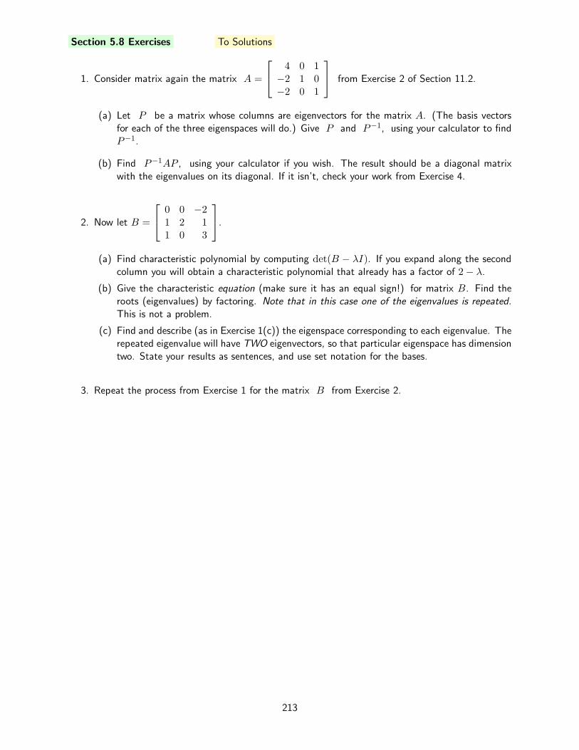
Section 5.8 Exercises To Solutions
1. Consider matrix again the matrix A =
4 0 1−2 1 0−2 0 1
from Exercise 2 of Section 11.2.
(a) Let P be a matrix whose columns are eigenvectors for the matrix A. (The basis vectorsfor each of the three eigenspaces will do.) Give P and P−1, using your calculator to findP−1.
(b) Find P−1AP , using your calculator if you wish. The result should be a diagonal matrixwith the eigenvalues on its diagonal. If it isn’t, check your work from Exercise 4.
2. Now let B =
0 0 −21 2 11 0 3
.
(a) Find characteristic polynomial by computing det(B − λI). If you expand along the secondcolumn you will obtain a characteristic polynomial that already has a factor of 2− λ.
(b) Give the characteristic equation (make sure it has an equal sign!) for matrix B. Find theroots (eigenvalues) by factoring. Note that in this case one of the eigenvalues is repeated.This is not a problem.
(c) Find and describe (as in Exercise 1(c)) the eigenspace corresponding to each eigenvalue. Therepeated eigenvalue will have TWO eigenvectors, so that particular eigenspace has dimensiontwo. State your results as sentences, and use set notation for the bases.
3. Repeat the process from Exercise 1 for the matrix B from Exercise 2.
213

5.9 Solving Systems of Differential Equations
Performance Criteria:
5. (n) Write a system of linear differential equations in matrix-vector form.Write the initial conditions in vector form.
(0) Solve a system of two linear differential equations; solve an initial valueproblem for a system of two linear differential equations.
We now get to the centerpiece of this section. Recall that the solution to the initial value problemx′(t) = kx(t), x(0) = C is x(t) = Cekt. Now let’s consider the system of two differentialequations
x′1 = x1 + 2x2
x′2 = 3x1 + 2x2,
where x1 and x2 are functions of t. Note that the two equations are coupled; the equationcontaining the derivative x′1 contains the function x1 itself, but also contains x2. The same sortof situation occurs with x′2. The key to solving this system is to uncouple the two equations, andeigenvalues and eigenvectors will allow us to do that!
We will also add in the initial conditions x1(0) = 10, x2(0) = 5. If we let
x=
[
x1x2
]
we can
rewrite the system of equations and initial conditions as follows:
[
x′1x′2
]
=
[
1 2
3 2
] [
x1x2
]
,
[
x1(0)x2(0)
]
=
[
105
]
which can be condensed to
x′= A
x,
x (0) =
[
105
]
(1)
This is the matrix initial value problem that is completely analogous to x′(t) = kx(t), x(0) = C.
Before proceeding farther we note that the matrix A has eigenvectors
[
23
]
and
[
−11
]
with
corresponding eigenvalues λ = 4 and λ = −1. Thus, if P =
[
2 −13 1
]
we then have P−1AP =
D =
[
4 0
0 −1
]
and A = PDP−1.
We can substitute this last expression for A into the vector differential equation in (1) to get
x′= PDP−1
x. If we now multiply both sides on the left by P−1 we get P−1
x′= DP−1
x. We now
let
y= P−1
x; Since P−1 is simply a matrix of constants, we then have
y′= (P−1
x)′ = P−1
x′also.
Making these two substitutions into P−1
x′= DP−1
x gives us
y′= D
y. By the same substitutionwe also have
y (0) = P−1
x (0). We now have the new initial value problem
y′= D
y,
y (0) = P−1
x (0). (3)
Here the vector
y is simply the unknown vector
y=
[
y1y2
]
and
y (0) =
[
y1(0)y2(0)
]
which can be
determined by
y (0) = P−1
x (0). Because the coefficient matrix of the system in (3) is diagonal,
214

the two differential equations can be uncoupled and solved to find
y. Now since
y= P−1
x we alsohave
x= P
y, so after we find
y we can find
x by simply multiplying
y by P .
So now it is time for you to make all of this happen!
Section 5.9 Exercises To Solutions
1. Write the system
y′= D
y in that form, then as two differential equations. Solve the differentialequations. There will be two arbitrary constants; distinguish them by letting one be C1 and theother C2. solve the two equations to find y1(t) and y2(t).
2. Find P−1 and use it to find
y (0). Use y1(0) and y2(0) to find the constants in your twodifferential equations.
3. Use
x= P
y to find x. Finish by giving the functions x1(t) and x2(t).
4. Check your final answer by doing the following. If your answer doesn’t check, go back and findyour error. I had to do that, so you might as well also!
(a) Make sure that x1(0) = 10 and x2(0) = 5.
(b) Put x1 and x2 into the equations (1) and make sure you get true statements.
215

216

A Index of Symbols
R real number 7rref reduced row echelon form 10R2, R
3 two and three dimensional Euclidean space 33, 34a, b, c, x, y, z scalars 37
u,
v
w,
x vectors 37−−→OP position vector from the origin to point P 37−−→PQ vector from point P to point Q 37
‖
v ‖ magnitude (or length) of vector
v 38
u · v dot product of
u and
v 56
projv
u projection of
u onto
v 57, 58A, B matrices 64AT transpose of a matrix 64A(i, j) ith row, jth column of matrix A 64In n× n identity matrix 64m× n dimensions of a matrix 64, 65aij i, jth entry of matrix A 65
ai∗,
a∗j ith row and jth column of matrix A 66
A
u matrix A times vector u 66AB product of matrices A and B 77A−1 inverse of the matrix A 81L lower triangular matrix 91U upper triangular matrix 91det(A) determinant of matrix A 95S a finite set of vectors 104col(A) column space of A 116null(A) null space of A 117
x least squares solution 118
e error vector for least squares approximation 120
‖
e ‖ error for least squares approximation 120
ej jth standard bassi vector 132B basis 132T, S transformations 146[T ] matrix for the linear transformation T 152S T composition of transformations S and T 154, 155λ, λj eigenvalues 160Ej eigenspace corresponding to eigenvalue λj 164P−1AP diagonalization of matrix A 166
217

218

B Solutions to Exercises
B.1 Chapter 1 Solutions
Section 1.1 Solutions Back to 1.1 Exercises
1. (b), (c) and (d) are linear equations
2. The first and second systems are linear, the third is not.
3. (a) (−2,−3, 2) and (7, 3, 1) are solutions, (5,−2, 4) is not.
(b) Only (−1, 3, 2) is a solution.
(c) (2, 1) and (−1,−2) are solutions, (3, 5) is not.
4. (a) 5 = −8a+ 4b− 2c+ d, this is a linear equation
(b) y = 7x3 − 2x2 − 5x+ 1, this is not a linear equation
5. 6. 7. (a)−8a+ 4b− 2c+ d = 5
−a+ b− c+ d = 2
a+ b+ c+ d = 3
27a+ 9b+ 3c+ d = 0
1.2m+ b = 3.7
2.5m+ b = 4.1
3.2m+ b = 4.7
4.3m+ b = 5.2
5.1m+ b = 5.9
f1 − f2 = 5
f2 − f3 = −1f3 − f4 = 4
−f1 + f4 = −8
7. (b) (12, 7, 8, 4), (7, 2, 3,−1) and (10, 5, 6, 2) are solutions, (9, 4, 3, 1) is not
(c) The solution (7, 2, 3,−1) indicates a net flow of one vehicle in the wrong direction betweennodes n3 and n4.
(d) f4 = 5, f1 = 13 and f2 = 8
Section 1.2 Solutions Back to 1.2 Exercises
1. (a) a− b+ c− d = 3 2.a− b+ c = −4a+ b+ c = 1
9a+ 3b+ c = 0(b) a+ b+ c+ d = 5
a+ 2b+ 4c+ 8d = 4
a+ 4b+ 16c+ 64d = −1
3. (a) 4t1 − t2 − t3 = 129
(b)t2 =
t1 + 65 + 59 + t4
4=⇒ −t1 + 4t2 − t4 = 129
t3 =t1 + t4 + 53 + 55
4=⇒ −t1 + 4t3 − t4 = 108
t4 =t2 + 52 + 50 + t3
4=⇒ −t2 − t3 + 4t4 = 102
4. (a) 10I1 + 2(I1 − I2) + 8(I1 − I3) = 20 =⇒ 20I1 − 2I2 − 8I3 = 20
6I2 + 1(I2 − I3) + 2(I2 − I1) = 0 =⇒ −2I1 + 9I2 − I3 = 0
5I3 + 8(I3 − I2) + 1(I3 − I2) = 0 =⇒ −8I1 − I2 + 14I3 = 0
219

(b) 12I1 + 2(I1 − I2) + 5(I1 − I3) = 12 =⇒ 19I1 − 2I2 − 5I3 = 12
8I2 + 3(I2 − I3) + 2(I2 − I1) = 8 =⇒ −2I1 + 13I2 − 3I3 = 8
4I3 + 5(I3 − I2) + 3(I3 − I2) = 0 =⇒ −5I1 − 3I2 + 12I3 = 0
(c) The current from A to C is I1 − I2 because I1 is from A to C and I2 is fromC to A. Thus the current from A to C is 1.36 − 0.39 = 0.97 amperes. The currentflows from A to C because this value is positive.
(d) The current from B to C is I2 − I3 because I2 is from B to C and I3 is fromC to B. Thus the current from B to C is 0.39− 0.81 = −0.42 amperes. The currentflows from C to B because this value is negative.
Section 1.3 Solutions Back to 1.3 Exercises
1. (a) (−2, 1) (b) (3, 4) (c) (3, 2)
(d) (1,−1) (e) (−1, 4) (f) (−2, 13)
2. (a) (4, 1) (b) (0,−3) (c) (2, 2)
Section 1.4 Solutions Back to 1.4 Exercises
1. The coefficient matrix is
1 1 −3−3 2 −12 1 −4
and the augmented matrix is
1 1 −3 1−3 2 −1 72 1 −4 0
2. All the matrices but D are in row-echelon form.
3. Matrices B and F are in reduced row-echelon form.
4.
1 1 −3 1−3 2 −1 72 1 −4 0
3R1 +R2 → R2
=⇒−2R1 +R3 → R3
1 1 −3 10 5 −10 100 −1 2 −2
5. (a)
1 5 −7 3−5 3 −1 04 0 8 −1
5R1 +R2 → R2
=⇒−4R1 +R3 → R3
1 5 −7 30 28 −36 150 −20 36 −13
(b)
2 −8 −1 50 −2 0 00 6 −5 2
=⇒3R2 +R3 → R3
2 −8 −1 50 −2 0 00 0 −5 2
(c)
1 −2 4 10 3 5 −20 2 −8 1
=⇒−2
3R2 +R3 → R3
1 −2 4 10 3 5 −20 0 −34
373
6. (a) (−4, 12 ,−4) (b) (33,−4, 1) (c) (7, 0,−2)
7. (a) (2, 3,−1) (b) (−2, 1, 2) (c) (−1, 2, 1)
8. Same as Exercise 7.
9. t1 = 52.6, t2 = 57.3, t3 = 61.6, t4 = 53.9, t5 = 57.1, t6 = 60.2
220

12. t1 = 44.6, t2 = 49.6, t3 = 38.6
13. (a) fourth degree (b) y = 25x+
2330x
2− 110x
3− 115x
4 or y = 0.4x+0.77x2− 0.1x3− 0.07x4
14. (a) I1 = 4.5 amperes, I2 = 0.75 amperes (b) I3 = 5.25 amperes
17. z = 3.765 + 0.353x − 1.235y
Section 1.5 Solutions Back to 1.5 Exercises
1. (a) (6, 3, 4), (0, 0, 4), (−2,−1, 4), (2, 1, 4)(b) x− 2y = 0, z = 4, we can determine z (c) (2t, t, 4)
2. (a) z is a free variable, x and y are leading variables
(b) y = 2t+ 2, x = t− 1
3. (a) (4 + t,−5− 2t, t, 3), (4,−5, 0, 3), (5,−7, 1, 3), (6,−9, 2, 3), (3,−3,−1, 3), ...(b) (5− 3t, t, 1,−4), (5, 0, 1,−4), (2, 1, 1,−4), (−1, 2, 1,−4), (8,−1, 1,−4), ...(c) (−4 + 3s− t, s, 5 + 2t, t), (−4, 0, 5, 0), (−1, 1, 5, 0), (−5, 0, 7, 1), (−2, 1, 7, 1), ...(d) no solution
(e) (6+2s−t,−3−3s−5t, s, t), (6,−3, 0, 0), (6,−3, 0, 0), (8,−6, 1, 0), (5,−8, 0, 1), (7,−11, 1, 1), ...(f) (−1, 2, 0)(g) (1− 2s + t, s, t), (1, 0, 0), (−1, 1, 0), (2, 0, 1), (0, 1, 1), ...
(h) no solution
(i) (2− 5t, t, 1,−4), (2, 0, 1,−4), (−3, 1, 1,−4), (−8, 2, 1,−4), (7,−1, 1,−4), ...
4. t = −2: (5,−8,−2, 4), t = −1: (2,−3,−1, 4), t = 0: (−1, 2, 0, 4), t = 1: (−4, 7, 1, 4),t = 2: (−7, 12, 2, 4)
5. There is no solution to the system with the first reduced matrix given. The system with the secondreduced matrix has general solution (−2s+ t+ 5, s, t,−4) and some particular solutions of
s = t = 0 : (5, 0, 0,−4), s = 1, t = 0 : (3, 1, 0,−4), s = 0, t = 1 : (6, 0, 1,−4)
B.2 Chapter 2 Solutions
Section 2.1 Solutions Back to 2.1 Exercises
1. (a) Plane, intersects the x, y and z-axes at (3, 0, 0), (0, 6, 0) and (0, 0,−2), respectively.(b) Plane, intersects the x and z-axes at (6, 0, 0) and (0, 0, 2), respectively. Does not intersect
the y-axis.
(c) Plane, intersects only the y-axis, at (0,−6, 0).(d) Not a plane.
(e) Plane, intersects the x, y and z-axes at (−6, 0, 0), (0, 3, 0) and (0, 0,−2), respectively.
2. (a) 10x+ 4y + 5z = 20 (b) −7x+ 21y + 3z = 21
221

(c) 2x− 3z = 6 (d) y = 4 (e) −y + 4z = 4 (f) z = −2
3.
5
5
2
x
y
z(a)
3
2
x
y
z(b)
6
2
x
y
z(c)
4
2
8
x
y
z(d)
3
x
y
z(e)
26
3
x
y
z(f)
222

4
2
x
y
z(g)
5
x
y
z(h)
1
3
1
x
y
z(i)
Section 2.2 Solutions Back to 2.2 Exercises
1. ‖
u ‖ =√14 , ‖
x ‖ =√74 , ‖
v ‖ =√30 , ‖
b ‖ =√
b21 + b22 + b23 + b24
2. (a)−−→PQ =
17−6−15
, ‖−−→PQ‖ =√550 = 23.4
(b)−−→PQ =
[
12−3
]
, ‖−−→PQ‖ =√153 = 12.4
(c)−−→PQ =
10−1−79
, ‖−−→PQ‖ =√231 = 15.2
3. (a) Q(5, 4) (b) Q(6, 7,−1,−7, 7) (c) P (9,−8, 5)
4. (a) ‖
u ‖ = 3 (b)
u
‖
u ‖=
2313
−23
(c)
∥
∥
∥
∥
u
‖
u ‖
∥
∥
∥
∥
= 1
5. (a) ‖
v ‖ = 5 (b)
v
‖
v ‖=
[
45
−35
]
(c)
∥
∥
∥
∥
v
‖
v ‖
∥
∥
∥
∥
= 1
For any vector
v, the magnitude of
v
‖
v ‖is always one.
Section 2.3 Solutions Back to 2.3 Exercises
1. Tip-to-tail: Parallelogram:
−
u
v
v
−
u +2
v
−
u
v
v
−
u +2
v
2.
[
−4530
]
3.
−c1 − 8c23c1 + c2−6c1 + 4c2
223

5. (a) 0
u1 + 2
u2 + 1
u3 =
v (b) 2
u1 − 3
u2 =
v
(c) −5
u1 +
u2 + 3
u3 =
v
(d) Any vector of the form (−12t+
72)
u1 + (12 t− 52)
u2 + t
u3 equals
v
(e) 2
u1 −
u2 + 4
u3 − 5
u4 =
v
(f) There is no linear combination of
u1,
u2 and
u3 equalling
v.
(g) Any vector of the form (1− 2t)
u1 + (4− 3t)
u2 + t
u3 equals
v
6. (a) a1 =32 , a2 = 4, a3 = −1
2 (b) There are no such b1, b2 and b3
(c) det(A) = −42, det(B) = 0
Section 2.4 Solutions Back to 2.4 Exercises
1. (a) x
1
−32
+ y
1
2
1
+ z
−3−1−4
=
1
7
0
(b) x1
5
0
2
+ x2
0
2
1
+ x3
1
3
−4
=
−10
2
(c) b
1
1
1
1
1
1
1
+m
0.5
1.0
1.5
2.0
2.5
3.0
3.5
=
8.1
6.9
6.2
5.3
4.5
3.8
3.0
(d) x1
1
3
−2
+ x2
−42
1
+ x3
1
−1−4
+ x4
2
−71
=
−10
2
2. (a) (b)−3x1 + x2 = 5
x1 + x2 = −25x1 − 3x2 + 2x3 + 7x4 = −8x1 + 2x2 − 4x4 = 1
−4x1 + x2 + 5x3 + 6x4 = 5
−3x1 − x2 + 4x3 + 7x4 = 4
(c) 3x1 + 4x2 + x3 = −52x1 − 7x2 + x3 = 3
x1 + 5x2 + x3 = −4
224

3. x
[
23
]
+ y
[
−3−1
]
=
[
−65
]
=⇒ 3
[
23
]
+ 4
[
−3−1
]
=
[
−65
]
[
23
]
[
−3−1
]
[
−65
]
3
[
23
]
=
[
69
]
4
[
−3−1
]
=
[
−12−4
]
[
−65
]
tip-to-tail method
3
[
23
]
=
[
69
]
4
[
−3−1
]
=
[
−12−4
]
[
−65
]
parallelogram method
Section 2.5 Solutions Back to 2.5 Exercises
1. (a)
[
00
]
,
[
11
]
,
[
39
]
,
[
−24
]
,
[
π
π2
]
, · · ·
(b) The set is not closed under addition. (c) S is not closed under scalar multiplication.
2. (a)
000
,
112
,
5−7−2
,
−3−1−4
,
π
e
π + e
, · · ·
(b) The set is closed under addition. (c) The set is closed under scalar multiplication.
3. (a)
[
00
]
,
[
11
]
,
[
50
]
,
[
23
]
,
[
−2−3
]
,
[
0−5
]
,
[
−1−1
]
, · · ·
(b) S is not closed under addition. (c) S is closed under scalar multiplication.
4. (a)
[
00
]
,
[
1−2
]
,
[
2−4
]
,
[
3−6
]
,
[
−36
]
,
[
−12
]
, · · ·
225

(b) S is closed under scalar multiplication. (c) The set is closed under addition.
5. (a)
[
31
]
,
[
4−1
]
,
[
5−3
]
,
[
6−5
]
,
[
07
]
,
[
23
]
, · · ·
(b) S is not closed under addition. (c) S is not closed under scalar multiplication.
6. (a)
[
00
]
,
[
31
]
,
[
1−2
]
,
[
4−1
]
,
[
5−3
]
,
[
17−22
]
,
[
−10−10
]
, · · ·
(b) The set is closed under addition. (c) S is closed under scalar multiplication.
7. (a)
[
−4−2
]
,
[
−21
]
,
[
00
]
,
[
2−1
]
,
[
−63
]
, · · ·
(b) The set is closed under addition. (c) S is closed under scalar multiplication.
8. (a)
000
,
111
,
−353
,
212
,
−808
, · · ·
(b) The set is not closed under addition. (c) The set is not closed under scalarmultiplication.
9. (a)
000
,
123
,
246
,
−1−2−3
,
−2−4−6
,
π
2π3π
, · · ·
(b) S is closed under addition. (c) S is closed under scalar multiplication.
10. (a)
123
,
133
,
124
,
1200−300
,
1π
e
,
1−71
, · · ·
(b) The set is not closed under addition. (c) The set is not closed under scalarmultiplication.
Section 2.6 Solutions Back to 2.6 Exercises
1. Each of the following is just one possibility - each line or plane has more than one equationpossible.
(a)
x =
[
3
−1
]
+ t
[
3
1
]
(b)
x =
3
−14
+ s
−17
−4
+ t
−41
−1
(c)
x =
3
−14
+ t
−17
−4
(d)
x =
[
−14
]
+ t
[
3
−1
]
226

(e)
x = t
[
−43
]
(f)
x =
−51
3
+ s
7
−11
+ t
6
−3−1
(g)
x =
2
0
−1
+ t
−11
4
(h)
x = s
−45
1
+ t
2
2
2
(i)
x = t
1
2
3
2. The sets described in parts (e), (h) and (i) are closed under addition and scalar multiplication.
3.
x =
−21
1
5
+ r
5
6
−6−3
+ s
6
−14
−7
+ t
5
−63
2
4. (a)
x =
1
1
2
+ t
4
−22
(b)
x =
1
1
2
+ t
−42
−2
(c)
x =
5
−14
+ t
−21
−1
5. (a) (7, 9) (b)
x =
[
−31
]
+ t
[
5
4
]
(c) t = 2 (d) (−8,−3), t = −1
6.
x =
−57
4
+ s
6
−1−6
+ t
8
−7−5
7. (−3, 3, 0), (−7, 5,−2), (−11, 7,−4)
8. The vector equation of the plane is
x =
−21
5
+ s
5
1
−4
+ t
6
−3−8
. Letting s = 1
and t = 1 gives the point (9,−1,−7). (This is just one possibility - we can get other points bychoosing other values of s and t.)
9. (a) If either, but not both, of
u or
v are the zero vector, then
x =
p + s
u + t
v will
be the equation of a line. If
u 6=
0 and
v 6=
0 are scalar multiples of each other, then
x =
p + s
u + t
v will be the equation of a line.
(b) If
p is the zero vector, then
x =
p + s
u + t
v will be the equation of a plane through
the origin. If
p 6=
0 is a scalar multiple of either
u 6=
0 or
v 6=
0 and
u and
v are NOT scalar multiples of each other, then
x =
p + s
u + t
v will be the equationof a plane through the origin.
227

Section 2.7 Solutions Back to 2.7 Exercises
1. (a)
x =
5
0
0
+ s
1
1
0
+ t
−10
1
(b)
x =
5
0
−1
+ t
2
1
0
(c)
x =
5
0
0
+ s
1
1
0
+ t
−20
1
2. (a) three-dimensional plane in four-dimensional space
(b) three-dimensional plane in five-dimensional space
(c) five-dimensional plane in seven-dimensional space
(d) one-dimensional plane (line) in five-dimensional space
(e) two-dimensional plane in four-dimensional space
(f) four-dimensional plane in seven-dimensional space
Section 2.8 Solutions Back to 2.8 Exercises
2. (a) projb
v=15− 2
25 + 4
[
5−2
]
=13
29
[
5−2
]
=
[ 6529
−2629
]
(b) projb
v=10− 0
4 + 1
[
−21
]
= 2
[
−21
]
=
[
−42
]
(c) projb
v=−6− 4
16 + 4
[
−2−4
]
= −1
2
[
−2−4
]
=
[
12
]
3.
projv
u
(tail is where
u and
v meet)
u
v
(a)
projb
u
u
v
(b)
projv
u
u
v
(c)
u
v
(d)
because
u and
v are orthogonal,projv
u is the zero vector
228

B.3 Chapter 3 Solutions
Section 3.1 Solutions Back to 3.1 Exercises
1. (a) A is 3× 3, B is 3× 2, C is 3× 4
(b) b31 = 4, c23 = 2
2. (a) all but B, F (b) C, D, G, J (c) C (d) C, E (e) A, C
3. The following are possible answers:
(a)
2 0 0−5 1 07 3 −8
(b)
2 0 00 1 00 0 −8
(c)
2 −5 7−5 1 37 3 −8
(d)
1 0 00 1 00 0 1
(e)
2 −1 50 4 30 0 −8
(f) see (c)
(g) see (c) (h) see (b)
4. AT =
1 −3 40 1 75 −2 0
BT =
[
1 −3 40 1 7
]
CT =
1 −3 40 1 7−1 2 03 0 −2
5. B +D =
2 −3−2 35 11
, B −D =
0 3−4 −13 3
, D −B =
0 −34 1−3 −3
6. (a) The matrix is square and symmetric. (b) The matrix is square and symmetric.
(c) The matrix is square, symmetric, diagonal and both upper and lower triangular.
(d) The matrices are square, symmetric, diagonal and both upper and lower triangular. Theyare also called zero matrices.
7. (a) B =
[
2 55 8
]
(b) B is a symmetric matrix.
Section 3.2 Solutions Back to 3.2 Exercises
1.
3−12
9
,
[
−2328
]
229

2. (a)
[
−13−18
]
(b)
[
−518
]
(c) not possible
(d)
−31
−28
(e)
−224027
(f)
330
−14
3. (a) −4[
35
]
+ 1
[
−12
]
(b) 1
[
16
]
+ 0
[
−53
]
− 3
[
2−4
]
(c) not possible (d) 3
1−52
+ 5
63−4
(e) −4
712−3
+ 1
−2517
+ 3
03−12
+ 2
4−351
(f) 2
12−4
− 3
027
+ 1
−531
4. (a)
a11x1 + a12x2 + a13x3a21x1 + a22x2 + a23x3a31x1 + a32x2 + a33x3
(b) x1
a11a21a31
+ x2
a12a22a32
+ x3
a13a23a33
5. (a) A =
[
3 −51 1
]
(b) B =
1 32 −15 4
(c) C =
2 4 −1−5 1 21 3 0
(d) D =
[
1 0 11 −1 −1
]
6. (a) (b)
1 1 3−3 2 −12 1 −4
x
y
z
=
170
1 1 3−3 2 −12 1 −4
x
y
z
=
170
(c) (d)
1 0.51 0.51 0.51 0.51 0.51 0.51 0.5
[
b
m
]
=
8.16.96.25.34.53.83.0
1 −4 1 23 2 −1 −7−2 1 −4 1
x1x2x3x4
=
−102
230

7. (a)
x=
−524
(b)
x=
[
3−7
]
(c)
x=
[
1.70.4
]
(d)
x=
4321
8. (a) −νσxx
E+
σyy
E− νσzz
E= ǫyy (b) −νσxx
E− νσyy
E+
σzz
E= ǫzz (c)
τzx
γzx
(d)
1
E− ν
E− ν
E
− ν
E
1
E− ν
E
− ν
E− ν
E
1
E
σxx
σyy
σzz
=
ǫxx
ǫyy
ǫzz
,
1
G0 0
01
G0
0 01
G
τxy
τyz
τzx
=
γxy
γyz
γzx
Section 3.4 Solutions Back to 3.4 Exercises
1. (a)
[
3 38 −7
]
(b)
4 −7 −318 −31 −5−7 16 9
2. A2 =
[
−15 5−3 −14
]
AF =
[
30 450 12
]
BC =
[
−69−25
]
BD =
[
62 −25 −2−121 80 36
]
CE =
−25 5 −1020 −4 8−35 7 −14
DC =
−5127−1
D2 =
39 3 18−48 18 −7
1 4 5
EC =[
−43]
ED =[
37 −2 13]
FA =
[
3 9−27 39
]
FB =
[
10 −35 106 147 −18
]
F 2 =
[
−2 −1166 75
]
3. The (2, 1) entry is −8 and the (3, 2) entry is −13.
4. a31a12 + a32a22 + a33a32 + a34a42 + a35a52
5. P 2 =
[
1625
1225
1225
925
][
1625
1225
1225
925
]
=(
125
)(
125
)
[
16 12
12 9
][
16 12
12 9
]
=
(
1625
)
[
400 300
300 225
]
=
[
1625
1225
1225
925
]
6. (a) AT =
[
−5 0 21 4 −3
]
(b) ATA =
[
29 −11−11 26
]
, AAT =
26 4 −134 16 −12
−13 −12 13
(c) ATA and AAT are both square, symmetric matrices
231

Section 3.5 Solutions Back to 3.5 Exercises
1. Because
[
2 53 8
] [
8 −4−3 2
]
=
[
1 20 4
]
6= I2, the matrices are not inverses.
2. AB = I2 but A and B are not inverses because (1) neither is square and (2) BA 6= I
3. (a) [I2 | B] =
[
1 0 −52
32
0 1 2 −1
]
(b) AB = BA = I2 (c) B is the inverse of A
5. (a)
[
2 −34 5
] [
x1x2
]
=
[
43
]
(b) A−1 =1
10− (−12)
[
5 3−4 2
]
= 122
[
5 3−4 2
]
(c) 122
[
5 3−4 2
] [
2 −34 5
]
= 122
[
22 00 22
]
=
[
1 00 1
]
(d) (e)[
2 −34 5
] [
x1x2
]
=
[
43
] [
2 −3 1 04 5 0 1
]
122
[
5 3−4 2
]([
2 −34 5
] [
x1x2
])
= 122
[
5 3−4 2
] [
43
] [
2 −3 1 00 11 −2 1
]
(
122
[
5 3−4 2
] [
2 −34 5
])[
x1x2
]
= 122
[
5 3−4 2
] [
43
] [
2 −3 1 00 1 − 2
11111
]
[
1 00 1
] [
x1x2
]
= 122
[
29−10
]
[
2 0 511
311
0 1 − 211
111
]
[
x1x2
]
=
[
2922
−1022
] [
1 0 522
322
0 1 − 211
111
]
6. (a)
[
5 72 3
] [
x
y
]
=
[
−14
]
(b) A−1 =1
(5)(3) − (2)(7)
[
3 −7−2 5
]
=
[
3 −7−2 5
]
(c)
[
5 7 1 02 3 0 1
]
rref=⇒
[
1 0 3 −70 1 −2 5
]
, so A−1 =
[
3 −7−2 5
]
(d)[
5 72 3
] [
x
y
]
=
[
−14
]
[
3 −7−2 5
]([
5 72 3
] [
x
y
])
=
[
3 −7−2 5
] [
−14
]
([
3 −7−2 5
] [
5 72 3
])[
x
y
]
=
[
−3122
]
[
1 00 1
] [
x
y
]
=
[
−3122
]
[
x
y
]
=
[
−3122
]
232

Section 3.6 Solutions Back to 3.6 Exercises
1. (a) det(A) = 4 (b) det(B) = 10 (c) det(C) = 8
(d) det(A) = 5 (e) det(B) = 1 (f) det(C) = 0
(e) det(A) = 2 (f) det(B) = −1
2. (a) λ2 − 5λ (b) λ2 − 4λ+ 3
(c) −λ3 + 4λ2 − 3λ (d) −λ3 + 6λ2 + 15λ+ 8
3. The determinant of the coefficient matrix is zero, so the system DOES NOT have a uniquesolution.
4. (a) If the determinant of A is zero, then the system has no solution or infinitely many solutions.
(b) If the determinant of A is not zero, then the system has a unique solution.
5. (a) If the determinant of A is zero, then the system has infinitely many solutions. (It can’t haveno solutions, because
x= 0 is a solution.
(b) If the determinant of A is not zero, then the system has the unique solution
x= 0.
Section 3.7 Solutions Back to 3.7 Exercises
1. (b) P
u =
u (c) P
v =
0 (d) P (P
w) = P 2
w = P
w, so P 2 = P
(e) Pn = P for n = 1, 2, 3, 4, .... This says that once we have projected a vector, anyadditional projecting of the result is just what we got on the first projection.
(f) (Infinitely) many different vectors project to the same vector, so if we know the result of aprojection we cannot determine the original vector. Therefore P−1 does not exist for aprojection matrix P .
2. (b) C
u =
u (c) C
v = −
v (d) C(C
w) = C2
w =
w, so C2 = I
(e) Cn = I if n is even, and Cn = C if n is odd.
(f) Yes, we can determine
x by simply applying C to C
x. C is invertible and, in fact,C is its own inverse!
5. (a) R2θ = R2θ (b) R−1
θ = R−θ (c) R3120 = R360 = I
(d) R−1180 = R180 This holds for any multiple of 180.
6. (a) v3v2v4, v3v1v4 (b) v1v3v1v4, v1v3v2v4, v1v4v1v4, v1v4v2v4, v1v4v3v4
(c) A =
0 0 1 10 1 1 11 1 0 11 1 1 0
A2 =
2 2 1 12 3 2 21 2 3 21 2 2 3
A3 =
2 4 5 54 7 7 75 7 5 65 7 6 5
(d) The (3, 4) and (4, 3) entries of A2 are both two, the number of 2-paths from v3 to v4.
(e) The (1, 4) and (4, 1) entries of A3 are both five, the number of 3-paths from v1 to v4.
233

(e) There are seven 3-paths from v2 to v3. They are v1v2v2v3, v2v2v4v3, v2v3v1v3, v2v3v2v3,v2v3v4v3, v2v4v1v3, v2v4v2v3
7.v1 v2
v3 v4
(a)v1 v2
v3 v4
(b)
8. (a)A =
0 1 1 11 1 0 11 0 0 11 1 1 0
A3 =
5 7 5 67 7 4 75 4 2 56 7 5 5
(b) We expect six 3-paths from v1 to v4. they are
v1v2v1v4
v1v2v2v4
v1v4v1v4
v1v4v2v4
v1v4v3v4
v1v3v1v4
(c) There are six 3-paths from v4 to v1. This is indicated by the fact that the matrix A3 issymmetric.
9. (a)
A =
1 1 11 0 10 1 0
(b) There are eight 4-paths from v1 to v3, as indicated by the (1, 3) entry of
A4 =
8 8 85 6 53 2 3
(c) v2v3v2v1v3
v2v1v2v1v3
v2v1v1v1v3
v2v1v1v2v3
v2v1v3v2v3
(d) v3v2v3v2
v3v2v1v2
No, there are two 3-paths from v3 to v2, but three 3-paths from v2 to v3.
234

B.4 Chapter 4 Solutions
Section 4.1 Solutions Back to 4.1 Exercises
1. (a) The span of the set is the x-axis.
(b) The span of the set is the xz-plane, or the plane y = 0.
(c) The span of the set is all of R2.
(d) The span of the set is the origin.
(e) The span of the set is a line through the origin and the point (1, 2, 3).
2. (a)
w is not in the span of S. (b)
w is not in the span of S.
(c)
838−1411
= −2
1−4−37
+ 5
26−45
(d)
37−4
= −4
100
+ 11
110
− 4
111
3. (a) Because the vectors in S1 are not scalar multiples of each other, they span all of R2. The
vectors in S2 are scalar multiples of each other, so their span is just a line in R2, and the
spans of the two sets are not the same.
(b) The span of each set is a line, but the lines spanned are not the same, so the spans of thetwo sets are different.
(c) The two sets each span the same line. We can tell this because the vector in S2 is −3 timesthe vector in S1.
(d) The two vectors in each set are not scalar multiples of each other, so both sets span all ofR2 and their spans are equal.
(e) We see that S2 is S1 with the additional vector
2−41
included. We can find that
2−41
= 2
3−14
−
427
,
so the third vector in S2 is in the span of S1, so the spans of the two sets are the same.
(f) This time S2 is S1 with the additional vector
201
included. We can find that this
vector is not in the span of S1, so the spans of the two sets are not the same in this case.
Section 4.2 Solutions Back to 4.2 Exercises
1. (a) S is not closed under either addition or scalar multiplication.
(b) S is closed under both addition and scalar multiplication.
(c) S is not closed under either addition or scalar multiplication.
(d) S is closed under both addition and scalar multiplication.
(e) S is not closed under either addition or scalar multiplication.
235

2. (a) The set is closed under both addition and scalar multiplication, and is spanned by S =[
12
]
.
(b) The set is closed under both addition and scalar multiplication, and is spanned by S =
010
,
001
.
(c) The set is not closed under either addition or scalar multiplication.
(d) The set is closed under both addition and scalar multiplication, and is spanned by S =
345
,
−212
.
(e) The set is closed under both addition and scalar multiplication, and is spanned by S =
101
,
011
.
(f) The set is not closed under either addition or scalar multiplication.
Section 4.3 Solutions Back to 4.3 Exercises
1. (a) Not a subspace, doesn’t contain the zero vector.
(b) Subspace. (c) Subspace.
(d) Not a subspace, the vector
−314
+
502
=
216
is not on either line because it is
not a scalar multiple of either vector.
(e) Not a subspace, the vector
123
is in the set, but −2
123
=
−2−4−6
is not.
(f) The set is a plane not containing the zero vector, so it is not a subspace.
(g) This is a plane containing the origin, so it is a subspace.
(h) The vector 0 is a subspace. (i) Subspace.
2. (a) The set is not a subspace because it does not contain the zero vector. We can tell thisbecause
u and
v are not scalar multiples of each other.
(b) The set is a subspace, and either of the vectors
u or
w by itself is a basis, as is any scalarmultiple of either of them.
236

Section 4.4 Solutions Back to 4.4 Exercises
1. (a)
u is in the column space of A.
(b)
u is not in the column space of A.
(c)
u is in the column space of A.
(d)
u is in the column space of A.
(e)
u is not in the column space of A.
(f)
u is in the column space of A.
2. (a) c1
12−1
+ c2
13−4
+ c3
0−26
=
2−917
,
1 1 0 22 3 −2 −9−1 −4 6 17
u1 is in the column space.
(b) −3
12−1
+ 5
13−4
=
2−917
.
(c) c1
12−1
+ c2
13−4
+ c3
0−26
=
3152
,
1 1 0 32 3 −2 15−1 −4 6 2
u2 is not in the column space.
3.
v1 is in null(A) and
v2 is not.
4. (a)
u1 is in col(A). For example
31−1
−
−23−4
=
5−23
.
(b)
u2 is not in col(A) because there is no linear combination of the columns of A thatequals
u2.
(c) We know that A
x =
u2 has no solution, because of Theorem 4.4.2.
(d) There are many possibilities - one example is
11−1
.
(e) A is not invertible. If it were, there would be a solution to A
x =
b for all
b in R3,
which we know is not the case.
6. (a) R2 (b) R
3
(c) It is clear that the first two columns of A span all of R2, so there are no vectors in R
2 notin the column space of A.
(d)
111
is in the null space of A. There are, of course, other vectors in R3 that are in
null(A).
237

Section 4.5 Solutions Back to 4.5 Exercises
1. (a) y = 10.5 − 2x
(b) The line seems to do a pretty good job of coming close to all of the points.
(c) y = 8 + 0.5x− 0.5x2
(d) The parabola goes through all of the points.
2. z = 2.95 + 1.79x − 0.85y
Section 4.6 Solutions Back to 4.6 Exercises
1. (a) The set is linearly independent because the vectors are not scalar multiples of each other.
(b) A set of one vector
v is linearly independent because the only solution to c
v =
0 isc = 0.
(c) The set is linearly dependent because the second vector is the sum of the first and third.
(d) The set is linearly dependent because the vectors are scalar multiples of each other. We can
see this because both are scalar multiples of
[
23
]
.
(e) The set is linearly dependent because it consists of more than three vectors in R3.
2. (a) c1
u1 +c2
u2 +c3
u3=
0.
(b) The zero vector (in other words, c1 = c2 = c3 = 0) is a solution. If it is the ONLY solution,then the vectors are linearly independent.
(c)−5c1 + 5c2 + 5c3 = 09c1 + 0c2 + 9c3 = 04c1 + 6c2 + 16c3 = 0
=⇒
−5 5 5 09 0 9 04 6 16 0
(d) c1 = −1, c2 = −2, c3 = 1 OR c1 = 1, c2 = 2, c3 = −1 OR any scalar multiple of these.
(e)
u1= −2
u2 +
u3,
u2= −12
u1 +12
u3,
u3=
u1 +2
u2
3. Solving c1
−134
+ c2
51−6
+ c3
−449
=
000
gives the general solution
c1 = −32t, c2 =
12t, c3 = t. Therefore
w= 32
u −12
v. (Also
u= 13
v +23
w and
v= 3
u −2
w.)
4. (a)
u is not in span(
v1,
v2,
v3), but
w is.
(b) −6
v1 +
v2 +5
v3 =
0. (c)
v1 = 16
v2 +56
v3.
238

Section 4.7 Solutions Back to 4.7 Exercises
1. S2 is a basis for R2. S1 is not a basis because it is not linearly independent, S3 is not a basis
because it doesn’t span R2.
2. S3 is not a basis because the vectors are not independent. The otehr sets are all bases for R3.
3. S2 is a basis for the line in R2 containing the given vector. S1 is not a basis because the set
is not independent, S3 is not a basis because it does not span the space because it isn’t in it(it’s not on the line)!
4. S1 is a basis for the yz-plane. S2 and S4 are not bases for the yz-plane because they doesn’tspan the space, and S3 isn’t a basis because it is not a linearly independent set.
5. (a) Not a subspace, doesn’t contain the zero vector.
(b) Subspace, a basis is
100
,
001
(c) Subspace, u is a basis.
(d) Not a subspace, the vector
−314
+
502
=
216
is not on either line because it is
not a scalar multiple of either vector.
(e) Not a subspace, the vector
123
is in the set, but −2
123
=
−2−4−6
is not.
(f) It can be shown that w, u and v are linearly independent, so the set is a plane notcontaining the zero vector, so it is not a subspace.
(g) This is a plane containing the origin, so it is a subspace. The set u,v is a basis.
(h) The vector 0 is a subspace. (i) All of R3 is a subspace.
6. (a) Not a subspace.
[
23
]
is in the set, but −1[
23
]
=
[
−2−3
]
.
(b) Subspace. A basis would be
100
,
011
.
Section 4.8 Solutions Back to 4.8 Exercises
1. (a) These are simply the matrices given in the exercise, each augmented with a column of zeros.
(b)
x =
−s+ 2ts
t
(c)
x = s
−110
+ t
201
(d) A basis for the null space of A is
−110
,
201
.
2. (a) x1 = −4t, x2 = t and x3 = t. (b)
x = t
−411
(c)
−411
239

3. (a) nullity(A) = 1 (b) rank(A) = 2
(b) A basis for the column space of A is
132
,
−115
.
(c) The fact that the basis for the column space has two vectors agrees with the rank.
4. (a)
u1 is in the column space and
u2 is not.
(b) A basis for col(A) is
12−1
,
13−4
.
(c)
u1= −3
12−1
+ 5
13−4
.
(d) rank(A) = 2
5. (a)
v1 is in null(A) and
v2 is not. (b) A basis for null(A) is
−221
.
(b) nullity(A) = 1 (d)
v1= −2
−221
.
6. (a) rank(A) = 2, nullity(A) = 2 (b) rank(A) = 4, nullity(A) = 1
(c) rank(A) = 3, nullity(A) = 2 (d) rank(A) = 3, nullity(A) = 1
(e) rank(A) = 2, nullity(A) = 1 (f) rank(A) = 2, nullity(A) = 3
(g) rank(A) = 3, nullity(A) = 0
Section 4.9 Solutions Back to 4.9 Exercises
1. (a) (i), (iii) (b) (ii) (c) (ii), (iii) (d) (ii)
(e) (i), (iii) (f) (i), (ii), (iii) (g) (ii) (h) (i), (iii)
(i) (ii) (j) (iii)
2. (a)
1 −2 32 1 −4−3 4 −1
x1x2x3
=
43−2
(b) Bcol(A) =
12−3
,
−214
,
3−4−1
(c) rank(A) = 3, so the column space spans R3 and so
b must be in the column space, nomatter what it is. The system therefore has a solution.
(d) nullity(A) = 0 by the Rank Theorem. We already know that the system has a solution,and now we know it is unique.
(e) Bnull(A) = ∅, the empty set.
240

(f) The solution to the system is
x =
432
3. (a)
1 0 2−2 5 02 5 8
x1x2x3
=
−511−7
(b) Bcol(A) =
1−22
,
055
(c) rank(A) = 2, so the column space does not span R3. The system may or may not have
a solution, depending on whther
b is in col(A).
(d) nullity(A) = 1 by the Rank Theorem. If the solution has a solution, it is not unique.
(e) Bnull(A) =
−2−4
51
, or any set containing just one scalar multiple of that vector.
(f) The system has no solution.
B.5 Chapter 5 Solutions
Section 5.1 Solutions Back to 5.1 Exercises
1. (a) T (
u) =
[
−11
]
, T (
v) =
[
−69
]
(b) T (
u) =
031
, T (
v) =
−1−9−2
(c) T (
v) =
020
, T (
w) =
−127
(d) T (
u) =
3412
(e) T (
u) =
4−12
, T (
w) =
7−56
(f) T (
v) =
−912−1−51
2. (a) no matrix (b) A =
1 10 3−1 0
(c) A =
1 1 00 1 11 0 1
(d) A =
0 0 1 00 0 0 11 0 0 00 1 0 0
(e) no matrix (f) A =
−1 1 0 0 00 −1 1 0 00 0 −1 1 00 0 0 −1 10 0 0 0 −1
241

3. (a) T : R2 → R2, T
[
x1x2
]
=
[
x1−x2
]
(b) T : R2 → R2, T
[
x1x2
]
=
[
x2−x1
]
(c) T : R2 → R2, T
[
x1x2
]
=
[
x1 + 3x2 + 1
]
(d) T : R2 → R2, T
[
x1x2
]
=
[
−x2−x1
]
(e) T : R2 → R2, T
[
x1x2
]
=
[
x10
]
(f) T : R3 → R3, T
x1x2x3
=
x1−x2x3
(g) T : R3 → R3, T
x1x2x3
=
−x2x1x3
(h) T : R3 → R3, T
x1x2x3
=
−x3x2x1
(i) T : R3 → R3, T
x1x2x3
=
x10x3
(j) T : R3 → R3, T
x1x2x3
=
0x20
(k) T : R2 → R3, T
[
x1x2
]
=
x1x22
(l) T : R3 → R3, T
x1x2x3
=
x1x2 − 1x3 + 4
4. T
[
x1x2
]
=
x1x2x2
5. T : R3 → R3, T
x1x2x3
=
0x20
Section 5.2 Solutions Back to 5.2 Exercises
1. (a) The transformation is linear.
(b) T
(
2
[
35
])
= T
[
610
]
=
[
1660
]
and 2T
[
35
]
= 2
[
815
]
=
[
1630
]
,
so T
(
2
[
35
])
6= 2T
[
35
]
and T is not linear
(c) T
(
−2[
3−5
])
= T
[
−610
]
=
[
610
]
and −2T[
3−5
]
= −2[
35
]
=
[
−6−10
]
so T
(
−2[
3−5
])
6= −2T[
3−5
]
and T is not linear.
(d) The transformation is linear.
2. (a) T (
u +
v) = T
([
u1u2
]
+
[
v1v2
])
= T
[
u1 + v1u2 + v2
]
=
u1 + v1 + 2(u2 + v2)3(u2 + v2)− 5(u1 + v1)
u1 + v1
=
242

u1 + 2u23u2 − 5u1
u1
+
v1 + 2v23v2 − 5v1
v1
= T
[
u1u2
]
+ T
[
v1v2
]
= T (
u) + T (
v)
(b) T (c
u) = T
(
c
[
u1u2
])
= T
[
cu1cu2
]
=
cu1 + 2(cu2)3(cu2)− 5(cu1)
cu1
=
c(u1 + 2u2)c(3u2 − 5u1)
c(u1)
= c
u1 + 2u23u2 − 5u1
u1
= c T
[
u1u2
]
= c T (
u)
3. (a) The transformation is linear:
(b) Not linear: T
123
+
456
= T
579
=
[
445
]
and T
123
+ T
456
=
[
51
]
+
[
264
]
=
[
315
]
, so T
123
+
456
6= T
123
+ T
456
243

4. (a) The transformation is linear:
(b) Not linear. Note that T
([
00
])
=
[
1−1
]
, which violates Theorem 5.2.2.
5. (a) T
[
−5−2
]
=
[
−215
]
(b) T
[
−63
]
=
[
16−19
]
(c) T
27−1
=
[
24−14
]
(d) T
113−5
=
111417
Section 5.3 Solutions Back to 5.3 Exercises
1. (a) [T ] =
[
2 0 −11 1 1
]
(b) [T ] =
1 0 10 1 11 1 0
(c) [T ] =
1 2−5 31 0
(d) [T ] =
[
0 11 1
]
(e) [T ] =
[
3 01 −1
]
Section 5.4 Solutions Back to 5.4 Exercises
1. (a) S R : R2 → R3, (S R)
[
x1x2
]
=
2x1x2 + x1 − x2x1 − x2
x1 − x2 − 3x1x2
(b) T S : R2 → R2, (T S)
[
x1x2
]
=
[
x2 − 5−x1 + 2x2 + 2
]
(c) R T : R3 → R2, (R T )
x1x2x3
=
[
x1x2 + x2x3 − 5x1 + 2x2 − 5x3 − 10−x1 + x2 − x3 − 7
]
(d) S T : R3 → R3, (S T )
x1x2x3
=
x1 + 2x2 + x3 − 8x1 + x3 + 2
x1 − 3x2 + x3 + 17
2. (a) (S T )[
x1x2
]
=
[
x1 − x2 + 2
2x1 + 2x2
]
, (T S)
x1x2x3
=
2x1 − x3 + 1
x1 + x2 + x3 − 1
3x1 + x2
3. (S T )[
x1x2
]
=
x2 − 1x1 + x2x1 + 1
, S T : R2 → R3
4. (a) [S] =
1 12 00 −3
, [T ] =
[
5 −11 4
]
244

(b) (S T )[
x1x2
]
= S
[
5x1 − x2
x1 + 4x2
]
=
6x1 + 3x2
10x1 − 2x2
−3x1 − 12x2
(c) [S T ] =
6 310 −2−3 −12
(d) [S][T ] =
6 310 −2−3 −12
(e) [S T ] = [S][T ]
5. (a) R T , S R, S T , T R, T S
(b) (RT )
x1x2x3
=
[
x1 − x2 + 2x3
2x1 + 2x2 + 2x3
]
, (ST )
x1x2x3
=
[
x1x2 + x1x3 + x2x3 + x23 + x1 + x2
x1 + x3
]
(c) [R] =
[
2 0 −11 1 1
]
, [T ] =
1 0 1
0 1 1
1 1 0
, [R T ] =
[
1 −1 2
2 2 2
]
[R][T ] =
[
2 0 −11 1 1
]
1 0 1
0 1 1
1 1 0
=
[
1 −1 2
2 2 2
]
= [R T ]
Section 5.5 Solutions Back to 5.5 Exercises
1. (a) [R−90 ] =
0 1 0−1 0 00 0 1
(b) [T(3,−5)] =
1 0 30 1 −50 0 1
(c) [R(1,0)] =
1 0 00 −1 00 0 1
(d) [T(1,2)] =
1 0 10 1 20 0 1
(e) [R(1,−1)] =
0 1 01 0 00 0 1
(f) [Rπ/3] =
12 −
√32 0
√32
12 0
0 0 1
2. (a) R50 R(2,3) (b) R(2,3) R50
(c) T(6,−2) R−25 T(−6,2) (d) T(0,−3) R(1,1) T(0,3)
Section 5.6 Solutions Back to 5.6 Exercises
1. (a) A
x1 =
[
918
]
, A
x2 =
[
1−8
]
, A
x3 =
[
618
]
, A
x4 =
[
−6−6
]
, A
x5 =
[
44
]
(b)
x1 is an eigenvector with eigenvalue λ = 3,
x4 and
x5 are eigenvectors with eigenvalueλ = 2.
(c) Every eigenvector corresponding to λ = 3 has the form t
[
12
]
.
(d) Every eigenvector corresponding to λ = 2 has the form t
[
11
]
.
245

2. (a)
u2 is an eigenvector with eigenvalue λ = −5,
u3 is an eigenvector with eigenvalue λ = 1
(b)
v1 is an eigenvector with eigenvalue λ = 5,
v4 is an eigenvector with eigenvalue λ = 0
(c)
w1 is an eigenvector with eigenvalue λ = 1,
w2 is an eigenvector with eigenvalue λ = 4,
w4 is an eigenvector with eigenvalue λ = 2
(d)
u1 is an eigenvector with eigenvalue λ = 1,
u3 is an eigenvector with eigenvalue λ = 0,
u4 is an eigenvector with eigenvalue λ = 3
3.
v1 and
v5 are eigenvectors with eigenvalue λ = −1,
v3 and
v4 are eigenvectors witheigenvalue λ = 2
4.
u2 and
u4 are independent eigenvectors with eigenvalue λ = −1,
u5 is an eigenvector witheigenvalue λ = 8.
5. For each of the following, any scalar multiples of the given vectors are also eigenvectors with thesame respective eigenvalues.
(a)
[
10
]
is an eigenvector with eigenvalue λ = −1,[
01
]
is an eigenvector with
eigenvalue λ = 1.
(b)
[
10
]
is an eigenvector with eigenvalue λ = 0,
[
01
]
is an eigenvector with
eigenvalue λ = 1.
(c)
[
3−1
]
is an eigenvector with eigenvalue λ = 0,
[
13
]
is an eigenvector with
eigenvalue λ = 1.
(d)
100
is an eigenvector with eigenvalue λ = −1, any vector in the yz-plane is an
eigenvector with with eigenvalue λ = 1. In particular,
010
and
001
are
independent eigenvectors with eigenvalues λ = 1.
(e)
001
or any scalar multiple of it is an eigenvector with eigenvalue λ = 1. There
are no other eigenvectors independent of that one.
(f)
010
is an eigenvector with eigenvalue λ = 0, any vector in the xz-plane is an
eigenvector with with eigenvalue λ = 1. In particular,
100
and
001
are
independent eigenvectors with eigenvalues λ = 1.
(g)
011
is an eigenvector with eigenvalue λ = −1, any vector in the plane z = −y is
an eigenvector with with eigenvalue λ = 1. In particular,
100
and
01−1
are
independent eigenvectors with eigenvalues λ = 1.
246
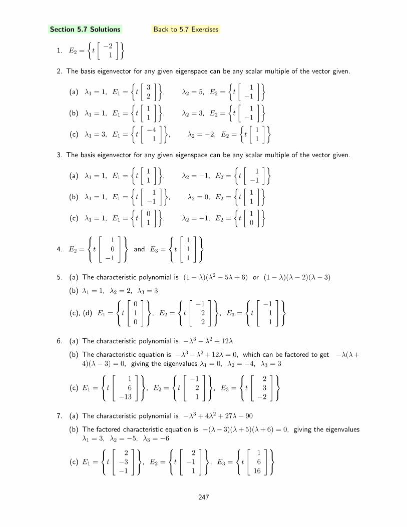
Section 5.7 Solutions Back to 5.7 Exercises
1. E2 =
t
[
−21
]
2. The basis eigenvector for any given eigenspace can be any scalar multiple of the vector given.
(a) λ1 = 1, E1 =
t
[
32
]
, λ2 = 5, E2 =
t
[
1−1
]
(b) λ1 = 1, E1 =
t
[
11
]
, λ2 = 3, E2 =
t
[
1−1
]
(c) λ1 = 3, E1 =
t
[
−41
]
, λ2 = −2, E2 =
t
[
11
]
3. The basis eigenvector for any given eigenspace can be any scalar multiple of the vector given.
(a) λ1 = 1, E1 =
t
[
11
]
, λ2 = −1, E2 =
t
[
1−1
]
(b) λ1 = 1, E1 =
t
[
1−1
]
, λ2 = 0, E2 =
t
[
11
]
(c) λ1 = 1, E1 =
t
[
01
]
, λ2 = −1, E2 =
t
[
10
]
4. E2 =
t
10−1
and E3 =
t
111
5. (a) The characteristic polynomial is (1− λ)(λ2 − 5λ+ 6) or (1− λ)(λ− 2)(λ− 3)
(b) λ1 = 1, λ2 = 2, λ3 = 3
(c), (d) E1 =
t
010
, E2 =
t
−122
, E3 =
t
−111
6. (a) The characteristic polynomial is −λ3 − λ2 + 12λ
(b) The characteristic equation is −λ3−λ2 +12λ = 0, which can be factored to get −λ(λ+4)(λ − 3) = 0, giving the eigenvalues λ1 = 0, λ2 = −4, λ3 = 3
(c) E1 =
t
16
−13
, E2 =
t
−121
, E3 =
t
23−2
7. (a) The characteristic polynomial is −λ3 + 4λ2 + 27λ− 90
(b) The factored characteristic equation is −(λ− 3)(λ+5)(λ+6) = 0, giving the eigenvaluesλ1 = 3, λ2 = −5, λ3 = −6
(c) E1 =
t
2−3−1
, E2 =
t
2−11
, E3 =
t
16
16
247

8. (a) The characteristic polynomial is −λ(1− λ)2
(b) λ1 = 0, λ2 = 1
(c) E1 =
t
130
, E2 =
s
010
+ t
201
9. λ1 = 1, E1 =
t
1−12
, λ2 = −2, E2 =
s
103
+ t
113
10. λ1 = 1, E1 =
t
110
, λ2 = 2, E2 =
t
001
11. See all rotated stress elements below the other answers.
(a) λ1 = 54.1,
x1=
[
4024.1
]
, λ2 = 25.9,
x2=
[
−404.1
]
, θ = tan−1 24.1
40= 31.1
(b) λ1 = −79.4,
x1=
[
45−19.4
]
, λ2 = 44.4,
x2=
[
45104.4
]
,
θ = tan−1 −19.445
= −23.3
(c) λ1 = 83.0,
x1=
[
20−3.0
]
, λ2 = −53.0,
x2=
[
20133.0
]
, θ = tan−1 −3.020
= −8.5
(d) λ1 = −116.1,
x1=
[
3576.1
]
, λ2 = −23.9,
x2=
[
−3516.1
]
, θ = tan−1 76.1
35= 65.3
ypxp
54.1 MPa
54.1 MPa
25.9MPa
25.9MPa
31.1
(a)
yp
xp
79.4 MPa
79.4 MPa
44.4MPa
44.4MPa
23.3
(b)
yp
xp
83.0 MPa
83.0 MPa
53.0MPa
53.0MPa
8.5
(c)
yp
xp
116.1MPa
116.1MPa
23.9 MPa
23.9 MPa
65.3
(d)
248