Linear Algebra for Computer Vision

Introduction

CMSC 828 D

Outline• Notation and Basics

• Motivation

• Linear systems of equations– Gauss Elimination, LU decomposition

• Linear Spaces and Operators– Addition, scalar multiplication, scalar product,

transformation, operator, basis

• Eigenvalues, Eigenvectors

• Solvability conditions (“alternative theorem”)– Adjoint, null space, orthogonality

Outline

• Euclidean space R3

– distance, angles, rotations

• Metric Space– Distance, angles, rotations

• Least Squares

• Singular Value Decomposition

• Other Matrix decompositions

Motivation• Fundamental to representation and numerical

solution of almost all problems including those in vision and computational statistics.– Solving equations for calibration, stereo, tracking, …

• Geometry is fundamental to vision. However one way of doing geometry is via algebra.– Intersections of lines, points, planes. Determining

angles. Determining orthogonal projections …

• Modern computer vision is formulated in terms of “projective geometry”. Most results in projective geometry are stated algebraically and require knowledge of concepts such as rank, null space, constraints

Applications

• Rectification of images

• Calibrating cameras

• Transforming color spaces

• Tracking motion of a rigid body

• Applying constraints from multiple views

• Parametrizing fundamental matrix and trifocal tensor.

Vectors• A vector x of dimension d represents a point in a d

dimensional space• Examples

– A point in 3D Euclidean space [x,y,z] or 2D image space [u,v]– A point in a projective space P3 [X,Y,Z,W] or in projective space

P2 [U,V,W]– Point in color space [r,g,b] or [y, u, v]– Point in an infinite dimensional functional space on a Fourier

basis– Vector of intrinsic parameters for a camera (focal length, skew

ratio, …)

• Essentially a short-hand notation to denote a grouping of points – No special structure yet

Vectors and Matrices

• d×n dimensional matrix M and its transpose Mt

• Transpose indicated with a superscript t or a prime ′

•d dimensional column vector x and its transpose

Determinant• Determinant of a 2x2 matrix m11m22-m12m21

• For a higher dimensional matrix we have a recursive definition

Determinant: Remarks

• Determinant determines “magnitude” of matrix. Matrix with determinant =0 is called singular.

• Determinant is important in theorems• Practically the way to compute the

determinant is not this way.• Homework problem -- determine number of

operations for recursive algorithm.

Matrix basics

• Square matrix: number of rows = number of columns

• Symmetric matrix Aij=Aji .

• Skew symmetric matrix Aij=-Aji .

• Identity I ij= δij

– Kronecker delta δij=0 if i≠j δij=1 if i=j

• Lower triangular Upper triangular0 0

0

0

0 0

a a c d

c b b

e

f g d d

" "

% # % #

# " % # % %

" "

Matrix vector product

• m×n dimensional matrix M multiplies by a n dimensional vector x to produce a m dimensional vector

Linear systems of equations

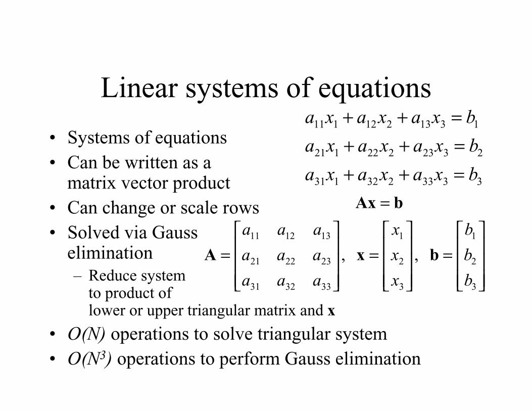
• Systems of equations• Can be written as a

matrix vector product• Can change or scale rows• Solved via Gauss

elimination– Reduce system

to product of lower or upper triangular matrix and x

• O(N) operations to solve triangular system• O(N3) operations to perform Gauss elimination

11 1 12 2 13 3 1

21 1 22 2 23 3 2

31 1 32 2 33 3 3

a x a x a x b

a x a x a x b

a x a x a x b

+ + =+ + =+ + =

11 12 13 1 1

21 22 23 2 2

31 32 33 3 3

, ,

a a a x b

a a a x b

a a a x b

=

= = =

Ax b

A x b

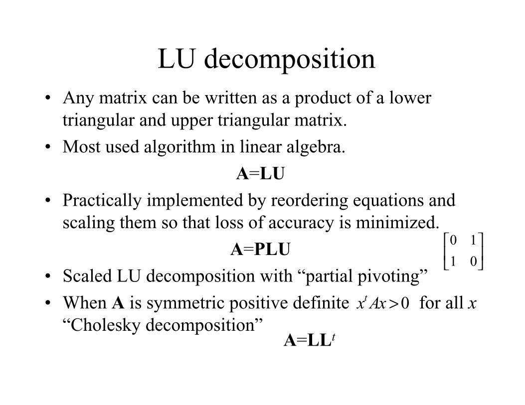
LU decomposition• Any matrix can be written as a product of a lower

triangular and upper triangular matrix.

• Most used algorithm in linear algebra.

A=LU

• Practically implemented by reordering equations and scaling them so that loss of accuracy is minimized.

A=PLU

• Scaled LU decomposition with “partial pivoting”

• When A is symmetric positive definite for all x“Cholesky decomposition”

A=LLt

0 1

1 0

0tx Ax >

Linear/Vector Spaces• Previous stuff was somewhat mechanical.• In vision we have to answer questions when

– Models provide equations that are singular or degenerate. What can we say about the solutions? Can we restrict them?

– Number of unknowns may be more or less than the number of observations. Can we still obtain a meaningful solution?

– How “far” is an approximation from a solution? How do we measure this distance?

– Matrices are operators that take one vector into another. What can we say about the properties of the operator? When is an equation involving an operator solvable?

Operators

• Function, Transformation, Operator, Mapping: synonyms

• A function takes elements x defined on its “Domain” D to elements y in its “Range” R which is part of E

• If for each y in R there is exactly one x in D the function is one-to-one. In this case an inverse exists whose domain is R and whose range is D

• We are interested in situations where R and D are finite-dimensional linear spaces

D

E

R

Vector Space• A collection of points that obey certain rules

– Commutative, existence of a zero element

– Scalar multiplication

• Let u1, …, uk be a set of vectors:Linear combination

( ); ( ) ( )

0, 0 ; 0

u v v u u v w u v w

u u u u u

+ = + + + = + +∃ + = ∀ + − =

( ) ( )( ) ( )

; 1

;

u u u u

u u u u v u v

α β αβ

α β α β α α α

= =

+ = + + = +O

u

2u

-u

v

u+v

Manifold spanned by u1 1 k kα α+ +u u"

Dependence and dimensionality• A set of vectors is dependent if for some scalars α1, …, αk not

all zero we can write• Otherwise the vectors are independent.• If the zero vector is part of a set of vectors that set is

dependent. If a set of vectors is dependent so is any larger setwhich contains it.

• A linear space is n dimensional if it possesses a set of n independent vectors but every n+1 dimensional set is dependent.

• A set of vectors b1, …, bk is a basis for a k dimensional space X if each vector in X can be expressed in one and only one way as a linear combination of b1, …, bk

• One example of a basis are the vectors (1,0,…,0), (0,1,…,0), …, (0,0, …, 1)

1 1 0k kα α+ + =u u"

Distances/Metrics and Norms• We would like to measure distances and directions in the

vector space the same way that we do it in Euclidean 3D

• Distance function d(u,v) makes a vector space a metric space if it satisfies– d(u,v)>0 for u,v different

– d(u,u)=0, d(u,v)=d(v,u)

– d(u,w)≤ d(u,v)+d(v,w) (triangle inequality)

• Norm (“length”). – ||u|| >0 for u not 0, ||0||=0

– || α u||=| α| ||u||, ||u+v || ≤ ||u|| + ||v||

• Normed linear space is a metric space with the metric defined by d(u,v)=||u-v|| and ||u||=d(u,0)

• Dot product of two vectors with same dimension<x,y> =

• Dot product space behaves like Euclidean R3

• Dot product defines a norm and a metric.• Parallelogram law

||u+v||2+||u-v||2 = 2||u||2 + 2 ||v||2

• Orthogonal vectors <u,v>=0• Angle between vectors

cos θ=<x,y>/||x|| ||y||

• Orthonormal basis -- elements have norm 1 and are perpendicular to each other

• Other distances and products can also define a space:– Mahalnobis distance

Dot Product

Matrices as operators• Matrix is an operator that takes a vector to

another vector.– Square matrix takes it to a vector in the space of

the same dimension.

• Dot product provides a tool to examine matrix properties– Adjoint matrix < Au,v> = <u,A*v>– Square Matrix fully defined as result of its

operation on members of a basis.Aij = < Abj,bi>

Eigenvalues and Eigenvectors• Square matrix possesses its own natural basis.• Eigen relation

Au=λu• Matrix A acts on vector u and produces a scaled version of

the vector.• Eigen is a German word meaning “proper” or “specific”• u is the eigenvector while λ is the eigenvalue.

– If u is an eigenvector so is αu – If ||u||=1 then we call it a normal eigenvector– λ is like a measure of the “strength” of A in the direction of u

• Set of all eigenvalues and eigenvectors of A is called the “spectrum of A”

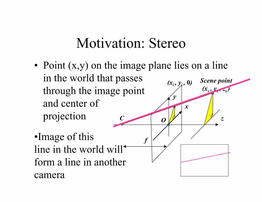
Motivation: Stereo

• Point (x,y) on the image plane lies on a line in the world that passes through the image pointand center of projection C

Scene point(xs , ys , zs )

(xi , yi , 0)

x

z

y

f

O

•Image of thisline in the world willform a line in another camera

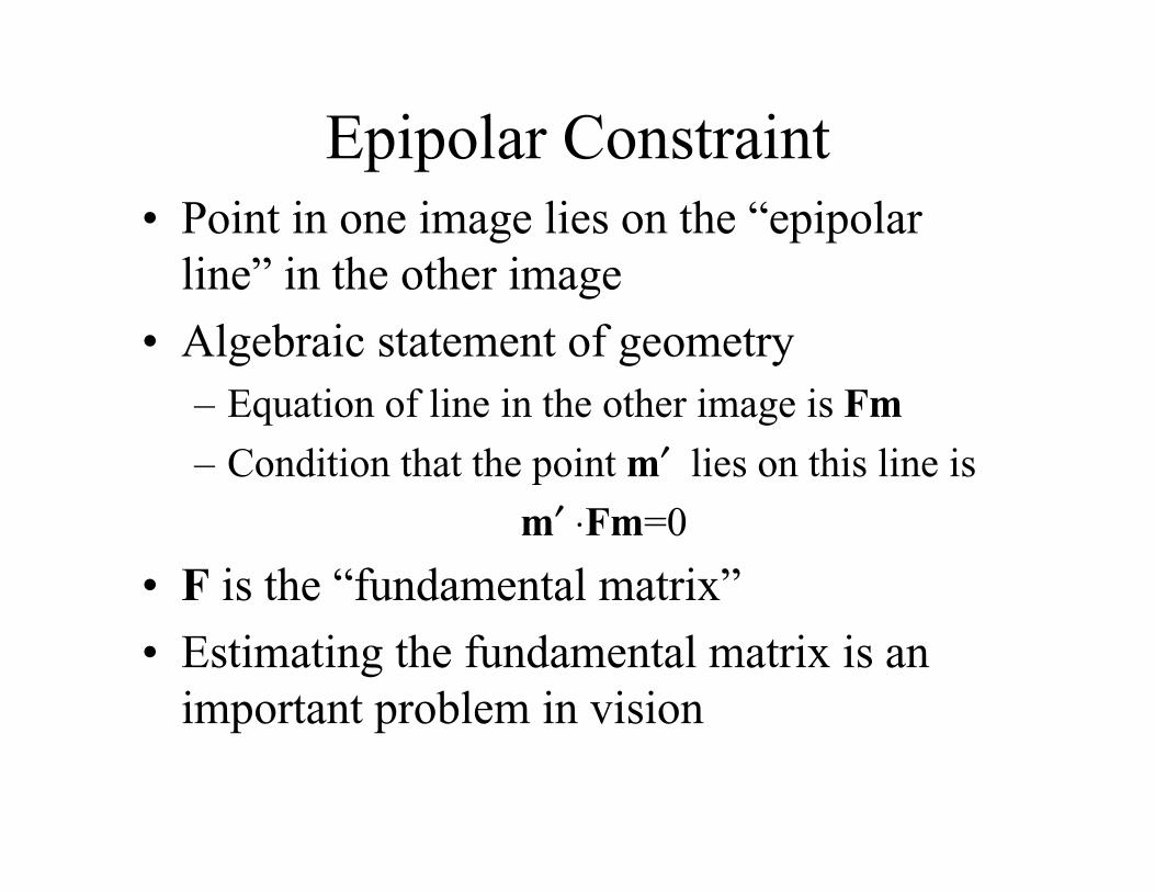
Epipolar Constraint• Point in one image lies on the “epipolar

line” in the other image

• Algebraic statement of geometry– Equation of line in the other image is Fm

– Condition that the point m′ lies on this line is

m′ ⋅Fm=0

• F is the “fundamental matrix”

• Estimating the fundamental matrix is an important problem in vision

Eight point algorithm: Determining the Fundamental matrix

• Given a set of matching points in the images, Determine F

0i j ijm m F =∑

[ ]

( ) ( ) ( )11 12 13 21 22 23 31 32

1 0

1

1 0

11 12 13

21 22 23

31 32 1

u

u v v

u f u f v f v f u f v f f f

f f f

f f f

f f

′ ′ =

′ ′+ + + + + + + + =

Determining F

• Write expression as an equation in the unknown elements.

• If we have eight points we can solve for elements of F, (e.g. via LU)

• If we have more than eight pointswe can use a least squares formulation

[ ] [ ]

11

12

13

21

22

23

31

32

1 1 1

f

f

f

fu u u v u v u v v v

f

f

f

f

′ ′ ′ ′ ′ ′ = −