Limits and Derivatives2

What Does f Say About f ?2.8

3

What Does f Say About f ?Many of the applications of calculus depend on our ability to deduce facts about a function f from information concerning its derivatives.

Because f (x) represents the slope of the curve y = f (x) at the point (x, f (x)), it tells us the direction in which the curve proceeds at each point.

So it is reasonable to expect that information about f (x) will provide us with information about f (x).

4

What Does f Say About f ?In particular, to see how the derivative of f can tell us where a function is increasing or decreasing, look at Figure 1.

Between A and B and between C and D, the tangent lines have positive slope and so f (x) > 0.

Between B and C, the tangent lines have negative slope and so f (x) < 0.

Thus it appears that f increases when f (x) is positive and

decreases when f (x) is negative.

Figure 1

5

What Does f Say About f ?

It turns out that what we observed for the function graphed

in Figure 1 is always true. We state the general result as

follows.

6

Example 1 – Given a Graph of f , What Does f Look Like?

(a) If it is known that the graph of the derivative f of a function is as shown in Figure 2, what can we say about f ?

(b) If it is known that f (0) = 0, sketch a possible graph of f.

Figure 2

7

Example 1(a) – Solution

We observe from Figure 2 that f (x) is negative when

–1 < x < 1, so the original function f must be decreasing on

the interval (–1, 1).

Similarly, f (x) is positive for x < –1 and for x > 1, so f is

increasing on the intervals (– , –1) and (1, ).

Also note that, since f (–1) = 0 and f (1) = 0, the graph of f

has horizontal tangents when x = 1.

8

Example 1(b) – SolutionWe use the information from part (a), and the fact that the graph passes through the origin, to sketch a possible graph of f in Figure 3.

Notice that f (0) = –1, so we have drawn the curve y = f (x) passing through the origin with a slope of –1.

Figure 3

cont’d

9

Example 1(b) – SolutionNotice also that f (x) 1 as x (from Figure 2).

So the slope of the curve y = f (x) approaches 1 as x becomes large (positive or negative).

That is why we have drawn the graph of f in Figure 3 progressively straighter as x .

Figure 2

cont’d

10

What Does f Say About f ?

We say that the function f in Example 1 has a local

maximum at –1 because near x = –1 the values of f (x) are

at least as big as the neighboring values.

Note that f (x) is positive to the left of –1 and negative just to

the right of –1.

Similarly, f has a local minimum at 1, where the derivative

changes from negative to positive.

11

What Does f Say About f ?

12

What Does f Say About f ?

Let’s see how the sign of f (x) affects the appearance of the

graph of f.

Since f = (f ), we know that if f (x) is positive, then f is

an increasing function.

This says that the slopes of the tangent lines of the curve

y = f (x) increase from left to right.

13

What Does f Say About f ?Figure 4 shows the graph of such a function.

The slope of this curve becomes progressively larger as x increases and we observe that, as a consequence, the curve bends upward. Such a curve is called concave upward.

Figure 4

Since f (x) > 0, the slopes increaseand f is concave upward.

14

What Does f Say About f ?In Figure 5, however, f (x) is negative, which means that f is decreasing.

Thus the slopes of f decrease from left to right and the curve bends downward. This curve is called concave downward.

Figure 5

Since f (x) < 0, the slopes decreaseand f is concave downward.

15

What Does f Say About f ?We summarize our discussion as follows.

16

Example 2Figure 6 shows a population graph for Cyprian honeybees raised in an apiary. How does the rate of population increase change over time? When is this rate highest? Over what intervals is P concave upward or concave downward?

Figure 5

17

Example 2 – Solution By looking at the slope of the curve as t increases, we see that the rate of increase of the population is initially very small, then gets larger until it reaches a maximum at about t = 12 weeks, and decreases as the population begins to level off.

As the population approaches its maximum value of about 75,000 (called the carrying capacity), the rate of increase, P (t), approaches 0.

The curve appears to be concave upward on (0, 12) and concave downward on (12, 18).

18

What Does f Say About f ?In Example 2, the population curve changed from concave upward to concave downward at approximately the point (12, 38,000).

This point is called an inflection point of the curve.

The significance of this point is that the rate of population increase has its maximum value there.

In general, an inflection point is a point where a curve changes its direction of concavity.

19

Antiderivatives

20

Antiderivatives

In many problems in mathematics and its applications, we

are given a function f and we are required to find a function

F whose derivative is f.

If such a function F exists, we call it an antiderivative of f.

In other words, an antiderivative of f is a function F such

that F = f. (In Example 1 we sketched an antiderivative f of

the function f .)

21

Example 4 – Sketching an Antiderivative

Let F be an antiderivative of the function f whose graph is shown in Figure 8.

(a) Where is F increasing or decreasing?

(b) Where is F concave upward or concave downward?

(c) At what values of x does F have an inflection point?

(d) If F(0) = 1, sketch the graph of F.

(e) How many antiderivatives does f have?

Figure 8

22

Example 4 – Solution(a) We see from Figure 8 that f (x) > 0 for all x > 0. Since F is

an antiderivative of f, we have F (x) = f (x) and so F (x) is positive when x > 0.

This means that F is increasing on (0, ).

(b) F is concave upward when F (x) > 0. But F (x) = f (x), so F is concave upward when f (x) > 0, that is, when f is increasing. From Figure 8 we see that f is increasing when 0 < x < 1 and when x > 3.

So F is concave upward on (0, 1) and (3, ).

23

Example 4 – Solution F is concave downward when F (x) = f (x) < 0, that is,

when f is decreasing.

So F is concave downward on (1, 3).

(c) F has an inflection point when the direction of concavity changes. From part (b) we know that F changes from concave upward to concave downward at x = 1, so F has an inflection point there.

F changes from concave downward to concave upward when x = 3, so F has another inflection point when x = 3.

cont’d

24

Example 4 – Solution

(d) In sketching the graph of F, we use the information from

parts (a), (b), and (c).

But, for finer detail, we also bear in mind the meaning of

an antiderivative: Because F (x) = f (x), the slope of

y = F (x) at any value of x is equal to the height of

y = f (x).

cont’d

25

Example 4 – Solution Therefore, since f (0) = 0, we start drawing the graph of F

at the given point (0, 1) with slope 0, always increasing, with upward concavity to x = 1, downward concavity to x = 3, and upward concavity when x > 3. (See Figure 9.)

cont’d

Figure 9

An antiderivative of f

26

Example 4 – Solution

Notice that f (3) ≈ 0.2, so y = F (x) has a gentle slope at

the second inflection point. But we see that the slope

becomes steeper when x > 3.

(e) The antiderivative of f that we sketched in Figure 9

satisfies F(0) = 1, so its graph starts at the point (0, 1).

But there are many other antiderivatives, whose graphs

start at other points on the y-axis.

cont’d

27

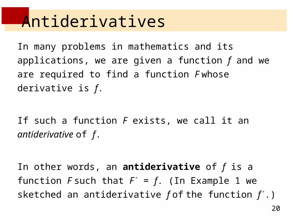
Example 4 – Solution In fact, f has infinitely many antiderivatives; their graphs

are obtained from the graph of F by shifting upward or downward as in Figure 10.

cont’d

Figure 10

Members of the family ofantiderivatives of f