Limited Food Access as an Equilibrium Outcome: An Empirical Analysis

Alessandro Bonanno Assistant Professor of Agricultural Economics

Department of Agricultural Economics and Rural Sociology The Pennsylvania State University

207-D Armsby Building University Park, PA16802 USA

Tel: (814) 863-8633 Fax: (814) 865 3746

Email: abonanno@psu.edu

Lauren Chenarides Ph.D. Student in Agricultural, Environmental, and Regional Economics

Department of Agricultural Economics and Rural Sociology The Pennsylvania State University

308 Armsby Building University Park, PA 16802-5600

and

Stephan J. Goetz

Director, The Northeast Regional Center for Rural Development Professor of Agricultural and Regional Economics

The Pennsylvania State University 207-C Armsby Building,

University Park, PA 16802 USA Phone: 814/863-4656

e-mail: sgoetz@psu.edu; http://nercrd.psu.edu Selected Paper for the joint AAEA and EAAE Symposium: “Food Environment: The Effects of Context on Food Choice.” Tufts University, Boston, MA, May 30–31, 2012. Acknowledgements: The authors gratefully acknowledge funding from USDA/NIFA under Global Food Security Grant No. 2011-68004-30057 (Enhancing the Food Security of Underserved Populations in the Northeast U.S. through Sustainable Regional Food Systems Development) and the Agricultural Experiment Station of The Pennsylvania State University; any opinions are strictly those of the authors.

Limited Food Access as an Equilibrium Outcome: An Empirical Analysis

Abstract

Lack of access to nutritious and affordable food has become an important public policy issue in the U.S.: various interest groups are seeking to reverse a trend whereby certain areas lack larger, full-service grocery stores that provide “higher” quality foods. Based on game-theoretic findings suggesting that lack of food access can be an equilibrium outcome, we specify a model relating access to higher quality food stores to a vector of supply and demand factors, using seven years of county-level data for the contiguous U.S., and a constrained generalized ordered logit estimator. Our results suggest that demand side factors, especially market size (total income and SNAP funds) play an important role in determining food access, and that large food stores avoid areas with higher poverty. Some cost determinants, such as the ratio of building costs to the total site cost, home price index (for counties with higher poverty rates than the average) and ease of recruiting labor, affect the probability of observing areas with no access. A more favorable business tax regime has no impact on access, while better transportation infrastructure reduces rather than improves food access. Our results shed new light on the determinants of food access in addition to highlighting what policy can and cannot accomplish to improve food access.

JEL Codes: Q18; R3; L81

Key Words: Food Access, Equilibrium; Food-Store Density

Limited Food Access as an Equilibrium Outcome: An Empirical Analysis

The relationship between consumer diets and characteristics of the “food environment”1

has been widely investigated and is the object of considerable policy debate because of its

profound implications for consumer well-being, especially those with low incomes (inter alia

Hawkes 2008; Holsten 2007). Copious evidence suggests that areas inhabited predominantly by

less-privileged individuals are characterized by fewer large (or “high quality”) food stores (see,

inter alia, Alwitt and Donley 1997; Ball, Timperio and Crawford 2008; Morland, Wing and Diez

Roux 2002; King, Leibtag, and Behl 2004; Moore and Diez Roux 2006; Powell et al. 2007; Zenk

et al. 2005), and that limited access to food stores can constitute a barrier to obtaining adequate

amounts of nutritious food (Haering and Syed 2009; Ver Ploeg et al. 2009). A positive

relationship exists between the quality of food choices available to low-income (food stamp

recipient) households and access to food outlets (Rose and Richards 2004) and by the same

token, empirical evidence suggests that richer food environments lead to lower levels of food

insecurity (Bonanno and Li 2011). Also, a relationship between access to different types of food

outlets and obesity has been argued to exist both in the U.S. and internationally (Morland, Diez

Roux and Wing 2006; Hawkes 2008; White 2007).

The term “food desert” has been minted to describe the likely negative relationship

between diminished food access and ability to maintain a healthy diet; in the 2008 Farm Bill the

U.S. government defines these as areas “… with limited access to affordable and nutritious food,

particularly […] composed of lower-income neighborhoods and communities” (for other

definitions see Ver Ploeg et al. 2009). Identifying and measuring food deserts is complex and

depends on which food stores should be considered, what the definition of “neighborhoods and 1The food environment comprises all factors influencing the availability of, or consumers’ access to, food that can be consumed at home (food-at-home) and ready-to-eat pre-cooked food for consumption away from home (food-away-from-home) (Cummins and Macintyre 2006).

communities” is, and what “affordable” and “nutritious” food means (see Ver Ploeg et al. 2009

for further considerations).

The concept of food desert as illustrated above links the supply of nutritious food

products (and by default, of food outlets providing them) to low-income consumers, and the cost

they face in obtaining such products. Although larger stores2 belonging to organized chains can

achieve lower costs by using their efficiency along the supply chain and offer healthier food (i.e.,

fruit and vegetables) at lower price than smaller, unorganized stores (Hawkes 2008), empirical

evidence on whether the presence of larger stores selling healthier products improves consumer

diets is mixed. For example, while Rose and Richards (2004) found that ease of supermarket

access is associated with increased daily consumption of fruits and vegetables among food stamp

recipients, Cummins et al. (2005) found no significant changes in consumption habits after entry

of a large-scale food retailer.

Although the interaction between the healthfulness of low-income consumer choices and

the food environment is complex (Drewnowski and Darmon 2005) the drivers of the supply-side

component of food deserts can be inferred using simple economic principles. Bitler and Haider

(2011) point out that the existence of areas characterized by limited food access can be

rationalized in an economic framework by referring to the interaction of demand and supply

drivers. Assuming that nutritious food is a normal good, demand for it will increase with

income; thus, demand for stores providing such food will be lower in low-income areas. Also

differences in taste (which may be related to educational level, ethnicity, etc…) may lead to

varying demand for “healthy” foods. The supply-side of the issue, on the other hand, instead

2 In general terms, limited access to “large” food stores may result in higher search and transportation costs and lead to higher food prices because of monopoly power or cost inefficiencies characteristic of smaller stores (King, Leibtag, and Behl 2004). Limited access could cause further hardships for low-income consumers who may lack adequate transportation means and have limited ability to adopt cost-saving strategies (Leibtag and Kaufman 2003).

relates to the costs of investment and operation facing food outlets in terms of sourcing, sorting

and distributing foods. Even under perfect competition (as Bitler and Haider argue), a shrinking

demand curve could intersect the long-run average cost of retailing food in its downward-sloping

portion, indicating long-run downward sloping supply, i.e., a reduction in the number of stores.

However, perfect competition does not apply to modern food retailers, who offer retailing

services that cannot be separated from the physical products sold in the stores (Betancourt and

Gautschi 1988, 1993; Bonanno and Lopez 2009); that is, retail food represents a bundle of

differentiated products comprised of the physical product, services, ambience and assortments

(Betancourt and Gautschi 1990, 1993; Betancourt 2006; Richards and Hamilton 2006; Bonanno

and Lopez 2009). Some food retailers invest in fixed cost to increase their overall “quality”

level, softening price competition to become more attractive to consumers who are less price-

sensitive (Bonanno and Lopez 2009); thus fixed costs are endogenously determined (Sutton

1991).3 The existence of high fixed costs and consumer heterogeneity across markets may lead

both firms and consumers to sort according to their features – i.e., costs and preferences – which

lead some goods not to be available in all markets (Waldfogel 2008). In sum, these factors,

suggest that limited access to nutritious food for low-income consumers may simply be an

equilibrium outcome of differentiated product firms (i.e., food retailers) selling their products

(i.e., locating their stores) in markets where there is a sizable demand. Such firms will play a

multi-stage game while facing consumers who are heterogeneous across markets (i.e., income

levels and taste for “quality” change across areas but all consumers in the same market are

assumed to be identical).

3 This rationale, which follows Sutton’s (1991) endogenous cost model, is used by Ellickson (2006, 2007) to explain how the food retailing industry has become a two-tiered industry where a large firm of smaller (low-quality) stores coexists with a natural oligopoly of fewer, large (high-quality) firms.

In this paper we consider an empirical framework where both demand and supply-side

factors determine access to large food outlets (grocery stores with more than 50 employees and

Walmart Supercenters). We measure the extent of access via a Limited Access Index (LAI)

obtained by dividing the number of large stores in a county by a number of partitions consistent

with pre-specified potential area of influence for a store (10 miles radius in rural counties and 0.5

miles in urban ones). Our results suggest that although the role of demand-side factors outweighs

supply-side forces in determining lack of access, policy seeking to improve access, especially in

areas with more low-income households, needs to consider both aspects.

The Model

What follows describes the strategic game in Ellickson (2006, 2007), which uses the

Endogenous Sunk Cost framework developed by Sutton (Shaked and Sutton 1987; Sutton 1991).

Consumers in a given market j are identical and value retail quality (i.e., food retailers represent

vertically differentiated goods). Food retailers play a three-stage game: in the first stage both

potential entrants and incumbent stores decide whether or not to enter market j (incumbents

playing “Enter” when they do not exit the market); in the second stage firms that have entered

set the level of quality offered to consumers (i.e., assortment and level of service, as in Bonanno

and Lopez 2009); in the third stage firms compete à la Cournot. Of the two types of stores

considered in Ellickson (2006, 2007) we focus only on those offering “high quality,” which are

characterized by large assortments and food products likely to be of high quality.

Assume symmetric demand and cost, and let the observed number of firms in market j

represent a possible equilibrium of this game (Bresnahan and Reiss 1991; Berry 1992); define

this equilibrium number of firm as*jN .4 If, in a given market, none of the potential entrants finds

it optimal to play “enter” or, in other words “do not enter” represents the best response to any of

the other players’ actions, the equilibrium number of large food retail firms in j is *jN =0; in that

case consumers in j will be deprived of access to large food outlets. Ellickson (2007) shows that,

for high quality stores, *jN depend on market size, investment costs (in his paper price of land)

and the relative costliness of investing in quality to satisfy quality-valuing consumers. He

presents three possible scenarios: 1) the equilibrium number of firms increases with market size;

2) the equilibrium number of firms decrease as market size expands (i.e., a market can become

saturated), an effect reinforced by increasing investment costs; and 3) if the market size is small,

corner solutions are possible where*jN ≤1. This last outcome explains the lack of large stores, at

least in some markets.5

We observe the number of firms in geographic areas (indexed by l =(1,...,L)) which are

aggregates of smaller local markets each representing a suitable location for a food retail store. In

each area l the number of these markets represents the number of partitions into which l can be

broken (i.e., each partition represents a potential market of interest). Let the number of markets

in area l be indexed by jl (j=(1,…,Jl), and the number of partition by Mktl. The average number

of (equilibrium) retail firms in a market in l is given by * *l jl l

j l

N N Mkt∈

=∑ where *jl

j l

N∈∑ is the

4 Entry games usually have multiple equilibria. Sorting firms (facing symmetric demand and cost) by decreasing profitability (i.e., the most profitable firms enter the market first, as in Bresnahan and Reiss 1991; and Berry 1992) the observed number of market participants is one Nash equilibrium of such a game. We abstract from the dynamic aspects of entry games as this is outside the scope of this work (see Jia (2008) for an example). 5 In its empirical application, Ellickson (2006) shows that in the U.S. food retailing industry the second scenario (N*

j decreasing with market size) is the most likely to be observed for large stores. He finds that while low-quality, smaller stores have an equilibrium number of firms increasing with market size, higher-quality stores, investing in fixed costs, organize in a natural oligopoly where the equilibrium number of firms does not grow indefinitely with market size. Similar notions apply to other industries where firms commit to a specific location (see for example Asplund and Sandin’s (1999) application to Swedish regional markets for driving schools).

equilibrium number of large food retail firms in l. Assume the following relationship explains*lN

:

* ln ( ; ) ( ; )D Cl l l lN S g gα ε= + + +D C

l lX α C ,K α

(1)

where l jl lj l

S S Mkt∈

=∑ , jlS being the size of each market j in area l , measured by total income

and ln() is the natural log operator (consistent with Ellickson (2006) who indicated that the

equilibrium number of high quality firm declines with market size); gD(.) and gC(.) are functions

qualifying, respectively, how demand (other than market size) and cost factors affect the

equilibrium number of firms; Xl is a vector of demand shifters (including also an average

measure of the composition of consumers across the j markets in l to account for heterogeneity

across areas); Cl and K l are vectors of variables capturing, respectively, variable and fixed cost;

αD and αC are conformable vectors of parameter; and εj is a random term capturing other

(unobserved) factors which could impact firm locations *lN .

Under the assumptions of footnote 4, the observed average number of firms in each

partition represents an equilibrium. *lN then serves as an indicator of consumers’ access to large

food retailers. First, outcome *lN =0 represents a scenario where no firm finds it profitable to

locate in any of the partitions of l (no access); second, *0 < 1lN < indicates that, on average, at

least one of the markets in l will have no large food retailer (limited access); and last, if * 1lN ≥

all markets in l have, on average, at least one large food store (adequate access). Using this

categorization, we define the Limited Access Index (LAI) as

*

*

*

0 if 1;

1 if 0 < 1; (2)

2 if 0;

l

l l

l

N

LAI N

N

≥= < =

Let h = {0,1,2} be one of the three possible outcomes of LAI; assume that gD(.) and gC(.)

are linear in variables and parameters and let Zl = [ln lS , Xl, Cl , K l ] contain the covariates in

(1) and θ = [α, αD , αC ] represent its parameters. Then the probability that a given outcome of

LAI conditional on both the demand and cost factors is observed is:

Pr(LAIl =h| Zl) = Λ (δ h -1 – Zl`θ) – Λ (δ h – Zl`θ); (3)

where Λ is the logistic CDF, δ0 = –∞, δ3 = +∞ (δ1 and δ2 represent “cut-off” points) so that the

vector of coefficients θ can be estimated via maximum likelihood ordered logit. More details on

the estimation method are provided in the next section.

Data and Estimation

We estimate equation (3) using seven years (2000-2006) of observations for 2,876

contiguous U.S. counties, comprised of 20,132 observations. For our definition of access to

large food stores, we adopt an approach similar to that in Ver Ploeg et al (2009). The county-

level number of large food retailers is the sum of grocery store establishments (NAICS 44511 >

50 employees) from the County Business Patterns, plus the number of Walmart Supercenters

from T.J. Holmes’ database (Holmes 2010, 2011). Dividing this number by the square miles of

land in each county, obtained from the U.S. Bureau of Census Gazetteer of counties (2001)

rescaled to account for the potential travel radius to reach a store (Ver Ploeg et al. 2009, box b1),

i.e., 10 miles radius in rural counties and 0.5 miles in urban ones (identified via the USDA Rural-

Urban continuum codes), we obtain a county-level Limited Access Index.

As noted above we include demand and supply side variables that could impact store

location decisions. The demand-side variables capture market potential and heterogeneity in taste

across areas. Among the first group of variables we include a proxy for total market size (log of

total income, from the Bureau of Economic Analysis); population density, calculated in

thousands of people per square mile (from the U.S. Census Bureau Population Estimates

Program – PEP); poverty rate (from the Small Area Income and Poverty Estimates – SAIPE – by

the U.S. Bureau of Census), to represent demand limitations; and a variable capturing the

additional potential demand coming from low-income individuals who participate in the

Supplemental Nutrition Assistance Program (SNAP) measured as SNAP participants/ population

in poverty (both from SAIPE). Variables capturing consumers’ heterogeneity across areas are the

share of population that is black, Hispanic, and 14-25 years of age, 25-64 years of age, and over

65 (from the PEP).

Supply-side determinants aim to capture two types of costs: fixed investment (and

location) costs and operating costs. Fixed cost variables are state-level variables measuring the

ratio of the cost of the structure to the total value of a home, i.e. the “structure share” and a home

price Index from the “Land Prices by State” database of the Lincoln Institute of Land Policy as

described in Morris and Heathcote (2007); share of non-agricultural land from the USDA

National Agricultural Statistical Service (to proxy for land availability). As for the sources of

variable costs, we consider the following: large stores require more frequent delivery of goods

and may operate their own truck fleet, and so we include the “on-highway” price of diesel (all

types) in $/gal (from the U.S. Department of Energy); another common cost in retailing is

electricity: we include monthly retail prices of electricity for commercial use ($/Kwh), also from

the U.S. Department of Energy. Although labor is another major cost in retailing, we excluded

proxies for retail wages as they are impacted by the composition of the local retail industry;

instead we used county-level unemployment rates (from the Local Area Unemployment

Statistics, the U.S. Bureau of Labor Statistics) to capture the ease with which unskilled retail

workers can be recruited.

Additional controls added to the model are: ease of distribution/capillarity of

infrastructure, i.e., state-level miles of public roads/squared miles of land (U.S. Department of

Transportation, Federal Highway Administration); the likelihood of benefiting from “short”

channels, via the share of vegetables produced in each acre of agricultural land in a county (from

the USDA National Agricultural Statistical Service); the presence of a “business friendly” tax

regimes, via an indicator variable that identifies states with zero corporate income taxes (from

the U.S. Tax Foundation), an indicator variable for Metropolitan areas (calculated from the

USDA Rural-Urban continuum codes); and, lastly, as the LAI contains the number of Walmart

Supercenters, the distance from Benton County, Arkansas, to capture part of the chain’s hub-&-

spoke logistics system (Courtemanche and Carden 2011; Bonanno 2010). This is obtained by

applying the Haversine formula to county centroid coordinates (U.S. Bureau of Census Gazetteer

of Counties 2001). State-level fixed effects and year dummies are also included in the model.

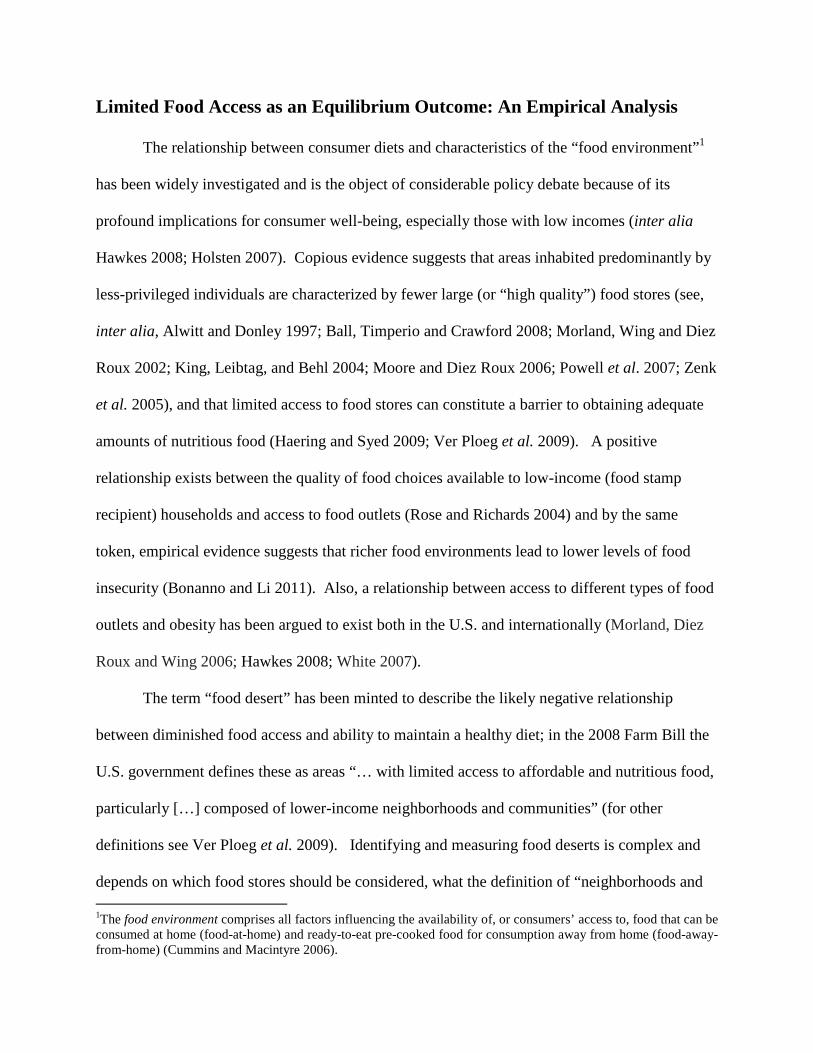
A list of variables and their summary statistics is provided in Table 1, which also

illustrates some of the differences across areas showing different values of LAI. From the data it

emerges that 23.8% (4,791) of the counties considered had no large food store, while a slightly

smaller proportion of counties showed LAI of 0 (full coverage by large food stores, 21.3%). One

of the most striking features of the data is the difference across subsamples of counties

characterized by “no access” (LAI=2) or “limited access” (LAI=1) and those with “adequate

access”. In particular, counties characterized by LAI=2 show some an aging population (lower

share of population between 15-24 years of age and higher share of over 65), larger shares of

Hispanic population, higher poverty rates, but also higher rates of SNAP redemptions, lower

population density, smaller market size (i.e. lower levels of ln(INC)). Also, as one can see from

the values at the bottom of table 1, a disproportionally large share of counties LAI=2 are located

in the South or Midwest.6

With respect to the proxies for fixed cost, the average value of the share of structure cost

over the total cost of buildings is higher in “no access” areas than the average suggesting that,

relatively speaking, building larger stores may be more expensive in these areas. However, the

home price index does not show large variations across areas with different LAI. As for the

variable costs, while electricity for commercial use is on average cheaper in areas characterized

by LAI=2, the price of diesel shows little variation, while unemployment rates are lower. Not

surprisingly the quality of the infrastructure is worse in areas characterized by less access (i.e.,

the number of miles of highways per square mile is lower) while the share of agricultural land is

higher. Lastly, the average distance from Benton County in “no access” areas is lower, and there

also are more areas without corporate income tax, consistent with the fact that 50% of these

counties are located in the South.

Moving on to an illustration of the estimation method used, as mentioned above, equation

(3) is estimated via ordered logit. However, the parameters of the ordered logit are constrained to

satisfy the proportional odds assumption, which can be restrictive if the independent variables

impact the different levels of LAI in a non-proportional way. To relax these restrictions, the

model was re-estimated via a constrained generalized ordered-logit which allows, via a backward

stepwise selection process, to impose sequential constraints on the estimated coefficients that do

not violate the proportional odds property, leaving the other coefficients unconstrained (Long

and Freese 2006; Williams 2006). Wald-tests on the estimated parameters did not support the

6 Some of these features are similar to those characterizing food deserts in rural counties described in Morton and Blanchard (2007).

rejection of the null that the parameters jointly satisfy the proportional odds assumption. Data

manipulation and estimation were performed in STATA version 11.

Empirical Results and Discussion

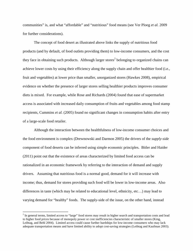
The estimated parameters of equation 3, reported in table 2, were obtained using different

estimators: ordered logit (first column; OL) constrained generalized ordered logit (second and

third columns; CGOL), and a generalized ordered logit (last two columns; GOL). The values of

the pseudo R squared show CGOL and GOL outperforming OL; the use of either of the first two

estimators leads to very little difference in goodness of fit with values of the pseudo R squared

being, respectively, 0.5474 and 0.5478 while the OL has only limited explanatory power.

Furthermore, the p-value of a Wald test for the validity of the parallel regression assumption

(under the null of the regression curves’ slopes being jointly the same) performed on the OL

coefficients is 0.000, indicating that the parallel regression assumption is not satisfied. The step-

wise sequential process of the CGOL shows that for 19 parameters the parallel regression

assumption holds (for these parameters the null of the slopes being the same cannot be rejected:

the p-value of the test is 0.8834). Among the variables for which the parallel regression

assumption holds (besides fixed-effects parameters, which are excluded for brevity), and which

are highlighted in table 2, one has the share of population 14-25 years of age, that of Hispanics,

the home price index, the price of electricity for commercial use and the indicator for states

without a corporate income tax. Of the coefficients associated with these variables, only one

shows considerably differ behavior across CGOL and GOL (the home price index). In sum, we

find that the CGOL and GOL outperform the OL and that they are statistically equivalent;

therefore, only CGOL average marginal effects of the independent variables on the likelihood

that a county shows increasing levels of limited access to large food stores are discussed (Table

3).

Before illustrating the average marginal effects, a brief summary of the estimated

parameters follows, which overall suggests that demand factors appear to be stronger

determinants of limited access than cost factors. In the first place, most of the demand side

variables are statistically significant and show the expected sign, indicating that both the size of

the market and its composition play a fundamental role in determining limited access. The

impact of the fixed cost variables is weak across estimators – an increase in fixed cost increases

the likelihood of observing areas with no access (the coefficient for Structure Share and Home

Price Index are positive and significant in determining the probability of observing LAI=2; the

latter, however, does not violate the proportional odds assumption and could therefore have no

impact). Variable and distribution costs also show limited impact, and, in the case of electricity

price a negative sign, indicating that as the price of electricity for commercial use increases the

likelihood of a county showing limited access decreases (this could reflect the fact that areas

without access are mostly non-metro, where utility costs may be lower). The same occurs with

the distribution/logistic costs, although they seem to play a more relevant role in determining

either the likelihood of observing counties with limited access areas (distance form BC) or no

access (share of Ag land), while capillary of infrastructure (miles per highways per square mile)

is related to higher likelihoods of observing limited access, which is a counterintuitive result.

Absence of corporate income tax does not affect the probability of observing limited access,

while the probability of observing no access seems to be lower in metro areas.

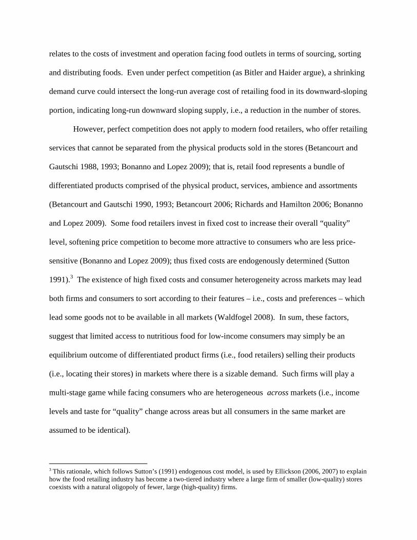
The average marginal effects obtained from the coefficients of the CGOL are reported in

table 3. We remind the reader that the values in the column “LAI=0” represent the average

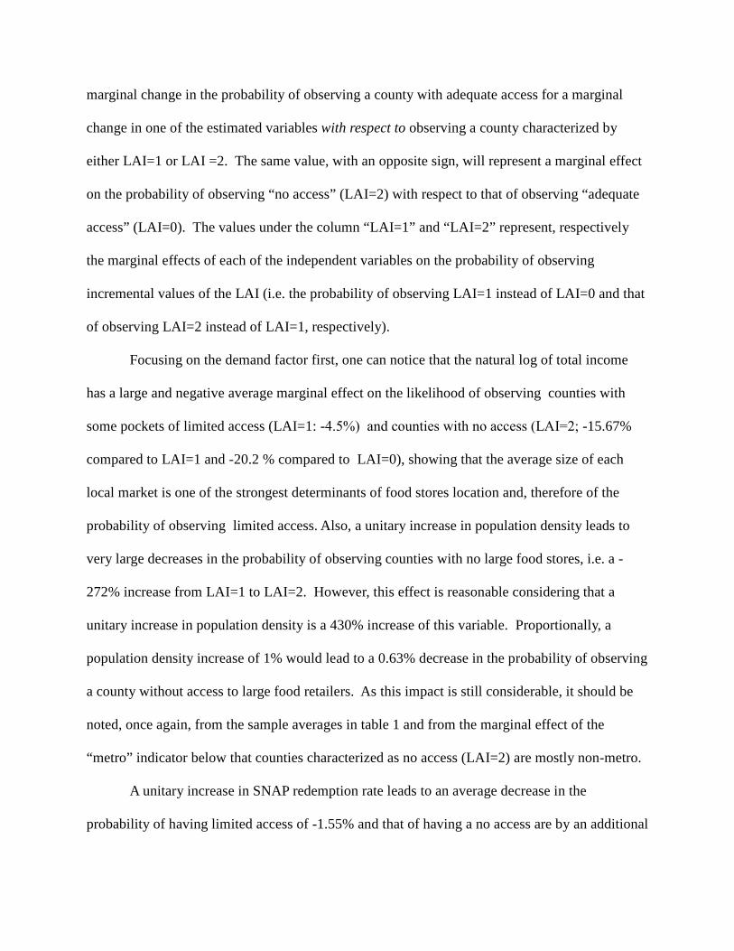
marginal change in the probability of observing a county with adequate access for a marginal

change in one of the estimated variables with respect to observing a county characterized by

either LAI=1 or LAI =2. The same value, with an opposite sign, will represent a marginal effect

on the probability of observing “no access” (LAI=2) with respect to that of observing “adequate

access” (LAI=0). The values under the column “LAI=1” and “LAI=2” represent, respectively

the marginal effects of each of the independent variables on the probability of observing

incremental values of the LAI (i.e. the probability of observing LAI=1 instead of LAI=0 and that

of observing LAI=2 instead of LAI=1, respectively).

Focusing on the demand factor first, one can notice that the natural log of total income

has a large and negative average marginal effect on the likelihood of observing counties with

some pockets of limited access (LAI=1: -4.5%) and counties with no access (LAI=2; -15.67%

compared to LAI=1 and -20.2 % compared to LAI=0), showing that the average size of each

local market is one of the strongest determinants of food stores location and, therefore of the

probability of observing limited access. Also, a unitary increase in population density leads to

very large decreases in the probability of observing counties with no large food stores, i.e. a -

272% increase from LAI=1 to LAI=2. However, this effect is reasonable considering that a

unitary increase in population density is a 430% increase of this variable. Proportionally, a

population density increase of 1% would lead to a 0.63% decrease in the probability of observing

a county without access to large food retailers. As this impact is still considerable, it should be

noted, once again, from the sample averages in table 1 and from the marginal effect of the

“metro” indicator below that counties characterized as no access (LAI=2) are mostly non-metro.

A unitary increase in SNAP redemption rate leads to an average decrease in the

probability of having limited access of -1.55% and that of having a no access are by an additional

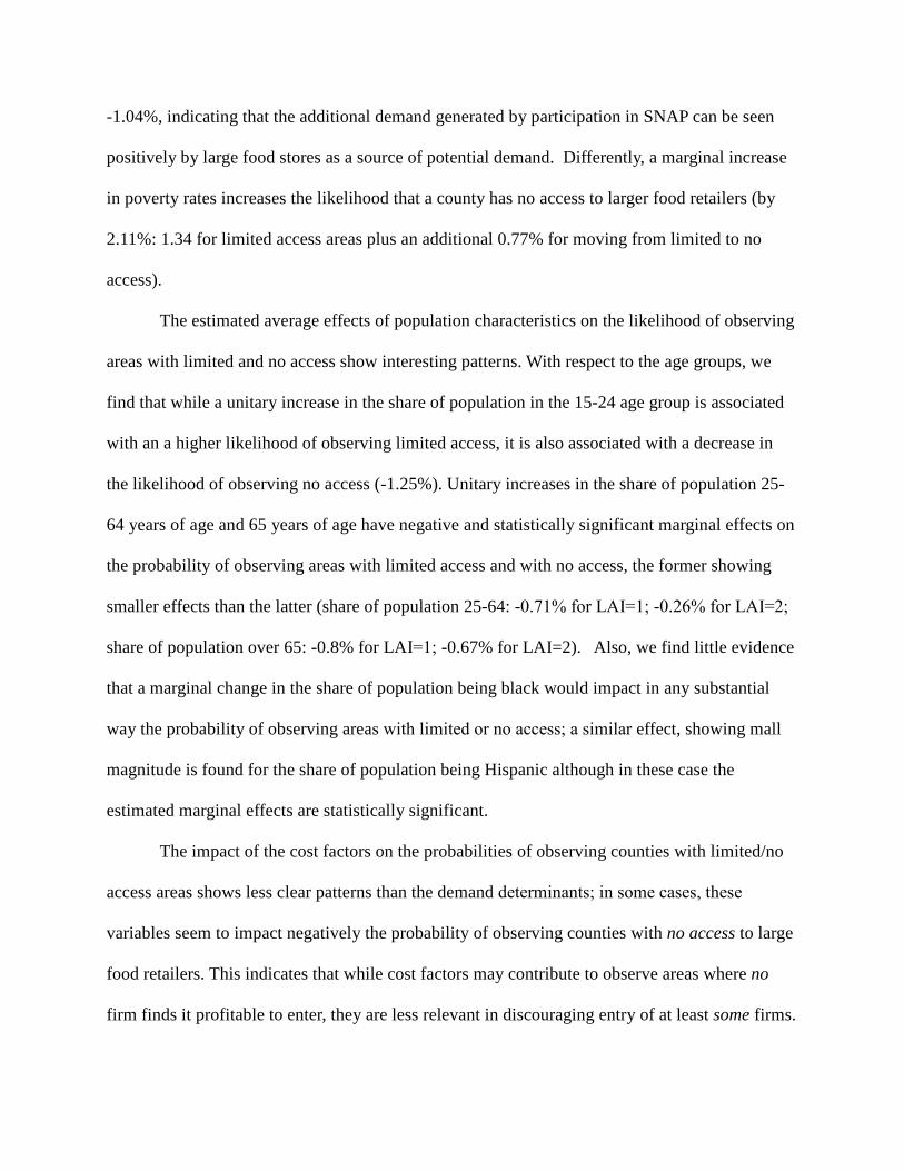
-1.04%, indicating that the additional demand generated by participation in SNAP can be seen

positively by large food stores as a source of potential demand. Differently, a marginal increase

in poverty rates increases the likelihood that a county has no access to larger food retailers (by

2.11%: 1.34 for limited access areas plus an additional 0.77% for moving from limited to no

access).

The estimated average effects of population characteristics on the likelihood of observing

areas with limited and no access show interesting patterns. With respect to the age groups, we

find that while a unitary increase in the share of population in the 15-24 age group is associated

with an a higher likelihood of observing limited access, it is also associated with a decrease in

the likelihood of observing no access (-1.25%). Unitary increases in the share of population 25-

64 years of age and 65 years of age have negative and statistically significant marginal effects on

the probability of observing areas with limited access and with no access, the former showing

smaller effects than the latter (share of population 25-64: -0.71% for LAI=1; -0.26% for LAI=2;

share of population over 65: -0.8% for LAI=1; -0.67% for LAI=2). Also, we find little evidence

that a marginal change in the share of population being black would impact in any substantial

way the probability of observing areas with limited or no access; a similar effect, showing mall

magnitude is found for the share of population being Hispanic although in these case the

estimated marginal effects are statistically significant.

The impact of the cost factors on the probabilities of observing counties with limited/no

access areas shows less clear patterns than the demand determinants; in some cases, these

variables seem to impact negatively the probability of observing counties with no access to large

food retailers. This indicates that while cost factors may contribute to observe areas where no

firm finds it profitable to enter, they are less relevant in discouraging entry of at least some firms.

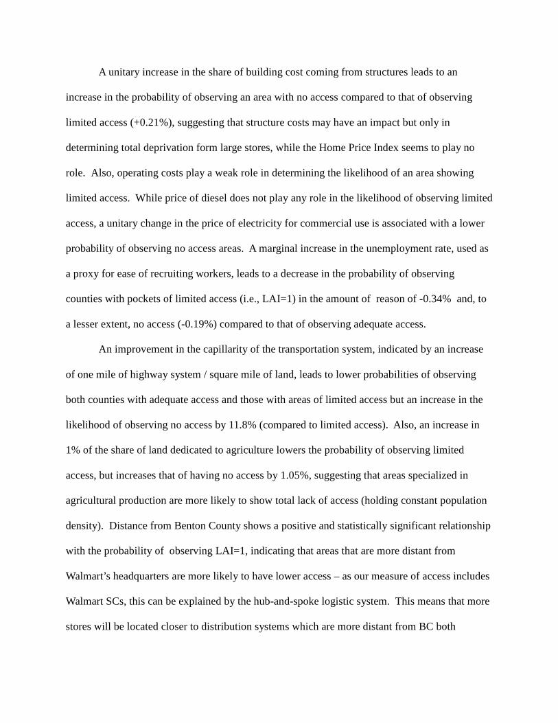
A unitary increase in the share of building cost coming from structures leads to an

increase in the probability of observing an area with no access compared to that of observing

limited access (+0.21%), suggesting that structure costs may have an impact but only in

determining total deprivation form large stores, while the Home Price Index seems to play no

role. Also, operating costs play a weak role in determining the likelihood of an area showing

limited access. While price of diesel does not play any role in the likelihood of observing limited

access, a unitary change in the price of electricity for commercial use is associated with a lower

probability of observing no access areas. A marginal increase in the unemployment rate, used as

a proxy for ease of recruiting workers, leads to a decrease in the probability of observing

counties with pockets of limited access (i.e., LAI=1) in the amount of reason of -0.34% and, to

a lesser extent, no access (-0.19%) compared to that of observing adequate access.

An improvement in the capillarity of the transportation system, indicated by an increase

of one mile of highway system / square mile of land, leads to lower probabilities of observing

both counties with adequate access and those with areas of limited access but an increase in the

likelihood of observing no access by 11.8% (compared to limited access). Also, an increase in

1% of the share of land dedicated to agriculture lowers the probability of observing limited

access, but increases that of having no access by 1.05%, suggesting that areas specialized in

agricultural production are more likely to show total lack of access (holding constant population

density). Distance from Benton County shows a positive and statistically significant relationship

with the probability of observing LAI=1, indicating that areas that are more distant from

Walmart’s headquarters are more likely to have lower access – as our measure of access includes

Walmart SCs, this can be explained by the hub-and-spoke logistic system. This means that more

stores will be located closer to distribution systems which are more distant from BC both

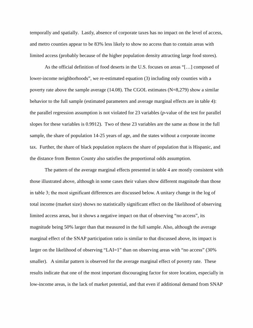
temporally and spatially. Lastly, absence of corporate taxes has no impact on the level of access,

and metro counties appear to be 83% less likely to show no access than to contain areas with

limited access (probably because of the higher population density attracting large food stores).

As the official definition of food deserts in the U.S. focuses on areas “[…] composed of

lower-income neighborhoods”, we re-estimated equation (3) including only counties with a

poverty rate above the sample average (14.08). The CGOL estimates (N=8,279) show a similar

behavior to the full sample (estimated parameters and average marginal effects are in table 4):

the parallel regression assumption is not violated for 23 variables (p-value of the test for parallel

slopes for these variables is 0.9912). Two of these 23 variables are the same as those in the full

sample, the share of population 14-25 years of age, and the states without a corporate income

tax. Further, the share of black population replaces the share of population that is Hispanic, and

the distance from Benton County also satisfies the proportional odds assumption.

The pattern of the average marginal effects presented in table 4 are mostly consistent with

those illustrated above, although in some cases their values show different magnitude than those

in table 3; the most significant differences are discussed below. A unitary change in the log of

total income (market size) shows no statistically significant effect on the likelihood of observing

limited access areas, but it shows a negative impact on that of observing “no access”, its

magnitude being 50% larger than that measured in the full sample. Also, although the average

marginal effect of the SNAP participation ratio is similar to that discussed above, its impact is

larger on the likelihood of observing “LAI=1” than on observing areas with “no access” (30%

smaller). A similar pattern is observed for the average marginal effect of poverty rate. These

results indicate that one of the most important discouraging factor for store location, especially in

low-income areas, is the lack of market potential, and that even if additional demand from SNAP

participants may work as a stimulating factor, it is less relevant in areas where poverty rates are

higher. Both ethnic and age composition of the population show similar or smaller average

effects than those measured in the full sample (with the exclusion of the share of population

between 15-64 years of age).

Also, the average marginal effects of the fixed cost variables are larger than those

obtained using the full sample: in particular, the home price index shows a positive and

significant impact on the likelihood of observing no access; this indicates that cost drivers may

become more important for retailers once they consider the “riskier” decision of locating in areas

with higher poverty rates. Similarly, higher price of diesel seems to result in a higher likelihood

of observing counties characterized by limited access. The other variables show the same

behavior they did in the full sample.

Summary and Conclusions

Using the result provided by Ellickson (2006, 2007) that modeling food retailers as

players of a game where the cost of delivering quality is endogenous (Shaked and Sutton 1987;

Sutton 1991) could lead to areas with limited number of large food stores, we offer an empirical

framework to test the determinants of access to food stores in local markets inside counties. We

assess the probability of local markets to have full, limited and no access to the “high quality”

type of food stores, considering both supply and demand factors to show how limited access can

be an equilibrium outcome of market forces.

We find a clear and consistent path for demand side factors as determining food access

within local markets inside counties, where market size especially (both in terms of total income

and the additional demand from low-income individuals accessing SNAP) explaining a portion

of the location of large food stores. Also, we find that large food stores avoid areas with higher

levels of poverty, and although age composition matters for the likelihood of observing limited

access, ethnic composition matters less; this is important because it suggests that studies showing

a particular ethnic profile in areas characterized by low food access may be observing spuriously

correlated phenomena. However we do find that the share of Hispanic is related to lower levels

of large store access, although the effect is very small; this is probably due to higher demand for

ethnic foods in these communities, which tend to be supplied through smaller outlets. With

respect to the cost factors our results are not as clear, although they show that some cost

determinants, such as the share of the cost of buildings coming from structures, home price index

(more for a sample of counties with high poverty rates), and ease of recruiting labor play a role

in the probability of observing areas with no access. Surprisingly, we find that a favorable tax

regime for businesses has no impact on easing lack of access.

Our analysis confirms that the problem of “food deserts” arises fundamentally due to a

lack of consumer purchasing power and market demand. Simply, if the (fixed) costs of store

operations are not covered by the demand that exists in a particular community, food stores will

cease to operate. As for public policy intervention, it turns out that one federal program is

already playing a key role in attenuating the problem of food access: the SNAP program,

although its role is less marked if one restricts the analysis to counties with poverty rates above

the average. Other potential policy levers (e.g., tax breaks on diesel fuel), and corporate taxes in

particular, appear to play less of a role according to our results. Lowering the cost of capital

investments (perhaps via grants or low-interest loans, though programs similar to the Fresh Food

Financing Initiative in Pennsylvania), could result useful in areas with higher poverty rates,

however, the results are mixed. Somewhat surprisingly, building more roads to enhance access

would have exactly the opposite effect.

Perhaps most paradoxical is the finding with respect to agricultural land shares

(associated with less access even after controlling for other factors). In part this shows the great

disconnect that now exists between food production and consumption. An opportunity may exist

for raising awareness among food system participants of this disconnect, and subsequently re-

localizing or re-regionalizing the food system to assure greater food access. However, whether

such a regionalization would result in a well-functioning food system with greater access, or not,

is an empirical question yet to be answered.

References

Alwitt, L.F., and T.D. Donley. 1997. Retail Stores in Poor Urban Neighbourhoods. The Journal

of Consumer Affairs 31: 139–163.

Asplund, M., and R. Sandin. 1999. The Number of Firms and Production Capacity in Relation to

Market Size. Journal of Industrial Economics 47(1): 69-85.

Ball, K., A. Timperio, and D. Crawford. 2008. Neighborhood Socioeconomic Inequalities in

Food Access and Affordability. Health and Place 15(2): 578–585.

Berry, S.T. 1992. Estimation of a Model of Entry in the Airline Industry. Econometrica 60: 889–

917.

Betancourt, R.R. 2006. The Economics of Retailing and Distribution. Northampton, MA:

Edward Elgar Publishing.

Betancourt, R.R., and D. Gautschi. 1988. The Economics of Retail Firms. Managerial and

Decision Economics 9: 133–44.

Betancourt, R.R., and D. Gautschi. 1990. Demand Complementarities, Household Production,

and Retail Assortments. Marketing Science 9(Spring): 146–61.

Betancourt, R.R., and D. Gautschi. 1993. The Outputs of Retail Activities: Concepts,

Measurement and Evidence from U.S. Census Data. Review of Economics and Statistics

75(2): 294–301.

Bitler, M., and S. J. Haider. 2011. An economic view of food deserts in the United States.

Journal of Policy Analysis and Management 30 (1): 153–176 .

Bonanno, A. 2010. An Empirical Investigation of Wal-Mart’s Expansion into Food Retailing.

Agribusiness: An International Journal 26(2):220–242.

Bonanno, A., and J. Li. 2011. Food Access and Food Security: an Empirical Analysis. Selected

Paper for Presentation at the 2011 AAEA & NAREA Joint Annual Meeting, Pittsburgh,

Pennsylvania, July 24-26, 2011.

Bonanno, A., and R.A. Lopez. 2009. Competition Effects of Supermarket Services. American

Journal of Agricultural Economics 91(3): 555–568.

Bresnahan, T.F., and P.C. Reiss. 1991. Entry and Competition in Concentrated Markets. Journal

of Political Economy 99(5): 977–1009.

Courtemanche, C., and A. Carden. 2011. Supersizing Supercenters? The Impact of Wal-Mart

Supercenters on Body Mass Index and Obesity. Journal of Urban Economics 69(2): 165-

181.

Cummins, S., and S. Macintyre. 2006. Food environments and obesity - Neighborhood or

Nation? International Journal of Epidemiology 35: 100–104.

Cummins, S., Petticrew, M., Higgins, C., Findlay, A., and L. Sparks. 2005. Large Scale Food

Retailing as an Intervention for Diet and Health: Quasi-Experimental Evaluation of a

Natural Experiment. Journal of Epidemiology Community and Health 59: 1035–1040

Drewnowski, A., and N. Darmon. 2005. Food Choices and Diet Costs: an Economic Analysis

The Journal of Nutrition 135: 900-904.

Ellickson, P.B. 2006. Quality Competition in Retailing: A Structural Analysis International

Journal of Industrial Organization 24(3): 521-540.

Ellickson, P.B. 2007. Does Sutton Apply to Supermarkets? RAND Journal of Economics 38(1):

43-59.

Haering, S.A. and S.B. Syed. 2009. Community Food Security in the United States Cities: A

Survey of the Relevant Scientific Literature. Center for a Livable Future, Johns Hopkins

Bloomberg School of Public Health. Available at

http://www.jhsph.edu/bin/s/c/FS_Literature%20Booklet.pdf. Accessed 09/29/2011.

Hawkes, C. 2008. Dietary Implications of Supermarket Development: A Global Perspective.

Development Policy Review 26 (6): 657-692.

Holmes, T.J. 2010. Opening Dates of Wal-Mart Stores and Supercenters, 1962-Jan 31, 2006.

Available at http://www.econ.umn.edu/~holmes/data/WalMart/index.html.

Holmes, T.J. 2011. The Diffusion of Wal-Mart and Economies of Density. Econometrica

79: 253–302.

Holsten, J.E. 2007. Obesity and the community food environment: a systematic review. Public

Health Nutrition 12(3): 397–405.

Jia, P. 2008. What Happens When Wal-Mart Comes to Town: An Empirical Analysis of the

Discount Retail Industry. Econometrica 76(6): 1263-1316.

King, R.P., E.S. Leibtag, and A.S. Behl. 2004. Supermarket Characteristics and Operating Costs

in Low-Income Areas. Agricultural Economic Report N. 839, USDA Economics

Research Service.

Leibtag, E.L., and P.R. Kaufman. 2003. Exploring Food Purchase Behavior of Low-Income

Households How Do They Economize? AIB No. 747-07, USDA Economics Research

Service. Available at www.ers.usda.gov/publications/aib747/aib74707.pdf. Accessed

07/24/2008.

Lincoln Institute of Land Policy. Land and Property Values in the U.S.: Land Prices by State

Database. Available at http://www.lincolninst.edu/subcenters/land-values/land-prices-by-

state.asp. Accessed 07/30/2011.

Long, J.S., and J. Freese. 2006. Regression Models for Categorical Dependent Variables Using

Stata (2nd ed.). College Station, TX: Stata Press.

Moore, L.V., and A. Diez Roux. 2006. Associations of Neighborhood Characteristics with the

Location and Type of Food Stores. Am. Journal of Public Health 96(2): 325–331.

Morris D. A., and J. Heathcote. 2007. The Price and Quantity of Residential Land in the United

States. Journal of Monetary Economics 54(8): 2595-2620.

Morland, K., A. Diez Roux, and S. Wing. 2006. Supermarkets, other food stores, and obesity.

The Atherosclerosis Risk in Communities Study. American Journal of Preventive

Medicine 30: 333-339.

Morton, L. and T. Blanchard. 2007. Starved for access: life in rural America’s food deserts.

Rural Sociological Society.

Powell, L.M., S. Slater, D. Mirtcheva, Y. Bao, and F. J. Chaloupka. 2007. Food Store availability

and Neighborhood Characteristics in the United States. Preventive Medicine 44: 189-195.

Richards, T.J., and S.H. Hamilton. 2006. Rivalry in Price and Variety among Supermarket

Retailers. American Journal of Agricultural Economics 88(3): 710–26.

Rose, D., and R. Richards. 2004. Food Store Access and Household Fruit and Vegetable Use

among Participants in the US Food Stamp Program. Public Health Nutrition 7(8): 1081-

8.

Shaked, A., and J. Sutton. 1987. Product Differentiation and Industrial Structure. Journal of

Industrial Economics 36(2): 131–46.

Sutton, J. 1991. Sunk Cost and Market Structure: Price Competition, Advertising, and the

Evolution of Concentration. Cambridge, MA: MIT Press.

U.S. Bureau of Census. 2001. Gazetteer of counties: Year 2000. Available at

http://www.census.gov/geo/www/gazetteer/places2k.html. Accessed 04/01/2006

U.S. Bureau of Census. Population Estimates Program: 2000- 2006

U.S. Bureau of Labor Statistics. County Business Pattern: 2000-2006.

U.S. Bureau of Labor Statistics. Local Area Unemployment Statistics: 2000-2006.

U.S. Department of Energy. Annual Retail Gasoline and Diesel Prices: Diesel - All Types.

Available at http://www.eia.doe.gov/dnav/pet/pet_pri_gnd_a_epd2d_pte_dpgal_a.htm.

U.S. Department of Energy. Current and Historical Monthly Retail Sales, Revenues and Average

Revenue per KWH by State and by Sector (Form EIA-826) - commercial prices.

U.S. Department of Energy. Energy Information Administration. Refiner Gasoline Prices by

Grade and Sales Type – Regular.

U.S. Department of Transportation. Federal Highway Administration, Highway Statistics:

Section II, Motor Vehicles. State Motor-vehicle Registrations: 2000 – 2006. Available at

http://www.fhwa.dot.gov/policyinformation/statistics.cfm. Accessed 11/10/2011.

U.S. Tax Foundation. Corporate Income Tax Rates: 2000-2011. Available at

http://www.taxfoundation.org/taxdata/show/230.html. Accessed 06/01/2010.

Ver Ploeg, M., V. Breneman, T. Farrigan, K. Hamrick, D. Hopkins, P. Kaufman, B. Lin, M.

Nord, T. Smith, R. Williams, K. Kinnison, C. Olander, A. Sing, and E. Tuckermanty.

2009. Access to Affordable and Nutritious Food—Measuring and Understanding Food

Deserts and Their Consequences: Report to Congress. Publication No. (AP-036), USDA-

ERS, 160 pages. Available at http://www.ers.usda.gov/Publications/AP/AP036/.

Accessed 02/19/2011.

Waldfogel, J. 2008. The Median Voter and the Median Consumer: Local Private Goods and

Residential Sorting. Journal of Urban Economics 63(2): 567-82.

White, M. 2007. Food Access and Obesity. Obesity Reviews (8): 99-107.

Williams, R. 2006. Generalized Ordered Logit/Partial Proportional Odds Models for Ordinal

Dependent Variables. The Stata Journal 6: 58–82.

Zenk, S., A.J. Schulz, B.A. Israel, S.A. James, S. Bao, M.L. Wilson. 2005. Neighborhood Racial

Composition, Neighborhood Poverty, and the Spatial Accessibility of Supermarkets in

Metropolitan Detroit. American Journal of Public Health 95(4): 660–667.

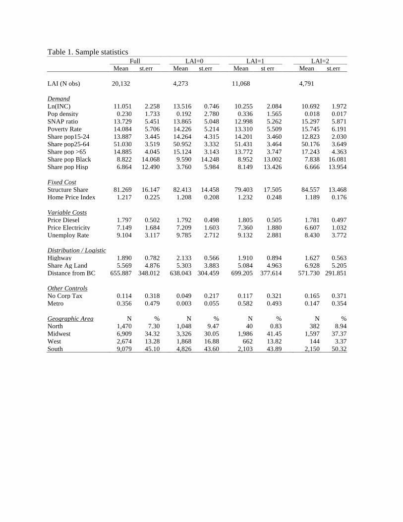
Table 1. Sample statistics Full LAI=0 LAI=1 LAI=2 Mean st.err Mean st.err Mean st err Mean st.err LAI (N obs) 20,132 4,273 11,068 4,791 Demand Ln(INC) 11.051 2.258 13.516 0.746 10.255 2.084 10.692 1.972 Pop density 0.230 1.733 0.192 2.780 0.336 1.565 0.018 0.017 SNAP ratio 13.729 5.451 13.865 5.048 12.998 5.262 15.297 5.871 Poverty Rate 14.084 5.706 14.226 5.214 13.310 5.509 15.745 6.191 Share pop15-24 13.887 3.445 14.264 4.315 14.201 3.460 12.823 2.030 Share pop25-64 51.030 3.519 50.952 3.332 51.431 3.464 50.176 3.649 Share pop >65 14.885 4.045 15.124 3.143 13.772 3.747 17.243 4.363 Share pop Black 8.822 14.068 9.590 14.248 8.952 13.002 7.838 16.081 Share pop Hisp 6.864 12.490 3.760 5.984 8.149 13.426 6.666 13.954 Fixed Cost Structure Share 81.269 16.147 82.413 14.458 79.403 17.505 84.557 13.468 Home Price Index 1.217 0.225 1.208 0.208 1.232 0.248 1.189 0.176 Variable Costs Price Diesel 1.797 0.502 1.792 0.498 1.805 0.505 1.781 0.497 Price Electricity 7.149 1.684 7.209 1.603 7.360 1.880 6.607 1.032 Unemploy Rate 9.104 3.117 9.785 2.712 9.132 2.881 8.430 3.772 Distribution / Logistic Highway 1.890 0.782 2.133 0.566 1.910 0.894 1.627 0.563 Share Ag Land 5.569 4.876 5.303 3.883 5.084 4.963 6.928 5.205 Distance from BC 655.887 348.012 638.043 304.459 699.205 377.614 571.730 291.851 Other Controls No Corp Tax 0.114 0.318 0.049 0.217 0.117 0.321 0.165 0.371 Metro 0.356 0.479 0.003 0.055 0.582 0.493 0.147 0.354 Geographic Area N % N % N % N % North 1,470 7.30 1,048 9.47 40 0.83 382 8.94 Midwest 6,909 34.32 3,326 30.05 1,986 41.45 1,597 37.37 West 2,674 13.28 1,868 16.88 662 13.82 144 3.37 South 9,079 45.10 4,826 43.60 2,103 43.89 2,150 50.32

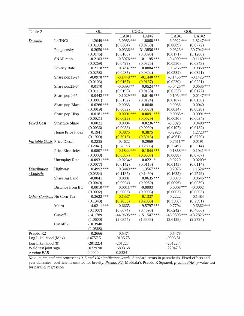
Table 2. OL CGOL GOL LAI=1 LAI=2 LAI=1 LAI=2 Demand Ln(INC) -1.2049 *** -3.0983 *** -1.8068 *** -3.0922 *** -1.8247 *** (0.0199) (0.0684) (0.0760) (0.0689) (0.0772) Pop_density 0.2050 *** 0.0336 ** -31.3856 *** 0.0323 * -30.7042 *** (0.0146) (0.0168) (3.0893) (0.0171) (3.1200) SNAP ratio -0.2103 *** -0.3976 *** -0.1195 *** -0.4009 *** -0.1169 *** (0.0269) (0.0499) (0.0325) (0.0550) (0.0343) Poverty Rate 0.2118 *** 0.3237 *** 0.0884 *** 0.3266 *** 0.0858 *** (0.0258) (0.0485) (0.0304) (0.0534) (0.0321) Share pop15-24 -0.0978 *** -0.1440 *** -0.1440 *** -0.1456 *** -0.1425 *** (0.0103) (0.0167) (0.0167) (0.0230) (0.0221) Share pop25-64 0.0170 -0.0393 ** 0.0524 *** -0.0425 ** 0.0535 *** (0.0111) (0.0196) (0.0158) (0.0253) (0.0177) Share pop >65 0.0442 *** -0.1029 *** 0.0146 *** -0.1054 *** 0.0147 *** (0.0081) (0.0152) (0.0124) (0.0187) (0.0138) Share pop Black 0.0266 *** -0.0033 0.0040 -0.0033 0.0040 (0.0019) (0.0032) (0.0028) (0.0034) (0.0028) Share pop Hisp 0.0181 *** 0.0091 *** 0.0091 *** 0.0085 * 0.0091 *** (0.0021) (0.0029) (0.0029) (0.0050) (0.0034) Fixed Cost Structure Share 0.0031 0.0084 0.0236 *** -0.0028 0.0408 *** (0.0036) (0.0088) (0.0090) (0.0107) (0.0132) Home Price Index 0.1941 0.3875 0.3875 -0.2920 1.2723 ** (0.1900) (0.3915) (0.3915) (0.4961) (0.5729) Variable Costs Price Diesel 0.2235 0.4622 0.2969 0.7511 ** 0.0191 (0.2041) (0.2839) (0.2805) (0.3749) (0.3514) Price Electricity -0.0807 *** -0.1844 *** -0.1844 *** -0.1858 *** -0.1941 *** (0.0303) (0.0507) (0.0507) (0.0688) (0.0707) Unemploy Rate -0.0931 *** -0.0234 * 0.0221 * -0.0220 0.0209 * (0.0077) (0.0142) (0.0113) (0.0145) (0.0114) Distribution Highway 0.4992 *** 0.3449 *** 1.3567 *** 0.2076 1.1524 *** / Logistic (0.0384) (0.1187) (0.1490) (0.1635) (0.2529) Share Ag Land -0.0041 0.0081 0.0635 *** 0.0078 0.0646 *** (0.0040) (0.0094) (0.0059) (0.0096) (0.0059) Distance from BC 0.0010 *** 0.0011 *** -0.0003 0.0008 *** -0.0002 (0.0002) (0.0003) (0.0003) (0.0003) (0.0003) Other Controls No Corp Tax 0.3622 *** 0.1337 0.1337 0.2222 0.1484 (0.1343) (0.2033) (0.2033) (0.3306) (0.2591) Metro -4.0211 *** 0.6665 -9.5797 *** 0.7794 -9.6862 *** (0.1007) (0.6074) (0.4593) (0.6242) (0.4666) Cut-off 1 -14.1789 -44.9695 *** -15.1547 *** -46.9393 *** -13.2825 *** (1.0600) (2.0354) (1.8383) (2.6138) (2.2794) Cut off 2 -10.3940 (1.0568) Pseudo R2 0.2666 0.5474 0.5478 Log Likelihood (Max) -14757.5 -9106.75 -9098.51 Log Likelihood (0) -20122.4 -20122.4 -20122.4 Wald test joint sign 10729.90 5893.68 22047.8 p-value PAR 0.0000 0.8334 Note: *, **, and *** represent 10, 5 and 1% significance levels. Standard errors in parenthesis. Fixed-effects and year dummies’ coefficients omitted for brevity; Pseudo R2: Maddala’s Pseudo R Squared; p-value PAR: p-value test for parallel regression

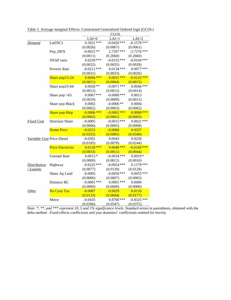
Table 3. Average marginal Effects: Constrained Generalized Ordered logit (GCOL) CGOL LAI=0 LAI=1 LAI=2 Demand Ln(INC) 0.2021 *** -0.0450 *** -0.1570 *** (0.0026) (0.0067) (0.0061) Pop_DEN -0.0022 ** 2.7297 *** -2.7276 *** (0.0011) (0.2660) (0.2660) SNAP ratio 0.0259 *** -0.0155 *** -0.0104 *** (0.0032) (0.0035) (0.0028) Poverty Rate -0.0211 *** 0.0134 *** 0.0077 *** (0.0031) (0.0033) (0.0026) Share pop15-24 0.0094 *** 0.0031 *** -0.0125 *** (0.0011) (0.0004) (0.0015) Share pop25-64 0.0026 ** -0.0071 *** 0.0046 *** (0.0013) (0.0012) (0.0014) Share pop >65 0.0067 *** -0.0080 *** 0.0013 (0.0010) (0.0009) (0.0011) Share pop Black 0.0002 -0.0006 ** 0.0004 (0.0002) (0.0003) (0.0002) Share pop Hisp -0.0006 *** -0.0002 *** 0.0008 *** (0.0002) (0.0001) (0.0003) Fixed Cost Structure Share -0.0005 -0.0015 *** 0.0021 *** (0.0006) (0.0005) (0.0008) Home Price -0.0253 -0.0084 0.0337 (0.0255) (0.0085) (0.0340) Variable Cost Price Diesel -0.0301 0.0043 0.0258 (0.0185) (0.0078) (0.0244) Price Electricity 0.0120 *** 0.0040 *** -0.0160 *** (0.0033) (0.0011) (0.0044) Unempl Rate 0.0015 * -0.0034 *** 0.0019 * (0.0009) (0.0012) (0.0010) Distribution Highway -0.0225 *** -0.0954 *** 0.1179 *** / Logistic (0.0077) (0.0139) (0.0128) Share Ag Land -0.0005 -0.0050 *** 0.0055 *** (0.0006) (0.0007) (0.0005) Distance BC -0.0001 *** 0.0001 *** 0.0000 (0.0000) (0.0000) (0.0000) Other No Corp Tax -0.0087 -0.0029 0.0116 (0.0133) (0.0044) (0.0177) Metro -0.0435 0.8760 *** -0.8325 *** (0.0396) (0.0547) (0.0375) Note: *, **, and *** represent 10, 5 and 1% significance levels. Standard errors in parenthesis, obtained with the delta method . Fixed-effects coefficients and year dummies’ coefficients omitted for brevity

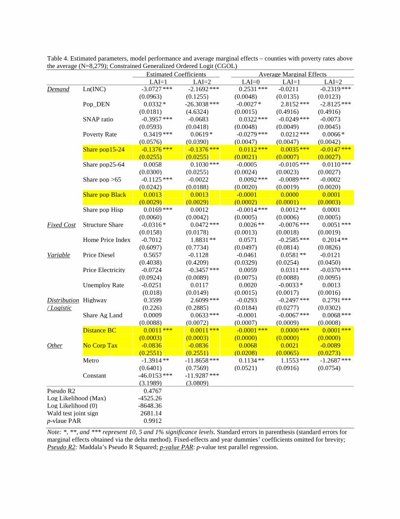
Table 4. Estimated parameters, model performance and average marginal effects – counties with poverty rates above the average (N=8,279); Constrained Generalized Ordered Logit (CGOL) Estimated Coefficients Average Marginal Effects LAI=1 LAI=2 LAI=0 LAI=1 LAI=2 Demand Ln(INC) -3.0727 *** -2.1692 *** 0.2531 *** -0.0211 -0.2319 *** (0.0963) (0.1255) (0.0048) (0.0135) (0.0123) Pop_DEN 0.0332 * -26.3038 *** -0.0027 * 2.8152 *** -2.8125 *** (0.0181) (4.6324) (0.0015) (0.4916) (0.4916) SNAP ratio -0.3957 *** -0.0683 0.0322 *** -0.0249 *** -0.0073 (0.0593) (0.0418) (0.0048) (0.0049) (0.0045) Poverty Rate 0.3419 *** 0.0619 * -0.0279 *** 0.0212 *** 0.0066 * (0.0576) (0.0390) (0.0047) (0.0047) (0.0042) Share pop15-24 -0.1376 *** -0.1376 *** 0.0112 *** 0.0035 *** -0.0147 *** (0.0255) (0.0255) (0.0021) (0.0007) (0.0027) Share pop25-64 0.0058 0.1030 *** -0.0005 -0.0105 *** 0.0110 *** (0.0300) (0.0255) (0.0024) (0.0023) (0.0027) Share pop >65 -0.1125 *** -0.0022 0.0092 *** -0.0089 *** -0.0002 (0.0242) (0.0188) (0.0020) (0.0019) (0.0020) Share pop Black 0.0013 0.0013 -0.0001 0.0000 0.0001 (0.0029) (0.0029) (0.0002) (0.0001) (0.0003) Share pop Hisp 0.0169 *** 0.0012 -0.0014 *** 0.0012 ** 0.0001 (0.0060) (0.0042) (0.0005) (0.0006) (0.0005) Fixed Cost Structure Share -0.0316 * 0.0472 *** 0.0026 ** -0.0076 *** 0.0051 *** (0.0158) (0.0178) (0.0013) (0.0018) (0.0019) Home Price Index -0.7012 1.8831 ** 0.0571 -0.2585 *** 0.2014 ** (0.6097) (0.7734) (0.0497) (0.0814) (0.0826) Variable Price Diesel 0.5657 -0.1128 -0.0461 0.0581 ** -0.0121 (0.4038) (0.4209) (0.0329) (0.0254) (0.0450) Price Electricity -0.0724 -0.3457 *** 0.0059 0.0311 *** -0.0370 *** (0.0924) (0.0089) (0.0075) (0.0088) (0.0095) Unemploy Rate -0.0251 0.0117 0.0020 -0.0033 * 0.0013 (0.018) (0.0149) (0.0015) (0.0017) (0.0016) Distribution Highway 0.3599 2.6099 *** -0.0293 -0.2497 *** 0.2791 *** / Logistic (0.226) (0.2885) (0.0184) (0.0277) (0.0302) Share Ag Land 0.0009 0.0633 *** -0.0001 -0.0067 *** 0.0068 *** (0.0088) (0.0072) (0.0007) (0.0009) (0.0008) Distance BC 0.0011 *** 0.0011 *** -0.0001 *** 0.0000 *** 0.0001 *** (0.0003) (0.0003) (0.0000) (0.0000) (0.0000) Other No Corp Tax -0.0836 -0.0836 0.0068 0.0021 -0.0089 (0.2551) (0.2551) (0.0208) (0.0065) (0.0273) Metro -1.3914 ** -11.8658 *** 0.1134 ** 1.1553 *** -1.2687 *** (0.6401) (0.7569) (0.0521) (0.0916) (0.0754) Constant -46.0153 *** -11.9287 *** (3.1989) (3.0809) Pseudo R2 0.4767 Log Likelihood (Max) -4525.26 Log Likelihood (0) -8648.36 Wald test joint sign 2681.14 p-vlaue PAR 0.9912

Note: *, **, and *** represent 10, 5 and 1% significance levels. Standard errors in parenthesis (standard errors for marginal effects obtained via the delta method). Fixed-effects and year dummies’ coefficients omitted for brevity; Pseudo R2: Maddala’s Pseudo R Squared; p-value PAR: p-value test parallel regression.