
LIMITED DEPENDENT CENSORING, AND SAMPLE...
70
Greene-2140242 book November 27, 2010 18:36 19 LIMITED DEPENDENT VARIABLES—TRUNCATION, CENSORING, AND SAMPLE SELECTION Q 19.1 INTRODUCTION This chapter is concerned with truncation and censoring. As we saw in Section 18.4.6, these features complicate the analysis of data that might otherwise be amenable to conventional estimation methods such as regression. “Truncation” effects arise when one attempts to make inferences about a larger population from a sample that is drawn from a distinct subpopulation. For example, studies of income based on incomes above or below some poverty line may be of limited usefulness for inference about the whole population. Truncation is essentially a characteristic of the distribution from which the sample data are drawn. Censoring is a more common feature of recent studies. To continue the example, suppose that instead of being unobserved, all incomes below the poverty line are reported as if they were at the poverty line. The censoring of a range of values of the variable of interest introduces a distortion into conventional statistical results that is similar to that of truncation. Unlike truncation, however, censoring is essentially a defect in the sample data. Presumably, if they were not censored, the data would be a representative sample from the population of interest. We will also examine a form of truncation called the sample selection problem. Although most empirical work in this area involves censoring rather than truncation, we will study the simpler model of truncation first. It provides most of the theoretical tools we need to analyze models of censoring and sample selection. The discussion will examine the general characteristics of truncation, censoring, and sample selection, and then, in each case, develop a major area of application of the principles. The stochastic frontier model [Aigner, Lovell, and Schmidt (1977), Fried, Lovell, and Schmidt (2008)] is a leading application of results for truncated distributions in empirical models. Censoring appears prominently in the analysis of labor supply and in modeling of duration data. Finally, the sample selection model has appeared in all areas of the social sciences and plays a significant role in the evaluation of treatment effects and program evaluation. 19.2 TRUNCATION In this section, we are concerned with inferring the characteristics of a full population from a sample drawn from a restricted part of that population. 833
Transcript of LIMITED DEPENDENT CENSORING, AND SAMPLE...

Greene-2140242 book November 27, 2010 18:36
19
LIMITED DEPENDENTVARIABLES—TRUNCATION,CENSORING, AND SAMPLE
SELECTION
Q
19.1 INTRODUCTION
This chapter is concerned with truncation and censoring. As we saw in Section 18.4.6,these features complicate the analysis of data that might otherwise be amenable toconventional estimation methods such as regression. “Truncation” effects arise whenone attempts to make inferences about a larger population from a sample that is drawnfrom a distinct subpopulation. For example, studies of income based on incomes aboveor below some poverty line may be of limited usefulness for inference about the wholepopulation. Truncation is essentially a characteristic of the distribution from whichthe sample data are drawn. Censoring is a more common feature of recent studies. Tocontinue the example, suppose that instead of being unobserved, all incomes below thepoverty line are reported as if they were at the poverty line. The censoring of a rangeof values of the variable of interest introduces a distortion into conventional statisticalresults that is similar to that of truncation. Unlike truncation, however, censoring isessentially a defect in the sample data. Presumably, if they were not censored, the datawould be a representative sample from the population of interest. We will also examinea form of truncation called the sample selection problem. Although most empiricalwork in this area involves censoring rather than truncation, we will study the simplermodel of truncation first. It provides most of the theoretical tools we need to analyzemodels of censoring and sample selection.
The discussion will examine the general characteristics of truncation, censoring,and sample selection, and then, in each case, develop a major area of application of theprinciples. The stochastic frontier model [Aigner, Lovell, and Schmidt (1977), Fried,Lovell, and Schmidt (2008)] is a leading application of results for truncated distributionsin empirical models. Censoring appears prominently in the analysis of labor supply andin modeling of duration data. Finally, the sample selection model has appeared in allareas of the social sciences and plays a significant role in the evaluation of treatmenteffects and program evaluation.
19.2 TRUNCATION
In this section, we are concerned with inferring the characteristics of a full populationfrom a sample drawn from a restricted part of that population.
833

Greene-2140242 book November 27, 2010 18:36
834 PART IV ✦ Cross Sections, Panel Data, and Microeconometrics
19.2.1 TRUNCATED DISTRIBUTIONS
A truncated distribution is the part of an untruncated distribution that is above or belowsome specified value. For instance, in Example 19.2, we are given a characteristic of thedistribution of incomes above $100,000. This subset is a part of the full distribution ofincomes which range from zero to (essentially) infinity.
THEOREM 19.1 Density of a Truncated Random VariableIf a continuous random variable x has pdf f (x) and a is a constant, then1
f (x | x > a) = f (x)
Prob(x > a).
The proof follows from the definition of conditional probability and amountsmerely to scaling the density so that it integrates to one over the range above a.Note that the truncated distribution is a conditional distribution.
Most recent applications based on continuous random variables use the truncatednormal distribution. If x has a normal distribution with mean μ and standard deviationσ, then
Prob(x > a) = 1 − �
(a − μ
σ
)= 1 − �(α),
where α = (a − μ)/σ and �(.) is the standard normal cdf. The density of the truncatednormal distribution is then
f (x | x > a) = f (x)
1 − �(α)= (2πσ 2)−1/2e−(x−μ)2/(2σ 2)
1 − �(α)=
1σ
φ
(x − μ
σ
)1 − �(α)
,
where φ(.) is the standard normal pdf. The truncated standard normal distribution, withμ = 0 and σ = 1, is illustrated for a = −0.5, 0, and 0.5 in Figure 19.1. Another truncateddistribution that has appeared in the recent literature, this one for a discrete randomvariable, is the truncated at zero Poisson distribution,
Prob[Y = y | y > 0] = (e−λλy)/y!Prob[Y > 0]
= (e−λλy)/y!1 − Prob[Y = 0]
= (e−λλy)/y!1 − e−λ
, λ > 0, y = 1, . . .
This distribution is used in models of uses of recreation and other kinds of facilitieswhere observations of zero uses are discarded.2
For convenience in what follows, we shall call a random variable whose distributionis truncated a truncated random variable.
1The case of truncation from above instead of below is handled in an analogous fashion and does not requireany new results.2See Shaw (1988). An application of this model appears in Section 18.4.6 and Example 18.8.

Greene-2140242 book November 27, 2010 18:36
CHAPTER 19 ✦ Limited Dependent Variables 835
�3 �2 �1 �0.5 0
Den
sity
0
0.2
0.4
0.6
0.8
1.0
1.2
x0.5 1 2 3
Truncation pointMean of distribution
FIGURE 19.1 Truncated Normal Distributions.
19.2.2 MOMENTS OF TRUNCATED DISTRIBUTIONS
We are usually interested in the mean and variance of the truncated random variable.They would be obtained by the general formula:
E [x | x > a] =∫ ∞
ax f (x | x > a) dx
for the mean and likewise for the variance.
Example 19.1 Truncated Uniform DistributionIf x has a standard uniform distribution, denoted U (0, 1) , then
f ( x) = 1, 0 ≤ x ≤ 1.
The truncated at x = 13 distribution is also uniform:
f
(x | x >
13
)= f ( x)
Prob(x > 1
3
) = 1(23
) = 32
,13
≤ x ≤ 1.
The expected value is
E
[x | x >
13
]=
∫ 1
1/3
x
(32
)dx = 2
3.
For a variable distributed uniformly between L and U , the variance is (U − L ) 2/12.Thus,
Var[x | x >
13
]= 1
27.
The mean and variance of the untruncated distribution are 12 and 1
12 , respectively.

Greene-2140242 book November 27, 2010 18:36
836 PART IV ✦ Cross Sections, Panel Data, and Microeconometrics
Example 19.1 illustrates two results.
1. If the truncation is from below, then the mean of the truncated variable is greaterthan the mean of the original one. If the truncation is from above, then the meanof the truncated variable is smaller than the mean of the original one.
2. Truncation reduces the variance compared with the variance in the untruncateddistribution.
Henceforth, we shall use the terms truncated mean and truncated variance to refer tothe mean and variance of the random variable with a truncated distribution.
For the truncated normal distribution, we have the following theorem:3
THEOREM 19.2 Moments of the Truncated Normal DistributionIf x ∼ N[μ, σ 2] and a is a constant, then
E [x | truncation] = μ + σλ(α), (19-1)
Var[x | truncation] = σ 2[1 − δ(α)], (19-2)
where α = (a − μ)/σ, φ(α) is the standard normal density and
λ(α) = φ(α)/[1 − �(α)] if truncation is x > a, (19-3a)
λ(α) = −φ(α)/�(α) if truncation is x < a, (19-3b)
and
δ(α) = λ(α)[λ(α) − α]. (19-4)
An important result is
0 < δ(α) < 1 for all values of α,
which implies point 2 after Example 19.1. A result that we will use at several points belowis dφ(α)/dα = −αφ(α). The function λ(α) is called the inverse Mills ratio. The functionin (19-3a) is also called the hazard function for the standard normal distribution.
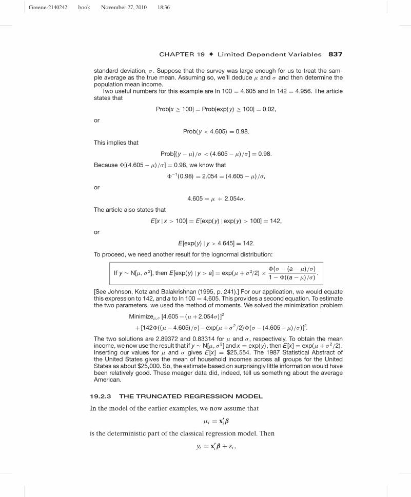
Example 19.2 A Truncated Lognormal Income Distribution“The typical ‘upper affluent American’ . . . makes $142,000 per year . . . . The people surveyedhad household income of at least $100,000.”4 Would this statistic tell us anything about the“typical American”? As it stands, it probably does not (popular impressions notwithstanding).The 1987 article where this appeared went on to state, “If you’re in that category, pat yourselfon the back—only 2 percent of American households make the grade, according to thesurvey.” Because the degree of truncation in the sample is 98 percent, the $142,000 wasprobably quite far from the mean in the full population.
Suppose that incomes, x, in the population were lognormally distributed—see Sec-tion B.4.4. Then the log of income, y, had a normal distribution with, say, mean μ and
3Details may be found in Johnson, Kotz, and Balakrishnan (1994, pp. 156–158). Proofs appear in Cameronand Trivedi (2005).4See New York Post (1987).
Greene-2140242 book November 27, 2010 18:36
CHAPTER 19 ✦ Limited Dependent Variables 837
standard deviation, σ . Suppose that the survey was large enough for us to treat the sam-ple average as the true mean. Assuming so, we’ll deduce μ and σ and then determine thepopulation mean income.
Two useful numbers for this example are In 100 = 4.605 and In 142 = 4.956. The articlestates that
Prob[x ≥ 100] = Prob[exp( y) ≥ 100] = 0.02,
or
Prob( y < 4.605) = 0.98.
This implies that
Prob[( y − μ)/σ < (4.605 − μ)/σ ] = 0.98.
Because �[(4.605 − μ)/σ ] = 0.98, we know that
�−1(0.98) = 2.054 = (4.605 − μ)/σ,
or
4.605 = μ + 2.054σ.
The article also states that
E [x | x > 100] = E [exp( y) | exp( y) > 100] = 142,
or
E [exp( y) | y > 4.645] = 142.
To proceed, we need another result for the lognormal distribution:
If y ∼ N[μ, σ 2], then E [exp( y) | y > a] = exp(μ + σ 2/2) × �(σ − (a − μ)/σ )1 − �( (a − μ)/σ )
.
[See Johnson, Kotz and Balakrishnan (1995, p. 241).] For our application, we would equatethis expression to 142, and a to In 100 = 4.605. This provides a second equation. To estimatethe two parameters, we used the method of moments. We solved the minimization problem
Minimizeμ,σ [4.605 − (μ + 2.054σ ) ]2
+ [142�( (μ − 4.605)/σ )− exp(μ + σ 2/2)�(σ − (4.605 − μ)/σ ) ]2.
The two solutions are 2.89372 and 0.83314 for μ and σ , respectively. To obtain the meanincome, we now use the result that if y ∼ N[μ, σ 2] and x = exp( y) , then E [x] = exp(μ + σ 2/2) .Inserting our values for μ and σ gives E [x] = $25,554. The 1987 Statistical Abstract ofthe United States gives the mean of household incomes across all groups for the UnitedStates as about $25,000. So, the estimate based on surprisingly little information would havebeen relatively good. These meager data did, indeed, tell us something about the averageAmerican.
19.2.3 THE TRUNCATED REGRESSION MODEL
In the model of the earlier examples, we now assume that
μi = x′iβ
is the deterministic part of the classical regression model. Then
yi = x′iβ + εi ,
Greene-2140242 book November 27, 2010 18:36
838 PART IV ✦ Cross Sections, Panel Data, and Microeconometrics
where
εi | xi ∼ N[0, σ 2],
so that
yi | xi ∼ N[x′iβ, σ 2]. (19-5)
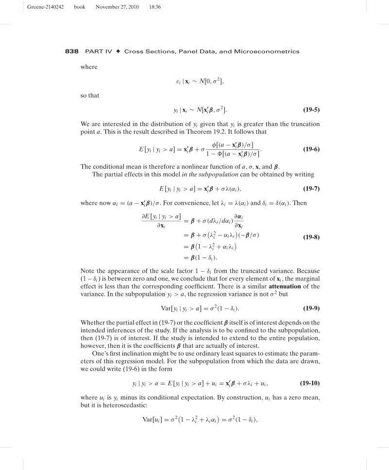
We are interested in the distribution of yi given that yi is greater than the truncationpoint a. This is the result described in Theorem 19.2. It follows that
E [yi | yi > a] = x′iβ + σ
φ[(a − x′iβ)/σ ]
1 − �[(a − x′iβ)/σ ]
. (19-6)
The conditional mean is therefore a nonlinear function of a, σ, x, and β.The partial effects in this model in the subpopulation can be obtained by writing
E [yi | yi > a] = x′iβ + σλ(αi ), (19-7)
where now αi = (a − x′iβ)/σ . For convenience, let λi = λ(αi ) and δi = δ(αi ). Then
∂E [yi | yi > a]∂xi
= β + σ(dλi/dαi )∂αi
∂xi
= β + σ(λ2
i − αiλi)(−β/σ)
= β(1 − λ2
i + αiλi)
= β(1 − δi ).
(19-8)
Note the appearance of the scale factor 1 − δi from the truncated variance. Because(1 − δi ) is between zero and one, we conclude that for every element of xi , the marginaleffect is less than the corresponding coefficient. There is a similar attenuation of thevariance. In the subpopulation yi > a, the regression variance is not σ 2 but
Var[yi | yi > a] = σ 2(1 − δi ). (19-9)
Whether the partial effect in (19-7) or the coefficient β itself is of interest depends on theintended inferences of the study. If the analysis is to be confined to the subpopulation,then (19-7) is of interest. If the study is intended to extend to the entire population,however, then it is the coefficients β that are actually of interest.
One’s first inclination might be to use ordinary least squares to estimate the param-eters of this regression model. For the subpopulation from which the data are drawn,we could write (19-6) in the form
yi | yi > a = E [yi | yi > a] + ui = x′iβ + σλi + ui , (19-10)
where ui is yi minus its conditional expectation. By construction, ui has a zero mean,but it is heteroscedastic:
Var[ui ] = σ 2(1 − λ2i + λiαi
) = σ 2(1 − δi ),
Greene-2140242 book November 27, 2010 18:36
CHAPTER 19 ✦ Limited Dependent Variables 839
which is a function of xi . If we estimate (19-10) by ordinary least squares regression ofy on X, then we have omitted a variable, the nonlinear term λi . All the biases that arisebecause of an omitted variable can be expected.5
Without some knowledge of the distribution of x, it is not possible to determinehow serious the bias is likely to be. A result obtained by Chung and Goldberger(1984) is broadly suggestive. If E [x | y] in the full population is a linear function ofy, then plim b = βτ for some proportionality constant τ . This result is consistent withthe widely observed (albeit rather rough) proportionality relationship between leastsquares estimates of this model and maximum likelihood estimates.6 The proportional-ity result appears to be quite general. In applications, it is usually found that, comparedwith consistent maximum likelihood estimates, the OLS estimates are biased towardzero. (See Example 19.5.)
19.2.4 THE STOCHASTIC FRONTIER MODEL
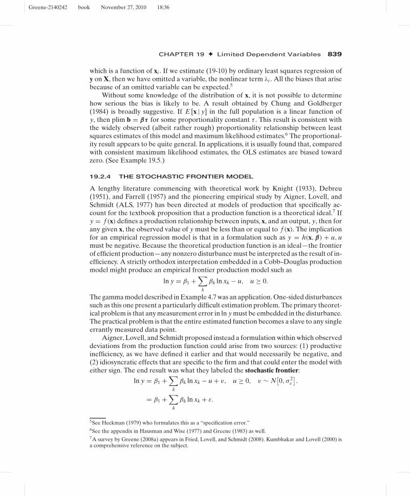
A lengthy literature commencing with theoretical work by Knight (1933), Debreu(1951), and Farrell (1957) and the pioneering empirical study by Aigner, Lovell, andSchmidt (ALS, 1977) has been directed at models of production that specifically ac-count for the textbook proposition that a production function is a theoretical ideal.7 Ify = f (x) defines a production relationship between inputs, x, and an output, y, then forany given x, the observed value of y must be less than or equal to f (x). The implicationfor an empirical regression model is that in a formulation such as y = h(x, β) + u, umust be negative. Because the theoretical production function is an ideal—the frontierof efficient production—any nonzero disturbance must be interpreted as the result of in-efficiency. A strictly orthodox interpretation embedded in a Cobb–Douglas productionmodel might produce an empirical frontier production model such as
ln y = β1 +∑
k
βk ln xk − u, u ≥ 0.
The gamma model described in Example 4.7 was an application. One-sided disturbancessuch as this one present a particularly difficult estimation problem. The primary theoret-ical problem is that any measurement error in ln y must be embedded in the disturbance.The practical problem is that the entire estimated function becomes a slave to any singleerrantly measured data point.
Aigner, Lovell, and Schmidt proposed instead a formulation within which observeddeviations from the production function could arise from two sources: (1) productiveinefficiency, as we have defined it earlier and that would necessarily be negative, and(2) idiosyncratic effects that are specific to the firm and that could enter the model witheither sign. The end result was what they labeled the stochastic frontier:
ln y = β1 +∑
k
βk ln xk − u + v, u ≥ 0, v ∼ N[0, σ 2
v
].
= β1 +∑
k
βk ln xk + ε.
5See Heckman (1979) who formulates this as a “specification error.”6See the appendix in Hausman and Wise (1977) and Greene (1983) as well.7A survey by Greene (2008a) appears in Fried, Lovell, and Schmidt (2008). Kumbhakar and Lovell (2000) isa comprehensive reference on the subject.

Greene-2140242 book November 27, 2010 18:36
840 PART IV ✦ Cross Sections, Panel Data, and Microeconometrics
The frontier for any particular firm is h(x, β)+v, hence the name stochastic frontier. Theinefficiency term is u, a random variable of particular interest in this setting. Becausethe data are in log terms, u is a measure of the percentage by which the particularobservation fails to achieve the frontier, ideal production rate.
To complete the specification, they suggested two possible distributions for the in-efficiency term: the absolute value of a normally distributed variable, which has thetruncated at zero distribution shown in Figure 19.1, and an exponentially distributedvariable. The density functions for these two compound variables are given by Aigner,Lovell, and Schmidt; let ε = v − u, λ = σu/σv, σ = (σ 2
u + σ 2v )1/2, and �(z) = the prob-
ability to the left of z in the standard normal distribution (see Section B.4.1). For the“half-normal” model,
ln h(εi | β, λ, σ ) =[−ln σ +
(12
)ln
2π
− 12
(εi
σ
)2
+ ln �
(−εiλ
σ
)],
whereas for the exponential model
ln h(εi | β, θ, σv) =[
ln θ + 12θ2σ 2
v + θεi + ln �
(− εi
σv
− θσv
)].
Both these distributions are asymmetric. We thus have a regression model with anonnormal distribution specified for the disturbance. The disturbance, ε, has a nonzeromean as well; E [ε] = −σu(2/π)1/2 for the half-normal model and −1/θ for the expo-nential model. Figure 19.2 illustrates the density for the half-normal model with σ = 1and λ = 2. By writing β0 = β1 + E [ε] and ε∗ = ε− E [ε], we obtain a more conventionalformulation
ln y = β0 +∑
k
βk ln xk + ε∗,
FIGURE 19.2 Density for the Disturbance in the Stochastic FrontierModel.
�2.8 �1.6
Den
sity
�0.4�
0.8 2.0�4.00.00
0.70
0.56
0.42
0.28
0.14
Greene-2140242 book November 27, 2010 18:36
CHAPTER 19 ✦ Limited Dependent Variables 841
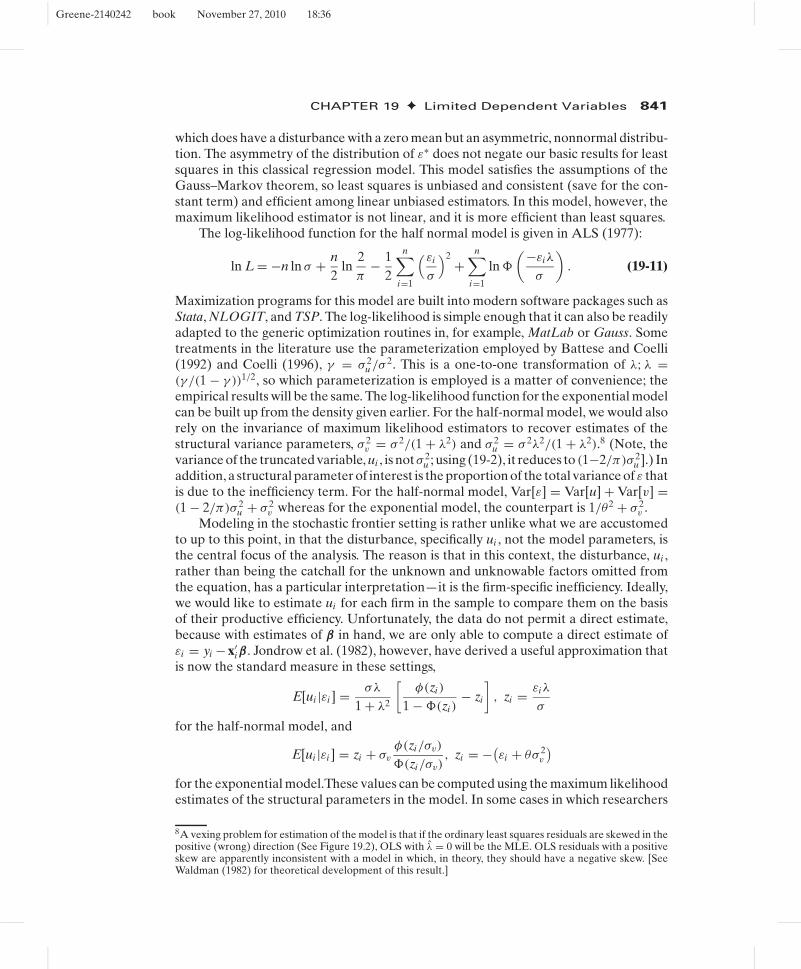
which does have a disturbance with a zero mean but an asymmetric, nonnormal distribu-tion. The asymmetry of the distribution of ε∗ does not negate our basic results for leastsquares in this classical regression model. This model satisfies the assumptions of theGauss–Markov theorem, so least squares is unbiased and consistent (save for the con-stant term) and efficient among linear unbiased estimators. In this model, however, themaximum likelihood estimator is not linear, and it is more efficient than least squares.
The log-likelihood function for the half normal model is given in ALS (1977):
ln L = −n ln σ + n2
ln2π
− 12
n∑i=1
(εi
σ
)2+
n∑i=1
ln �
(−εiλ
σ
). (19-11)
Maximization programs for this model are built into modern software packages such asStata, NLOGIT, and TSP. The log-likelihood is simple enough that it can also be readilyadapted to the generic optimization routines in, for example, MatLab or Gauss. Sometreatments in the literature use the parameterization employed by Battese and Coelli(1992) and Coelli (1996), γ = σ 2
u /σ 2. This is a one-to-one transformation of λ; λ =(γ /(1 − γ ))1/2, so which parameterization is employed is a matter of convenience; theempirical results will be the same. The log-likelihood function for the exponential modelcan be built up from the density given earlier. For the half-normal model, we would alsorely on the invariance of maximum likelihood estimators to recover estimates of thestructural variance parameters, σ 2
v = σ 2/(1 + λ2) and σ 2u = σ 2λ2/(1 + λ2).8 (Note, the
variance of the truncated variable, ui , is notσ 2u ; using (19-2), it reduces to (1−2/π)σ 2
u ].) Inaddition, a structural parameter of interest is the proportion of the total variance of ε thatis due to the inefficiency term. For the half-normal model, Var[ε] = Var[u] + Var[v] =(1 − 2/π)σ 2
u + σ 2v whereas for the exponential model, the counterpart is 1/θ2 + σ 2
v .Modeling in the stochastic frontier setting is rather unlike what we are accustomed
to up to this point, in that the disturbance, specifically ui , not the model parameters, isthe central focus of the analysis. The reason is that in this context, the disturbance, ui ,rather than being the catchall for the unknown and unknowable factors omitted fromthe equation, has a particular interpretation—it is the firm-specific inefficiency. Ideally,we would like to estimate ui for each firm in the sample to compare them on the basisof their productive efficiency. Unfortunately, the data do not permit a direct estimate,because with estimates of β in hand, we are only able to compute a direct estimate ofεi = yi − x′
iβ. Jondrow et al. (1982), however, have derived a useful approximation thatis now the standard measure in these settings,
E[ui |εi ] = σλ
1 + λ2
[φ(zi )
1 − �(zi )− zi
], zi = εiλ
σ
for the half-normal model, and
E[ui |εi ] = zi + σv
φ(zi/σv)
�(zi/σv), zi = −(
εi + θσ 2v
)for the exponential model.These values can be computed using the maximum likelihoodestimates of the structural parameters in the model. In some cases in which researchers
8A vexing problem for estimation of the model is that if the ordinary least squares residuals are skewed in thepositive (wrong) direction (See Figure 19.2), OLS with λ = 0 will be the MLE. OLS residuals with a positiveskew are apparently inconsistent with a model in which, in theory, they should have a negative skew. [SeeWaldman (1982) for theoretical development of this result.]

Greene-2140242 book November 27, 2010 18:36
842 PART IV ✦ Cross Sections, Panel Data, and Microeconometrics
are interested in discovering best practice [e.g., WHO (2000), Tandon et al. (2000)], theestimated values are sorted and the ranks of the individuals in the sample become ofinterest.
Research in this area since the methodological developments beginning in the 1930sand the building of the empirical foundations in 1977 and 1982 has proceeded in severaldirections. Most theoretical treatments of “inefficiency” as envisioned here attribute it toaspects of management of the firm. It remains to establish a firm theoretical connectionbetween the theory of firm behavior and the stochastic frontier model as a device formeasurement of inefficiency.
In the context of the model, many studies have developed alternative, more flexiblefunctional forms that (it is hoped) can provide a more realistic model for inefficiency.Two that are relevant in this chapter are Stevenson’s (1980) truncated normal modeland the normal-gamma frontier. One intuitively appealing form of the truncated normalmodel is
Ui ∼ N[μ + z′
iα, σ 2u
],
ui = |Ui |.The original normal–half-normal model results if μ equals zero and α equals zero. Thisis a device by which the environmental variables noted in the next paragraph can enterthe model of inefficiency. A truncated normal model is presented in Example 19.3. Thehalf-normal, truncated normal, and exponential models all take the form of distributionshown in Figure 19.1. The gamma model,
f (u) = [θ P/�(P)] exp(−θu)uP−1,
is a flexible model that presents the advantage that the distribution of inefficiency canmove away from zero. If P is greater than one, then the density at u = 0 equals zeroand the entire distribution moves away from the origin. The implication is that thedistribution of inefficiency among firms can move away from zero. The gamma model isestimated by simulation methods—either Bayesian MCMC [Huang (2003) and Tsionas(2002)] or maximum simulated likelihood [Greene (2003)]. Many other functional formshave been proposed. [See Greene (2008) for a survey.]
There are usually elements in the environment in which the firm operates thatimpact the firm’s output and/or costs but are not, themselves, outputs, inputs, or inputprices. In example 19.3, the costs of the Swiss railroads are affected by three variables;track width, long tunnels, and curvature. It is not yet specified how such factors should beincorporated into the model; four candidates are in the mean and variance of ui , directlyin the function, or in the variance of vi . [See Hadri, Guermat, and Whittaker (2003) andKumbhakar (1997c).] All of these can be found in the received studies. This aspect ofthe model was prominent in the discussion of the famous World Health Organizationefficiency study of world health systems [WHO (2000), Tandon, Murray, Lauer, andEvans (2000), and Greene (2004)]. In Example 19.3, we have placed the environmentalfactors in the mean of the inefficiency distribution. This produces a rather extremeset of results for the JLMS estimates of inefficiency—many railroads are estimatedto be extremely inefficient. An alternative formulation would be a “heteroscedastic”model in which σu,i = σu exp(z′
iδ) or σv,i = σv exp(z′iη), or both. We can see from the
JLMS formula that the term heteroscedastic is actually a bit misleading, since both

Greene-2140242 book November 27, 2010 18:36
CHAPTER 19 ✦ Limited Dependent Variables 843
standard deviations enter (now) λi , which is, in turn, a crucial parameter in the meanof inefficiency.
How should inefficiency be modeled in panel data, such as in our example? Itmight be tempting to treat it as a time-invariant “effect” [as in Schmidt and Sickles(1984) and Pitt and Lee (1984) in two pioneering papers]. Greene (2004) argued that apreferable approach would be to allow inefficiency to vary freely over time in a panel,and to the extent that there is a common time-invariant effect in the model, that shouldbe treated as unobserved heterogeneity, not inefficiency. A string of studies, includingBattese and Coelli (1992, 1995), Cuesta (2000), Kumbhakar (1997a) Kumbhakar andOrea (2004), and many others have proposed hybrid forms that treat the core randompart of inefficiency as a time-invariant firm-specific effect that is modified over time bya deterministic, possibly firm-specific, function. The Battese-Coelli form,
uit = exp[−η(t − T)]|Ui | where Ui N[0, σ 2
u
],
has been used in a number of applications. Cuesta (2000) suggests allowing η to varyacross firms, producing a model that bears some relationship to a fixed-effects specifi-cation. This thread of the literature is one of the most active ongoing pursuits.
Is it reasonable to use a possibly restrictive parametric approach to modeling in-efficiency? Sickles (2005) and Kumbhakar, Simar, Park, and Tsionas (2007) are amongnumerous studies that have explored less parametric approaches to efficiency analysis.Proponents of data envelopment analysis [see, e.g., Simar and Wilson (2000, 2007)] havedeveloped methods that impose absolutely no parametric structure on the productionfunction. Among the costs of this high degree of flexibility is a difficulty to include envi-ronmental effects anywhere in the analysis, and the uncomfortable implication that anyunmeasured heterogeneity of any sort is necessarily included in the measure of ineffi-ciency. That is, data envelopment analysis returns to the deterministic frontier approachwhere this section began.
Example 19.3 Stochastic Cost Frontier for Swiss RailroadsFarsi, Filippini, and Greene (2005) analyzed the cost efficiency of Swiss railroads. In order touse the stochastic frontier approach to analyze costs of production, rather than production,we rely on the fundamental duality of production and cost [see Samuelson (1938), Shephard(1953), and Kumbhakar and Lovell (2000)]. An appropriate cost frontier model for a firm thatproduces more than one output—the Swiss railroads carry both freight and passengers—willappear as the following:
ln(C/PK ) = α +K−1∑k=1
βk ln( Pk/PK ) +M∑
m=1
γm ln Qm + v + u.
The requirement that the cost function be homogeneous of degree one in the input priceshas been imposed by normalizing total cost, C, and the first K − 1 prices by the K th inputprice. In this application, the three factors are labor, capital, and electricity—the third isused as the numeraire in the cost function. Notice that the inefficiency term, u, enters thecost function positively; actual cost is above the frontier cost. [The MLE is modified simply byreplacing εi with −εi in (19-11).] In analyzing costs of production, we recognize that there is anadditional source of inefficiency that is absent when we analyze production. On the productionside, inefficiency measures the difference between output and frontier output, which arisesbecause of technical inefficiency. By construction, if output fails to reach the efficient levelfor the given input usage, then costs must be higher than frontier costs. However, costs canbe excessive even if the firm is technically efficient if it is “allocatively inefficient.” That is, thefirm can be technically efficient while not using inputs in the cost minimizing mix (equating

Greene-2140242 book November 27, 2010 18:36
844 PART IV ✦ Cross Sections, Panel Data, and Microeconometrics
the ratio of marginal products to the input price ratios). It follows that on the cost side, “u”can contain both elements of inefficiency while on the production side, we would expect tomeasure only technical inefficiency. [See Kumbhakar (1997b).]
The data for this study are an unbalanced panel of 50 railroads with Ti ranging from 1to 13. (Thirty-seven of the firms are observed 13 times, 8 are observed 12 times, and theremaining 5 are observed 10, 7, 7, 3, and 1 times.) The variables we will use here are
CT: Total costs adjusted for inflation (1,000 Swiss franc)QP: Total passenger-output in passenger-kilometersQF: Total goods-output in ton-kilometersPL: Labor price adjusted for inflation (in Swiss Francs per person per year)PK: Capital price with capital stock proxied by total number of seatsPE: Price of electricity (Swiss franc per kWh)
Logs of costs and prices (ln CT, ln PK, ln PL) are normalized by PE. We will also use theseenvironmental variables:
NARROW T: Dummy for the networks with narrow track (1 m wide) The usualwidth is 1.435m.
TUNNEL: Dummy for networks that have tunnels with an average lengthof more than 300 meters.
VIRAGE: Dummy for the networks whose minimum radius of curvature is100 meters or less.
The full data set is given in Appendix Table F19.1. Several other variables not used here arepresented in the appendix table. In what follows, we will ignore the panel data aspect of thedata set. This would be a focal point of a more extensive study.
There have been dozens of models proposed for the inefficiency component of thestochastic frontier model. Table 19.1 presents several different forms. The basic half-normalmodel is given in the first column. The estimated cost function parameters across the different
TABLE 19.1 Estimated Stochastic Frontier Cost Functionsa
Model
Half TruncatedVariable Normal Normal Exponential Gamma Heterosced Heterogen
Constant −10.0799 −9.80624 −10.1838 −10.1944 −9.82189 −10.2891ln QP 0.64220 0.62573 0.64403 0.64401 0.61976 0.63576ln QF 0.06904 0.07708 0.06803 0.06810 0.07970 0.07526ln PK 0.26005 0.26625 0.25883 0.25886 0.25464 0.25893ln PL 0.53845 0.50474 0.56138 0.56047 0.53953 0.56036Constant 0.44116 −2.48218b
Narrow 0.29881 2.16264b 0.14355Virage −0.20738 −1.52964b −0.10483Tunnel 0.01118 0.35748b −0.01914σ 0.44240 0.38547 (0.34325) (0.34288) 0.45392c 0.40597λ 1.27944 2.35055 0.91763P 1.0000 1.22920θ 13.2922 12.6915σu (0.34857) (0.35471) (0.07523) (0.09685) 0.37480c 0.27448σv (0.27244) (0.15090) 0.33490 0.33197 0.25606 0.29912Mean E[u|ε] 0.27908 0.52858 0.075232 0.096616 0.29499 0.21926ln L −210.495 −200.67 −211.42 −211.091 −201.731 −208.349
aEstimates in parentheses are derived from other MLEs.bEstimates used in computation of σu.cObtained by averaging λ = σu,i /σv over observations.

Greene-2140242 book November 27, 2010 18:36
CHAPTER 19 ✦ Limited Dependent Variables 845
.00 .10 .20 .30 .40 .50 .60 .70 .80 .90.00
1.02
2.04
3.06D
ensi
ty
4.08
5.10
Inefficiency
Heterogeneous
Half Normal
Heteroscedastic
FIGURE 19.3 Kernel Density Estimator for JLMS Estimates.
forms are broadly similar, as might be expected as (α, β) are consistently estimated in allcases. There are fairly pronounced differences in the implications for the components of ε,however.
There is an ambiguity in the model as to whether modifications to the distribution of ui willaffect the mean of the distribution, the variance, or both. The following results suggest thatit is both for these data. The gamma and exponential models appear to remove most of theinefficiency from the data. Note that the estimates of σu are considerably smaller under thesespecifications, and σv is correspondingly larger. The second to last row shows the sampleaverages of the Jondrow estimators—this estimates Eε E [u|ε] = E [u]. There is substantialdifference across the specifications.
The estimates in the rightmost two columns illustrate two different placements of the mea-sured heterogeneity: in the variance of ui and directly in the cost function. The log-likelihoodfunction appears to favor the first of these. However, the models are not nested and involvethe same number of parameters. We used the Vuong test (see Section 14.6.6), instead andobtained a value of −2.65 in favor of the heteroscedasticity model. Figure 19.3 describes thevalues of E [ui |εi ] estimated for the sample observations for the half-normal, heteroscedasticand heterogeneous models. The smaller estimate of σu for the third of these is evident in thefigure, which suggests a somewhat tighter concentration of values than the other two.
19.3 CENSORED DATA
A very common problem in microeconomic data is censoring of the dependent variable.When the dependent variable is censored, values in a certain range are all transformedto (or reported as) a single value. Some examples that have appeared in the empiricalliterature are as follows:9
1. Household purchases of durable goods [Tobin (1958)]2. The number of extramarital affairs [Fair (1977, 1978)]
9More extensive listings may be found in Amemiya (1984) and Maddala (1983).
Greene-2140242 book November 27, 2010 18:36
846 PART IV ✦ Cross Sections, Panel Data, and Microeconometrics
3. The number of hours worked by a woman in the labor force [Quester and Greene(1982)]
4. The number of arrests after release from prison [Witte (1980)]5. Household expenditure on various commodity groups [Jarque (1987)]6. Vacation expenditures [Melenberg and van Soest (1996)]
Each of these studies analyzes a dependent variable that is zero for a significant frac-tion of the observations. Conventional regression methods fail to account for thequalitative difference between limit (zero) observations and nonlimit (continuous)observations.
19.3.1 THE CENSORED NORMAL DISTRIBUTION
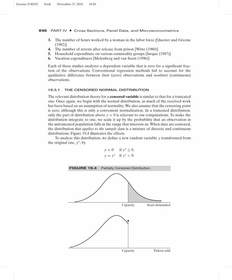
The relevant distribution theory for a censored variable is similar to that for a truncatedone. Once again, we begin with the normal distribution, as much of the received workhas been based on an assumption of normality. We also assume that the censoring pointis zero, although this is only a convenient normalization. In a truncated distribution,only the part of distribution above y = 0 is relevant to our computations. To make thedistribution integrate to one, we scale it up by the probability that an observation inthe untruncated population falls in the range that interests us. When data are censored,the distribution that applies to the sample data is a mixture of discrete and continuousdistributions. Figure 19.4 illustrates the effects.
To analyze this distribution, we define a new random variable y transformed fromthe original one, y∗, by
y = 0 if y∗ ≤ 0,
y = y∗ if y∗ > 0.
FIGURE 19.4 Partially Censored Distribution.
Capacity Seats demanded
Capacity Tickets sold
Greene-2140242 book November 27, 2010 18:36
CHAPTER 19 ✦ Limited Dependent Variables 847
The distribution that applies if y∗ ∼ N[μ, σ 2] is Prob(y = 0) = Prob(y∗ ≤ 0) =�(−μ/σ) = 1 − �(μ/σ), and if y∗ > 0, then y has the density of y∗.
This distribution is a mixture of discrete and continuous parts. The total probabilityis one, as required, but instead of scaling the second part, we simply assign the fullprobability in the censored region to the censoring point, in this case, zero.
THEOREM 19.3 Moments of the Censored Normal VariableIf y∗ ∼ N[μ, σ 2] and y = a if y∗ ≤ a or else y = y∗, then
E [y] = �a + (1 − �)(μ + σλ),
and
Var[y] = σ 2(1 − �)[(1 − δ) + (α − λ)2�],
where
�[(a − μ)/σ ] = �(α) = Prob(y∗ ≤ a) = �, λ = φ/(1 − �),
and
δ = λ2 − λα.
Proof: For the mean,
E [y] = Prob(y = a) × E [y | y = a] + Prob(y > a) × E [y | y > a]
= Prob(y∗ ≤ a) × a + Prob(y∗ > a) × E [y∗ | y∗ > a]
= �a + (1 − �)(μ + σλ)
using Theorem 19.2. For the variance, we use a counterpart to the decompositionin (B-69), that is, Var[y] = E [conditional variance] + Var[conditional mean],and Theorem 19.2.
For the special case of a = 0, the mean simplifies to
E [y | a = 0] = �(μ/σ)(μ + σλ), where λ = φ(μ/σ)
�(μ/σ).
For censoring of the upper part of the distribution instead of the lower, it is only neces-sary to reverse the role of � and 1 − � and redefine λ as in Theorem 19.2.
Example 19.4 Censored Random VariableWe are interested in the number of tickets demanded for events at a certain arena. Our onlymeasure is the number actually sold. Whenever an event sells out, however, we know that theactual number demanded is larger than the number sold. The number of tickets demandedis censored when it is transformed to obtain the number sold. Suppose that the arena inquestion has 20,000 seats and, in a recent season, sold out 25 percent of the time. If theaverage attendance, including sellouts, was 18,000, then what are the mean and standarddeviation of the demand for seats? According to Theorem 19.3, the 18,000 is an estimate of
E [sales] = 20,000(1 − �) + [μ + σλ]�.
Because this is censoring from above, rather than below, λ = −φ (α)/�(α) . The argu-ment of �, φ, and λ is α = (20,000 − μ)/σ . If 25 percent of the events are sellouts, then� = 0.75. Inverting the standard normal at 0.75 gives α = 0.675. In addition, if α = 0.675,
Greene-2140242 book November 27, 2010 18:36
848 PART IV ✦ Cross Sections, Panel Data, and Microeconometrics
then −φ (0.675)/0.75 = λ = − 0.424. This result provides two equations in μ and σ , (a)18,000 = 0.25(20,000) + 0.75(μ − 0.424σ ) and (b) 0.675σ = 20,000 − μ. The solutions areσ = 2426 and μ = 18,362.
For comparison, suppose that we were told that the mean of 18,000 applies only to theevents that were not sold out and that, on average, the arena sells out 25 percent of thetime. Now our estimates would be obtained from the equations (a) 18,000 = μ − 0.424σ and(b) 0.675σ = 20,000 − μ. The solutions are σ = 1820 and μ = 18,772.
19.3.2 THE CENSORED REGRESSION (TOBIT) MODEL
The regression model based on the preceding discussion is referred to as the censoredregression model or the tobit model [in reference to Tobin (1958), where the modelwas first proposed]. The regression is obtained by making the mean in the precedingcorrespond to a classical regression model. The general formulation is usually given interms of an index function,
y∗i = x′
iβ + εi ,
yi = 0 if y∗i ≤ 0,
yi = y∗i if y∗
i > 0.
There are potentially three conditional mean functions to consider, depending on thepurpose of the study. For the index variable, sometimes called the latent variable,E [y∗
i | xi ] is x′iβ. If the data are always censored, however, then this result will usu-
ally not be useful. Consistent with Theorem 19.3, for an observation randomly drawnfrom the population, which may or may not be censored,
E [yi | xi ] = �
(x′
iβ
σ
)(x′
iβ + σλi ),
where
λi = φ[(0 − x′iβ)/σ ]
1 − �[(0 − x′iβ)/σ ]
= φ(x′iβ/σ)
�(x′iβ/σ)
. (19-12)
Finally, if we intend to confine our attention to uncensored observations, then the re-sults for the truncated regression model apply. The limit observations should not bediscarded, however, because the truncated regression model is no more amenable toleast squares than the censored data model. It is an unresolved question which of thesefunctions should be used for computing predicted values from this model. Intuitionsuggests that E [yi | xi ] is correct, but authors differ on this point. For the setting inExample 19.4, for predicting the number of tickets sold, say, to plan for an upcomingevent, the censored mean is obviously the relevant quantity. On the other hand, if theobjective is to study the need for a new facility, then the mean of the latent variable y∗
iwould be more interesting.
There are differences in the partial effects as well. For the index variable,
∂E [y∗i | xi ]
∂xi= β.
But this result is not what will usually be of interest, because y∗i is unobserved. For the
observed data, yi , the following general result will be useful:10
10See Greene (1999) for the general result and Rosett and Nelson (1975) and Nakamura and Nakamura(1983) for applications based on the normal distribution.
Greene-2140242 book November 27, 2010 18:36
CHAPTER 19 ✦ Limited Dependent Variables 849
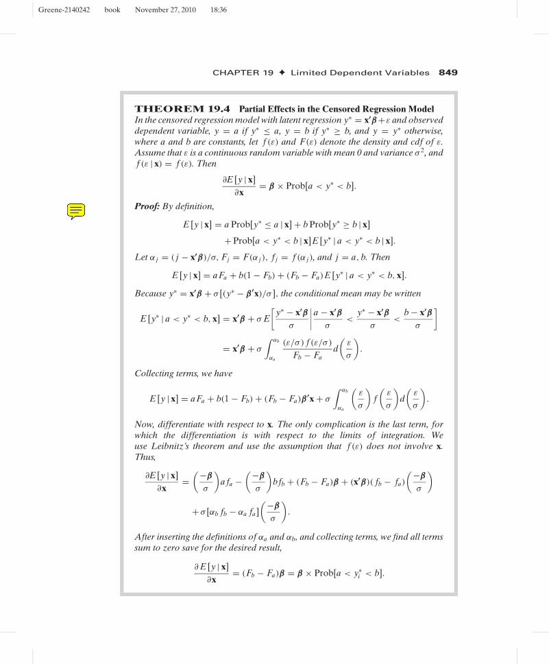
THEOREM 19.4 Partial Effects in the Censored Regression ModelIn the censored regression model with latent regression y∗ = x′β+ε and observeddependent variable, y = a if y∗ ≤ a, y = b if y∗ ≥ b, and y = y∗ otherwise,where a and b are constants, let f (ε) and F(ε) denote the density and cdf of ε.Assume that ε is a continuous random variable with mean 0 and variance σ 2, andf (ε | x) = f (ε). Then
∂E [y | x]∂x
= β × Prob[a < y∗ < b].
Proof: By definition,
E [y | x] = a Prob[y∗ ≤ a | x] + b Prob[y∗ ≥ b | x]
+ Prob[a < y∗ < b | x]E [y∗ | a < y∗ < b | x].
Let α j = ( j − x′β)/σ, Fj = F(α j ), f j = f (α j ), and j = a, b. Then
E [y | x] = aFa + b(1 − Fb) + (Fb − Fa)E [y∗ | a < y∗ < b, x].
Because y∗ = x′β + σ [(y∗ − β ′x)/σ ], the conditional mean may be written
E [y∗ | a < y∗ < b, x] = x′β + σ E[
y∗ − x′βσ
∣∣∣∣a − x′βσ
<y∗ − x′β
σ<
b − x′βσ
]
= x′β + σ
∫ αb
αa
(ε/σ ) f (ε/σ )
Fb − Fad(
ε
σ
).
Collecting terms, we have
E [y | x] = aFa + b(1 − Fb) + (Fb − Fa)β′x + σ
∫ αb
αa
(ε
σ
)f(
ε
σ
)d(
ε
σ
).
Now, differentiate with respect to x. The only complication is the last term, forwhich the differentiation is with respect to the limits of integration. Weuse Leibnitz’s theorem and use the assumption that f (ε) does not involve x.Thus,
∂E [y | x]∂x
=(−β
σ
)a fa −
(−β
σ
)bfb + (Fb − Fa)β + (x′β)( fb − fa)
(−β
σ
)
+ σ [αb fb − αa fa](−β
σ
).
After inserting the definitions of αa and αb, and collecting terms, we find all termssum to zero save for the desired result,
∂ E [y | x]∂x
= (Fb − Fa)β = β × Prob[a < y∗i < b].
MPS
Note
AU: We have received CE MSP in wrong sequence. Per our judgement page 19-21 s/b 19-20 and we kept complete Theorem 19.4 in one place. Plz check & suggest.

Greene-2140242 book November 27, 2010 18:36
850 PART IV ✦ Cross Sections, Panel Data, and Microeconometrics
Note that this general result includes censoring in either or both tails of the distribu-tion, and it does not assume that ε is normally distributed. For the standard case withcensoring at zero and normally distributed disturbances, the result specializes to
∂E [yi | xi ]∂xi
= β�
(x′
iβ
σ
).
Although not a formal result, this does suggest a reason why, in general, least squaresestimates of the coefficients in a tobit model usually resemble the MLEs times theproportion of nonlimit observations in the sample.
McDonald and Moffitt (1980) suggested a useful decomposition of ∂E [yi | xi ]/∂xi ,
∂E [yi | xi ]∂xi
= β × {�i [1 − λi (αi + λi )] + φi (αi + λi )
},
where αi = x′iβ/σ , �i = �(αi ) and λi = φi/�i . Taking the two parts separately, this
result decomposes the slope vector into
∂ E [yi | xi ]∂xi
= Prob[yi > 0]∂ E [yi | xi , yi > 0]
∂xi+ E [yi | xi , yi > 0]
∂ Prob[yi > 0]∂xi
.
Thus, a change in xi has two effects: It affects the conditional mean of y∗i in the positive
part of the distribution, and it affects the probability that the observation will fall inthat part of the distribution.
19.3.3 ESTIMATION
The tobit model has become so routine and been incorporated in so many computerpackages that despite formidable obstacles in years past, estimation is now essentiallyon the level of ordinary linear regression. The log-likelihood for the censored regressionmodel is
ln L =∑yi >0
−12
[log(2π) + ln σ 2 + (yi − x′
iβ)2
σ 2
]+
∑yi =0
ln[
1 − �
(x′
iβ
σ
)]. (19-13)
The two parts correspond to the classical regression for the nonlimit observations andthe relevant probabilities for the limit observations, respectively. This likelihood is anonstandard type, because it is a mixture of discrete and continuous distributions. Ina seminal paper, Amemiya (1973) showed that despite the complications, proceedingin the usual fashion to maximize ln L would produce an estimator with all the familiardesirable properties attained by MLEs.
The log-likelihood function is fairly involved, but Olsen’s (1978) reparameterizationsimplifies things considerably. With γ = β/σ and θ = 1/σ , the log-likelihood is
ln L =∑yi >0
−12
[ln(2π) − ln θ2 + (θyi − x′iγ )2] +
∑yi =0
ln[1 − �(x′iγ )]. (19-14)
The results in this setting are now very similar to those for the truncated regression.The Hessian is always negative definite, so Newton’s method is simple to use andusually converges quickly. After convergence, the original parameters can be recov-ered using σ = 1/θ and β = γ /θ . The asymptotic covariance matrix for these esti-mates can be obtained from that for the estimates of [γ , θ ] using the delta method:
Greene-2140242 book November 27, 2010 18:36
CHAPTER 19 ✦ Limited Dependent Variables 851
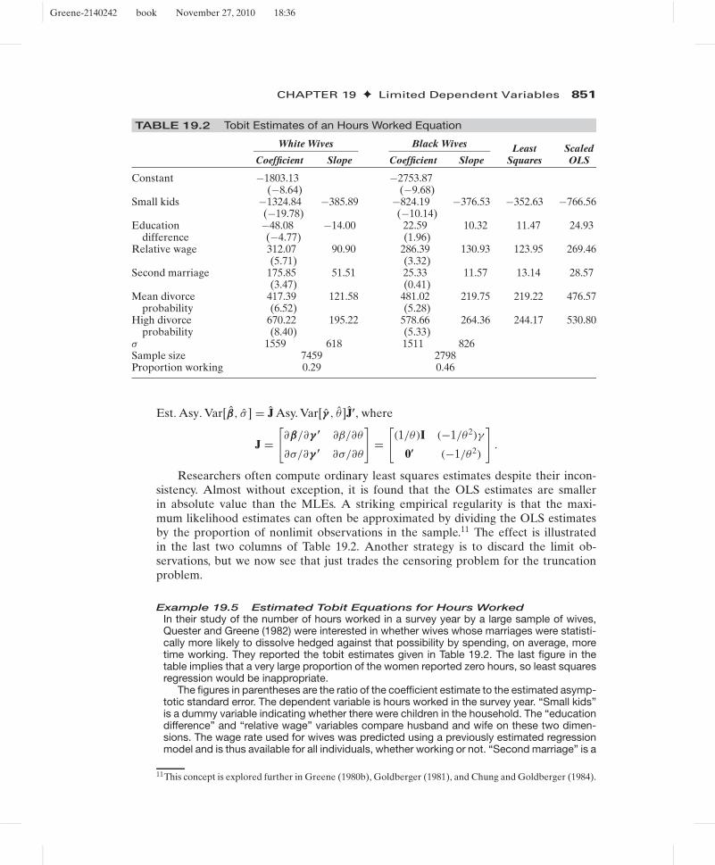
TABLE 19.2 Tobit Estimates of an Hours Worked Equation
White Wives Black Wives
Coefficient Slope Coefficient SlopeLeast
SquaresScaledOLS
Constant −1803.13 −2753.87(−8.64) (−9.68)
Small kids −1324.84 −385.89 −824.19 −376.53 −352.63 −766.56(−19.78) (−10.14)
Education −48.08 −14.00 22.59 10.32 11.47 24.93difference (−4.77) (1.96)
Relative wage 312.07 90.90 286.39 130.93 123.95 269.46(5.71) (3.32)
Second marriage 175.85 51.51 25.33 11.57 13.14 28.57(3.47) (0.41)
Mean divorce 417.39 121.58 481.02 219.75 219.22 476.57probability (6.52) (5.28)
High divorce 670.22 195.22 578.66 264.36 244.17 530.80probability (8.40) (5.33)
σ 1559 618 1511 826Sample size 7459 2798Proportion working 0.29 0.46
Est. Asy. Var[β, σ ] = J Asy. Var[γ , θ ]J′, where
J =[∂β/∂γ ′ ∂β/∂θ
∂σ/∂γ ′ ∂σ/∂θ
]=
[(1/θ)I (−1/θ2)γ
0′ (−1/θ2)
].
Researchers often compute ordinary least squares estimates despite their incon-sistency. Almost without exception, it is found that the OLS estimates are smallerin absolute value than the MLEs. A striking empirical regularity is that the maxi-mum likelihood estimates can often be approximated by dividing the OLS estimatesby the proportion of nonlimit observations in the sample.11 The effect is illustratedin the last two columns of Table 19.2. Another strategy is to discard the limit ob-servations, but we now see that just trades the censoring problem for the truncationproblem.
Example 19.5 Estimated Tobit Equations for Hours WorkedIn their study of the number of hours worked in a survey year by a large sample of wives,Quester and Greene (1982) were interested in whether wives whose marriages were statisti-cally more likely to dissolve hedged against that possibility by spending, on average, moretime working. They reported the tobit estimates given in Table 19.2. The last figure in thetable implies that a very large proportion of the women reported zero hours, so least squaresregression would be inappropriate.
The figures in parentheses are the ratio of the coefficient estimate to the estimated asymp-totic standard error. The dependent variable is hours worked in the survey year. “Small kids”is a dummy variable indicating whether there were children in the household. The “educationdifference” and “relative wage” variables compare husband and wife on these two dimen-sions. The wage rate used for wives was predicted using a previously estimated regressionmodel and is thus available for all individuals, whether working or not. “Second marriage” is a
11This concept is explored further in Greene (1980b), Goldberger (1981), and Chung and Goldberger (1984).

Greene-2140242 book November 27, 2010 18:36
852 PART IV ✦ Cross Sections, Panel Data, and Microeconometrics
dummy variable. Divorce probabilities were produced by a large microsimulation model pre-sented in another study [Orcutt, Caldwell, and Wertheimer (1976)]. The variables used herewere dummy variables indicating “mean” if the predicted probability was between 0.01 and0.03 and “high” if it was greater than 0.03. The “slopes” are the marginal effects describedearlier.
Note the marginal effects compared with the tobit coefficients. Likewise, the estimate ofσ is quite misleading as an estimate of the standard deviation of hours worked.
The effects of the divorce probability variables were as expected and were quite large. Oneof the questions raised in connection with this study was whether the divorce probabilitiescould reasonably be treated as independent variables. It might be that for these individuals,the number of hours worked was a significant determinant of the probability.
19.3.4 TWO-PART MODELS AND CORNER SOLUTIONS
The tobit model contains a restriction that might be unreasonable in an economic setting.Consider a behavioral outcome, y = charitable donation. Two implications of the tobitmodel are that
Prob(y > 0 | x) = Prob(x′β + ε > 0 | x) = �(x′β/σ)
and [from (19-7)]
E[y | y > 0, x] = x′β + σφ(x′β/σ)/�(x′β/σ).
Differentiating both of these, we find from (17-11) and (19-8),
∂Prob(y > 0 | x)/∂x = [φ(x′β/σ)/σ ]β = a positive multiple of β,
∂ E[y | y > 0, x]/∂x = {[1 − δ(x′β/σ)]/σ }β = a positive multiple of β.
Thus, any variable that appears in the model affects the participation probability and theintensity equation with the same sign. In the case suggested, for example, it is conceivablethat age might affect participation and intensity in different directions. Fin and Schmidt(1984) suggest another application, loss due to fire in buildings; older buildings might bemore likely to have fires but, because of the greater value of newer buildings, the actualdamage might be greater in newer buildings. This fact would require the coefficient onage to have different signs in the two functions, which is impossible in the tobit modelbecause they are the same coefficient.
In an early study in this literature, Cragg (1971) proposed a somewhat more generalmodel in which the probability of a limit observation is independent of the regressionmodel for the nonlimit data. One can imagine, for instance, the decision of whether ornot to purchase a car as being different from the decision of how much to spend on thecar, having decided to buy one.
A more general model that accommodates these objections is as follows:
1. Participation equation
Prob[y∗i > 0] = �(x′
iγ ), di = 1 if y∗i > 0,
Prob[y∗i ≤ 0] = 1 − �(x′
iγ ), di = 0 if y∗i ≤ 0.
(19-15)
2. Intensity equation for nonlimit observations
E[yi | di = 1] = x′iβ + σλi ,

Greene-2140242 book November 27, 2010 18:36
CHAPTER 19 ✦ Limited Dependent Variables 853
according to Theorem 19.2. This two-part model is a combination of the truncated re-gression model of Section 19.2 and the univariate probit model of Section 17.3, whichsuggests a method of analyzing it. Note that it is precisely the same approach we con-sidered in Section 18.4.8 and Example 18.12 where we used a hurdle model to modeldoctor visits. The tobit model returns if γ = β/σ . The parameters of the regression (in-tensity) equation can be estimated independently using the truncated regression modelof Section 19.2. An application is Melenberg and van Soest (1996).
Lin and Schmidt (1984) considered testing the restriction of the tobit model. Basedonly on the tobit model, they devised a Lagrange multiplier statistic that, although abit cumbersome algebraically, can be computed without great difficulty. If one is ableto estimate the truncated regression model, the tobit model, and the probit modelseparately, then there is a simpler way to test the hypothesis. The tobit log-likelihoodis the sum of the log-likelihoods for the truncated regression and probit models. Toshow this result, add and subtract
∑yi =1 ln �(x′
iβ) in (19-13). This produces the log-likelihood for the truncated regression model (considered in the exercises) plus (17-20)for the probit model. Therefore, a likelihood ratio statistic can be computed using
λ = −2[ln LT − (ln LP + ln LTR)],
where
LT = likelihood for the tobit model in (19-13), with the same coefficients
LP = likelihood for the probit model in (17-17), fit separately
LTR = likelihood for the truncated regression model, fit separately
The two-part model just considered extends the tobit model, but it stops a bit shortof the generality we might achieve. In the preceding hurdle model, we have assumedthat the same regressors appear in both equations. Although this produces a convenientway to retreat to the tobit model as a parametric restriction, it couples the two decisionsperhaps unreasonably. In our example to follow, where we model extramarital affairs,the decision whether or not to spend any time in an affair may well be an entirelydifferent decision from how much time to spend having once made that commitment.The obvious way to proceed is to reformulate the hurdle model as
1. Participation equation
Prob[d∗i > 0] = �(z′
iγ ), di = 1 if d∗i > 0,
Prob[d∗i ≤ 0] = 1 − �(z′
iγ ), di = 0 if d∗i ≤ 0. (19-16)
2. Intensity equation for nonlimit observations
E[yi | di = 1] = x′iβ + σλi .
This extension, however, omits an important element; it seems unlikely that the twodecisions would be uncorrelated; that is, the implicit disturbances in the equations shouldbe correlated. The combination of these produces what has been labeled a type-II tobitmodel. [Amemiya (1985) identified five possible permutations of the model specificationand observation mechanism. The familiar tobit model is type I; this is type-II.] The fullmodel is

Greene-2140242 book November 27, 2010 18:36
854 PART IV ✦ Cross Sections, Panel Data, and Microeconometrics
1. Participation equation
d∗i = z′
iγ + ui , ui ∼ N[0, 1]
di = 1 if d∗i > 0, 0 otherwise.
2. Intensity equation
y∗i = x′
iβ + εi , εi ∼ N[0, σ 2].
3. Observation mechanism
(a) y∗i = 0 if di = 0 and yi = y∗
i if di = 1.
(b) yi = y∗i if di = 1 and yi is unobserved if di = 0.
4. Endogeneity
(ui , εi ) ∼ bivariate normal with correlation ρ.
Mechanism (a) produces Amemiya’s type II model. (Amemiya blends these two in-terpretations. In the statement of the model, he presents (a), but in the subsequentdiscussion, assumes (b). The difference is substantive if xi is observed in case (b). Oth-erwise, they are the same, and “yi = 0” is not actually meaningful. Amemiya notes,“y∗
i = 0 merely signifies the event d∗i ≤ 0.” If xi is observed when di = 0, then these ob-
servations will contribute to the likelihood for the full sample. If not, then they will not.We will develop this idea later when we consider Heckman’s selection model [which iscase (b) without observed xi when di = 0].
There are two estimation strategies that can be used to fit the type II model. A two-step method can proceed as follows: The probit model for di can be estimated usingmaximum likelihood as shown in Section 17.3. For the second step, we make use of ourtheorems on truncation (and Theorem 19.5 that will appear later) to write
E[yi | di = 1, xi , zi ] = x′iβ + E[εi | di = 1, xi , zi ]
= x′iβ + ρσ
φ(z′iγ )
�(z′iγ )
(19-17)
= x′iβ + ρσλi .
Since we have estimated γ at step 1, we can compute λi = φ(z′i γ )/�(z′
i γ ) using thefirst-step estimates, and we can estimate β and θ = (ρσ) by least squares regression ofyi on xi and λi . It will be necessary to correct the asymptotic covariance matrix thatis computed for (β, θ ). This is a template application of the Murphy and Topel (2002)results that appear in Section 14.7. The second approach is full information maximumlikelihood, estimating all the parameters in both equations simultaneously. We willreturn to the details of estimation of the type II tobit model in Section 19.5 wherewe examine Heckman’s model of “sample selection” model (which is the type II tobitmodel).
Many of the applications of the tobit model in the received literature are con-structed not to accommodate censoring of the underlying data, but, rather, to modelthe appearance of a large cluster of zeros. Cragg’s application is clearly related to thisphenomenon. Consider, for example, survey data on purchases of consumer durables,firm expenditure on research and development, or consumer savings. In each case, the

Greene-2140242 book November 27, 2010 18:36
CHAPTER 19 ✦ Limited Dependent Variables 855
0.000 14.131 28.262 42.393
Freq
uenc
y
56.524SPENDING
70.655 84.786 98.917
FIGURE 19.5 Hypothetical Spending Data.
observed data will consist of zero or some positive amount. Arguably, there are twodecisions at work in these scenarios: First, whether to engage in the activity or not, andsecond, given that the answer to the first question is yes, how intensively to engage init—how much to spend, for example. This is precisely the motivation behind the hurdlemodel. This specification has been labeled a “corner solution model”; see Wooldridge(2002a, pp. 518–519).
In practical terms, the difference between the hurdle model and the tobit modelshould be evident in the data. Often overlooked in tobit analyses is that the modelpredicts not only a cluster of zeros (or limit observations), but also a grouping of obser-vations near zero (or the limit point). For example, the tobit model is surely misspec-ified for the sort of (hypothetical) spending data shown in Figure 19.5 for a sample of1,000 observations. Neglecting for the moment the earlier point about the underlyingdecision process, Figure 19.6 shows the characteristic appearance of a (substantively)censored variable. The implication for the model builder is that an appropriate speci-fication would consist of two equations, one for the “participation decision,” and onefor the distribution of the positive dependent variable. Formally, we might, continuingthe development of Cragg’s specification, model the first decision with a binary choice(e.g., probit or logit model). The second equation is a model for y | y > 0, for whichthe truncated regression model of Section 19.2.3 is a natural candidate. As we willsee, this is essentially the model behind the sample selection treatment developed inSection 19.5.
Two practical issues frequently intervene at this point. First, one might well havea model in mind for the intensity (regression) equation, but none for the participationequation. This is the usual backdrop for the uses of the tobit model, which produces theconsiderations in the previous section. The second issue concerns the appropriateness

Greene-2140242 book November 27, 2010 18:36
856 PART IV ✦ Cross Sections, Panel Data, and Microeconometrics
0.000 9.862 19.723 29.585
Freq
uenc
y
39.446SPENDING
49.308 59.169 69.031
FIGURE 19.6 Hypothetical Censored Data.
of the truncation or censoring model to data such as those in Figure 19.6. If we consideronly the nonlimit observations in Figure 19.5, the underlying distribution does notappear to be truncated at all. The truncated regression model in Section 19.2.3 fit to thesedata will not depart significantly from ordinary least squares [because the underlyingprobability in the denominator of (19-6) will equal one and the numerator will equalzero]. But, this is not the case of a tobit model forced on these same data. Forcingthe model in (19-13) on data such as these will significantly distort the estimator—allelse equal, it will significantly attenuate the coefficients, the more so the larger is theproportion of limit observations in the sample. Once again, this stands as a caveat forthe model builder. The tobit model is manifestly misspecified for data such as those inFigure 19.5.
Example 19.6 Two-Part Model for Extramarital AffairsIn Example 18.9, we examined Fair’s (1977) Psychology Today survey data on extramaritalaffairs. The 601 observations in the data set are mostly zero—451 of the 601. This featureof the data motivated the author to use a tobit model to analyze these data. In our example,we reconsidered the model, since the nonzero observations were a count, not a continuousvariable. Another data set in Fair’s study was the Redbook Magazine survey of 6,366 marriedwomen. Once again, the outcome variable of interest was extramarital affairs. However, inthis instance, the outcome data were transformed to a measure of time spent, which, beingcontinuous, lends itself more naturally to the tobit model we are studying here. The variablesin the data set are as follows (excluding three unidentified and not used):
id = Identification numberC = Constant, value = 1yrb = Constructed measure of time spent in extramarital affairsv1 = Rating of the marriage, coded 1 to 4v2 = Age, in years, aggregatedv3 = Number of years married
Greene-2140242 book November 27, 2010 18:36
CHAPTER 19 ✦ Limited Dependent Variables 857
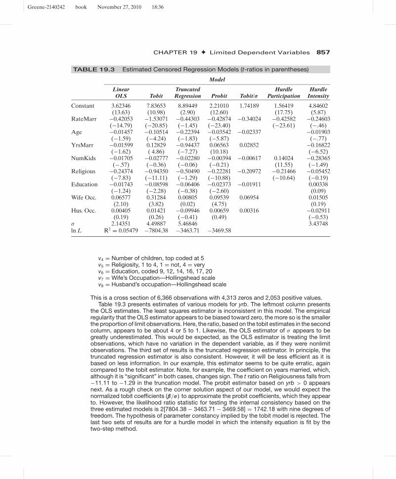
TABLE 19.3 Estimated Censored Regression Models (t-ratios in parentheses)
Model
Linear Truncated Hurdle HurdleOLS Tobit Regression Probit Tobit/σ Participation Intensity
Constant 3.62346 7.83653 8.89449 2.21010 1.74189 1.56419 4.84602(13.63) (10.98) (2.90) (12.60) (17.75) (5.87)
RateMarr −0.42053 −1.53071 −0.44303 −0.42874 −0.34024 −0.42582 −0.24603(−14.79) (−20.85) (−1.45) (−23.40) (−23.61) (−.46)
Age −0.01457 −0.10514 −0.22394 −0.03542 −0.02337 −0.01903(−1.59) (−4.24) (−1.83) (−5.87) (−.77)
YrsMarr −0.01599 0.12829 −0.94437 0.06563 0.02852 −0.16822(−1.62) ( 4.86) (−7.27) (10.18) (−6.52)
NumKids −0.01705 −0.02777 −0.02280 −0.00394 −0.00617 0.14024 −0.28365(−.57) (−0.36) (−0.06) (−0.21) (11.55) (−1.49)
Religious −0.24374 −0.94350 −0.50490 −0.22281 −0.20972 −0.21466 −0.05452(−7.83) (−11.11) (−1.29) (−10.88) (−10.64) (−0.19)
Education −0.01743 −0.08598 −0.06406 −0.02373 −0.01911 0.00338(−1.24) (−2.28) (−0.38) (−2.60) (0.09)
Wife Occ. 0.06577 0.31284 0.00805 0.09539 0.06954 0.01505(2.10) (3.82) (0.02) (4.75) (0.19)
Hus. Occ. 0.00405 0.01421 −0.09946 0.00659 0.00316 −0.02911(0.19) (0.26) (−0.41) (0.49) (−0.53)
σ 2.14351 4.49887 5.46846 3.43748ln L R2 = 0.05479 −7804.38 −3463.71 −3469.58
v4 = Number of children, top coded at 5v5 = Religiosity, 1 to 4, 1 = not, 4 = veryv6 = Education, coded 9, 12, 14, 16, 17, 20v7 = Wife’s Occupation—Hollingshead scalev8 = Husband’s occupation—Hollingshead scale
This is a cross section of 6,366 observations with 4,313 zeros and 2,053 positive values.Table 19.3 presents estimates of various models for yrb. The leftmost column presents
the OLS estimates. The least squares estimator is inconsistent in this model. The empiricalregularity that the OLS estimator appears to be biased toward zero, the more so is the smallerthe proportion of limit observations. Here, the ratio, based on the tobit estimates in the secondcolumn, appears to be about 4 or 5 to 1. Likewise, the OLS estimator of σ appears to begreatly underestimated. This would be expected, as the OLS estimator is treating the limitobservations, which have no variation in the dependent variable, as if they were nonlimitobservations. The third set of results is the truncated regression estimator. In principle, thetruncated regression estimator is also consistent. However, it will be less efficient as it isbased on less information. In our example, this estimator seems to be quite erratic, againcompared to the tobit estimator. Note, for example, the coefficient on years married, which,although it is “significant” in both cases, changes sign. The t ratio on Religiousness falls from−11.11 to −1.29 in the truncation model. The probit estimator based on yrb > 0 appearsnext. As a rough check on the corner solution aspect of our model, we would expect thenormalized tobit coefficients (β/σ ) to approximate the probit coefficients, which they appearto. However, the likelihood ratio statistic for testing the internal consistency based on thethree estimated models is 2[7804.38 − 3463.71 − 3469.58] = 1742.18 with nine degrees offreedom. The hypothesis of parameter constancy implied by the tobit model is rejected. Thelast two sets of results are for a hurdle model in which the intensity equation is fit by thetwo-step method.

Greene-2140242 book November 27, 2010 18:36
858 PART IV ✦ Cross Sections, Panel Data, and Microeconometrics
19.3.5 SOME ISSUES IN SPECIFICATION
Two issues that commonly arise in microeconomic data, heteroscedasticity and nonnor-mality, have been analyzed at length in the tobit setting.12
19.3.5.a Heteroscedasticity
Maddala and Nelson (1975), Hurd (1979), Arabmazar and Schmidt (1982a,b), andBrown and Moffitt (1982) all have varying degrees of pessimism regarding how in-consistent the maximum likelihood estimator will be when heteroscedasticity occurs.Not surprisingly, the degree of censoring is the primary determinant. Unfortunately, allthe analyses have been carried out in the setting of very specific models—for example,involving only a single dummy variable or one with groupwise heteroscedasticity—sothe primary lesson is the very general conclusion that heteroscedasticity emerges as anobviously serious problem.
One can approach the heteroscedasticity problem directly. Petersen and Waldman(1981) present the computations needed to estimate a tobit model with heteroscedastic-ity of several types. Replacing σ with σi in the log-likelihood function and including σ 2
iin the summations produces the needed generality. Specification of a particular modelfor σi provides the empirical model for estimation.
Example 19.7 Multiplicative Heteroscedasticity in the Tobit ModelPetersen and Waldman (1981) analyzed the volume of short interest in a cross section ofcommon stocks. The regressors included a measure of the market component of heteroge-neous expectations as measured by the firm’s BETA coefficient; a company-specific measureof heterogeneous expectations, NONMARKET; the NUMBER of analysts making earningsforecasts for the company; the number of common shares to be issued for the acquisitionof another firm, MERGER; and a dummy variable for the existence of OPTIONs. They reportthe results listed in Table 19.4 for a model in which the variance is assumed to be of the formσ 2
i = exp(x′i α) . The values in parentheses are the ratio of the coefficient to the estimated
asymptotic standard error.The effect of heteroscedasticity on the estimates is extremely large. We do note, however,
a common misconception in the literature. The change in the coefficients is often misleading.The marginal effects in the heteroscedasticity model will generally be very similar to thosecomputed from the model which assumes homoscedasticity. (The calculation is pursued inthe exercises.)
A test of the hypothesis that α = 0 (except for the constant term) can be based on thelikelihood ratio statistic. For these results, the statistic is −2[−547.3 − (−466.27) ] = 162.06.This statistic has a limiting chi-squared distribution with five degrees of freedom. The samplevalue exceeds the critical value in the table of 11.07, so the hypothesis can be rejected.
In the preceding example, we carried out a likelihood ratio test against the hypoth-esis of homoscedasticity. It would be desirable to be able to carry out the test withouthaving to estimate the unrestricted model. A Lagrange multiplier test can be used for
12Two symposia that contain numerous results on these subjects are Blundell (1987) and Duncan (1986b).An application that explores these two issues in detail is Melenberg and van Soest (1996). Developing speci-fication tests for the tobit model has been a popular enterprise. A sampling of the received literature includesNelson (1981); Bera, Jarque, and Lee (1982); Chesher and Irish (1987); Chesher, Lancaster, and Irish (1985);Gourieroux et al. (1984, 1987); Newey (1986); Rivers andVuong (1988); Horowitz and Neumann (1989); andPagan and Vella (1989). Newey (1985a,b) are useful references on the general subject of conditional momenttesting. More general treatments of specification testing are Godfrey (1988) and Ruud (1984).

Greene-2140242 book November 27, 2010 18:36
CHAPTER 19 ✦ Limited Dependent Variables 859
TABLE 19.4 Estimates of a Tobit Model (standard errorsin parentheses)
Homoscedastic Heteroscedastic
β β α
Constant −18.28 (5.10) −4.11 (3.28) −0.47 (0.60)Beta 10.97 (3.61) 2.22 (2.00) 1.20 (1.81)Nonmarket 0.65 (7.41) 0.12 (1.90) 0.08 (7.55)Number 0.75 (5.74) 0.33 (4.50) 0.15 (4.58)Merger 0.50 (5.90) 0.24 (3.00) 0.06 (4.17)Option 2.56 (1.51) 2.96 (2.99) 0.83 (1.70)ln L −547.30 −466.27Sample size 200 200
that purpose. Consider the heteroscedastic tobit model in which we specify that
σ 2i = σ 2[exp(w′
iα)]2. (19-18)
This model is a fairly general specification that includes many familiar ones as specialcases. The null hypothesis of homoscedasticity is α = 0. (We used this specification in theprobit model in Section 17.3.7 and in the linear regression model in Section 9.7.1) Usingthe BHHH estimator of the Hessian as usual, we can produce a Lagrange multiplierstatistic as follows: Let zi = 1 if yi is positive and 0 otherwise,
ai = zi
(εi
σ 2
)+ (1 − zi )
((−1)λi
σ
),
bi = zi
((ε2
i /σ2 − 1
)2σ 2
)+ (1 − zi )
((x′
iβ)λi
2σ 3
), (19-19)
λi = φ(x′iβ/σ)
1 − �(x′iβ/σ)
.
The data vector is gi = [ai x′i , bi , bi w′
i ]′. The sums are taken over all observations, and
all functions involving unknown parameters (εi , φi , �i , x′iβ, σ, λi ) are evaluated at the
restricted (homoscedastic) maximum likelihood estimates. Then,
LM = i′G[G′G]−1G′i = nR2 (19-20)
in the regression of a column of ones on the K + 1 + P derivatives of the log-likelihoodfunction for the model with multiplicative heteroscedasticity, evaluated at the estimatesfrom the restricted model. (If there were no limit observations, then it would reduce tothe Breusch–Pagan statistic discussed in Section 9.5.2.) Given the maximum likelihoodestimates of the tobit model coefficients, it is quite simple to compute. The statistichas a limiting chi-squared distribution with degrees of freedom equal to the number ofvariables in wi .
19.3.5.b Nonnormality
Nonnormality is an especially difficult problem in this setting. It has been shown thatif the underlying disturbances are not normally distributed, then the estimator based
Greene-2140242 book November 27, 2010 18:36
860 PART IV ✦ Cross Sections, Panel Data, and Microeconometrics
on (19-13) is inconsistent. Research is ongoing both on alternative estimators and onmethods for testing for this type of misspecification.13
One approach to the estimation is to use an alternative distribution. Kalbfleisch andPrentice (2002) present a unifying treatment that includes several distributions such asthe exponential, lognormal, and Weibull. (Their primary focus is on survival analysisin a medical statistics setting, which is an interesting convergence of the techniques invery different disciplines.) Of course, assuming some other specific distribution does notnecessarily solve the problem and may make it worse. A preferable alternative wouldbe to devise an estimator that is robust to changes in the distribution. Powell’s (1981,1984) least absolute deviations (LAD) estimator appears to offer some promise.14 Themain drawback to its use is its computational complexity. An extensive application ofthe LAD estimator is Melenberg and van Soest (1996). Although estimation in thenonnormal case is relatively difficult, testing for this failure of the model is worthwhileto assess the estimates obtained by the conventional methods. Among the tests thathave been developed are Hausman tests, Lagrange multiplier tests [Bera and Jarque(1981, 1982), Bera, Jarque, and Lee (1982)], and conditional moment tests [Nelson(1981)].
19.3.6 PANEL DATA APPLICATIONS
Extension of the familiar panel data results to the tobit model parallel the probit model,with the attendant problems. The random effects or random parameters models dis-cussed in Chapter 17 can be adapted to the censored regression model using simulationor quadrature. The same reservations with respect to the orthogonality of the effects andthe regressors will apply here, as will the applicability of the Mundlak (1978) correctionto accommodate it.
Most of the attention in the theoretical literature on panel data methods for the tobitmodel has been focused on fixed effects. The departure point would be the maximumlikelihood estimator for the static fixed effects model,
y∗it = αi + x′
itβ + εit, εit ∼ N[0, σ 2],
yit = Max(0, yit).
However, there are no firm theoretical results on the behavior of the MLE in thismodel. Intuition might suggest, based on the findings for the binary probit model, thatthe MLE would be biased in the same fashion, away from zero. Perhaps surprisingly, theresults in Greene (2004) persistently found that not to be the case in a variety of modelspecifications. Rather, the incidental parameters, such as it is, manifests in a downwardbias in the estimator of σ , not an upward (or downward) bias in the MLE of β. However,this is less surprising when the tobit estimator is juxtaposed with the MLE in the linearregression model with fixed effects. In that model, the MLE is the within-groups (LSDV)estimator which is unbiased and consistent. But, the ML estimator of the disturbancevariance in the linear regression model is e′
LSDVeLSDV/(nT ), which is biased downward
13See Duncan (1983, 1986b), Goldberger (1983), Pagan and Vella (1989), Lee (1996), and Fernandez (1986).14See Duncan (1986a,b) for a symposium on the subject and Amemiya (1984). Additional references areNewey, Powell, and Walker (1990); Lee (1996); and Robinson (1988).
Greene-2140242 book November 27, 2010 18:36
CHAPTER 19 ✦ Limited Dependent Variables 861
by a factor of (T −1)/T. [This is the result found in the original source on the incidentalparameters problem, Neyman and Scott (1948).] So, what evidence there is suggeststhat unconditional estimation of the tobit model behaves essentially like that for thelinear regression model. That does not settle the problem, however; if the evidence iscorrect, then it implies that although consistent estimation of β is possible, appropriatestatistical inference is not. The bias in the estimation of σ shows up in any estimator ofthe asymptotic covariance of the MLE of β.
Unfortunately, there is no conditional estimator of β for the tobit (or truncated re-gression) model. First differencing or taking group mean deviations does not preservethe model. Because the latent variable is censored before observation, these transforma-tions are not meaningful. Some progress has been made on theoretical, semiparametricestimators for this model. See, for example, Honore and Kyriazidou (2000) for a survey.Much of the theoretical development has also been directed at dynamic models wherethe benign result of the previous paragraph (such as it is) is lost once again. Arellano(2001) contains some general results. Hahn and Kuersteiner (2004) have characterizedthe bias of the MLE, and suggested methods of reducing the bias of the estimators indynamic binary choice and censored regression models.
19.4 MODELS FOR DURATION
The leading application of the censoring models we examined in Section 19.3 is modelsfor durations and events. We consider the time until some kind of transition as theduration, and the transition, itself, as the event. The length of a spell of unemployment(until rehire or exit from the market), the duration of a strike, the amount of time untila patient ends a health-related spell in connection with a disease or operation, and thelength of time between origination and termination (via prepayment, default, or someother mechanism) of a mortgage are all examples of durations and transitions. Therole that censoring plays in these scenarios is that in almost all cases in which we asanalysts study duration data, some or even many of the spells we observe do not endin transitions. For example, in studying the lengths of unemployment spells, many ofthe individuals in the sample may still be unemployed at the time the study ends—theanalyst observes (or believes) that the spell will end some time after the observationwindow closes. These data on spell lengths are, by construction, censored. Models ofduration will generally account explicitly for censoring of the duration data.
This section is concerned with models of duration. In some aspects, the regression-like models we have studied, such as the discrete choice models, are the appropriatetools. As in the previous two chapters, however, the models are nonlinear, and the famil-iar regression methods are not appropriate. Most of this analysis focuses on maximumlikelihood estimators. In modeling duration, although an underlying regression modelis, in fact, at work, it is generally not the conditional mean function that is of interest.More likely, as we will explore next, the objects of estimation are certain probabilitiesof events, for example in the conditional probability of a transition in a given intervalgiven that the spell has lasted up to the point of interest. These are known as “hazardmodels”—the probability is labeled the hazard function—and are a central focus of thistype of analysis.
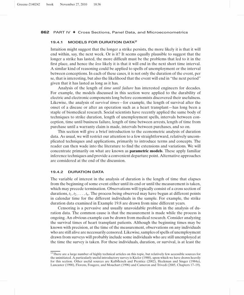
Greene-2140242 book November 27, 2010 18:36
862 PART IV ✦ Cross Sections, Panel Data, and Microeconometrics
19.4.1 MODELS FOR DURATION DATA15
Intuition might suggest that the longer a strike persists, the more likely it is that it willend within, say, the next week. Or is it? It seems equally plausible to suggest that thelonger a strike has lasted, the more difficult must be the problems that led to it in thefirst place, and hence the less likely it is that it will end in the next short time interval.A similar kind of reasoning could be applied to spells of unemployment or the intervalbetween conceptions. In each of these cases, it is not only the duration of the event, perse, that is interesting, but also the likelihood that the event will end in “the next period”given that it has lasted as long as it has.
Analysis of the length of time until failure has interested engineers for decades.For example, the models discussed in this section were applied to the durability ofelectric and electronic components long before economists discovered their usefulness.Likewise, the analysis of survival times—for example, the length of survival after theonset of a disease or after an operation such as a heart transplant—has long been astaple of biomedical research. Social scientists have recently applied the same body oftechniques to strike duration, length of unemployment spells, intervals between con-ception, time until business failure, length of time between arrests, length of time frompurchase until a warranty claim is made, intervals between purchases, and so on.
This section will give a brief introduction to the econometric analysis of durationdata. As usual, we will restrict our attention to a few straightforward, relatively uncom-plicated techniques and applications, primarily to introduce terms and concepts. Thereader can then wade into the literature to find the extensions and variations. We willconcentrate primarily on what are known as parametric models. These apply familiarinference techniques and provide a convenient departure point. Alternative approachesare considered at the end of the discussion.
19.4.2 DURATION DATA
The variable of interest in the analysis of duration is the length of time that elapsesfrom the beginning of some event either until its end or until the measurement is taken,which may precede termination. Observations will typically consist of a cross section ofdurations, t1, t2, . . . , tn. The process being observed may have begun at different pointsin calendar time for the different individuals in the sample. For example, the strikeduration data examined in Example 19.8 are drawn from nine different years.
Censoring is a pervasive and usually unavoidable problem in the analysis of du-ration data. The common cause is that the measurement is made while the process isongoing. An obvious example can be drawn from medical research. Consider analyzingthe survival times of heart transplant patients. Although the beginning times may beknown with precision, at the time of the measurement, observations on any individualswho are still alive are necessarily censored. Likewise, samples of spells of unemploymentdrawn from surveys will probably include some individuals who are still unemployed atthe time the survey is taken. For these individuals, duration, or survival, is at least the
15There are a large number of highly technical articles on this topic, but relatively few accessible sources forthe uninitiated. A particularly useful introductory survey is Kiefer (1988), upon which we have drawn heavilyfor this section. Other useful sources are Kalbfleisch and Prentice (2002), Heckman and Singer (1984a),Lancaster (1990), Florens, Fougere, and Mouchart (1996) and Cameron and Trivedi (2005, Chapters 17–19).

Greene-2140242 book November 27, 2010 18:36
CHAPTER 19 ✦ Limited Dependent Variables 863
observed ti , but not equal to it. Estimation must account for the censored nature of thedata for the same reasons as considered in Section 19.3. The consequences of ignoringcensoring in duration data are similar to those that arise in regression analysis.
In a conventional regression model that characterizes the conditional mean andvariance of a distribution, the regressors can be taken as fixed characteristics at thepoint in time or for the individual for which the measurement is taken. When measuringduration, the observation is implicitly on a process that has been under way for aninterval of time from zero to t. If the analysis is conditioned on a set of covariates (thecounterparts to regressors) xt , then the duration is implicitly a function of the entiretime path of the variable x(t), t = (0, t), which may have changed during the interval.For example, the observed duration of employment in a job may be a function of theindividual’s rank in the firm. But their rank may have changed several times betweenthe time they were hired and when the observation was made. As such, observed rankat the end of the job tenure is not necessarily a complete description of the individual’srank while they were employed. Likewise, marital status, family size, and amount ofeducation are all variables that can change during the duration of unemployment andthat one would like to account for in the duration model. The treatment of time-varyingcovariates is a considerable complication.16
19.4.3 A REGRESSION-LIKE APPROACH: PARAMETRICMODELS OF DURATION
We will use the term spell as a catchall for the different duration variables we mightmeasure. Spell length is represented by the random variable T. A simple approach toduration analysis would be to apply regression analysis to the sample of observed spells.By this device, we could characterize the expected duration, perhaps conditioned ona set of covariates whose values were measured at the end of the period. We couldalso assume that conditioned on an x that has remained fixed from T = 0 to T = t, thas a normal distribution, as we commonly do in regression. We could then characterizethe probability distribution of observed duration times. But, normality turns out not tobe particularly attractive in this setting for a number of reasons, not least of which isthat duration is positive by construction, while a normally distributed variable can takenegative values. (lognormality turns out to be a palatable alternative, but it is only oneamong a long list of candidates.)
19.4.3.a Theoretical Background
Suppose that the random variable T has a continuous probability distribution f (t),where t is a realization of T. The cumulative probability is
F(t) =∫ t
0f (s) ds = Prob(T ≤ t).
We will usually be more interested in the probability that the spell is of length at leastt, which is given by the survival function,
S(t) = 1 − F(t) = Prob(T ≥ t).
16See Petersen (1986) for one approach to this problem.

Greene-2140242 book November 27, 2010 18:36
864 PART IV ✦ Cross Sections, Panel Data, and Microeconometrics
Consider the question raised in the introduction: Given that the spell has lasted untiltime t , what is the probability that it will end in the next short interval of time, say, �t?It is
l(t, �t) = Prob(t ≤ T ≤ t + �t | T ≥ t).
A useful function for characterizing this aspect of the distribution is the hazard rate,
λ(t) = lim�t→0
Prob(t ≤ T ≤ t + �t | T ≥ t)�t
= lim�t→0
F(t + �t) − F(t)�t S(t)
= f (t)S(t)
.
Roughly, the hazard rate is the rate at which spells are completed after duration t , giventhat they last at least until t . As such, the hazard function gives an answer to our originalquestion.
The hazard function, the density, the CDF, and the survival function are all related.The hazard function is
λ(t) = −d ln S(t)dt
,
so
f (t) = S(t)λ(t).
Another useful function is the integrated hazard function
�(t) =∫ t
0λ(s) ds,
for which
S(t) = e−�(t),
so
�(t) = −ln S(t).
The integrated hazard function is generalized residual in this setting. [See Chesher andIrish (1987) and Example 19.8.]
19.4.3.b Models of the Hazard Function
For present purposes, the hazard function is more interesting than the survival rateor the density. Based on the previous results, one might consider modeling the hazardfunction itself, rather than, say, modeling the survival function and then obtaining thedensity and the hazard. For example, the base case for many analyses is a hazard ratethat does not vary over time. That is, λ(t) is a constant λ. This is characteristic of aprocess that has no memory; the conditional probability of “failure” in a given shortinterval is the same regardless of when the observation is made. Thus,
λ(t) = λ.
From the earlier definition, we obtain the simple differential equation,
−d ln S(t)dt
= λ.
The solution is
ln S(t) = k − λt,
Greene-2140242 book November 27, 2010 18:36
CHAPTER 19 ✦ Limited Dependent Variables 865
or
S(t) = Ke−λt ,
where K is the constant of integration. The terminal condition that S(0) = 1 impliesthat K = 1, and the solution is
S(t) = e−λt .
This solution is the exponential distribution, which has been used to model the timeuntil failure of electronic components. Estimation of λ is simple, because with an expo-nential distribution, E [t] = 1/λ. The maximum likelihood estimator of λ would be thereciprocal of the sample mean.
A natural extension might be to model the hazard rate as a linear function, λ(t) =α + βt . Then �(t) = αt + 1
2βt2 and f (t) = λ(t)S(t) = λ(t) exp[−�(t)]. To avoid anegative hazard function, one might depart from λ(t) = exp[g(t, θ)], where θ is a vectorof parameters to be estimated. With an observed sample of durations, estimation ofα and β is, at least in principle, a straightforward problem in maximum likelihood.[Kennan (1985) used a similar approach.]
A distribution whose hazard function slopes upward is said to have positive durationdependence. For such distributions, the likelihood of failure at time t , conditional uponduration up to time t , is increasing in t . The opposite case is that of decreasing hazardor negative duration dependence. Our question in the introduction about whether thestrike is more or less likely to end at time t given that it has lasted until time t can beframed in terms of positive or negative duration dependence. The assumed distributionhas a considerable bearing on the answer. If one is unsure at the outset of the analysiswhether the data can be characterized by positive or negative duration dependence,then it is counterproductive to assume a distribution that displays one characteristicor the other over the entire range of t . Thus, the exponential distribution and our sug-gested extension could be problematic. The literature contains a cornucopia of choicesfor duration models: normal, inverse normal [inverse Gaussian; see Lancaster (1990)],lognormal, F , gamma, Weibull (which is a popular choice), and many others.17 To il-lustrate the differences, we will examine a few of the simpler ones. Table 19.5 lists thehazard functions and survival functions for four commonly used distributions. Each in-volves two parameters, a location parameter λ, and a scale parameter, p. [Note that inthe benchmark case of the exponential distribution, λ is the hazard function. In all othercases, the hazard function is a function of λ, p, and, where there is duration dependence,t as well. Different authors, for example, Kiefer (1988), use different parameterizationsof these models. We follow the convention of Kalbfleisch and Prentice (2002).]
All these are distributions for a nonnegative random variable. Their hazard func-tions display very different behaviors, as can be seen in Figure 19.7. The hazard functionfor the exponential distribution is constant, that for the Weibull is monotonically in-creasing or decreasing depending on p, and the hazards for lognormal and loglogisticdistributions first increase and then decrease. Which among these or the many alterna-tives is likely to be best in any application is uncertain.
17Three sources that contain numerous specifications are Kalbfleisch and Prentice (2002), Cox and Oakes(1985), and Lancaster (1990).

Greene-2140242 book November 27, 2010 18:36
866 PART IV ✦ Cross Sections, Panel Data, and Microeconometrics
TABLE 19.5 Survival Distributions
Distribution Hazard Function, λ(t) Survival Function, S(t)
Exponential λ, S(t) = e−λt
Weibull λp(λt)p−1, S(t) = e−(λt)p
Lognormal f (t) = (p/t)φ[p ln(λt)] S(t) = �[−p ln(λt)][ln t is normally distributed with mean −ln λ and standard deviation 1/p.]
Loglogistic λ(t) = λp(λt)p−1/[1 + (λt)p], S(t) = 1/[1 + (λt)p][ln t has a logistic distribution with mean −ln λ and variance π2/(3p2).]
00
0.040
0.032
0.024
0.016
0.008
10020 40Days
Exponential
Weibull
60 80
Lognormal
Loglogistic
FIGURE 19.7 Parametric Hazard Functions.
19.4.3.c Maximum Likelihood Estimation
The parameters λ and p of these models can be estimated by maximum likelihood.For observed duration data, t1, t2, . . . , tn, the log-likelihood function can be formulatedand maximized in the ways we have become familiar with in earlier chapters. Censoredobservations can be incorporated as in Section 19.3 for the tobit model. [See (19-13).]As such,
ln L(θ) =∑
uncensoredobservations
ln f (t | θ) +∑
censoredobservations
ln S(t | θ),
where θ = (λ, p). For some distributions, it is convenient to formulate the log-likelihoodfunction in terms of f (t) = λ(t)S(t) so that
ln L =∑
uncensoredobservations
ln λ(t | θ) +∑
allobservations
ln S(t | θ).

Greene-2140242 book November 27, 2010 18:36
CHAPTER 19 ✦ Limited Dependent Variables 867
Inference about the parameters can be done in the usual way. Either the BHHH estima-tor or actual second derivatives can be used to estimate asymptotic standard errors forthe estimates. The transformation w = p(ln t + ln λ) for these distributions greatly facil-itates maximum likelihood estimation. For example, for the Weibull model, by definingw = p(ln t + ln λ), we obtain the very simple density f (w) = exp[w − exp(w)] and sur-vival function S(w) = exp(− exp(w)).18 Therefore, by using ln t instead of t , we greatlysimplify the log-likelihood function. Details for these and several other distributionsmay be found in Kalbfleisch and Prentice (2002, pp. 68–70). The Weibull distribution isexamined in detail in the next section.
19.4.3.d Exogenous Variables
One limitation of the models given earlier is that external factors are not given a rolein the survival distribution. The addition of “covariates” to duration models is fairlystraightforward, although the interpretation of the coefficients in the model is less so.Consider, for example, the Weibull model. (The extension to other distributions will besimilar.) Let
λi = e−x′i β,
where xi is a constant term and a set of variables that are assumed not to change fromtime T = 0 until the “failure time,” T = ti . Making λi a function of a set of regressorsis equivalent to changing the units of measurement on the time axis. For this reason,these models are sometimes called accelerated failure time models. Note as well thatin all the models listed (and generally), the regressors do not bear on the question ofduration dependence, which is a function of p.
Let σ = 1/p and let δi = 1 if the spell is completed and δi = 0 if it is censored. Asbefore, let
wi = p ln(λi ti ) = (ln ti − x′iβ)
σ,
and denote the density and survival functions f (wi ) and S(wi ). The observed randomvariable is
ln ti = σwi + x′iβ.
The Jacobian of the transformation from wi to ln ti is dwi/d ln ti = 1/σ , so the densityand survival functions for ln ti are
f (ln ti | xi , β, σ ) = 1σ
f(
ln ti − x′iβ
σ
), and S(ln ti | xi , β, σ ) = S
(ln ti − x′
iβ
σ
).
The log-likelihood for the observed data is
ln L(β, σ | data) =n∑
i=1
[δi ln f (ln ti | xi , β, σ ) + (1 − δi ) ln S(ln ti | xi , β, σ )].
18The transformation is exp(w) = (λt)p so t = (1/λ)[exp(w)]1/p. The Jacobian of the transformation isdt/dw = [exp(w)]1/p/(λp). The density in Table 19.5 is λp[exp(w)]−(1/p)−1[exp(− exp(w))]. Multiplying bythe Jacobian produces the result, f (w) = exp[w − exp(w)]. The survival function is the antiderivative,[exp(− exp(w))].
Greene-2140242 book November 27, 2010 18:36
868 PART IV ✦ Cross Sections, Panel Data, and Microeconometrics
For the Weibull model, for example (see footnote 18),
f (wi ) = exp(wi − ewi ),
and
S(wi ) = exp(−ewi ).
Making the transformation to ln ti and collecting terms reduces the log-likelihood to
ln L(β, σ | data) =∑
i
[δi
(ln ti − x′
iβ
σ− ln σ
)− exp
(ln ti − x′
iβ
σ
)].
(Many other distributions, including the others in Table 19.5, simplify in the same way.The exponential model is obtained by settingσ to one.) The derivatives can be equated tozero using the methods described in Section E.3. The individual terms can also be used toform the BHHH estimator of the asymptotic covariance matrix for the estimator.19 TheHessian is also simple to derive, so Newton’s method could be used instead.20
Note that the hazard function generally depends on t , p, and x. The sign of anestimated coefficient suggests the direction of the effect of the variable on the hazardfunction when the hazard is monotonic. But in those cases, such as the loglogistic, inwhich the hazard is nonmonotonic, even this may be ambiguous. The magnitudes ofthe effects may also be difficult to interpret in terms of the hazard function. In a fewcases, we do get a regression-like interpretation. In the Weibull and exponential models,E [t | xi ] = exp(x′
iβ)�[(1/p) + 1], whereas for the lognormal and loglogistic models,E [ln t | xi ] = x′
iβ. In these cases, βk is the derivative (or a multiple of the derivative)of this conditional mean. For some other distributions, the conditional median of tis easily obtained. Numerous cases are discussed by Kiefer (1988), Kalbfleisch andPrentice (2002), and Lancaster (1990).
19.4.3.e Heterogeneity
The problem of heterogeneity in duration models can be viewed essentially as the resultof an incomplete specification. Individual specific covariates are intended to incorpo-rate observation specific effects. But if the model specification is incomplete and ifsystematic individual differences in the distribution remain after the observed effectsare accounted for, then inference based on the improperly specified model is likely tobe problematic. We have already encountered several settings in which the possibilityof heterogeneity mandated a change in the model specification; the fixed and randomeffects regression, logit, and probit models all incorporate observation-specific effects.Indeed, all the failures of the linear regression model discussed in the preceding chap-ters can be interpreted as a consequence of heterogeneity arising from an incompletespecification.
There are a number of ways of extending duration models to account for het-erogeneity. The strictly nonparametric approach of the Kaplan–Meier estimator (seeSection 19.4.4) is largely immune to the problem, but it is also rather limited in how
19Note that the log-likelihood function has the same form as that for the tobit model in Section 19.3.2. Byjust reinterpreting the nonlimit observations in a tobit setting, we can, therefore, use this framework to applya wide range of distributions to the tobit model. [See Greene (1995a) and references given therein.]20See Kalbfleisch and Prentice (2002) for numerous other examples.
Greene-2140242 book November 27, 2010 18:36
CHAPTER 19 ✦ Limited Dependent Variables 869
much information can be culled from it. One direct approach is to model heterogeneityin the parametric model. Suppose that we posit a survival function conditioned on theindividual specific effect vi . We treat the survival function as S(ti |vi ). Then add to thata model for the unobserved heterogeneity f (vi ). (Note that this is a counterpart to theincorporation of a disturbance in a regression model and follows the same proceduresthat we used in the Poisson model with random effects.) Then
S(t) = Ev[S(t | v)] =∫
v
S(t | v) f (v) dv.
The gamma distribution is frequently used for this purpose.21 Consider, for example,using this device to incorporate heterogeneity into the Weibull model we used earlier.As is typical, we assume that v has a gamma distribution with mean 1 and varianceθ = 1/k. Then
f (v) = kk
�(k)e−kvvk−1,
and
S(t | v) = e−(vλt)p.
After a bit of manipulation, we obtain the unconditional distribution,
S(t) =∫ ∞
0S(t | v) f (v) dv = [1 + θ(λt)p]−1/θ .
The limiting value, with θ = 0, is the Weibull survival model, so θ = 0 corresponds toVar[v] = 0, or no heterogeneity.22 The hazard function for this model is
λ(t) = λp(λt)p−1[S(t)]θ ,
which shows the relationship to the Weibull model.This approach is common in parametric modeling of heterogeneity. In an impor-
tant paper on this subject, Heckman and Singer (1984b) argued that this approachtends to overparameterize the survival distribution and can lead to rather serious er-rors in inference. They gave some dramatic examples to make the point. They alsoexpressed some concern that researchers tend to choose the distribution of hetero-geneity more on the basis of mathematical convenience than on any sensible economicbasis.
19.4.4 NONPARAMETRIC AND SEMIPARAMETRIC APPROACHES
The parametric models are attractive for their simplicity. But by imposing as muchstructure on the data as they do, the models may distort the estimated hazard rates.It may be that a more accurate representation can be obtained by imposing fewerrestrictions.
21See, for example, Hausman, Hall, and Griliches (1984), who use it to incorporate heterogeneity in thePoisson regression model. The application is developed in Section 18.4.4.22For the strike data analyzed in Figure 19.7, the maximum likelihood estimate of θ is 0.0004, which suggeststhat at least in the context of the Weibull model, latent heterogeneity does not appear to be a feature ofthese data.

Greene-2140242 book November 27, 2010 18:36
870 PART IV ✦ Cross Sections, Panel Data, and Microeconometrics
The Kaplan–Meier (1958) product limit estimator is a strictly empirical, nonpara-metric approach to survival and hazard function estimation. Assume that the obser-vations on duration are sorted in ascending order so that t1 ≤ t2 and so on and, fornow, that no observations are censored. Suppose as well that there are K distinct sur-vival times in the data, denoted Tk; K will equal n unless there are ties. Let nk denotethe number of individuals whose observed duration is at least Tk. The set of individ-uals whose duration is at least Tk is called the risk set at this duration. (We borrow,once again, from biostatistics, where the risk set is those individuals still “at risk” attime Tk). Thus, nk is the size of the risk set at time Tk. Let hk denote the number of ob-served spells completed at time Tk. A strictly empirical estimate of the survivor functionwould be
S(Tk) =k∏
i=1
ni − hi
ni= ni − hi
n1.
The estimator of the hazard rate is
λ(Tk) = hk
nk. (19-21)
Corrections are necessary for observations that are censored. Lawless (1982),Kalbfleisch and Prentice (2002), Kiefer (1988), and Greene (1995a) give details. Susin(2001) points out a fundamental ambiguity in this calculation (one which he argues ap-pears in the 1958 source). The estimator in (19-21) is not a “rate” as such, as the widthof the time window is undefined, and could be very different at different points in thechain of calculations. Because many intervals, particularly those late in the observationperiod, might have zeros, the failure to acknowledge these intervals should impart anupward bias to the estimator. His proposed alternative computes the counterpart to(19-21) over a mesh of defined intervals as follows:
λ(
Iba
) =∑b
j=a h j∑bj=a n j bj
,
where the interval is from t = a to t = b, h j is the number of failures in each period inthis interval, nj is the number of individuals at risk in that period and bj is the width ofthe period. Thus, an interval (a, b) is likely to include several “periods.”
Cox’s (1972) approach to the proportional hazard model is another popular, semi-parametric method of analyzing the effect of covariates on the hazard rate. The modelspecifies that
λ(ti ) = exp(x′iβ)λ0(ti )
The function λ0 is the “baseline” hazard, which is the individual heterogeneity. In princi-ple, this hazard is a parameter for each observation that must be estimated. Cox’s partiallikelihood estimator provides a method of estimating β without requiring estimation ofλ0. The estimator is somewhat similar to Chamberlain’s estimator for the logit modelwith panel data in that a conditioning operation is used to remove the heterogeneity.(See Section 17.4.4.) Suppose that the sample contains K distinct exit times, T1, . . . , TK.For any time Tk, the risk set, denoted Rk, is all individuals whose exit time is at least Tk.The risk set is defined with respect to any moment in time T as the set of individuals who

Greene-2140242 book November 27, 2010 18:36
CHAPTER 19 ✦ Limited Dependent Variables 871
have not yet exited just prior to that time. For every individual i in risk set Rk, ti ≥ Tk.The probability that an individual exits at time Tk given that exactly one individual exitsat this time (which is the counterpart to the conditioning in the binary logit model inChapter 17) is
Prob[ti = Tk | risk setk] = ex′i β∑
j∈Rkex′
j β.
Thus, the conditioning sweeps out the baseline hazard functions. For the simplest casein which exactly one individual exits at each distinct exit time and there are no censoredobservations, the partial log-likelihood is
ln L =K∑
k=1
⎡⎣x′
kβ − ln∑j∈Rk
ex′j β
⎤⎦ .
If mk individuals exit at time Tk, then the contribution to the log-likelihood is the sumof the terms for each of these individuals.
The proportional hazard model is a common choice for modeling durations be-cause it is a reasonable compromise between the Kaplan–Meier estimator and the pos-sibly excessively structured parametric models. Hausman and Han (1990) and Meyer(1988), among others, have devised other, “semiparametric” specifications for hazardmodels.
Example 19.8 Survival Models for Strike DurationThe strike duration data given in Kennan (1985, pp. 14–16) have become a familiar standardfor the demonstration of hazard models. Appendix Table F19.2 lists the durations, in days, of62 strikes that commenced in June of the years 1968 to 1976. Each involved at least 1,000workers and began at the expiration or reopening of a contract. Kennan reported the actualduration. In his survey, Kiefer (1985), using the same observations, censored the data at80 days to demonstrate the effects of censoring. We have kept the data in their original form;the interested reader is referred to Kiefer for further analysis of the censoring problem.23
Parameter estimates for the four duration models are given in Table 19.6. The estimateof the median of the survival distribution is obtained by solving the equation S( t) = 0.5. Forexample, for the Weibull model,
S( M) = 0.5 = exp[−(λM) P ],
or
M = [( ln 2) 1/p]/λ.
For the exponential model, p = 1. For the lognormal and loglogistic models, M = 1/λ. Thedelta method is then used to estimate the standard error of this function of the parameterestimates. (See Section 4.4.4.) All these distributions are skewed to the right. As such, E [t]is greater than the median. For the exponential and Weibull models, E [t] = [1/λ]�[(1/p) +1]; for the normal, E [t] = (1/λ) [exp(1/p2) ]1/2. The implied hazard functions are shown inFigure 19.7.
The variable x reported with the strike duration data is a measure of unanticipated ag-gregate industrial production net of seasonal and trend components. It is computed as theresidual in a regression of the log of industrial production in manufacturing on time, timesquared, and monthly dummy variables. With the industrial production variable included as
23Our statistical results are nearly the same as Kiefer’s despite the censoring.
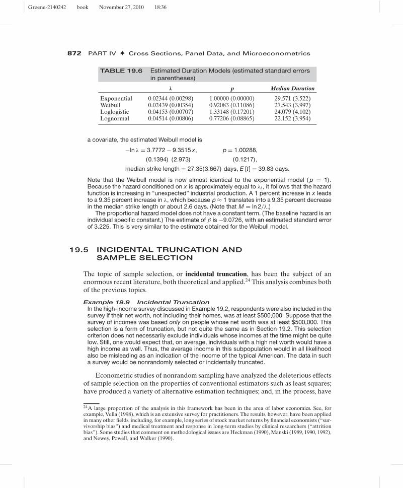
Greene-2140242 book November 27, 2010 18:36
872 PART IV ✦ Cross Sections, Panel Data, and Microeconometrics
TABLE 19.6 Estimated Duration Models (estimated standard errorsin parentheses)
λ p Median Duration
Exponential 0.02344 (0.00298) 1.00000 (0.00000) 29.571 (3.522)Weibull 0.02439 (0.00354) 0.92083 (0.11086) 27.543 (3.997)Loglogistic 0.04153 (0.00707) 1.33148 (0.17201) 24.079 (4.102)Lognormal 0.04514 (0.00806) 0.77206 (0.08865) 22.152 (3.954)
a covariate, the estimated Weibull model is
−ln λ = 3.7772 − 9.3515 x, p = 1.00288,
(0.1394) (2.973) (0.1217) ,
median strike length = 27.35(3.667) days, E [t] = 39.83 days.
Note that the Weibull model is now almost identical to the exponential model ( p = 1) .Because the hazard conditioned on x is approximately equal to λi , it follows that the hazardfunction is increasing in “unexpected” industrial production. A 1 percent increase in x leadsto a 9.35 percent increase in λ, which because p ≈ 1 translates into a 9.35 percent decreasein the median strike length or about 2.6 days. (Note that M = ln 2/λ.)
The proportional hazard model does not have a constant term. (The baseline hazard is anindividual specific constant.) The estimate of β is −9.0726, with an estimated standard errorof 3.225. This is very similar to the estimate obtained for the Weibull model.
19.5 INCIDENTAL TRUNCATION ANDSAMPLE SELECTION
The topic of sample selection, or incidental truncation, has been the subject of anenormous recent literature, both theoretical and applied.24 This analysis combines bothof the previous topics.
Example 19.9 Incidental TruncationIn the high-income survey discussed in Example 19.2, respondents were also included in thesurvey if their net worth, not including their homes, was at least $500,000. Suppose that thesurvey of incomes was based only on people whose net worth was at least $500,000. Thisselection is a form of truncation, but not quite the same as in Section 19.2. This selectioncriterion does not necessarily exclude individuals whose incomes at the time might be quitelow. Still, one would expect that, on average, individuals with a high net worth would have ahigh income as well. Thus, the average income in this subpopulation would in all likelihoodalso be misleading as an indication of the income of the typical American. The data in sucha survey would be nonrandomly selected or incidentally truncated.
Econometric studies of nonrandom sampling have analyzed the deleterious effectsof sample selection on the properties of conventional estimators such as least squares;have produced a variety of alternative estimation techniques; and, in the process, have
24A large proportion of the analysis in this framework has been in the area of labor economics. See, forexample, Vella (1998), which is an extensive survey for practitioners. The results, however, have been appliedin many other fields, including, for example, long series of stock market returns by financial economists (“sur-vivorship bias”) and medical treatment and response in long-term studies by clinical researchers (“attritionbias”). Some studies that comment on methodological issues are Heckman (1990), Manski (1989, 1990, 1992),and Newey, Powell, and Walker (1990).
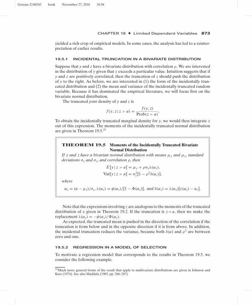
Greene-2140242 book November 27, 2010 18:36
CHAPTER 19 ✦ Limited Dependent Variables 873
yielded a rich crop of empirical models. In some cases, the analysis has led to a reinter-pretation of earlier results.
19.5.1 INCIDENTAL TRUNCATION IN A BIVARIATE DISTRIBUTION
Suppose that y and z have a bivariate distribution with correlation ρ. We are interestedin the distribution of y given that z exceeds a particular value. Intuition suggests that ify and z are positively correlated, then the truncation of z should push the distributionof y to the right. As before, we are interested in (1) the form of the incidentally trun-cated distribution and (2) the mean and variance of the incidentally truncated randomvariable. Because it has dominated the empirical literature, we will focus first on thebivariate normal distribution.
The truncated joint density of y and z is
f (y, z | z > a) = f (y, z)Prob(z > a)
.
To obtain the incidentally truncated marginal density for y, we would then integrate zout of this expression. The moments of the incidentally truncated normal distributionare given in Theorem 19.5.25
THEOREM 19.5 Moments of the Incidentally Truncated BivariateNormal Distribution
If y and z have a bivariate normal distribution with means μy and μz, standarddeviations σy and σz, and correlation ρ, then
E [y | z > a] = μy + ρσyλ(αz),
Var[y | z > a] = σ 2y [1 − ρ2δ(αz)],
where
αz = (a − μz)/σz, λ(αz) = φ(αz)/[1 − �(αz)], and δ(αz) = λ(αz)[λ(αz) − αz].
Note that the expressions involving z are analogous to the moments of the truncateddistribution of x given in Theorem 19.2. If the truncation is z< a, then we make thereplacement λ(αz) = −φ(αz)/�(αz).
As expected, the truncated mean is pushed in the direction of the correlation if thetruncation is from below and in the opposite direction if it is from above. In addition,the incidental truncation reduces the variance, because both δ(α) and ρ2 are betweenzero and one.
19.5.2 REGRESSION IN A MODEL OF SELECTION
To motivate a regression model that corresponds to the results in Theorem 19.5, weconsider the following example.
25Much more general forms of the result that apply to multivariate distributions are given in Johnson andKotz (1974). See also Maddala (1983, pp. 266–267).

Greene-2140242 book November 27, 2010 18:36
874 PART IV ✦ Cross Sections, Panel Data, and Microeconometrics
Example 19.10 A Model of Labor SupplyA simple model of female labor supply that has been examined in many studies consists oftwo equations:26
1. Wage equation. The difference between a person’s market wage, what she could com-mand in the labor market, and her reservation wage, the wage rate necessary to makeher choose to participate in the labor market, is a function of characteristics such as ageand education as well as, for example, number of children and where a person lives.
2. Hours equation. The desired number of labor hours supplied depends on the wage, homecharacteristics such as whether there are small children present, marital status, and soon.
The problem of truncation surfaces when we consider that the second equation describesdesired hours, but an actual figure is observed only if the individual is working. (In mostsuch studies, only a participation equation, that is, whether hours are positive or zero, isobservable.) We infer from this that the market wage exceeds the reservation wage. Thus,the hours variable in the second equation is incidentally truncated.
To put the preceding examples in a general framework, let the equation that deter-mines the sample selection be
z∗i = w′
iγ + ui ,
and let the equation of primary interest be
yi = x′iβ + εi .
The sample rule is that yi is observed only when z∗i is greater than zero. Suppose as
well that εi and ui have a bivariate normal distribution with zero means and correlationρ. Then we may insert these in Theorem 19.5 to obtain the model that applies to theobservations in our sample:
E [yi | yi is observed] = E [yi | z∗i > 0]
= E [yi | ui > −w′iγ ]
= x′iβ + E [εi | ui > −w′
iγ ]
= x′iβ + ρσελi (αu)
= x′iβ + βλλi (αu),
where αu = −w′iγ /σu and λ(αu) = φ(w′
iγ /σu)/�(w′iγ /σu). So,
yi | z∗i > 0 = E [yi | z∗
i > 0] + vi
= x′iβ + βλλi (αu) + vi .
Least squares regression using the observed data—for instance, OLS regression of hourson its determinants, using only data for women who are working—produces inconsistentestimates of β. Once again, we can view the problem as an omitted variable. Leastsquares regression of y on x and λ would be a consistent estimator, but if λ is omitted,then the specification error of an omitted variable is committed. Finally, note that thesecond part of Theorem 19.5 implies that even if λi were observed, then least squareswould be inefficient. The disturbance vi is heteroscedastic.
26See, for example, Heckman (1976). This strand of literature begins with an exchange by Gronau (1974) andLewis (1974).
Greene-2140242 book November 27, 2010 18:36
CHAPTER 19 ✦ Limited Dependent Variables 875
The marginal effect of the regressors on yi in the observed sample consists of twocomponents. There is the direct effect on the mean of yi , which is β. In addition, for aparticular independent variable, if it appears in the probability that z∗
i is positive, thenit will influence yi through its presence in λi . The full effect of changes in a regressorthat appears in both xi and wi on y is
∂ E [yi | z∗i > 0]
∂xik= βk − γk
(ρσε
σu
)δi (αu),
where27
δi = λ2i − αiλi .
Suppose that ρ is positive and E [yi ] is greater when z∗i is positive than when it is negative.
Because 0 < δi < 1, the additional term serves to reduce the marginal effect. The changein the probability affects the mean of yi in that the mean in the group z∗
i > 0 is higher.The second term in the derivative compensates for this effect, leaving only the marginaleffect of a change given that z∗
i > 0 to begin with. Consider Example 19.12, and supposethat education affects both the probability of migration and the income in either state.If we suppose that the income of migrants is higher than that of otherwise identicalpeople who do not migrate, then the marginal effect of education has two parts, onedue to its influence in increasing the probability of the individual’s entering a higher-income group and one due to its influence on income within the group. As such, thecoefficient on education in the regression overstates the marginal effect of the educationof migrants and understates it for nonmigrants. The sizes of the various parts dependon the setting. It is quite possible that the magnitude, sign, and statistical significance ofthe effect might all be different from those of the estimate of β, a point that appearsfrequently to be overlooked in empirical studies.
In most cases, the selection variable z∗ is not observed. Rather, we observe onlyits sign. To consider our two examples, we typically observe only whether a woman isworking or not working or whether an individual migrated or not. We can infer the signof z∗, but not its magnitude, from such information. Because there is no information onthe scale of z∗, the disturbance variance in the selection equation cannot be estimated.(We encountered this problem in Chapter 17 in connection with the probit model.)Thus, we reformulate the model as follows:
selection mechanism: z∗i = w′
iγ + ui , zi = 1 if z∗i > 0 and 0 otherwise;
Prob(zi = 1 | wi ) = �(w′iγ ); and
Prob(zi = 0 | wi ) = 1 − �(w′iγ ).
regression model: yi = x′iβ + εi observed only if zi = 1,
(ui , εi ) ∼ bivariate normal [0, 0, 1, σε, ρ].
(19-22)
Suppose that, as in many of these studies, zi and wi are observed for a random sampleof individuals but yi is observed only when zi = 1. This model is precisely the one we
27We have reversed the sign of αu in (Theorem 19.5) because a = 0, and α = w′γ /σM is somewhat moreconvenient. Also, as such, ∂λ/∂α = −δ.

Greene-2140242 book November 27, 2010 18:36
876 PART IV ✦ Cross Sections, Panel Data, and Microeconometrics
examined earlier, with
E [yi | zi = 1, xi , wi ] = x′iβ + ρσελ(w′
iγ ).
19.5.3 TWO-STEP AND MAXIMUM LIKELIHOOD ESTIMATION
The parameters of the sample selection model can be estimated by maximum like-lihood.28 However, Heckman’s (1979) two-step estimation procedure is usually usedinstead. Heckman’s method is as follows:29
1. Estimate the probit equation by maximum likelihood to obtain estimates of γ .For each observation in the selected sample, compute λi = φ(w′
i γ )/�(w′i γ ) and
δi = λi (λi + w′i γ ).
2. Estimate β and βλ = ρσε by least squares regression of y on x and λ.
It is possible also to construct consistent estimators of the individual parameters ρ
and σε. At each observation, the true conditional variance of the disturbance would be
σ 2i = σ 2
ε (1 − ρ2δi ).
The average conditional variance for the sample would converge to
plim1n
n∑i=1
σ 2i = σ 2
ε (1 − ρ2δ),
which is what is estimated by the least squares residual variance e′e/n. For the squareof the coefficient on λ, we have
plim b2λ = ρ2σ 2
ε ,
whereas based on the probit results we have
plim1n
n∑i=1
δi = δ.
We can then obtain a consistent estimator of σ 2ε using
σ 2ε = 1
ne′e + ˆδb2
λ.
Finally, an estimator of ρ2 is
ρ2 = b2λ
σ 2ε
, (19-23)
which provides a complete set of estimators of the model’s parameters.30
To test hypotheses, an estimate of the asymptotic covariance matrix of [b′, bλ] isneeded. We have two problems to contend with. First, we can see in Theorem 19.5 that
28See Greene (1995a).29Perhaps in a mimicry of the “tobit” estimator described earlier, this procedure has come to be known asthe “Heckit” estimator.30Note that ρ2 is not a sample correlation and, as such, is not limited to [0, 1]. See Greene (1981) for discussion.

Greene-2140242 book November 27, 2010 18:36
CHAPTER 19 ✦ Limited Dependent Variables 877
the disturbance term in
(yi | zi = 1, xi , wi ) = x′iβ + ρσελi + vi (19-24)
is heteroscedastic;
Var[vi | zi = 1, xi , wi ] = σ 2ε (1 − ρ2δi ).
Second, there are unknown parameters in λi . Suppose that we assume for the momentthat λi and δi are known (i.e., we do not have to estimate γ ). For convenience, letx∗
i = [xi , λi ], and let b∗ be the least squares coefficient vector in the regression of y onx∗ in the selected data. Then, using the appropriate form of the variance of ordinaryleast squares in a heteroscedastic model from Chapter 9, we would have to estimate
Var[b∗] = σ 2ε [X′
∗X∗]−1
[n∑
i=1
(1 − ρ2δi )x∗i x∗′
i
][X′
∗X∗]−1
= σ 2ε [X′
∗X∗]−1[X′∗(I − ρ2 )X∗][X′
∗X∗]−1,
where I − ρ2 is a diagonal matrix with (1 − ρ2δi ) on the diagonal. Without any othercomplications, this result could be computed fairly easily using X, the sample estimatesof σ 2
ε and ρ2, and the assumed known values of λi and δi .The parameters in γ do have to be estimated using the probit equation. Rewrite
(19-24) as
(yi | zi = 1, xi , wi ) = x′iβ + βλλi + vi − βλ(λi − λi ).
In this form, we see that in the preceding expression we have ignored both an additionalsource of variation in the compound disturbance and correlation across observations;the same estimate of γ is used to compute λi for every observation. Heckman hasshown that the earlier covariance matrix can be appropriately corrected by adding aterm inside the brackets,
Q = ρ2(X′∗ W)Est. Asy. Var[γ ](W′ X∗) = ρ2FVF ′,
where V = Est. Asy. Var[γ ], the estimator of the asymptotic covariance of the probitcoefficients. Any of the estimators in (17-22) to (17-24) may be used to compute V. Thecomplete expression is31
Est. Asy. Var[b, bλ] = σ 2ε [X′
∗X∗]−1[X′∗(I − ρ2 )X∗ + Q][X′
∗X∗]−1.
The sample selection model can also be estimated by maximum likelihood. The fulllog-likelihood function for the data is built up from
Prob(selection) × density | selection for observations with zi = 1,
and
Prob(nonselection) for observations with zi = 0.
31This matrix formulation is derived in Greene (1981). Note that the Murphy and Topel (1985) results fortwo-step estimators given in Theorem 14.8 would apply here as well. Asymptotically, this method would givethe same answer. The Heckman formulation has become standard in the literature.

Greene-2140242 book November 27, 2010 18:36
878 PART IV ✦ Cross Sections, Panel Data, and Microeconometrics
Combining the parts produces the full log-likelihood function,
ln L =∑z=1
ln
[exp
(−(1/2)ε2i /σ
2ε
)σε
√2π
�
(ρεi/σε + w′
iγ√1 − ρ2
)]+
∑z=0
[1 − ln �(w′iγ )],
where εi = yi −x′iβ. Note, the FIML estimator with its assumption of bivariate normality
is not less robust than the two-step estimator. because the latter also requires bivariatenormality to form the conditional mean for the regression.
Two virtues of the FIML estimator will be the greater efficiency brought by usingthe likelihood function rather than the method of moments and, second, the estimationof ρ subject to the constraint −1 < ρ < 1. (This is typically done by reparameterizingthe model in terms of the monotonic inverse hyperbolic tangent, τ = (1/2) ln [(1 +ρ)/(1 − ρ)] = atanh(ρ). The transformed parameter, τ , is unrestricted. The inversetransformation is ρ = [exp(2τ) − 1]/[exp(2τ) + 1] which is bounded between zeroand one.) One possible drawback (it might be argued) could be the complexity ofthe likelihood function that would make estimation more difficult than the two-stepestimator. However, the MLE for the selection model appears as a built-in procedurein modern software such as Stata and NLOGIT, and it is straightforward to implementin Gauss and MatLab, so this might be a moot point. Surprisingly, the MLE is by far lesscommon than the two-step estimator in the received applications. The estimation of ρ
is the difficult part of the estimaton process (this is often the case). It is quite commonfor the method of moments estimator and the FIML estimator to be very different—our application in Example 19.11 is a case. Perhaps surprisingly so, the moment-basedestimator of ρ in (19-23) is not bounded by zero and one. [See Greene (1981).] Thiswould seem to recommend the MLE.
The fully parametric bivariate normality assumption of the model has been viewedas a potential drawback. However, relatively little progress has been made on devisinginformative semi- and nonparametric estimators—see, for one example, Gallant andNychka (1987). The obstacle here is that, ultimately, the model hangs on a parame-terization of the correlation of the unobservables in the two equations. So, method ofmoment estimators or kernel-based estimators must still incorporate this feature of abivariate distribution. Some results have been obtained using the method of copulafunctions. [See Smith (2003, 2005) and Trivedi and Zimmer (2007).]
Example 19.11 Female Labor SupplyExamples 17.1 and 17.8 proposed a labor force participation model for a sample of 753married women in a sample analyzed by Mroz (1987). The data set contains wage and hoursinformation for the 428 women who participated in the formal market (LFP=1). FollowingMroz, we suppose that for these 428 individuals, the offered wage exceeded the reservationwage and, moreover, the unobserved effects in the two wage equations are correlated. Assuch, a wage equation based on the market data should account for the sample selectionproblem. We specify a simple wage model:
Wage = β1 + β2 Exper + β3 Exper 2 + β4 Education + β5 City + ε
where Exper is labor market experience and City is a dummy variable indicating that theindividual lived in a large urban area. Maximum likelihood, Heckman two-step, and ordinaryleast squares estimates of the wage equation are shown in Table 19.7. The maximum likeli-hood estimates are FIML estimates—the labor force participation equation is reestimated atthe same time. Only the parameters of the wage equation are shown next. Note as well thatthe two-step estimator estimates the single coefficient on λi and the structural parameters σ
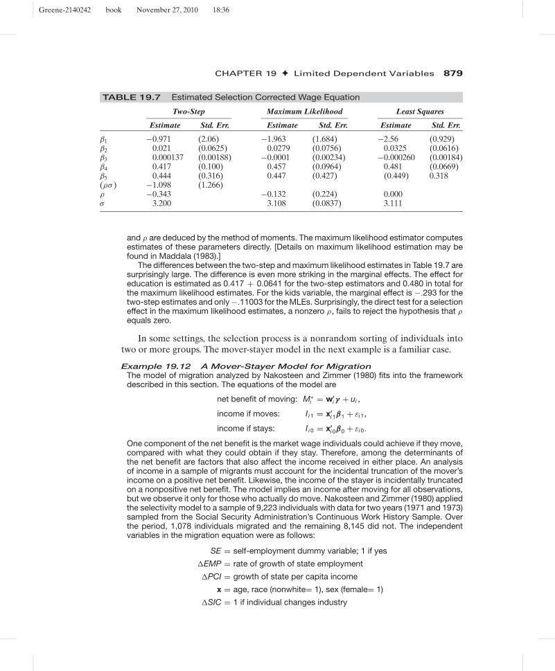
Greene-2140242 book November 27, 2010 18:36
CHAPTER 19 ✦ Limited Dependent Variables 879
TABLE 19.7 Estimated Selection Corrected Wage Equation
Two-Step Maximum Likelihood Least Squares
Estimate Std. Err. Estimate Std. Err. Estimate Std. Err.
β1 −0.971 (2.06) −1.963 (1.684) −2.56 (0.929)β2 0.021 (0.0625) 0.0279 (0.0756) 0.0325 (0.0616)β3 0.000137 (0.00188) −0.0001 (0.00234) −0.000260 (0.00184)β4 0.417 (0.100) 0.457 (0.0964) 0.481 (0.0669)β5 0.444 (0.316) 0.447 (0.427) (0.449) 0.318(ρσ ) −1.098 (1.266)ρ −0.343 −0.132 (0.224) 0.000σ 3.200 3.108 (0.0837) 3.111
and ρ are deduced by the method of moments. The maximum likelihood estimator computesestimates of these parameters directly. [Details on maximum likelihood estimation may befound in Maddala (1983).]
The differences between the two-step and maximum likelihood estimates in Table 19.7 aresurprisingly large. The difference is even more striking in the marginal effects. The effect foreducation is estimated as 0.417 + 0.0641 for the two-step estimators and 0.480 in total forthe maximum likelihood estimates. For the kids variable, the marginal effect is −.293 for thetwo-step estimates and only −.11003 for the MLEs. Surprisingly, the direct test for a selectioneffect in the maximum likelihood estimates, a nonzero ρ, fails to reject the hypothesis that ρequals zero.
In some settings, the selection process is a nonrandom sorting of individuals intotwo or more groups. The mover-stayer model in the next example is a familiar case.
Example 19.12 A Mover-Stayer Model for MigrationThe model of migration analyzed by Nakosteen and Zimmer (1980) fits into the frameworkdescribed in this section. The equations of the model are
net benefit of moving: M∗i = w′
i γ + ui ,
income if moves: I i 1 = x′i 1β1 + εi 1,
income if stays: I i 0 = x′i 0β0 + εi 0.
One component of the net benefit is the market wage individuals could achieve if they move,compared with what they could obtain if they stay. Therefore, among the determinants ofthe net benefit are factors that also affect the income received in either place. An analysisof income in a sample of migrants must account for the incidental truncation of the mover’sincome on a positive net benefit. Likewise, the income of the stayer is incidentally truncatedon a nonpositive net benefit. The model implies an income after moving for all observations,but we observe it only for those who actually do move. Nakosteen and Zimmer (1980) appliedthe selectivity model to a sample of 9,223 individuals with data for two years (1971 and 1973)sampled from the Social Security Administration’s Continuous Work History Sample. Overthe period, 1,078 individuals migrated and the remaining 8,145 did not. The independentvariables in the migration equation were as follows:
SE = self-employment dummy variable; 1 if yes
�EMP = rate of growth of state employment
�PCI = growth of state per capita income
x = age, race (nonwhite= 1), sex (female= 1)
�SIC = 1 if individual changes industry
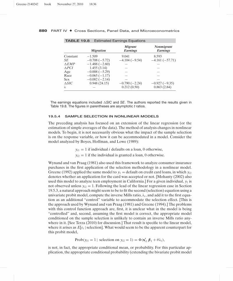
Greene-2140242 book November 27, 2010 18:36
880 PART IV ✦ Cross Sections, Panel Data, and Microeconometrics
TABLE 19.8 Estimated Earnings Equations
Migrant NonmigrantMigration Earnings Earnings
Constant −1.509 9.041 8.593SE −0.708 (−5.72) −4.104 (−9.54) −4.161 (−57.71)�EMP −1.488 (−2.60) — —�PCI 1.455 (3.14) — —Age −0.008 (−5.29) — —Race −0.065 (−1.17) — —Sex −0.082 (−2.14) — —�SIC 0.948 (24.15) −0.790 (−2.24) −0.927 (−9.35)λ — 0.212 (0.50) 0.863 (2.84)
The earnings equations included �SIC and SE. The authors reported the results given inTable 19.8. The figures in parentheses are asymptotic t ratios.
19.5.4 SAMPLE SELECTION IN NONLINEAR MODELS
The preceding analysis has focused on an extension of the linear regression (or theestimation of simple averages of the data). The method of analysis changes in nonlinearmodels. To begin, it is not necessarily obvious what the impact of the sample selectionis on the response variable, or how it can be accommodated in a model. Consider themodel analyzed by Boyes, Hoffman, and Lowe (1989):
yi1 = 1 if individual i defaults on a loan, 0 otherwise,
yi2 = 1 if the individual is granted a loan, 0 otherwise.
Wynand and van Praag (1981) also used this framework to analyze consumer insurancepurchases in the first application of the selection methodology in a nonlinear model.Greene (1992) applied the same model to y1 = default on credit card loans, in which yi2
denotes whether an application for the card was accepted or not. [Mohanty (2002) alsoused this model to analyze teen employment in California.] For a given individual, y1 isnot observed unless yi2 = 1. Following the lead of the linear regression case in Section19.5.3, a natural approach might seem to be to fit the second (selection) equation using aunivariate probit model, compute the inverse Mills ratio, λi , and add it to the first equa-tion as an additional “control” variable to accommodate the selection effect. [This isthe approach used by Wynand and van Praag (1981) and Greene (1994).] The problemswith this control function approach are, first, it is unclear what in the model is being“controlled” and, second, assuming the first model is correct, the appropriate modelconditioned on the sample selection is unlikely to contain an inverse Mills ratio any-where in it. [See Terza (2010) for discussion.] That result is specific to the linear model,where it arises as E[εi | selection]. What would seem to be the apparent counterpart forthis probit model,
Prob(yi1 = 1 | selection on yi2 = 1) = �(x′i1 β1 + θλi ),
is not, in fact, the appropriate conditional mean, or probability. For this particular ap-plication, the appropriate conditional probability (extending the bivariate probit model

Greene-2140242 book November 27, 2010 18:36
CHAPTER 19 ✦ Limited Dependent Variables 881
of Section 17.5) would be
Prob[yi1 = 1 | yi2 = 1] = �2(x′i1β1, x′
i2β2, ρ)
�(x′i2β2)
.
We would use this result to build up the likelihood function for the three observed out-comes, as follows: The three types of observations in the sample, with their unconditionalprobabilities, are
yi2 = 0: Prob(yi2 = 0 | xi1, xi2) = 1 − �(x′i2β2),
yi1 = 0, yi2 = 1: Prob(yi1 = 0, yi2 = 1| xi1, xi2) = �2(−x′i1β1, x′
i2β2, −ρ),
yi1 = 1, yi2 = 1: Prob(yi1 = 1, yi2 = 1| xi1, xi2) = �2(x′i1β1, x′
i2β2, ρ).
(19-25)
The log-likelihood function is based on these probabilities.32 An application appears inSection 17.5.6.
Example 19.13 Doctor Visits and InsuranceContinuing our analysis of the utilization of the German health care system, we observe thatthe data set contains an indicator of whether the individual subscribes to the “Public” healthinsurance or not. Roughly 87 percent of the observations in the sample do. We might askwhether the selection on public insurance reveals any substantive difference in visits to thephysician. We estimated a logit specification for this model in Example 17.4. Using (19-25)as the framework, we define yi 2 to be presence of insurance and yi 1 to be the binary variabledefined to equal 1 if the individual makes at least one visit to the doctor in the survey year.
The estimation results are given in Table 19.9. Based on these results, there does appearto be a very strong relationship. The coefficients do change somewhat in the conditionalmodel. A Wald test for the presence of the selection effect against the null hypothesis that ρequals zero produces a test statistic of (−7.188)2 = 51.667, which is larger than the criticalvalue of 3.84. Thus, the hypothesis is rejected. A likelihood ratio statistic is computed asthe difference between the log-likelihood for the full model and the sum of the two separatelog-likelihoods for the independent probit models when ρ equals zero. The result is
λLR = 2[−23969.58 − (−15536.39 + (−8471.508) ) = 77.796
The hypothesis is rejected once again. Partial effects were computed using the results inSection 17.5.3.
The large correlation coefficient can be misleading. The estimated −0.9299 does notstate that the presence of insurance makes it much less likely to go to the doctor. This isthe correlation among the unobserved factors in each equation. The factors that make itmore likely to purchase insurance make it less likely to use a physician. To obtain a simplecorrelation between the two variables, we might use the tetrachoric correlation defined inExample 17.18. This would be computed by fitting a bivariate probit model for the two binaryvariables without any other variables. The estimated value is 0.120.
More general cases are typically much less straightforward. Greene (2005, 2006,2010) and Terza (1998, 2010) present sample selection models for nonlinear specifica-tions based on the underlying logic of the Heckman model in Section 19.5.3, that theinfluence of the incidental truncation acts on the unobservable variables in the model.(That is the source of the “selection bias” in conventional estimators.) The modelingextension introduces the unobservables into the model in a natural fashion that parallelsthe regression model. Terza (2010) presents a survey of the general results.
32Extensions of the bivariate probit model to other types of censoring are discussed in Poirier (1980) andAbowd and Farber (1982).
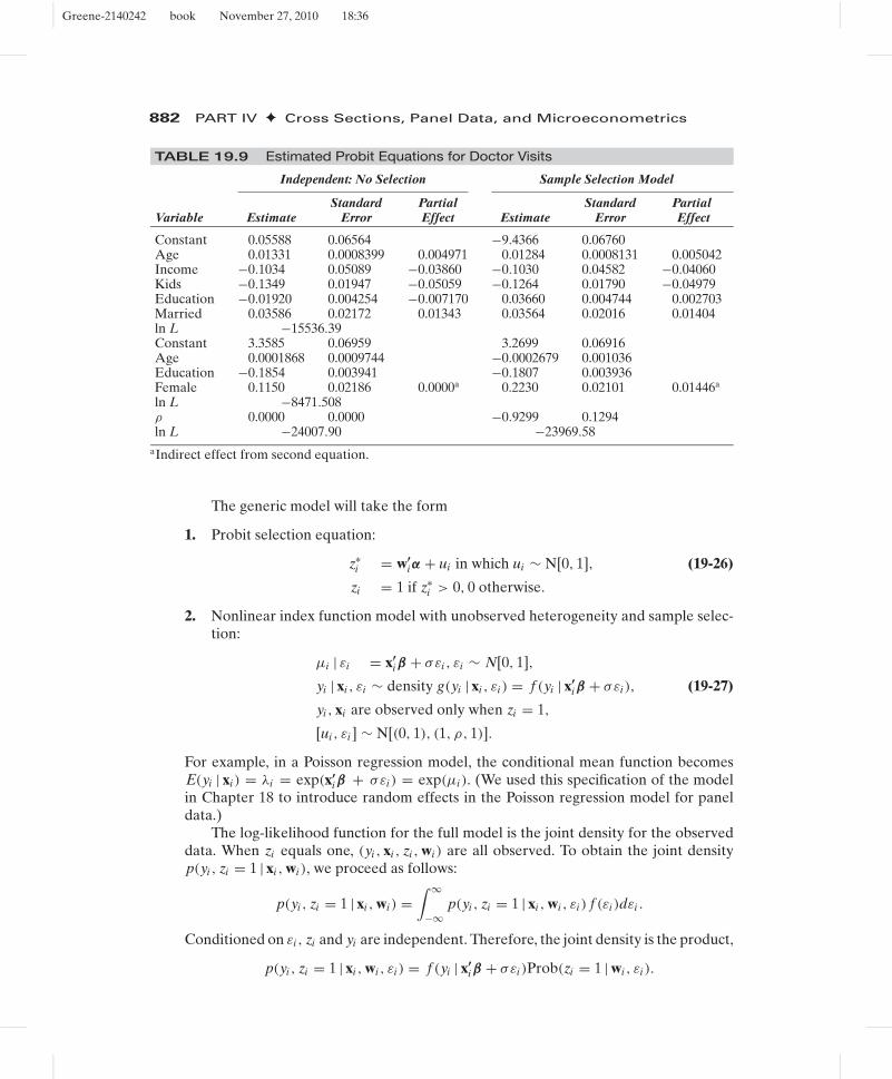
Greene-2140242 book November 27, 2010 18:36
882 PART IV ✦ Cross Sections, Panel Data, and Microeconometrics
TABLE 19.9 Estimated Probit Equations for Doctor Visits
Independent: No Selection Sample Selection Model
Standard Partial Standard PartialVariable Estimate Error Effect Estimate Error Effect
Constant 0.05588 0.06564 −9.4366 0.06760Age 0.01331 0.0008399 0.004971 0.01284 0.0008131 0.005042Income −0.1034 0.05089 −0.03860 −0.1030 0.04582 −0.04060Kids −0.1349 0.01947 −0.05059 −0.1264 0.01790 −0.04979Education −0.01920 0.004254 −0.007170 0.03660 0.004744 0.002703Married 0.03586 0.02172 0.01343 0.03564 0.02016 0.01404ln L −15536.39Constant 3.3585 0.06959 3.2699 0.06916Age 0.0001868 0.0009744 −0.0002679 0.001036Education −0.1854 0.003941 −0.1807 0.003936Female 0.1150 0.02186 0.0000a 0.2230 0.02101 0.01446a
ln L −8471.508ρ 0.0000 0.0000 −0.9299 0.1294ln L −24007.90 −23969.58
aIndirect effect from second equation.
The generic model will take the form
1. Probit selection equation:
z∗i = w′
iα + ui in which ui ∼ N[0, 1], (19-26)
zi = 1 if z∗i > 0, 0 otherwise.
2. Nonlinear index function model with unobserved heterogeneity and sample selec-tion:
μi | εi = x′iβ + σεi , εi ∼ N[0, 1],
yi | xi , εi ∼ density g(yi | xi , εi ) = f (yi | x′iβ + σεi ), (19-27)
yi , xi are observed only when zi = 1,
[ui , εi ] ∼ N[(0, 1), (1, ρ, 1)].
For example, in a Poisson regression model, the conditional mean function becomesE(yi | xi ) = λi = exp(x′
iβ + σεi ) = exp(μi ). (We used this specification of the modelin Chapter 18 to introduce random effects in the Poisson regression model for paneldata.)
The log-likelihood function for the full model is the joint density for the observeddata. When zi equals one, (yi , xi , zi , wi ) are all observed. To obtain the joint densityp(yi , zi = 1 | xi , wi ), we proceed as follows:
p(yi , zi = 1 | xi , wi ) =∫ ∞
−∞p(yi , zi = 1 | xi , wi , εi ) f (εi )dεi .
Conditioned on εi , zi and yi are independent. Therefore, the joint density is the product,
p(yi , zi = 1 | xi , wi , εi ) = f (yi | x′iβ + σεi )Prob(zi = 1 | wi , εi ).

Greene-2140242 book November 27, 2010 18:36
CHAPTER 19 ✦ Limited Dependent Variables 883
The first part, f (yi | x′iβ + σεi ) is the conditional index function model in (19-27). By
joint normality, f (ui | εi ) = N[ρεi , (1 − ρ2)], so ui | εi = ρεi + (ui − ρεi ) = ρεi + vi
where E[vi ] = 0 and Var[vi ] = (1 − ρ2). Therefore,
Prob(zi = 1 | wi , εi ) = �
(w′
iα + ρεi√1 − ρ2
).
Combining terms and using the earlier approach, the unconditional joint density is
p(yi , zi = 1 | xi , wi ) =∫ ∞
−∞f (yi | x′
iβ + σεi )�
(w′
iα + ρεi√1 − ρ2
)exp
(−ε2i
/2)
√2π
dεi . (19-28)
The other part of the likelihood function for the observations with zi = 0 will be
Prob(zi = 0 | wi ) =∫ ∞
−∞Prob(zi = 0 | wi , εi ) f (εi )dεi .
=∫ ∞
−∞
[1 − �
(w′
iα + ρεi√1 − ρ2
)]f (εi )dεi (19-29)
=∫ ∞
−∞�
(−(w′
iα + ρεi )√1 − ρ2
)exp
(−ε2i
/2)
√2π
dεi .
For convenience, we can use the invariance principle to reparameterize the likelihoodfunction in terms of γ = α/
√1 − ρ2 and τ = ρ/
√1 − ρ2. Combining all the preceding
terms, the log-likelihood function to be maximized is
ln L =n∑
i=1
ln∫ ∞
−∞[(1−zi )+zi f (yi | x′
iβ+σεi )]�[(2zi −1)(w′iγ +τεi )]φ(εi )dεi . (19-30)
This can be maximized with respect to (β, σ, γ , τ ) using quadrature or simulation. Whendone, ρ can be recovered from ρ = τ /(1 + τ 2)1/2 and α = (1 − ρ2)1/2γ . All that differsfrom one model to another is the specification of f (yi | x′
iβ+σεi ). This is the specificationused in Terza (1998) and Terza and Kenkel (2001). (In these two papers, the authorsalso analyzed E[yi | zi = 1]. This estimator was based on nonlinear least squares, but asearlier, it is necessary to integrate the unobserved heterogeneity out of the conditionalmean function.) Greene (2010) applies the method to a stochastic frontier model.
19.5.5 PANEL DATA APPLICATIONS OF SAMPLESELECTION MODELS
The development of methods for extending sample selection models to panel datasettings parallels the literature on cross-section methods. It begins with Hausman andWise (1979) who devised a maximum likelihood estimator for a two-period model withattrition—the “selection equation” was a formal model for attrition from the sample.Subsequent research has drawn the analogy between attrition and sample selection ina variety of applications, such as Keane et al. (1988) and Verbeek and Nijman (1992),and produced theoretical developments including Wooldridge (2002a, b).
The direct extension of panel data methods to sample selection brings several newissues for the modeler. An immediate question arises concerning the nature of the

Greene-2140242 book November 27, 2010 18:36
884 PART IV ✦ Cross Sections, Panel Data, and Microeconometrics
selection itself. Although much of the theoretical literature [e.g., Kyriazidou (1997,2001)] treats the panel as if the selection mechanism is run anew in every period, inpractice, the selection process often comes in two very different forms. First, selectionmay take the form of selection of the entire group of observations into the panel dataset. Thus, the selection mechanism operates once, perhaps even before the observationwindow opens. Consider the entry (or not) of eligible candidates for a job trainingprogram. In this case, it is not appropriate to build the model to allow entry, exit, andthen reentry. Second, for most applications, selection comes in the form of attrition orretention. Once an observation is “deselected,” it does not return. Leading exampleswould include “survivorship” in time-series–cross-section models of firm performanceand attrition in medical trials and in panel data applications involving large nationalsurvey data bases, such as Contoyannis et al. (2004). Each of these cases suggests theutility of a more structured approach to the selection mechanism.
19.5.5.a Common Effects in Sample Selection Models
A formal “effects” treatment for sample selection was first suggested in complete formby Verbeek (1990), who formulated a random effects model for the probit equation anda fixed effects approach for the main regression. Zabel (1992) criticized the specificationfor its asymmetry in the treatment of the effects in the two equations. He also argued thatthe likelihood function that neglected correlation between the effects and regressors inthe probit model would render the FIML estimator inconsistent. His proposal involvedfixed effects in both equations. Recognizing the difficulty of fitting such a model, hethen proposed using the Mundlak correction. The full model is
y∗it = ηi + x′
itβ + εit, ηi = x′iπ + τwi , wi ∼ N[0, 1],
d∗it = θi + z′
itα + uit, θi = z′iδ + ωvi , vi ∼ N[0, 1], (19-31)
(εit, uit) ∼ N2[(0, 0), (σ 2, 1, ρσ )].
The “selectivity” in the model is carried through the correlation between εit and uit. Theresulting log-likelihood is built up from the contribution of individual i ,
Li =∫ ∞
−∞
∏dit=0
�[−z′itα − z′
iδ − ωvi ]φ(vi )dvi
×∫ ∞
−∞
∫ ∞
−∞
∏dit=1
�
[z′
itα + z′iδ + ωvi + (ρ/σ)εit√
1 − ρ2
]
× 1σ
φ(εit
σ
)φ2(vi , wi )dvi dwi , (19-32)
εit = yit − x′itβ − x′
iπ − τwi .
The log-likelihood is then ln L = ∑i ln Li .
The log-likelihood requires integration in two dimensions for any selected obser-vations. Vella (1998) suggested two-step procedures to avoid the integration. However,the bivariate normal integration is actually the product of two univariate normals, be-cause in the preceding specification, vi and wi are assumed to be uncorrelated. As such,the likelihood function in (19-32) can be readily evaluated using familiar simulationor quadrature techniques. [See Sections 14.9.6.c and 15.6. Vella and Verbeek (1999)

Greene-2140242 book November 27, 2010 18:36
CHAPTER 19 ✦ Limited Dependent Variables 885
suggest this in a footnote, but do not pursue it.] To show this, note that the first linein the log-likelihood is of the form Ev[
∏d=0 �(. . .)] and the second line is of the form
Ew[Ev[�(. . .)φ(. . .)/σ ]]. Either of these expectations can be satisfactorily approximatedwith the average of a sufficient number of draws from the standard normal populationsthat generate wi and vi . The term in the simulated likelihood that follows this prescrip-tion is
LSi = 1
R
R∑r=1
∏dit=0
�[−z′itα − z′
iδ − ωvi,r ]
× 1R
R∑r=1
∏dit=1
�
[z′
itα + z′iδ + ωvi,r + (ρ/σ)εit,r√
1 − ρ2
]1σ
φ(εit,r
σ
), (19-33)
εit,r = yit − x′itβ − x′
iπ − τwi,r .
Maximization of this log-likelihood with respect to (β,σ,ρ,α,δ,π ,τ,ω) by conventionalgradient methods is quite feasible. Indeed, this formulation provides a means by whichthe likely correlation between vi and wi can be accommodated in the model. Supposethat wi and vi are bivariate standard normal with correlation ρvw . We can project wi onvi and write
wi = ρvwvi + (1 − ρ2
vw
)1/2hi ,
where hi has a standard normal distribution. To allow the correlation, we now simplysubstitute this expression for wi in the simulated (or original) log-likelihood and addρvw to the list of parameters to be estimated. The simulation is still over independentnormal variates, vi and hi .
Notwithstanding the preceding derivation, much of the recent attention has focusedon simpler two-step estimators. Building on Ridder and Wansbeek (1990) and Verbeekand Nijman (1992) [see Vella (1998) for numerous additional references], Vella andVerbeek (1999) purpose a two-step methodology that involves a random effects frame-work similar to the one in (19-31). As they note, there is some loss in efficiency by notusing the FIML estimator. But, with the sample sizes typical in contemporary paneldata sets, that efficiency loss may not be large. As they note, their two-step templateencompasses a variety of models including the tobit model examined in the precedingsections and the mover-stayer model noted earlier.
The Vella and Verbeek model requires some fairly intricate maximum likelihoodprocedures. Wooldridge (1995) proposes an estimator that, with a few probably—butnot necessarily—innocent assumptions, can be based on straightforward applicationsof conventional, everyday methods. We depart from a fixed effects specification,
y∗it = ηi + x′
itβ + εit,
d∗it = θi + z′
itα + uit,
(εit, uit) ∼ N2[(0, 0), (σ 2, 1, ρσ )].
Under the mean independence assumption E[εit | ηi , θi , zi1, . . . , zit,vi1, . . . , vit, di1, . . . ,
dit] = ρuit, it will follow that
E[yit | xi1, . . . , xiT, ηi , θi , zi1, . . . , zit, vi1, . . . , vit, di1, . . . , dit] = ηi + x′itβ + ρuit.

Greene-2140242 book November 27, 2010 18:36
886 PART IV ✦ Cross Sections, Panel Data, and Microeconometrics
This suggests an approach to estimating the model parameters; however, it requirescomputation of uit. That would require estimation of θi , which cannot be done, at leastnot consistently—and that precludes simple estimation of uit. To escape the dilemma,Wooldridge (2002c) suggests Chamberlain’s approach to the fixed effects model,
θi = f0 + z′i1f1 + z′
i2f2 + · · · + z′itfT + hi .
With this substitution,
d∗it = z′
itα + f0 + z′i1f1 + z′
i2f2 + · · · + z′itfT + hi + uit
= z′itα + f0 + z′
i1f1 + z′i2f2 + · · · + z′
itfT + wit,
where wit is independent of zit, t = 1, . . . , T. This now implies that
E[yit | xi1, . . . , xit, ηi , θi , zi1, . . . , zit, vi1, . . . , vit, di1, . . . , dit] = ηi + x′itβ + ρ(wit − hi )
= (ηi − ρhi ) + x′itβ + ρwit.
To complete the estimation procedure, we now compute T cross-sectional probit mod-els (reestimating f0, f1, . . . each time) and compute λit from each one. The resultingequation,
yit = ai + x′itβ + ρλit + vit,
now forms the basis for estimation of β and ρ by using a conventional fixed effects linearregression with the observed data.
19.5.5.b Attrition
The recent literature or sample selection contains numerous analyses of two-periodmodels, such as Kyriazidou (1997, 2001). They generally focus on non- and semipara-metric analyses. An early parametric contribution of Hausman and Wise (1979) is alsoa two-period model of attrition, which would seem to characterize many of the stud-ies suggested in the current literature. The model formulation is a two-period randomeffects specification:
yi1 = x′i1β + εi1 + ui (first period regression),
yi2 = x′i2β + εi2 + ui (second period regression).
Attrition is likely in the second period (to begin the study, the individual must havebeen observed in the first period). The authors suggest that the probability that anobservation is made in the second period varies with the value of yi2 as well as someother variables,
z∗i2 = δyi2 + x′
i2θ + w′i2α + vi2.
Attrition occurs if z∗i2 ≤ 0, which produces a probit model,
zi2 = 1(z∗
i2 > 0)
(attrition indicator observed in period 2).
An observation is made in the second period if zi2 = 1, which makes this an earlyversion of the familiar sample selection model. The reduced form of the observation
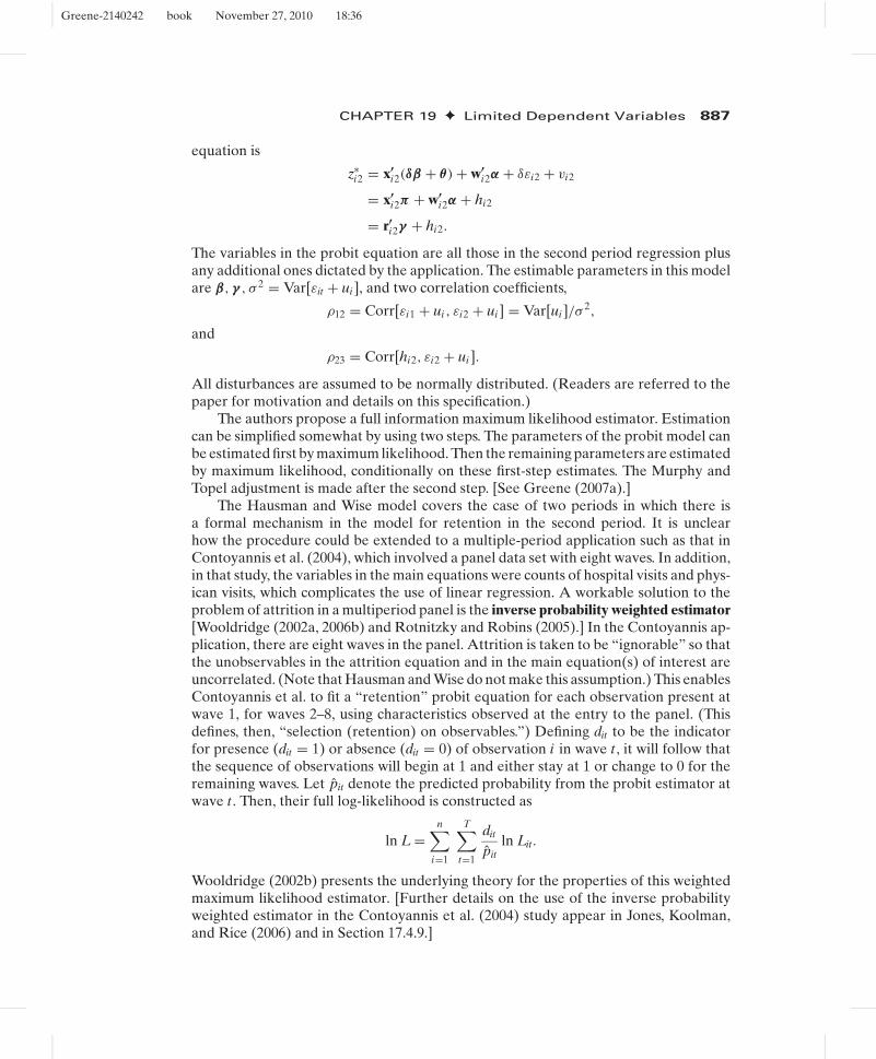
Greene-2140242 book November 27, 2010 18:36
CHAPTER 19 ✦ Limited Dependent Variables 887
equation is
z∗i2 = x′
i2(δβ + θ) + w′i2α + δεi2 + vi2
= x′i2π + w′
i2α + hi2
= r′i2γ + hi2.
The variables in the probit equation are all those in the second period regression plusany additional ones dictated by the application. The estimable parameters in this modelare β, γ , σ 2 = Var[εit + ui ], and two correlation coefficients,
ρ12 = Corr[εi1 + ui , εi2 + ui ] = Var[ui ]/σ 2,
and
ρ23 = Corr[hi2, εi2 + ui ].
All disturbances are assumed to be normally distributed. (Readers are referred to thepaper for motivation and details on this specification.)
The authors propose a full information maximum likelihood estimator. Estimationcan be simplified somewhat by using two steps. The parameters of the probit model canbe estimated first by maximum likelihood. Then the remaining parameters are estimatedby maximum likelihood, conditionally on these first-step estimates. The Murphy andTopel adjustment is made after the second step. [See Greene (2007a).]
The Hausman and Wise model covers the case of two periods in which there isa formal mechanism in the model for retention in the second period. It is unclearhow the procedure could be extended to a multiple-period application such as that inContoyannis et al. (2004), which involved a panel data set with eight waves. In addition,in that study, the variables in the main equations were counts of hospital visits and phys-ican visits, which complicates the use of linear regression. A workable solution to theproblem of attrition in a multiperiod panel is the inverse probability weighted estimator[Wooldridge (2002a, 2006b) and Rotnitzky and Robins (2005).] In the Contoyannis ap-plication, there are eight waves in the panel. Attrition is taken to be “ignorable” so thatthe unobservables in the attrition equation and in the main equation(s) of interest areuncorrelated. (Note that Hausman and Wise do not make this assumption.) This enablesContoyannis et al. to fit a “retention” probit equation for each observation present atwave 1, for waves 2–8, using characteristics observed at the entry to the panel. (Thisdefines, then, “selection (retention) on observables.”) Defining dit to be the indicatorfor presence (dit = 1) or absence (dit = 0) of observation i in wave t , it will follow thatthe sequence of observations will begin at 1 and either stay at 1 or change to 0 for theremaining waves. Let pit denote the predicted probability from the probit estimator atwave t . Then, their full log-likelihood is constructed as
ln L =n∑
i=1
T∑t=1
dit
pitln Lit.
Wooldridge (2002b) presents the underlying theory for the properties of this weightedmaximum likelihood estimator. [Further details on the use of the inverse probabilityweighted estimator in the Contoyannis et al. (2004) study appear in Jones, Koolman,and Rice (2006) and in Section 17.4.9.]

Greene-2140242 book November 27, 2010 18:36
888 PART IV ✦ Cross Sections, Panel Data, and Microeconometrics
19.6 EVALUATING TREATMENT EFFECTS
The leading recent application of models of selection and endogeneity is the evaluationof “treatment effects.” The central focus is on analysis of the effect of participationin a treatment, T, on an outcome variable, y—examples include job training programs[LaLonde (1986), Business Week (2009; Example 19.14)] and education [e.g., test scores,Angrist and Lavy (1999), Van der Klaauw (2002)]. Wooldridge and Imbens (2009, pp.22–23) cite a number of labor market applications. Recent more narrow examples in-clude Munkin and Trivedi’s (2007) analysis of the effect of dental insurance and Jonesand Rice’s (2010) survey that notes a variety of techniques and applications in healtheconomics.
Example 19.14 German Labor Market Interventions“Germany long had the highest ratio of unfilled jobs to unemployed people in Europe. Then, in2003, Berlin launched the so-called Hartz reforms, ending generous unemployment benefitsthat went on indefinitely. Now payouts for most recipients drop sharply after a year, spurringpeople to look for work. From 12.7% in 2005, unemployment fell to 7.1% last November.Even now, after a year of recession, Germany’s jobless rate has risen to just 8.6%.
At the same time, lawmakers introduced various programs intended to make it easier forpeople to learn new skills. One initiative instructed the Federal Labor Agency, which had tra-ditionally pushed the long-term unemployed into government-funded make-work positions,to cooperate more closely with private employers to create jobs. That program last year paidDutch staffing agency Randstad to teach 15,000 Germans information technology, businessEnglish, and other skills. And at a Daimler truck factory in Worth, 55 miles west of Stuttgart,several dozen short-term employees at risk of being laid off got government help to continueworking for the company as mechanic trainees.
Under a second initiative, Berlin pays part of the wages of workers hired from the ranksof the jobless. Such payments make employers more willing to take on the costs of trainingnew workers. That extra training, in turn, helps those workers keep their jobs after the aidexpires, a study by the government-funded Institute for Employment Research found. CafeNenninger in the city of Kassel, for instance, used the program to train an unemployed singlemother. Co-owner Verena Nenninger says she was willing to take a chance on her in partbecause the government picked up about a third of her salary the first year. ‘It was veryhelpful, because you never know what’s going to happen,’ Nenninger says” [Business Week(2009)].
Empirical measurement of treatment effects, such as the impact of going to collegeor participating in a job training program, presents a large variety of econometric com-plications. The natural, ultimate objective of an analysis of a “treatment” or interventionwould be the “effect of treatment on the treated.” For example, what is the effect of acollege education on the lifetime income of someone who goes to college? Measuringthis effect econometrically encounters at least two compelling computations:
Endogeneity of the treatment: The analyst risks attributing to the treatment causaleffects that should be attributed to factors that motivate both the treatment and theoutcome. In our example, the individual who goes to college might well have succeeded(more) in life than their counterpart who did not go to college even if they (themselves)did not attend college.
Missing counterfactual: The preceding thought experiment is not actually the effectwe wish to measure. In order to measure the impact of college attendance on lifetimeearnings in a pure sense, we would have to run an individual’s lifetime twice, once with
Greene-2140242 book November 27, 2010 18:36
CHAPTER 19 ✦ Limited Dependent Variables 889
college attendance and once without. Any individual is observed in only one of the twostates, so the pure measurement is impossible.
Accommodating these two problems forms the focal point of this enormous andstill growing literature. Rubin’s causal model (1974, 1978) provides a useful frameworkfor the analysis. Every individual in a population has a potential outcome, y and can beexposed to the treatment, C. We will denote by Ci the indicator whether or not the in-dividual receives the treatment. Thus, the potential outcomes are yi | (Ci = 1) = yi1 andyi | (Ci = 0) = yi0. The average treatment effect, averaged across the entire population is
ATE = E[yi1 − yi0].
The compelling complication is that the individual will exist in only one of the two states,so it is not possible to estimate ATE without further assumptions. More specifically, whatthe researcher would prefer see is the average treatment effect on the treated,
ATET = E[yi1 − yi0 | Ci = 1]
and note that the second term is the missing counterfactual.One of the major themes of the recent research is to devise robust methods of
estimation that do not rely heavily on fragile assumptions such as identification byfunctional form (e.g., relying on bivariate normality) and identification by exclusionrestrictions (e.g., relying on basic instrumental variable estimators). This is a challengingexercise—we have relied heavily on these assumptions in most of the work in thisbook up to this point. For purposes of the general specification, we will denote by xthe exogenous information that will be brought to bear on this estimation problem.The vector x may (usually will) be a set of variables that will appear in a regressionmodel, but it is useful to think more generally than that and consider x rather to be aninformation set. Certain minimal assumptions are necessary to make any headway atall. The following appear at different points in the analysis.
Conditional independence: Receiving the treatment, Ci , does not depend on theoutcome variable once the effect of x on the outcome is accounted for. If assignment tothe treatment group is completely random, then we would omit the effect of x in thisassumption. This assumption is extended for regression approaches with the conditionalmean assumption: E[yi0 | xi , Ci = 1] = E[yi0 | xi , Ci = 0] = E[yi0 | x]. This states thatthe outcome in the untreated state does not affect the participation.
Distribution of potential outcomes: The model that is used for the outcomes is thesame for treated and nontreated, f (y | x, T = 1) = f (y | x, T = 0). In a regressioncontext, this would mean that the same regression applies in both states and that thedisturbance is uncorrelated with T, or that T is exogenous. This is a very strong as-sumption that we will relax later. For the present, it removes one of the complica-tions noted previously, so a step in the model-building exercise will be to relax thisassumption.
Overlap assumption: For any value of x, 0 < Prob(Ci = 1 | x) < 1. The strict inequal-ity in this assumption means that for any x, the population will contain a mix of treatedand nontreated individuals. The usefulness of the overlap assumption is that with it, wecan expect to find, for any treated individual, an individual who looks like them but isnot treated. This assumption will be useful for regression approaches.
Greene-2140242 book November 27, 2010 18:36
890 PART IV ✦ Cross Sections, Panel Data, and Microeconometrics
The following sections will describe three major parts of the research agenda ontreatment effects: regression analysis with control functions in Section 19.6.1, propensityscore matching in Section 19.6.2, and regression discontinuity design in Section 19.6.3. Afourth area, instrumental variable estimation, was developed in Chapter 8. As noted, thisis a huge and rapidly growing literature. For example, Imbens and Wooldridge’s (2009)survey paper runs 85 pages and includes nearly 300 references, most of them since 2000.Our purpose here is to provide some of the vocabulary and a superficial introductionto methods. The survey papers by Imbens and Wooldridge (2009) and Jones and Rice(2010) provide greater detail. The conference volume by Millment, Smith, and Vytlacil(2008) contains many theoretical contributions and empirical applications.33 A Journalof Business and Economic Statistics symposium [Angrist (2001)] raised many of theimportant questions on whether and how it is possible to measure treatment effects.
19.6.1 REGRESSION ANALYSIS OF TREATMENT EFFECTS
The basic model of selectivity outlined earlier has been extended in an impressive varietyof directions. An interesting application that has found wide use is the measurement oftreatment effects and program effectiveness.
An earnings equation that accounts for the value of a college education is
earningsi = x′iβ + δCi + εi ,
where Ci is a dummy variable indicating whether or not the individual attended college.The same format has been used in any number of other analyses of programs, experi-ments, and treatments. The question is: Does δ measure the value of a college education(assuming that the rest of the regression model is correctly specified)? The answer isno if the typical individual who chooses to go to college would have relatively highearnings whether or not he or she went to college. The problem is one of self-selection.If our observation is correct, then least squares estimates of δ will actually overestimatethe treatment effect. The same observation applies to estimates of the treatment effectsin other settings in which the individuals themselves decide whether or not they willreceive the treatment.
To put this in a more familiar context, suppose that we model program participation(e.g., whether or not the individual goes to college) as
C∗i = w′
iγ + ui ,
Ci = 1 if C∗i > 0, 0 otherwise.
We also suppose that, consistent with our previous conjecture, ui and εi are correlated.Coupled with our earnings equation, we find that
E [yi | Ci = 1, xi , wi ] = x′iβ + δ + E [εi | Ci = 1, xi , wi ]
= x′iβ + δ + ρσελ(−w′
iγ )(19-34)
once again. [See (19-24).] Evidently, a viable strategy for estimating this model is to usethe two-step estimator discussed earlier. The net result will be a different estimate of δ
33In the initial essay in the volume, Goldberger (2008) reproduces Goldberger (1972) in which the authorexplores the endogeneity issue in detail with specific reference to the Head Start program of the 1960s.

Greene-2140242 book November 27, 2010 18:36
CHAPTER 19 ✦ Limited Dependent Variables 891
that will account for the self-selected nature of program participation. For nonpartici-pants, the counterpart to (19-34) is
E [yi | Ci = 0, xi , wi ] = x′iβ + ρσε
[ −φ(w′iγ )
1 − �(w′iγ )
]. (19-35)
The difference in expected earnings between participants and nonparticipants is, then,
E [yi | Ci = 1, xi , wi ] − E [yi | Ci = 0, xi , wi ] = δ + ρσε
[φi
�i (1 − �i )
]. (19-36)
If the selectivity correction λi is omitted from the least squares regression, then thisdifference is what is estimated by the least squares coefficient on the treatment dummyvariable. But because (by assumption) all terms are positive, we see that least squaresoverestimates the treatment effect. Note, finally, that simply estimating separate equa-tions for participants and nonparticipants does not solve the problem. In fact, doingso would be equivalent to estimating the two regressions of Example 19.12 by leastsquares, which, as we have seen, would lead to inconsistent estimates of both sets ofparameters.
To describe the problem created by selection on the unobservables, we will dropthe independence assumptions. The model with endogenous participation and differentoutcome equations would be
C∗i = w′
iγ + ui , Ci = 1 if C∗i > 0 and 0 otherwise,
yi0 = x′iβ0 + εi0,
yi1 = x′iβ1 + εi1.
It is useful to combine the second and third equations in
yi j = Ci (x′iβ1 + εi1) + (1 − Ci )(x′
iβ0 + εi0), j = 0, 1.
We assume joint normality for the three disturbances;⎛⎝ui
εi0
εi1
⎞⎠ ∼ N
⎡⎣
⎛⎝0
00
⎞⎠ ,
⎛⎝ 1 ρ0θ0 ρ1θ1
ρ0θ0 θ20 θ01
ρ1θ1 θ01 θ21
⎞⎠
⎤⎦ .
The variance in the participation equation is normalized to one for a binary outcome,as described earlier (Section 17.2). Endogeneity of the participation is implied by thenonzero values of the correlations ρ0 and ρ1. The familiar problem of the missing coun-terfactual appears here in our inability to estimate θ01. The data will never containinformation on both states simultaneously, so it will be impossible to estimate a co-variance of yi0 and yi1 (conditioned on xi or otherwise). Thus, the parameter θ01 is notidentified (estimable)—we normalize it to zero. The parameters of this model after thetwo normalizations can be estimated by two-step least squares as suggested in Section19.XX, or by full information maximum likelihood. The average treatment effect onthe treated would be
ATET = E[yi1 | Ci = 1, xi , wi ] − E[yi0 | Ci = 1, xi , wi ]
= x′i (β1 − β0) + (ρ1θ1 − ρ0θ0)
φ(w′
iγ)
�(w′
iγ) .

Greene-2140242 book November 27, 2010 18:36
892 PART IV ✦ Cross Sections, Panel Data, and Microeconometrics
[See (19-34).] If the treatment assignment is completely random, then ρ1 = ρ0 = 0, andwe are left with the first term. But, of course, it is the nonrandomness of the treatmentassignment that brought us to this point. Finally, if the two coefficient vectors differ onlyin their constant terms, β0,0 and β1,0, then we are left with the same δ that appears in(19-36)—the ATET would be β0,1 + Ci (β1,0 − β0,0).
There are many variations of this model in the empirical literature. They have beenapplied to the analysis of education,34 the Head Start program,35 and a host of othersettings.36 This strand of literature is particularly important because the use of dummyvariable models to analyze treatment effects and program participation has a longhistory in empirical economics. This analysis has called into question the interpretationof a number of received studies.
19.6.1.a The Normality Assumption
Some research has cast some skepticism on the selection model based on the normaldistribution. [See Goldberger (1983) for an early salvo in this literature.] Among thefindings are that the parameter estimates are surprisingly sensitive to the distributionalassumption that underlies the model. Of course, this fact in itself does not invalidate thenormality assumption, but it does call its generality into question. On the other hand,the received evidence is convincing that sample selection, in the abstract, raises seriousproblems, distributional questions aside. The literature—for example, Duncan (1986b),Manski (1989, 1990), and Heckman (1990)—has suggested some promising approachesbased on robust and nonparametric estimators. These approaches obviously have thevirtue of greater generality. Unfortunately, the cost is that they generally are quitelimited in the breadth of the models they can accommodate. That is, one might gainthe robustness of a nonparametric estimator at the cost of being unable to make use ofthe rich set of accompanying variables usually present in the panels to which selectivitymodels are often applied. For example, the nonparametric bounds approach of Manski(1990) is defined for two regressors. Other methods [e.g., Duncan (1986b)] allow moreelaborate specifications.
Recent research includes specific attempts to move away from the normality as-sumption.37 An example is Martins (2001), building on Newey (1991), which takes thecore specification as given in (19-22) as the platform but constructs an alternative to theassumption of bivariate normality. Martins’s specification modifies the Heckman modelby employing an equation of the form
E [yi | zi = 1, xi , wi ] = x′iβ + μ(w′
iγ )
where the latter “selectivity correction” is not the inverse Mills ratio, but some otherresult from a different model. The correction term is estimated using the Klein andSpady model discussed in Section 23.6.1. This is labeled a “semiparametric” approach.Whether the conditional mean in the selected sample should even remain a linear indexfunction remains to be settled. Not surprisingly, Martins’s results, based on two-step
34Willis and Rosen (1979).35Goldberger (1972, 2008).36A useful summary of the issues is Barnow, Cain, and Goldberger (1981). See, also, Imbens and Wooldridge(2009).37Again, Angrist (2001) is an important contribution to this literature.
Bill
Line
Bill
Line
Bill
Line
Bill
Sticky Note
replace with Spady's (1993) semiparametric binary choice estimator.

Greene-2140242 book November 27, 2010 18:36
CHAPTER 19 ✦ Limited Dependent Variables 893
least squares differ only slightly from the conventional results based on normality. Thisapproach is arguably only a fairly small step away from the tight parameterization of theHeckman model. Other non- and semiparametric specifications, for example, Honoreand Kyriazidou (1997, 2000) represent more substantial departures from the normalmodel, but are much less operational.38 The upshot is that the issue remains unsettled.For better or worse, the empirical literature on the subject continues to be dominatedby Heckman’s original model built around the joint normal distribution.
19.6.1.b Estimating the Effect of Treatment on the Treated
Consider a regression approach to analyzing treatment effects in a two-period setting,
yit = θt + x′itβ + γ Ci + ui + εit, t = 0, 1,
where Ci is the treatment dummy variable and ui is the unobserved individual effect.The setting is the pre- and posttreatment analysis of the sort considered in this section,where we examine the impact of a job training program on post training earnings.Because there are two periods, a natural approach to the analysis is to examine thechanges,
�yi = (θ1 − θ0) + γ�Ci + (�xit)′β + �εit
where �Ci = 1 for the treated and 0 for the nontreated individuals, and the first differ-ences eliminate the unobserved individual effects. In the absence of controls (regressors,xit), or assuming that the controls are unchanged, the estimator of the effect of the treat-ment will be
γ = �y | (�Ci = 1) − �y | (Ci = 0),
which is the difference in differences estimator. This simplifies the problem considerablybut has several shortcomings. Most important, by using the simple differences, we havelost our ability to discern what induced the change, whether it was the program orsomething else, presumably in xit.
Even without the normality assumption, the preceding regression approach is moretightly structured than many are comfortable with. A considerable amount of researchhas focused on what assumptions are needed to reach that model and whether they arelikely to be appropriate in a given setting.39 The overall objective of the analysis of thepreceding two sections is to evaluate the effect of a treatment, Ci , on the individualtreated. The implicit counterfactual is an observation on what the “response” (depen-dent variable) of the treated individual would have been had they not been treated.But, of course, an individual will be in one state or the other, not both. Denote by y0
the random variable that is the outcome variable in the absence of the treatment andby y1 the outcome when the treatment has taken place. The average treatment effect,
38This particular work considers selection in a “panel” (mainly two periods). But, the panel data setting forsample selection models is more involved than a cross-section analysis. In a panel data set, the “selection” islikely to be a decision at the beginning of Period 1 to be in the data set for all subsequent periods. As such,something more intricate than the model we have considered here is called for.39A sampling of the more important parts of the literature on this issue includes Heckman (1992, 1997),Imbens and Angrist (1994), Manski (1996), and Wooldridge (2002a, Chapter 18).
Bill
Sticky Note
comma
Bill
Line
Bill
Line
Bill
Line
Bill
Line
Bill
Line
Bill
Line
Bill
Line
Bill
Line
Bill
Line
Bill
Line
Bill
Line
Bill
Line
Bill
Sticky Note
add brackets

Greene-2140242 book November 27, 2010 18:36
894 PART IV ✦ Cross Sections, Panel Data, and Microeconometrics
averaged over the entire population is
ATE = E[y1 − y0].
This is the impact of the treatment on an individual drawn at random from the entirepopulation. However, the desired quantity is not necessarily the ATE, but the averagetreatment effect on the treated, which would be
ATE |T = E[y1 − y0 | C = 1].
The difficulty of measuring this is, once again, the counterfactual, E[y0 | C = 1]. Whetherthese two measures will be the same is at the center of the much of the discussionon this subject. If treatment is completely randomly assigned, then E[yj | C = 1] =E[yj | C = 0] = E[yj | C = j], j = 0, 1. This means that with completely randomtreatment assignment
ATE = E[y1 | C = 1] − E[y0 | C = 0].
To put this in our example, if college attendance were completely randomly distributedthroughout the population, then the impact of college attendance on income (neglectingother covariates at this point) could be measured simply by averaging the incomes ofcollege attendees and subtracting the average income of nonattendees. The precedingtheory might work for the treatment “having brown eyes,” but it is unlikely to workfor college attendance. Not only is the college attendance treatment not randomlydistributed, but the treatment “assignment” is surely related to expectations about y1
versus y0, and, at a minimum, y0 itself. (College is expensive.) More generally, theresearcher faces the difficulty in calculating treatment effects that assignment to thetreatment might not be exogenous.
The control function approach that we used in (19-34)–(19-36) is used to accountfor the endogeneity of the treatment assignment in the regression context. The veryspecific assumptions of the bivariate normal distribution of the unobservables some-what simplifies the estimation, because they make explicit what control function (λi )
is appropriate to use in the regression. As Wooldridge (2002a, p. 622) points out, how-ever, the binary variable in the treatment effects regression represents simply an en-dogenous variable in a linear equation, amenable to instrumental variable estimation(assuming suitable instruments are available). Barnow, Cain, and Goldberger (1981)proposed a two-stage least squares estimator, with instrumental variable equal to thepredicted probability from the probit treatment assignment model. This is slightly lessparametric than (19-36) because, in principle, its validity does not rely on joint nor-mality of the disturbances. [Wooldridge (2002a, pp. 621–633) discusses the underlyingassumptions.
19.6.2 PROPENSITY SCORE MATCHING
If the treatment assignment is “completely ignorable,” then, as noted, estimation ofthe treatment effects is greatly simplified. Suppose, as well, that there are observablevariables that influence both the outcome and the treatment assignment. Suppose itis possible to obtain pairs of individuals matched by a common xi , one with Ci = 0,the other with Ci = 1. If done with a sufficient number of pairs so as to average
Bill
Sticky Note
delete "["

Greene-2140242 book November 27, 2010 18:36
CHAPTER 19 ✦ Limited Dependent Variables 895
over the population of xi ’s, then a matching estimator, the average value of (yi | Ci =1) − (yi | Ci = 0), would estimate E[y1 − y0], which is what we seek. Of course, itis optimistic to hope to find a large sample of such matched pairs, both because thesample overall is finite and because there may be many regressors, and the “cells” inthe distribution of xi are likely to be thinly populated. This will be worse when theregressors are continuous, for example, with a “family income” variable. Rosenbaumand Rubin (1983) and others40 suggested, instead, matching on the propensity score,F(xi ) = Prob(Ci = 1 | xi ). Individuals with similar propensity scores are paired andthe average treatment effect is then estimated by the differences in outcomes. Variousstrategies are suggested by the authors for obtaining the necessary subsamples and forverifying the conditions under which the procedures will be valid. [See, e.g., Becker andIchino (2002) and Greene (2007c).]
Example 19.15 Treatment Effects on EarningsLaLonde (1986) analyzed the results of a labor market experiment, The National SupportedWork Demonstration, in which a group of disadvantaged workers lacking basic job skills weregiven work experience and counseling in a sheltered environment. Qualified applicants wereassigned to training positions randomly. The treatment group received the benefits of theprogram. Those in the control group “were left to fend for themselves.” [The demonstrationwas run in numerous cities in the mid-1970s. See LaLonde (1986, pp. 605–609) for detailson the NSW experiments.] The training period was 1976–1977; the outcome of interest forthe sample examined here was posttraining 1978 earnings. LaLonde reports a large varietyof estimates of the treatment effect, for different subgroups and using different estimationmethods. Nonparametric estimates for the group in our sample are roughly $900 for theincome increment in the posttraining year. (See LaLonde, p. 609.) Similar results are reportedfrom a two-step regression-based estimator similar to (19-34) to (19-36). (See LaLonde’sfootnote to Table 6, p. 616.)
LaLonde’s data are fairly well traveled, having been used in replications and extensionsin, for example, Dehejia and Wahba (1999), Becker and Ichino (2002), and Greene (2007b, c).We have reestimated the matching estimates reported in Becker and Ichino. The data in thefile used there (and here) contain 2,490 control observations and 185 treatment observationson the following variables:
t = treatment dummy variableage = age in years
educ = education in yearsmarr = dummy variable for married
black = dummy variable for blackhisp = dummy variable for Hispanic
nodegree = dummy for no degree (not used)re74 = real earnings in 1974re75 = real earnings in 1975re78 = real earnings in 1978
40Other important references in this literature are Becker and Ichino (1999), Dehejia and Wahba (1999),LaLonde (1986), Heckman, Ichimura, and Todd (1997, 1998), Heckman, Ichimura, Smith, and Todd (1998),Heckman, LaLonde, and Smith (1999), Heckman, Tobias, and Vytlacil (2003), and Heckman and Vytlacil(2000).
Bill
Sticky Note
commas at ends of lines
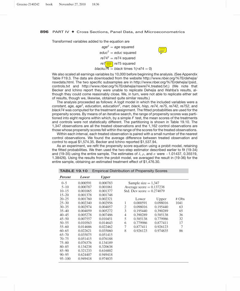
Greene-2140242 book November 27, 2010 18:36
896 PART IV ✦ Cross Sections, Panel Data, and Microeconometrics
Transformed variables added to the equation are
age2 = age squared
educ2 = educ squared
re742 = re74 squared
re752 = re75 squaredblacku74 = black times 1(r e74 = 0)
We also scaled all earnings variables by 10,000 before beginning the analysis. (See AppendixTable F19.3. The data are downloaded from the website http://www.nber.org/%7Erdehejia/nswdata.html. The two specific subsamples are in http://www.nber.org/%7Erdehejia//psidcontrols.txt and http://www.nber.org/%7Erdehejia/nswre74 treated.txt.) (We note thatBecker and Ichino report they were unable to replicate Dehejia and Wahba’s results, al-though they could come reasonably close. We, in turn, were not able to replicate either setof results, though we, likewise, obtained quite similar results.)
The analysis proceeded as follows: A logit model in which the included variables were aconstant, age, age2, education, education2, marr, black, hisp, re74, re75, re742, re752, andblack74 was computed for the treatment assignment. The fitted probabilities are used for thepropensity scores. By means of an iterative search, the range of propensity scores was parti-tioned into eight regions within which, by a simple F test, the mean scores of the treatmentsand controls were not statistically different. The partitioning is shown in Table 19.10. The1,347 observations are all the treated observations and the 1,162 control observations arethose whose propensity scores fell within the range of the scores for the treated observations.
Within each interval, each treated observation is paired with a small number of the nearestcontrol observations. We found the average difference between treated observation andcontrol to equal $1,574.35. Becker and Ichino reported $1,537.94.
As an experiment, we refit the propensity score equation using a probit model, retainingthe fitted probabilities. We then used the two-step estimator described earlier to fit (19-34)and (19-35) using the entire sample. The estimates of δ, ρ, and σ were −1.01437, 0.35519,1.38426). Using the results from the probit model, we averaged the result in (19-36) for theentire sample, obtaining an estimated treatment effect of $1,476.30.
TABLE 19.10 Empirical Distribution of Propensity Scores
Percent Lower Upper
0–5 0.000591 0.000783 Sample size = 1,3475–10 0.000787 0.001061 Average score = 0.137238
10–15 0.001065 0.001377 Std. Dev score = 0.27407915–20 0.001378 0.00174820–25 0.001760 0.002321 Lower Upper # Obs25–30 0.002340 0.002956 1 0.000591 0.098016 104130–35 0.002974 0.004057 2 0.098016 0.195440 6335–40 0.004059 0.005272 3 0.195440 0.390289 6540–45 0.005278 0.007486 4 0.390289 0.585138 3645–50 0.007557 0.010451 5 0.585138 0.779986 3250–55 0.010563 0.014643 6 0.779986 0.877411 1755–60 0.014686 0.022462 7 0.877411 0.926123 760–65 0.022621 0.035060 8 0.926123 0.974835 8665–70 0.035075 0.05141570–75 0.051415 0.07618875–80 0.076376 0.13418980–85 0.134238 0.32063885–90 0.321233 0.61600290–95 0.624407 0.94941895–100 0.949418 0.974835
Bill
Sticky Note
commas at ends of lines, period at end of last line
Bill
Sticky Note
delete "u"

Greene-2140242 book November 27, 2010 18:36
CHAPTER 19 ✦ Limited Dependent Variables 897
19.6.3 REGRESSION DISCONTINUITY
There are many situations in which there is no possibility of randomized assignmentof treatments. Examples include student outcomes and policy interventions in schools.Angrist and Lavy (1999), for example, studied the effect of class sizes on test scores.Van der Klaauw studied financial aid offers that were tied to SAT scores and gradepoint averages. In these cases, the natural experiment approach advocated by Angristand Pischke (2009) is an appealing way to proceed, when it is feasible. The regressiondiscontinuity design presents an alternative strategy. The conditions under which theapproach can be effective are when (1) the outcome, y, is a continuous variable; (2) theoutcome varies smoothly with an assignment variable, A, and (3) treatment is “sharply”assigned based on the value of A, specifically C = 1(A > A∗) where A∗ is a fixedthreshold or cutoff value. [A “fuzzy design is based on Prob(C = 1 | A) = F(A). Theidentification problems with fuzzy design are much more complicated than with sharpdesign. Readers are referred to Van der Klaauw (2002) for further discussion of fuzzydesign.] We assume, then, that
y = f (A, C) + ε.
Suppose, for example, the outcome variable is a test score, and that an administrativetreatment such as a special education program is funded based on the poverty rates ofcertain communities. The ideal conditions for a regression discontinuity design based onthese assumptions is shown in Figure 19.8. The logic of the calculation is that the pointsnear the threshold value, which have “essentially” the same stimulus value, constitutea nearly random sample of observations which are segmented by the treatment.
The method requires that E[ε | A, C] = E[ε | A]—the assignment variable—be ex-ogenous to the experiment. The result in Figure 19.8 is consistent with
y = f (A) + αC + ε,
FIGURE 19.8 Regression Discontinuity.
Rate
RD EstimatedTreatment Effect
2
4
6
8
10
12
02 3 4 5 6 71
Scor
e
Greene-2140242 book November 27, 2010 18:36
898 PART IV ✦ Cross Sections, Panel Data, and Microeconometrics
where α will be the treatment effect to be estimated. The specification of f (A) canbe problematic; assuming a linear function when something more general will bias theestimate of α. For this reason, nonparametric methods, such as the LOWESS regression(see Section 12.3.5) might be attractive. This is likely to enable the analyst to make fulleruse of the observations that are more distant from the cutoff point. [See Van der Klaaus(2002).] Identification of the treatment effect begins with the assumption that f (A) iscontinuous at A∗, so that
limA↑A∗ f (A) = lim
A↓A∗ f (A) = f (A∗).
Then
limA↓A∗ E[y | A] − lim
A↑A∗ E[y | A] = f (A∗) + α + limA↓A∗ E[ε | A] − f (A∗) − lim
A↑A∗ E[ε | A]
= α.
With this in place, the treatment effect can be estimated by the difference of the averageoutcomes for those individuals “close” to the threshold value, A∗. Details on regressiondiscontinuity design are provided by Trochim (1984, 2000) and Van der Klaauw (2002).
19.7 SUMMARY AND CONCLUSIONS
This chapter has examined settings in which, in principle, the linear regression model ofChapter 2 would apply, but the data generating mechanism produces a nonlinear form:truncation, censoring, and sample selection or endogenous sampling. For each case, wedevelop the basic theory of the effect and then use the results in a major area of researchin econometrics.
In the truncated regression model, the range of the dependent variable is restrictedsubstantively. Certainly all economic data are restricted in this way—aggregate incomedata cannot be negative, for example. But when data are truncated so that plausiblevalues of the dependent variable are precluded, for example, when zero values for ex-penditure are discarded, the data that remain are analyzed with models that explicitlyaccount for the truncation. The stochastic frontier model is based on a composite dis-turbance in which one part follows the assumptions of the familiar regression modelwhile the second component is built on a platform of the truncated regression.
When data are censored, values of the dependent variable that could in principle beobserved are masked. Ranges of values of the true variable being studied are observedas a single value. The basic problem this presents for model building is that in sucha case, we observe variation of the independent variables without the correspondingvariation in the dependent variable that might be expected. Consistent estimation,and useful interpretation of estimation results are based on maximum likelihood orsome other technique that explicitly accounts for the censoring mechanism. The mostcommon case of censoring in observed data arises in the context of duration analysis,or survival functions (which borrows a term from medical statistics where this styleof model building originated). It is useful to think of duration, or survival data, asthe measurement of time between transitions or changes of state. We examined threemodeling approaches that correspond to the description in Chapter 12; nonparametric(survival tables), semiparametric (the proportional hazard models), and parametric(various forms such as the Weibull model).
Bill
Sticky Note
insert "is appropriate" before "will"

Greene-2140242 book November 27, 2010 18:36
CHAPTER 19 ✦ Limited Dependent Variables 899
Finally, the issue of sample selection arises when the observed data are not drawnrandomly from the population of interest. Failure to account for this nonrandom sam-pling produces a model that describes only the nonrandom subsample, not the largerpopulation. In each case, we examined the model specification and estimation tech-niques which are appropriate for these variations of the regression model. Maximumlikelihood is usually the method of choice, but for the third case, a two-step estimatorhas become more common. The leading contemporary application of selection meth-ods and endogenous sampling is in the measure of treatment effects. We consideredthree approaches to analysis of treatment effects; regression methods, propensity scorematching, and regression discontinuity.
Key Terms and Concepts
• Accelerated failure timemodel
• Attenuation• Average treatment effect• Average treatment effect on
the treated• Censored regression model• Censored variable• Censoring• Conditional mean
assumption• Conditional moment test• Control function• Corner solution model• Data envelopment analysis• Degree of truncation• Delta method• Difference in differences• Duration model• Exponential• Exponential model• Fuzzy design• Generalized residual• Hazard function• Hazard rate• Heterogeneity• Heteroscedasticity
• Hurdle model• Incidental truncation• Instrumetal variable
estimation• Integrated hazard function• Inverse probability
weighted estimator• Inverse Mills ratio• Lagrange multiplier test• Matching estimator• Mean independence
assumption• Missing counterfactual• Negative duration
dependence• Olsen’s reparameterization• Parametric• Parametric model• Partial likelihood• Positive duration
dependence• Product limit estimator• Propensity score• Proportional hazard• Regression discontinuity
design• Risk set
• Rubin causal model• Sample selection• Selection on observables• Selection on unobservables• Semiparametric estimator• Semiparametric model• Specification error• Stochastic frontier model• Survival function• Time-varying covariate• Tobit model• Treatment effect• Truncated distribution• Truncated mean• Truncated normal
distribution• Truncated random variable• Truncated standard normal
distribution• Truncated variance• Truncation• Two-step estimation• Type II tobit model• Weibull model• Weibull survival model
Exercises
1. The following 20 observations are drawn from a censored normal distribution:
3.8396 7.2040 0.00000 0.00000 4.4132 8.02305.7971 7.0828 0.00000 0.80260 13.0670 4.32110.00000 8.6801 5.4571 0.00000 8.1021 0.000001.2526 5.6016

Greene-2140242 book November 27, 2010 18:36
900 PART IV ✦ Cross Sections, Panel Data, and Microeconometrics
The applicable model is
y∗i = μ + εi ,
yi = y∗i if μ + εi > 0, 0 otherwise,
εi ∼ N[0, σ 2].
Exercises 1 through 4 in this section are based on the preceding information. TheOLS estimator of μ in the context of this tobit model is simply the sample mean.Compute the mean of all 20 observations. Would you expect this estimator to over-or underestimate μ? If we consider only the nonzero observations, then the trun-cated regression model applies. The sample mean of the nonlimit observationsis the least squares estimator in this context. Compute it and then comment onwhether this sample mean should be an overestimate or an underestimate of the truemean.
2. We now consider the tobit model that applies to the full data set.a. Formulate the log-likelihood for this very simple tobit model.b. Reformulate the log-likelihood in terms of θ = 1/σ and γ = μ/σ . Then derive
the necessary conditions for maximizing the log-likelihood with respect to θ
and γ .c. Discuss how you would obtain the values of θ and γ to solve the problem in
part b.d. Compute the maximum likelihood estimates of μ and σ .
3. Using only the nonlimit observations, repeat Exercise 2 in the context of the trun-cated regression model. Estimate μ and σ by using the method of moments esti-mator outlined in Example 19.2. Compare your results with those in the previousexercises.
4. Continuing to use the data in Exercise 1, consider once again only the nonzeroobservations. Suppose that the sampling mechanism is as follows: y∗ and anothernormally distributed random variable z have population correlation 0.7. The twovariables, y∗ and z, are sampled jointly. When z is greater than zero, y is re-ported. When z is less than zero, both z and y are discarded. Exactly 35 drawswere required to obtain the preceding sample. Estimate μ and σ. (Hint: Use Theo-rem 19.5.)
5. Derive the partial effects for the tobit model with heteroscedasticity that is de-scribed in Section 19.3.5.a.
6. Prove that the Hessian for the tobit model in (19-14) is negative definite afterOlsen’s transformation is applied to the parameters.
Applications
1. We examined Ray Fair’s famous analysis (Journal of Political Economy, 1978) of aPsychology Today survey on extramarital affairs in Example 18.9 using a Poissonregression model. Although the dependent variable used in that study was a count,Fair (1978) used the tobit model as the platform for his study. You can reproducethe tobit estimates in Fair’s paper easily with any software package that containsa tobit estimator—most do. The data appear in Appendix Table F18.1. Reproduce

Greene-2140242 book November 27, 2010 18:36
CHAPTER 19 ✦ Limited Dependent Variables 901
Fair’s least squares and tobit estimates. Compute the partial effects for the modeland interpret all results.
2. Fair’s original study also included but did not analyze a second data set that wasa similar survey conducted by Redbook magazine. The data are reproduced inAppendix Table F17.2. (Our thanks to Ray Fair for providing these data.) Thissample contains observations on 6,366 women and the following variables:
id = an identification number
C = constant, value = 1
yrb = a constructed measure of time spent in extramarital affairs
v1 = a rating of the marriage, coded 1 to 4
v2 = age, in years, aggregated
v3 = number of years married
v4 = number of children, top coded at 5
v5 = religiosity, 1 to 4, 1 = not, 4 = very
v6 = education, coded 9, 12, 14, 16, 17, 20
v7 = occupation
v8 = husband’s occupation
Three other variables were not used. Details on the variables in the model aregiven in Fair’s (1978) Journal of Political Economy paper. Using these data, con-duct a parallel study to the Psychology Today study that was done in Fair (1978).Are the results consistent? Report all results, including partial effects and relevantdiagnostic statistics.
3. Continuing the analysis of the previous application, note that these data conformprecisely to the description of “corner solutions” in Section 19.3.4. The dependentvariable is not censored in the fashion usually assumed for a tobit model. To inves-tigate whether the dependent variable is determined by a two-part decision process(yes/no and, if yes, how much), specify and estimate a two-equation model in whichthe first equation analyzes the binary decision A = 1 if yrb > 0 and 0 otherwiseand the second equation analyzes yrb | yrb > 0. What is the appropriate model?What do you find? Report all results. (Note: If you analyze the second dependentvariable using the truncated regression, you should remove some extreme obser-vations from your sample. The truncated regression estimator refuses to convergewith the full data set but works nicely for the example if you omit observations withyrb > 5.)
4. StochasticFrontier Model. Section 10.5.1 presents estimates of a Cobb–Douglascost function using Nerlove’s 1955 data on the U.S. electric power industry. Chris-tensen and Greene’s 1976 update of this study used 1970 data for this industry. TheChristensen and Greene data are given in Appendix Table F4.3. These data haveprovided a standard test data set for estimating different forms of production andcost functions, including the stochastic frontier model discussed in Section 19.2.4. Ithas been suggested that one explanation for the apparent finding of economies of
Bill
Sticky Note
The Mroz (1975) data used in Example 19.11 (See Appendix Table F5.1) also describe a setting in which the Tobit model has been frequently applied. The sample contains 753 observations on labor market outcomes for married women, including the following variables: lfp = indicator (0/1) for whether in the formal labor market (lfp=1) or not (lfp=0), whrs = wife's hours worked, kl6 = number of children under 6 years old in the household, k618 = number of children from 6 to 18 years old in the household, wa = wife's age, we = wife's education, ww = wife's hourly wage, hhrs = husband's hours worked, ha = husband's age, hw = husband's wage, faminc = family income from other sources, wmed = wife's mother's education wfed = wife's father's education cit = dummy variable for living in an urban area, ax = labor market experience = age - we - 5, and several variables that will not be useful here. Using these data, estimate a tobit model for the wife's hours worked. Report all results including partial effects and relevant diagnostic statistics. Repeat the analysis for the wife's labor earnings, ww times whrs.. Which is a more plausible model?
Bill
Rectangle
Bill
Sticky Note
this exercise must be replaced. See other sticky note
Bill
Sticky Note
change "A = 1 if yrb > 0" to "lfp = 1 if whrs > 0" lfp and whrs are italic
Bill
Sticky Note
change "yrb" to "whrs" both times.
Bill
Line
Bill
Line
Bill
Line
Bill
Line
Bill
Line
Bill
Line
Bill
Line
Bill
Line
Bill
Line
Bill
Sticky Note
delete
Bill
Sticky Note
F4.4
Greene-2140242 book November 27, 2010 18:36
902 PART IV ✦ Cross Sections, Panel Data, and Microeconometrics
scale in these data is that the smaller firms were inefficient for other reasons. Thestochastic frontier might allow one to disentangle these effects. Use these data tofit a frontier cost function which includes a quadratic term in log output in addi-tion to the linear term and the factor prices. Then examine the estimated Jondrowet al. residuals to see if they do indeed vary negatively with output, as suggested.(This will require either some programming on your part or specialized software.The stochastic frontier model is provided as an option in Stata, TSP, and LIMDEP.Or, the likelihood function can be programmed fairly easily for RATS, MatLab, orGAUSS. (Note: For a cost frontier as opposed to a production frontier, it is nec-essary to reverse the sign on the argument in the � function that appears in thelog-likelihood.)