Limit States and Load and Resistance Design of Slopes and ...
263
FHWA/IN/JTRP-2008/5 Final Report LIMIT STATES AND LOAD AND RESISTANCE DESIGN OF SLOPES AND RETAINING STRUCTURES Dongwook Kim Rodrigo Salgado January 2009
Transcript of Limit States and Load and Resistance Design of Slopes and ...

FHWA/IN/JTRP-2008/5
Final Report
LIMIT STATES AND LOAD AND RESISTANCE DESIGN OF SLOPES AND RETAINING STRUCTURES
Dongwook Kim Rodrigo Salgado
January 2009
62-1 1/09 JTRP-2008/5 INDOT Division of Research West Lafayette, IN 47906
INDOT Research
TECHNICAL Summary Technology Transfer and Project Implementation Information
TRB Subject Code: 62-1 Foundation Soils January 2009 Publication No. FHWA/IN/JTRP-2008/5, SPR-2634 Final Report
Limit States and Load Resistance Design of Slopes and Retaining Structures
Introduction The primary goal of this report was to develop Load and Resistance Factor Design (LRFD) methods for slopes and retaining structures. Even though there is past research on LRFD of shallow foundations and piles, there are very few publications available on LRFD of slopes and retaining structures. Most commonly, the design goal for slopes is to economically select (i) slope angle and (ii) slope protection measures that will not lead to any limit state. For retaining structures, the goal is the economical selection of the type and dimensions of the retaining structure, including of the reinforcement for MSE walls, again without violating limit state checks. The design of slopes and retaining structures has traditionally been conducted using the Working Stress Design (WSD) approach. Even in recent years, WSD has remained the primary design approach in geotechnical engineering. Within this framework, for any design problem, capacity or resistance is compared with the loading. To account for the uncertainties associated with the calculation of resistance and loading, a single factor of safety is used to divide the capacity (or, from the opposite point of view, to multiply the loading) before the comparison is made. The factor of safety is the tool that the WSD approach uses to account for uncertainties. Thus, in designs following WSD, the uncertainties are expressed using a single number: the factor of safety. Therefore, the uncertainties
related to load estimation cannot be separated from those related to resistance. The LRFD method combines the limit states design concept with the probabilistic approach, accounting for the uncertainty of parameters related to both the loads and the resistance. In the present report, only Ultimate Limit States (ULSs) are considered. An ULS is a state for which the total load is equal to the maximum resistance of the system. When the total load is equal to or higher than the maximum resistance of the system, the system “fails” (that is, fails to perform according to pre-defined criteria). To prevent failure of the system, Limit State Design (LSD) requires the engineer to identify every possible ULS and to ensure that none of those are reached. However, in the case of LRFD, which combines the probabilistic approach with LSD, the probability of failure of the system is calculated from the probability density distributions of the total load and the maximum resistance. LRFD aims to keep this probability of failure from exceeding a certain level (the target probability of failure or target reliability index). LRFD uses an LSD framework, which checks for the ULS using partial factors on loads and on resistance. These partial factors, associated with the loads and the resistance, are calculated based on the uncertainties associated with the loads and the resistance.
Findings
We have developed LRFD methods for slopes and MSE walls using limit state design concepts and probability theory. Resistance Factor (RF) values that are compatible with the LFs of the AASHTO LRFD specifications (2007) are tentatively suggested in this report for LRFD of slopes and MSE walls from the result of reliability analyses on the basis of a rational assessment of the
uncertainties of the parameters that are used in the analysis. 1. LRFD of Slopes We have successfully employed Gaussian random field theory for the representation of spatial (inherent) soil variability. The reliability analysis

62-1 1/09 JTRP-2008/5 INDOT Division of Research West Lafayette, IN 47906
program developed for LRFD of slopes using Monte Carlo simulations in conjunction with the soil parameters represented by Gaussian random fields works well and provides reliable results. Even for the given target probability of failure, geometry of slope, and mean values of parameters and their uncertainties, there is no uniqueness of the RF value for slopes. In other words, the RF value resulting from Monte Carlo simulations varies from case to case. This is because the Gaussian random fields and also the slip surface at the ULS for each random realization of a slope defined by the mean and variance values of the strength parameters and unit weights of each layer and of the live load are different from simulation to simulation. We have proposed a way to deal with this nonuniqueness that provides an acceptable basis on which to make resistance factor recommendations. 2. LRFD of MSE walls For each limit state, the First-Order Reliability Method (FORM) was successfully used to compute the values of loads and resistance at the ULS for the given target reliability index and the corresponding optimal load and resistance factors. A parametric study of the external stability (sliding and overturning) of MSE walls identified the unit weight of the retained soil as the parameter with the most impact on the RF value. This seems to be because the change of the unit weight of the retained soil results in a change of the composition of the uncertainty of the total lateral load acting on the reinforced soil. For example, if the unit weight of the retained soil increases, the ratio of the lateral load due to the live uniform surcharge load to the lateral load due to the self-weight of the retained soil decreases. Therefore, the uncertainty of the total load
decreases because the lateral load due to the live uniform surcharge load has a much higher bias factor and COV compared to those of the lateral load due to the self-weight of the retained soil. Consequently, the RF values for sliding and overturning increase as the height of the MSE wall increases. For pullout of the steel-strip reinforcement, the most important parameter on the RF value is the relative density of the reinforced soil because not only the relative density has the highest COV among all the parameters but also the mean value of the relative density has a significant influence on the pullout resistance factor. In addition, the level (or the vertical location) of the steel-strip reinforcement also has considerable impact on the RF value because the reinforcement level changes the uncertainty of total load significantly by changing the ratio of the load due to the self-weight of the reinforced soil to the load due to the live uniform surcharge load.
In this study, we found the worst cases, which have the lowest RF values, by varying the parameters within their possible ranges for different MSE wall heights and different target reliability indices. The “worst-case” RF values for sliding and overturning are given in the report. The “worst-case” RF values for pullout, which occur at the first reinforcement level from the top of the MSE wall, are suggested as RF values to use in pullout failure checks. Usually, the required reinforcement length L at the first reinforcement level from the top of an MSE wall is used for all the other reinforcement levels when the vertical and horizontal spacing of the reinforcements are the same. Therefore, in general, this required reinforcement length L can be calculated using the RF value for pullout at the first reinforcement depth z.
Implementation
RF values for LRFD of slopes and MSE walls in this report are calculated based on analyses done for a limited number of conditions. The RF values for slopes and MSE wall designs given in this report are valid only when designers use (i) the equations for load and resistance and (ii) the test methods for design parameters given in this report. The RF values are computed for two different target probability of failure (Pf = 0.001 and 0.01) for slopes and three different target reliability indices (βT=2.0, 2.5, and 3.0) for MSE walls. The higher values of target probability of failure (0.01) and the lower values of target reliability index (2.0 and 2.5) are provided for illustration purposes, as they would typically be excessively daring in most
design problems. For slope stability, resistance factors for a probability of failure lower than 0.001 would require considerable time to calculate. In practice, the importance of the structure may vary; therefore, designers should select an appropriate target probability of failure (or target reliability index), which would produce an economical design without excessive risk to the stability of a structural and geotechnical system. For development of complete and reliable sets of resistance factors for LRFD of slopes and MSE walls, we recommend the following: (1) It is necessary to perform comprehensive
research on the classification of the type of
62-1 1/09 JTRP-2008/5 INDOT Division of Research West Lafayette, IN 47906
error associated with measurements, which is a process that requires extensive effort in testing and data collection. This effort would make it possible to assess the uncertainty of systematic errors more accurately. As uncertainties in parameters reflect directly on RF values, improved assessment of these uncertainties would be very beneficial.
(2) The load factors provided in the current AASHTO LRFD specifications (2007) are equal to one regardless of the load type. This means that RF values (0.75 when the geotechnical parameters are well defined and the slope does not support or contain a structural element, and 0.65 when the geotechnical parameters are based on limited information or the slope contains or supports a structural element) proposed in the specifications are the inverse values of the factors of safety (1.3 and 1.5) that were given in the old AASHTO specifications. Thus, LRFD of slopes as currently covered by the AASHTO specifications is in effect the same as Working Stress Design (WSD). Use of the algorithm provided in this report would produce appropriate load factors that reflect the uncertainty of the corresponding loadings and allow determination of suitable resistance factors. Then, the current load and resistance factor for LRFD of slopes in the AASHTO LRFD specifications could be updated to more closely reflect the principles of LRFD.
(3) More analyses are necessary for determining RF values for slope design. The following all should be explored: (i) different geometries; (ii) different external loading conditions (load type, location, and magnitude); (iii) different combinations of soil layers; (iv) different combinations of the values of soil properties (considering wide ranges of soil property values); (v) wider ranges of probability of failure (and, in particular, lower probabilities of failure); (vi) repeatability checks to further validate the method proposed to handle the nonuniqueness of resistance and load factors resulting from different simulations.
(4) Similarly to slopes, more analyses varying
MSE wall geometry, loading condition and soil properties will be helpful to expand LRFD for MSE wall design for different site conditions.
(5) The RF value for general loss of stability of
MSE walls could be examined using the appropriate load factors determined from extensive Monte Carlo simulations for LRFD of slopes.
(6) For certain geotechnical structures, such as
levees, dams or abutments of large and massive bridges, lower target probabilities of failure (or higher target reliability index) should be considered. A more careful study of acceptable values of probability of failure should be conducted.
Contacts
For more information: Prof. Rodrigo Salgado Principal Investigator School of Civil Engineering Purdue University West Lafayette IN 47907 Phone: (765) 494-5030 Fax: (765) 496-1364 E-mail: [email protected]
Indiana Department of Transportation Division of Research 1205 Montgomery Street P.O. Box 2279 West Lafayette, IN 47906 Phone: (765) 463-1521 Fax: (765) 497-1665 Purdue University Joint Transportation Research Program School of Civil Engineering West Lafayette, IN 47907-1284 Phone: (765) 494-9310 Fax: (765) 496-7996 E-mail: [email protected] http://www.purdue.edu/jtrp

Final Report
FHWA/IN/JTRP-2008/5
LIMIT STATES AND LOAD AND RESISTANCE DESIGN OF SLOPES AND
RETAINING STRUCTURES
Dongwook Kim
Graduate Research Assistant
and
Rodrigo Salgado, P.E. Professor
Geotechnical Engineering
School of Civil Engineering Purdue University
Joint Transportation Research Program
Project No: C-36-36MM File No: 06-14-39
SPR-2634
Prepared in Cooperation with the Indiana Department of Transportation and
The U.S. Department of Transportation Federal Highway Administration
The contents of this report reflect the views of the authors who are responsible for the facts and the accuracy of the data presented herein. The contents do not necessarily reflect the official views or policies of the Federal Highway Administration and the Indiana Department of Transportation. This report does not constitute a standard, specification or regulation.
Purdue University
West Lafayette, Indiana April 2008

TECHNICAL REPORT STANDARD TITLE PAGE 1. Report No.
2. Government Accession No. 3. Recipient's Catalog No.
FHWA/IN/JTRP-2008/5
4. Title and Subtitle Limit States and Load Resistance Design of Slopes and Retaining Structures
5. Report Date January 2009
6. Performing Organization Code 7. Author(s) Dongwook Kim and Rodrigo Salgado
8. Performing Organization Report No. FHWA/IN/JTRP-2008/5
9. Performing Organization Name and Address Joint Transportation Research Program 550 Stadium Mall Drive Purdue University West Lafayette, IN 47907-2051
10. Work Unit No.
11. Contract or Grant No. SPR-2634
12. Sponsoring Agency Name and Address Indiana Department of Transportation State Office Building 100 North Senate Avenue Indianapolis, IN 46204
13. Type of Report and Period Covered
Final Report
14. Sponsoring Agency Code
15. Supplementary Notes Prepared in cooperation with the Indiana Department of Transportation and Federal Highway Administration.
16. Abstract
Load and Resistance Factor Design (LRFD) methods for slopes and MSE walls were developed based on probability theory. The complexity in developing LRFD for slopes and MSE walls results from the fact that (1) the representation of spatial variability of soil parameters of slopes using Gaussian random field is computationally demanding and (2) LRFD of MSE walls requires examination of multiple ultimate limit states for both external and internal stability checks. For each design case, a rational framework is developed accounting for different levels of target probability of failure (or target reliability index) based on the importance of the structure. The conventional equations for loads and resistance in the current MSE wall design guides are modified so that the equations more closely reproduce the ultimate limit states (ULSs) in the field with as little uncertainty as possible. The uncertainties of the parameters, the transformation and the models related to each ULS equation are assessed using data from an extensive literature review.
The framework used to develop LRFD methods for slopes and MSE walls was found to be effective. For LRFD of slopes, several slopes were considered. Each was defined by the mean value of the strength parameters and unit weight of each soil layer and of the live load. (1) Gaussian random field theory was used to generate random realizations of the slope (each realization had values of strength and unit weight that differed from the mean by a random amount), (2) a slope stability analysis was performed for each slope to find the most critical slip surface and the corresponding driving and resisting moments, (3) the probability of failure was calculated by counting the number of slope realizations for which the factor of safety did not exceed 1 and dividing that number by the total number of realizations, (4) the mean and variance of the soil parameters was adjusted and this process repeated until the calculated probability of failure was equal to the target probability of failure, and (5) optimum load and resistance factors were obtained using the ultimate limit state values and nominal values of driving and resisting moments. For LRFD of MSE walls, (1) the First-Order Reliability Method was successfully implemented for both external and internal limit states and (2) a reasonable RF value for each limit state was calculated for different levels of target reliability index.
17. Key Words Load and Resistance Factor Design (LRFD); Slope; Mechanically Stabilized Earth (MSE) wall; Reliability analysis; Gaussian random field; Monte Carlo simulation; First-Order Reliability Method (FORM).
18. Distribution Statement No restrictions. This document is available to the public through the National Technical Information Service, Springfield, VA 22161
19. Security Classif. (of this report)
Unclassified
20. Security Classif. (of this page)
Unclassified
21. No. of Pages 233
22. Price
Form DOT F 1700.7 (8-69)

ii
TABLE OF CONTENTS
Page
TABLE OF CONTENTS .................................................................................................... ii LIST OF TABLES .............................................................................................................. v LIST OF FIGURES .......................................................................................................... vii LIST OF SYMBOLS .......................................................................................................... 1 CHAPTER 1. INTRODUCTION ....................................................................................... 9
1.1. Introduction .............................................................................................................. 9 1.2. Problem Statement .................................................................................................. 10 1.3. Objectives ............................................................................................................... 13
CHAPTER 2. LOAD AND RESISTANCE FACTOR DESIGN ..................................... 14 2.1. Load and Resistance Factor Design Compared with Working Stress Design ........ 14 2.2. Calculation of Resistance Factor RF ...................................................................... 16 2.3. AASHTO Load Factors for LRFD ......................................................................... 18 2.4. Target Probability of Failure Pf and Target Reliability Index βT ........................... 20
2.4.1. Target probability of failure Pf ......................................................................... 23 2.4.2. Target reliability index βT ................................................................................ 25
CHAPTER 3. APPLICATION OF LRFD TO SLOPE DESIGN..................................... 29 3.1. Introduction ............................................................................................................ 29 3.2. Bishop Simplified Method ..................................................................................... 31 3.3. Algorithm for LRFD of Slopes ............................................................................... 33
CHAPTER 4. VARIABILITY OF SOIL.......................................................................... 40 4.1. Uncertainty Associated with Soil Properties .......................................................... 40 4.2. COVs of Parameters Used in the Analysis ............................................................. 45
4.2.1. Undrained shear strength su .............................................................................. 46 4.2.2. Apparent cohesion c and friction angle φ ......................................................... 47 4.2.3. Soil unit weight γ .............................................................................................. 48 4.2.4. External loads q ................................................................................................ 48
4.3. Spatial Variability of Soil Properties ...................................................................... 50 4.3.1. Gaussian random field for spatial variability of soil properties ....................... 50
4.4. Nonspatial Variability ............................................................................................ 62 4.5. Use of Fourier Transforms to Generate Gaussian Random Fields ......................... 65 4.6. Procedure for Gaussian Random Field Generation ................................................ 70
CHAPTER 5. EXAMPLES OF RESISTANCE FACTOR CALCULATION ................. 72 5.1. Effect of the Measurement Error on the Probability of Failure .............................. 72
iii
5.2. Effect of the Isotropic Scale of Fluctuation of Soil Unit Weight on the Probability of Failure ....................................................................................................................... 74 5.3. Effect of the Isotropic Scales of Fluctuation of the Soil Properties on the Probability of Failure ..................................................................................................... 75 5.4. Examples for Slopes and Embankments ................................................................ 77
5.4.1. Slope example 1: Pf = 0.001, no live uniform surcharge load on the crest of the slope 77 5.4.2. Slope example 2: Pf = 0.01, no live uniform surcharge load on the crest of the slope 83 5.4.3. Slope example 3: Pf = 0.001 with a live uniform surcharge load on the crest of the slope ..................................................................................................................... 87 5.4.4. Slope example 4: Pf = 0.01 with a live uniform surcharge load on the crest of the slope ..................................................................................................................... 92 5.4.5. Embankment example 1: Pf = 0.001 ................................................................. 96 5.4.6. Embankment example 2: Pf = 0.01 ................................................................. 101 5.4.7. Consolidation of calculation results ............................................................... 105
CHAPTER 6. EXTERNAL STABILITY OF MSE wALLS ......................................... 112 6.1. Introduction .......................................................................................................... 112 6.2. Ultimate Limit States Associated with External Stability .................................... 113
6.2.1. Sliding criterion .............................................................................................. 113 6.2.2. Overturning criterion ...................................................................................... 117
6.3. Determination of LFs for External Stability ......................................................... 118 6.4. Uncertainties of the Parameters That are Used in the Analysis ........................... 119
6.4.1. Uncertainty of dry unit weight γd of the noncompacted retained soil ............ 119 6.4.2. Uncertainty of critical-state friction angle φc ................................................. 120 6.4.3. Uncertainty of live uniform surcharge load q0 ............................................... 121 6.4.4. Uncertainty of interface friction angle δ (δ*) at the base of an MSE wall .... 123
6.5. Examples .............................................................................................................. 130 6.5.1. Sliding ............................................................................................................ 130 6.5.2. Overturning .................................................................................................... 135
CHAPTER 7. INTERNAL STABILITY OF MSE WALLS.......................................... 141 7.1. Introduction .......................................................................................................... 141 7.2. Internal Stability Ultimate Limit States ................................................................ 141
7.2.1. Pullout of steel-strip reinforcement ................................................................ 142 7.2.2. Structural failure of steel-strip reinforcement ................................................ 143
7.3. Determination of LFs for Internal Stability Calculations ..................................... 144 7.4. Uncertainty of Locus of Maximum Tensile Force along the Steel-Strip Reinforcements ............................................................................................................ 145 7.5. Uncertainties of the Parameters That are Used in the Analysis of the Internal Stability of MSE Walls ................................................................................................ 148
7.5.1. Uncertainty of dry unit weight of the compacted soil .................................... 149 7.5.2. Uncertainty of maximum dry unit weight and minimum dry unit weight for frictional soils ........................................................................................................... 150 7.5.3. Uncertainty of relative density of backfill soil in the reinforced soil ............ 151 7.5.4. Uncertainty of coefficient of lateral earth pressure Kr ................................... 155

iv
7.5.5. Uncertainty of pullout resistance factor CR .................................................... 168 7.5.6. Uncertainty of yield strength of steel-strip reinforcement ............................. 170
7.6. Examples .............................................................................................................. 171 7.6.1. Pullout of steel-strip reinforcement ................................................................ 172 7.6.2. Structural failure of steel-strip reinforcement ................................................ 185
CHAPTER 8. PARAMETRIC STUDY ......................................................................... 190 8.1. Effect of the Change in the Critical-State Friction Angle of Retained Soil on RF ..................................................................................................................................... 190
8.1.1. External stability – sliding ............................................................................. 190 8.1.2. External stability - overturning ...................................................................... 191
8.2. Effect of the Change in Relative Density of Reinforced Soil on RF .................... 192 8.2.1. Internal stability – pullout of steel-strip reinforcement .................................. 192
8.3. Effect of the Change in the Critical-State Interface Friction Angle of the Steel-Strip Reinforcement on RF .................................................................................................. 195 8.4. Effect of the Change in Unit Weight of Retained Soil on RF .............................. 197
8.4.1. External stability – sliding ............................................................................. 197 8.4.2. External stability – overturning ...................................................................... 198
8.5. Effect of the Change in the Unit Weight of the Reinforced Soil on RF ............... 198 8.5.1. External stability – sliding ............................................................................. 199 8.5.2. External stability – overturning ...................................................................... 199 8.5.3. Internal stability – steel-strip reinforcement pullout ...................................... 200 8.5.4. Internal stability – structural failure of steel-strip reinforcement .................. 202
8.6. Results .................................................................................................................. 202 8.6.1. External stability – sliding ............................................................................. 203 8.6.2. External stability – overturning ...................................................................... 204 8.6.3. Internal stability – pullout of steel-strip reinforcement .................................. 204
8.7. Tentative RF Value Recommendations for Each Limit State .............................. 206 CHAPTER 9. CONCLUSIONS AND RECOMMENDATIONS .................................. 210
9.1. Introduction .......................................................................................................... 210 9.2. LRFD of Slopes .................................................................................................... 211 9.3. LRFD of MSE Walls ............................................................................................ 211 9.4. Recommendations for Future Study ..................................................................... 213
v
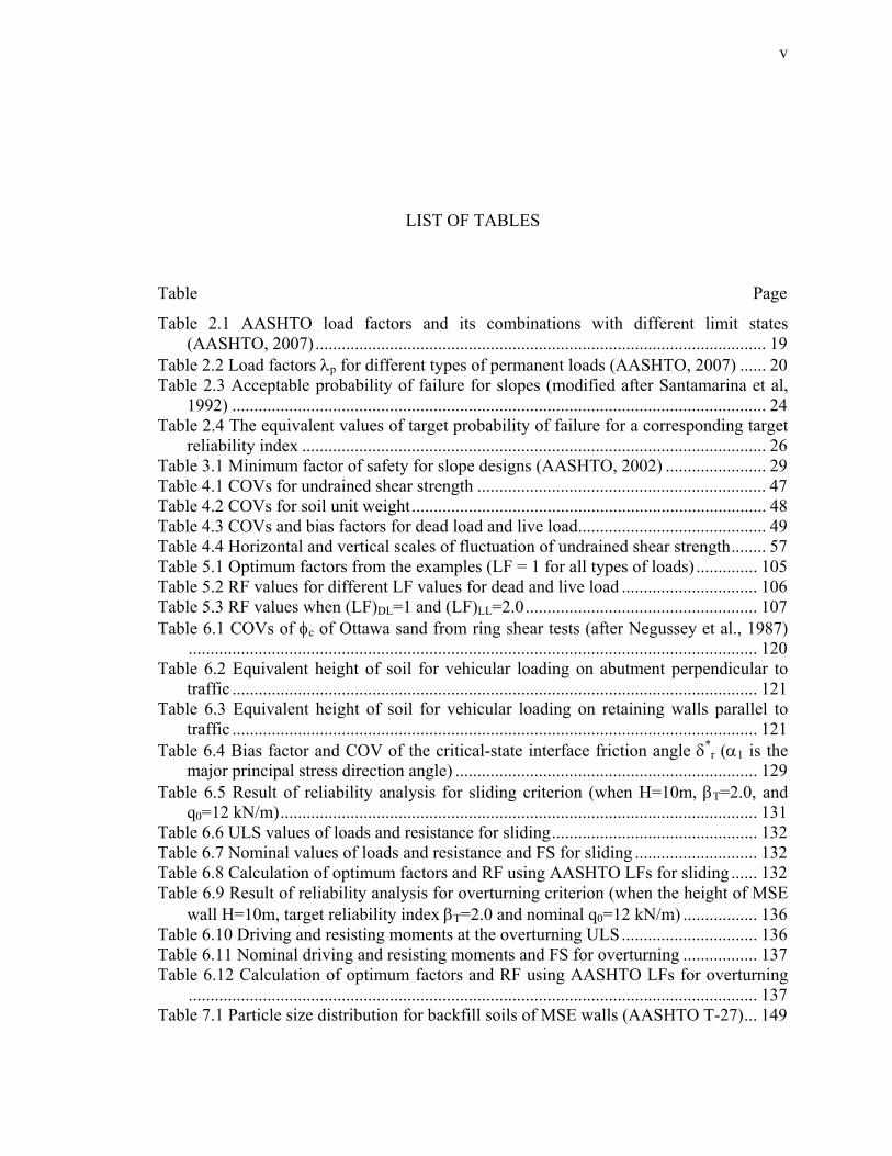
LIST OF TABLES
Table Page
Table 2.1 AASHTO load factors and its combinations with different limit states (AASHTO, 2007) ....................................................................................................... 19
Table 2.2 Load factors λp for different types of permanent loads (AASHTO, 2007) ...... 20 Table 2.3 Acceptable probability of failure for slopes (modified after Santamarina et al,
1992) .......................................................................................................................... 24 Table 2.4 The equivalent values of target probability of failure for a corresponding target
reliability index .......................................................................................................... 26 Table 3.1 Minimum factor of safety for slope designs (AASHTO, 2002) ....................... 29 Table 4.1 COVs for undrained shear strength .................................................................. 47 Table 4.2 COVs for soil unit weight ................................................................................. 48 Table 4.3 COVs and bias factors for dead load and live load ........................................... 49 Table 4.4 Horizontal and vertical scales of fluctuation of undrained shear strength ........ 57 Table 5.1 Optimum factors from the examples (LF = 1 for all types of loads) .............. 105 Table 5.2 RF values for different LF values for dead and live load ............................... 106 Table 5.3 RF values when (LF)DL=1 and (LF)LL=2.0 ..................................................... 107 Table 6.1 COVs of φc of Ottawa sand from ring shear tests (after Negussey et al., 1987)
.................................................................................................................................. 120 Table 6.2 Equivalent height of soil for vehicular loading on abutment perpendicular to
traffic ........................................................................................................................ 121 Table 6.3 Equivalent height of soil for vehicular loading on retaining walls parallel to
traffic ........................................................................................................................ 121 Table 6.4 Bias factor and COV of the critical-state interface friction angle δ*
r (α1 is the major principal stress direction angle) ..................................................................... 129
Table 6.5 Result of reliability analysis for sliding criterion (when H=10m, βT=2.0, and q0=12 kN/m) ............................................................................................................. 131
Table 6.6 ULS values of loads and resistance for sliding ............................................... 132 Table 6.7 Nominal values of loads and resistance and FS for sliding ............................ 132 Table 6.8 Calculation of optimum factors and RF using AASHTO LFs for sliding ...... 132 Table 6.9 Result of reliability analysis for overturning criterion (when the height of MSE
wall H=10m, target reliability index βT=2.0 and nominal q0=12 kN/m) ................. 136 Table 6.10 Driving and resisting moments at the overturning ULS ............................... 136 Table 6.11 Nominal driving and resisting moments and FS for overturning ................. 137 Table 6.12 Calculation of optimum factors and RF using AASHTO LFs for overturning
.................................................................................................................................. 137 Table 7.1 Particle size distribution for backfill soils of MSE walls (AASHTO T-27) ... 149

vi
Table 7.2 γdmax measured using ASTM D4253 ............................................................... 150 Table 7.3 γdmin measured using ASTM D4254 ............................................................... 151 Table 7.4 COVs of relative density of compacted fine sand .......................................... 154 Table 7.5 COVs of relative density of compacted gravelly sand ................................... 154 Table 7.6 Result of reliability analysis for pullout of steel-strip reinforcement (when
sv=0.6m, sh=0.75m, z=0.60m, H=20m, βT=3.0, and the nominal q0=12 kN/m) ...... 173 Table 7.7 ULS values of loads and resistance for pullout of steel-strip reinforcement .. 174 Table 7.8 Nominal values of loads and resistance and FS value for pullout of steel-strip
reinforcement ........................................................................................................... 174 Table 7.9 Calculation of optimum factors and RF using AASHTO LFs for pullout of
steel-strip reinforcement ........................................................................................... 175 Table 7.10 Result of reliability analysis for structural failure of steel-strip reinforcement
(sv=0.8m, sh=0.75m and βT=3.5) .............................................................................. 187 Table 7.11 ULS values of loads and resistance for structural failure of steel-strip
reinforcement ........................................................................................................... 187 Table 7.12 Nominal values of loads and resistance and FS value for structural failure of
steel-strip reinforcement ........................................................................................... 188 Table 7.13 Calculation of optimum factors and RF using AASHTO LFs for structural
failure of steel-strip reinforcement ........................................................................... 188 Table 7.14 RF and the corresponding reinforcement level for different target reliability
indices (sh = 0.75m) .................................................................................................. 189 Table 7.15 FS for different target reliability indices (sh = 0.75m) .................................. 189 Table 8.1 RF value for structural failure of steel-strip reinforcement for γrf = 20 and 22
kN/m3 (when live surcharge load q0 = 12kN/m) ...................................................... 202 Table 8.2 RF values for sliding criterion ........................................................................ 207 Table 8.3 RF values for overturning criterion ................................................................ 207 Table 8.4 Minimum RF value for pullout of steel-strip reinforcement for 5m-high MSE
wall (with q0=14 kN/m) ........................................................................................... 208 Table 8.5 Minimum RF value for pullout of steel-strip reinforcement for MSE walls more
than 6m-tall (with q0=12 kN/m) ............................................................................... 208 Table 8.6 RF value for structural failure of steel-strip reinforcement ............................ 208

vii
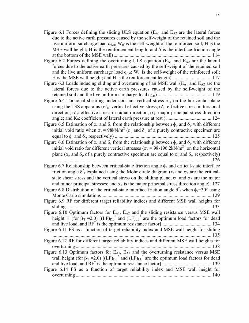
LIST OF FIGURES
Figure Page
Figure 2.1 Distribution of total load Q and resistance R when two different cases have the same value of FS: (a) high load and resistance uncertainty and (b) low load and resistance uncertainty ................................................................................................. 15
Figure 2.2 Normal distribution of margin of safety G (μG and σG are the mean and standard deviation of margin of safety G, and β is reliability index) ......................... 22
Figure 3.1 Method of slices (li is the length of the bottom of ith slice; i=1,···,n) .............. 31 Figure 3.2 Free-body diagram of ith slice .......................................................................... 32 Figure 3.3 Algorithm for LRFD of slopes ........................................................................ 35 Figure 3.4 Geometry and soil parameters of the slope .................................................... 36 Figure 3.5 The array of data points generated by Gaussian random field theory ............ 37 Figure 3.6 Finding the most critical slip surface among a large number of trial slip
surfaces ....................................................................................................................... 38 Figure 4.1 Four sources of uncertainty in soil property measurement (after Christian et
al., 1994) ..................................................................................................................... 40 Figure 4.2 Scatter of the in situ values of a soil property. ............................................... 42 Figure 4.3 Bias due to statistical error in the mean.......................................................... 43 Figure 4.4 Bias due to measurement procedures ............................................................. 44 Figure 4.5 Measurement error ........................................................................................... 45 Figure 4.6 Live loads considered in slope design (consider destabilizing live surcharges
and neglect stabilizing live surcharges) ..................................................................... 49 Figure 4.7 Exponential correlation coefficient functions for different isotropic scales of
fluctuation (in one-direction) (sf is the scale of fluctuation) ...................................... 53 Figure 4.8 Surface maps of the exponential correlation coefficient functions in 2D space
for different isotropic scales of fluctuation; (a) sf =1m, (b) sf =5m, (c) sf =10m, and (d) sf =20m ................................................................................................................. 54
Figure 4.9 Meaning of scale of fluctuation sf for the exponential correlation coefficient function in 1D space ................................................................................................... 58
Figure 4.10 Estimation of the variance of measurement error of undrained shear strength su by comparing the autocovariance function with the measured autocovariance values of undrained shear strength (after Christian et al., 1994) ............................... 64
Figure 4.11 Horizontal and tilted views of surface map of two-dimensional Gaussian random fields that has zero mean and unit standard deviation for different scales of fluctuation; (a) sf = 1m, (b) sf = 5m, (c) sf = 10m, and (d) sf = 20m .......................... 71
Figure 5.1 Geometry of a three-layer soil slope and its soil properties ............................ 73

viii
Figure 5.2 Effect of the COV of measurement on a probability of failure of the slope given in Figure 5.1 ..................................................................................................... 74
Figure 5.3 Probability of failure of the slope shown in Figure 5.1 for different isotropic scale of fluctuation of soil unit weight ....................................................................... 75
Figure 5.4 Effect of the isotropic scale of fluctuation on a probability of failure ............ 76 Figure 5.5 Geometry of a three-layer soil slope ............................................................... 78 Figure 5.6 Distribution of FS value and the ULS of the slope (Pf = 0.001 and without live
uniform surcharge load) ............................................................................................. 79 Figure 5.7 Distribution of optimum load factor (LF)*
DL for load due to self-weight of soil .................................................................................................................................... 81
Figure 5.8 Distribution of optimum resistance factor RF* ................................................ 82 Figure 5.9 Distribution of FS value and the ULS of the slope (Pf = 0.01, no live uniform
surcharge load) ........................................................................................................... 84 Figure 5.10 Distribution of optimum load factor (LF)*
LD for load due to self-weight of soil .............................................................................................................................. 85
Figure 5.11 Distribution of optimum resistance factor RF* .............................................. 86 Figure 5.12 Distribution of FS value and the ULS of the slope (Pf = 0.001 and live
uniform surcharge load q0 = 12 kN/m) ...................................................................... 87 Figure 5.13 Distribution of optimum load factor (LF)*
DL for load due to self-weight of soil .............................................................................................................................. 89
Figure 5.14 Distribution of optimum load factor (LF)*LL for load due to live surcharge
load ............................................................................................................................. 90 Figure 5.15 Distribution of optimum resistance factor RF* .............................................. 91 Figure 5.16 Distribution of FS value and the ULS of the slope (Pf = 0.01 and live uniform
surcharge load q0 = 12 kN/m) .................................................................................... 92 Figure 5.17 Distribution of optimum load factor (LF)*
DL for load due to self-weight of soil .............................................................................................................................. 94
Figure 5.18 Distribution of optimum load factor (LF)*LL for load due to live surcharge
load ............................................................................................................................. 94 Figure 5.19 Distribution of optimum resistance factor RF* .............................................. 95 Figure 5.20 Geometry of a road embankment (1:1 side slopes) ....................................... 96 Figure 5.21 Distribution of FS value and the ULS of the slope (Pf = 0.001 and live
uniform surcharge load q0 = 12 kN/m) ...................................................................... 97 Figure 5.22 Distribution of optimum load factor (LF)*
DL for load due to self-weight of soil .............................................................................................................................. 99
Figure 5.23 Distribution of optimum load factor (LF)*LL for load due to live surcharge
load ............................................................................................................................. 99 Figure 5.24 Distribution of optimum resistance factor RF* ............................................ 100 Figure 5.25 Distribution of FS value and the ULS of the slope (Pf = 0.01 and live uniform
surcharge load q0 = 12 kN/m) .................................................................................. 101 Figure 5.26 Distribution of optimum load factor (LF)*
DL for load due to self-weight of soil ............................................................................................................................ 103
Figure 5.27 Distribution of optimum load factor (LF)*LL for load due to live surcharge
load ........................................................................................................................... 103 Figure 5.28 Distribution of optimum resistance factor RF* ............................................ 104
ix
Figure 6.1 Forces defining the sliding ULS equation (EA1 and EA2 are the lateral forces due to the active earth pressures caused by the self-weight of the retained soil and the live uniform surcharge load q0,rt; Wrf is the self-weight of the reinforced soil; H is the MSE wall height; H is the reinforcement length; and δ is the interface friction angle at the bottom of the MSE wall) ................................................................................ 114
Figure 6.2 Forces defining the overturning ULS equation (EA1 and EA2 are the lateral forces due to the active earth pressures caused by the self-weight of the retained soil and the live uniform surcharge load q0,rt; Wrf is the self-weight of the reinforced soil; H is the MSE wall height; and H is the reinforcement length) ................................ 117
Figure 6.3 Loads inducing sliding and overturning of an MSE wall (EA1 and EA2 are the lateral forces due to the active earth pressures caused by the self-weight of the retained soil and the live uniform surcharge load q0,rt) ............................................ 119
Figure 6.4 Torsional shearing under constant vertical stress σ′a on the horizontal plane using the TSS apparatus (σ′a: vertical effective stress; σ′t: effective stress in torsional direction; σ′r: effective stress in radial direction; α1: major principal stress direction angle; and K0: coefficient of lateral earth pressure at rest ) ..................................... 124
Figure 6.5 Estimation of φc and δr from the relationship between φp and δp with different initial void ratio when σa = 98kN/m2 (φp and δp of a purely contractive specimen are equal to φc and δr, respectively) ............................................................................... 125
Figure 6.6 Estimation of φc and δr from the relationship between φp and δp with different initial void ratio for different vertical stresses (σa = 98-196.2kN/m2) on the horizontal plane (φp and δp of a purely contractive specimen are equal to φc and δr, respectively) .................................................................................................................................. 126
Figure 6.7 Relationship between critical-state friction angle φc and critical-state interface friction angle δ*
r explained using the Mohr circle diagram (τr and σa are the critical-state shear stress and the vertical stress on the sliding plane; σ1 and σ3 are the major and minor principal stresses; and α1 is the major principal stress direction angle) . 127
Figure 6.8 Distribution of the critical-state interface friction angle δ*r when φc=30° using
Monte Carlo simulations .......................................................................................... 129 Figure 6.9 RF for different target reliability indices and different MSE wall heights for
sliding ....................................................................................................................... 133 Figure 6.10 Optimum factors for EA1, EA2 and the sliding resistance versus MSE wall
height H (for βT =2.0) [(LF)DL* and (LF)LL
* are the optimum load factors for dead and live load, and RF* is the optimum resistance factor] ......................................... 134
Figure 6.11 FS as a function of target reliability index and MSE wall height for sliding .................................................................................................................................. 135
Figure 6.12 RF for different target reliability indices and different MSE wall heights for overturning ............................................................................................................... 138
Figure 6.13 Optimum factors for EA1, EA2 and the overturning resistance versus MSE wall height (for βT =2.0) [(LF)DL
* and (LF)LL* are the optimum load factors for dead
and live load, and RF* is the optimum resistance factor] ......................................... 139 Figure 6.14 FS as a function of target reliability index and MSE wall height for
overturning ............................................................................................................... 140

x
Figure 7.1 Loads for pullout and structural failure of the steel-strip reinforcement (Fr,DL and Fr,LL are the lateral loads acting on the reinforcement due to the self-weight of the reinforced soil and due to the live uniform surcharge load on the top of the reinforced soil q0,rf) .................................................................................................................... 145
Figure 7.2 Location of maximum tensile forces on the reinforcements and distribution of tensile force along the reinforcements ..................................................................... 146
Figure 7.3 Location of the maximum tensile force normalized by the height of MSE walls .................................................................................................................................. 148
Figure 7.4 Relationship between relative density and relative compaction .................... 152 Figure 7.5 Particle size distributions of fine sand and gravelly sand introduced in ASTM
D2049-69 .................................................................................................................. 153 Figure 7.6 Variation of Kr/ KA for MSE walls with steel-strip reinforcements (φ′ is peak
friction angle; after Schlosser, 1978) ....................................................................... 156 Figure 7.7 Relationship between K0 and e0 of Minnesota sand ...................................... 158 Figure 7.8 Coefficient of lateral earth pressure at rest for normally consolidated Toyoura
sand when axial stress is 118 kPa ............................................................................ 159 Figure 7.9 Coefficient of lateral earth pressure at rest for normally consolidated Toyoura
sand when axial stress is 196 kPa ............................................................................ 159 Figure 7.10 Distribution of Kr with depth z from the top of an MSE wall using the
modified coherent gravity method ........................................................................... 161 Figure 7.11 Relationship between the measured and predicted maximum tensile forces
based on the modified coherent gravity method ...................................................... 163 Figure 7.12 Ratio of measured to predicted Tmax with depth from the top of MSE walls
(average value=0.666) .............................................................................................. 164 Figure 7.13 Relationship between predicted Tmax multiplied by bias factor and measured
Tmax based on the modified coherent gravity method .............................................. 165 Figure 7.14 Residuals of Kr estimation with depth from the top of MSE walls ............. 165 Figure 7.15 Result of the regression analysis of Kr on z with zcr = 6m and φc = 33° ...... 167 Figure 7.16 Result of the regression analysis of Kr on zcr = 4.2m, φc = 35.7° and z ....... 167 Figure 7.17 Comparison between CR suggested by AASHTO and FHWA specifications
and CR data point from pullout tests (Data points from Commentary of the 1994 AASHTO Standard Specifications for Highway Bridges) ....................................... 169
Figure 7.18 Distribution of yield strength of steel-strip reinforcements (data acquired from the Reinforced Earth Company) ...................................................................... 171
Figure 7.19 RF for pullout of steel-strip reinforcement versus reinforcement depth z when sh=0.375m and sv=0.3m ........................................................................................... 176
Figure 7.20 RF for pullout of steel-strip reinforcement versus reinforcement depth z when sh=0.75m and sv=0.3m ............................................................................................. 176
Figure 7.21 RF for pullout of steel-strip reinforcement versus reinforcement depth z when sh=0.375m and sv=0.6m ........................................................................................... 177
Figure 7.22 RF for pullout of steel-strip reinforcement versus reinforcement depth z when sh=0.75m and sv=0.6m ............................................................................................. 177
Figure 7.23 RF for pullout of steel-strip reinforcement versus reinforcement depth z when sh=0.375m and sv=0.8m ........................................................................................... 178

xi
Figure 7.24 RF for pullout of steel-strip reinforcement versus reinforcement depth z when sh=0.75m and sv=0.8m ............................................................................................. 178
Figure 7.25 Changes of optimum factors (resistance factor, load factors for live load and dead load) with an increasing reinforcement depth from the top of MSE wall (sv=0.60m, H=20m, βT=3.0, and q0=12 kN/m) [(LF)DL
* and (LF)LL* are the optimum
load factors for dead and live load, and RF* is the optimum resistance factor] ....... 179 Figure 7.26 Changes of RF*, (LF)DL
*/(LF)DL, and (LF)LL*/(LF)LL with increasing
reinforcement depth z (sv=0.60m, H=20m, βT=3.0, and q0=12 kN/m) [(LF)DL* and
(LF)LL* are the optimum load factors for dead and live load, RF* is the optimum
resistance factor, and (LF)DL and (LF)LL are the AASHTO load factors] ................ 181 Figure 7.27 FS for pullout of steel-strip reinforcement versus reinforcement depth z when
sh=0.375m and sv=0.3m ........................................................................................... 182 Figure 7.28 FS for pullout of steel-strip reinforcement versus reinforcement depth z when
sh=0.75m and sv=0.3m ............................................................................................. 182 Figure 7.29 FS for pullout of steel-strip reinforcement versus reinforcement depth z when
sh=0.375m and sv=0.6m ........................................................................................... 183 Figure 7.30 FS for pullout of steel-strip reinforcement versus reinforcement depth z when
sh=0.75m and sv=0.6m ............................................................................................. 183 Figure 7.31 FS for pullout of steel-strip reinforcement versus reinforcement depth z when
sh=0.375m and sv=0.8m ........................................................................................... 184 Figure 7.32 FS for pullout of steel-strip reinforcement versus reinforcement depth z when
sh=0.75m and sv=0.8m ............................................................................................. 184 Figure 7.33 Reliability index β for structural failure of steel-strip reinforcement versus
reinforcement depth z (horizontal reinforcement spacing sh = 0.75m and vertical reinforcement spacing sv = 0.4, 0.5, 0.6, 0.7, and 0.8m) .......................................... 186
Figure 8.1 RF for sliding for different MSE wall heights when φc,rt is equal to 30° and 33° (q0 is the live surcharge load) ................................................................................... 191
Figure 8.2 RF for overturning for different MSE wall heights when φc,rt is equal to 30° and 33° (q0 is the live surcharge load) ..................................................................... 192
Figure 8.3 Minimum RF for pullout of steel-strip reinforcement for different values of DR,rf when sv=0.3m (q0 is the live surcharge load) ................................................... 193
Figure 8.4 Minimum RF for pullout of steel-strip reinforcement for different values of DR,rf when sv=0.6m (q0 is the live surcharge load) ................................................... 194
Figure 8.5 Minimum RF for pullout of steel-strip reinforcement for different values of DR,rf when sv=0.8m (q0 is the live surcharge load) ................................................... 194
Figure 8.6 Minimum RF for pullout of steel-strip reinforcement for different values of δcv when sv=0.3m (q0 is the live surcharge load) ........................................................... 195
Figure 8.7 Minimum RF for pullout of steel-strip reinforcement for different values of δcv when sv=0.6m (q0 is the live surcharge load) ........................................................... 196
Figure 8.8 Minimum RF for pullout of steel-strip reinforcement for different values of δcv when sv=0.8m (q0 is the live surcharge load) ........................................................... 196
Figure 8.9 RF for sliding for different MSE wall heights when γrt = 18 and 20 kN/m3 (q0 is the live surcharge load) ........................................................................................ 197
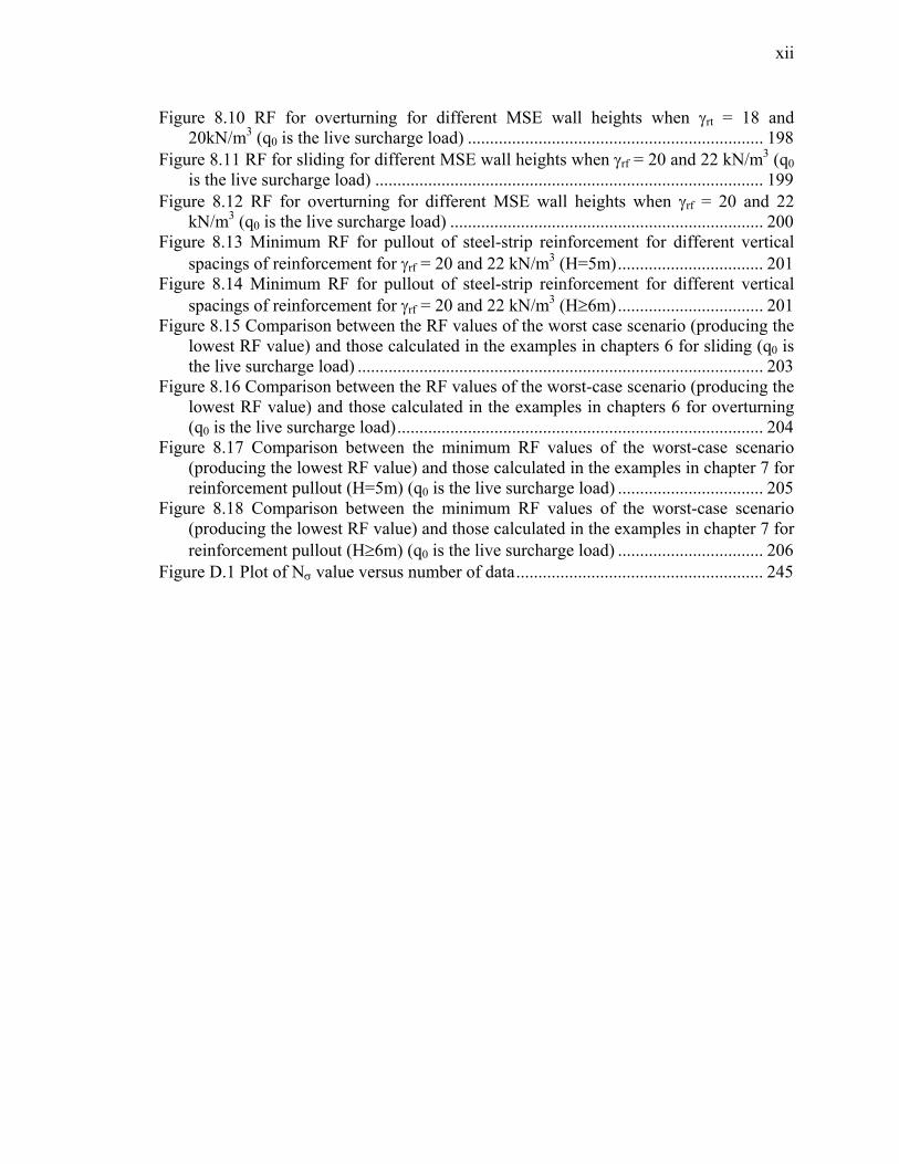
xii
Figure 8.10 RF for overturning for different MSE wall heights when γrt = 18 and 20kN/m3 (q0 is the live surcharge load) ................................................................... 198
Figure 8.11 RF for sliding for different MSE wall heights when γrf = 20 and 22 kN/m3 (q0 is the live surcharge load) ........................................................................................ 199
Figure 8.12 RF for overturning for different MSE wall heights when γrf = 20 and 22 kN/m3 (q0 is the live surcharge load) ....................................................................... 200
Figure 8.13 Minimum RF for pullout of steel-strip reinforcement for different vertical spacings of reinforcement for γrf = 20 and 22 kN/m3 (H=5m) ................................. 201
Figure 8.14 Minimum RF for pullout of steel-strip reinforcement for different vertical spacings of reinforcement for γrf = 20 and 22 kN/m3 (H≥6m) ................................. 201
Figure 8.15 Comparison between the RF values of the worst case scenario (producing the lowest RF value) and those calculated in the examples in chapters 6 for sliding (q0 is the live surcharge load) ............................................................................................ 203
Figure 8.16 Comparison between the RF values of the worst-case scenario (producing the lowest RF value) and those calculated in the examples in chapters 6 for overturning (q0 is the live surcharge load) ................................................................................... 204
Figure 8.17 Comparison between the minimum RF values of the worst-case scenario (producing the lowest RF value) and those calculated in the examples in chapter 7 for reinforcement pullout (H=5m) (q0 is the live surcharge load) ................................. 205
Figure 8.18 Comparison between the minimum RF values of the worst-case scenario (producing the lowest RF value) and those calculated in the examples in chapter 7 for reinforcement pullout (H≥6m) (q0 is the live surcharge load) ................................. 206
Figure D.1 Plot of Nσ value versus number of data ........................................................ 245

1
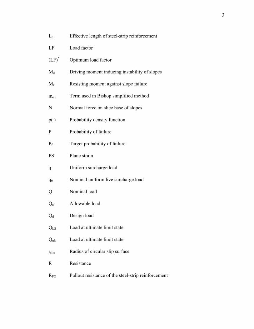
LIST OF SYMBOLS
Ac Cross-sectional area of steel-strip reinforcement
Amn Fourier coefficient
b Width of steel-strip reinforcements or slices of slopes
Bmn Fourier coefficient
BSM Bishop simplified method
BST Borehole shear test
c Apparent cohesion
COV Coefficient of variation
Cov Covariance
CR Pullout resistance factor
D10 Diameter corresponding to weight-percent of soil finer than 10%
D50 Diameter corresponding to weight-percent of soil finer than 50%
D60 Diameter corresponding to weight-percent of soil finer than 60%
DR Relative density
DST Direct shear test
EA1 Lateral forces due to the active earth pressures by the self-weight of the retained soil
EA2 Lateral forces due to the active earth pressures by live uniform surcharge load

2
e Measurement error
emax Maximum void ratio
emin Minimum void ratio
FORM First-Order Reliability Method
FS Factor of safety
fy Yield strength of steel-strip reinforcement
Fr,DL Lateral load acting on the reinforcement due to self-weight of reinforced soil
Fr,LL Lateral load acting on the reinforcement due to live uniform surcharge load on the top of reinforced soil
G Margin of safety
G( ) Spectral density function
Gs Specific gravity of soil
H Height of an MSE wall
heq Equivalent height of soil for vehicular loading
K1 Finite number of discretization in x uni-direction
K2 Finite number of discretization in y uni-direction
KA Active earth pressure coefficient
Kr Coefficient of lateral earth pressure
L Total length of steel-strip reinforcement
L1 Length of Gaussian random field in horizontal direction
L2 Length of Gaussian random field in vertical direction
La Steel-strip reinforcement length inside active zone in reinforced soil
3
Le Effective length of steel-strip reinforcement
LF Load factor
(LF)* Optimum load factor
Md Driving moment inducing instability of slopes
Mr Resisting moment against slope failure
mα,i Term used in Bishop simplified method
N Normal force on slice base of slopes
p( ) Probability density function
P Probability of failure
Pf Target probability of failure
PS Plane strain
q Uniform surcharge load
q0 Nominal uniform live surcharge load
Q Nominal load
Qa Allowable load
Qd Design load
QLS Load at ultimate limit state
Qult Load at ultimate limit state
rslip Radius of circular slip surface
R Resistance
RPO Pullout resistance of the steel-strip reinforcement

4
RF Resistance factor
(RF)* Optimum resistance factor
RLS Resistance at ultimate limit state
Rn Nominal resistance
s Separation distance
sf Scale of fluctuation
sf,iso Isotropic scale of fluctuation
sf,x Scale of fluctuation in the horizontal direction
sf,y Scale of fluctuation in the vertical direction
sh Horizontal spacing of steel-strip reinforcement
sv Vertical spacing of steel-strip reinforcement
su Undrained shear strength
T Tangential force on slice base
Tmax Maximum tensile force on steel-strip reinforcement
U Water force on slice base
VST Vane shear test
W Weight of soil (slice)
WSD Working Stress Design
X Horizontal component of inter-slice forces of a slice
Y Vertical component of inter-slice forces of a slice
Z Standard normal random variable

5
zcr Depth from the top of an MSE wall where active condition prevails
zm Measurement of soil property
zspat Soil property value reflecting spatial variability
Φ( ) Standard normal cumulative distribution function
α Inclination angle to the horizontal plane of slice base
pδα Bias factor of interface friction angle between backfill material in reinforced soil and steel-strip reinforcement
α1 Major principal stress direction angle
β Reliability index
βT Target reliability index
δcv Critical-state interface friction angle
δp Interface friction angle between backfill material in reinforced soil and steel-strip reinforcement
δ* Interface friction angle at the bottom of an MSE wall
δ*p Peak interface friction angle at the bottom of an MSE wall
δ*r Critical-state interface friction angle at the bottom of an MSE wall
φ Friction angle
φc Critical-state friction angle
φp Peak friction angle
γ Shear strain (or unit weight of soil)
γd Dry unit weight of soil
γdmax Maximum dry unit weight of soil
γdmin Minimum dry unit weight of soil

6
pδη Distributor parameter for interface friction angle between backfill material in reinforced soil and steel-strip reinforcement
λ Mean of the lognormal distribution
λp Load factors for different type of permanent loads
μ Mean
μbias Mean accounting bias due to measurement procedure
μG Mean of margin of safety
μmeas Mean accounting measurement error
μR Mean of resistance
μreal Mean of real in-situ values
μQ Mean of load
μstat Mean accounting statistical error
ρ( ) Correlation coefficient function
σG Standard deviation of margin of safety
σ Standard deviation
σ1 Major principal stress
σ3 Minor principal stress
σa Constant vertical stress
σR Standard deviation of resistance
σQ Standard deviation of load
σv Vertical stress
σ′h Horizontal effective stress
7
σ′v Vertical effective stress
τ Shear stress
τr Residual shear stress
ωx Angular frequency for x direction
ωy Angular frequency for y direction
ζ Standard deviation of the lognormal distribution

8
PART I – INTRODUCTORY CONCEPTS
9
CHAPTER 1. INTRODUCTION
1.1. Introduction
The primary goal of this report was to develop Load and Resistance Factor Design
(LRFD) methods for slope and retaining structure design. Even though there is past
research on LRFD of shallow foundations and piles, there are few publications available
on LRFD of slopes and retaining structures (notable among these being Chen, 1999;
Chen, 2000; Simpson, 1992; Loehr et al, 2005). The design goals for slopes and retaining
structures are the economical selection of the slope angle and slope protection measures
(in the case of slopes) and the type and appropriate dimensions (in the case of retaining
walls) in order to avoid “failure.”
The design of slopes and retaining structures has traditionally been conducted
using the Working Stress Design (WSD) approach. Even in recent years, it remains the
primary design approach in geotechnical engineering. Within this framework, every
design problem becomes one of comparing a capacity or resistance with a loading. To
account for the uncertainties, a single factor of safety is used to divide the capacity (or,
from the opposite point of view, to multiply the loading) before the comparison is made.
The factor of safety is the tool that the WSD approach uses to account for uncertainties.
The uncertainties are expressed in a single number, the factor of safety, so there is no way
in WSD to separate the uncertainties related to load estimation, for example, from those
related to soil variability.
The LRFD method combines the Limit States Design (LSD) concept with the
probabilistic approach that accounts for the uncertainty of parameters that are related to
both the loads and the resistance. There are two types of limit states (Salgado 2008): (1)
Ultimate Limit States (ULS) and (2) Serviceability Limit States (SLS). An ULS is related
to lack of safety of structures, such as structural failure or collapse, and serviceability

10
limit state is associated with malfunctioning of structures, such as excessive uniform or
differential settlement of structures. In this report, only ULSs are considered.
An ULS is a state for which the total load is equal to the maximum resistance of
the system. When the total load matches the maximum resistance of the system, the
system fails. To prevent failure of the system, LSD requires the engineer to identify every
possible ULS during design in order to make sure that it is not reached. However, in the
case of LRFD, which combines the probabilistic approach with LSD, the probability of
failure of the system is calculated from the probability density distributions of the total
load and the maximum resistance. Probability of failure for a given ULS is the
probability of attainment of that ULS. LRFD aims to keep this probability of failure from
exceeding a certain level (the target probability of failure or target reliability index).
Finally, LRFD is explained using an LSD framework, which checks for the ULS using
partial factors on loads and on resistance. These partial factors associated with the loads
and the resistance are calculated based on their uncertainties.
1.2. Problem Statement
There are issues that geotechnical engineers face when using LRFD in geotechnical
designs. Some of the main issues are:
1) As opposed to concrete or steel, which are manufactured materials and thus
have properties that assume values within a relatively narrow spread, soils are
materials deposited in nature in ways that lead them to have properties that show
striking spatial variability. In addition, soil exhibits anisotropic properties. The
result of this is that soil properties assume values that are widely dispersed around
an average; therefore, the assessment of the uncertainties of soil parameters is
very important for economical design.
2) It is usually true in structural design, and to a large extent in foundation design,
that load and resistance effects are reasonably independent; this is not true for
11
slopes and retaining structures, for which soil weight is both a significant source
of the loading and a significant source of the resistance to sliding. This has
created problems for engineers attempting to design such structures using LRFD,
leading to doubts about the approach.
3) Because of the wide variability in the shear strength of soils, the loosely
defined values of resistance factors in the codes and the lack of familiarity by
engineers with the LRFD approach, engineers have often been conservative when
using the LRFD approach in design (Becker, 1996). In this report, the equations
for loads and resistance reflect well established concepts, and the process of
calculating load factors and resistance factor is well explained for easy
understanding.
4) Different organizations in Europe, Canada, and the U.S. have proposed
different types of ULS factored design. In Europe it is customary to factor soil
shear strength (that is, c and φ) directly (Eurocode 7, 1994), while in North
America the codes and recommendations (e.g., AASHTO, 2007) propose to factor
the final soil resistance or shear strength (which creates certain difficulties). The
load factors vary widely across codes; in the U.S., for example, the load factors
recommended in the American Association of State Highway and Transportation
(AASHTO) LRFD bridge design specifications (2007) are not the same as those
recommended in the ACI reinforced concrete code. The resistance factors have
typically been defined through rough calibrations with the WSD approach. This
myriad of methods, recommendations, and values has led to considerable
confusion and has not made it easier for the practicing engineer to use the
approach. We intend to clarify such issues.
The LRFD approach in the case of slopes and retaining structures poses a
different but interesting challenge to geotechnical engineers. Unlike structural or
conventional geotechnical designs, both the load and resistance contain soil parameters

12
(Goble 1999). The weight of the soil is a source of both the demand (load) and the
capacity (resistance) in the case of slopes and retaining structures. This makes the
problem complicated since the load and resistance factors have to be extracted from the
same parameters.
The calculation of loads in the case of foundation problems is straightforward.
However, in the case of retaining structures, the loads come partly from dead load (earth
pressures due to self-weight of soil) and partly from live load (e.g., vehicular load on the
top of the retaining structures). It is important to determine which factors must be used
for each load source when calculating the factored load. This situation greatly magnifies
the advantage of LRFD over WSD. In WSD, a single factor (factor of safety) would be
used to account for the uncertainties, possibly leading to unnecessarily conservative
designs.
The interest in LRFD comes, ultimately, from the expectation that LRFD designs
are more economical than WSD designs for the same level of safety (in terms of
probability of failure of the structures). This economy would be a consequence of a
number of possibilities offered by the LRFD approach, but not by WSD, namely:
(1) To account for load uncertainties and resistance uncertainties separately, and
consequently, more realistically;
(2) To more precisely define a characteristic shear strength or characteristic soil
resistance;
(3) To allow separate consideration of permanent versus temporary or accidental
loads;
(4) To design following the same general approach followed by structural
engineers, eliminating the design interface currently in place and encouraging
better interaction between the geotechnical and the structural engineers;
(5) To allow future improvements in the design of geotechnical structures;
(6) To allow each type of analysis or design method to have its own resistance
factors.

13
1.3. Objectives
In order to realize the potential benefits (1) through (6) outlines in the previous section of
the LRFD approach, a credible set of load and resistance factors and a compatible way of
defining characteristic soil resistance that can be consistently used by geotechnical
engineers needs to be determined. This system must be based on more than rough
calibrations of LRFD with WSD, which is the basic procedure followed in the current
AASHTO LRFD bridge design specifications (2007). Load and resistance factors must
also be based on scientifically defensible methods. They must be based on analysis that
considers the underlying probabilistic nature of loads and resistances, on a reasonable
proposal of how to define characteristic shear strength and characteristic soil resistance,
and on the models and analyses that will be used to analyze the various slope and
retaining structure design problems.
This study focuses on the general analysis and design methods of both slopes and
MSE walls and provides examples of them. In order to accomplish these tasks, a number
of intermediate objectives need to be achieved:
(1) Determination of load factors from AASHTO LRFD specifications (2007) for
permanent and temporary loads of different types and under various
combinations;
(2) Determination of the best equation for each ULS to be checked;
(3) Development of recommendations on how to assess the uncertainty of soil
parameters;
(4) Development of resistance factors compatible with the load factors.
14
CHAPTER 2. LOAD AND RESISTANCE FACTOR DESIGN
2.1. Load and Resistance Factor Design Compared with Working Stress Design
As mentioned in the previous chapter, the concept of Working Stress Design (WSD) has
been commonly used in geotechnical analyses and designs for many decades.
Appropriate values of Factor of Safety (FS) were suggested for most of the geotechnical
structures, such as shallow foundations, piles, slopes, embankments, and retaining
structures, and those values have been determined based on accumulated experience from
case histories and failure data. However, using a single FS in design is not the best choice
in the sense that the method does not consider the uncertainty of the loads applied on the
structure and the resistance of the structure separately. In Figure 2.1, due to higher
uncertainties of both the load and the resistance, the probability of failure of case (a) is
much higher than that of case (b) although the values of FS in both cases are the same.

15
Probability density
Load Q, Resistance R
Load QResistance R
Load Q, Resistance R
Load QR esistance R
Probability density(a)
(b)
Figure 2.1 Distribution of total load Q and resistance R when two different cases have the same value of FS: (a) high load and resistance uncertainty and (b) low load and resistance
uncertainty
LRFD is a more sophisticated design method that considers the uncertainties of
load and resistance separately. LRFD in structural engineering has been successfully
adopted in practice. The design method has reduced costs for many types of steel and
concrete structures. The recent interest in the implementation of LRFD in geotechnical
engineering is due to the possibilities that it offers for a more rational and economical
design of foundations and geotechnical structures.
The FS is defined as the ratio of the ultimate resistance of an element to the total
load applied to the element. WSD imposes an extra margin of safety to the structure so
that it can withstand more load than the design (nominal) load. In WSD, the design load
is equal to or less than the allowable load, which is the load at ultimate limit state (ULS)
divided by FS:

16
ultd a
QQ QFS
≤ = (2.1)
where Qd is the design load, Qa is the allowable load, and Qult is the load at ULS.
As mentioned in the previous chapter, LRFD is based on the limit state design
framework, which compares the factored resistance to the sum of the factored loads. The
factors that are multiplied to the resistance and loads are determined based on the results
of reliability analyses and load factors (LFs) from design specifications, such as
AASHTO (2007), AISC (2005), and others. The method to determine these factors is
explained in the next section. According to LRFD, the following criterion needs to be
satisfied:
n i i(RF) R (LF) Q≥ ∑ (2.2)
where RF is the resistance factor, Rn is the nominal resistance, (LF)i are the load factors
that have different values for different types of loads and their combinations, and Qi are
the loads of various types, such as dead load, live load, earthquake load, and other
loading types.
2.2. Calculation of Resistance Factor RF
Calculation of the Resistance Factor (RF) in the inequality (2.2) is our final goal
in this study. The process of determining RF starts from the ULS equation. The ULS is
defined as the state at which the value of the total load is equal to that of the resistance:
LS i,LSR Q= ∑ (2.3)

17
We can rewrite Eq. (2.3) as
i,LSLSn i
n i
QR R QR Q
⎛ ⎞ ⎛ ⎞=⎜ ⎟ ⎜ ⎟
⎝ ⎠ ⎝ ⎠∑ (2.4)
We can define the optimum resistance factor (RF)* and the optimum load factors
(LF)i* as:
( )* LS
n
RRFR
= (2.5)
( )* i,LSi
i
QLF
Q= (2.6)
(RF)* and (LF)i* can be considered as the ideal resistance factor and load factors
that optimally satisfy inequality (2.2), but these optimum factors are problem-specific
(i.e., their values vary with input loads, geometry, and material parameters). For practical
purposes, design specifications provide fixed sets of load factors. Further modification of
Eq. (2.4) is necessary for calculating an RF value corresponding to predefined (virtually
always not optimal) load factors (LF)i.
Inequality (2.2) can be written as a design requirement as
( ) ( )* *
n iiRF R LF Q≥ ∑ (2.7)
and modified using a code-specified (LF)i:
( ) ( ) ( )( )
** i
n iii
LFRF R LF Q
LF
⎛ ⎞⎜ ⎟≥⎜ ⎟⎝ ⎠
∑ (2.8)
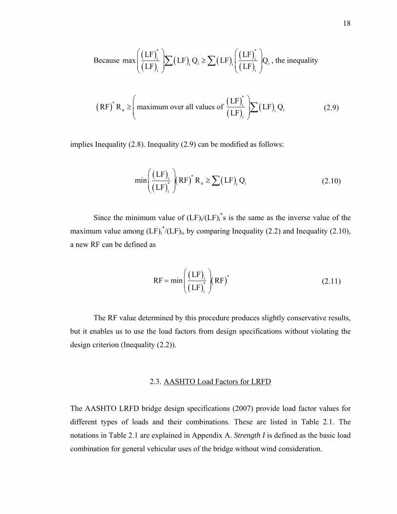
18
Because ( )( ) ( ) ( ) ( )
( )
* *
i ii ii i
i i
LF LFmax LF Q LF Q
LF LF
⎛ ⎞ ⎛ ⎞⎜ ⎟ ⎜ ⎟≥⎜ ⎟ ⎜ ⎟⎝ ⎠ ⎝ ⎠
∑ ∑ , the inequality
( ) ( )( ) ( )
** i
n iii
LFRF R maximum over all values of LF Q
LF
⎛ ⎞⎜ ⎟≥⎜ ⎟⎝ ⎠
∑ (2.9)
implies Inequality (2.8). Inequality (2.9) can be modified as follows:
( )( )
( ) ( )*in i* i
i
LFmin RF R LF Q
LF
⎛ ⎞⎜ ⎟ ≥⎜ ⎟⎝ ⎠
∑ (2.10)
Since the minimum value of (LF)i/(LF)i*s is the same as the inverse value of the
maximum value among (LF)i*/(LF)i, by comparing Inequality (2.2) and Inequality (2.10),
a new RF can be defined as
( )( )
( )*i*
i
LFRF min RF
LF
⎛ ⎞⎜ ⎟=⎜ ⎟⎝ ⎠
(2.11)
The RF value determined by this procedure produces slightly conservative results,
but it enables us to use the load factors from design specifications without violating the
design criterion (Inequality (2.2)).
2.3. AASHTO Load Factors for LRFD
The AASHTO LRFD bridge design specifications (2007) provide load factor values for
different types of loads and their combinations. These are listed in Table 2.1. The
notations in Table 2.1 are explained in Appendix A. Strength I is defined as the basic load
combination for general vehicular uses of the bridge without wind consideration.

19
Table 2.1 AASHTO load factors and its combinations with different limit states (AASHTO, 2007)
Load combination Limit state
DC DD DW EH EV ES EL
LL IM CE BR PL LS WA WS WL FR
TU CR SH TG SE
Use one of these at a time
EQ IC CT CVSTRENGTH І (unless noted) λp 1.75 1.00 − − 1.00 0.50/1.20 λTG λSE − − − −
STRENGTH ІІ λp 1.35 1.00 − − 1.00 0.50/1.20 λTG λSE − − − − STRENGTH ІІІ λp − 1.00 1.40 − 1.00 0.50/1.20 λTG λSE − − − − STRENGTH ІV λp − 1.00 − − 1.00 0.50/1.20 − − − − − − STRENGTH V λp 1.35 1.00 0.40 1.0 1.00 0.50/1.20 λTG λSE − − − − EXTREME EVENT І λp λEQ 1.00 − − 1.00 − − − 1.00 − − −
EXTREME EVENT ІІ λp 0.50 1.00 − − 1.00 − − − − 1.00 1.00 1.00
SERVICE І 1.00 1.00 1.00 0.30 1.0 1.00 1.00/1.20 λTG λSE − − − − SERVICE ІІ 1.00 1.30 1.00 − − 1.00 1.00/1.20 − − − − − − SERVICE ІІІ 1.00 0.80 1.00 − − 1.00 1.00/1.20 λTG λSE − − − − SERVICE ІV 1.00 − 1.00 0.70 − 1.00 1.00/1.20 − 1.00 − − − − FATIGUE -LL,IM & CE only − 0.75 − − − − − − − − − − −
(λp: load factors for different types of permanent loads, DC: dead load of structural components and nonstructural attachment, EH: horizontal earth pressure load, EV: vertical pressure from dead load of earth fill, ES: earth surcharge load, LL: vehicular live load, LS: live load surcharge.)
In Table 2.2, the load factors (λp) for permanent loads in Table 2.1 are given as a
range (AASHTO LRFD specifications propose minimum and maximum values of load
factors).

20
Table 2.2 Load factors λp for different types of permanent loads (AASHTO, 2007)
Type of load, foundation type, and method used to calculate downdrag
Load Factor Maximum Minimum
DC: Component and attachments 1.25 0.90 DC: Strength ІV only 1.50 0.90
DD: Downdrag Piles, α Tomlinson method 1.40 0.25 Piles, λ method 1.05 0.30 Drilled shafts, O'Neill and Reese (1999) method 1.25 0.35
DW: Wearing Surfaces and Utilities 1.50 0.65 EH: Horizontal earth pressure • Active 1.50 0.90 • At-rest 1.35 0.90 EL: Locked-in erection stresses 1.00 1.00 EV: Vertical earth pressure • Overall Stability 1.00 N/A • Retaining walls and abutments 1.35 1.00 • Rigid buried structure 1.30 0.90 • Rigid frames 1.35 0.90 • Flexible buried structures other than metal box culverts 1.95 0.90 • Flexible metal box culverts 1.50 0.90 ES: Earth surcharge 1.50 0.75
From the LF range given in Table 2.2, the load factors are determined in such a
way that a combination of factored loads (loads multiplied by their LFs) lead to the
worst-case scenario in terms of the stability of the structural system. By assuming that the
system is exposed to the worst-case scenario (maximizing the loads that decrease the
stability to the system and minimizing the loads that increase its stability), the design
using the single RF values proposed in design specifications can be very conservative for
structures that are exposed to small loads.
2.4. Target Probability of Failure Pf and Target Reliability Index βT
LRFD can be developed using reliability theory with either a consistent probability of
failure or a consistent target reliability index β. These target values vary according to

21
how important the structure is and how serious the consequences will be after the
potential failure of the structure. A one-to-one relationship exists between the target
probability of failure and the target reliability index if the distributions of the total load Q
and resistance R follow a normal distribution or can be converted to an equivalent normal
distribution. By defining margin of safety G as
G R Q= − (2.12)
Then the mean μG of G is
G R Qμ = μ − μ (2.13)
where μR and μQ are the means of R and Q, respectively.
If R and Q are uncorrelated, the standard deviation σG of G is
2 2G R Qσ = σ + σ (2.14)
where σR and σQ are the standard deviations of R and Q, respectively.
The distribution of margin of safety G follows a normal distribution when R and
Q are normally distributed and uncorrelated. Figure 2.2 shows the distribution of margin
of safety G. The probability of failure for the distribution of G is equal to the shaded area
in Figure 2.2. The horizontal distance between the mean μG of G and the y-axis can be
represented as a multiple β of the standard deviation σG of G. This number β is known as
the reliability index.
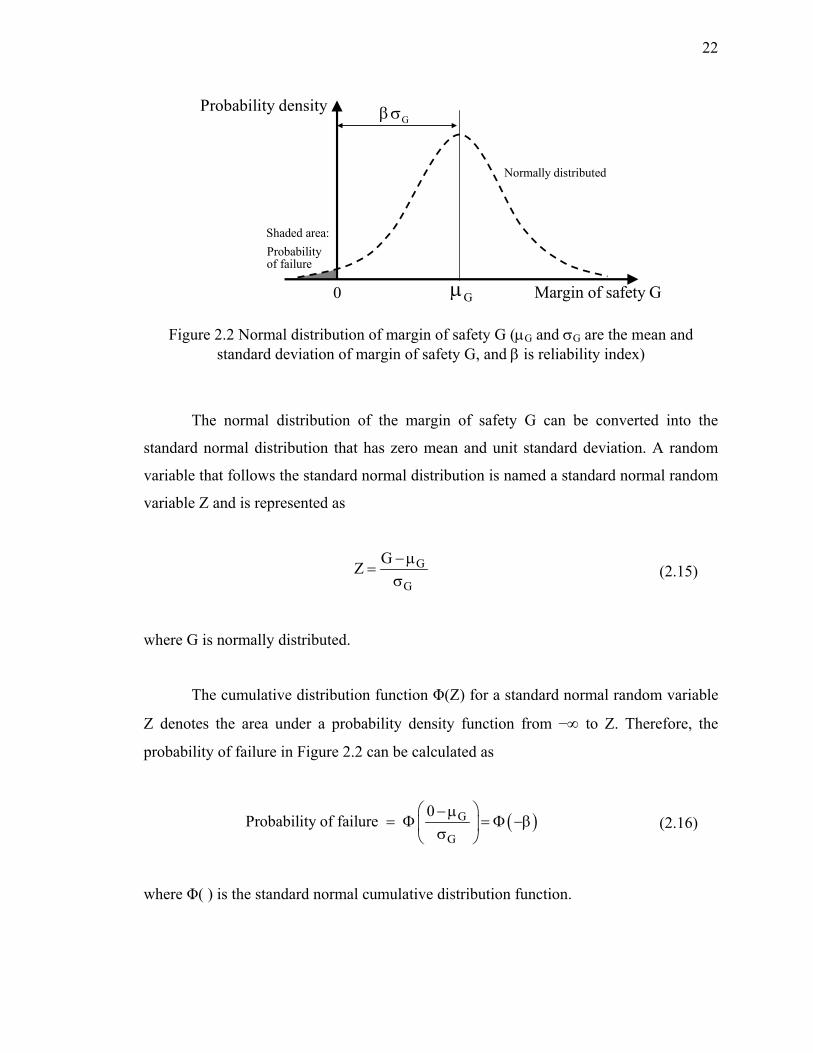
22
Probability density
Margin of safety G0 Gμ
Gβσ
Shaded area:Probabilityof failure
Normally distributed
Figure 2.2 Normal distribution of margin of safety G (μG and σG are the mean and standard deviation of margin of safety G, and β is reliability index)
The normal distribution of the margin of safety G can be converted into the
standard normal distribution that has zero mean and unit standard deviation. A random
variable that follows the standard normal distribution is named a standard normal random
variable Z and is represented as
G
G
GZ − μ=
σ (2.15)
where G is normally distributed.
The cumulative distribution function Φ(Z) for a standard normal random variable
Z denotes the area under a probability density function from −∞ to Z. Therefore, the
probability of failure in Figure 2.2 can be calculated as
( )G
G
0Probability of failure ⎛ ⎞− μ
= Φ = Φ −β⎜ ⎟σ⎝ ⎠ (2.16)
where Φ( ) is the standard normal cumulative distribution function.

23
Eq. (2.16) is the mathematical expression of the one-to-one relationship between
the target probability of failure and the target reliability index when Q and R are
uncorrelated and normally distributed. If the distribution of total load and resistance are
unpredictable or indefinable, it is impossible to correlate the target probability of failure
with a corresponding reliability index. In this case, we can only use a target probability of
failure criterion for LRFD.
A target probability of failure is used in LRFD of slopes because its analysis is
very complicated and the distributions of the total load (driving moment) and resistance
(resisting moment) are irregular or arbitrary. For the method of estimating a probability
of failure of slopes, Monte Carlo simulations are used. Monte Carlo simulation is the
repetitive process of generating very large numbers of values that can reproduce the
probability distributions of the parameters and models. The advantage of this method is
its simplicity, but the method requires a large number of simulations and thus is
computationally costly.
A target reliability index criterion is employed in LRFD of MSE walls because
the distributions of the total load and resistance, as well as the parameters that are used in
the analysis, are either normally distributed or can be approximated to be normally
distributed. The First-Order Reliability Method (FORM) is used for LRFD of MSE walls
to calculate a reliability index. FORM is the method that computes a reliability index β
using a geometric interpretation of the minimum distance between the point
corresponding to the mean values of the parameters used in the analysis (the peak point
of the probability distribution function of the parameters) and an ultimate limit state
surface. The basic concepts of probability theory, Monte Carlo simulation and FORM are
introduced in Appendix B.
2.4.1. Target probability of failure Pf
Chowdhury and Flentje (2002) suggested values of target probability of failure for a
natural slope for different slope types and locations (urban versus nonurban areas). A
lower value of target probability of failure is suggested for slopes whose failure will have
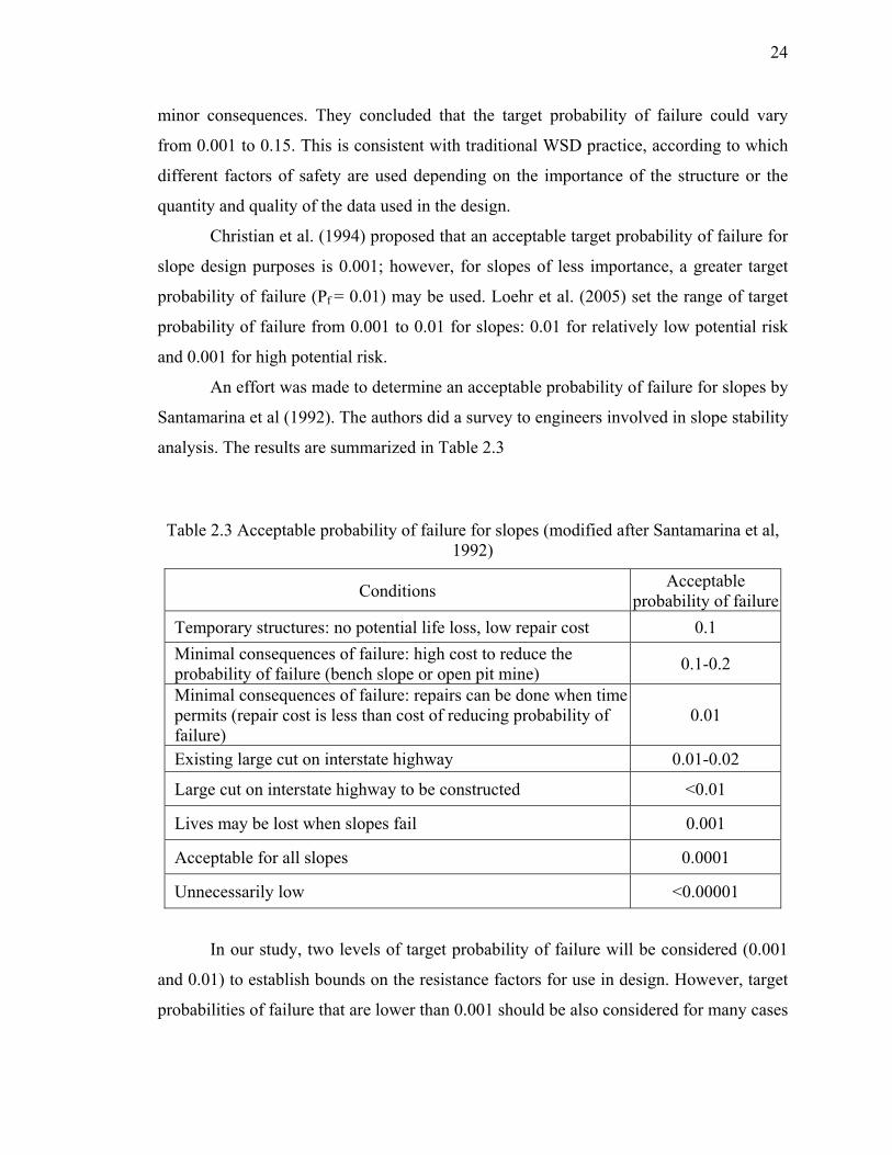
24
minor consequences. They concluded that the target probability of failure could vary
from 0.001 to 0.15. This is consistent with traditional WSD practice, according to which
different factors of safety are used depending on the importance of the structure or the
quantity and quality of the data used in the design.
Christian et al. (1994) proposed that an acceptable target probability of failure for
slope design purposes is 0.001; however, for slopes of less importance, a greater target
probability of failure (Pf = 0.01) may be used. Loehr et al. (2005) set the range of target
probability of failure from 0.001 to 0.01 for slopes: 0.01 for relatively low potential risk
and 0.001 for high potential risk.
An effort was made to determine an acceptable probability of failure for slopes by
Santamarina et al (1992). The authors did a survey to engineers involved in slope stability
analysis. The results are summarized in Table 2.3
Table 2.3 Acceptable probability of failure for slopes (modified after Santamarina et al, 1992)
Conditions Acceptable probability of failure
Temporary structures: no potential life loss, low repair cost 0.1 Minimal consequences of failure: high cost to reduce the probability of failure (bench slope or open pit mine) 0.1-0.2
Minimal consequences of failure: repairs can be done when time permits (repair cost is less than cost of reducing probability of failure)
0.01
Existing large cut on interstate highway 0.01-0.02
Large cut on interstate highway to be constructed <0.01
Lives may be lost when slopes fail 0.001
Acceptable for all slopes 0.0001
Unnecessarily low <0.00001
In our study, two levels of target probability of failure will be considered (0.001
and 0.01) to establish bounds on the resistance factors for use in design. However, target
probabilities of failure that are lower than 0.001 should be also considered for many cases
25
of interest in practice including important structures like dams or large levees, whose
failure may cause loss of many lives. Definitive values of LFs and RFs for slopes
therefore will require additional analysis.
2.4.2. Target reliability index βT
The target reliability index βT for LRFD of MSE walls may vary with the importance of
the wall. In this study, different values of target reliability indices (βT = 2.0, 2.5, 3.0, and
3.5) are used for LRFD of MSE walls. A target reliability index of 3.0 is widely used in
probabilistic stability analysis of geotechnical structures (Foye, 2004; Ellingwood et al.,
1980; and Palkowsky et al., 2004). Foye (2004) also stated that βT of 3.0 is widely used
in structural practice; therefore, the substructures that are supporting superstructures
should have a consistent βT. In general, AASHTO LRFD bridge design specification
(2007) uses a target reliability index of 3.5 for main elements and components whose
failure may cause bridge failure. For elements or components that are not failure-critical,
lower values of target reliability index (target reliability index less than 3.5) may be
considered. The lower values of βT (2.0 and 2.5) may be used by designers who want to
have less conservatism in MSE wall design.
When FORM is used in analysis, a target reliability index can be converted into a
target probability of failure using Eq. (2.16) because of their unique relationship under
the assumption that both total load and resistance follow a normal distribution. Table 2.4
shows the values of target probability of failure corresponding to various values of
reliability index. If the variable is not normally distributed but follows a certain type of
distribution, the changing of a nonnormally distributed variable into a normally
distributed variable is possible using the concept of an equivalent mean and standard
deviation.

26
Table 2.4 The equivalent values of target probability of failure for a corresponding target reliability index
Target reliability index βT Target probability of failure Pf 1 0.16
1.5 0.067 2 0.023
2.5 0.0062 3 0.0013
3.5 0.00023 4 0.000032
4.5 0.0000034 5 0.00000029
The conversion of a target probability of failure into an equivalent target
reliability index is conducted typically using the chart for standard normal curve area.
This chart is provided in most books on statistics. For example, βT = 3 corresponds to Z =
−3 in Eq. (2.16); therefore, the probability that corresponds to Z = −3 is found to be 0.013
from the chart.

28
PART II - LRFD OF SLOPES
The primary goal of a slope design is the economical selection of slope angle or height
while achieving a satisfying level of safety for the slope. To evaluate the stability of
slopes, it is important to understand the topography, geological condition, the seasonal
variation of groundwater, and the external load characteristics of the slopes. The
examination of whether the slope stability under short-term condition or that under long-
term condition is the worst case is also required. After examining these factors, a slope
stability analysis is conducted using the slope geometry, soil strength parameters, soil
unit weights, and external loads reflecting these factors.
Slope stability has been traditionally evaluated using WSD and a factor of safety.
For slope design purposes, design specifications provide a minimum factor of safety that
must be exceeded. However, the proposed minimum factor of safety is employed for all
types of slopes regardless of (1) the degrees of uncertainty associated with loads inducing
instability of the slope and the resistance against the loads and (2) the geometry of the
slope. LRFD of slopes accounts for these two conditions in slope design so that LRFD
more effectively pursues the primary goal for slope design, which is an economical and
safe design.
The slope part of this report (chapter 3 through chapter 5) introduces (1) an
algorithm for LRFD development for slopes, (2) an assessment of uncertainty associated
with soil parameter measurements, (3) a representation of spatial soil variability using
Gaussian random field theory, and (4) a calculation of optimum factors for LRFD of
slopes.
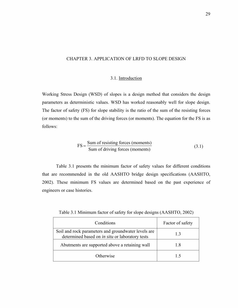
29
CHAPTER 3. APPLICATION OF LRFD TO SLOPE DESIGN
3.1. Introduction
Working Stress Design (WSD) of slopes is a design method that considers the design
parameters as deterministic values. WSD has worked reasonably well for slope design.
The factor of safety (FS) for slope stability is the ratio of the sum of the resisting forces
(or moments) to the sum of the driving forces (or moments). The equation for the FS is as
follows:
Sum of resisting forces (moments)FSSum of driving forces (moments)
= (3.1)
Table 3.1 presents the minimum factor of safety values for different conditions
that are recommended in the old AASHTO bridge design specifications (AASHTO,
2002). These minimum FS values are determined based on the past experience of
engineers or case histories.
Table 3.1 Minimum factor of safety for slope designs (AASHTO, 2002)
Conditions Factor of safety
Soil and rock parameters and groundwater levels are determined based on in situ or laboratory tests 1.3
Abutments are supported above a retaining wall 1.8
Otherwise 1.5

30
These minimum factors of safety values do not vary with the slope geometry or
the levels of uncertainties of loads and soil strength parameters. Therefore, the current
WSD proposes a single value of factor of safety that may be extremely conservative for
some slopes with small slope angle and a lesser amount of load and strength parameter
uncertainty. LRFD of slopes guarantees that a probability of failure of a slope does not
exceed the target probability of failure if the development of the LRFD method for slopes
is done in a rational way.
To develop LRFD for slopes, the assessment of the uncertainties of the
parameters must be done with great care. For example, the assessment of the
uncertainties of soil parameters is likely to be erroneous if limited data are obtained for
natural slopes or slopes with large dimensions. In addition, development of LRFD for
slopes is very expensive in terms of computation time and effort. However, once a well-
established LRFD method for slopes is developed, it will produce more consistent and
reliable results for slope design than WSD.
In this study, Gaussian random field theory is used to reproduce the uncertainty of
the strength parameters and the unit weight of the soil slopes. In addition, the ULS for
slope stability is defined using the Bishop simplified method with a factor of safety equal
to unity.
The current AASHTO LRFD design specifications (2007) use a resistance factor
that is equal to the inverse of the factor of safety because it assumes all the load factors
for different types of loads associated with slope designs to be equal to one (LFi = 1).
Although the use of LF equal to one for all types of loads is not reasonable, this study
will not address specifically what those values should be. This may be possible to do after
a substantial number of reliability analyses, covering various geometries of slopes and
site conditions (location of soil layers, values of soil parameters, and so on), is done.
However, the six examples given in chapter 5 provide elements upon which
recommendation of suitable LF values may be possible.

31
3.2. Bishop Simplified Method
Bishop (1955) proposed the Bishop Simplified Method (BSM), which is applicable to
circular slip surfaces. BSM is a method of slices that divides the sliding mass vertically
into many slices, as shown in Figure 3.1. There are other types of methods of slices, such
as Fellenius’ method, Janbu’s method, Spencer’s method and others. The methods differ
in the assumption about inter-slice forces and the shape of the slip surface. Despite the
difference in the assumption about inter-slice forces, the calculated FS using BSM is
comparable to those using more rigorous methods, such as Spencer’s method for a given
circular slip surface (the FS from BSM is slightly less than those from the other two). In
general, the selection of the method for slope stability analysis is less important than the
determination of the strength parameters and the geometry of the slopes. Additionally,
any resistance factors found to be appropriate for BSM would be slightly conservative for
a more rigorous method, such as Spencer’s method.
1l
2l3l
nl
4l
n 1−l
n 2−l
center of moment
circular slip surface
Figure 3.1 Method of slices (li is the length of the bottom of ith slice; i=1,···,n)
Figure 3.2 represents the forces acting on an arbitrary slice of the soil mass above
the potential slip surface. For the inter-slice forces of each slice (X and Y in Figure 3.2),
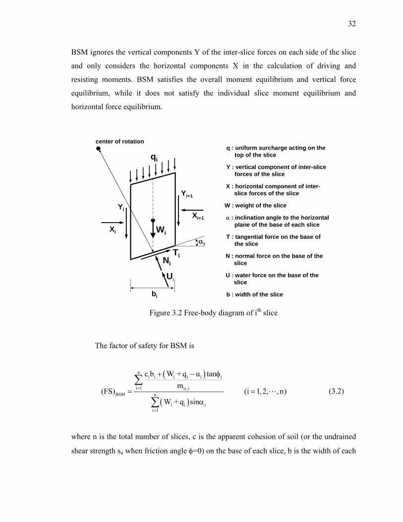
32
BSM ignores the vertical components Y of the inter-slice forces on each side of the slice
and only considers the horizontal components X in the calculation of driving and
resisting moments. BSM satisfies the overall moment equilibrium and vertical force
equilibrium, while it does not satisfy the individual slice moment equilibrium and
horizontal force equilibrium.
W : weight of the slice
qi
αi
Ni
bi
Ui
Ti
center of rotation
Yi
Yi+1
Xi
Xi+1
q : uniform surcharge acting on thetop of the slice
Y : vertical component of inter-sliceforces of the slice
X : horizontal component of inter-slice forces of the slice
Wi
α : inclination angle to the horizontalplane of the base of each slice
T : tangential force on the base ofthe slice
N : normal force on the base of the slice
U : water force on the base of theslice
b : width of the slice
Figure 3.2 Free-body diagram of ith slice
The factor of safety for BSM is
( )
( )
ni i i i i i
i 1 ,iBSM n
i i ii 1
c b W + q u tanm
(FS) (i 1,2, , n)W + q sin
= α
=
+ − φ
= =α
∑
∑L (3.2)
where n is the total number of slices, c is the apparent cohesion of soil (or the undrained
shear strength su when friction angle φ=0) on the base of each slice, b is the width of each

33
slice, W is the soil weight of each slice, q is the uniform surcharge acting on the top of
each slice, u is the water force acting on the base of each slice, φ is the friction angle on
the base of each slice, and α is the angle with the horizontal of the base of each slice. The
term mα,i is defined as follows:
i i,i i
tan tanm cos 1 (i 1,2, , n)FSα
α φ⎛ ⎞= α + =⎜ ⎟⎝ ⎠
L (3.3)
When all the parameters that are used in the analysis are deterministic, a single
value of FS is calculated for a trial slip surface. The generation of a large number of trial
slip surfaces is required to find the most critical slip surface for the given slope. The most
critical slip surface corresponds to the slip surface that has the lowest FS among the FS
values for all trial slip surfaces. However, for LRFD of slopes, the limit-state equation for
BSM is defined for FS = 1. Therefore, to represent this limit-state equation, Eq. (3.2) can
be revised as
( )( ) ( )
n ni i i i i i
i i ii 1 i 1i i i
c b W + q u tanW + q sin 0
cos 1 tan tan
(i 1,2, , n)
= =
+ − φ− α =
α + α φ
=
∑ ∑
L
(3.4)
3.3. Algorithm for LRFD of Slopes
In our analysis, we only consider the following parameters to have uncertainty: (1) soil
unit weight γ, (2) undrained shear strength su, (3) apparent cohesion c, and (4) friction
angle φ. The uncertainty in the slope geometry is neglected. We also do not consider pore
pressure or other water conditions because these are highly time-dependent. Instead,
designers should work with worst-case groundwater assumptions.

34
The optimum resistance factor and load factors are calculated using the algorithm
shown in Figure 3.3. There are two loops in this algorithm: (1) the iterative process to
find the most critical slip surface for a given geometry and a given set of parameters
(undrained shear strength su, apparent cohesion c, friction angle φ, and soil unit weight γ);
and (2) the iteration to find the mean values of the parameters (su, c, φ, and γ) for which
the calculated probability of failure is equal to the target probability of failure Pf.

35
Step 1. Select (Guess) expected values (means) and coefficient of variations (COVs) of ci (sui), φi, γi, and q (external loads) for each layer. (i=layer number)
Step 2. Generate Gaussian random fields for each parameter (ci (sui), φi, and γi) and superpose these fields.
Step 3. Generate a large number of trial slip surfaces and find the most critical slip surface. For the most critical slip surface, save the corresponding driving moments Md (both Md due to the self-weight of the soil and Md due to the external loads separately) and the resisting moment Mr.
Step 5. For the N most critical slip surfaces (corresponding to the N iterations), count the cases (n) for which total Md (a sum of Md due to self-weight of the soil and Md due to the external loads) is equal to or greater than Mr. Probability of failure = n/N.
Step 6. Single out the limit state that corresponds to Md/Mr = 1. Save the limit-state values of Md (both Md due to the self-weight of the soil and Md due to the external loads) and Mr.
Step 7. Calculate nominal values of ci (sui), φi, γi, and q by multiplying the bias factors of the parameters by their mean values for which the calculated probability of failure is equal to the target probability of failure.
Step 9. Calculate optimum values of RF, LFs, and RF which will be denoted by RF*, LF*s, and RF, respectively.
Step 4. Repeat “Step 2” and “Step 3” N times.
Probability of failure calculated in “Step 5”= target probability of failure Pf
No
Yes
Step 8. Run deterministic limit equilibrium analysis using these nominal values, find the most critical slip surface, and calculate the nominal Md (Md due to the self-weight and Md due to the external loads) and the nominal Mr for the most critical slip surface..
Figure 3.3 Algorithm for LRFD of slopes

36
A large computational effort is required to find the combination of expected
values and the corresponding COVs of ci (sui), φi, γi, and q that correspond to the target
probability of failure. The algorithm is coded using FORTRAN. Finding one set of
appropriate ci (sui), φi, γi, and q values that satisfy the target probability of failure for a
three-layer soil slope has taken at least a week even though we have used a high-
performance computer (Intel Core 2 CPU [email protected] with 2GB of RAM) for the
analysis.
In Step 1, we select the initial expected values and the corresponding COVs of ci
(sui), φi, γi, and q (Figure 3.4). Ideally, we would guess perfectly, and these values would
produce the target probability of failure Pf. In reality, we will need to adjust these values
based on how far the calculated probability of failure is from the target probability of
failure. A good guess of the values of these parameters will naturally save time and effort.
Layer 1
Layer 2
Layer 3
c1 (su1), φ1, γ1
c2 (su2), φ2, γ2
c3 (su3), φ3, γ3
q
Figure 3.4 Geometry and soil parameters of the slope
Next, in Step 2, we generate a Gaussian random field for each parameter for each
layer. For example, if the slope consists of three layers each with its own c (su), φ, and γ,
the total number of Gaussian random fields that are required in this step will be nine. A
Gaussian random field of each parameter will be shown as an array of values that have
constant spacing as shown in Figure 3.5. The values at every point are different from

37
point to point as dictated by the Gaussian random field; however, the expected value and
the standard deviation of the parameter (ci, (sui), φi, and γi) are the same at each point. The
generation of Gaussian random fields will be discussed in detail in the next chapter.
Layer 1
Layer 2
Layer 3
Figure 3.5 The array of data points generated by Gaussian random field theory
Nonspatial variability, such as a measurement error, can be represented by a
purely random field such that each value within the random field is independent of all
other values, has zero mean and has the variance of the nonspatial variability. This can
then be added to the Gaussian random field generated earlier.
Step 3 consists of finding the most critical slip surface and the corresponding
values of the driving moments and the resisting moment from a large number of trial slip
surfaces (Figure 3.6). The factor of safety (FS) is the lowest for the most critical slip
surface. The procedure of finding the most critical slip surface is the same as that of
conventional slope stability analysis.
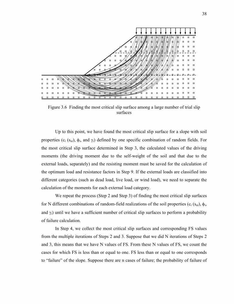
38
Figure 3.6 Finding the most critical slip surface among a large number of trial slip surfaces
Up to this point, we have found the most critical slip surface for a slope with soil
properties (ci (sui), φi, and γi) defined by one specific combination of random fields. For
the most critical slip surface determined in Step 3, the calculated values of the driving
moments (the driving moment due to the self-weight of the soil and that due to the
external loads, separately) and the resisting moment must be saved for the calculation of
the optimum load and resistance factors in Step 9. If the external loads are classified into
different categories (such as dead load, live load, or wind load), we need to separate the
calculation of the moments for each external load category.
We repeat the process (Step 2 and Step 3) of finding the most critical slip surfaces
for N different combinations of random-field realizations of the soil properties (ci (sui), φi,
and γi) until we have a sufficient number of critical slip surfaces to perform a probability
of failure calculation.
In Step 4, we collect the most critical slip surfaces and corresponding FS values
from the multiple iterations of Steps 2 and 3. Suppose that we did N iterations of Steps 2
and 3, this means that we have N values of FS. From these N values of FS, we count the
cases for which FS is less than or equal to one. FS less than or equal to one corresponds
to “failure” of the slope. Suppose there are n cases of failure; the probability of failure of

39
the slope will then be n divided by N. If the probability of failure calculated in Step 5 is
not equal to or is not very close to the target probability of failure Pf (in our analysis, Pf =
0.001 or 0.01), we go back to Step 1 and change the initial expected values (mean values)
of the soil parameters, repeat the steps and keep adjusting these mean values until the
target probability of failure is met.
Once the target probability of failure is met, we single out the case where FS is
equal to or is very close to one out of N cases. This case, with FS = 1, corresponds to the
ULS for the target probability of failure. For the calculation of the optimum factors, we
must save the limit-state values of driving moments (the driving moment due to the self-
weight of the soil and that due to the external loads) and the resisting moment.
A conventional deterministic slope stability analysis is performed using the
nominal values of the soil parameters and external loads. Nominal values of the soil
properties are obtained by multiplying the bias factors of the parameters by their mean
values (for which the calculated probability of failure is equal to the target probability of
failure). From this deterministic analysis, we find the most critical slip surface and the
corresponding nominal values of the driving moments and the resisting moment.
In the final step (Step 9), the optimum resistance factor and load factors are
determined using the pre-calculated limit-state moments and nominal moments in Steps 5
and 6. Eq. (2.5) and Eq. (2.6) are used to calculate the optimum factors. In Eq. (2.5) and
Eq. (2.6), the driving moments Md and the resisting moment Mr will replace loads Q and
resistance R, respectively.
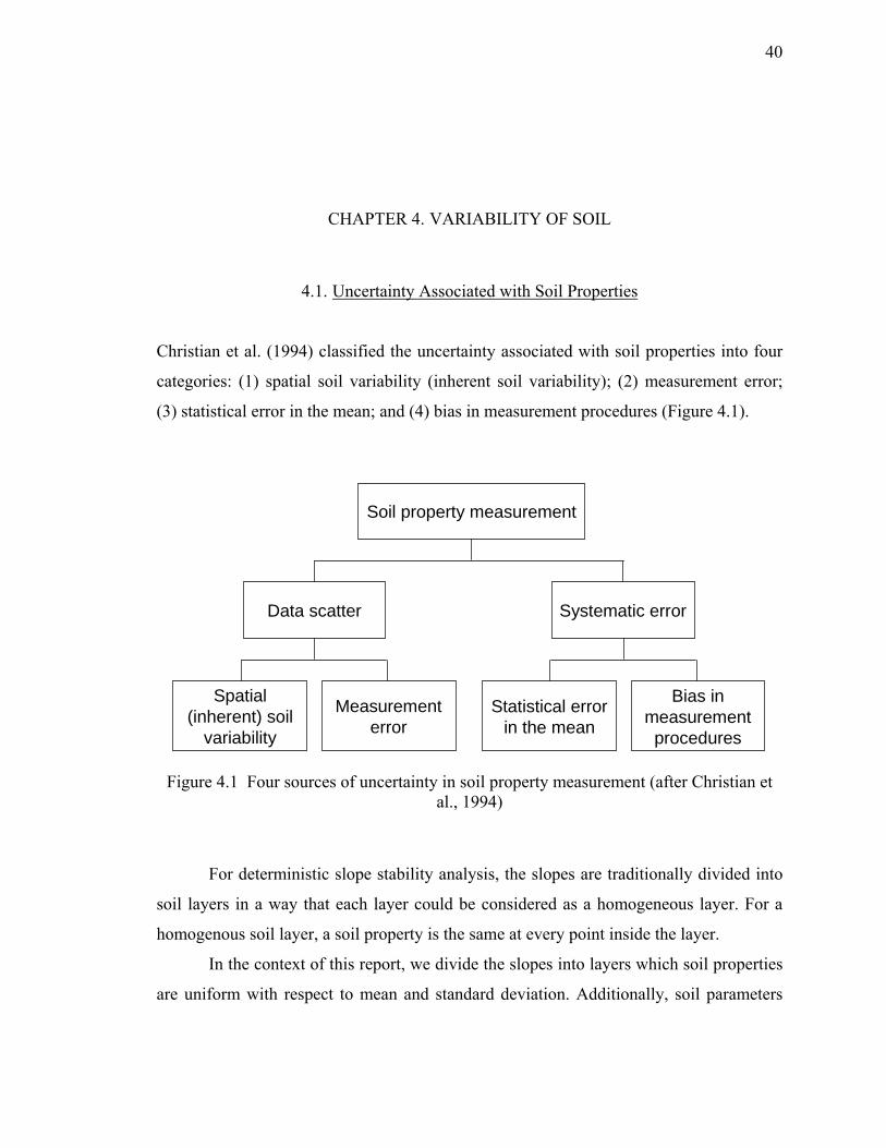
40
CHAPTER 4. VARIABILITY OF SOIL
4.1. Uncertainty Associated with Soil Properties
Christian et al. (1994) classified the uncertainty associated with soil properties into four
categories: (1) spatial soil variability (inherent soil variability); (2) measurement error;
(3) statistical error in the mean; and (4) bias in measurement procedures (Figure 4.1).
Soil property measurement
Systematic errorData scatter
Spatial (inherent) soil
variability
Measurement error
Statistical error in the mean
Bias in measurement
procedures
Figure 4.1 Four sources of uncertainty in soil property measurement (after Christian et al., 1994)
For deterministic slope stability analysis, the slopes are traditionally divided into
soil layers in a way that each layer could be considered as a homogeneous layer. For a
homogenous soil layer, a soil property is the same at every point inside the layer.
In the context of this report, we divide the slopes into layers which soil properties
are uniform with respect to mean and standard deviation. Additionally, soil parameters

41
are governed by isotropic correlation coefficient functions. These soil layers may be
referred to as “statistically homogeneous.”
If the uncertainty associated with soil property measurement does not exist, the
mean and standard deviation of a soil parameter of a statistically homogeneous soil layer
are the mean and the standard deviation of the real in situ soil property. The variability of
the real in situ soil property corresponds to that of spatial soil variability. However, the
direct assessment of spatial soil variability is impossible because the exact real in situ soil
property is unattainable in reality. Therefore, to simulate spatial soil variability, we must
separate spatial soil variability from uncertainties associated with soil property
measurement.
In reality, the four sources of uncertainty in soil property measurement (Figure
4.1) are grouped together so that it is hard to differentiate between them. However, an
effort has been made to separate these four sources step by step. Figure 4.2 illustrates the
spatial variability of a soil property. For the purpose of slope stability analysis, we
assume that there is no directional trend of the mean of soil parameters within a
statistically homogeneous layer, as shown in Figure 4.2.
Due to spatial soil variability, the soil properties in a statistically homogeneous
layer change with the location. The scatter of real in situ values around their mean, as
shown in Figure 4.2, is due to spatial soil variability.
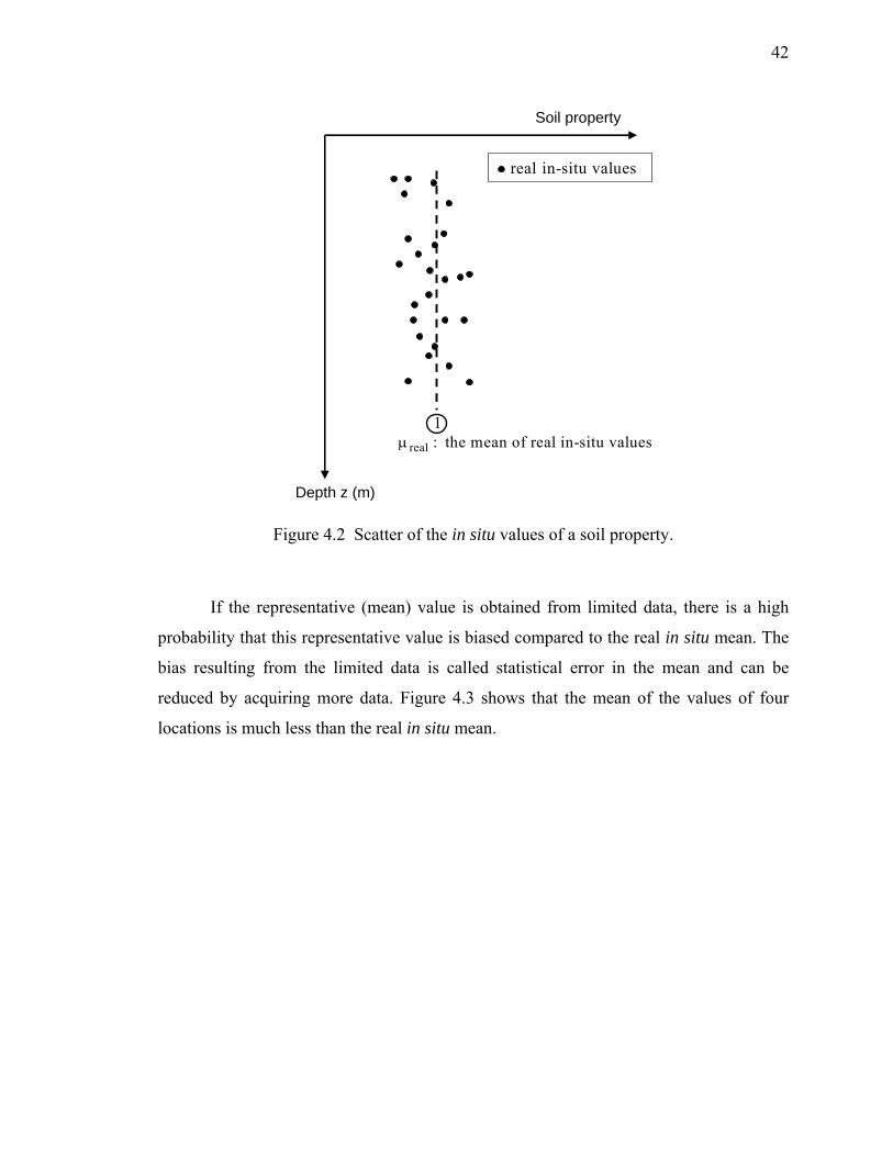
42
Soil property
Depth z (m)
1real : the mean of real in-situ valuesμ
real in-situ values
Figure 4.2 Scatter of the in situ values of a soil property.
If the representative (mean) value is obtained from limited data, there is a high
probability that this representative value is biased compared to the real in situ mean. The
bias resulting from the limited data is called statistical error in the mean and can be
reduced by acquiring more data. Figure 4.3 shows that the mean of the values of four
locations is much less than the real in situ mean.
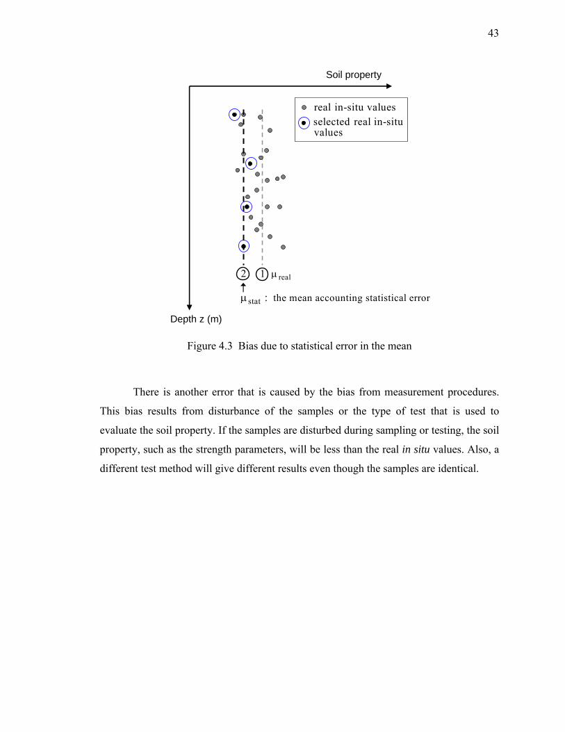
43
stat the mean accounting statistical error: μ
selected real in-situ values
Soil property
1 realμ2
Depth z (m)
real in-situ values
Figure 4.3 Bias due to statistical error in the mean
There is another error that is caused by the bias from measurement procedures.
This bias results from disturbance of the samples or the type of test that is used to
evaluate the soil property. If the samples are disturbed during sampling or testing, the soil
property, such as the strength parameters, will be less than the real in situ values. Also, a
different test method will give different results even though the samples are identical.
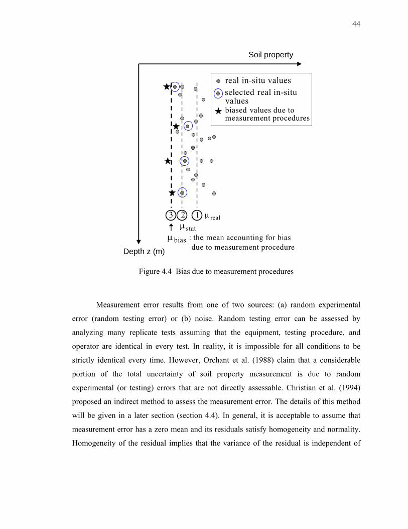
44
biased values due to measurement procedures
Soil property
Depth z (m)
statμ1 realμ23
bias : the mean accounting for bias due to measurement procedure
μ
real in-situ valuesselected real in-situ values
Figure 4.4 Bias due to measurement procedures
Measurement error results from one of two sources: (a) random experimental
error (random testing error) or (b) noise. Random testing error can be assessed by
analyzing many replicate tests assuming that the equipment, testing procedure, and
operator are identical in every test. In reality, it is impossible for all conditions to be
strictly identical every time. However, Orchant et al. (1988) claim that a considerable
portion of the total uncertainty of soil property measurement is due to random
experimental (or testing) errors that are not directly assessable. Christian et al. (1994)
proposed an indirect method to assess the measurement error. The details of this method
will be given in a later section (section 4.4). In general, it is acceptable to assume that
measurement error has a zero mean and its residuals satisfy homogeneity and normality.
Homogeneity of the residual implies that the variance of the residual is independent of
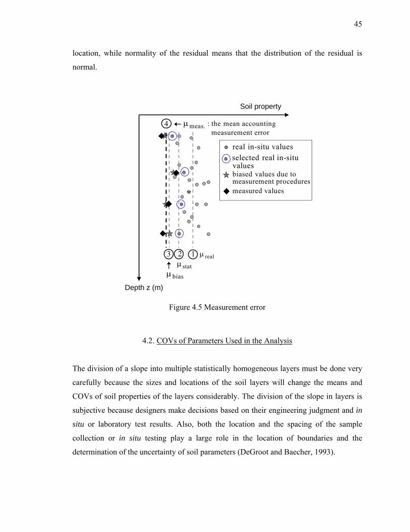
45
location, while normality of the residual means that the distribution of the residual is
normal.
Soil property
Depth z (m)
statμ1 realμ23
biasμ
4 meas. : the mean accounting measurement error
μ
biased values due to measurement procedures
real in-situ valuesselected real in-situ values
measured values
Figure 4.5 Measurement error
4.2. COVs of Parameters Used in the Analysis
The division of a slope into multiple statistically homogeneous layers must be done very
carefully because the sizes and locations of the soil layers will change the means and
COVs of soil properties of the layers considerably. The division of the slope in layers is
subjective because designers make decisions based on their engineering judgment and in
situ or laboratory test results. Also, both the location and the spacing of the sample
collection or in situ testing play a large role in the location of boundaries and the
determination of the uncertainty of soil parameters (DeGroot and Baecher, 1993).
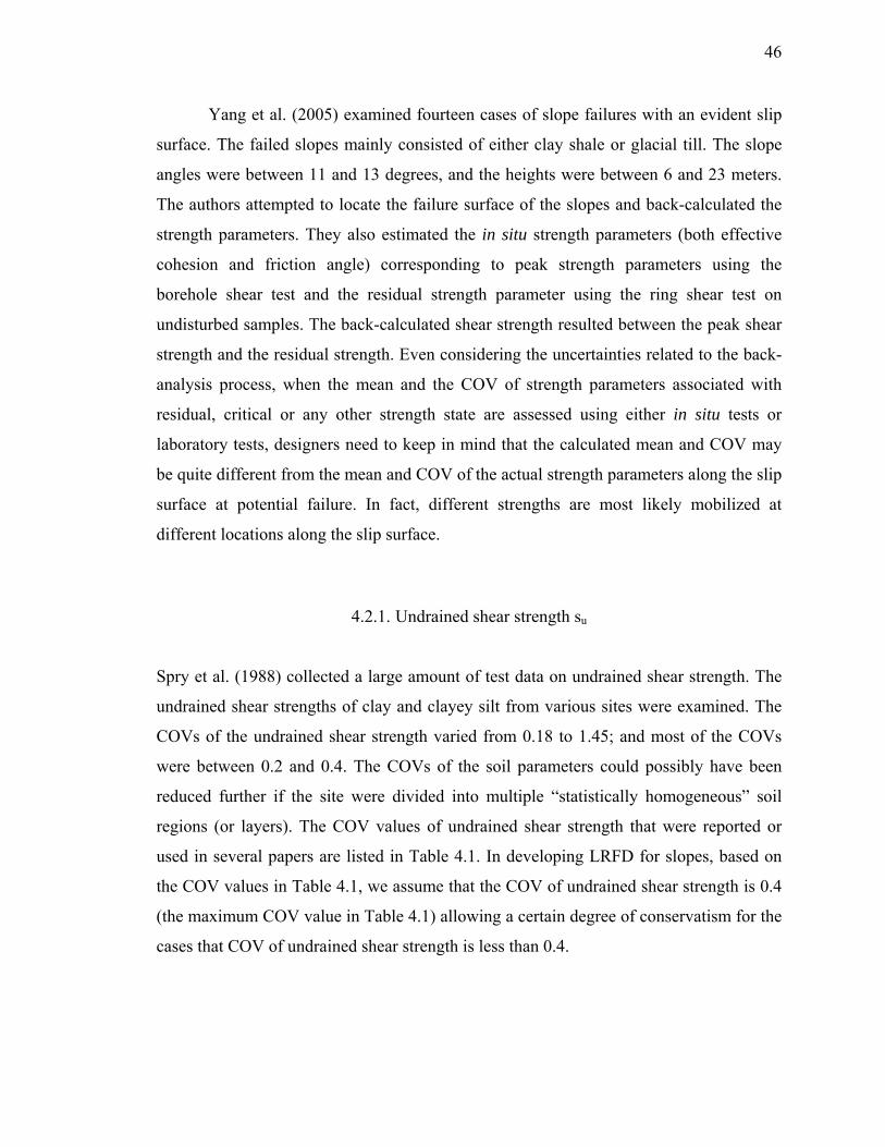
46
Yang et al. (2005) examined fourteen cases of slope failures with an evident slip
surface. The failed slopes mainly consisted of either clay shale or glacial till. The slope
angles were between 11 and 13 degrees, and the heights were between 6 and 23 meters.
The authors attempted to locate the failure surface of the slopes and back-calculated the
strength parameters. They also estimated the in situ strength parameters (both effective
cohesion and friction angle) corresponding to peak strength parameters using the
borehole shear test and the residual strength parameter using the ring shear test on
undisturbed samples. The back-calculated shear strength resulted between the peak shear
strength and the residual strength. Even considering the uncertainties related to the back-
analysis process, when the mean and the COV of strength parameters associated with
residual, critical or any other strength state are assessed using either in situ tests or
laboratory tests, designers need to keep in mind that the calculated mean and COV may
be quite different from the mean and COV of the actual strength parameters along the slip
surface at potential failure. In fact, different strengths are most likely mobilized at
different locations along the slip surface.
4.2.1. Undrained shear strength su
Spry et al. (1988) collected a large amount of test data on undrained shear strength. The
undrained shear strengths of clay and clayey silt from various sites were examined. The
COVs of the undrained shear strength varied from 0.18 to 1.45; and most of the COVs
were between 0.2 and 0.4. The COVs of the soil parameters could possibly have been
reduced further if the site were divided into multiple “statistically homogeneous” soil
regions (or layers). The COV values of undrained shear strength that were reported or
used in several papers are listed in Table 4.1. In developing LRFD for slopes, based on
the COV values in Table 4.1, we assume that the COV of undrained shear strength is 0.4
(the maximum COV value in Table 4.1) allowing a certain degree of conservatism for the
cases that COV of undrained shear strength is less than 0.4.
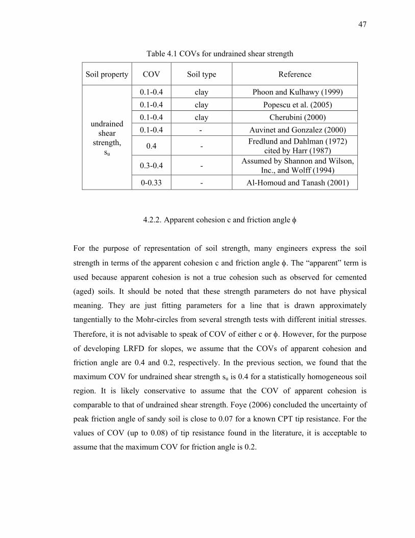
47
Table 4.1 COVs for undrained shear strength
Soil property COV Soil type Reference
undrained shear
strength, su
0.1-0.4 clay Phoon and Kulhawy (1999) 0.1-0.4 clay Popescu et al. (2005) 0.1-0.4 clay Cherubini (2000) 0.1-0.4 - Auvinet and Gonzalez (2000)
0.4 - Fredlund and Dahlman (1972) cited by Harr (1987)
0.3-0.4 - Assumed by Shannon and Wilson, Inc., and Wolff (1994)
0-0.33 - Al-Homoud and Tanash (2001)
4.2.2. Apparent cohesion c and friction angle φ
For the purpose of representation of soil strength, many engineers express the soil
strength in terms of the apparent cohesion c and friction angle φ. The “apparent” term is
used because apparent cohesion is not a true cohesion such as observed for cemented
(aged) soils. It should be noted that these strength parameters do not have physical
meaning. They are just fitting parameters for a line that is drawn approximately
tangentially to the Mohr-circles from several strength tests with different initial stresses.
Therefore, it is not advisable to speak of COV of either c or φ. However, for the purpose
of developing LRFD for slopes, we assume that the COVs of apparent cohesion and
friction angle are 0.4 and 0.2, respectively. In the previous section, we found that the
maximum COV for undrained shear strength su is 0.4 for a statistically homogeneous soil
region. It is likely conservative to assume that the COV of apparent cohesion is
comparable to that of undrained shear strength. Foye (2006) concluded the uncertainty of
peak friction angle of sandy soil is close to 0.07 for a known CPT tip resistance. For the
values of COV (up to 0.08) of tip resistance found in the literature, it is acceptable to
assume that the maximum COV for friction angle is 0.2.
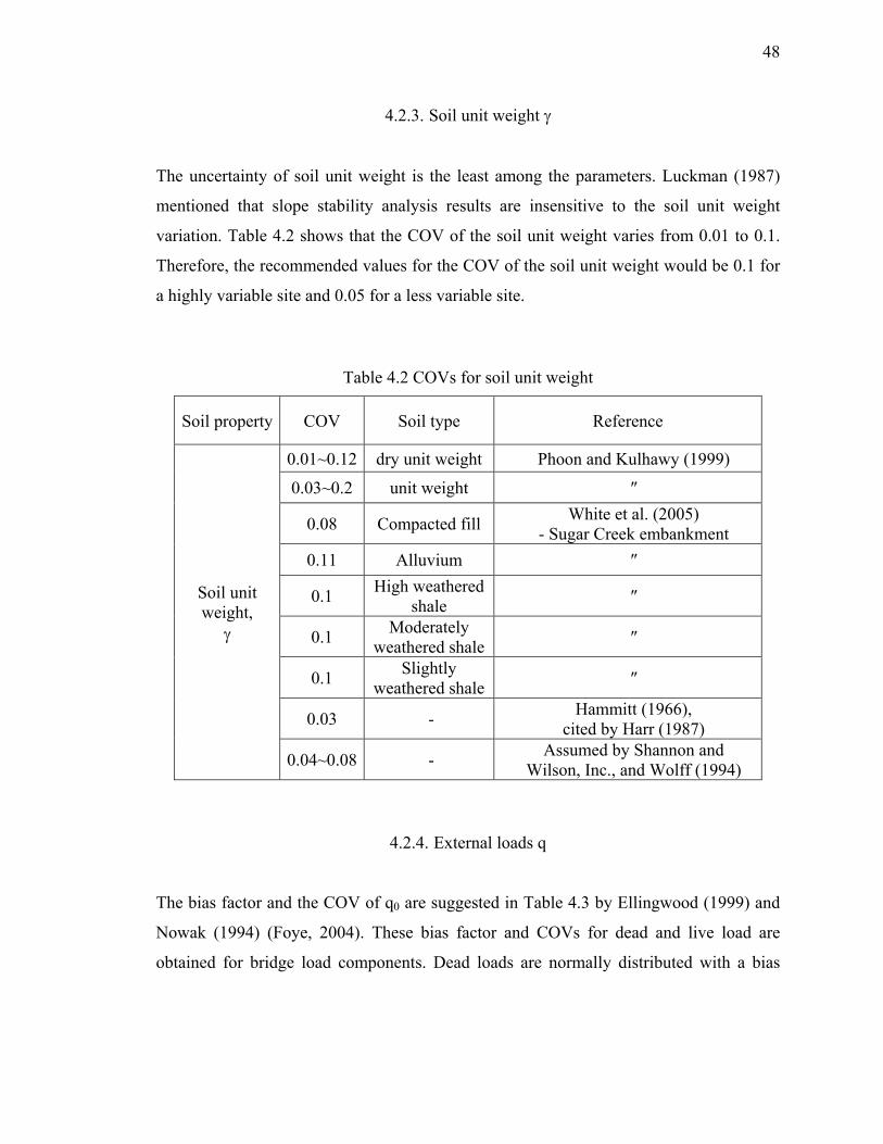
48
4.2.3. Soil unit weight γ
The uncertainty of soil unit weight is the least among the parameters. Luckman (1987)
mentioned that slope stability analysis results are insensitive to the soil unit weight
variation. Table 4.2 shows that the COV of the soil unit weight varies from 0.01 to 0.1.
Therefore, the recommended values for the COV of the soil unit weight would be 0.1 for
a highly variable site and 0.05 for a less variable site.
Table 4.2 COVs for soil unit weight
Soil property COV Soil type Reference
Soil unit weight,
γ
0.01~0.12 dry unit weight Phoon and Kulhawy (1999)
0.03~0.2 unit weight ″
0.08 Compacted fill White et al. (2005) - Sugar Creek embankment
0.11 Alluvium ″
0.1 High weathered shale ″
0.1 Moderately weathered shale ″
0.1 Slightly weathered shale ″
0.03 - Hammitt (1966), cited by Harr (1987)
0.04~0.08 - Assumed by Shannon and Wilson, Inc., and Wolff (1994)
4.2.4. External loads q
The bias factor and the COV of q0 are suggested in Table 4.3 by Ellingwood (1999) and
Nowak (1994) (Foye, 2004). These bias factor and COVs for dead and live load are
obtained for bridge load components. Dead loads are normally distributed with a bias

49
factor of 1.05 and a COV of 0.15, while the live load exhibits lognormal distribution with
a bias factor of 1.15 and a COV of 0.25.
Table 4.3 COVs and bias factors for dead load and live load
Variable Bias factor COV Distribution type
Dead load 1.05 0.15 Normal
Live load 1.15 0.25 Lognormal
(After Ellingwood, 1999 and Nowak,1994)
When we define the ULS of slope stability analysis for LRFD purposes, we
neglect the live loads that help stabilize a slope while we do consider the live loads that
are destabilizing the slope (Figure 4.6).
Stabilizing
Consider live surcharge
Destabilizing
Neglect live surcharge
Figure 4.6 Live loads considered in slope design (consider destabilizing live surcharges and neglect stabilizing live surcharges)

50
4.3. Spatial Variability of Soil Properties
The spatial variability of a soil property indicates the variation (or distribution) of the
scatter of the soil property values within a certain region. The spatial variability of a soil
property results mainly from soil deposition or weathering processes. Typically, the
degree of spatial soil variability in the vertical direction is higher than in the horizontal
direction because a deposition process occurs layer by layer.
Obtaining the true, exact value of a soil property at a point in a soil layer is
impossible. Strictly speaking, the soil properties of a statistically homogeneous soil layer,
which is divided based on engineering judgment and field test results, exhibit
heterogeneity at small scales. The soil properties within a statistically homogeneous soil
layer are considered as random variables following the theory for weakly stationary
Gaussian random field. A weakly stationary Gaussian random field model is used for the
representation of spatial soil variability. A random field is called “weakly stationary” if
the following conditions are met: (1) the expected value (mean) and variance are the
same at every point within the region of definition of the random field and (2) the
correlation coefficient function governs the random field by setting the degree of
correlation between the residuals of any two points. The correlation coefficient function
is a function of the separation distance between any two points within the random field.
The “Gaussian” term means that the random variable for which the field is defined
follows a Gaussian (normal) distribution function. From here forward, we will refer to
weakly stationary Gaussian random fields as simply Gaussian random fields.
4.3.1. Gaussian random field for spatial variability of soil properties
For our slope stability analysis, Gaussian random fields are generated using the Fourier
transform technique that Fenton (1990) proposed. Only an isotropic Gaussian random
field is considered. For an isotropic Gaussian random field, the correlation coefficient
function is a function of the distance of two points but it is independent of their direction.

51
4.3.1.1. Correlation coefficient function
Covariance (Cov) is the measure of how strong the correlation between two random
variables is. When two random variables are positively correlated (if one variable
increases, then the other variable also increases and vice versa), the Cov of these two
variables is a positive value. On the other hand, if two random variables are negatively
correlated (if one variable increases, the other variable decreases and vice versa), the
covariance has a negative sign. If two random variables are independent of each other,
then the covariance is equal to zero. The Covariance of two random variables (z1 and z2)
is
( ) ( )( )1 2 1 z1 2 z2Cov z , z E z z= − μ − μ⎡ ⎤⎣ ⎦ (4.1)
where μz1 and μz2 are the mean of z1 and z2, respectively.
The correlation coefficient of z1 and z2 is defined as the covariance of z1 and z2
divided by the product of their standard deviations (σz1 and σz2). The correlation
coefficient changes from -1 to 1 depending on the degree of correlation between the two
variables. The correlation coefficient ρ(z1, z2) of z1 and z2 is
( ) ( ) ( )( )1 z1 2 z21 21 2
z1 z2 z1 z2
E z zCov z , zz , z
− μ − μ⎡ ⎤⎣ ⎦ρ = =σ σ σ σ
(4.2)
where σz1 and σz2 are the standard deviations of z1 and z2, respectively.
The correlation coefficient could be defined for a single random variable z
depending on two different independent variables x and y. Suppose that we are
calculating the correlation coefficient of z between two points that are Δx apart in the
horizontal direction and Δy apart in the vertical direction. The covariance and correlation
coefficient in this case are

52
( ) ( ) ( ) ( ){ }z zCov z x, y , z x x, y y E z x, y z x x, y y+ Δ + Δ = − μ + Δ + Δ − μ⎡ ⎤ ⎡ ⎤ ⎡ ⎤⎣ ⎦ ⎣ ⎦ ⎣ ⎦ (4.3)
( ) ( )( ) ( ){ }z z
2z
E z x, y z x x, y yz x, y , z x x, y y
− μ + Δ + Δ − μ⎡ ⎤ ⎡ ⎤⎣ ⎦ ⎣ ⎦ρ + Δ + Δ =⎡ ⎤⎣ ⎦ σ (4.4)
where x and y are the random variables that define the location of the value z, and μz is
the mean of the random variable z in the space containing x, y, x + Δx, and y + Δy.
In the field, the values of a soil property at two close points are more likely to be
similar than those of two points that are far away from each other. An appropriate
correlation coefficient function should be selected so that it produces a reasonable
representation of the spatial soil variability observed in the domain within which the field
is defined. There are different types of correlation coefficient functions. Rackwitz (2000)
introduced six popular functions. However, Suzuki and Takara (1998) claim that the
correlation distance (which is directly related to scale of fluctuation), rather than the type
of correlation coefficient function, controls the representation of spatial variability.
Therefore, the selection of a correlation coefficient function does not have much
influence on the representation of spatial soil variability. An exponential correlation
coefficient function is commonly used in Gaussian random field generation. The
expression for this function for an isotropic random field is
( )f
2ss exps
⎛ ⎞ρ = −⎜ ⎟
⎝ ⎠ (4.5)
where s is separation distance and sf is an isotropic scale of fluctuation.
53
The value “2” inside the exponential correlation coefficient function Eq. (4.5) is
placed according to the definition of sf (the isotropic scale of fluctuation is equal to the
integral from negative infinity to infinity of the correlation coefficient function).
( )fs s ds∞
−∞= ρ∫ (4.6)
This scale of fluctuation sf is the parameter in the correlation coefficient function
that controls the degree of reduction in the correlation coefficient between any two points
that are s apart when s increases. Figure 4.7 shows how the exponential correlation
coefficient function varies with separation distance for different isotropic scales of
fluctuation (sf=1, 5, 10, and 20m).
0
0.2
0.4
0.6
0.8
1
1.2
0 5 10 15 20 25 30 35 40 45 50
Separation distance (m)
Cor
rela
tion
coef
ficie
nt
0
0.2
0.4
0.6
0.8
1
1.2
0 5 10 15 20 25 30 35 40 45 50
Separation distance (m)
Cor
rela
tion
coef
ficie
nt
fs =3m
fs =5m
fs =1m
fs =10m
Figure 4.7 Exponential correlation coefficient functions for different isotropic scales of fluctuation (in one-direction) (sf is the scale of fluctuation)
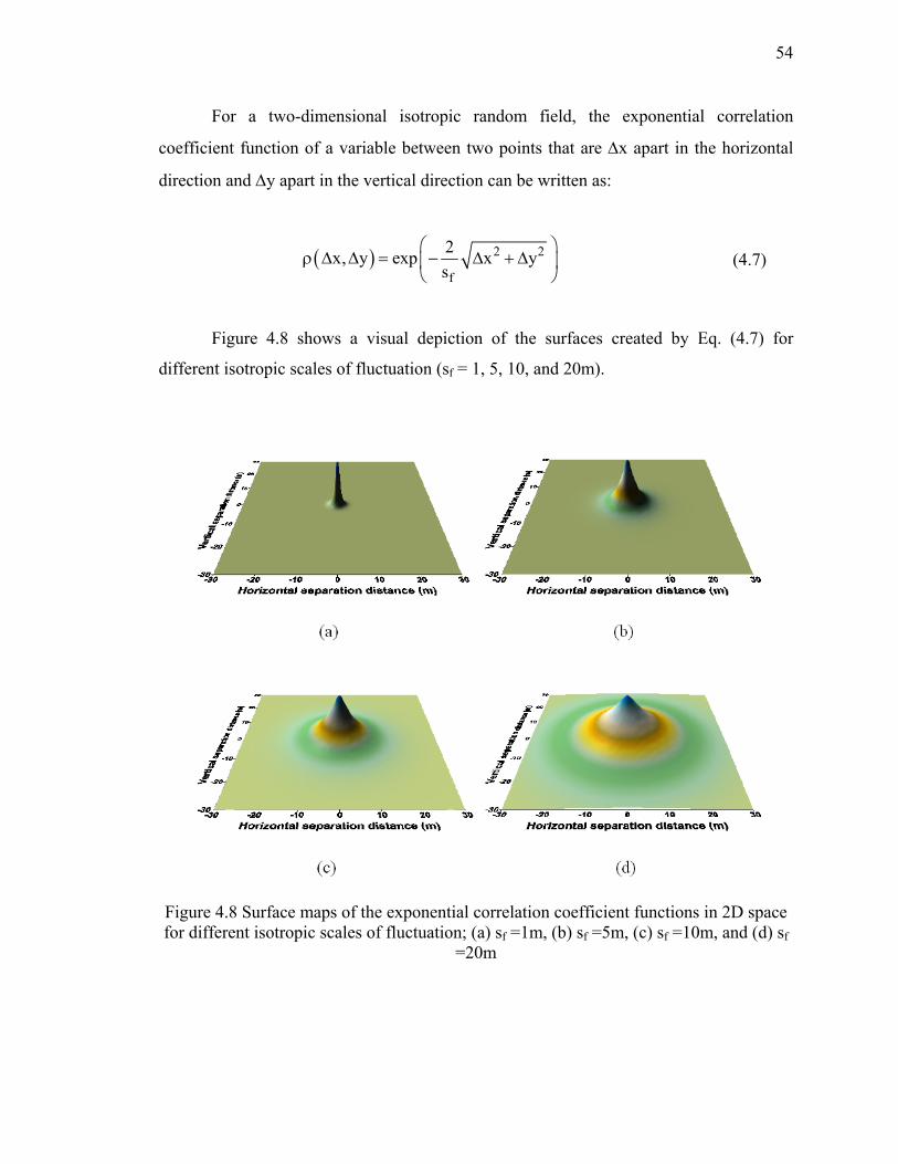
54
For a two-dimensional isotropic random field, the exponential correlation
coefficient function of a variable between two points that are Δx apart in the horizontal
direction and Δy apart in the vertical direction can be written as:
( ) 2 2
f
2x, y exp x ys
⎛ ⎞ρ Δ Δ = − Δ + Δ⎜ ⎟
⎝ ⎠ (4.7)
Figure 4.8 shows a visual depiction of the surfaces created by Eq. (4.7) for
different isotropic scales of fluctuation (sf = 1, 5, 10, and 20m).
Figure 4.8 Surface maps of the exponential correlation coefficient functions in 2D space for different isotropic scales of fluctuation; (a) sf =1m, (b) sf =5m, (c) sf =10m, and (d) sf
=20m

55
Fenton (1990) derived the exponential correlation coefficient function in 2D space
for an anisotropic random field:
( )22
f ,x f ,y
x yx, y exp 2s s
⎛ ⎞⎛ ⎞⎛ ⎞Δ Δ⎜ ⎟ρ Δ Δ = − + ⎜ ⎟⎜ ⎟⎜ ⎟⎜ ⎟ ⎜ ⎟⎜ ⎟⎝ ⎠ ⎝ ⎠⎝ ⎠
(4.8)
where sf,x and sf,y are the scales of fluctuation for the two reference directions x and y,
respectively.
4.3.1.2. Scale of fluctuation sf
Determination of a reliable scale of fluctuation sf is not easy because large
amounts of test data are required at narrow spacings. The smaller the value of sf is, the
less correlation exists between two nearby values of a variable. If the sf is an infinite
value, all the values of a random variable in a Gaussian random field are perfectly
correlated; therefore, the values are the same over the whole Gaussian random field, and
the layer is uniform. On the other hand, when sf is equal to zero, the values of the random
variable at all locations are independent of each other.

56
Table 4.4 shows the values of sf for the undrained shear strength that are reported or used
in analyses in the literature. The scale of fluctuation in the horizontal direction is much
larger than the one in the vertical direction.

57
Table 4.4 Horizontal and vertical scales of fluctuation of undrained shear strength
Soil property
Scale of fluctuation Soil type Reference Note
su
V
0.8~6.1 clay Phoon and Kulhawy (1999) 5~12 - Asaoka et al. (1982) 8.6 Chicago clay Wu (1974)
2.0~6.2 clay Phoon and Kulhawy (1999) VST 2~6 clay Asaoka and A-Grivas (1982) VST
2 sensitive clay Baecher (1982) VST 4 sensitive clay Chaisson et al. (1995) VST 4 - Soulie et al. (1990) VST
5 New Liskeard Varved clay
Vanmarcke (1977) and Lacasse and Ladd (1973) VST
2.4 soft clay, New York Asaoka and A-Grivas (1982) VST
6.2 soft clay, New York Asaoka and A-Grivas (1982) VST
H
46 sensitive clay DeGroot and Baecher (1993) VST 40 - Soulie et al. (1990) VST
46 New Liskeard varved clay
Vanmarcke (1977) and Lacasse and Ladd (1973) VST
2~10 - Al-Homoud and Tanash (2001)
I Less than 0.5, rarely more
than 10 - Rackwitz (2000)
(V: vertical, H: horizontal, I: isotropic, and VST: vane shear test)
The scale of fluctuation is determined by fitting measured data to the correlation
coefficient function using regression techniques. Theoretically, the scale of fluctuation in
1D space is described as the area under the given exponential correlation coefficient
function (Rackwitz, 2000; and Vanmarcke, 1983). Figure 4.9 shows the graphical
expression of the relationship between the scale of fluctuation and the area under the
correlation coefficient function (which takes the form of Eq. (4.5) in this case). Instead of
using separation distance s given in Eq. (4.5), the correlation coefficient function is

58
expressed using relative distance x in 1D space. A sign of x will be positive (negative) if
a point is located on the right (left) side of a reference point.
Relative distance x (m)0
fArea = s
( )f
2 xx exp
s⎛ ⎞
ρ = −⎜ ⎟⎝ ⎠
( )xρ
1
Figure 4.9 Meaning of scale of fluctuation sf for the exponential correlation coefficient function in 1D space
The area under the exponential correlation coefficient function in 1D space is
( )f
2 xx dx exp dx
s∞ ∞
−∞ −∞
⎛ ⎞ρ = −⎜ ⎟
⎝ ⎠∫ ∫ (4.9)
Because the correlation coefficient function is symmetrical about the y axis, Eq.
(4.9) can be modified as
0f f
2 x 2xexp dx 2 exp dxs s
∞ ∞
−∞
⎛ ⎞ ⎛ ⎞− = −⎜ ⎟ ⎜ ⎟
⎝ ⎠⎝ ⎠∫ ∫
(4.10)
Evaluation of the integral proves that the area under the correlation coefficient
function is equal to the isotropic scale of fluctuation.

59
( )1
f f0 f f f 0
2x 2 2x2 exp dx 2 exp s 0 1 ss s s
∞−∞ ⎛ ⎞ ⎛ ⎞ ⎛ ⎞
− = − − = − − =⎜ ⎟ ⎜ ⎟ ⎜ ⎟⎝ ⎠ ⎝ ⎠ ⎝ ⎠
∫ (4.11)
For the exponential correlation coefficient function in 2D space, the value of the
integral of the correlation coefficient function corresponds to the volume under the given
correlation coefficient function. The larger volume under the given correlation coefficient
function implies a stronger correlation between the soil property values. Despite the fact
that scale of fluctuation of a soil property in the field is truly anisotropic, we are
assuming isotropy in scale of fluctuation in our analysis. Therefore, we need to find an
equivalent isotropic scale of fluctuation sf,eq that could replicate this anisotropy
(represented by horizontal and vertical scales of fluctuation sf,x and sf,y, respectively).
Because the volume under the exponential correlation coefficient function implies the
overall intensity of correlation between soil property values, we can find the sf,eq by
assuming that the volume under the correlation coefficient functions for isotropic scale of
fluctuation (Eq. (4.7)) is the same as that for anisotropic scale of fluctuation (Eq.(4.8)).
The volume under the exponential correlation coefficient function for isotropic
scale of fluctuation Viso is
2 2iso
f ,eq
2V exp x y dxdys
∞ ∞
−∞ −∞
⎛ ⎞= − +⎜ ⎟⎜ ⎟
⎝ ⎠∫ ∫ (4.12)
where x and y are the relative distances (or lagging distances) in the horizontal and
vertical directions, respectively.
To get rid of the square root in Eq. (4.12), we can make the following
substitution:
x r cos and y r sin= α = α (4.13)
where r and α are nonnegative real variables (0 ≤ r ≤∞ and 0 ≤ α ≤ 2π)

60
Viso becomes:
( ) ( )2 2 2iso 0 0 f ,eq
2 2f ,eq0 0 f ,eq
2V exp r cos r sin r dr ds
2r exp r dr d ss 2
∞ π
∞ π
⎛ ⎞= − α + α α⎜ ⎟⎜ ⎟
⎝ ⎠
⎛ ⎞ π= − α =⎜ ⎟⎜ ⎟
⎝ ⎠
∫ ∫
∫ ∫
(4.14)
The volume under the correlation coefficient functions for anisotropic scales of
fluctuation (sf,x and sf,y) is
22
anisof ,x f ,y
x yV exp 2 dx dys s
∞ ∞
−∞ −∞
⎛ ⎞⎛ ⎞⎛ ⎞⎜ ⎟= − + ⎜ ⎟⎜ ⎟⎜ ⎟⎜ ⎟ ⎜ ⎟⎜ ⎟⎝ ⎠ ⎝ ⎠⎝ ⎠∫ ∫ (4.15)
By representing x/sf,x = x′ and y/sf,y = y′, Eq. (4.15) can be modified as
( )
( )
2 2aniso f ,x f ,y
2 2f ,x f ,y
V exp 2 x ' y ' s s dx 'dy '
s s exp 2 x ' y ' dx 'dy '
∞ ∞
−∞ −∞
∞ ∞
−∞ −∞
= − +
= − +
∫ ∫
∫ ∫
(4.16)
To remove the square root in Eq. (4.16), the substitution used earlier is made:
x ' r cos and y ' r sin= α = α (4.17)

61
where r and α are nonnegative real variables (0 ≤ r ≤∞ and 0 ≤ α ≤ 2π)
From the evaluation of the integration, the volume under that correlation
coefficient function for anisotropic scale of fluctuation is
( ) ( )2 2 2aniso f ,x f ,y 0 0
f ,x f ,y
V s s exp 2 r cos r sin r dr d
s s2
∞ π ⎛ ⎞= − α + α α⎜ ⎟⎝ ⎠
π=
∫ ∫ (4.18)
Given that the two volumes calculated in Eq. (4.14) and Eq. (4.18) must be the
same, the equivalent isotropic scale of fluctuation sf,eq can be expressed in terms of the
two anisotropic scales of fluctuation (sf,x and sf,y) as:
f ,eq f ,x f ,ys s s= (4.19)
Scale of fluctuation of one direction can be interpreted as a factor that stretches
the correlation coefficient function in the same direction. Suppose that we have a two-
dimensional correlation coefficient function that has an isotropic scale of fluctuation.
Given that we have two axes (x and y axes) that are perpendicular to each other, if we
want to stretch the correlation coefficient in one direction by a factor n without changing
the volume under the correlation coefficient function, the correlation coefficient function
should shrink in the other direction by the same factor n.
Referring to the values of the vertical and horizontal scales of fluctuation in

62
Table 4.4, it is acceptable to consider the possible maximum value for the equivalent
isotropic scale of fluctuation for the undrained shear strength to be less than 20m. It is not
proper to recommend isotropic scales of fluctuations of apparent cohesion and friction
angle because they are just fitting parameters and negatively correlated to each other.
However, for the development of LRFD for slopes, the equivalent isotropic scales of
fluctuation of these two strength parameters (apparent cohesion and friction angle) are
conservatively set to be 20m based on considerations made earlier.
There is limited published study on the isotropic scale of fluctuation sf of soil unit
weight. We assumed that the value of the isotropic scale of fluctuation of soil unit weight
has a minor effect on the probability of failure of a slope because the COV of soil unit
weight is very small compared to that of strength. In the next chapter, for a given slope,
the sensitivity of probability of failure is tested by varying sf of the soil unit weight.
4.4. Nonspatial Variability
The assessment and implementation of the systematic error in Figure 4.1 is impractical
because the errors are grouped together and it is impossible to assess the uncertainty of
the systematic error separately from data scatter (spatial soil variability and measurement
error). We will group sources of soil variability that are not related to spatial soil
variability as nonspatial soil variability. The systematic error can be substantially reduced
by increasing the number of measurements. In this study, we will consider that nonspatial
variability results only from measurement error.
The assessment of the uncertainty of a measurement error is important because we
need to separate spatial soil variability from nonspatial soil variability. The variance due
to spatial soil variability is independent of that due to a measurement error (nonspatial
soil variability). Therefore, the variance of measurements of the soil property is equal to
the sum of the variance due to the spatial soil variability and that due to the measurement
error.
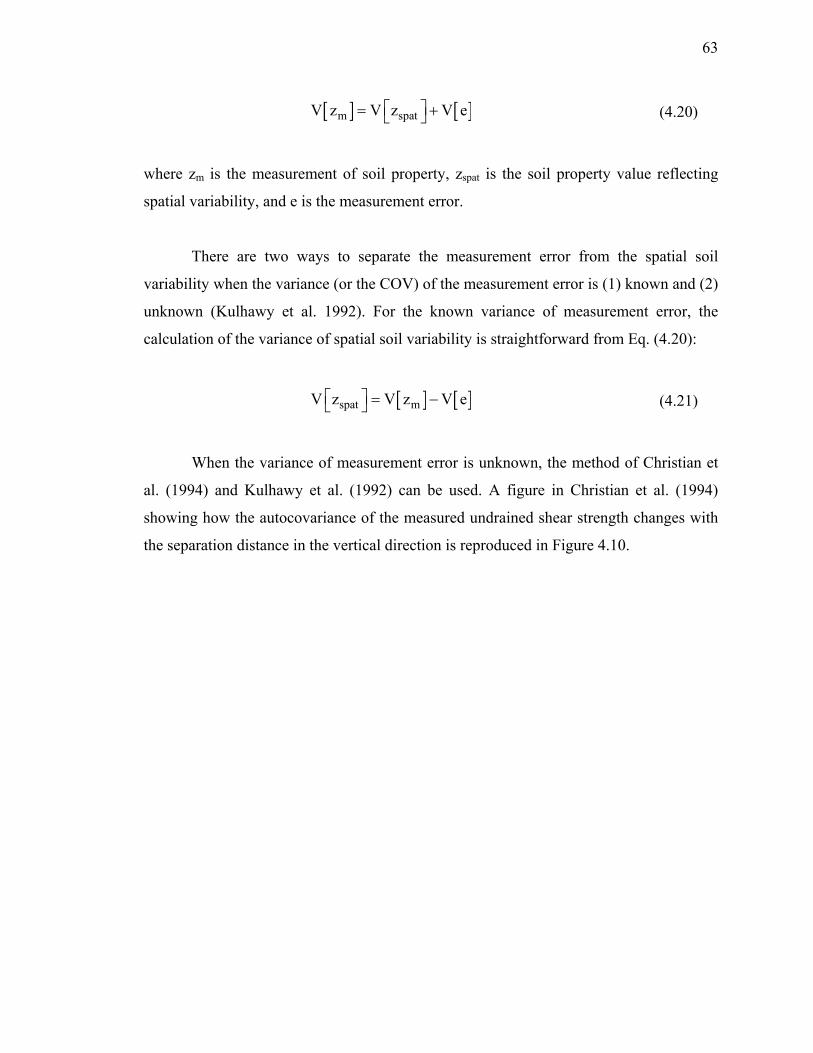
63
[ ] [ ]m spatV z V z V e⎡ ⎤= +⎣ ⎦ (4.20)
where zm is the measurement of soil property, zspat is the soil property value reflecting
spatial variability, and e is the measurement error.
There are two ways to separate the measurement error from the spatial soil
variability when the variance (or the COV) of the measurement error is (1) known and (2)
unknown (Kulhawy et al. 1992). For the known variance of measurement error, the
calculation of the variance of spatial soil variability is straightforward from Eq. (4.20):
[ ] [ ]spat mV z V z V e⎡ ⎤ = −⎣ ⎦ (4.21)
When the variance of measurement error is unknown, the method of Christian et
al. (1994) and Kulhawy et al. (1992) can be used. A figure in Christian et al. (1994)
showing how the autocovariance of the measured undrained shear strength changes with
the separation distance in the vertical direction is reproduced in Figure 4.10.
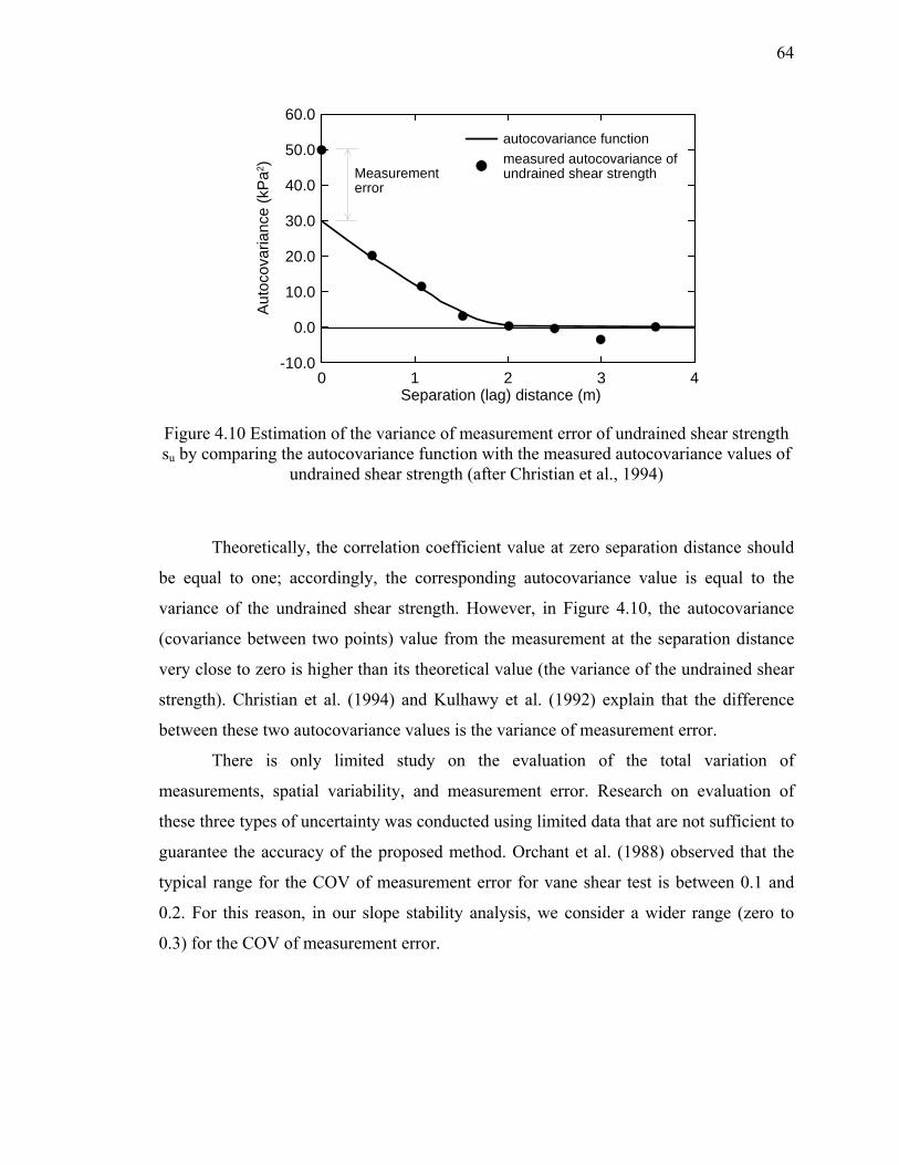
64
0 1 2 3 4Separation (lag) distance (m)
-10.0
0.0
10.0
20.0
30.0
40.0
50.0
60.0
Aut
ocov
aria
nce
(kP
a2 ) measured autocovariance ofundrained shear strength
autocovariance function
Measurementerror
Figure 4.10 Estimation of the variance of measurement error of undrained shear strength su by comparing the autocovariance function with the measured autocovariance values of
undrained shear strength (after Christian et al., 1994)
Theoretically, the correlation coefficient value at zero separation distance should
be equal to one; accordingly, the corresponding autocovariance value is equal to the
variance of the undrained shear strength. However, in Figure 4.10, the autocovariance
(covariance between two points) value from the measurement at the separation distance
very close to zero is higher than its theoretical value (the variance of the undrained shear
strength). Christian et al. (1994) and Kulhawy et al. (1992) explain that the difference
between these two autocovariance values is the variance of measurement error.
There is only limited study on the evaluation of the total variation of
measurements, spatial variability, and measurement error. Research on evaluation of
these three types of uncertainty was conducted using limited data that are not sufficient to
guarantee the accuracy of the proposed method. Orchant et al. (1988) observed that the
typical range for the COV of measurement error for vane shear test is between 0.1 and
0.2. For this reason, in our slope stability analysis, we consider a wider range (zero to
0.3) for the COV of measurement error.

65
4.5. Use of Fourier Transforms to Generate Gaussian Random Fields
A Gaussian random field of a soil property for a statistically homogeneous soil layer is
fully defined by the following components: (1) mean; (2) variation (or COV); (3)
correlation coefficient function; and (4) scale of fluctuation.
Generation of a Gaussian random field that reflects the mean and standard
deviation of the soil property could be done as follows: (1) select appropriate correlation
coefficient function and scale of fluctuation that reproduces the spatial soil variability of
the field; (2) generate a Gaussian random field that has zero mean and a standard
deviation of one using the correlation coefficient function and scale of fluctuation; (3)
multiply the standard deviation of the soil property by every value in the Gaussian
random field that is generated in the previous step; (4) add the mean value of the soil
property to each value of the Gaussian random field.
Fenton (1990) proposed a method for the generation of a Gaussian random field
using Fourier transforms. The two-dimensional discrete Fourier transform of the real
process written in terms of angular frequency is
( ) ( )
( ) ( )1 2
1 2
1 2
1 2
K 1 K 1
m 0 n 0
K 1 K 1
m 0 n 0
ij i j
mn x,m y,n mn x,m y,nK K
mn mn1 2 1 2K K
z z x , y z i x, j y
A cos i x j y B sin i x j y
2 im 2 jn 2 im 2 jnA cos B sinK K K K
lim lim
lim lim
− −
= =
− −
= =
→∞ →∞
→∞ →∞
= = Δ Δ
⎡= Δ ω + Δ ω + Δ ω + Δ ω⎣
⎡ ⎤⎛ ⎞ ⎛ ⎞π π π π= + + +⎢ ⎥⎜ ⎟ ⎜ ⎟
⎢ ⎥⎝ ⎠ ⎝ ⎠⎣ ⎦
∑ ∑
∑ ∑
(4.22)
where Δx and Δy are the discretization intervals in the x and y directions, K1 and K2 are
the discretization elements in the x and y direction, Amn and Bmn are the independent
Fourier coefficients that follow a normal distribution with zero mean, xi and yj are the
physical lengths from zero to the end of the ith and jth interval in the x and y directions,
and ωx,m (=2mπ/K1Δx) and ωy,n ( =2nπ/K2Δy ) are the angular frequencies of the Fourier
series in the x and y directions.

66
Because Gaussian random fields used in slope stability analysis have a finite
number of discretization elements in the x and y direction, zij can be represented as:
1 2K 1K 1
ij mn mn1 2 1 2m 0 n 0
2 im 2 jn 2 im 2 jnz A cos B sinK K K K
− −
= =
⎡ ⎤⎛ ⎞ ⎛ ⎞π π π π= + + +⎢ ⎥⎜ ⎟ ⎜ ⎟
⎝ ⎠ ⎝ ⎠⎣ ⎦∑ ∑ (4.23)
Then, the Fourier coefficients Amn and Bmn (derivation of the Fourier coefficients
is provided in Appendix C) in Eq. (4.23) are
1 2K 1K 1
mn ij1 2 1 2i 0 j 0
1 2 im 2 jnA z cosK K K K
− −
= =
⎛ ⎞π π= +⎜ ⎟
⎝ ⎠∑ ∑ (4.24)
1 2K 1K 1
mn ij1 2 1 2i 0 j 0
1 2 im 2 jnB z sinK K K K
− −
= =
⎛ ⎞π π= +⎜ ⎟
⎝ ⎠∑ ∑ (4.25)
Because the expected value of zij is zero for any points (xi,yj) in the random field,
the expected values of Amn and Bmn must be zero; therefore, the variances of Amn and Bmn
are equal to the expected values of the squares of Amn and Bmn, respectively:
[ ]
( )
1 2 1 2
2mn mn
ij klK 1K 1K 1K 1
2i 0 j 0 k 0 l 01 2
1 2 1 2
V A E A
E z z1
2 im 2 jn 2 km 2 lncos cosK KK K K K
− − − −
= = = =
⎡ ⎤= ⎣ ⎦⎧ ⎫⎡ ⎤ ×⎣ ⎦⎪ ⎪⎪ ⎪= ⎨ ⎬⎛ ⎞ ⎛ ⎞π π π π
+ +⎪ ⎪⎜ ⎟ ⎜ ⎟⎪ ⎪⎝ ⎠ ⎝ ⎠⎩ ⎭
∑ ∑ ∑ ∑ (4.26)
[ ]
( )
1 2 1 2
2mn mn
ij klK 1K 1K 1K 1
2i 0 j 0 k 0 l 01 2
1 2 1 2
V B E B
E z z1
2 im 2 jn 2 km 2 lnsin sinK KK K K K
− − − −
= = = =
⎡ ⎤= ⎣ ⎦⎧ ⎫⎡ ⎤ ×⎣ ⎦⎪ ⎪⎪ ⎪= ⎨ ⎬⎛ ⎞ ⎛ ⎞π π π π
+ +⎪ ⎪⎜ ⎟ ⎜ ⎟⎪ ⎪⎝ ⎠ ⎝ ⎠⎩ ⎭
∑ ∑ ∑ ∑ (4.27)

67
The calculation of the variances of Amn and Bmn can be approximated using the
spectral density function S of the process zij. The spectral density function represents the
strength of the variations in terms of frequency. For example, when the spectral density
function has a high value at a certain frequency, it means the variation at that frequency is
strong. The integration of the spectral density function within a specific frequency range
renders the strength of variation within that frequency range. From Wiener-Chintchin
relationship, the relationship between spectral density function S and the correlation
coefficient function ρ for the Gaussian random field is
( ) ( ) ( )x y x y x yx, y S , cos x y d d∞ ∞
−∞ −∞ρ = ω ω ω + ω ω ω∫ ∫ (4.28)
where x and y are the separation distances in the horizontal and vertical directions,
respectively.
Using the relationship that cos(α+β) = cos(α) cos(β) - sin(α) sin(β), Eq. (4.28)
can be modified as
( )( )
( ) ( ) ( ) ( )x y
x yx y x y
S ,x, y d d
cos x cos y sin x sin y
∞ ∞
−∞ −∞
⎧ ⎫ω ω⎪ ⎪ρ = ω ω⎨ ⎬⎡ ⎤× ω ω − ω ω⎪ ⎪⎣ ⎦⎩ ⎭
∫ ∫ (4.29)
Because the spectral density function S is even function with respect to each
direction x and y, Eq. (4.29) can be revised as
( ) ( ) ( ) ( )2x y x y x y0 0
x, y 2 S , cos x cos y d d∞ ∞
ρ = ω ω ω ω ω ω∫ ∫ (4.30)
By defining the one-sided spectral density function G as

68
( ) ( )2x y x yG , 2 S ,ω ω = ω ω (4.31)
Eq. (4.30) can be revised as
( ) ( ) ( ) ( )x y x y x y0 0x, y G , cos x cos y d d
∞ ∞ρ = ω ω ω ω ω ω∫ ∫ (4.32)
For the Gaussian random field that has zero mean and standard deviation of one,
the correlation coefficient function of the process zij can be represented as
( ) ( ) ( )z x y x yx, y E z , z x, y⎡ ⎤ρ = ξ ξ ξ + ξ +⎣ ⎦ (4.33)
where ξx and ξy are the random variables in x and y directions.
Suppose that the separation distances in the horizontal and vertical directions are
x = |i−k|Δx and y = |j−l|Δy, respectively. From Eq. (4.30) and Eq. (4.33), the correlation
coefficient function ρz of the process zij can be written in terms of the spectral density
function Gz:
( ) ( )
( ) ( ) ( )1 2
z z
K 1K 1
ij kl x y z x,m y,n1 1m 0 n 0
x, y i k x, j k y
2 m i k 2 n j lE z z G , cos cos
K K
− −
= =
ρ = ρ − Δ − Δ =
π − π −⎛ ⎞ ⎛ ⎞⎡ ⎤ ≈ Δω Δω ω ω ⎜ ⎟ ⎜ ⎟⎣ ⎦
⎝ ⎠ ⎝ ⎠∑ ∑
(4.34)
From the Wiener-Khinchin relationship, the spectral density function Gz for the
correlation coefficient function ρz(x,y) (Eq. (4.7)) is
( ) ( ) ( )2
z x,m y,n z x,m y,n0 01G , x, y cos x y dx dy
∞ ∞⎛ ⎞ω ω = ρ ω + ω⎜ ⎟π⎝ ⎠ ∫ ∫ (4.35)

69
The integration of Eq. (4.35) reveals (Fenton, 1990)
( )( )( )
2f
z x,m y,n 1.52 2 2f x,m y,n
4sG ,4 s
ω ω =π + ω + ω
(4.36)
By inserting Eq. (4.34) into Eq. (4.26) and Eq. (4.27), the variances of Amn and
Bmn are summarized as follows (Fenton, 1990):
[ ]
( )
( ) ( ){ }
( ) ( ){ }
( ) ( )( ) ( )
2
1
2
1 1 2
z x,m y,n x y 1 2
z x,m y,n z x,m y,K n x y 1
mnz x,m y,n z x,K m y,n x y 2
z x,m y,n z x,m y,K n
z x,K m y,n z x,K m y,K n
1 G , if m 0,K / 2 and n 0,K / 24
1 G , G , if m 0,K / 216
1V A G , G , if n 0,K / 216
G , G ,132 G , G ,
−
−
−
− − −
ω ω Δω Δω = =
ω ω + ω ω Δω Δω =
= ω ω + ω ω Δω Δω =
⎧ ω ω + ω ω⎪⎨
+ ω ω + ω ωx y otherwise
⎧⎪⎪⎪⎪⎪⎪⎪⎪⎨⎪⎪⎪⎪ ⎫⎪ ⎪Δω Δω⎬⎪
⎪ ⎪⎪ ⎩ ⎭⎪⎩
(4.37)
[ ]
( ) ( ){ }
( ) ( ){ }
( ) ( )( ) ( )
2
1
2
1 1 2
1 2
z x,m y,n z x,m y,K n x y 1
mn z x,m y,n z x,K m y,n x y 2
z x,m y,n z x,m y,K nx y
z x,K m y,n z x,K m y,K n
0 if m 0,K / 2 and n 0,K / 2
1 G , G , if m 0,K / 216
1V B G , G , if n 0,K / 216
G , G ,1 other32 G , G ,
−
−
−
− − −
= =
ω ω + ω ω Δω Δω =
= ω ω + ω ω Δω Δω =
⎧ ⎫ω ω + ω ω⎪ ⎪Δω Δω⎨ ⎬+ ω ω + ω ω⎪ ⎪⎩ ⎭
wise
⎧⎪⎪⎪⎪⎪⎪⎪⎪⎨⎪⎪⎪⎪⎪⎪⎪⎪⎩
(4.38)

70
4.6. Procedure for Gaussian Random Field Generation
The following are the steps for the generation of a two-dimensional Gaussian
random field using Fourier transforms (Fenton, 1990):
1. Suppose the area for which we will use a Gaussian random field theory to
represent a specific soil property has dimensions L1 × L2 (L1 and L2 are the
lengths in the horizontal and vertical directions, respectively). In this case, we
need to generate a Gaussian random field for which the lengths in each direction
(D1 and D2 for the horizontal and vertical directions respectively) are twice the
required lengths (D1=2L1 and D2=2L2). The excess lengths will be disregard in the
final step (Fenton, 1994);
2. Divide the lengths of the horizontal and vertical directions (D1 and D2) into small
intervals;
3. Calculate the variances of Amn and Bmn for m = 0, 1,⋅⋅⋅, K1-1 and n = 0, 1,⋅⋅⋅, K2-1
using Eq. (4.37) and Eq. (4.38);
4. Generate random numbers for Amn and Bmn (for m = 0, 1, ⋅⋅⋅ , K1-1 and n = 0, 1, ⋅⋅⋅
, K2-1) based on the assumptions that Amn and Bmn follow normal distributions
with zero mean and the variance determined in the previous step (step 3);.
5. Generate the values of the random variable z(xi,xj)real for all the discretization
points for the required domain (L1 × L2) by inputting Amn and Bmn values into Eq.
(4.23);
6. Multiply the z(xi,xj)real values by the standard deviation of the soil property and
add its mean value to them for the representation of the soil property.
Using this procedure, we generated two-dimensional Gaussian random fields that
have zero mean and unit standard deviation for different scales of fluctuation (sf=1, 5, 10,
and 20), as shown in Figure 4.11. For each scale of fluctuation, Figure 4.11 shows the
horizontal and tilted (15 degrees from the horizontal) views of the surface map of the
Gaussian random field.

71
Figure 4.11 Horizontal and tilted views of surface map of two-dimensional Gaussian random fields that has zero mean and unit standard deviation for different scales of
fluctuation; (a) sf = 1m, (b) sf = 5m, (c) sf = 10m, and (d) sf = 20m

72
CHAPTER 5. EXAMPLES OF RESISTANCE FACTOR CALCULATION
In this chapter, a series of slope stability analyses were performed using Monte Carlo
simulations to examine the effect of the scale of fluctuation and the uncertainty level of
measurement error on the probability of failure of the slope. In addition, examples are
given to show how to determine optimum factors (both optimum load and resistance
factors) for LRFD of slopes.
5.1. Effect of the Measurement Error on the Probability of Failure
To examine the effect of the measurement error on the probability of failure of slopes,
sets of reliability analyses were performed for the slope given in Figure 5.1, varying the
COV of measurement error. We assumed that the mean values for apparent cohesion c,
friction angle φ and soil unit weight γ of each soil layer are the values shown in Figure
5.1. The COVs for the spatial variabilities of c, φ, and γ that are used for this analysis are
taken as 0.2, 0.2, and 0.05, respectively. The scales of fluctuation for the parameters c, φ,
and γ are assumed as 10m. The COV and scale of fluctuation values for these soil
parameters are selected for the purpose of examining the effect of the measurement error
on the probability of failure. These values are different from the values that we are using
for the development of LRFD for slopes.
73
Layer 1
Layer 2
Layer 3
c1=6 kPa, φ1=2°, γ1=18 kN/m3
c2=5 kPa, φ2=25°, γ2=19 kN/m3
c3=6 kPa, φ3=11°, γ3=19.5 kN/m3 20m
Slope angle=30°Slope height=5.774m
2.887m
2.887m
10m
Figure 5.1 Geometry of a three-layer soil slope and its soil properties
Different levels of the COV of measurement error are selected (0, 0.1, 0.2, and
0.3) to assess its effect on the probability of failure of the given slope. For each level of
the COV of measurement, the computed probability of failure using Monte Carlo
simulation with 10,000 realizations (or FS calculations) varied from simulation to
simulation within a narrow range. To overcome this convergence issue, a large number of
realizations are required. We tried to determine the minimum number of realizations that
would produce a converging (or consistent) probability of failure. From Figure 5.2, we
had a fairly consistent probability of failure after 30,000 realizations. Accordingly, we
conducted more than 30,000 realizations in Monte Carlo simulation for every probability
of failure calculation.
As shown in Figure 5.2, we found that an increase in the COV of the
measurement error does not have a significant effect on probability of failure. If the
method of slices is used for slope stability analysis, distribution of the measurement error
at each slice has zero mean following a normal distribution; therefore, the probability that
the measurement error of soil property will increase the stability of a slope is equal to the
probability that it will decrease the stability of the slope. For a large number of slices this
means that the change in probability of failure due to the measurement error is not
significant.

74
0 20000 40000 60000 80000 100000Number of realizations
0.000
0.004
0.008
0.012
0.016
0.020
Prob
abili
ty o
f fai
lure
COVmeas. = 0.0COVmeas. = 0.1COVmeas. = 0.2COVmeas. = 0.3
Figure 5.2 Effect of the COV of measurement on a probability of failure of the slope given in Figure 5.1
5.2. Effect of the Isotropic Scale of Fluctuation of Soil Unit Weight on the Probability of Failure
As mentioned in chapter 4, due to the scarcity of published research performed on the
isotropic scale of fluctuation sf of soil unit weight, we conducted sets of reliability
analyses for the slope given in Figure 5.1 to examine the effect of the isotropic scale of
fluctuation of soil unit weight on the probability of failure of the slope, fixing the sf
values of strength parameters equal to 10m and varying the sf of soil unit weight (sf =1, 5,
10, and 20m). We assumed that the mean values and COVs for spatial variabilities of the
parameters (c, φ, and γ) used for this analysis are the same as those used in the example in
the previous section (section 5.1).
The probabilities of failure calculated for the slope in Figure 5.1 for different
values of sf (sf=1, 5, 10, and 20m) of soil unit weight are represented in Figure 5.3. The
probability of failure ranged from 0.0042 to 0.0049 with an average of 0.0046. Even
though we observe some difference in probability of failure with respect to the value of
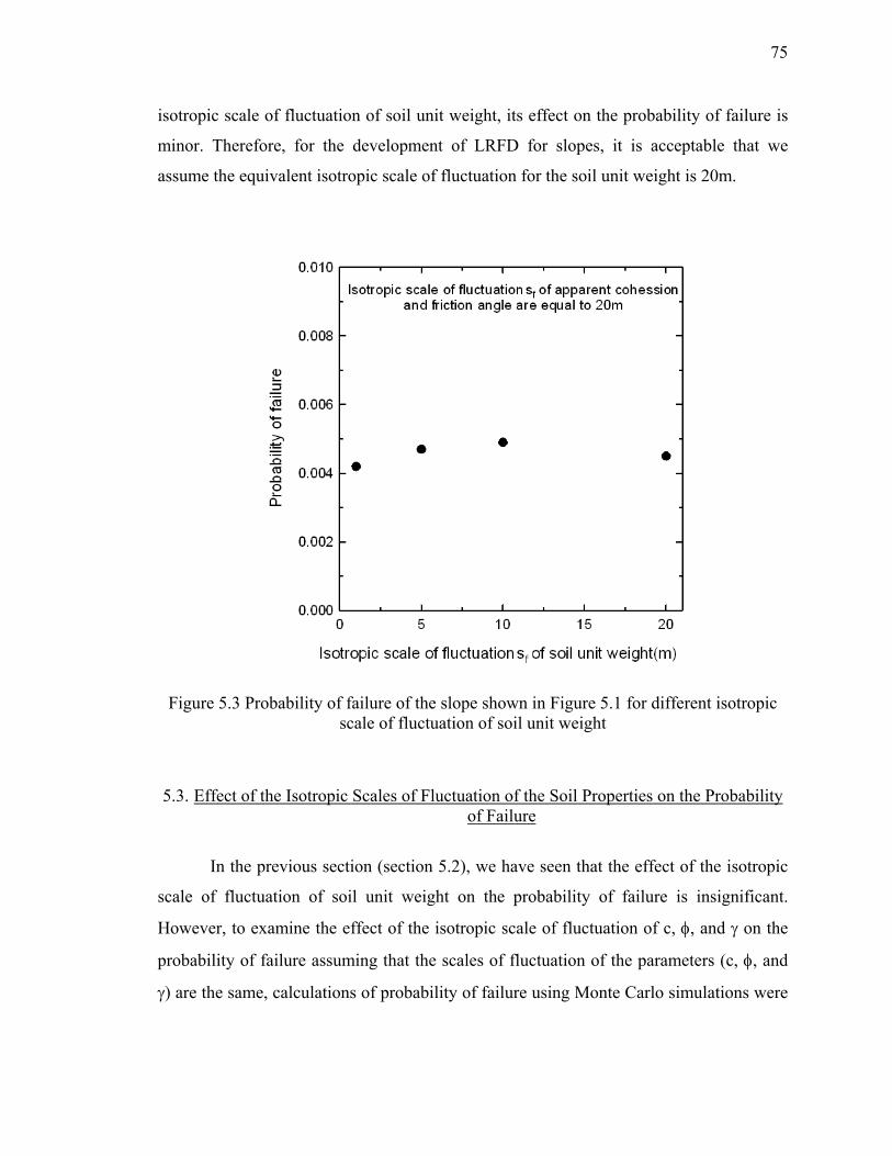
75
isotropic scale of fluctuation of soil unit weight, its effect on the probability of failure is
minor. Therefore, for the development of LRFD for slopes, it is acceptable that we
assume the equivalent isotropic scale of fluctuation for the soil unit weight is 20m.
Figure 5.3 Probability of failure of the slope shown in Figure 5.1 for different isotropic scale of fluctuation of soil unit weight
5.3. Effect of the Isotropic Scales of Fluctuation of the Soil Properties on the Probability of Failure
In the previous section (section 5.2), we have seen that the effect of the isotropic
scale of fluctuation of soil unit weight on the probability of failure is insignificant.
However, to examine the effect of the isotropic scale of fluctuation of c, φ, and γ on the
probability of failure assuming that the scales of fluctuation of the parameters (c, φ, and
γ) are the same, calculations of probability of failure using Monte Carlo simulations were
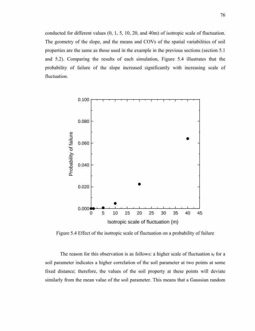
76
conducted for different values (0, 1, 5, 10, 20, and 40m) of isotropic scale of fluctuation.
The geometry of the slope, and the means and COVs of the spatial variabilities of soil
properties are the same as those used in the example in the previous sections (section 5.1
and 5.2). Comparing the results of each simulation, Figure 5.4 illustrates that the
probability of failure of the slope increased significantly with increasing scale of
fluctuation.
0 5 10 15 20 25 30 35 40 45
Isotropic scale of fluctuation (m)
0.000
0.020
0.040
0.060
0.080
0.100
Pro
babi
lity
of fa
ilure
Figure 5.4 Effect of the isotropic scale of fluctuation on a probability of failure
The reason for this observation is as follows: a higher scale of fluctuation sf for a
soil parameter indicates a higher correlation of the soil parameter at two points at some
fixed distance; therefore, the values of the soil property at these points will deviate
similarly from the mean value of the soil parameter. This means that a Gaussian random

77
field with a higher sf may result significantly weaker across the entire slope or large parts
of it more often, which in turn leads to lower probability of failure.
5.4. Examples for Slopes and Embankments
In this section, the optimum resistance and load factors are calculated following the
algorithm shown in Figure 3.3. Two different target probabilities of failure Pf are
considered (Pf = 0.001 and 0.01). Even though the suggestion of COV values for apparent
cohesion and friction angle is not advisable, the COV values for apparent cohesion,
friction angle, and soil unit weight are assumed as 0.4, 0.4, 0.2, and 0.1, respectively, for
the purpose of developing LRFD for slopes. The isotropic scales of fluctuation for the
soil parameters (c, φ, and γ) are taken as 20m, as mentioned in the previous chapter.
5.4.1. Slope example 1: Pf = 0.001, no live uniform surcharge load on the crest of the slope
The algorithm for LRFD of slopes shown in Figure 3.3 is used for a slope with the
geometry of Figure 5.5. In the analysis, 30,000 realizations (or FS calculations) were
done, each for one combination of random fields for all the soil parameters of every soil
layer, and the results were used for each calculation of the probability of failure for the
slope.

78
Layer 1
Layer 2
Layer 3
c1, φ1, γ1
c2, φ2, γ2
c3, φ3, γ3
2.887m
2.887m
10m
Slope angle=30°Slope height=5.774m
Figure 5.5 Geometry of a three-layer soil slope
To find the combination of the expect values of the soil parameters (c, φ, and γ) of
each layer that produce the target probability of failure (Pf = 0.001), the initial guess for
the soil parameters was as follow: (1) layer 1: c1 = 5 kPa, φ1 = 10°, γ1 =18 kN/m3; (2)
layer 2: c2 = 2 kPa, φ2 = 25°, γ2 =19 kN/m3; and (3) layer 3: c3 = 10 kPa, φ3 = 15°, γ3
=19.5 kN/m3. The calculated probability of failure in this case was 0.0031. By changing
these expected values, we found the expected values of the soil parameters that produced
the target probability of failure (0.001): (1) layer 1: c1 = 11.2 kPa, φ1 = 10°, γ1 =18
kN/m3; (2) layer 2: c2 = 5 kPa, φ2 = 20°, γ2 =19 kN/m3; and (3) layer 3: c3 = 10 kPa, φ3 =
20°, γ3 =19.5 kN/m3.
Due to the absence of external loads, the driving moment was induced only by the
self-weight of the soil. Therefore, only one optimum load factor exists in this example.
For a given slip surface, if the soil strengths have friction angle components, the soil self-
weights within the potential sliding mass influence both the driving and resisting
moments. For example, the soil self-weight of the potential sliding mass increases both
the driving and resisting moments. Therefore, the driving moment and resisting moment
are correlated. However, if the soil strengths only result from cohesion (with φ = 0), the
self-weight of the soil within the potential sliding mass affects only the driving moment,
not the resisting moment.

79
The distribution of the FS is shown in Figure 5.6. This distribution matches well
with a normal distribution. The probability of failure is very close to the target probability
of failure of 0.001 (29 failure cases out of 30,000 realizations). In the program, the
driving and resisting moments are normalized with respect to the corresponding radius of
the circular slip surface. This normalization has no influence on the FS calculation. The
ULS corresponds to the case that is equal to or closest to FS of one (FS=1); for this
particular Monte Carlo simulation, the ULS values of the driving and resisting moments
divided by the radius of the circular slip surface rslip are 145.392 and 145.382 kNm/m/m
respectively.
0.9 1 1.1 1.2 1.3 1.4 1.5 1.6 1.7 1.8 1.9Factor of safety
0
500
1000
1500
2000
2500
3000
Freq
uenc
y
Limit state(FS=1)
Mean = 1.383Standard deviation = 0.125
Probability of failurePf=0.001
From deterministic analysis,FS=1.324
Figure 5.6 Distribution of FS value and the ULS of the slope (Pf = 0.001 and without live uniform surcharge load)
For the calculation of nominal values of the driving and resisting moments, a
conventional (deterministic) slope stability analysis was performed using the nominal
values of the soil parameters and geometry of the slope. For the soil parameters c, φ, and
γ, in these analysis, the bias factors are equal to one; therefore, the nominal values of
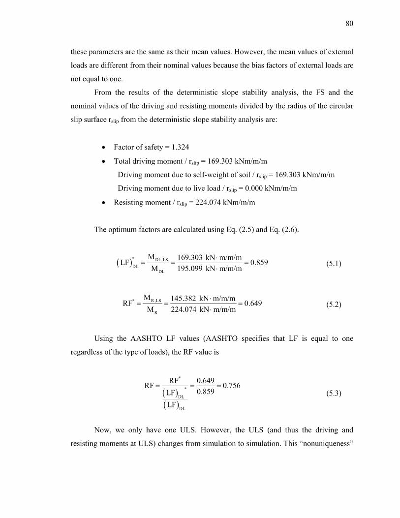
80
these parameters are the same as their mean values. However, the mean values of external
loads are different from their nominal values because the bias factors of external loads are
not equal to one.
From the results of the deterministic slope stability analysis, the FS and the
nominal values of the driving and resisting moments divided by the radius of the circular
slip surface rslip from the deterministic slope stability analysis are:
• Factor of safety = 1.324
• Total driving moment / rslip = 169.303 kNm/m/m
Driving moment due to self-weight of soil / rslip = 169.303 kNm/m/m
Driving moment due to live load / rslip = 0.000 kNm/m/m
• Resisting moment / rslip = 224.074 kNm/m/m
The optimum factors are calculated using Eq. (2.5) and Eq. (2.6).
( )* DL,LSDL
DL
M 169.303 kN m/m/mLF 0.859M 195.099 kN m/m/m
⋅= = =
⋅ (5.1)
R,LS*
R
M 145.382 kN m/m/mRF 0.649M 224.074 kN m/m/m
⋅= = =
⋅ (5.2)
Using the AASHTO LF values (AASHTO specifies that LF is equal to one
regardless of the type of loads), the RF value is
( )( )
*
*
DL
DL
RF 0.649RF 0.7560.859LF
LF
= = = (5.3)
Now, we only have one ULS. However, the ULS (and thus the driving and
resisting moments at ULS) changes from simulation to simulation. This “nonuniqueness”
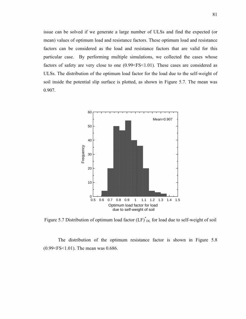
81
issue can be solved if we generate a large number of ULSs and find the expected (or
mean) values of optimum load and resistance factors. These optimum load and resistance
factors can be considered as the load and resistance factors that are valid for this
particular case. By performing multiple simulations, we collected the cases whose
factors of safety are very close to one (0.99<FS<1.01). These cases are considered as
ULSs. The distribution of the optimum load factor for the load due to the self-weight of
soil inside the potential slip surface is plotted, as shown in Figure 5.7. The mean was
0.907.
0.5 0.6 0.7 0.8 0.9 1 1.1 1.2 1.3 1.4 1.5Optimum load factor for load
due to self-weight of soil
0
10
20
30
40
50
60
Freq
uenc
y
Mean=0.907
Figure 5.7 Distribution of optimum load factor (LF)*DL for load due to self-weight of soil
The distribution of the optimum resistance factor is shown in Figure 5.8
(0.99<FS<1.01). The mean was 0.686.

82
0.3 0.4 0.5 0.6 0.7 0.8 0.9 1 1.1 1.2Optimum resistance factor
0
10
20
30
40
50
60
70
Freq
uenc
y
Mean=0.686
Figure 5.8 Distribution of optimum resistance factor RF*
If we use these mean values for the load and resistance factors, the factored load
and the factored resistance are:
i i(LF) Q 0.907 169.303 153.558kN m/m/m= × =∑ (5.4)
n(RF) R 0.686 224.074 154.715kN m/m/m= × = (5.5)
Therefore, the LRFD criterion [inequality (2.2)] is satisfied:
[ ] [ ]n i i(RF) R 154.715kN m/m/m (LF) Q 153.558kN m/m/m= ≥ =∑ (5.6)
Finding a large number of ULSs for each example takes considerable time.
Generating sufficient ULSs to have appropriate expected values of optimum factors is

83
important for the determination of the LFs and RF that we could propose for any slope
design.
5.4.2. Slope example 2: Pf = 0.01, no live uniform surcharge load on the crest of the slope
Monte Carlo simulations are conducted for the slope with the same geometry as that used
in example 1. By adjusting the expected values of soil parameters, we found that the
following expected values of the soil parameters produced the target probability of failure
(Pf = 0.01): (1) layer 1: c1 = 5 kPa, φ1 = 10°, γ1 =18 kN/m3; (2) layer 2: c2 = 5 kPa, φ2 =
23.7°, γ2 =19 kN/m3; and (3) layer 3: c3 = 10 kPa, φ3 = 10°, γ3 =19.5 kN/m3. The
probability of failure was calculated as 0.010 (299 failure cases out of 30,000 realizations.
Figure 5.9 represents the distribution of the FS from the analysis. Similar to the
previous example, the distribution of the FS value is close to a normal distribution. The
ULS values of the driving and resisting moments divided by rslip are 179.990 kNm/m/m
and 179.954 kNm/m/m.

84
0.9 1 1.1 1.2 1.3 1.4 1.5 1.6 1.7Factor of safety
0
500
1000
1500
2000
2500
3000
3500
Freq
uenc
y
Limit state(FS=1)
Mean = 1.231Standard deviation = 0.101
Probability of failurePf=0.01
From deterministic analysis,FS=1.284
Figure 5.9 Distribution of FS value and the ULS of the slope (Pf = 0.01, no live uniform surcharge load)
The results of deterministic analysis provide FS value and the nominal values of
the driving and resisting moments:
• Factor of safety = 1.284
• Total driving moment / rslip = 259.692 kNm/m/m
Driving moment due to self-weight of soil / rslip = 259.692 kNm/m/m
Driving moment due to live load / rslip = 0.000 kNm/m/m
• Resisting moment / rslip = 333.352 kNm/m/m
Therefore, the optimum factors can be obtained as
( )* DL,LSDL
DL
M 179.990 kN m/m/mLF 0.693M 256.692 kN m/m/m
⋅= = =
⋅ (5.7)

85
R,LS*
R
M 179.954 kN m/m/mRF 0.540M 333.352 kN m/m/m
⋅= = =
⋅ (5.8)
Using the AASHTO LF values (LF=1 regardless of the type of loads), the RF
value is
( )( )
*
*
DL
DL
RF 0.540RF 0.7790.693LF
LF
= = = (5.9)
Similarly to the previous example, we collected the cases whose factors of safety
are very close to one (0.99<FS<1.01). Figure 5.10 shows the distribution of the optimum
load factor for the load due to the self-weight of soil. The mean value of this optimum
load factor was 0.999.
0 0.2 0.4 0.6 0.8 1 1.2 1.4 1.6 1.8 2Optimum load factor for load
due to self-weight of soil
0
30
60
90
120
150
Freq
uenc
y
Mean=0.999
Figure 5.10 Distribution of optimum load factor (LF)*LD for load due to self-weight of
soil

86
Figure 5.11 represents the distribution of the optimum resistance factor
(0.99<FS<1.01). The mean value was 0.779.
0 0.2 0.4 0.6 0.8 1 1.2 1.4Optimum resistance factor
0
30
60
90
120
150
Freq
uenc
y
Mean=0.779
Figure 5.11 Distribution of optimum resistance factor RF*
If we use these mean values for the load and resistance factors, the factored load
and the factored resistance are:
i i(LF) Q 0.999 259.692 259.432 kN m/m/m= × =∑ (5.10)
n(RF) R 0.779 333.352 259.681kN m/m/m= × = (5.11)
The LRFD criterion [inequality (2.2)] is satisfied:
[ ] [ ]n i i(RF) R 259.681kN m/m/m (LF) Q 259.432 kN m/m/m= ≥ =∑ (5.12)
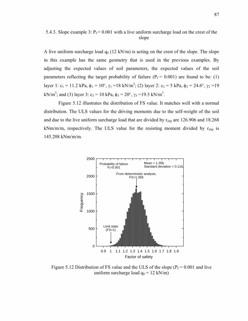
87
5.4.3. Slope example 3: Pf = 0.001 with a live uniform surcharge load on the crest of the slope
A live uniform surcharge load q0 (12 kN/m) is acting on the crest of the slope. The slope
in this example has the same geometry that is used in the previous examples. By
adjusting the expected values of soil parameters, the expected values of the soil
parameters reflecting the target probability of failure (Pf = 0.001) are found to be: (1)
layer 1: c1 = 11.2 kPa, φ1 = 10°, γ1 =18 kN/m3; (2) layer 2: c2 = 5 kPa, φ2 = 24.6°, γ2 =19
kN/m3; and (3) layer 3: c3 = 10 kPa, φ3 = 20°, γ3 =19.5 kN/m3.
Figure 5.12 illustrates the distribution of FS value. It matches well with a normal
distribution. The ULS values for the driving moments due to the self-weight of the soil
and due to the live uniform surcharge load that are divided by rslip are 126.906 and 18.268
kNm/m/m, respectively. The ULS value for the resisting moment divided by rslip is
145.208 kNm/m/m.
0.9 1 1.1 1.2 1.3 1.4 1.5 1.6 1.7 1.8 1.9Factor of safety
0
500
1000
1500
2000
2500
Freq
uenc
y
Limit state(FS=1)
Mean = 1.356Standard deviation = 0.116
Probability of failurePf=0.001
From deterministic analysis,FS=1.358
Figure 5.12 Distribution of FS value and the ULS of the slope (Pf = 0.001 and live uniform surcharge load q0 = 12 kN/m)
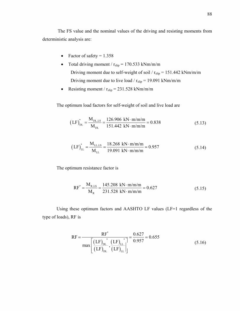
88
The FS value and the nominal values of the driving and resisting moments from
deterministic analysis are:
• Factor of safety = 1.358
• Total driving moment / rslip = 170.533 kNm/m/m
Driving moment due to self-weight of soil / rslip = 151.442 kNm/m/m
Driving moment due to live load / rslip = 19.091 kNm/m/m
• Resisting moment / rslip = 231.528 kNm/m/m
The optimum load factors for self-weight of soil and live load are
( )* DL,LSDL
DL
M 126.906 kN m/m/mLF 0.838M 151.442 kN m/m/m
⋅= = =
⋅ (5.13)
( )* LL,LSLL
LL
M 18.268 kN m/m/mLF 0.957M 19.091 kN m/m/m
⋅= = =
⋅ (5.14)
The optimum resistance factor is
R,LS*
R
M 145.208 kN m/m/mRF 0.627M 231.528 kN m/m/m
⋅= = =
⋅ (5.15)
Using these optimum factors and AASHTO LF values (LF=1 regardless of the
type of loads), RF is
( )( )
( )( )
*
* *
DL LL
DL LL
RF 0.627RF 0.6550.957LF LF
max ,LF LF
= = =⎡ ⎤⎢ ⎥⎢ ⎥⎣ ⎦
(5.16)

89
Figure 5.13 and Figure 5.14 show the distributions of the optimum load factor for
the load due to the self-weight of soil and that for the live surcharge load for the cases
whose factors of safety are very close to one (0.99<FS<1.01). The mean values of these
optimum load factors were 1.033 and 1.603, respectively.
0.6 0.7 0.8 0.9 1 1.1 1.2 1.3 1.4 1.5 1.6Optimum load factor for load
due to self-weight of soil
0
5
10
15
20
25
30
35
40
45
50Fr
eque
ncy
Mean=1.033(LF)*DL
Figure 5.13 Distribution of optimum load factor (LF)*DL for load due to self-weight of
soil

90
0 0.3 0.6 0.9 1.2 1.5 1.8 2.1 2.4 2.7 3 3.3Optimum load factor for load
due to live surcharge load
0
5
10
15
20
25
30
35
40
45
50
Freq
uenc
y
Mean=1.603(LF)*LL
Figure 5.14 Distribution of optimum load factor (LF)*LL for load due to live surcharge
load
Figure 5.15 represents the distribution of optimum resistance factor. The mean
value was 0.809.

91
0.3 0.4 0.5 0.6 0.7 0.8 0.9 1 1.1 1.2 1.3Optimum resistance factor
0
5
10
15
20
25
30
35
40
45
50
Freq
uenc
y
Mean=0.809RF*
Figure 5.15 Distribution of optimum resistance factor RF*
If we use these mean values for the load and resistance factors, the factored load
and the factored resistance are:
i i(LF) Q 1.033 151.442 1.603 30.603 187.043kN m/m/m= × + × =∑ (5.17)
n(RF) R 0.809 231.528 187.306kN m/m/m= × = (5.18)
The LRFD criterion [inequality (2.2)] is satisfied:
[ ] [ ]n i i(RF) R 187.306kN m/m/m (LF) Q 187.043kN m/m/m= ≥ =∑ (5.19)
92
5.4.4. Slope example 4: Pf = 0.01 with a live uniform surcharge load on the crest of the slope
The same magnitude of a live uniform surcharge load (q0 =12 kN/m) used in the previous
example is applied on the crest of the slope. By adjusting the expected values of soil
parameters, the expected values of the soil parameters that produce the target probability
of failure (Pf=0.01) are found to be: (1) layer 1: c1 = 11.2 kPa, φ1 = 10°, γ1 =18 kN/m3; (2)
layer 2: c2 = 5 kPa, φ2 = 21°, γ2 =19 kN/m3; and (3) layer 3: c3 = 10 kPa, φ3 = 20°, γ3
=19.5 kN/m3.
The distribution of FS is shown in Figure 5.16. The ULS values for the driving
moments due to the self-weight of the soil and due to the live uniform surcharge load that
are divided by rslip are 169.420 and 30.459 kNm/m/m, respectively. In addition, the ULS
value for the resisting moment divided by rslip is 199.855 kNm/m/m.
0.9 1 1.1 1.2 1.3 1.4 1.5 1.6 1.7 1.8Factor of safety
0
500
1000
1500
2000
2500
3000
Freq
uenc
y
Limit state(FS=1)
Mean = 1.259Standard deviation = 0.109
Probability of failurePf=0.01
From deterministic analysis,FS=1.243
Figure 5.16 Distribution of FS value and the ULS of the slope (Pf = 0.01 and live uniform surcharge load q0 = 12 kN/m)
93
The results of the deterministic analysis are summarized as:
• Factor of safety = 1.243
• Total driving moment / rslip = 204.841 kNm/m/m
Driving moment due to self-weight of soil / rslip = 179.469 kNm/m/m
Driving moment due to live load / rslip = 25.372 kNm/m/m
• Resisting moment / rslip = 254.624 kNm/m/m
The optimum values are
( )* DL,LSDL
DL
M 169.420 kN m/m/mLF 0.944M 179.469 kN m/m/m
⋅= = =
⋅ (5.20)
( )* LL,LSLL
LL
M 30.459 kN m/m/mLF 1.200M 25.372 kN m/m/m
⋅= = =
⋅ (5.21)
R,LS*
R
M 199.855 kN m/m/mRF 0.785M 254.624 kN m/m/m
⋅= = =
⋅ (5.22)
Using these optimum factors and AASHTO LF values (LF=1 regardless of the
type of loads), RF is
( )( )
( )( )
*
* *
DL LL
DL LL
RF 0.785RF 0.6541.200LF LF
max ,LF LF
= = =⎡ ⎤⎢ ⎥⎢ ⎥⎣ ⎦
(5.23)
Figure 5.17 and Figure 5.18 are the distributions of the optimum load factor for
the load due to the self-weight of soil and that for the live surcharge load for the cases
whose factors of safety are very close to one (0.99<FS<1.01). The mean values of these
optimum load factors were 0.897 and 1.188, respectively.

94
0.3 0.4 0.5 0.6 0.7 0.8 0.9 1 1.1 1.2 1.3 1.4 1.5Optimum load factor for load
due to self-weight of soil
0
30
60
90
120
150
Freq
uenc
y
Mean=0.897(LF)*DL
Figure 5.17 Distribution of optimum load factor (LF)*DL for load due to self-weight of
soil
0 0.5 1 1.5 2 2.5 3 3.5 4Optimum load factor for load
due to live surcharge load
0
30
60
90
120
150
Freq
uenc
y
Mean=1.188(LF)*LL
Figure 5.18 Distribution of optimum load factor (LF)*LL for load due to live surcharge
load

95
Figure 5.19 is the distribution of the optimum resistance factor. The mean value
was 0.752.
0.3 0.4 0.5 0.6 0.7 0.8 0.9 1 1.1 1.2 1.3 1.4 1.5Optimum resistance factor
0
30
60
90
120
150
Freq
uenc
y
Mean=0.752RF*
Figure 5.19 Distribution of optimum resistance factor RF*
If we use these mean values for the load and resistance factors, the factored load
and the factored resistance are:
i i(LF) Q 0.897 179.469 1.188 25.372 191.126 kN m/m/m= × + × =∑ (5.24)
n(RF) R 0.752 254.624 191.477 kN m/m/m= × = (5.25)
The LRFD criterion [inequality (2.2)] is satisfied:
[ ] [ ]n i i(RF) R 191.477kN m/m/m (LF) Q 191.126 kN m/m/m= ≥ =∑ (5.26)

96
5.4.5. Embankment example 1: Pf = 0.001
A road embankment in Figure 5.20 is used for this example. The road embankment has
side slopes at 1:1 and its height and width on the top are 5m and 10m, respectively.
Although, AASHTO and FHWA specifications propose the equivalent uniform surcharge
load to the vehicular load on the top of retaining structures, they do not provide the
equivalent uniform surcharge to the vehicular load for embankments. Therefore, to
account for the vehicular load acting on the top of the embankment, the equivalent live
uniform surcharge load is assumed as 12 kN/m.
0.4m
Layer 1: Sand 4.6m
5m 5m
Layer 2: Foundation soil
Pavement
5m
Figure 5.20 Geometry of a road embankment (1:1 side slopes)
The algorithm for LRFD of slopes shown in Figure 3.3 is used for the
development of LRFD for the side slopes of embankments. Because the thickness of the
pavement is relatively thin than that of soil layers composing the embankment, we
assumed that the strength parameters (c and φ) and the unit weight of pavement are the
same as those of sand. By adjusting the expected values of soil parameters, the expected
values of the soil parameters that produce the target probability of failure (Pf = 0.001) are
found to be: (1) layer 1: c1 = 6 kPa, φ1 = 36.25°, γ1 =20 kN/m3 and (2) layer 2: c2 = 5 kPa,
φ2 = 30°, γ2 =19 kN/m3.

97
The distribution of FS is shown in Figure 5.21. The ULS values for the driving
moments due to the self-weight of the soil and due to the live uniform surcharge load that
are divided by rslip are 92.825 and 14.115 kNm/m/m, respectively. In addition, the ULS
value for the resisting moment divided by rslip is 106.954 kNm/m/m.
0.9 1 1.1 1.2 1.3 1.4 1.5 1.6 1.7 1.8 1.9 2 2.1Factor of safety
0
1000
2000
3000
4000Fr
eque
ncy
Limit state(FS=1)
Mean = 1.483Standard deviation = 0.160
Probability of failurePf=0.001
From deterministic analysis,FS=1.429
Figure 5.21 Distribution of FS value and the ULS of the slope (Pf = 0.001 and live uniform surcharge load q0 = 12 kN/m)
The results of the deterministic analysis are summarized as:
Factor of safety = 1.429
• Total driving moment / rslip = 121.291 kNm/m/m
Driving moment due to self-weight of soil / rslip = 104.863 kNm/m/m
Driving moment due to live load / rslip = 16.428 kNm/m/m
• Resisting moment / rslip = 173.352 kNm/m/m
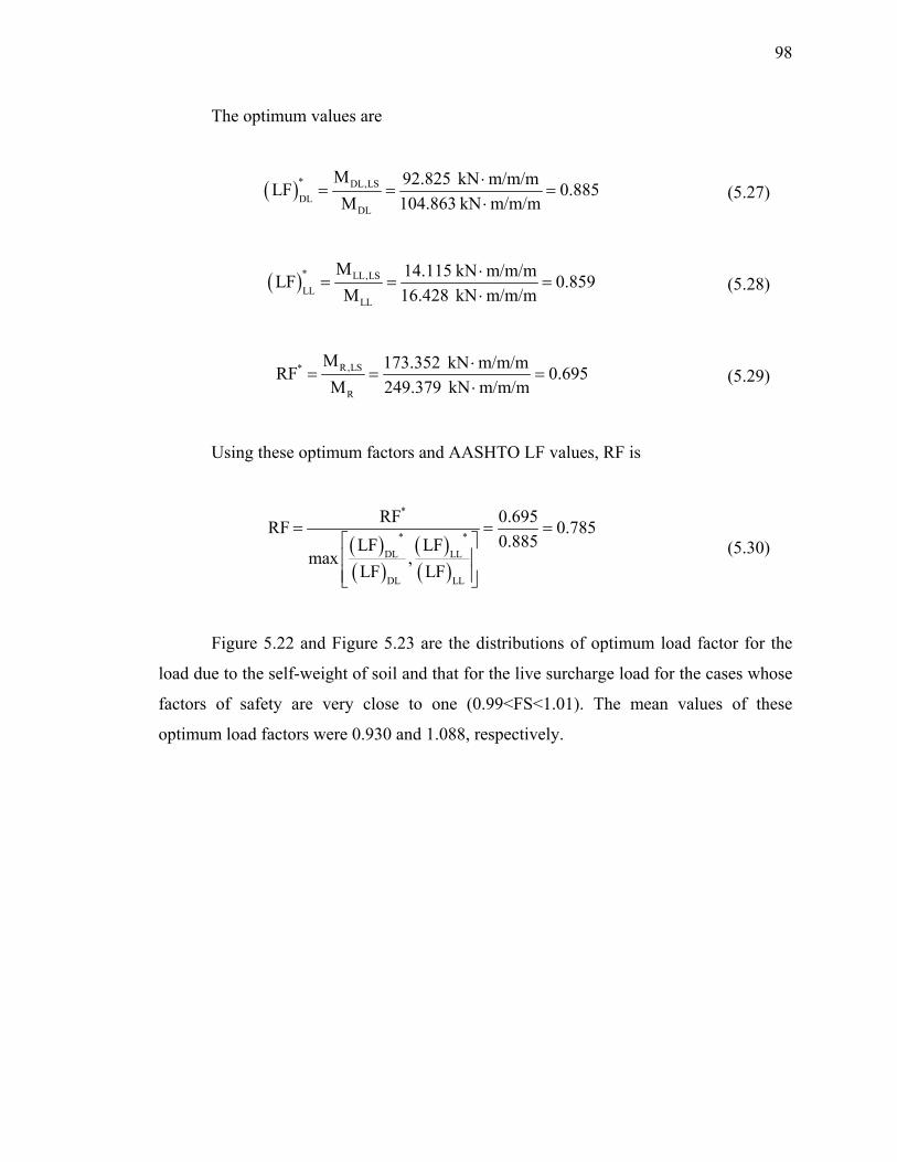
98
The optimum values are
( )* DL,LSDL
DL
M 92.825 kN m/m/mLF 0.885M 104.863 kN m/m/m
⋅= = =
⋅ (5.27)
( )* LL,LSLL
LL
M 14.115 kN m/m/mLF 0.859M 16.428 kN m/m/m
⋅= = =
⋅ (5.28)
R,LS*
R
M 173.352 kN m/m/mRF 0.695M 249.379 kN m/m/m
⋅= = =
⋅ (5.29)
Using these optimum factors and AASHTO LF values, RF is
( )( )
( )( )
*
* *
DL LL
DL LL
RF 0.695RF 0.7850.885LF LF
max ,LF LF
= = =⎡ ⎤⎢ ⎥⎢ ⎥⎣ ⎦
(5.30)
Figure 5.22 and Figure 5.23 are the distributions of optimum load factor for the
load due to the self-weight of soil and that for the live surcharge load for the cases whose
factors of safety are very close to one (0.99<FS<1.01). The mean values of these
optimum load factors were 0.930 and 1.088, respectively.

99
0.3 0.6 0.9 1.2 1.5 1.8Optimum load factor for load
due to self-weight of soil
0
5
10
15
20
25
30
35
40
45
50
Freq
uenc
y
Mean=0.930(LF)*DL
Figure 5.22 Distribution of optimum load factor (LF)*DL for load due to self-weight of
soil
0 0.4 0.8 1.2 1.6 2 2.4 2.8 3.2 3.6 4Optimum load factor for load
due to live surcharge load
0
5
10
15
20
25
30
35
40
45
50
Freq
uenc
y
Mean=1.088(LF)*LL
Figure 5.23 Distribution of optimum load factor (LF)*LL for load due to live surcharge
load

100
Figure 5.24 is the distribution of optimum resistance factor. The mean value was
0.666.
0 0.2 0.4 0.6 0.8 1 1.2 1.4Optimum resistance factor
0
5
10
15
20
25
30
35
40
45
50
55
60
Freq
uenc
y
Mean=0.666RF*
Figure 5.24 Distribution of optimum resistance factor RF*
If we use these mean values for load and resistance factor, the factored load and
the factored resistance are:
i i(LF) Q 0.930 104.863 1.088 16.428 115.396 kN m/m/m= × + × =∑ (5.31)
n(RF) R 0.666 173.352 115.452kN m/m/m= × = (5.32)
The LRFD criterion [inequality (2.2)] is satisfied:
[ ] [ ]n i i(RF) R 115.452kN m/m/m (LF) Q 115.396 kN m/m/m= ≥ =∑ (5.33)

101
5.4.6. Embankment example 2: Pf = 0.01
The same geometry of the slope in the previous example is used in this example with
different target probability of failure (Pf = 0.01). The design live uniform surcharge load
on the top of the embankment is also assumed as 12 kN/m. By adjusting expected values
of soil parameters, the expected values of the soil parameters that produce the target
probability of failure equal to 0.01 are found to be: (1) layer 1: c1 = 6 kPa, φ1 = 33°, γ1
=20 kN/m3 and (2) layer 2: c2 = 5 kPa, φ2 = 17.2°, γ2 =19 kN/m3.
The distribution of FS is shown in Figure 5.25. The ULS values for the driving
moment due to the self-weight of the soil and that due to the live uniform surcharge load,
which are divided by rslip, are 190.993 and 19.957 kNm/m/m, respectively. In addition,
the ULS value for the resisting moment divided by rslip is 210.957 kNm/m/m.
0.9 1 1.1 1.2 1.3 1.4 1.5 1.6Factor of safety
0
1000
2000
3000
4000
5000
6000
7000
8000
9000
10000
Freq
uenc
y
Limit state(FS=1)
Mean = 1.231Standard deviation = 0.100
Probability of failurePf=0.01
From deterministic analysis,FS=1.272
Figure 5.25 Distribution of FS value and the ULS of the slope (Pf = 0.01 and live uniform surcharge load q0 = 12 kN/m)
The result of the deterministic analysis summarizes as follows:

102
• Factor of safety = 1.272
• Total driving moment / rslip = 208.322 kNm/m/m
Driving moment due to self-weight of soil / rslip = 189.582 kNm/m/m
Driving moment due to live load / rslip = 18.740 kNm/m/m
• Resisting moment / rslip = 264.908 kNm/m/m
The optimum values are
( )* DL,LSDL
DL
M 190.993 kN m/m/mLF 1.007M 189.582 kN m/m/m
⋅= = =
⋅ (5.34)
( )* LL,LSLL
LL
M 19.957 kN m/m/mLF 1.065M 18.740 kN m/m/m
⋅= = =
⋅ (5.35)
R,LS*
R
M 210.957 kN m/m/mRF 0.796M 264.908 kN m/m/m
⋅= = =
⋅ (5.36)
Using these optimum factors and AASHTO LF values, RF is
( )( )
( )( )
*
* *
DL LL
DL LL
RF 0.796RF 0.7471.065LF LF
max ,LF LF
= = =⎡ ⎤⎢ ⎥⎢ ⎥⎣ ⎦
(5.37)
Figure 5.26 and Figure 5.27 are the distributions of optimum load factor for the
load due to the self-weight of soil and that for the live surcharge load for the cases whose
factors of safety are very close to one (0.99<FS<1.01). The mean values of these
optimum load factors were 0.876 and 1.849, respectively.
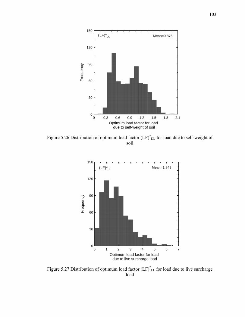
103
0 0.3 0.6 0.9 1.2 1.5 1.8 2.1Optimum load factor for load
due to self-weight of soil
0
30
60
90
120
150
Freq
uenc
y
Mean=0.876(LF)*DL
Figure 5.26 Distribution of optimum load factor (LF)*DL for load due to self-weight of
soil
0 1 2 3 4 5 6 7Optimum load factor for load
due to live surcharge load
0
30
60
90
120
150
Freq
uenc
y
Mean=1.849(LF)*LL
Figure 5.27 Distribution of optimum load factor (LF)*LL for load due to live surcharge
load
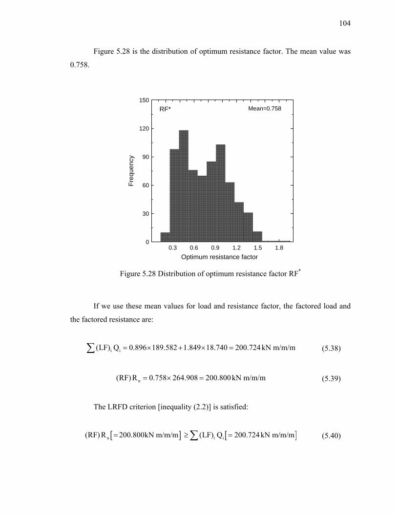
104
Figure 5.28 is the distribution of optimum resistance factor. The mean value was
0.758.
0.3 0.6 0.9 1.2 1.5 1.8Optimum resistance factor
0
30
60
90
120
150
Freq
uenc
y
Mean=0.758RF*
Figure 5.28 Distribution of optimum resistance factor RF*
If we use these mean values for load and resistance factor, the factored load and
the factored resistance are:
i i(LF) Q 0.896 189.582 1.849 18.740 200.724 kN m/m/m= × + × =∑ (5.38)
n(RF) R 0.758 264.908 200.800kN m/m/m= × = (5.39)
The LRFD criterion [inequality (2.2)] is satisfied:
[ ] [ ]n i i(RF) R 200.800kN m/m/m (LF) Q 200.724 kN m/m/m= ≥ =∑ (5.40)

105
5.4.7. Consolidation of calculation results
The values of the optimum factors change from simulation to simulation. These optimum
factors are variable because the representations of soil parameters using Gaussian random
field theory and the location of the corresponding most critical slip surface at the ULS
vary from simulation to simulation. The fluctuations of these optimum factors from
simulation to simulation also results in the fluctuation of RF. This nonuniqueness of ULS
issue can be resolved when we generate a large number of ULSs and calculated the mean
values of optimum factors of these ULSs.
The optimum resistance and load factors and RF values from the six examples are
summarized in Table 5.1. The RF values that are calculated based on Eq. (5.16) and the
AASHTO LF values (LF = 1 for all types of loads) are used. Even for the same target
probability of failure, the RF values in Table 5.1 changes within a wide range.
Table 5.1 Optimum factors from the examples (LF = 1 for all types of loads)
Example q0
(kN/m )Pf LF*DL LF*LL RF* RF
Slope
Example 1 - 0.001 0.907 0.686 0.756
Example 2 - 0.01 0.999 0.779 0.780
Example 3 12 0.001 1.033 1.603 0.809 0.505
Example 4 12 0.01 0.897 1.188 0.752 0.633
Embankment Example 5 12 0.001 0.930 1.088 0.666 0.612
Example 6 12 0.01 0.876 1.849 0.758 0.410
(q0: live surcharge load, Pf: target probability of failure, LF*DL: optimum load factor for
load due to self-weight of soil. LF*LL: optimum load factor for load due to live surcharge
load, RF*: optimum resistance factor, and RF: resistance factor)
Although AASHTO LRFD specifications (2007) suggest that all the load factors
for slope designs are equal to one, it is not reasonable to use those load factors. The use
of LF=1 for all types of loads may be because there has been limited study on load factor
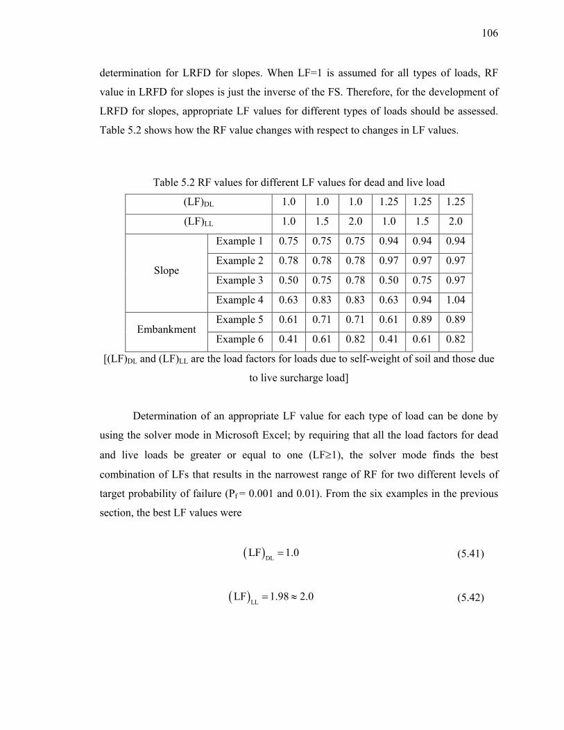
106
determination for LRFD for slopes. When LF=1 is assumed for all types of loads, RF
value in LRFD for slopes is just the inverse of the FS. Therefore, for the development of
LRFD for slopes, appropriate LF values for different types of loads should be assessed.
Table 5.2 shows how the RF value changes with respect to changes in LF values.
Table 5.2 RF values for different LF values for dead and live load
(LF)DL 1.0 1.0 1.0 1.25 1.25 1.25
(LF)LL 1.0 1.5 2.0 1.0 1.5 2.0
Slope
Example 1 0.75 0.75 0.75 0.94 0.94 0.94
Example 2 0.78 0.78 0.78 0.97 0.97 0.97
Example 3 0.50 0.75 0.78 0.50 0.75 0.97
Example 4 0.63 0.83 0.83 0.63 0.94 1.04
Embankment Example 5 0.61 0.71 0.71 0.61 0.89 0.89
Example 6 0.41 0.61 0.82 0.41 0.61 0.82
[(LF)DL and (LF)LL are the load factors for loads due to self-weight of soil and those due
to live surcharge load]
Determination of an appropriate LF value for each type of load can be done by
using the solver mode in Microsoft Excel; by requiring that all the load factors for dead
and live loads be greater or equal to one (LF≥1), the solver mode finds the best
combination of LFs that results in the narrowest range of RF for two different levels of
target probability of failure (Pf = 0.001 and 0.01). From the six examples in the previous
section, the best LF values were
( )DLLF 1.0= (5.41)
( )LLLF 1.98 2.0= ≈ (5.42)

107
Using these LF values, the RF values for the examples are calculated and
summarized in Table 5.3.
Table 5.3 RF values when (LF)DL=1 and (LF)LL=2.0
Example q0
(kN/m ) Pf RF
Slope
Example 1 - 0.001 0.75
Example 2 - 0.01 0.78
Example 3 12 0.001 0.78
Example 4 12 0.01 0.83
Embankment Example 5 12 0.001 0.71
Example 6 12 0.01 0.82
(q0: live surcharge load, Pf: target probability of failure, and RF: resistance factor)
The result in Table 5.3 shows that, when appropriate LFs are determined, the RF
for each target probability of failure varies within a relatively narrow range; the RF value
for target probability of failure equal to 0.001 ranges from 0.71 to 0.78 and that for a
target probability of failure equal to 0.01 varies from 0.78 to 0.83. However, we have
examined the RF values from only 6 examples. To propose appropriate LF values for
each type of loads and RF values for LRFD for slopes, we need to perform extensive
reliability-based slope stability simulations with different conditions in terms of slope
geometry, soil parameters, and external loads.

109
PART III - LRFD OF MSE WALLS
In the early 1960s, Mechanically Stabilized Earth (MSE) walls were devised by Henri
Vidal, a French engineer and architect, and later patented as “Reinforced Earth.” The first
construction of low MSE walls in the United States was in California in 1972. MSE walls
are now the most popular type of retaining structure, and, for transportation applications,
more than half of the retaining structures are MSE walls. The big advantage of an MSE
wall is its economical efficiency. Moreover, MSE wall construction is much easier than
that of other retaining structures.
An MSE wall consists of facing, reinforcement, reinforced soil, retained soil, and
foundation soil (Figure P.1). A backfill material in the “reinforced soil zone” is placed
between layers of horizontal reinforcement. There are several types of reinforcements,
such as steel strips, steel grids, geotextile sheets, and geogrids. However, in this report,
we only consider steel strips as the reinforcement.
Reinforced soil Retained soil
Foundation soil
Facing
Reinforcement
Figure P.1 Cross-sectional view of an MSE wall
MSE walls must satisfy both the external and internal stability criteria. The
external stability criteria include: (1) sliding, (2) overturning, (3) limit bearing capacity

110
failure, and (4) general loss of stability. Internal stability criteria include: (1) structural
failure (rupture) and (2) pullout of the reinforcements. For the LRFD check of the limit
bearing capacity failure of an MSE wall, refer to the literature (Foye, et al. 2006; Foye,
2004; and Scott, 2002).
Each stability criterion (both the external and internal stability criteria) has its
own ULS that may be defined by limit equilibrium analyses. The parameters represented
in Figure P.2 are the variables that are used in defining the ULS equations. For
convenience in notation, the subscripts rf, rt, and fn are used to indicate that the variables
are related to reinforced soil, retained soil, and foundation soil, respectively.
R,rf d,rf d,rf _ max d,rf _ minD ( , , )γ γ γ rt c,rt,γ φ
*fn fn,γ δ
0,rfq
Reinforced soil
Retained soil
Foundation soil
*rfδ
0,rtq
r pK , δ
Figure P.2 Parameters used in ULS equations for MSE walls (DR is the relative density, γd is the dry unit weight, Kr is the coefficient of lateral earth pressure, δp is the interface friction angle between the backfill material in the reinforced soil and the reinforcement, φc is the critical-state friction angle, and δ* is the interface friction angle at the bottom of
the MSE wall)

111
All the variables in Figure P.2 are subject to uncertainties. In this study, the
uncertainties of the parameters δ*rf, φc,rt, δ*
fn, γrf, γrt, γfn, DR,rf, δp, and q0 are assessed.
Using these variables and their uncertainties, a series of reliability analyses are performed,
and RF values for each stability criterion of MSE wall systems proposed based on the
results of these analyses.

112
CHAPTER 6. EXTERNAL STABILITY OF MSE WALLS
6.1. Introduction
This chapter introduces the development of the LRFD method for MSE walls for the two
external stability criteria (sliding and overturning) that are specific to retaining wall
structures. The calculation of RF values for each stability criterion is done in the
following sequence:
1. Identify the ULS equation and the models used in the ULS equation.
2. Identify the component variables that are related to the ULS equation and
models.
3. Select the LFs from the AASHTO LRFD specifications.
4. Evaluate the uncertainties of the component variables and the models
themselves (determine the types of distribution, bias factors, and COVs).
5. Perform reliability analyses until a calculated reliability index is equal to the
target reliability index.
6. Calculate the loads and resistance at the ULS.
7. Calculate the nominal loads and resistance.
8. Compute the optimum RF and LFs.
9. Determine the RF value using the optimum factors.
The assessment of the uncertainties of the soil parameters for MSE walls is quite
different from that for slopes. For the soil parameters for slopes, Gaussian random field
theory was used for the representation of the soil parameters of a statistically
homogeneous soil layer. This is because a statistically homogeneous soil layer of slopes
113
may be extensive, and the mean, bias factor and COV of a specific soil parameter are not
sufficient to capture the effects of the uncertainty in the soil parameter. However, for
MSE walls, the uncertainties of the soil parameters were expressed using their means and
COVs (bias factors, if necessary). This is because the dimensions of an MSE wall are
relatively small, backfill materials for MSE wall construction are quality-controlled not
only by using high quality backfill materials for the reinforced soil and retained soil, but
also by performing proper compaction on them. This means that use of random field
theory would add little value to the analysis.
6.2. Ultimate Limit States Associated with External Stability
A crucial assumption is made in defining the ULS equations for the external stability
ULSs of MSE walls: the reinforced soil mass is assumed to be a solid block, such as a
gravity retaining wall. Ingold (1982) stated that this assumption has worked successfully
in MSE wall designs for external stability criteria. Therefore, the conventional limit
equilibrium analysis for the external stability of a gravity retaining wall can be employed
to define the ULS equations for each of the external stability criteria of an MSE wall
(sliding, overturning, bearing capacity and overall stability criteria).
ULS equations for sliding and overturning criteria are introduced in this section.
The bearing capacity criterion of an MSE wall is similar to that for a shallow foundation.
We could substitute the previous JTRP reports done by Foye and Scott (Foye 2004 and
Scott 2002) for the bearing capacity criterion of MSE walls. In addition, LRFD-based
analysis of overall stability of an MSE wall can be done using the slope stability
guidelines discussed earlier.
6.2.1. Sliding criterion
For MSE wall sliding checks, the live uniform surcharge load acting on the top of the
reinforced soil q0,rf is neglected, while that acting on the top of the retained soil q0,rt is

114
considered (Article 11.5.5 of AASHTO LRFD specifications, 2007). This is because, in
reality, we may have this situation (q0,rt exists while q0,rf does not), which is the worst
case in terms of an external load condition.
A1E
A2EH
L
0,rtq
rfW
rfW tan⋅ δ
Figure 6.1 Forces defining the sliding ULS equation (EA1 and EA2 are the lateral forces due to the active earth pressures caused by the self-weight of the retained soil and the live
uniform surcharge load q0,rt; Wrf is the self-weight of the reinforced soil; H is the MSE wall height; H is the reinforcement length; and δ is the interface friction angle at the
bottom of the MSE wall)
Therefore, the ULS equation for sliding is
A1 A2 rfE + E W tan 0− ⋅ δ = (6.1)
where EA1 and EA2 are the lateral forces due to the active earth pressures caused by the
self-weight of the retained soil and the live uniform surcharge load q0,rt, Wrf is the self-
weight of the reinforced soil, and L is the reinforcement length.

115
EA1+EA2 is the load inducing a sliding of an MSE wall and Wrf tanδ is the
resistance against the sliding. The active earth pressure coefficient KA is used in the
calculation of EA1 and EA2. The active earth pressure coefficient of retained soil is
A1 sinK1 sin
− φ=
+ φ (6.2)
EA1 and EA2 are
2A1 A rt
1E K H2
= γ (6.3)
A2 A 0,rtE K q H= (6.4)
where H is the height of the MSE wall.
In the MSE wall system, generally, an active state occurs when the soil mass is
just about to collapse under a constant vertical stress. The active earth pressure acting on
the reinforced soil develops after some deformation of the retained soil. However, if the
retained soil is in a dense state and is subjected to relatively large strain due to high
overburden pressure and to the wall moment, the mobilized of the retained soil will be
somewhere between the peak and critical-state values. Therefore, the use of peak friction
angle φp to estimate KA, which is recommended in current design guides (AASHTO,
2007 and FHWA, 2001), is questionable because φp is mobilized at small strains and will
drop from φp to the critical-state value φc as sliding develops. Moreover, it is dangerous to
use φp to estimate KA because it will underestimate the lateral forces (EA1 and EA2) acting
on the reinforced soil (KA calculated using φp is less than that calculated using φc). To be
consistent in our design, φc is used to estimate KA using Eq. (6.2). It is known that the φc
in triaxial compression is less than that in plane-strain compression.

116
The self-weight of the reinforced soil is
rf rfW = γ HL (6.5)
In FHWA (2001) and AASHTO (2007) specifications, the interface friction angle
δ at the bottom of an MSE wall is determined as the minimum value between the peak
friction angle of the reinforced soil φp,rf and that of the foundation soil φp,fn:
( )p,rf p,fnmin ,δ = φ φ (6.6)
The minimum value between φp,rf and φp,fn for δ is taken because the sliding of the
reinforced soil can occur either along the foundation soil or the reinforced soil in the
vicinity of the bottom of MSE walls. However, the use of φp in Eq. (6.6) overestimates
the resistance against the sliding of an MSE wall because φp is higher than the actual
interface friction angle at the bottom of MSE walls. Therefore, instead of using φp in Eq.
(6.6) for the δ at the bottom of an MSE wall, it is more reasonable to use δ* which is
defined as
* -1
a
= tan'
⎛ ⎞τδ ⎜ ⎟σ⎝ ⎠
(6.7)
where τ is the shear stress in the horizontal plane and σ′a is the constant vertical stress on
the horizontal plane during sliding. The interface friction angle δ at the bottom of an
MSE wall is:
( )* *rf fnmin ,δ = δ δ (6.8)

117
6.2.2. Overturning criterion
The analysis of the overturning ULS is simpler than that of sliding in terms of defining
the parameters in the ULS equation. Again, the live uniform surcharge load acting on the
top of the reinforced soil is neglected (Article 11.5.5 of AASHTO LRFD specifications,
2007). The ULS equation for overturning is
A1 A2 rfH HE + E W 03 2 2
⎛ ⎞− =⎜ ⎟⎝ ⎠
L (6.9)
The equations for the calculation of EA1, EA2, and Wrf are the same as those used
in the sliding criterion. [Eq. (6.3), Eq. (6.4), and Eq. (6.5)]. In Eq. (6.9), EA1H/3 and
EA2H/2 are the driving moment due to the self-weight of the retained soil and that due to
the live uniform surcharge load q0,rt on the top of an MSE wall, while WrfL/2 is the
resisting moment due to the self-weight of the reinforced soil.
A1E
A2EH
L
0,rtq
rfW
Figure 6.2 Forces defining the overturning ULS equation (EA1 and EA2 are the lateral forces due to the active earth pressures caused by the self-weight of the retained soil and

118
the live uniform surcharge load q0,rt; Wrf is the self-weight of the reinforced soil; H is the MSE wall height; and H is the reinforcement length)
6.3. Determination of LFs for External Stability
The method to determine the LF values from AASHTO LRFD specifications (2007) was
briefly explained in chapter 2. There are two types of loads that induce sliding and
overturning in MSE walls (Figure 6.3): (1) the lateral load EA1 acting on the reinforced
soil due to the self-weight of the retained soil and (2) the lateral load EA2 acting on the
reinforced soil due to the live uniform surcharge load q0,rt on the top of the retained soil.
Since EA1 is induced by a permanent load, the corresponding load factor (the load factor
for active horizontal earth pressure EH given in Table 2.2:) is to be in the 0.9-1.5 range.
EA2 in turn is induced by a live uniform surcharge load; therefore, the load factor of 1.75
given in Table 2.1 should be used. The LF values for the permanent loads are selected
such that, the factored load (LF times permanent load) induces the highest instability on
the wall. In this case, the LF for EA1 is 1.5 because the factored load 1.5EA1 is the highest
possible factored load that will lead to the most instability of an MSE wall against sliding
and overturning.
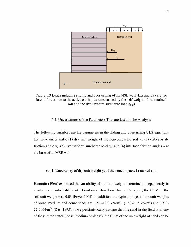
119
A1E
A2E
Reinforced soil Retained soil
Foundation soil
0,rtq
Figure 6.3 Loads inducing sliding and overturning of an MSE wall (EA1 and EA2 are the lateral forces due to the active earth pressures caused by the self-weight of the retained
soil and the live uniform surcharge load q0,rt)
6.4. Uncertainties of the Parameters That are Used in the Analysis
The following variables are the parameters in the sliding and overturning ULS equations
that have uncertainty: (1) dry unit weight of the noncompacted soil γd, (2) critical-state
friction angle φc, (3) live uniform surcharge load q0, and (4) interface friction angles δ at
the base of an MSE wall.
6.4.1. Uncertainty of dry unit weight γd of the noncompacted retained soil
Hammitt (1966) examined the variability of soil unit weight determined independently in
nearly one hundred different laboratories. Based on Hammitt’s report, the COV of the
soil unit weight was 0.03 (Foye, 2004). In addition, the typical ranges of the unit weights
of loose, medium and dense sands are (15.7-18.9 kN/m3), (17.3-20.5 kN/m3) and (18.9-
22.0 kN/m3) (Das, 1995). If we pessimistically assume that the sand in the field is in one
of these three states (loose, medium or dense), the COV of the unit weight of sand can be

120
assessed using the 6σ method, which is explained in Appendix D. Applying the 6σ
method to the three states of sand, a loose sand has the highest COV of 0.03 among them.
Therefore, we will assume, conservatively, that the COV of γd is 0.03.
6.4.2. Uncertainty of critical-state friction angle φc
The critical-state friction angle φc is used to estimate the active earth pressure coefficient
KA; it can be estimated using different apparatuses, such as the triaxial chamber, the
direct shear box or the ring shear apparatus under undrained or drained conditions.
From forty-seven undrained triaxial tests performed on standard Toyoura sand
(D50=0.17mm, emax=0.977, emin=0.597, Gs=2.65) performed by Verdugo and Ishihara
(1996), the mean φc of this sand was 31.7° with a standard deviation of 0.805° resulting
in a COV value equal to 0.025. In addition, ring shear drained tests on Ottawa sand with
different initial relative densities, normal stresses and both dry and wet soil samples, the
maximum COV of φc was reported to be 0.0172 (Negussey et al., 1987). The
corresponding values of COVs are summarized in Table 6.1. The COV of φc in our
analysis is conservatively selected as 0.02, which is slightly higher than the maximum
COV (0.172) in Table 6.1.
Table 6.1 COVs of φc of Ottawa sand from ring shear tests (after Negussey et al., 1987)
Type of sand Sample condition Soil state COV Note
Medium Ottawa Sand
Dry DR=30% 0.0146 9 tests
Saturated DR=30% 0.0172 9 tests
Dry DR varied (30 - 90%) 0.0081 6 tests
Fine Ottawa Sand
Dry Normal stress varied (200 - 1000kPa) 0.0168 9 tests
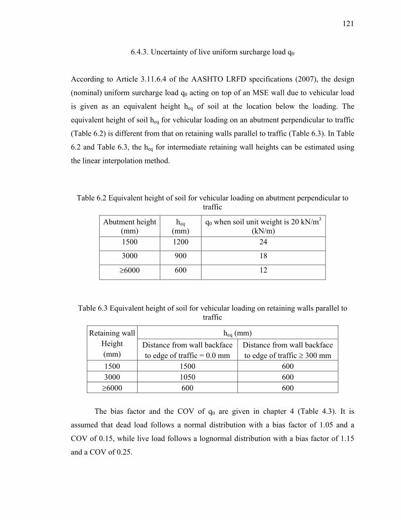
121
6.4.3. Uncertainty of live uniform surcharge load q0
According to Article 3.11.6.4 of the AASHTO LRFD specifications (2007), the design
(nominal) uniform surcharge load q0 acting on top of an MSE wall due to vehicular load
is given as an equivalent height heq of soil at the location below the loading. The
equivalent height of soil heq for vehicular loading on an abutment perpendicular to traffic
(Table 6.2) is different from that on retaining walls parallel to traffic (Table 6.3). In Table
6.2 and Table 6.3, the heq for intermediate retaining wall heights can be estimated using
the linear interpolation method.
Table 6.2 Equivalent height of soil for vehicular loading on abutment perpendicular to traffic
Abutment height (mm)
heq (mm)
q0 when soil unit weight is 20 kN/m3 (kN/m)
1500 1200 24
3000 900 18
≥6000 600 12
Table 6.3 Equivalent height of soil for vehicular loading on retaining walls parallel to traffic
Retaining wall Height (mm)
heq (mm) Distance from wall backface to edge of traffic = 0.0 mm
Distance from wall backface to edge of traffic ≥ 300 mm
1500 1500 600 3000 1050 600
≥6000 600 600
The bias factor and the COV of q0 are given in chapter 4 (Table 4.3). It is
assumed that dead load follows a normal distribution with a bias factor of 1.05 and a
COV of 0.15, while live load follows a lognormal distribution with a bias factor of 1.15
and a COV of 0.25.

122
When a variable (x) has a lognormal probability distribution, its natural logarithm
(ln(x)) is normally distributed. The probability density function of a lognormal
distribution is
2
21 1 ln xp(x) exp
2x 2
⎡ ⎤⎛ ⎞− λ⎢ ⎥= − ⎜ ⎟⎜ ⎟⎢ ⎥σ π ζ⎝ ⎠⎣ ⎦ (6.10)
where λ and ζ are the mean and standard deviation of the lognormal distribution, ln(x).
The mean μ and standard deviation σ of x are
2
exp2
ζμ λ⎡ ⎤
= +⎢ ⎥⎣ ⎦
(6.11)
( ) ( )( )2 2exp 2 exp 1= + −σ λ ζ ζ (6.12)
Thus, ζ and λ can be modified as
2
ln 1 σζμ
⎡ ⎤⎛ ⎞= +⎢ ⎥⎜ ⎟
⎝ ⎠⎢ ⎥⎣ ⎦ (6.13)
( ) 21ln2
λ μ ζ= − (6.14)
To define a lognormal distribution, these two parameters (ζ and λ) are necessary.
These values are needed when we perform reliability analysis using a Microsoft Excel
spreadsheet to calculate the equivalent mean and standard deviation of lognormal
distributed data. For example, when the nominal live uniform surcharge load q0 is 12
123
kN/m and the bias factor and COV are 1.15 and 0.25, respectively, the mean μ and
standard deviation σ of q0 are
bias factor nominal value 1.15 12 13.8 kN/m= × = × =μ (6.15)
0.25 13.8 3.45 kN/m= × = × =COVσ μ (6.16)
Thus, the standard deviation ζ and mean λ of ln(x) are
2 23.45ln 1 ln 1 0.24613.8
⎡ ⎤ ⎡ ⎤⎛ ⎞ ⎛ ⎞= + = + =⎢ ⎥ ⎢ ⎥⎜ ⎟⎜ ⎟⎝ ⎠⎝ ⎠⎢ ⎥ ⎢ ⎥⎣ ⎦⎣ ⎦
σζμ
(6.17)
( ) ( )2 21 1ln ln 13.8 0.246 2.5942 2
= − = − =λ μ ζ (6.18)
6.4.4. Uncertainty of interface friction angle δ (δ*) at the base of an MSE wall
Pradhan et al. (1988) conducted experiments to estimate the interface friction angles δ of
hollow cylindrical specimens with different initial void ratios and confining stresses
using a torsional shear apparatus. A Plane Strain (PS) condition prevails in the case of an
MSE wall undergoing sliding failure. Using the Torsional Simple Shear (TSS) apparatus,
an element inside a specimen can be sheared under PS conditions with constant vertical
stress, as shown in Figure 6.4. The TSS apparatus does not allow radial displacement of
the sample and automatically controls the vertical stress σa, which remains constant
during shearing. Thus, the results from the TSS tests can be used to emulate closely the
condition prevailing in the field (the vertical force acting at the bottom of an MSE wall
due to the self-weight of reinforced soil does not change but total lateral force increases
to have sliding of an MSE wall) for the sliding case of an MSE wall and to estimate an
interface friction angle when sliding failure occurs.

124
Pradhan et al. (1988) performed TSS tests on one-dimensionally consolidated
Toyoura sand under different “constant” vertical stresses σa (29.4-196.2 kN/m2). The
relationship between the stress ratio τ/σa (the ratio of the shear stress τ to the constant
vertical stress σa on the horizontal plane) and the shear strain γ for the dense specimens
showed that τ/σa increases to reach a peak value at a small shear strain and then
approximates the critical-state value (τ/σa)r (=tanδ*r). For the loose samples, τ/σa
monotonically increases to reach the critical-state stress ratio (τ/σa)r. The critical-state
stress ratio (τ/σa)r is independent of the initial void ratio and confining stress. During
simple shearing, the angle α1 of the maximum principal stress direction to the vertical
plane changed within a very small strain (γ less than 1%) and remained constant in the
range of 45°−50° to the critical-state state. Later on, α1 will be denoted as the major
principal stress direction angle.
a'σ
τ
aF
T
ip 0p
r'σ
t'σ
t 0ε =r 0ε =
1α
1σ
i 0 r 0 ap p K= = σ = σPradhan & Tatsuoka (1988)Torsional simple shear apparatus
Figure 6.4 Torsional shearing under constant vertical stress σ′a on the horizontal plane using the TSS apparatus (σ′a: vertical effective stress; σ′t: effective stress in torsional direction; σ′r: effective stress in radial direction; α1: major principal stress direction
angle; and K0: coefficient of lateral earth pressure at rest )

125
For the purpose of developing the relationship between the friction angle φ and
the corresponding interface friction angle δ, we compared φ to the corresponding δ based
on data from the literature (Pradhan et al., 1988). Figure 6.5 represents the peak friction
angle φp and the maximum interface friction angle δ*p during shearing when the vertical
stress σa is 98kN/m2. Figure 6.6 shows the same for different vertical stresses (σa = 98-
196.2kN/m2). A purely contractive specimen (initial void ratio e = 0.893 when σc =
5kN/m2) will not show a peak behavior during shearing and in that case φp is equal to φc.
Similarly, the maximum stress ratio (τ/σa)max for this specimen will be equal to the
critical-state stress ratio (tanδ*r). Therefore, from Figure 6.5 and Figure 6.6, we can
approximate the values of φc and δ*r for Toyoura sand to be 35° and 30°.
c 35φ = o
r 30δ = o
0.6 0.7 0.8 0.9Initial void ratio at σ'c=5kN/m2
25
30
35
40
45
50
Pea
k fri
ctio
n an
gle
φ p a
nd
max
imum
inte
rface
fric
tion
angl
e δ p
( τ m
ax/σ
a ) φp: Peak friction angle
δp: Max. interface friction angle
e=0.893
TSS resultσ'a=98kN/m2
07.0878 ep 32.9088 1175.7144 e− ×φ = + ×
2R 0.9943=
05.4763 ep 27.2639 382.4589 e− ×δ = + ×2R 0.9887=
Figure 6.5 Estimation of φc and δr from the relationship between φp and δp with different initial void ratio when σa = 98kN/m2 (φp and δp of a purely contractive specimen are equal
to φc and δr, respectively)

126
c 35φ = o
r 30δ = o
0.6 0.7 0.8 0.9Initial void ratio at σ'c=5kN/m2
25
30
35
40
45
50
Pea
k fri
ctio
n an
gle
φ p a
nd
max
imum
inte
rface
fric
tion
angl
e δ p
( τ m
ax/σ
a )
φp δp
φp δp
φp
e=0.893
TSS resultα=45°∼50°
δp
φp δp
σ'a=49.1kN/m2
σ'a=29.4kN/m2
σ'a=98.1kN/m2
σ'a=196.2kN/m2
Figure 6.6 Estimation of φc and δr from the relationship between φp and δp with different initial void ratio for different vertical stresses (σa = 98-196.2kN/m2) on the horizontal plane (φp and δp of a purely contractive specimen are equal to φc and δr, respectively)
The peak interface friction angle δ*p may or may not be mobilized along the
bottom of an MSE wall at sliding failure. In other words, it is unlikely that δ*p is
mobilized and sustained for every point along the sliding surface at the moment of sliding.
For sliding of MSE walls, large horizontal movements of the reinforced soil mass must
occur; therefore, δ* may be expected to be closer to δ*r. In addition, it is safer to use δ*
r in
design.
The relationship between φc and δ*r can be explained using the Mohr circle
diagram for stress given in Figure 6.7. The Mohr circle is drawn for the stresses at the
critical state. Given that the angle that the maximum principal stress direction makes with
the vertical direction is equal to α1, from the Mohr circle, the critical-state shear stress τr
and the vertical stress σa on the sliding plane can be expressed as:
( )1r 1 32
1
tan1 tan
ατ = σ − σ
+ α (6.19)

127
( )21 1 3r
a 1 21 1
tantan 1 tan
α σ + στσ = σ − =
α + α (6.20)
where σ1 and σ3 are the major and minor principal stresses.
Then, the stress ratio σ1/σ3 can be expressed in terms of φc as:
c1
3 c
1 sin1 sin
+ φσ=
σ − φ (6.21)
aσ
rτ
*rδ
cφ
σ
τ
1σ3σ1α
pole
Figure 6.7 Relationship between critical-state friction angle φc and critical-state interface friction angle δ*
r explained using the Mohr circle diagram (τr and σa are the critical-state shear stress and the vertical stress on the sliding plane; σ1 and σ3 are the major and minor
principal stresses; and α1 is the major principal stress direction angle)
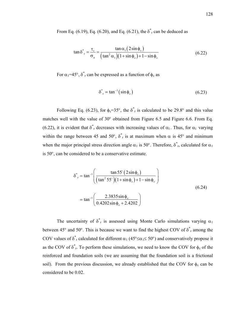
128
From Eq. (6.19), Eq. (6.20), and Eq. (6.21), the δ*r can be deduced as
( )( )( )
1 c* rr 2
a 1 c c
tan 2sintan
tan 1 sin 1 sinα φτ
δ = =σ α + φ + − φ
(6.22)
For α1=45°, δ*r can be expressed as a function of φc as
( )* 1r ctan sin−δ = φ (6.23)
Following Eq. (6.23), for φc=35°, the δ*r is calculated to be 29.8° and this value
matches well with the value of 30° obtained from Figure 6.5 and Figure 6.6. From Eq.
(6.22), it is evident that δ*r decreases with increasing values of α1. Thus, for α1 varying
within the range between 45 and 50°, δ*r is at maximum when α is 45° and minimum
when the major principal stress direction angle α1 is 50°. Therefore, δ*r, calculated for α1
is 50°, can be considered to be a conservative estimate.
( )( )( )
c* 1r 2
c c
1 c
c
tan 55 2sintan
tan 55 1 sin 1 sin
2.3835sintan0.4202sin 2.4202
−
−
⎛ ⎞φ⎜ ⎟δ =⎜ ⎟+ φ + − φ⎝ ⎠
⎛ ⎞φ= ⎜ ⎟φ +⎝ ⎠
o
o
(6.24)
The uncertainty of δ*r is assessed using Monte Carlo simulations varying α1
between 45° and 50°. This is because we want to find the highest COV of δ*r among the
COV values of δ*r calculated for different α1 (45°≤α1≤ 50°) and conservatively propose it
as the COV of δ*r. To perform these simulations, we need to know the COV for φc of the
reinforced and foundation soils (we are assuming that the foundation soil is a frictional
soil). From the previous discussion, we already established that the COV for φc can be
considered to be 0.02.

129
Figure 6.8 shows the distribution of δ*r resulting from the simulation with
normally distributed φc and the mean equal to 30° having a COV of 0.02. From the
simulations, the bias factors and COVs of the δ*r are given in Table 6.4 for the cases of
α1=45° and α1=50°. The highest COV was 0.0156 for α1=45°. Conservatively, the COV
for the δ*r is selected as 0.02.
Figure 6.8 Distribution of the critical-state interface friction angle δ*r when φc=30° using
Monte Carlo simulations
Table 6.4 Bias factor and COV of the critical-state interface friction angle δ*r (α1 is the
major principal stress direction angle)
??1 φc (°)
δ*r
(°) Standard
deviation (°)COV Bias factor
45°
30 26.6 0.414 0.0156 1.000 32 27.9 0.424 0.0152 1.000 34 29.2 0.430 0.0147 1.000 36 30.4 0.434 0.0142 1.000
50°
30 24.4 0.360 0.0147 1.000 32 25.5 0.365 0.0143 1.000 34 26.7 0.369 0.0138 1.000 36 27.7 0.371 0.0134 1.000
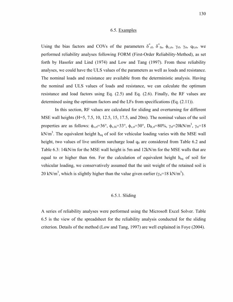
130
6.5. Examples
Using the bias factors and COVs of the parameters δ*rf, δ*
fn, φc,rt, γrf, γrt, q0,rt, we
performed reliability analyses following FORM (First-Order Reliability-Method), as set
forth by Hasofer and Lind (1974) and Low and Tang (1997). From these reliability
analyses, we could have the ULS values of the parameters as well as loads and resistance.
The nominal loads and resistance are available from the deterministic analysis. Having
the nominal and ULS values of loads and resistance, we can calculate the optimum
resistance and load factors using Eq. (2.5) and Eq. (2.6). Finally, the RF values are
determined using the optimum factors and the LFs from specifications (Eq. (2.11)).
In this section, RF values are calculated for sliding and overturning for different
MSE wall heights (H=5, 7.5, 10, 12.5, 15, 17.5, and 20m). The nominal values of the soil
properties are as follows: φc,rf=36°, φc,fn=33°, φc,rt=30°, DR,rf=80%, γrf=20kN/m3, γrt=18
kN/m3. The equivalent height heq of soil for vehicular loading varies with the MSE wall
height, two values of live uniform surcharge load q0 are considered from Table 6.2 and
Table 6.3: 14kN/m for the MSE wall height is 5m and 12kN/m for the MSE walls that are
equal to or higher than 6m. For the calculation of equivalent height heq of soil for
vehicular loading, we conservatively assumed that the unit weight of the retained soil is
20 kN/m3, which is slightly higher than the value given earlier (γrt=18 kN/m3).
6.5.1. Sliding
A series of reliability analyses were performed using the Microsoft Excel Solver. Table
6.5 is the view of the spreadsheet for the reliability analysis conducted for the sliding
criterion. Details of the method (Low and Tang, 1997) are well explained in Foye (2004).
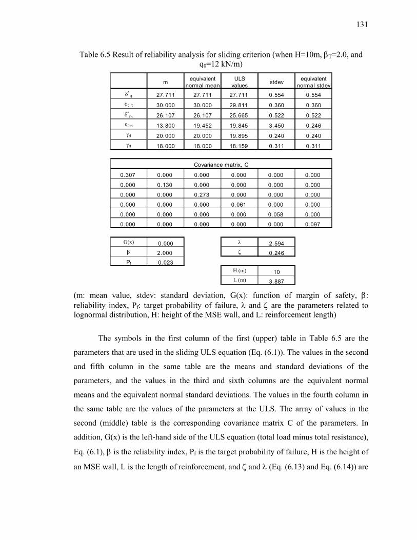
131
Table 6.5 Result of reliability analysis for sliding criterion (when H=10m, βT=2.0, and q0=12 kN/m)
m equivalentnormal mean
ULSvalues stdev equivalent
normal stdevδ∗
rf 27.711 27.711 27.711 0.554 0.554φc,rt 30.000 30.000 29.811 0.360 0.360δ∗
fn 26.107 26.107 25.665 0.522 0.522q0,rt 13.800 19.452 19.845 3.450 0.246γrf 20.000 20.000 19.895 0.240 0.240γrt 18.000 18.000 18.159 0.311 0.311
0.307 0.000 0.000 0.000 0.000 0.000
0.000 0.130 0.000 0.000 0.000 0.000
0.000 0.000 0.273 0.000 0.000 0.000
0.000 0.000 0.000 0.061 0.000 0.000
0.000 0.000 0.000 0.000 0.058 0.000
0.000 0.000 0.000 0.000 0.000 0.097
G(x) 0.000 λ 2.594β 2.000 ζ 0.246Pf 0.023
H (m) 10L (m) 3.887
Covariance matrix, C
(m: mean value, stdev: standard deviation, G(x): function of margin of safety, β: reliability index, Pf: target probability of failure, λ and ζ are the parameters related to lognormal distribution, H: height of the MSE wall, and L: reinforcement length)
The symbols in the first column of the first (upper) table in Table 6.5 are the
parameters that are used in the sliding ULS equation (Eq. (6.1)). The values in the second
and fifth column in the same table are the means and standard deviations of the
parameters, and the values in the third and sixth columns are the equivalent normal
means and the equivalent normal standard deviations. The values in the fourth column in
the same table are the values of the parameters at the ULS. The array of values in the
second (middle) table is the corresponding covariance matrix C of the parameters. In
addition, G(x) is the left-hand side of the ULS equation (total load minus total resistance),
Eq. (6.1), β is the reliability index, Pf is the target probability of failure, H is the height of
an MSE wall, L is the length of reinforcement, and ζ and λ (Eq. (6.13) and Eq. (6.14)) are

132
the parameters that define the lognormal distribution of the live uniform surcharge load
on the top of an MSE wall.
The lateral force EA1 due to active action of the self-weight of the retained soil
and the lateral force EA2 due to active action by the live uniform surcharge load as well as
the total resistance at the ULS are shown in Table 6.6. In Table 6.7, the FS and the
nominal values of the EA1, EA2, and resistance against sliding are calculated using the
nominal values of the soil parameters. Finally, the RF value is computed using the
AASHTO LFs, the ULS values of loads and resistance (Table 6.6), and the nominal
values of loads and resistance (Table 6.7).
Table 6.6 ULS values of loads and resistance for sliding
EA1 313.329 kN/m Dead load (EA1) 313.329 kN/mEA2 64.032 kN/m Live load (EA2) 64.032 kN/mWrf 784.089 kN/m Total resistance (Wrftanδ) 377.361 kN/m
tanδ 0.481
Table 6.7 Nominal values of loads and resistance and FS for sliding
EA1 300.000 kN/m Dead load (EA1) 300.000 kN/mEA2 40.000 kN/m Live load (EA2) 40.000 kN/mWrf 787.900 kN/m Total resistance (Wrftanδ) 386.103 kN/m
tanδ 0.490 FS= 1.136
Table 6.8 Calculation of optimum factors and RF using AASHTO LFs for sliding
(LF)DL* = 1.04 (LF)DL= 1.5 0.70(LF)LL* = 1.60 (LF)LL= 1.75 0.91
RF* = 0.98 1.07
(LF)DL* / (LF)DL=(LF)LL* / (LF)LL=
RF= [(LF)DL
* and (LF)LL* are the optimum load factors for dead and live load, RF* is the
optimum resistance factor, (LF)DL and (LF)LL are the AASHTO load factors, and RF is the resistance factor]
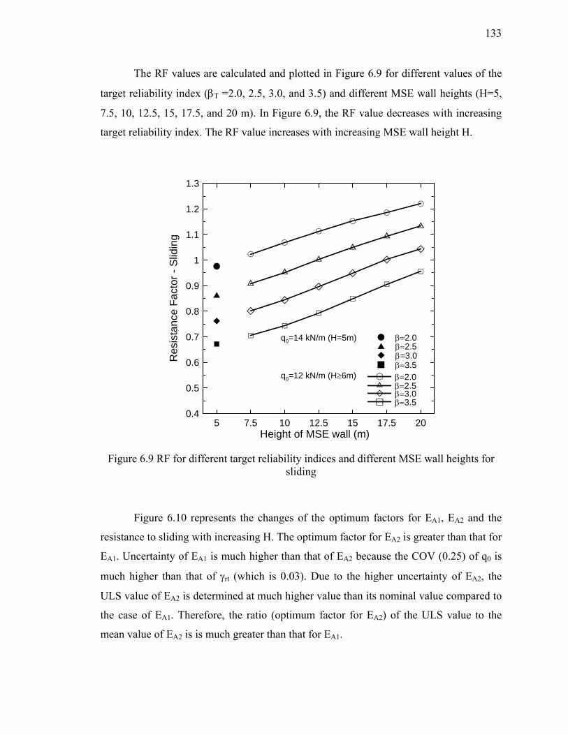
133
The RF values are calculated and plotted in Figure 6.9 for different values of the
target reliability index (βT =2.0, 2.5, 3.0, and 3.5) and different MSE wall heights (H=5,
7.5, 10, 12.5, 15, 17.5, and 20 m). In Figure 6.9, the RF value decreases with increasing
target reliability index. The RF value increases with increasing MSE wall height H.
5 7.5 10 12.5 15 17.5 20Height of MSE wall (m)
0.4
0.5
0.6
0.7
0.8
0.9
1
1.1
1.2
1.3R
esis
tanc
e Fa
ctor
- S
lidin
g
β=2.0 β=2.5 β=3.0
β=2.0β=2.5β=3.0
q0=12 kN/m (H≥6m)
q0=14 kN/m (H=5m)
β=3.5
β=3.5
Figure 6.9 RF for different target reliability indices and different MSE wall heights for sliding
Figure 6.10 represents the changes of the optimum factors for EA1, EA2 and the
resistance to sliding with increasing H. The optimum factor for EA2 is greater than that for
EA1. Uncertainty of EA1 is much higher than that of EA2 because the COV (0.25) of q0 is
much higher than that of γrt (which is 0.03). Due to the higher uncertainty of EA2, the
ULS value of EA2 is determined at much higher value than its nominal value compared to
the case of EA1. Therefore, the ratio (optimum factor for EA2) of the ULS value to the
mean value of EA2 is is much greater than that for EA1.
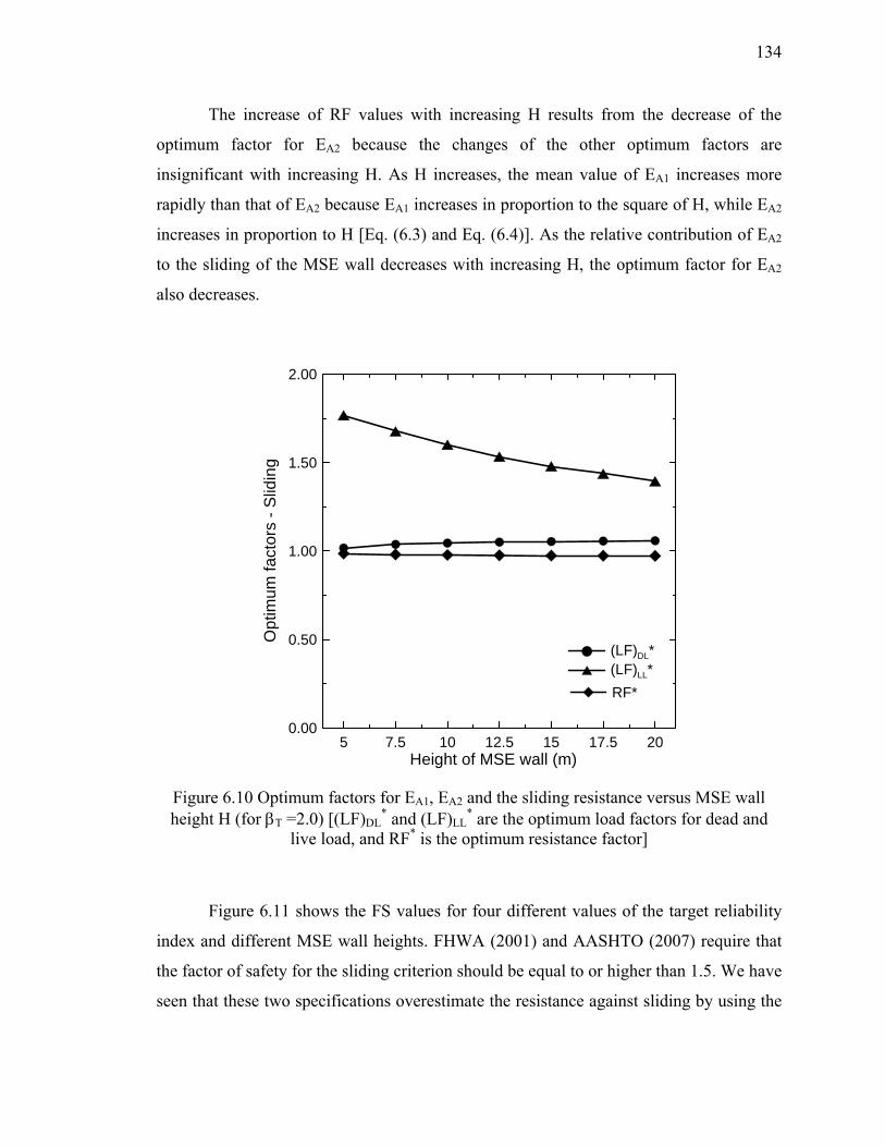
134
The increase of RF values with increasing H results from the decrease of the
optimum factor for EA2 because the changes of the other optimum factors are
insignificant with increasing H. As H increases, the mean value of EA1 increases more
rapidly than that of EA2 because EA1 increases in proportion to the square of H, while EA2
increases in proportion to H [Eq. (6.3) and Eq. (6.4)]. As the relative contribution of EA2
to the sliding of the MSE wall decreases with increasing H, the optimum factor for EA2
also decreases.
5 7.5 10 12.5 15 17.5 20Height of MSE wall (m)
0.00
0.50
1.00
1.50
2.00
Opt
imum
fact
ors
- Slid
ing
(LF)DL*(LF)LL*RF*
Figure 6.10 Optimum factors for EA1, EA2 and the sliding resistance versus MSE wall height H (for βT =2.0) [(LF)DL
* and (LF)LL* are the optimum load factors for dead and
live load, and RF* is the optimum resistance factor]
Figure 6.11 shows the FS values for four different values of the target reliability
index and different MSE wall heights. FHWA (2001) and AASHTO (2007) require that
the factor of safety for the sliding criterion should be equal to or higher than 1.5. We have
seen that these two specifications overestimate the resistance against sliding by using the

135
peak friction angle φp instead of using δ* (Eq. (6.7)) for the interface friction angle δ, and
underestimate the active force by using φp in calculating the active earth pressure
coefficient KA (Eq. (6.2)) instead of using φc. For this reason, the minimum required FS
value of 1.5 in the specifications must be revised to a lower value in our design. Thus, the
FS values in Figure 6.11 are not directly comparable to the 1.5 minimum.
5 7.5 10 12.5 15 17.5 20Height of MSE wall (m)
1
1.1
1.2
1.3
1.4
1.5
1.6
Fact
or o
f Saf
ety
- Slid
ing
β=2.0 β=2.5 β=3.0
β=2.0β=2.5β=3.0
q0=12 kN/m (H≥6m)
q0=14 kN/m (H=5m)
β=3.5
β=3.5
Figure 6.11 FS as a function of target reliability index and MSE wall height for sliding
6.5.2. Overturning
The same procedure that was used for sliding was applied to the calculation of the RF
values for overturning. Table 6.9 shows the Microsoft Excel spreadsheet used to perform
the reliability analysis. For the 10m-high MSE wall, the reinforcement length is
determined to be 3.38 m, satisfying the target reliability index βT of 2.0 when the mean
values and standard deviations of the parameters are the values shown in Table 6.9.

136
Table 6.9 Result of reliability analysis for overturning criterion (when the height of MSE wall H=10m, target reliability index βT=2.0 and nominal q0=12 kN/m)
mean equivalentnormal mean
ULSvalues stdev equivalent
normal stdevφ2 30.000 30.000 29.847 0.360 0.360 0.130 0.000 0.000 0.000
q0,rt 13.800 20.833 21.297 3.450 0.246 0.000 0.061 0.000 0.000
γrf 20.000 20.000 19.915 0.240 0.240 0.000 0.000 0.058 0.000
γrt 18.000 18.000 18.116 0.311 0.311 0.000 0.000 0.000 0.097
G(x) 0.000 H (m) 10 λ 2.594
β 2.000 L (m) 3.709 ζ 0.246
Pf 0.023
Covariance matrix, C
(m: mean value, stdev: standard deviation, G(x): function of margin of safety, β: reliability index, Pf: target probability of failure, λ and ζ are the parameters related to lognormal distribution, H: height of the MSE wall, and L: reinforcement length)
The values in the fourth column in Table 6.9 are the values of the parameters at
the ULS. The driving and resisting moments at the ULS are calculated using these values.
In Table 6.10, the sum of the driving moments due to EA1 (lateral load from the self-
weight of retained soil) and EA2 (lateral load from the live uniform surcharge load) is
equal to the resisting moment against overturning (1012.679 kN/m + 357.143 kN/m =
1369.822 kN/m), as the definition of the ULS.
Table 6.10 Driving and resisting moments at the overturning ULS
Driving moment due to the dead load (EA1H/3) 1012.679 kN/mDriving moment due to the live load (EA2H/2) 357.143 kN/mResistance moment against overturning (WrfL/2) 1369.822 kN/m
The values of the nominal driving and resisting moments are given in Table 6.11.
These moments were calculated using the nominal values of the parameters. The factor of
safety for this particular case was 1.15.

137
Table 6.11 Nominal driving and resisting moments and FS for overturning
Driving moment due to the dead load (EA1H/3) 1000.000 kN/mDriving moment due to the live load (EA2H/2) 200.000 kN/mResistance moment against overturning (WrfL/2) 1375.668 kN/m
FS= 1.15
Table 6.12 Calculation of optimum factors and RF using AASHTO LFs for overturning
(LF)DL* = 1.01 (LF)DL= 1.50 0.68(LF)LL* = 1.79 (LF)LL= 1.75 1.02
RF* = 0.996 0.98
(LF)LL* / (LF)LL=
RF=
(LF)DL* / (LF)DL=
[(LF)DL
* and (LF)LL* are the optimum load factors for dead and live load, RF* is the
optimum resistance factor, (LF)DL and (LF)LL are the AASHTO load factors, and RF is the resistance factor]
The RF values for different target reliability indices and different MSE wall
heights are shown in Figure 6.12. Similarly to sliding, the RF value increases with
decreasing target reliability index and increasing MSE wall height. However, the increase
of RF value for overturning is less significant than that for sliding.

138
5 7.5 10 12.5 15 17.5 20Height of MSE wall (m)
0.4
0.5
0.6
0.7
0.8
0.9
1
1.1
1.2
Res
ista
nce
Fact
or -
Ove
rturn
ing
β=2.0 β=2.5 β=3.0
β=2.0β=2.5β=3.0
q0=12 kN/m (H≥6m)
q0=14 kN/m (H=5m)
β=3.5
β=3.5
Figure 6.12 RF for different target reliability indices and different MSE wall heights for overturning
Figure 6.13 shows the changes of the optimum factors for EA1, EA2 and the
overturning resistance with increasing MSE wall height H. The trend of the changes in
these optimum factors for overturning is similar to those for sliding. Similarly to sliding,
the reason for the RF increase with increasing H is the significant decrease of the
optimum factor (LF)LL* for EA2 with an increasing H. The increase of (LF)LL
* with
increasing H can be explained as follows: As H increases, the relative contribution of EA2,
to total loading decreases compared to that of EA1 to total loading; therefore, (LF)LL* also
decreases.

139
5 7.5 10 12.5 15 17.5 20Height of MSE wall (m)
0.00
0.50
1.00
1.50
2.00
Opt
imum
fact
ors
- Ove
rturn
ing
(LF)DL*(LF)LL*RF*
Figure 6.13 Optimum factors for EA1, EA2 and the overturning resistance versus MSE wall height (for βT =2.0) [(LF)DL
* and (LF)LL* are the optimum load factors for dead and
live load, and RF* is the optimum resistance factor]
Figure 6.14 illustrates the FS values for different target reliability indices and
different H. The highest FS was about 1.43. From the FHWA (2001) and AASHTO
(2007) specifications, it is required that a factor of safety for overturning criterion should
be equal to or higher than 2.0. In section 6.5.1, we found that these two specifications
underestimate the active force acting on the reinforced soil because of the use of φp in
calculating KA (Eq. (6.2)). The minimum required FS value in these two specifications
(FS=2.0) would be less if KA were calculated using φc.

140
5 7.5 10 12.5 15 17.5 20Height of MSE wall (m)
1
1.1
1.2
1.3
1.4
1.5
1.6
Fact
or o
f Saf
ety
- Ove
rturn
ing
β=2.0 β=2.5 β=3.0
β=2.0β=2.5β=3.0
q0=12 kN/m (H≥6m)
q0=14 kN/m (H=5m)
β=3.5
β=3.5
Figure 6.14 FS as a function of target reliability index and MSE wall height for overturning

141
CHAPTER 7. INTERNAL STABILITY OF MSE WALLS
7.1. Introduction
This chapter addresses the LRFD checks for internal stability of MSE walls (pullout and
structural failure of the steel-strip reinforcement). The framework and procedure for the
RF value calculation for internal stability are the same as those for external stability.
7.2. Internal Stability Ultimate Limit States
ULS equations are developed using limit equilibrium analysis for the two internal
stability limit states of an MSE wall (pullout and structural failure of the steel-strip
reinforcement). At the ULSs of these two internal stability criteria, the load Tmax is the
maximum tensile force on the steel-strip reinforcement. To calculate Tmax for one
particular steel-strip reinforcement, the overburden pressure is multiplied by the
coefficient of lateral earth pressure Kr and the tributary area of the reinforcement. The
tributary area is defined as an influence area for each steel-strip reinforcement that is
equal to the horizontal spacing sh times the vertical spacing sv of the reinforcement. The
assessment of the uncertainty of Tmax is the most difficult step in our analysis, not only
because of limited data but also because of the very high level of uncertainty in the
coefficient of lateral earth pressure Kr. The current design specifications (FHWA, 2001
and AASHTO, 2007) use a simplified method to compute Kr. In our design method, the
existing “Coherent gravity method” is modified so that we can predict Kr with less
uncertainty compared to the simplified method.

142
7.2.1. Pullout of steel-strip reinforcement
The steel-strip reinforcement pullout ULS takes place when the maximum tensile force
Tmax acting on the reinforcement reaches the pullout resistance of the reinforcement. Tmax
is described as the maximum lateral force acting on the backfill soil over the tributary
area of the reinforcement. Therefore, Tmax at a depth z from the top of an MSE wall is
( )max h v h r v v h r rf 0,rf v hT = σ' s s K σ' s s K z q s s= = γ + (7.1)
where σ′h is the horizontal effective stress; sv and sh are the vertical and horizontal
spacing of the steel-strip reinforcement, respectively; Kr is the coefficient of lateral earth
pressure; and σ′v is the vertical effective stress.
Pullout resistance of the steel-strip reinforcement is defined as the frictional
resisting force against the maximum tensile force acting on the reinforcement:
PO R v eR = 2C ' L bσ (7.2)
where CR is the pullout resistance factor that is comparable to the coefficient of friction,
Le is the effective length of the reinforcement, and b is the width of the steel-strip
reinforcement.
The live uniform surcharge q0,rf acting on the top of reinforced soil is neglected in
the pullout resistance RPO calculation (Eq. (7.2)) according to the AASHTO and FHWA
specifications. According to these two specifications, vehicular loads and other live loads
are excluded in the pullout resistance calculations (FHWA, 2001, section 4.3 and
AASHTO, 2007, section 11.5.5). However, q0,rf is considered when we estimate Tmax.
The reason for neglecting q0,rf in the pullout resistance calculation and considering q0,rf in
assessing Tmax may be because of the concern that q0,rf may not be distributed evenly
along the reinforcement or q0,rf may not contribute to full mobilization of the pullout

143
resistance. Either way, we retain that design provision here. Pullout resistance of the
steel-strip reinforcement is modified as
( )PO R rf eR = 2C z L bγ (7.3)
Since we are comparing Tmax acting on the steel-strip reinforcement to the
maximum resisting force against the pullout of the reinforcement, the pullout ULS
equation at a reinforcement level equal to z from the top of the MSE wall can be written
as:
( ) ( )r rf 0,rf v h R rf eK z q s s 2C z L b=0γ + − γ (7.4)
7.2.2. Structural failure of steel-strip reinforcement
The steel-strip structural failure ULS occurs when the maximum tensile force acting on a
steel-strip reinforcement reaches the yield force of the reinforcement. The tensile force Ty
at yield of a steel-strip reinforcement is
y y cT = f A (7.5)
where fy is the yield strength of the steel-strip reinforcement, and Ac is the cross-sectional
area of the steel-strip reinforcement.
The maximum tensile force acting on a steel-strip reinforcement was defined in
the previous section (Eq. (7.1)). Therefore, the steel-strip structural failure ULS at a depth
z from the top of the MSE wall is
( ) ( )r rf 0,rf v h y cK z q s s f A =0γ + − (7.6)

144
7.3. Determination of LFs for Internal Stability Calculations
The maximum tensile force Tmax acting on a steel-strip reinforcement can be divided into
two loads, as shown in Figure 7.1: (1) the lateral load Fr,DL acting on the reinforcement
due to the self-weight of the reinforced soil and (2) the lateral force Fr,LL due to the live
uniform surcharge load on the top of the reinforced soil. Tmax can be written as
( )max r rf 0,rf v h r rf v h r 0,rf v h r,DL r,LLT = K z q s s K z s s K q s s F Fγ + = γ + = + (7.7)
Similarly to the cases of sliding and overturning, the LF for Fr,LL is 1.75 because
Fr,LL is induced by a live uniform surcharge load on the top of the MSE wall (Figure 7.1).
Determination of the LF for Fr,DL is more complicated. The condition near the top of the
reinforced soil is more likely to be an at-rest state; while the condition for greater depths
approaches an active condition. From Table 2.4, the ranges of LF for lateral earth
pressure at rest condition and active condition are 0.90-1.35 and 0.90-1.50, respectively.
LF is determined in a way that the factored load will induce the most instability against
the structural failure and pullout of the reinforcement of the MSE wall. Therefore, for
conservativeness, we are using the maximum LF of active earth pressure (1.5) as the LF
for Fr,DL because the load factored by the maximum load factor will destabilize the
internal stabilities of MSE walls.

145
0,rfq
r,LLFr,DLF
0,rtq
Reinforced soil Retained soil
Foundation soil
Figure 7.1 Loads for pullout and structural failure of the steel-strip reinforcement (Fr,DL and Fr,LL are the lateral loads acting on the reinforcement due to the self-weight of the
reinforced soil and due to the live uniform surcharge load on the top of the reinforced soil q0,rf)
7.4. Uncertainty of Locus of Maximum Tensile Force along the Steel-Strip
Reinforcements
The potential failure zone inside the reinforced soil that separates the active zone and the
stationary zone is assumed to coincide with the locus of the maximum tensile forces Tmax
at each reinforcement level, as shown in Figure 7.2. The reinforcement length inside the
active zone is indicated as La and that inside the stationary zone is named the effective
length and indicated as Le. Therefore, the total length of the reinforcement is the sum of
La and Le. The AASHTO (2007) and FHWA (2001) design specifications for MSE walls
specify that the minimum required length of reinforcement (L) is 70% of the height H of
an MSE wall. Also, FHWA (2001) prescribes that the minimum effective length of
reinforcement Le is 1m. Only the pullout resistance along the effective length of the
reinforcement is considered and used as the total resistance against pullout of the
reinforcements. To calculate the total length of the required reinforcement length L, the

146
uncertainty of the reinforcement length La embedded in the active wedge should be
assessed.
H
L
Active zone
Resisting zone
L
T Tmax
La Le
La: Length embedded in the active wedge
La: Effective lengthof the reinforcement
L
T Tmax
Retained soil
Foundation soil
Figure 7.2 Location of maximum tensile forces on the reinforcements and distribution of tensile force along the reinforcements
Juran (1977) found from laboratory studies that the failure surface resembled a
logarithmic spiral. In addition, Corte (1977) confirmed that the locus of the maximum
tensile forces is a logarithmic spiral using finite element analysis (Figure 7.2). The design
specifications (AASHTO, 2007 and FHWA, 2001) approximate the failure zone as
bilinear. Therefore, La, the distance from the facing of the MSE wall, can be expressed
as:

147
( )( )
a
H0.3H, 0 z 2L z =
H0.6 H-z , z H2
⎧ ≤ ≤⎪⎪⎨⎪ ≤ ≤⎪⎩
(7.8)
where z is the depth from the top of the MSE wall.
Schlosser et al. (1978) presented the measurements of the location of the
maximum tensile force Tmax from five completed MSE walls. The uncertainty of the
locus of the maximum tensile force was assessed using the data in his literature. Out of
five completed MSE walls, the measurements of the maximum tensile forces of one MSE
wall were excluded because the values of those measurements were very low. Four
measurements of the maximum tensile forces near the base of MSE walls were also
excluded while assessing the uncertainty of the locus of the maximum tensile force
because, even though the difference between the measured and the corresponding
predicted La are small, the high ratios of the measured to the corresponding predicted La
induce higher bias factors. Finally, twenty-four measurements were used in assessing the
uncertainty of the maximum tensile force, and the bias factor and COV turned out to be
0.825 and 0.16, respectively. The location of the measurements is normalized by the
height of MSE wall H and shown in Figure 7.3. L′a (dashed-doted line in Figure 7.3) is
the length of reinforcement inside the active wedge obtained from a regression analysis
by fitting the measurements of the locations of Tmax to a bilinear equation.

148
0 0.2 0.4 0.6 0.8 1x/H
0
0.2
0.4
0.6
0.8
1
y/H
ASAHIGAOKA
GRIGNY
LILLE
THIONVILLE
La from specifications
L'a: La fitted with measurement
La,CAM: La by CAM
Figure 7.3 Location of the maximum tensile force normalized by the height of MSE walls
Except the two points near the base of the MSE walls, the locations of La defined
by Eq. (7.8) can be considered as the upper boundary of the measured data. Therefore,
conservatively, we could use the location of La defined by Eq. (7.8) in design of MSE
walls.
7.5. Uncertainties of the Parameters That are Used in the Analysis of the Internal
Stability of MSE Walls
The uncertainties of several parameters that are used in the ULS equations for pullout and
structural failure of the steel-strip reinforcement were already assessed in the previous
chapter. The following variables are the additional parameters which uncertainties that
have to be assessed to perform reliability analyses for internal stability of MSE walls: (1)
dry unit weight of the compacted soil, (2) maximum dry unit weight and minimum dry
unit weight for frictional soils, (3) relative density of backfill soil in the reinforced soil,

149
(4) coefficient of lateral earth pressure Kr, (5) pullout resistance factor CR of steel-strip
reinforcement, and (6) yield strength of steel-strip reinforcement.
7.5.1. Uncertainty of dry unit weight of the compacted soil
The backfill material in the reinforced soil of MSE walls requires a highly frictional
material that has durability, good drainage, and a low Plasticity Index (PI less than 6). To
prevent corrosion of reinforcements, the backfill material in the reinforced soil should not
contain organic matter or detrimental materials (AASHTO, 2007 and FHWA, 2001).
Therefore, well-graded frictional soil is used to build the MSE wall because it has higher
strength and thus maximizes the friction between the soil and the steel-strip
reinforcements. AASHTO standard T-27 imposes constraints on limits the particle size
distribution of backfill soils of MSE walls, as shown in Table 7.1. The backfill soil of an
MSE wall is an A-1 soil according to the AASHTO classification system (ASTM D3282;
AASHTO M145) and GP-GM (poorly graded gravel - silty gravel) according to the
Unified classification system (ASTM D2487).
Table 7.1 Particle size distribution for backfill soils of MSE walls (AASHTO T-27)
Sieve size (mm) Percent passing (%)Diameter or
Sieve number
102 100 4 in.
0.425 0-60 Sieve No. 40
0.075 0-15 Sieve No. 200
Backfill soils in the reinforced soil zone are compacted to more than 95% relative
compaction. A nuclear device is typically used to control the degree of compaction of the
fills. From 230 field tests on a dam construction site (Mt. Cenis Dam in France), the COV
of the dry unit weight of the compacted silty-sandy gravel soil was found to be 0.012

150
(Lacroix and Horn, 1973). The truck-mounted French AGS probe nuclear device was
used to measure the unit weights. From these results, we assume that the COV of dry unit
weight of the compacted backfill material for the reinforced zone is similar to the COV
value (0.012) that Lacroix and Horn (1973) observed.
Since silty-sandy gravel is typically classified as GP-GM in the Unified
Classification System, it is acceptable to use this value (0.012) as the COV of the
compacted backfill soil because the soil used in dam construction is comparable. The
uncertainty of the dry unit weight of the compacted granular soil (COV=0.012) is less
than that of the natural soil (COV=0.03, see section 6.4.1) because controlled compaction
results in less variability of the void ratio of the soil.
7.5.2. Uncertainty of maximum dry unit weight and minimum dry unit weight for
frictional soils
Muszynski (2006) performed tests following the ASTM standards (ASTM D 4253
and ASTM D4254) to evaluate γdmax and γdmin of three different types of sand (Manistee
Dune sand, Traverse City Fill sand, and Concrete sand). For each type of sand, two tests
were performed. Table 7.2 shows the COVs for γdmax of those three sands that are
assessed using Nσ method. The Nσ method is explained in detail in Appendix D.
Table 7.2 γdmax measured using ASTM D4253
Type of sand Mean (kN/m3)
Difference in γdmax between two measurements (%) COV Note
Manistee Dune Sand 17.22 0.017 0.0009
COV estimated using Nσ method
Traverse City Fill Sand 17.51 0.172 0.0087
Concrete Sand 18.93 0.019 0.0009

151
Six tests were conducted for each sand to find γdmin following the ASTM D4254
standard. The means and the corresponding standard deviations of γdmin for these three
sands are provided in Table 7.3. To propose general guidelines that are conservative, we
take the COVs of γdmax and γdmin to be 0.0087 and 0.0024, the highest of the values for the
three sands.
Table 7.3 γdmin measured using ASTM D4254
Type of sand Mean (kN/m3)
Standard deviation (kN/m3) COV Note
Manistee Dune Sand 14.69 0.021 0.0015 6 tests for each type of sand
Traverse City Fill Sand 15.33 0.038 0.0024
Concrete Sand 15.68 0.033 0.0021
7.5.3. Uncertainty of relative density of backfill soil in the reinforced soil
As mentioned earlier, the backfill soil is to be compacted to 95% relative compaction.
Poulos and Hed (1973) demonstrated that there is an approximately linear correlation
between the relative density DR and relative compaction (Figure 7.4). The data points
used in Figure 7.4 are obtained from different types of soils varying from very uniform,
medium sand to coarse sand. The relative density DR of the backfill soil corresponding to
95% or higher relative compaction ranges approximately from 70% to 100%, as indicated
by the shaded region in Figure 7.4.

152
85 90 95 100Relative compaction (%)
0
20
40
60
80
100
Rel
ativ
e de
nsity
(%)
85 90 95 100Relative compaction (%)
0
20
40
60
80
100
Rel
ativ
e de
nsity
(%)
Figure 7.4 Relationship between relative density and relative compaction
DR is expressed in terms of unit weight as follows:
d max d d minR
d dmax dmin
D γ γ − γ= ×
γ γ − γ (7.9)
The uncertainty involved in the dry unit weight γd, the maximum dry unit weight
γdmax, and the minimum dry unit weight γdmin can be used to assess the uncertainty of
relative density. Monte Carlo simulations using Eq. (7.9) were performed to estimate the
means and standard deviations of DR. In the simulation, γdmax, γdmin, and γd of the
compacted backfill soil in the reinforced soil can be considered as independent variables.
According to the previous sections (sections 7.5.1 and 7.5.2), the COVs of γdmax
and γdmin are 0.0087 and 0.0024, and that of γd of the compacted backfill material in the
reinforced soil is 0.012. Since we do not know γdmax and γdmin in the field, we consider
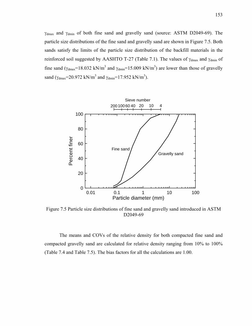
153
γdmax and γdmin of both fine sand and gravelly sand (source: ASTM D2049-69). The
particle size distributions of the fine sand and gravelly sand are shown in Figure 7.5. Both
sands satisfy the limits of the particle size distribution of the backfill materials in the
reinforced soil suggested by AASHTO T-27 (Table 7.1). The values of γdmax and γdmin of
fine sand (γdmax=18.032 kN/m3 and γdmin=15.009 kN/m3) are lower than those of gravelly
sand (γdmax=20.972 kN/m3 and γdmin=17.952 kN/m3).
0.01 0.1 1 10 100Particle diameter (mm)
0
20
40
60
80
100
Per
cent
fine
r
Fine sandGravelly sand
200 10060 40 20 10 4Sieve number
Figure 7.5 Particle size distributions of fine sand and gravelly sand introduced in ASTM D2049-69
The means and COVs of the relative density for both compacted fine sand and
compacted gravelly sand are calculated for relative density ranging from 10% to 100%
(Table 7.4 and Table 7.5). The bias factors for all the calculations are 1.00.

154
Table 7.4 COVs of relative density of compacted fine sand
DRγd
(kN/m3)mean(DR)
Stdev(DR) COV
100% 18.032 100% 7.41% 0.07490% 17.676 90% 7.25% 0.08180% 17.334 80% 7.14% 0.08970% 17.005 70% 7.06% 0.10160% 16.688 60% 7.00% 0.11750% 16.382 50% 6.97% 0.13940% 16.088 40% 6.98% 0.17530% 15.804 30% 7.01% 0.23420% 15.530 20% 7.11% 0.35610% 15.265 10% 7.18% 0.718
Table 7.5 COVs of relative density of compacted gravelly sand
DRγd
(kN/m3)mean(DR)
Stdev(DR) COV
100% 20.972 100% 8.89% 0.08990% 20.625 90% 8.70% 0.09780% 20.289 80% 8.51% 0.10670% 19.965 70% 8.40% 0.12060% 19.650 60% 8.30% 0.13850% 19.345 50% 8.24% 0.16540% 19.049 40% 8.22% 0.20630% 18.763 30% 8.25% 0.27520% 18.485 20% 8.31% 0.41610% 18.215 10% 8.42% 0.842
For a given relative density, the COV of compacted gravelly sand is higher than
that of compacted fine sand. Conservatively, we are proposing the COV values (Table
7.5) of compacted gravelly sand with a relative density ranging from 70% to 100% as the
uncertainty of relative density of the backfill soil in the reinforced zone.
155
7.5.4. Uncertainty of coefficient of lateral earth pressure Kr
Much care is required in estimating the coefficient of lateral earth pressure Kr because it
has the highest uncertainty from all the parameters used in the ULSs of internal stability
of MSE walls.
7.5.4.1. The conventional methods of Kr estimation
Allen, T. et al. (2001) introduced four methods to estimate Kr: (1) coherent gravity
method; (2) tieback wedge method; (3) FHWA structure stiffness method; and (4)
simplified method. The FHWA structure stiffness method was used to estimate Kr in the
previous version of the MSE wall design and construction guidelines (FHWA-RD-89-
043); the so-called simplified method has been used in a more recent version of the
guidelines (FHWA-SA-96-071 & FHWA-NHI-00-043). Among those four methods, the
simplified method works best for MSE walls with steel-strip reinforcement because the
method has the least uncertainty. However, we found that the modification of the existing
“coherent gravity method” enables Kr prediction with less uncertainty compared to that of
the “simplified method” reported by Allen et al. (2001).
7.5.4.2. Modified coherent gravity method
The original “coherent gravity method” was developed from the work done by Juran and
Schlosser (1978), Schlosser (1978), and Schlosser and Segrestin (1979) to estimate Kr in
precast panel-faced MSE wall systems (Allen et al., 2001).
The coherent gravity method assumes that Kr varies linearly from K0 at the top of
an MSE wall to KA at a depth zcr = 6m from the top of an MSE wall and Kr remains
constant for depths greater than 6m (Figure 7.6). The depth zcr will be allowed to vary
later in this chapter.
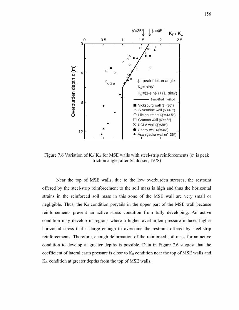
156
12
8
4
0
Ove
rbur
den
dept
h z
(m)
Vicksburg wall (φ'=36°)
0 0.5 1 1.5 2 2.5Kr / KA
Silvermine wall (φ'=40°)Lile abutment (φ'=43.5°)Granton wall (φ'=46°)UCLA wall (φ'=38°)Griony wall (φ'=36°)Asahigaoka wall (φ'=36°)
Simplified method
φ'=35° φ'=46°
K0 = sinφ'φ': peak friction angle
KA =(1-sinφ') / (1+sinφ')
Figure 7.6 Variation of Kr/ KA for MSE walls with steel-strip reinforcements (φ′ is peak friction angle; after Schlosser, 1978)
Near the top of MSE walls, due to the low overburden stresses, the restraint
offered by the steel-strip reinforcement to the soil mass is high and thus the horizontal
strains in the reinforced soil mass in this zone of the MSE wall are very small or
negligible. Thus, the K0 condition prevails in the upper part of the MSE wall because
reinforcements prevent an active stress condition from fully developing. An active
condition may develop in regions where a higher overburden pressure induces higher
horizontal stress that is large enough to overcome the restraint offered by steel-strip
reinforcements. Therefore, enough deformation of the reinforced soil mass for an active
condition to develop at greater depths is possible. Data in Figure 7.6 suggest that the
coefficient of lateral earth pressure is close to K0 condition near the top of MSE walls and
KA condition at greater depths from the top of MSE walls.

157
The original coherent gravity method assumes that an active condition has
developed at depths greater than 6m from the top of the MSE walls. Regression analysis
using the available field measurement data for Tmax was conducted as part of the present
study to ascertain the depth below which an active condition would prevail. This will be
explained later in detail.
7.5.4.2.1. K0 estimation
The original coherent gravity method uses the following equation to estimate K0
(proposed by Jaky, 1944):
0K 1 sin= − φ (7.10)
The method uses φp to estimate K0 using Eq. (7.10). K0 estimation using Eq.
(7.10) involves a large uncertainty as the measured data points are widely scattered with
respect to the values calculated using the equation. In addition, Eq. (7.10) does not work
well for high friction angles (φp>40°) because the estimated K0 value is then very low.
Fang et al. (1997) back-calculated the coefficients of lateral earth pressure at rest
for normally consolidated granular soil (K0nc) from the measurement of the lateral earth
pressure acting against a rigid wall and concluded that K0nc varies from 0.4 to 0.48. Air-
pluviated Ottawa sand was used to construct the backfill (Gs=2.65, emax=0.76, emin=0.50,
D60=0.36mm, D10=0.23mm). Hendron (1963) evaluated a relationship between K0 and
initial void ratio e0. He concluded that K0 of Minnesota sand varied from 0.33 to 0.48 and
that K0 increases as the initial void ratio increases, as shown in Figure 7.7.

158
0.4 0.5 0.6 0.7 0.8Initial void ratio e0
0.3
0.35
0.4
0.45
0.5
Coe
ffici
ent K
0nc o
f ear
th p
ress
ure
at re
st
Figure 7.7 Relationship between K0 and e0 of Minnesota sand
In addition, Okochi and Tatsuoka (1984) performed a series of K0-consolidation
tests on reconstituted Toyoura sand using a Double-cell K0-triaxial apparatus and found
that K0nc varied from 0.34 to 0.49. From the results of the tests, K0 not only depended on
the sample preparation method but also on the initial void ratio. Even though K0 values
for the samples prepared using the wet-tamped method is slightly lower than those for the
samples prepared using the air-pluviated method, the trend shows that the coefficient of
lateral earth pressure at rest increases with increasing initial void ratio e0.
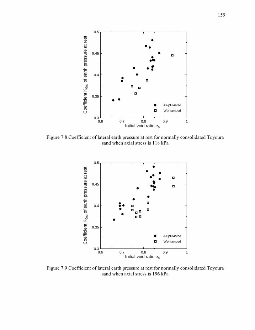
159
0.6 0.7 0.8 0.9 1Initial void ratio e0
0.3
0.35
0.4
0.45
0.5
Coe
ffici
ent K
0nc o
f ear
th p
ress
ure
at re
st
Air-pluviated
Wet-tamped
Figure 7.8 Coefficient of lateral earth pressure at rest for normally consolidated Toyoura sand when axial stress is 118 kPa
0.6 0.7 0.8 0.9 1Initial void ratio e0
0.3
0.35
0.4
0.45
0.5
Coe
ffici
ent K
0nc o
f ear
th p
ress
ure
at re
st
Air-pluviated
Wet-tamped
Figure 7.9 Coefficient of lateral earth pressure at rest for normally consolidated Toyoura sand when axial stress is 196 kPa

160
From the aforementioned work, we expect high relative densities (70-100%) for
the compacted backfill soil in the reinforced soil, and, therefore, it is acceptable to
assume that the upper and lower bounds of K0 for dense sand are 0.35 and 0.45.
Therefore, we can use 0.4 for the expected value of K0 for the backfill soil in the
reinforced soil.
Researchers (e.g. Broms and Ingelson, 1971; Sherif et al., 1984; Carder et al.,
1977) reported that compacted sand has a higher K0 value when the following two
conditions are met: (1) the sand is compacted under a higher overburden stress, as higher
confinement prevents the rebound of soil and (2) the sand is densified under a laterally
constrained condition (as in the case of soil behind a rigid retaining wall). However, the
reinforced soil near the top of an MSE wall is compacted under relatively low overburden
stresses and does not have significant lateral constraints. Therefore, we cannot expect a
significant increase in K0 due to compaction of the reinforced soil of an MSE wall.
Moreover, the measured field data for the maximum tensile forces prove that there is not
a significant effect of compaction on K0 for MSE walls.
7.5.4.2.2. KA estimation
The critical-state friction angle φc is used in Eq. (6.2) to estimate the coefficient KA of
active earth pressure. The reason for using φc to estimate KA was explained earlier. In
general, the values of φc of backfill material for the reinforced soil are not reported in the
literature. Therefore, a range of φc values (30°-36°) is considered. By comparing the field
measurements for the Tmax of the steel-strip reinforcements reported in Allen et al. (2001)
with the corresponding predicted Tmax values varying φc (30°-36°), regression analysis is
conducted by fixing zcr = 6m to find the best value of φc which will induce the least
uncertainty in predicting Kr. From the results of regression analysis, the best value φc in
this respect was found to be 33°, resulting in a value of KA equal to 0.295.
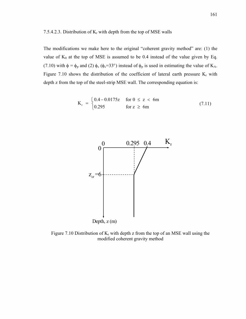
161
7.5.4.2.3. Distribution of Kr with depth from the top of MSE walls
The modifications we make here to the original “coherent gravity method” are: (1) the
value of K0 at the top of MSE is assumed to be 0.4 instead of the value given by Eq.
(7.10) with φ = φp and (2) φc (φc=33°) instead of φp is used in estimating the value of KA.
Figure 7.10 shows the distribution of the coefficient of lateral earth pressure Kr with
depth z from the top of the steel-strip MSE wall. The corresponding equation is:
r
0.4 0.0175z for 0 z 6mK
0.295 for z 6m− ≤ <⎧
= ⎨ ≥⎩ (7.11)
0 0.295 0.4
crz =6
Depth, z (m)
rK0
Figure 7.10 Distribution of Kr with depth z from the top of an MSE wall using the modified coherent gravity method
162
7.5.4.2.4. Bias factor and COV of Kr following the modified coherent gravity method
In the full-scale field tests, the maximum strain is measured along the steel-strip
reinforcement. After that, the maximum tensile force acting on the steel-strip
reinforcement Tmax is calculated by multiplying the corresponding strains by the elastic
modulus of deformation Er of the reinforcement. This method works well because the
steel-strip reinforcement can be considered as an elastic material within the small strain
range.
Figure 7.11 shows the relationship between the measured and predicted maximum
tensile force Tmax,pred. values acting on steel-strip reinforcements. The measured and
predicted Tmax are located in the x and y axis, respectively. The prediction of the Tmax was
calculated using Eq. (7.11). The data for the measured maximum tensile force Tmax,meas.
were collected from 76 measurements obtained from full-scale tests on thirteen MSE
walls reinforced using steel-strip reinforcements. Two measurements of Tmax near the
bottom of an MSE wall were eliminated in this analysis because, even though the
difference between the measured values and the corresponding predicted values are
small, the high ratios of the measured data to the corresponding predicted values result in
higher bias factors. Figure 7.11 shows that Eq. (7.1) overestimates Tmax in the steel-strip
reinforcement because most of the points are on the left side of the dashed line
(Tmax,pred.=Tmax,meas.).

163
0 20 40 60 80 100Measured maximum tensile force Tmax,meas. (kN/m)
0
20
40
60
80
100
Pre
dict
ed m
axim
um te
nsile
forc
e T m
ax,p
red. (k
N/m
)
Line for Tmax,pred=Tmax,meas.
Regression line
Figure 7.11 Relationship between the measured and predicted maximum tensile forces based on the modified coherent gravity method
The ratio of the measured to the predicted maximum tensile force
Tmax,meas./Tmax,pred. is plotted with respect to depth z from the top of the MSE wall (Figure
7.12). There is no discernible depth bias to the data but the variability of the prediction
seems greater at shallower depths (we will ignore that in our analysis). The bias factor for
the prediction of the maximum tensile force at each reinforcement level is 0.666 and the
COV is 0.347. Therefore, the expected value of the Tmax acting on the steel-strip
reinforcement is about two thirds of Kr calculated from Eq. (7.11).

164
16
12
8
4
0
Dep
th fr
om th
e to
p of
MS
E w
all (
m)
0 0.2 0.4 0.6 0.8 1 1.2 1.4Ratio of the measured Tmax to the prediced Tmax
0.666
Figure 7.12 Ratio of measured to predicted Tmax with depth from the top of MSE walls (average value=0.666)
( )r,with bias correction
0.666 0.4 0.0175z 0.266 0.012z for 0 z 6mK
0.666 0.295 0.196 for z 6m× − = − ≤ <⎧⎪= ⎨× = ≥⎪⎩
(7.12)
The values of the maximum tensile forces predicted using Eq. (7.12) are
compared with the measured values in Figure 7.13. The figure shows that the estimation
of Tmax is better when the bias factor of 0.666 is applied to the values predicted using Eq.
(7.11). Figure 7.14 illustrates that the residuals in the predictions with bias correction
follow an almost normal distribution. This agreement provides some assurance that we
can be concluded that the present study can successfully predict the coefficient of lateral
earth pressure Kr with Eq. (7.12).

165
0 20 40 60 80 100Measured maximum tensile force Tmax (kN/m)
0
20
40
60
80
100
Pre
dict
ed m
axim
um te
nsile
forc
e m
ultip
lied
by b
ias
fact
or 0
.666
×Tm
ax (k
N/m
)
Figure 7.13 Relationship between predicted Tmax multiplied by bias factor and measured Tmax based on the modified coherent gravity method
16
12
8
4
0
Dep
th fr
om th
e to
p of
MS
E w
all (
m)
-1 -0.5 0 0.5 1Residual of Kr prediction
Figure 7.14 Residuals of Kr estimation with depth from the top of MSE walls
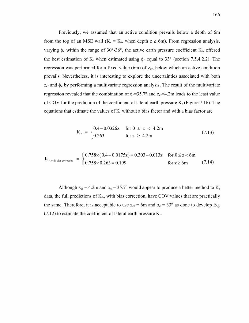
166
Previously, we assumed that an active condition prevails below a depth of 6m
from the top of an MSE wall (Kr = KA when depth z ≥ 6m). From regression analysis,
varying φc within the range of 30°-36°, the active earth pressure coefficient KA offered
the best estimation of Kr when estimated using φc equal to 33° (section 7.5.4.2.2). The
regression was performed for a fixed value (6m) of zcr, below which an active condition
prevails. Nevertheless, it is interesting to explore the uncertainties associated with both
zcr and φc by performing a multivariate regression analysis. The result of the multivariate
regression revealed that the combination of φc=35.7° and zcr=4.2m leads to the least value
of COV for the prediction of the coefficient of lateral earth pressure Kr (Figure 7.16). The
equations that estimate the values of Kr without a bias factor and with a bias factor are
r
0.4 0.0326z for 0 z 4.2mK
0.263 for z 4.2m− ≤ <⎧
= ⎨ ≥⎩ (7.13)
( )r,with bias correction
0.758 0.4 0.0175z 0.303 0.013z for 0 z 6mK
0.758 0.263 0.199 for z 6m× − = − ≤ <⎧⎪= ⎨× = ≥⎪⎩
(7.14)
Although zcr = 4.2m and φc = 35.7° would appear to produce a better method to Kr
data, the full predictions of KA, with bias correction, have COV values that are practically
the same. Therefore, it is acceptable to use zcr = 6m and φc = 33° as done to develop Eq.
(7.12) to estimate the coefficient of lateral earth pressure Kr.

167
16
14
12
10
8
6
4
2
0
Dep
th fr
om th
e to
p of
MS
E w
all (
m)
Back-calculated Kr from measurement in the fields
0 0.2 0.4 0.6Lateral earth pressure coefficient Kr
Kr estimated using Eq.(40)(with bias correction)
Kr estimated using Eq.(39)(without bias correction)
Bias factor=0.666COV=0.347
Depth zcr= 6mKa = 0.295(φc=33°)
Figure 7.15 Result of the regression analysis of Kr on z with zcr = 6m and φc = 33°
16
14
12
10
8
6
4
2
0
Dep
th fr
om th
e to
p of
MS
E w
all (
m)
Back-calculated Kr from measurement in the fields
0 0.2 0.4 0.6Lateral earth pressure coefficient Kr
Kr estimated using Eq.(42)(with bias correction)
Kr estimated using Eq.(41)(without bias correction)
Bias factor=0.758COV=0.343
Depth zcr= 4.2mKa = 0.263 (φc=35.7°)
Kr estimated using Eq.(40)(with bias correction)
Figure 7.16 Result of the regression analysis of Kr on zcr = 4.2m, φc = 35.7° and z
168
7.5.5. Uncertainty of pullout resistance factor CR
There are three popular methods to assess the coefficient of friction CR: (1) direct shear
test between the reinforcement material and the soil, (2) pullout test using specially
designed equipment in the laboratory, and (3) pullout test from a full-scale MSE wall or
scaled model.
The CR suggested by AASHTO (2007) and FHWA (2001) is:
p
R
p
tan -1.8min z +1.8, 2.0 for 0 z < 6m
6C =tan for z 6m
⎧ ⎡ φ ⎤⎛ ⎞≤⎪ ⎢ ⎥⎜ ⎟
⎨ ⎝ ⎠⎣ ⎦⎪ φ ≥⎩
(7.15)
The solid line in Figure 7.17 represents the CR predicted by Eq. (7.15) assuming
that φp is 32°. The data points in Figure 7.17 are CR values from pullout tests for steel-
strip reinforcements installed in backfill materials ranging from silty sands to coarse
gravels. The CR value predicted by Eq. (7.15) is very conservative because Eq. (7.15) was
chosen so as to be close to the lower bound for the pullout test data shown in Figure 7.17.
So there is a high bias factor in CR calculated using Eq. (7.15).

169
0 2 4 6 8 108
6
4
2
0
Dep
th fr
om th
e to
p of
MSE
wal
l (m
)
0 2 4 6 8 10Pullout resistance factor, CR
CR proposed by FHWA
Possible range of CRUsing Eq.(111)
Figure 7.17 Comparison between CR suggested by AASHTO and FHWA specifications and CR data point from pullout tests (Data points from Commentary of the 1994
AASHTO Standard Specifications for Highway Bridges)
In our study, we developed a different approach for estimating CR. Many
researchers have studied the interface friction angle between steels and soils. The
interface friction angle was examined with different levels of roughness of steel,
confining stress, and relative density. Since the steel-strip reinforcement provided by the
Reinforced Earth Company is ribbed, it is acceptable to conclude the reinforcement is
relatively rough. Using the data from the literature written by Lings and Dietz (2005), the
interface friction angle was estimated considering the effect of the relative density and
confining stress (the data are given in Appendix E). The direct shear apparatus with a
sample that has the reinforcing material (steel) on one side below or above the shear
plane and soil on the other side was used to measure the interface friction angles. The
best equation for the prediction of the interface friction angle is
170
'= 13.1 1.59 ln 1.15100
⎧ ⎫⎡ ⎤⎛ ⎞⎛ ⎞⎪ ⎪⋅ − ⋅ + +⎢ ⎥⎜ ⎟⎨ ⎬⎜ ⎟⎜ ⎟⎢ ⎥⎝ ⎠⎝ ⎠⎪ ⎪⎣ ⎦⎩ ⎭
vRp cv
A
DP
σδ δ (7.16)
where pA is the reference pressure, which is 100kPa, and δcv is the critical-state interface
friction angle.
The bias factor and the COV of the model (Eq. (7.16)) were 1.00 and 0.07,
respectively. Thus, the pullout resistance factor CR is
tan=R pC δ (7.17)
The possible range for the mean value of CR calculated using Eq. (7.17) varying
the parameters in Eq. (7.16) within the following ranges: (1) DR,rf = 70-100%, (2) γd,rf =
17-20kN/m3, and (3) δcv = 25-32° is drawn with dashed lines in Figure 7.17. The
measured data points of CR are widely scattered. Our predictions of the expected values
of CR fall within the scattered data.
7.5.6. Uncertainty of yield strength of steel-strip reinforcement
The uncertainty of the yield strength of the steel-strip reinforcement was assessed using
90 test results provided by the Reinforced Earth Company. Steel-strip reinforcements
were made of Grade 65 steel, and from ASTM A-572, Grade 65 steel should have a yield
strength higher than 450 MPa. Out of 90 data points, the minimum and maximum yield
strength were 453 MPa and 584 MPa, and the average was 491 MPa, as shown in Figure
7.18.

171
0
5
10
15
20
25
30
440 460 480 500 520 540 560 580 600
Yield stress (MPa)
Freq
uenc
y
Figure 7.18 Distribution of yield strength of steel-strip reinforcements (data acquired from the Reinforced Earth Company)
Assuming that the nominal yield strength of the steel-strip reinforcement is 450
MPa, the bias factor was 1.09 and the COV was 0.05.
yf = 450 MPa (7.18)
7.6. Examples
A series of reliability analyses using First-Order Reliability Method (FORM) were
performed accounting for the bias factors and COVs of the parameters γrf, q0,rf, fy, DR,rf,
δcv, Kr, and δp related to the ULS equations for pullout and structural failure of steel-strip
reinforcement.
The ULS equation (Eq. (7.4)) for the steel-strip pullout basically compares the
maximum tensile force acting on the reinforcement Tmax with the maximum pullout
resistance RPO. For a given target reliability index, the RF value is calculated by finding
the effective length of the reinforcement that produces the target reliability index.
Similarly to the pullout case, the ULS equation (Eq. (7.6)) for the steel-strip structural

172
failure compares Tmax to the yield force Ty of the reinforcement. The RF value is obtained
by searching for the reinforcement depth that produces the given target reliability index.
Seven different MSE wall heights (H=5, 7.5, 10, 12.5, 15, 17.5, 20 m) and four
different target reliability indices (βT =2.0, 2.5, 3.0, and 3.5) were considered. The two
nominal live uniform surcharge loads q0 are used depending on MSE wall height: (1)
14kN/m for 5m-high MSE walls and (2) 12 kN/m for MSE walls more than 6m-tall. In
addition, we assume that the pavement has a thickness of 0.3m.
Within the maximum ranges of horizontal and vertical spacing (FHWA, 2001),
the combinations of two different horizontal spacings sh (sh=0.375 and 0.75m) and three
different vertical spacings sv (sv=0.3, 0.6, and 0.8m) of steel-strip reinforcement are
considered for pullout of the reinforcement, while the combinations of two different
horizontal spacings (sh=0.75 and 0.375m) and six different vertical spacings (sv=0.3, 0.4,
0.5, 0.6, 0.7 and 0.8m) are considered for structural failure of steel-strip reinforcement.
7.6.1. Pullout of steel-strip reinforcement
The same procedure used for external stability criteria is applied to the RF value
computation for the steel-strip reinforcement pullout. The means of the parameters are
the values given in the second column in Table 7.6. The table represents the results of the
reliability analysis conducted for the following case: sv=0.6m, sh=0.75m, H=20m, βT=3.0,
the nominal q0=12kN/m, and the reinforcement depth z=0.60m. The effective length Le
for βT=3.0 is calculated to be 6.87m.

173
Table 7.6 Result of reliability analysis for pullout of steel-strip reinforcement (when sv=0.6m, sh=0.75m, z=0.60m, H=20m, βT=3.0, and the nominal q0=12 kN/m)
meq
uiva
lent
norm
al m
ean
ULS
valu
esst
dev
equi
vale
ntno
rmal
std
evK
r0.
259
0.25
90.
452
0.09
0.09
00.
008
0.00
00.
000
0.00
00.
000
0.00
0D
R80
8074
.612
9.60
9.60
00.
000
92.1
600.
000
0.00
00.
000
0.00
0γ r
f20
2019
.982
0.24
0.24
00.
000
0.00
00.
058
0.00
00.
000
0.00
0q 0
,rf13
.819
.735
20.1
433.
450.
246
0.00
00.
000
0.00
00.
061
0.00
00.
000
δ cv
28.5
28.5
28.2
830.
780.
782
0.00
00.
000
0.00
00.
000
0.61
20.
000
η δp
11
0.92
10.
070.
070
0.00
00.
000
0.00
00.
000
0.00
00.
005
G(x
)0.
000
Le (m
)6.
8700
λ2.
594
β3.
000
ζ0.
246
P f0.
0013
Cov
aria
nce
mat
rix,
Cm
equi
vale
ntno
rmal
mea
nU
LSva
lues
stde
veq
uiva
lent
norm
al s
tdev
Kr
0.25
90.
259
0.45
20.
090.
090
0.00
80.
000
0.00
00.
000
0.00
00.
000
DR
8080
74.6
129.
609.
600
0.00
092
.160
0.00
00.
000
0.00
00.
000
γ rf
2020
19.9
820.
240.
240
0.00
00.
000
0.05
80.
000
0.00
00.
000
q 0,rf
13.8
19.7
3520
.143
3.45
0.24
60.
000
0.00
00.
000
0.06
10.
000
0.00
0δ c
v28
.528
.528
.283
0.78
0.78
20.
000
0.00
00.
000
0.00
00.
612
0.00
0η δ
p1
10.
921
0.07
0.07
00.
000
0.00
00.
000
0.00
00.
000
0.00
5
G(x
)0.
000
Le (m
)6.
8700
λ2.
594
β3.
000
ζ0.
246
P f0.
0013
Cov
aria
nce
mat
rix,
C
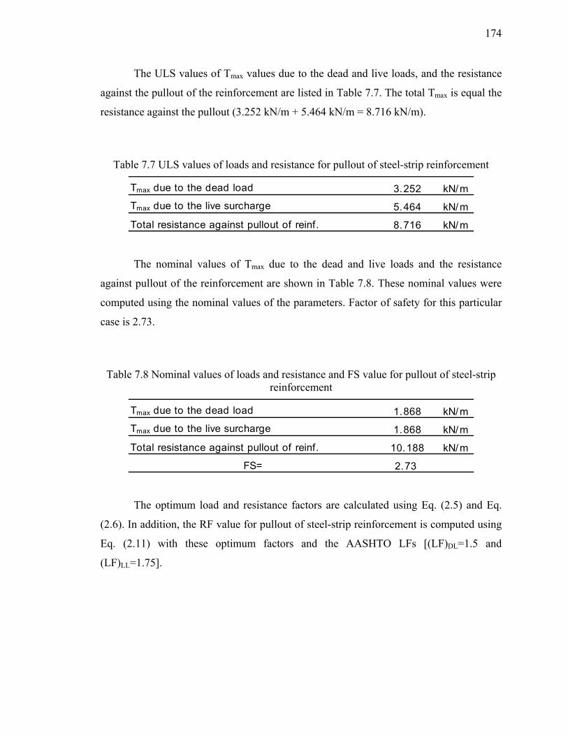
174
The ULS values of Tmax values due to the dead and live loads, and the resistance
against the pullout of the reinforcement are listed in Table 7.7. The total Tmax is equal the
resistance against the pullout (3.252 kN/m + 5.464 kN/m = 8.716 kN/m).
Table 7.7 ULS values of loads and resistance for pullout of steel-strip reinforcement
3.252 kN/m
5.464 kN/m
8.716 kN/m
Tmax due to the dead load
Tmax due to the live surcharge
Total resistance against pullout of reinf.
The nominal values of Tmax due to the dead and live loads and the resistance
against pullout of the reinforcement are shown in Table 7.8. These nominal values were
computed using the nominal values of the parameters. Factor of safety for this particular
case is 2.73.
Table 7.8 Nominal values of loads and resistance and FS value for pullout of steel-strip reinforcement
1.868 kN/m
1.868 kN/m
10.188 kN/m
2.73FS=
Tmax due to the dead load
Tmax due to the live surcharge
Total resistance against pullout of reinf.
The optimum load and resistance factors are calculated using Eq. (2.5) and Eq.
(2.6). In addition, the RF value for pullout of steel-strip reinforcement is computed using
Eq. (2.11) with these optimum factors and the AASHTO LFs [(LF)DL=1.5 and
(LF)LL=1.75].

175
Table 7.9 Calculation of optimum factors and RF using AASHTO LFs for pullout of steel-strip reinforcement
(LF)DL* = 1.74 (LF)DL = 1.5 (LF)DL
* / (LF)DL = 1.16(LF)LL
* = 2.93 (LF)LL = 1.75 (LF)LL* / (LF)LL = 1.67
RF* = 0.86 RF= 0.51 [(LF)DL
* and (LF)LL* are the optimum load factors for dead and live load, RF* is the
optimum resistance factor, (LF)DL and (LF)LL are the AASHTO load factors, and RF is the resistance factor]
From Figure 7.19 through Figure 7.24, the RF values for pullout of steel-strip
reinforcement are calculated for different reinforcement levels and different target
reliability index values. RF value increases with increasing reinforcement depth z from
the top of the MSE wall.
Regardless of MSE wall height, the minimum RF value is determined at the first
reinforcement layer from the top of the MSE wall. Given that there is 0.3m barrier to the
pavement grade, the depths of the first reinforcement layers from the top of MSE wall
were 0.45, 0.6, and 0.7 for the MSE walls for which vertical spacing is 0.3, 0.6, and 0.8m,
respectively.
The RF value is independent of the vertical or horizontal spacing (sv or sh) of
reinforcement (or the tributary area of the reinforcement) if the reinforcement depth z is
the same because, from Eq. (7.4), the ratio of the effective length Le to the tributary area
(sv × sh) was constant (Le changes in proportion to the change of the tributary area). In
other words, for a given reinforcement depth z, if the tributary area increases n times
larger than the initial tributary area, Le also changes n times larger than the initial Le
without changing the value of reliability index as well as RF. We could observe this from
the results of our analysis (compare Figure 7.19 with Figure 7.20, Figure 7.21 with Figure
7.22, and Figure 7.23 with Figure 7.24, respectively).
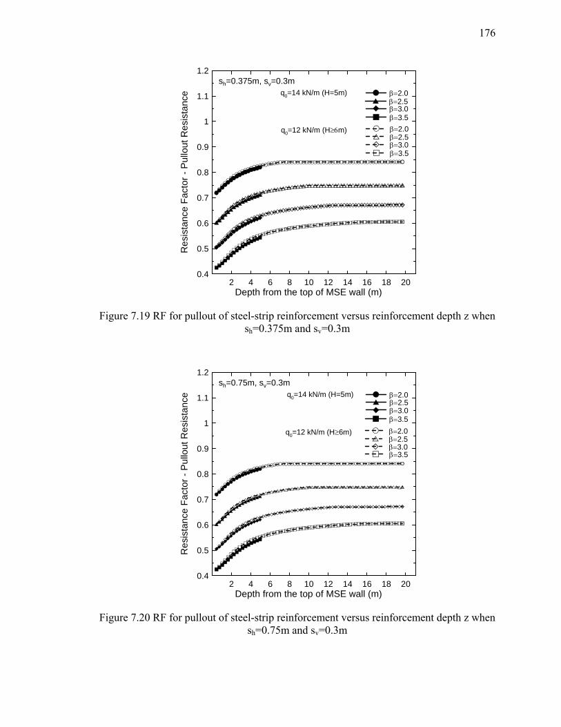
176
2 4 6 8 10 12 14 16 18 20Depth from the top of MSE wall (m)
0.4
0.5
0.6
0.7
0.8
0.9
1
1.1
1.2
Res
ista
nce
Fact
or -
Pul
lout
Res
ista
nce β=2.0
β=2.5β=3.0
q0=14 kN/m (H=5m)
β=2.0β=2.5β=3.0
q0=12 kN/m (H≥6m)
sh=0.375m, sv=0.3m
β=3.5
β=3.5
Figure 7.19 RF for pullout of steel-strip reinforcement versus reinforcement depth z when sh=0.375m and sv=0.3m
2 4 6 8 10 12 14 16 18 20Depth from the top of MSE wall (m)
0.4
0.5
0.6
0.7
0.8
0.9
1
1.1
1.2
Res
ista
nce
Fact
or -
Pul
lout
Res
ista
nce β=2.0
β=2.5β=3.0
q0=14 kN/m (H=5m)
β=2.0β=2.5β=3.0
q0=12 kN/m (H≥6m)
sh=0.75m, sv=0.3m
β=3.5
β=3.5
Figure 7.20 RF for pullout of steel-strip reinforcement versus reinforcement depth z when sh=0.75m and sv=0.3m

177
2 4 6 8 10 12 14 16 18 20Depth from the top of MSE wall (m)
0.4
0.5
0.6
0.7
0.8
0.9
1
1.1
1.2
Res
ista
nce
Fact
or -
Pul
lout
Res
ista
nce β=2.0
β=2.5β=3.0
q0=14 kN/m (H=5m)
β=2.0β=2.5β=3.0
q0=12 kN/m (H≥6m)
sh=0.375m, sv=0.6m
β=3.5
β=3.5
Figure 7.21 RF for pullout of steel-strip reinforcement versus reinforcement depth z when sh=0.375m and sv=0.6m
2 4 6 8 10 12 14 16 18 20Depth from the top of MSE wall (m)
0.4
0.5
0.6
0.7
0.8
0.9
1
1.1
1.2
Res
ista
nce
Fact
or -
Pul
lout
Res
ista
nce β=2.0
β=2.5β=3.0
q0=14 kN/m (H=5m)
β=2.0β=2.5β=3.0
q0=12 kN/m (H≥6m)
sh=0.75m, sv=0.6m
β=3.5
β=3.5
Figure 7.22 RF for pullout of steel-strip reinforcement versus reinforcement depth z when sh=0.75m and sv=0.6m

178
2 4 6 8 10 12 14 16 18 20Depth from the top of MSE wall (m)
0.4
0.5
0.6
0.7
0.8
0.9
1
1.1
1.2
Res
ista
nce
Fact
or -
Pul
lout
Res
ista
nce β=2.0
β=2.5β=3.0
q0=14 kN/m (H=5m)
β=2.0β=2.5β=3.0
q0=12 kN/m (H≥6m)
sh=0.375m, sv=0.8m
β=3.5
β=3.5
Figure 7.23 RF for pullout of steel-strip reinforcement versus reinforcement depth z when sh=0.375m and sv=0.8m
2 4 6 8 10 12 14 16 18 20Depth from the top of MSE wall (m)
0.4
0.5
0.6
0.7
0.8
0.9
1
1.1
1.2
Res
ista
nce
Fact
or -
Pul
lout
Res
ista
nce β=2.0
β=2.5β=3.0
q0=14 kN/m (H=5m)
β=2.0β=2.5β=3.0
q0=12 kN/m (H≥6m)
sh=0.75m, sv=0.8m
β=3.5
β=3.5
Figure 7.24 RF for pullout of steel-strip reinforcement versus reinforcement depth z when sh=0.75m and sv=0.8m

179
In order to explain the relationship between the RF value and the reinforcement
depth z from the top of the MSE walls in Figure 7.19 through Figure 7.24, we should
examine the changes of the optimum factors (optimum LFs for dead load and live load
and optimum resistance factor) with increasing z. Therefore, RF values of a particular
case (sv=0.60m, H=20m, βT=3.0, and q0=12 kN/m) were studied. As shown in Figure
7.25, the following is observed: (1) the optimum resistance factor RF* maintains
somewhat consistent level with increasing z, (2) the optimum load factor LF*DL for the
dead load increases slightly with increasing z and (3) the optimum load factor LF*LL for
the live load decreases substantially at lower reinforcement depth z and slowly converge
to a certain value with increasing z.
0 5 10 15 20Depth from the top of MSE wall (m)
0.00
0.50
1.00
1.50
2.00
2.50
3.00
Opt
imum
fact
ors
(LF)DL*(LF)LL*RF*
Figure 7.25 Changes of optimum factors (resistance factor, load factors for live load and dead load) with an increasing reinforcement depth from the top of MSE wall (sv=0.60m, H=20m, βT=3.0, and q0=12 kN/m) [(LF)DL
* and (LF)LL* are the optimum load factors for
dead and live load, and RF* is the optimum resistance factor]

180
As mentioned in section 7.3, the LFs in AASHTO LRFD specifications (2007) for
pullout of steel-strip reinforcement are 1.5 and 1.75 for dead load and live load,
respectively [(LF)DL=1.5 and (LF)LL=1.75]. The RF value (Eq. (2.11)) can be expressed
as
( )( )
( )( )
*
* *
DL LL
DL LL
RFRFLF LF
max ,LF LF
=⎛ ⎞⎜ ⎟⎜ ⎟⎝ ⎠
(7.19)
Figure 7.26 represents the changes of the ratios of (LF)DL*/(LF)DL and
(LF)LL*/(LF)LL and RF* with increasing reinforcement depth z from the top of MSE wall.
The following explains the reason why RF value increases rapidly at a lower z and
maintains at a consistent level after a certain depth z: RF* value does not change
significantly with increasing reinforcement depth z while (LF)DL*/(LF)DL and
(LF)LL*/(LF)LL vary with z. Therefore, the change in RF value with increasing z is mainly
due to the change of the higher values between (LF)DL*/(LF)DL and (LF)LL
*/(LF)LL. At a
lower depth z, (LF)LL*/(LF)LL is much more higher than (LF)DL
*/(LF)DL and decreases
rapidly; However, after a certain reinforcement depth (in this particular case, z greater
than 10m), the higher value between (LF)LL*/(LF)LL and (LF)DL
*/(LF)DL maintains
somewhat consistent level, and therefore RF value also remains consistent.

181
0 5 10 15 20Depth from the top of MSE wall (m)
0.75
1.00
1.25
1.50
1.75
RF*
, (L
F)D
L*/(L
F)D
L, (L
F)LL
*/(L
F)LL
(LF)DL*/(LF)DL
(LF)LL*/(LF)LL
RF*
Figure 7.26 Changes of RF*, (LF)DL*/(LF)DL, and (LF)LL
*/(LF)LL with increasing reinforcement depth z (sv=0.60m, H=20m, βT=3.0, and q0=12 kN/m) [(LF)DL
* and (LF)LL
* are the optimum load factors for dead and live load, RF* is the optimum resistance factor, and (LF)DL and (LF)LL are the AASHTO load factors]
FS values are calculated using the load and resistance equations proposed in this
report. The FS values in Figure 7.27 through Figure 7.32 are the values that correspond to
the RF values in Figure 7.19 through Figure 7.24. It is also noticed earlier that FS value is
independent of horizontal and vertical spacing of the reinforcement for a given
reinforcement level. The FS value is the highest at the first reinforcement depth z and
continuously decreases with increasing z. This trend of FS is opposite to that of RF. This
is because higher FS value in design allows more margin of safety to the structure; while
lower RF value in design assumes less probability of failure of the structure.

182
2 4 6 8 10 12 14 16 18 20Depth from the top of MSE wall (m)
1.5
1.7
1.9
2.1
2.3
2.5
2.7
2.9
3.1
3.3
3.5
Fact
or o
f Saf
ety
- Pul
lout
Res
ista
nce β=2.0
β=2.5β=3.0
q0=14 kN/m (H=5m)
β=2.0β=2.5β=3.0
q0=12 kN/m (H≥6m)
sh=0.375m, sv=0.3m
β=3.5
β=3.5
Figure 7.27 FS for pullout of steel-strip reinforcement versus reinforcement depth z when sh=0.375m and sv=0.3m
2 4 6 8 10 12 14 16 18 20Depth from the top of MSE wall (m)
1.5
1.7
1.9
2.1
2.3
2.5
2.7
2.9
3.1
3.3
3.5
Fact
or o
f Saf
ety
- Pul
lout
Res
ista
nce β=2.0
β=2.5β=3.0
q0=14 kN/m (H=5m)
β=2.0β=2.5β=3.0
q0=12 kN/m (H≥6m)
sh=0.75m, sv=0.3m
β=3.5
β=3.5
Figure 7.28 FS for pullout of steel-strip reinforcement versus reinforcement depth z when sh=0.75m and sv=0.3m

183
2 4 6 8 10 12 14 16 18 20Depth from the top of MSE wall (m)
1.5
1.7
1.9
2.1
2.3
2.5
2.7
2.9
3.1
3.3
3.5
Fact
or o
f Saf
ety
- Pul
lout
Res
ista
nce β=2.0
β=2.5β=3.0
q0=14 kN/m (H=5m)
β=2.0β=2.5β=3.0
q0=12 kN/m (H≥6m)
sh=0.375m, sv=0.6m
β=3.5
β=3.5
Figure 7.29 FS for pullout of steel-strip reinforcement versus reinforcement depth z when sh=0.375m and sv=0.6m
2 4 6 8 10 12 14 16 18 20Depth from the top of MSE wall (m)
1.5
1.7
1.9
2.1
2.3
2.5
2.7
2.9
3.1
3.3
3.5
Fact
or o
f Saf
ety
- Pul
lout
Res
ista
nce β=2.0
β=2.5β=3.0
q0=14 kN/m (H=5m)
β=2.0β=2.5β=3.0
q0=12 kN/m (H≥6m)
sh=0.75m, sv=0.6m
β=3.5
β=3.5
Figure 7.30 FS for pullout of steel-strip reinforcement versus reinforcement depth z when sh=0.75m and sv=0.6m

184
2 4 6 8 10 12 14 16 18 20Depth from the top of MSE wall (m)
1.5
1.7
1.9
2.1
2.3
2.5
2.7
2.9
3.1
3.3
3.5
Fact
or o
f Saf
ety
- Pul
lout
Res
ista
nce β=2.0
β=2.5β=3.0
q0=14 kN/m (H=5m)
β=2.0β=2.5β=3.0
q0=12 kN/m (H≥6m)
sh=0.375m, sv=0.8m
β=3.5
β=3.5
Figure 7.31 FS for pullout of steel-strip reinforcement versus reinforcement depth z when sh=0.375m and sv=0.8m
2 4 6 8 10 12 14 16 18 20Depth from the top of MSE wall (m)
1.5
1.7
1.9
2.1
2.3
2.5
2.7
2.9
3.1
3.3
3.5
Fact
or o
f Saf
ety
- Pul
lout
Res
ista
nce β=2.0
β=2.5β=3.0
q0=14 kN/m (H=5m)
β=2.0β=2.5β=3.0
q0=12 kN/m (H≥6m)
sh=0.75m, sv=0.8m
β=3.5
β=3.5
Figure 7.32 FS for pullout of steel-strip reinforcement versus reinforcement depth z when sh=0.75m and sv=0.8m

185
According to the FHWA (2001) and AASHTO (2007) specifications, the FS for
pullout of reinforcement criterion should be equal to or higher than 1.5. However, the FS
values that are achieved from all the analyses in these examples are higher than 1.5 (the
smallest FS value is about 1.8). The reasons for having higher FS values than 1.5 are as
follows: (1) there exists a higher uncertainty associated with assessing Kr and (2) the
existing design methods [FHWA (2001) and AASHTO (2007)] overestimate Kr so that
the FS values provided in these design specifications may be much higher if the
estimation of Kr has done more realistic or reasonable.
7.6.2. Structural failure of steel-strip reinforcement
The distribution of resistance (the yield force Ty of a steel-strip reinforcement) does not
change with its location. On contrary, the maximum tensile force Tmax on the steel-strip
reinforcement changes with its location (reinforcement depth). We performed reliability
analyses for every reinforcement depth z (up to 20m) using the Microsoft Excel Solver.
When the horinzontal spacing was 0.375m, regardless of the vertical spacing
(sv=0.3-0.8m), all the calculated reliability indices were higher than the highest target
reliability index (βT=3.5) for all the reinforcement depths up to 20m. For sh = 0.75m,
when vertical spacing is equal to or less than 0.4m, all the calculated reliability indices
were higher than the highest target reliability index (βT=3.5).
Figure 7.33 shows the calculated reliability indices for sh = 0.75m and sv = 0.4, 0.5,
0.6, 0.7, and 0.8m. For given horizontal and vertical spacings of the reinforcement, the
reliability index decreases with increasing steel-strip reinforcement depth. This is because
the maximum tensile force Tmax on the steel-strip reinforcement increases with increasing
reinforcement depth, while the resistance does not change with respect to reinforcement
depth; therefore, the probability of failure increases with increasing reinforcement depth.
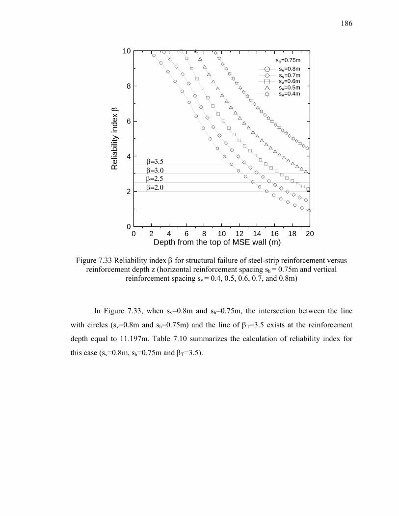
186
0 2 4 6 8 10 12 14 16 18 20Depth from the top of MSE wall (m)
0
2
4
6
8
10
Rel
iabi
lity
inde
x β
sv=0.8msv=0.7msv=0.6msv=0.5msv=0.4m
β=3.5β=3.0β=2.5β=2.0
sh=0.75m
Figure 7.33 Reliability index β for structural failure of steel-strip reinforcement versus reinforcement depth z (horizontal reinforcement spacing sh = 0.75m and vertical
reinforcement spacing sv = 0.4, 0.5, 0.6, 0.7, and 0.8m)
In Figure 7.33, when sv=0.8m and sh=0.75m, the intersection between the line
with circles (sv=0.8m and sh=0.75m) and the line of βT=3.5 exists at the reinforcement
depth equal to 11.197m. Table 7.10 summarizes the calculation of reliability index for
this case (sv=0.8m, sh=0.75m and βT=3.5).

187
Table 7.10 Result of reliability analysis for structural failure of steel-strip reinforcement (sv=0.8m, sh=0.75m and βT=3.5)
m equivalentnormal mean x stdev equivalent
normal stdevKr 0.196 0.196 0.42 0.068 0.068 0.0046 0.0000 0.0000 0.0000γrf 20 20 20.06 0.24 0.240 0.0000 0.0576 0.0000 0.0000
q0,rf 13.8 14.354 14.43 3.45 0.246 0.0000 0.0000 0.0605 0.0000η(fy) 1 1 0.95 0.05 0.050 0.0000 0.0000 0.0000 0.0025
G(x) 0 11.197 m λ 2.594β 3.500 ζ 0.246Pf 0.0002
Reinforcement depth =
Covariance matrix, C
(m: mean value, stdev: standard deviation, G(x): function of margin of safety, β: reliability index, Pf: target probability of failure, λ and ζ are the parameters related to lognormal distribution, and η(fy) denotes a parameter that accounts the bias factor and coefficient of variation of the yield strength of the steel-strip reinforcement)
The ULS values of Tmax values due to the dead and live loads, and the yield force
of the steel-strip reinforcement are listed in Table 7.11. The total Tmax is equal the yield
force of the reinforcement (75.791 kN/m + 4.870 kN/m = 80.661 kN/m).
Table 7.11 ULS values of loads and resistance for structural failure of steel-strip reinforcement
Tmax due to the dead load 75.791 kN/mTmax due to the live surcharge 4.870 kN/mYield force of reinforcement 80.661 kN/m
The nominal values of Tmax values due to the dead and live loads, and the yield
force of the reinforcement are shown in Table 7.12. These nominal values were computed
using the nominal values of the parameters. Factor of safety for this particular case is
2.28.

188
Table 7.12 Nominal values of loads and resistance and FS value for structural failure of steel-strip reinforcement
Tmax due to the dead load 35.198 kN/mTmax due to the live surcharge 2.169 kN/mYield force of reinforcement 85.272 kN/m
FS= 2.28
The optimum load and resistance factors are calculated using Eq. (2.5) and Eq.
(2.6). In addition, the RF value for structural failure of steel-strip reinforcement is
computed using Eq. (2.11) with these optimum factors and the AASHTO LFs
[(LF)DL=1.5 and (LF)LL=1.75].
Table 7.13 Calculation of optimum factors and RF using AASHTO LFs for structural failure of steel-strip reinforcement
(LF)DL* = 2.15 (LF)DL= 1.5 (LF)DL
* / (LF)DL= 1.44(LF)LL
* = 2.25 (LF)LL= 1.75 (LF)LL* / (LF)LL= 1.28
RF* = 0.95 RF= 0.66 [(LF)DL
* and (LF)LL* are the optimum load factors for dead and live load, RF* is the
optimum resistance factor, (LF)DL and (LF)LL are the AASHTO load factors, and RF is the resistance factor]
RF values and the corresponding reinforcement levels are listed in Table 7.14 for
the intersection points (Figure 7.33) between the lines that consist of the calculated
reliability indices and the lines corresponding to the target reliability indices (βT = 2.0,
2.5, 3.0, and 3.5).

189
Table 7.14 RF and the corresponding reinforcement level for different target reliability indices (sh = 0.75m)
Vertical spacing, sv
(m)
RF & Reinf. level
Target reliability index, βT
3.5 3 2.5 2
0.8 RF 0.66 0.72 0.79 0.87
Reinf. level (m) 11.20 12.30 13.59 15.13
0.7 RF 0.66 0.72 0.79 0.87
Reinf. level (m) 12.90 14.15 15.63 17.39
0.6 RF 0.66 0.72 0.79 -
Reinf. level (m) 15.17 16.63 18.35 -
0.5 RF 0.66 - - -
Reinf. level (m) 18.34 - - -
From inequality (2.2), if the factored resistance is not equal to or greater than the
sum of the factored loads, designers should reduce either the horizontal or vertical
spacing of the reinforcements until the inequality (2.2) is satisfied.
Table 7.15 shows the FS values for the different target reliability indices. The FS
value for working stress design (WSD) is 1.8 (the inverse of 0.55). Because we are using
different method to assess the maximum tensile force Tmax compared to the method given
in the specifications (FHWA, 2001), the direct comparison between these FS values is
not possible.
Table 7.15 FS for different target reliability indices (sh = 0.75m)
Vertical spacing, sv
(m)
Target reliability index, βT
3.5 3 2.5 2
0.8 2.28 2.09 1.90 1.71
0.7 2.28 2.09 1.90 1.71
0.6 2.28 2.09 1.90 -
0.5 2.28 - - -

190
CHAPTER 8. PARAMETRIC STUDY
The goal of this chapter is to determine the RF values for each stability limit state (both
external and internal) using the LF values provided in AASHTO (2007). Before
determining the RF values, we will examine the effect on the RF of each parameter used
in the analysis. To observe these effects, sets of parametric studies were performed.
The equations for loads and resistance calculations in our design method are
different from those in the specifications (AASHTO, 2007 and FHWA, 2001). Therefore,
to use the RF values proposed in this study, designers must use the equations for load and
resistance that are proposed in this study. For example, we used the critical-state friction
angle to estimate the active earth pressure coefficient KA, while the method in the
specifications uses the peak friction angle for KA estimation.
8.1. Effect of the Change in the Critical-State Friction Angle of Retained Soil on RF
The critical-state friction angle of the retained soil φc,rt affects only the RFs for sliding
and overturning because φc,rt is not used in the internal stability ULS equations. To see
the effect of φc,rt on RF, analyses were performed using two different values of φc,rt (30°
and 33°) fixing the values of the other parameters.
8.1.1. External stability – sliding
The RF value for sliding was investigated for two different values of φc,rt (30° and 33°),
as shown in Figure 8.1. The result shows that the RF values for φc,rt was 33° are slightly
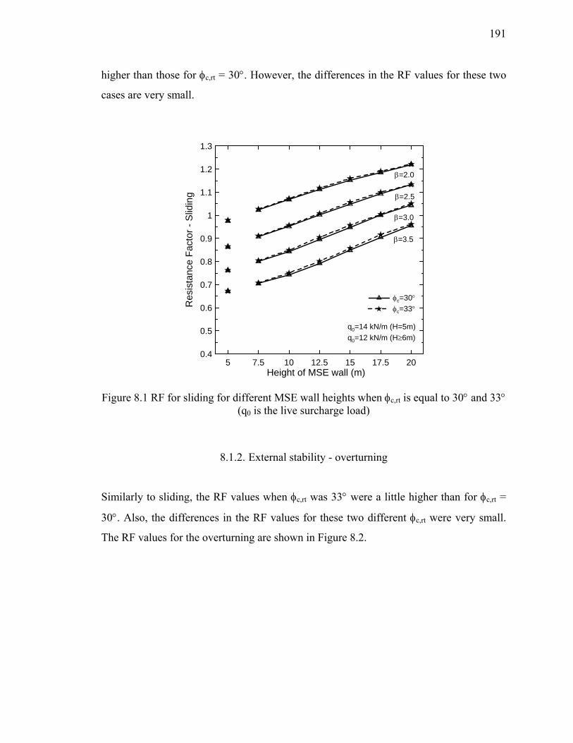
191
higher than those for φc,rt = 30°. However, the differences in the RF values for these two
cases are very small.
5 7.5 10 12.5 15 17.5 20Height of MSE wall (m)
0.4
0.5
0.6
0.7
0.8
0.9
1
1.1
1.2
1.3
Res
ista
nce
Fact
or -
Slid
ing
φc=30°
q0=12 kN/m (H≥6m)q0=14 kN/m (H=5m)
φc=33°
β=2.0
β=2.5
β=3.0
β=3.5
Figure 8.1 RF for sliding for different MSE wall heights when φc,rt is equal to 30° and 33° (q0 is the live surcharge load)
8.1.2. External stability - overturning
Similarly to sliding, the RF values when φc,rt was 33° were a little higher than for φc,rt =
30°. Also, the differences in the RF values for these two different φc,rt were very small.
The RF values for the overturning are shown in Figure 8.2.
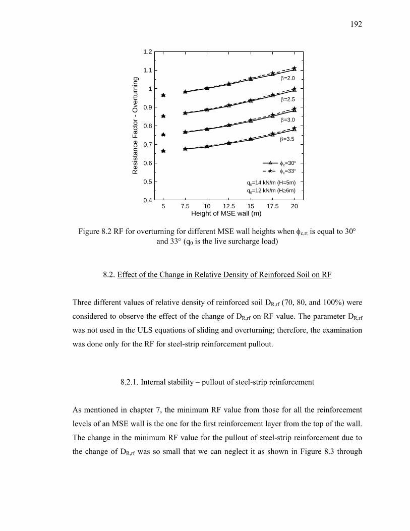
192
5 7.5 10 12.5 15 17.5 20Height of MSE wall (m)
0.4
0.5
0.6
0.7
0.8
0.9
1
1.1
1.2
Res
ista
nce
Fact
or -
Ove
rturn
ing
φc=30°
q0=12 kN/m (H≥6m)q0=14 kN/m (H=5m)
φc=33°
β=2.0
β=2.5
β=3.0
β=3.5
Figure 8.2 RF for overturning for different MSE wall heights when φc,rt is equal to 30° and 33° (q0 is the live surcharge load)
8.2. Effect of the Change in Relative Density of Reinforced Soil on RF
Three different values of relative density of reinforced soil DR,rf (70, 80, and 100%) were
considered to observe the effect of the change of DR,rf on RF value. The parameter DR,rf
was not used in the ULS equations of sliding and overturning; therefore, the examination
was done only for the RF for steel-strip reinforcement pullout.
8.2.1. Internal stability – pullout of steel-strip reinforcement
As mentioned in chapter 7, the minimum RF value from those for all the reinforcement
levels of an MSE wall is the one for the first reinforcement layer from the top of the wall.
The change in the minimum RF value for the pullout of steel-strip reinforcement due to
the change of DR,rf was so small that we can neglect it as shown in Figure 8.3 through

193
Figure 8.5, which also show a tendency of the minimum RF to decrease as the DR,rf
increases.
70 80 90 100Relative Density of Reinforced Soil, DR,rf (%)
0.3
0.4
0.5
0.6
0.7
0.8
Min
ium
Res
ista
nce
Fact
or -
Pul
lout
Res
ista
nce
β=2.0β=2.5β=3.0
sv=0.3m, sh=0.375m orsv=0.3m, sh=0.75m
q0=14 kN/m (H=5m) q0=12 kN/m (H≥6m)β=2.0β=2.5β=3.0
β=3.5 β=3.5
Figure 8.3 Minimum RF for pullout of steel-strip reinforcement for different values of DR,rf when sv=0.3m (q0 is the live surcharge load)
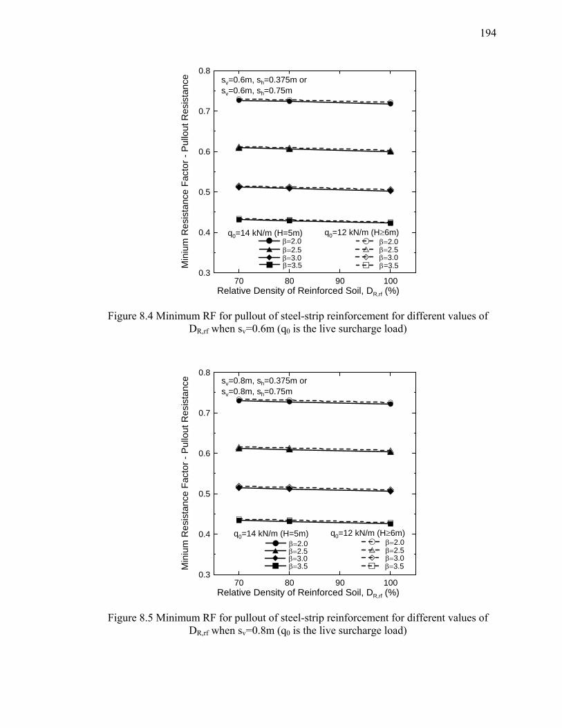
194
70 80 90 100Relative Density of Reinforced Soil, DR,rf (%)
0.3
0.4
0.5
0.6
0.7
0.8
Min
ium
Res
ista
nce
Fact
or -
Pul
lout
Res
ista
nce
β=2.0β=2.5β=3.0
sv=0.6m, sh=0.375m or sv=0.6m, sh=0.75m
q0=14 kN/m (H=5m) q0=12 kN/m (H≥6m)β=2.0β=2.5β=3.0
β=3.5 β=3.5
Figure 8.4 Minimum RF for pullout of steel-strip reinforcement for different values of DR,rf when sv=0.6m (q0 is the live surcharge load)
70 80 90 100Relative Density of Reinforced Soil, DR,rf (%)
0.3
0.4
0.5
0.6
0.7
0.8
Min
ium
Res
ista
nce
Fact
or -
Pul
lout
Res
ista
nce
β=2.0β=2.5β=3.0
sv=0.8m, sh=0.375m or sv=0.8m, sh=0.75m
q0=14 kN/m (H=5m) q0=12 kN/m (H≥6m)β=2.0β=2.5β=3.0
β=3.5 β=3.5
Figure 8.5 Minimum RF for pullout of steel-strip reinforcement for different values of DR,rf when sv=0.8m (q0 is the live surcharge load)
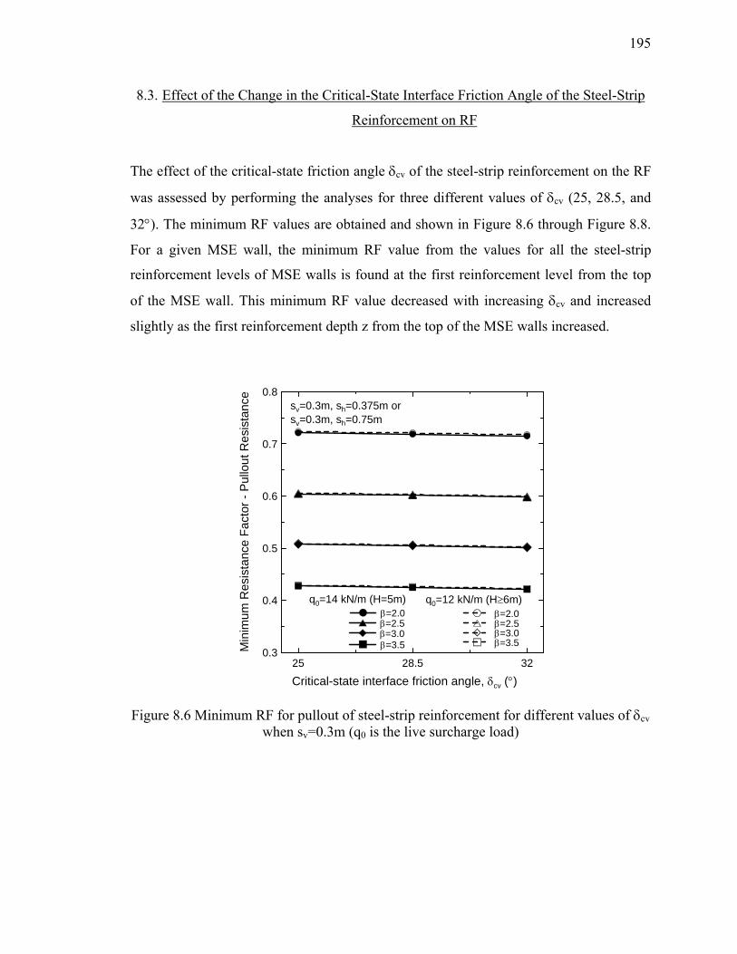
195
8.3. Effect of the Change in the Critical-State Interface Friction Angle of the Steel-Strip
Reinforcement on RF
The effect of the critical-state friction angle δcv of the steel-strip reinforcement on the RF
was assessed by performing the analyses for three different values of δcv (25, 28.5, and
32°). The minimum RF values are obtained and shown in Figure 8.6 through Figure 8.8.
For a given MSE wall, the minimum RF value from the values for all the steel-strip
reinforcement levels of MSE walls is found at the first reinforcement level from the top
of the MSE wall. This minimum RF value decreased with increasing δcv and increased
slightly as the first reinforcement depth z from the top of the MSE walls increased.
25 28.5 32
Critical-state interface friction angle, δcv (°)
0.3
0.4
0.5
0.6
0.7
0.8
Min
imum
Res
ista
nce
Fact
or -
Pul
lout
Res
ista
nce
β=2.0β=2.5β=3.0
q0=14 kN/m (H=5m)
sv=0.3m, sh=0.375m orsv=0.3m, sh=0.75m
q0=12 kN/m (H≥6m)β=2.0β=2.5β=3.0
β=3.5 β=3.5
Figure 8.6 Minimum RF for pullout of steel-strip reinforcement for different values of δcv when sv=0.3m (q0 is the live surcharge load)

196
25 28.5 32
Critical-state interface friction angle, δcv (°)
0.3
0.4
0.5
0.6
0.7
0.8
Min
imum
Res
ista
nce
Fact
or -
Pul
lout
Res
ista
nce
β=2.0β=2.5β=3.0
q0=14 kN/m (H=5m)
sv=0.6m, sh=0.375m orsv=0.6m, sh=0.75m
q0=12 kN/m (H≥6m)β=2.0β=2.5β=3.0
β=3.5 β=3.5
Figure 8.7 Minimum RF for pullout of steel-strip reinforcement for different values of δcv when sv=0.6m (q0 is the live surcharge load)
25 28.5 32
Critical-state interface friction angle, δcv (°)
0.3
0.4
0.5
0.6
0.7
0.8
Min
imum
Res
ista
nce
Fact
or -
Pul
lout
Res
ista
nce
β=2.0β=2.5β=3.0
q0=14 kN/m (H=5m)
sv=0.8m, sh=0.375m orsv=0.8m, sh=0.75m
q0=12 kN/m (H≥6m)β=2.0β=2.5β=3.0
β=3.5 β=3.5
Figure 8.8 Minimum RF for pullout of steel-strip reinforcement for different values of δcv when sv=0.8m (q0 is the live surcharge load)
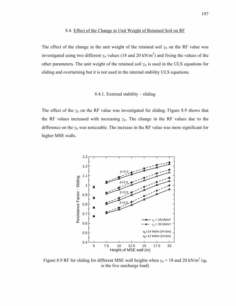
197
8.4. Effect of the Change in Unit Weight of Retained Soil on RF
The effect of the change in the unit weight of the retained soil γrt on the RF value was
investigated using two different γrt values (18 and 20 kN/m3) and fixing the values of the
other parameters. The unit weight of the retained soil γrt is used in the ULS equations for
sliding and overturning but it is not used in the internal stability ULS equations.
8.4.1. External stability – sliding
The effect of the γrt on the RF value was investigated for sliding. Figure 8.9 shows that
the RF values increased with increasing γrt. The change in the RF values due to the
difference on the γrt was noticeable. The increase in the RF value was more significant for
higher MSE walls.
5 7.5 10 12.5 15 17.5 20Height of MSE wall (m)
0.4
0.5
0.6
0.7
0.8
0.9
1
1.1
1.2
1.3
Res
ista
nce
Fact
or -
Slid
ing
γrt = 18 kN/m3
q0=12 kN/m (H≥6m)q0=14 kN/m (H=5m)
γrt = 20 kN/m3
β=2.0
β=2.5
β=3.0
β=3.5
Figure 8.9 RF for sliding for different MSE wall heights when γrt = 18 and 20 kN/m3 (q0 is the live surcharge load)
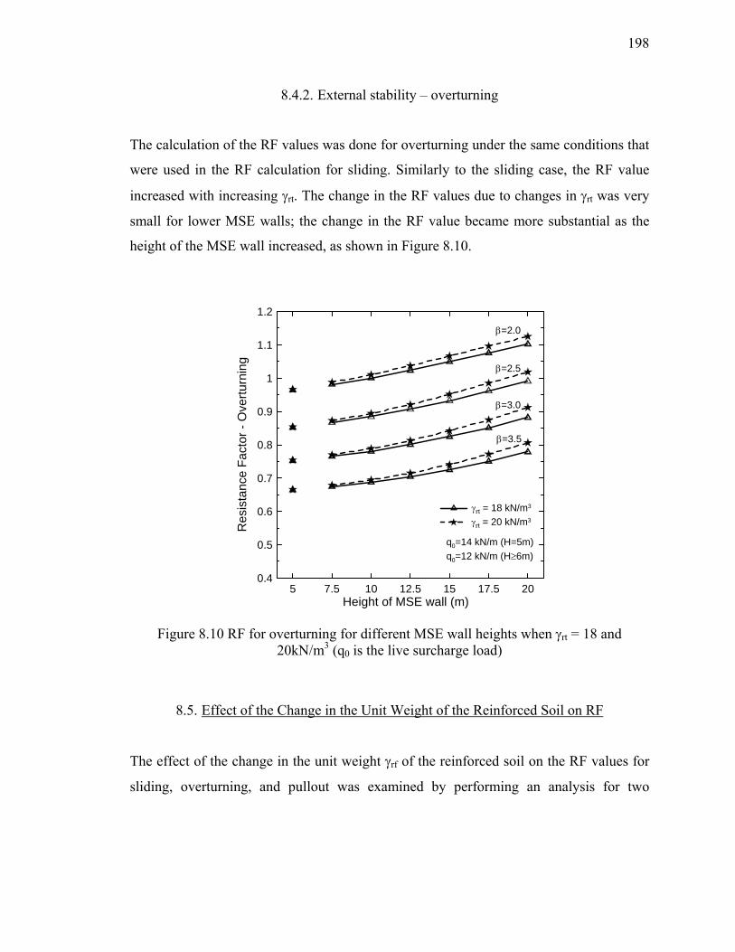
198
8.4.2. External stability – overturning
The calculation of the RF values was done for overturning under the same conditions that
were used in the RF calculation for sliding. Similarly to the sliding case, the RF value
increased with increasing γrt. The change in the RF values due to changes in γrt was very
small for lower MSE walls; the change in the RF value became more substantial as the
height of the MSE wall increased, as shown in Figure 8.10.
5 7.5 10 12.5 15 17.5 20Height of MSE wall (m)
0.4
0.5
0.6
0.7
0.8
0.9
1
1.1
1.2
Res
ista
nce
Fact
or -
Ove
rturn
ing
γrt = 18 kN/m3
q0=12 kN/m (H≥6m)q0=14 kN/m (H=5m)
γrt = 20 kN/m3
β=2.0
β=2.5
β=3.0
β=3.5
Figure 8.10 RF for overturning for different MSE wall heights when γrt = 18 and 20kN/m3 (q0 is the live surcharge load)
8.5. Effect of the Change in the Unit Weight of the Reinforced Soil on RF
The effect of the change in the unit weight γrf of the reinforced soil on the RF values for
sliding, overturning, and pullout was examined by performing an analysis for two

199
different values of γrf (20 and 22 kN/m3), fixing the values of the other parameters. The
effect of the change in γrf on RF for each criterion was insignificant.
8.5.1. External stability – sliding
The effect of the change in γrf on the RF for sliding was negligible, as shown in Figure
8.11. The RF values for the higher γrf (22 kN/m3) were slightly higher than those for the
lower γrf (20 kN/m3).
5 7.5 10 12.5 15 17.5 20Height of MSE wall (m)
0.4
0.5
0.6
0.7
0.8
0.9
1
1.1
1.2
1.3
Res
ista
nce
Fact
or -
Slid
ing
γrf = 20 kN/m3
q0=12 kN/m (H≥6m)q0=14 kN/m (H=5m)
γrf = 22 kN/m3
β=2.0
β=2.5
β=3.0
β=3.5
Figure 8.11 RF for sliding for different MSE wall heights when γrf = 20 and 22 kN/m3 (q0 is the live surcharge load)
8.5.2. External stability – overturning

200
Similarly to sliding, the RF values did change significantly due to the change in γrf, as
shown in Figure 8.12. There was an insignificant increase in the RF value when the γrf
changed from 20 to 22 kN/m3.
5 7.5 10 12.5 15 17.5 20Height of MSE wall (m)
0.4
0.5
0.6
0.7
0.8
0.9
1
1.1
1.2R
esis
tanc
e Fa
ctor
- O
vertu
rnin
g
γrf = 20 kN/m3
q0=12 kN/m (H≥6m)q0=14 kN/m (H=5m)
γrf = 22 kN/m3
β=2.0
β=2.5
β=3.0
β=3.5
Figure 8.12 RF for overturning for different MSE wall heights when γrf = 20 and 22 kN/m3 (q0 is the live surcharge load)
8.5.3. Internal stability – steel-strip reinforcement pullout
The effect of the unit weight γrf of the reinforced soil on the minimum RF value was also
insignificant for pullout of the steel-strip reinforcement, as illustrated in Figure 8.13 and
Figure 8.14. For a given reinforcement level, the RF value increased slightly with
increasing γrf.
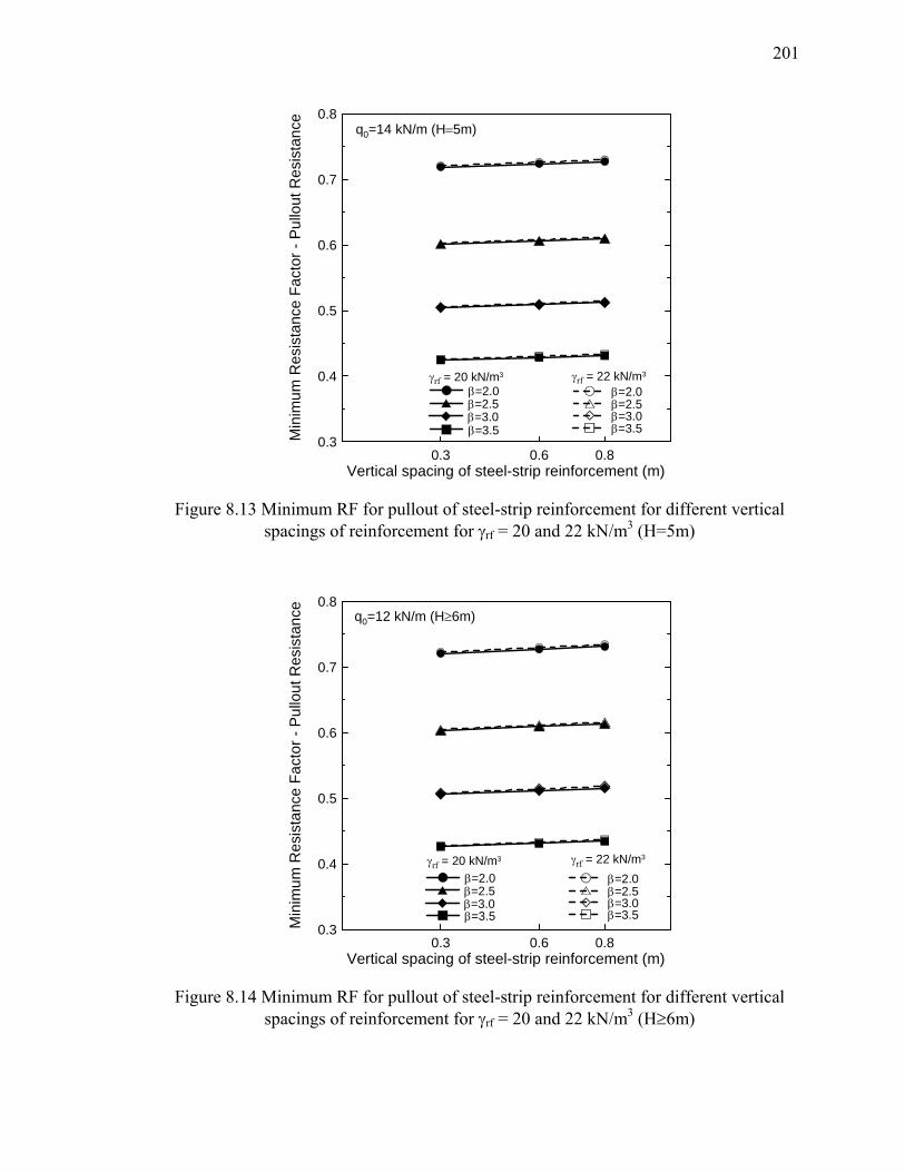
201
Vertical spacing of steel-strip reinforcement (m)
0.3
0.4
0.5
0.6
0.7
0.8
Min
imum
Res
ista
nce
Fact
or -
Pul
lout
Res
ista
nce
β=2.0β=2.5β=3.0
q0=14 kN/m (H=5m)
0.3
β=2.0
0.6
β=2.5
0.8
β=3.0
γrf = 20 kN/m3 γrf = 22 kN/m3
β=3.5 β=3.5
Figure 8.13 Minimum RF for pullout of steel-strip reinforcement for different vertical spacings of reinforcement for γrf = 20 and 22 kN/m3 (H=5m)
Vertical spacing of steel-strip reinforcement (m)
0.3
0.4
0.5
0.6
0.7
0.8
Min
imum
Res
ista
nce
Fact
or -
Pul
lout
Res
ista
nce
β=2.0β=2.5β=3.0
γrf = 20 kN/m3
q0=12 kN/m (H≥6m)
0.3
β=2.0
0.6
β=2.5
0.8
β=3.0
γrf = 22 kN/m3
β=3.5 β=3.5
Figure 8.14 Minimum RF for pullout of steel-strip reinforcement for different vertical spacings of reinforcement for γrf = 20 and 22 kN/m3 (H≥6m)
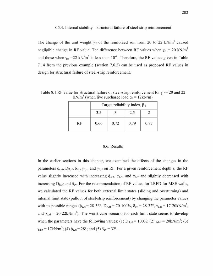
202
8.5.4. Internal stability – structural failure of steel-strip reinforcement
The change of the unit weight γrf of the reinforced soil from 20 to 22 kN/m3 caused
negligible change in RF value. The difference between RF values when γrf = 20 kN/m3
and those when γrf =22 kN/m3 is less than 10-4. Therefore, the RF values given in Table
7.14 from the previous example (section 7.6.2) can be used as proposed RF values in
design for structural failure of steel-strip reinforcement.
Table 8.1 RF value for structural failure of steel-strip reinforcement for γrf = 20 and 22 kN/m3 (when live surcharge load q0 = 12kN/m)
Target reliability index, βT
3.5 3 2.5 2
RF 0.66 0.72 0.79 0.87
8.6. Results
In the earlier sections in this chapter, we examined the effects of the changes in the
parameters φc,rt, DR,rf, δcv, γd,rt, and γd,rf on RF. For a given reinforcement depth z, the RF
value slightly increased with increasing φc,rt, γd,rt, and γd,rf and slightly decreased with
increasing DR,rf and δcv. For the recommendation of RF values for LRFD for MSE walls,
we calculated the RF values for both external limit states (sliding and overturning) and
internal limit state (pullout of steel-strip reinforcement) by changing the parameter values
with its possible ranges (φc,rt = 28-36°, DR,rf = 70-100%, δcv = 28-32°, γd,rt = 17-20kN/m3,
and γd,rf = 20-22kN/m3). The worst case scenario for each limit state seems to develop
when the parameters have the following values: (1) DR,rf = 100%; (2) γd,rf = 20kN/m3; (3)
γd,rt = 17kN/m3; (4) φc,rt = 28°; and (5) δcv = 32°.

203
RF values of the worst case scenario for each limit state are compared with those
values calculated in the examples in chapter 6 and chapter 7. The RF values of the worst
case scenario for each limit state could be proposed as the recommended RFs for LRFD
for MSE walls when the design is done following all the proposed method in this report.
8.6.1. External stability – sliding
Both the RF values for sliding calculated in the example in chapter 6 and those of the
worst case scenario increased with increasing MSE wall height and decreasing target
reliability index. However, the difference in the RF value between these two cases
increases with an increasing height of the MSE walls as shown in Figure 8.15.
5 7.5 10 12.5 15 17.5 20Height of MSE wall (m)
0.4
0.5
0.6
0.7
0.8
0.9
1
1.1
1.2
1.3
Res
ista
nce
Fact
or -
Slid
ing
RF values calculated in the examples in chapter 6
q0=12 kN/m (H≥6m)q0=14 kN/m (H=5m)
RF values for the worst case scenario
β=2.0
β=2.5
β=3.0
β=3.5
Figure 8.15 Comparison between the RF values of the worst case scenario (producing the lowest RF value) and those calculated in the examples in chapters 6 for sliding (q0 is the
live surcharge load)
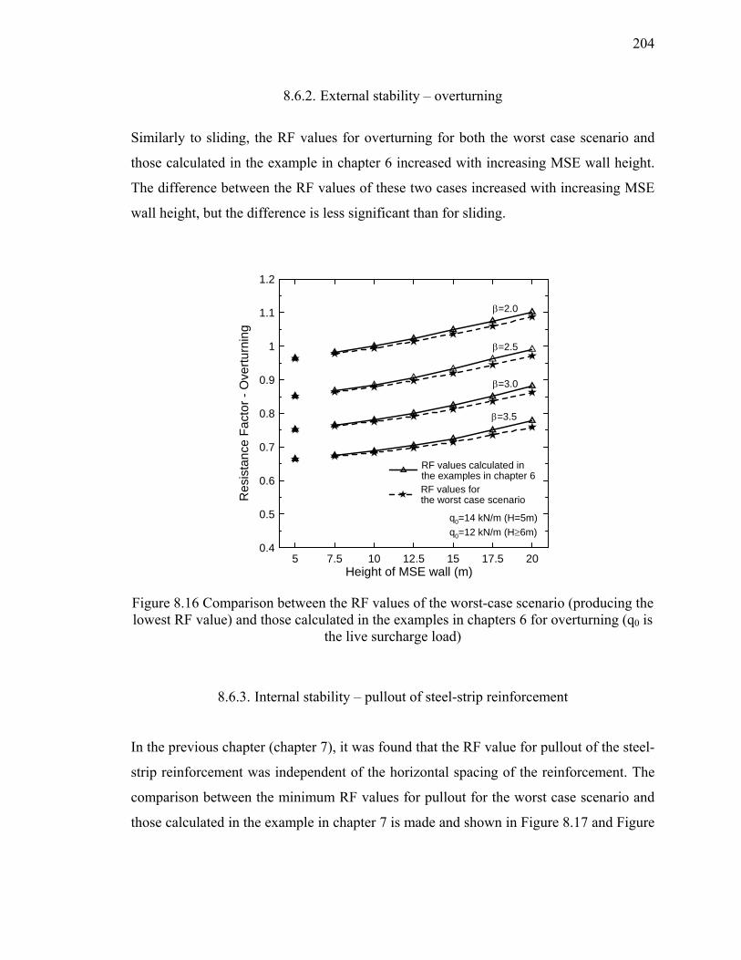
204
8.6.2. External stability – overturning
Similarly to sliding, the RF values for overturning for both the worst case scenario and
those calculated in the example in chapter 6 increased with increasing MSE wall height.
The difference between the RF values of these two cases increased with increasing MSE
wall height, but the difference is less significant than for sliding.
5 7.5 10 12.5 15 17.5 20Height of MSE wall (m)
0.4
0.5
0.6
0.7
0.8
0.9
1
1.1
1.2
Res
ista
nce
Fact
or -
Ove
rturn
ing
RF values calculated in the examples in chapter 6
q0=12 kN/m (H≥6m)q0=14 kN/m (H=5m)
RF values for the worst case scenario
β=2.0
β=2.5
β=3.0
β=3.5
Figure 8.16 Comparison between the RF values of the worst-case scenario (producing the lowest RF value) and those calculated in the examples in chapters 6 for overturning (q0 is
the live surcharge load)
8.6.3. Internal stability – pullout of steel-strip reinforcement
In the previous chapter (chapter 7), it was found that the RF value for pullout of the steel-
strip reinforcement was independent of the horizontal spacing of the reinforcement. The
comparison between the minimum RF values for pullout for the worst case scenario and
those calculated in the example in chapter 7 is made and shown in Figure 8.17 and Figure
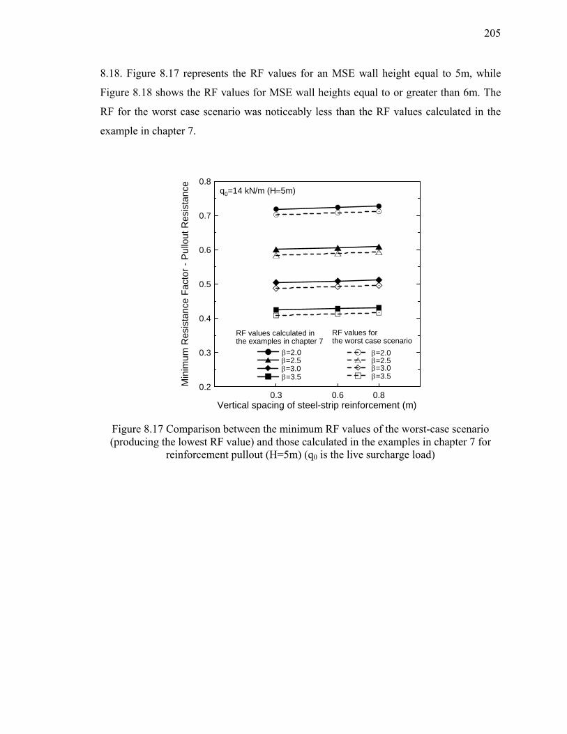
205
8.18. Figure 8.17 represents the RF values for an MSE wall height equal to 5m, while
Figure 8.18 shows the RF values for MSE wall heights equal to or greater than 6m. The
RF for the worst case scenario was noticeably less than the RF values calculated in the
example in chapter 7.
Vertical spacing of steel-strip reinforcement (m)
0.2
0.3
0.4
0.5
0.6
0.7
0.8M
inim
um R
esis
tanc
e Fa
ctor
- P
ullo
ut R
esis
tanc
e
β=2.0β=2.5β=3.0
q0=14 kN/m (H=5m)
0.3
β=2.0
0.6
β=2.5
0.8
β=3.0
RF values calculated in the examples in chapter 7
RF values forthe worst case scenario
β=3.5 β=3.5
Figure 8.17 Comparison between the minimum RF values of the worst-case scenario (producing the lowest RF value) and those calculated in the examples in chapter 7 for
reinforcement pullout (H=5m) (q0 is the live surcharge load)
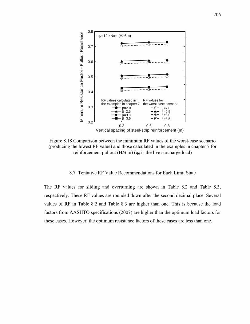
206
Vertical spacing of steel-strip reinforcement (m)
0.2
0.3
0.4
0.5
0.6
0.7
0.8
Min
imum
Res
ista
nce
Fact
or -
Pul
lout
Res
ista
nce
β=2.0β=2.5β=3.0
q0=12 kN/m (H≥6m)
0.3
β=2.0
0.6
β=2.5
0.8
β=3.0
RF values calculated inthe examples in chapter 7
RF values forthe worst case scenario
β=3.5 β=3.5
Figure 8.18 Comparison between the minimum RF values of the worst-case scenario (producing the lowest RF value) and those calculated in the examples in chapter 7 for
reinforcement pullout (H≥6m) (q0 is the live surcharge load)
8.7. Tentative RF Value Recommendations for Each Limit State
The RF values for sliding and overturning are shown in Table 8.2 and Table 8.3,
respectively. These RF values are rounded down after the second decimal place. Several
values of RF in Table 8.2 and Table 8.3 are higher than one. This is because the load
factors from AASHTO specifications (2007) are higher than the optimum load factors for
these cases. However, the optimum resistance factors of these cases are less than one.

207
Table 8.2 RF values for sliding criterion
Height of MSE wall(m)
Target reliability index βT
2.0 2.5 3.0 3.5
5 0.98 0.86 0.76 0.67
7.5 1.02 0.90 0.79 0.69
10 1.05 0.94 0.83 0.73
12.5 1.10 0.98 0.88 0.77
15 1.14 1.03 0.93 0.82
17.5 1.17 1.07 0.97 0.87
20 1.20 1.11 1.02 0.92
Table 8.3 RF values for overturning criterion
Height of MSE wall(m)
Target reliability index βT
2.0 2.5 3.0 3.5
5 0.96 0.85 0.75 0.66
7.5 0.98 0.86 0.76 0.67
10 0.99 0.88 0.78 0.68
12.5 1.01 0.90 0.79 0.69
15 1.04 0.92 0.81 0.71
17.5 1.06 0.94 0.84 0.73
20 1.09 0.97 0.86 0.75
The minimum pullout RF values from the values for all the steel-strip
reinforcement levels are given in Table 8.4 and Table 8.5. The small difference of RF
values between Table 8.4 and Table 8.5 results from different magnitudes of the live
uniform surcharge load acting on the top of the reinforced soil (14kN/m for 5m-high
MSE walls and 12 kN/m for MSE walls more than 6m tall). Typically, the reinforcement
length is controlled by the first reinforcement length, and the RF for pullout is proposed

208
accordingly. In addition, the RF values for structural failure of steel-strip reinforcement
are given in Table 8.6.
Table 8.4 Minimum RF value for pullout of steel-strip reinforcement for 5m-high MSE wall (with q0=14 kN/m)
The first reinforcementdepth (m)
Target reliability index βT
2.0 2.5 3.0 3.5
0.3 0.70 0.58 0.48 0.40
0.6 0.70 0.58 0.49 0.41
0.8 0.71 0.59 0.49 0.41
Table 8.5 Minimum RF value for pullout of steel-strip reinforcement for MSE walls more than 6m-tall (with q0=12 kN/m)
The first reinforcement depth (m)
Target reliability index βT
2.0 2.5 3.0 3.5
0.3 0.70 0.58 0.48 0.40
0.6 0.71 0.59 0.49 0.41
0.8 0.71 0.59 0.49 0.41
Table 8.6 RF value for structural failure of steel-strip reinforcement
Target reliability index, βT
3.5 3 2.5 2
RF 0.66 0.72 0.79 0.87

210
CHAPTER 9. CONCLUSIONS AND RECOMMENDATIONS
9.1. Introduction
The main objective of this project was to develop LRFD methods for slopes and MSE
walls using ULS design concepts and probability theory. The study also suggests
resistance factor (RF) values that are compatible with the LFs of the AASHTO LRFD
specifications (2007). The suggested optimum factors for LRFD of slopes and RF values
for LRFD of MSE walls were obtained from the result of extensive reliability analyses on
the basis of a rational assessment of uncertainties of the parameters that are used in the
analysis.
To accomplish these goals for LRFD of slopes, (1) the algorithm for LRFD of
slopes was developed, (2) the sources of uncertainty of each pertinent property were
classified and examined, (3) the Gaussian random field concept was used for a more
realistic representation of the soil parameters of slopes, (4) extensive Monte Carlo
simulations were conducted to find the driving and resisting moments at the ULS for
which the calculated probability of failure is equal to the target probability of failure, (5)
optimum load and resistance factors were obtained using the ultimate limit state values
and nominal values of driving and resisting moments.
For LRFD of MSE walls, (1) Limit states were identified, (2) a framework for
LRFD of MSE walls was developed, (3) ULSs were mathematically defined in a way that
is consistent with both the physics of the problems and the engineering requirements, (4)
the uncertainties of parameters, transformations, and models used in the analysis were
assessed, (5) reliability analysis for each limit state was done using FORM, and (6) the
RF value for each limit state was suggested.

211
At the end of this chapter, recommendations are presented for implementation in
practice that could improve the accuracy and reliability of the RF values for LRFD of
slopes and MSE walls.
9.2. LRFD of Slopes
We have successfully employed Gaussian random field theory for the representation of
spatial (inherent) soil variability. The reliability analysis program developed for LRFD of
slopes using Monte Carlo simulations in conjunction with the soil parameters represented
by Gaussian random fields works well and provides reliable results.
Even for the given target probability of failure, geometry of slope, and mean
values of parameters and their uncertainties, there is no uniqueness of the RF value for
slopes. In other words, the RF value resulting from Monte Carlo simulations varies from
case to case. This is because the Gaussian random fields and also the slip surface at the
ULS for each random realization of a slope defined by the mean values of the strength
parameters and unit weights of each layer and of the live load are different from
simulation to simulation. We have proposed a way to deal with this nonuniqueness that
provides an acceptable basis on which to make resistance factor recommendations.
9.3. LRFD of MSE Walls
For each limit state, the First-Order Reliability Method (FORM) was successfully used to
compute the values of loads and resistance at the ULS for the given target reliability
index and the corresponding optimal load and resistance factors.
A parametric study of the external stability (sliding and overturning) of MSE
walls identified the unit weight of the retained soil as the parameter with the most impact
on the RF value. This seems to be because the change of the unit weight of the retained
soil results in a change of the composition of the uncertainty of the total lateral load
acting on the reinforced soil. For example, if the unit weight of the retained soil increases,
212
the ratio of the lateral load due to the live uniform surcharge load to the lateral load due
to the self-weight of the retained soil decreases. Therefore, the uncertainty of the total
load decreases because the lateral load due to the live uniform surcharge load has a much
higher bias factor and COV compared to those of the lateral load due to the self-weight of
the retained soil. Consequently, the RF values for sliding and overturning increase as the
height of the MSE wall increases.
For pullout of the steel-strip reinforcement, the most important parameter on the
RF value is the relative density of the reinforced soil because not only the relative density
has the highest COV among all the parameters but also the mean value of the relative
density has a significant influence on the pullout resistance factor. In addition, the level
(or the vertical location) of the steel-strip reinforcement also has considerable impact on
the RF value because the reinforcement level changes the uncertainty of total load
significantly by changing the ratio of the load due to the self-weight of the reinforced soil
to the load due to the live uniform surcharge load.
In this report, we found the worst cases, which have the lowest RF values, by
varying the parameters within their possible ranges for different MSE wall heights and
different target reliability indices. The “worst-case” RF values for sliding and overturning
are given in the report (Table 8.2 and Table 8.3). The “worst-case” RF values for pullout,
which occur at the first reinforcement level from the top of the MSE wall, are suggested
as RF values to use in pullout failure checks (Table 8.4 and Table 8.5). The “worst-case”
RF values for structural failure are recommended as RF values to use in structural failure
checks (Table 8.6). Usually, the required reinforcement length L at the first reinforcement
level from the top of an MSE wall is used for all the other reinforcement levels when the
vertical and horizontal spacing of the reinforcements are the same. Therefore, in general,
this required reinforcement length L can be calculated using the RF value for pullout at
the first reinforcement depth z.

213
9.4. Recommendations for Future Study
RF values for LRFD of slopes and MSE walls in this report are calculated based
on analyses done for a limited number of conditions. The RF values for slopes and MSE
wall designs given in this report are valid only when designers use (i) the equations for
load and resistance and (ii) the test methods for design parameters given in this report.
The RF values are computed for two different target probabilities of failure (Pf = 0.001
and 0.01) for slopes and four different target reliability indices (βT=2.0, 2.5, 3.0, and 3.5)
for MSE walls. The higher values of target probability of failure (0.01) and the lower
values of target reliability index (2.0 and 2.5) are provided for illustration purposes, as
they would typically be excessively daring in most design problems. For slope stability,
resistance factors for a probability of failure lower than 0.001 would require considerable
time to calculate. In practice, the importance of the structure may vary; therefore,
designers should select an appropriate target probability of failure (or target reliability
index) that would produce an economical design without excessive risk to the stability of
a structural and geotechnical system.
For development of complete and reliable sets of resistance factors for LRFD of
slopes and MSE walls, we recommend the following:
(1) It is necessary to perform comprehensive research on the classification of the type
of error associated with measurements, which is a process that requires extensive
effort in testing and data collection. This effort would make it possible to assess
the uncertainty of systematic error more accurately. As uncertainties in
parameters reflect directly on RF values, improved assessment of these
uncertainties would be very beneficial.
(2) The load factors provided in the current AASHTO LRFD specifications (2007)
are equal to one regardless of the load type. This means that RF values (0.75
when the geotechnical parameters are well defined and the slope does not support
or contain a structural element, and 0.65 when the geotechnical parameters are
based on limited information or the slope contains or supports a structural

214
element) proposed in the specifications are inverse values of the factors of safety
(1.3 and 1.5) that were given in the old AASHTO specifications. Thus, LRFD of
slopes as currently covered by the AASHTO specifications is in effect the same as
Working Stress Design (WSD). Use of the algorithm provided in this report
would produce appropriate load factors that reflect the uncertainty of the
corresponding loadings and allow determination of suitable resistance factors.
Then, the current load and resistance factor for LRFD of slopes in the AASHTO
LRFD specifications could be updated to more closely reflect the principles of
LRFD.
(3) More analyses are necessary for determining RF values for slope design. The
following all should be explored: (i) different geometries; (ii) different external
loading conditions (load type, location, and magnitude); (iii) different
combinations of soil layers; (iv) different combinations of the values of soil
property (considering wide ranges of soil property values); (v) wider ranges of
probability of failure (and, in particular, lower probabilities of failure); (vi)
repeatability checks to further validate the method proposed to handle the
nonuniqueness of resistance and load factors resulting from different simulations.
(4) Similarly to slopes, more analyses varying MSE wall geometry, loading condition
and soil properties will be helpful to expand LRFD for MSE wall design for
different site conditions.
(5) The RF value for general loss of stability of MSE walls could be examined using
the appropriate load factors determined from extensive Monte Carlo simulations
for LRFD of slopes.
(6) For certain geotechnical structures, such as levees, dams or abutments of large
and massive bridges, lower target probabilities of failure (or higher target

215
reliability index) should be considered. A more careful study of acceptable values
of probability of failure should be conducted.

216
LIST OF REFERENCES
AASHTO, 2002, Standard Specifications for Highway Bridges, American Association of
State Highway and Transportation Officials, 17th Edition, Washington, D.C., USA
AASHTO, 2007, LRFD Bridge Design Specifications, American Association of State
Highway and Transportation Officials, 4th Edition, Washington, D.C., USA
AISC, 2005, Specification for Structural Steel Buildings, American Institute of Steel
Construction, Inc, 3rd printing, Chicago, Illinois, USA
ASCE/SEI 7-05, 2006, Minimum Design Loads for Buildings and Other Structures,
American Society of Civil Engineers
Al-Homoud, A.S. And Tanash, N. (2001). “Monitoring and analysis of settlement and
stability of an embankment dam constructed in stages on soft ground.” Bulletin of
Engineering Geology and the Environment, 59(4), 259-284.
Allen, T., Christopher, B., Elias, V., and DeMaggio, J. (2001). Development of the
Simplified Method for Internal Stability Design of Mechanically Stabilized Walls,
WDOT, Report number WA-RD 513.1
Allen, T. and Bathurst, R. J. (2003). Prediction of Reinforcement Loads in Reinforced
Soil Walls, WDOT, Report number WA-RD 522.2
217
Asaoka, A. and A-Grivas, D. (1982). “Spatial Variability of the Undrained Strength of
Clays.” Journal of Geotechnical Engineering Division, 108(GT5), 743-756.
Auvinet, G. and Gonzalez, J.L. (2000). “Three-Dimensional Reliability Analysis of Earth
Slopes.” Computers and Geotechnics, 26, 247-261.
Baecher, G.B. (1982). “Simplified Geotechnical Data Analysis.” Proceedings of the
NATO Advanced Study Institute on Reliability Theory and its Application in Structural
and Soil Mechanics, Bornholm, Denmark, Martinus Nijhoff, 257-277.
Becker, D.E. (1996). “Eighteenth Canadian Geotechnical Colloquium: Limit States
Design for Foundations. Part I. An Overview of the Foundation Design Process.”
Canadian Geotechnical Journal, 33, 956-983.
Becker, D.E. (1996). “Eighteenth Canadian Geotechnical Colloquium: Limit States
Design for Foundations. Part II. Development for the National Building Code of
Canada.” Canadian Geotechnical Journal, 33, 984-1007.
Bishop, A.W (1948). “Some factors Involved in the Design of a large Earth Dam in the
Thames Valley,” Proc. 2nd International Conference on Soil Mechanics and Foundation
Engineering, Rotterdam, Paper 4, 13-18.
Bishop, A.W. (1955). ‘‘The use of the slip circle in the stability analysis of slopes.’’
Geotechnique, 5, 7–17.
Broms, B.B. and Ingleson, I. (1971). ‘‘Earth Pressure against the Abutments of a Rigid
Frame Bridge.’’ Geotechnique, 21(1), 15–28.
Carder, D.R., Pocock, R.G., and Murray, R.T. (1977). ‘‘Experimental Retaining Wall
Facility-Lateral Stress Measurements with Sand Backfill.’’ Rep. 766, Transport and Road
Research Laboratory, Crowthorne, Berkshire, England.

218
Chaisson, P., Lafleur, J., Soulie, M. and Law, K.T. (1995). “Characterizing Spatial
Variability of a Clay by Geostatistics”, Canadian Geotechnical Journal, No.32, 1-10.
Chen, Y. (1999). “Practical Analysis and Design of MSE Walls by LRFD Method.” J.
Engineering Technology, Spring, 8-17.
Chen, Y. (2000). “Practical analysis and design of mechanically-stabilized earth walls - I.
Design philosophies and procedures.” Engineering Structures, 22, 793-808.
Chen, Y. (2000). “Practical analysis and design of mechanically-stabilized earth walls –
II. Design comparisons and impact of LRFD method.” Engineering Structures, 22, 809-
830.
Cherubini, C. (1997). “Data and Considerations on the Variability of Geotechnical
Properties of Soils.” Proceedings of the International Conference on Safety and
Reliability, ESREL97, Lisbon. Vol. 2. 1583-1591.
Cherubini, C. (2000) Reliability evaluation of shallow foundation bearing capacity in c′-
φ′ soils. Canadian Geotechnical Journal. 37, 264–269.
Chowdhury, R.N. (1984). “Recent Developments in Landslide Studies: Probabilistic
Methods.” Fourth International Symposium on Landslides, Toronto. 209-228.
Chowdhury, R. and Flentje, P.N. (2002). “Uncertainties in Rainfall-induced Landslide
Hazard.” Quarterly Journal of Engineering Geology and Hydrogeology, 35, 61-70.
Christian, J.T., Ladd, C.C., and Baecher, G.B. (1994). “Reliability applied to slope
stability analysis.” Journal of Geotechnical Engineering Division, 120(12), 2180-2207.

219
Corte, J. (1977). “La Methode des Elements Finis Appliqué an Ouvrages en Terre
Armee,” Buill. de Liais, LCPC, 90, 37-47.
Das, B.M. (1995). Principles of Geotechnical Engineering, PWS Engineering, Boston.
DeGroot, D.J. and Baecher, G.B. (1993). “Estimating Autocovariances of In-Situ Soil
Properties.” Journal of Geotechnical Engineering Division, 119(1), 147-166.
ECS (1994). Eurocode 7:Geotechnical Design-Part I: General Rules. European
Committee for Standardization, Central Secretariat, Brussels.
Ellingwood, B., Galambos, T.V., MacGregor, J.G. and Cornell, C.A. (1980).
Development of a probability based load criterion for American National Standard A58 -
Building Code Requirements for Minimum Design Loads in Buildings and other
Structures. National Bureau of Standards, Washington, D.C..
Ellingwood, B.R. (1999). “Wind Load Statistics for Probability-Based Structural
Design.” Journal of Structural Engineering, ASCE. 125(4), 453-463.
Fang, Y.S., Chen, J.M. and Chen, C.Y. (1997). “Earth pressures with sloping backfill,”
Journal of Geotechnical and Geoenvironmental Engineeeinrg, 123(3), 250-259.
Fenton, G.A. (1990). Simulation and Analysis of Random Fields, Ph.D. Thesis, Princeton
University, Princeton, New Jersey.
Foye, K. (2004) Limit States Design of Foundatin, JTRP final report, FHWA/IN/JTRP-
2004/21, Purdue University.

220
Foye, K. (2004). A Rational, Probabilistic Method for the Development of Geotechnical
Load and Resistance Factor Design. Ph.D thesis, Purdue University, West Lafayette,
Indiana.
Foye, K., Scott, B. and Salgado, R. (2006). "Assessment of Variable Uncertainties for
Reliability-Based Design of Foundations." Journal of Geotechnical and
Geoenvironmental Engineering, ASCE, 132(9), 1197-1207.
Foye, K., Scott, B. and Salgado, R. (2006). "Resistance Factors for Use in Shallow
Foundation LRFD." Journal of Geotechnical and Geoenvironmental Engineering, ASCE,
132(9), 1208-1218.
Fredlund, D.G. and Dahlman, A.E. (1972). “Statistical Geotechnical Properties of Glacial
Lake Edmonton Sediments.” First International Conference on Applications of Statistics
and Probability to Soil and Structural Engineering, Hong Kong, 203-228.
Goble, G. (1999). “Geotechnical Related Development and Implementation of Load and
Resistance Factor Design (LRFD) Methods”, NCHRP Synthesis 276, Transportation
Research Board, National Research Council, p. 68.
Hammitt, G.M. (1966). “Statistical Analysis of Data from Comparative Laboratory Test
Program Sponsored by ACIL.” Vicksburg, MS, U.S. Army Waterways Experiment
Station.
Harr, M.E. (1987), “Reliability based design in civil engineering,” McGraw Hill, London,
New York.
Hasofer, A.M. and Lind, N.C. (1974). “Exact and Invariant Second-Moment Code
Format.” Journal of the Engineering Mechanics Division, ASCE. 100(1), 111- 121.
221
Hendron (1963) A Typical relationship between the coefficient of earth pressure at rest
and the initial void ratio, Ph.D thesis.
Ingold, T.S. (1982). Reinforced Earth, Thomas Telford Ltd., London.
Jaksa, M.B., Kaggwa, W.S., and Brooker, P.I. (2000). “Experimental evaluation of the
scale of fluctuation of a stiff clay,” Application of statistics and probability: Civil
Engineering reliability and risk analysis; Proceedings of the ICASP 8 Conference,
Sydney, New Scout, Vol. 1, 415-422.
Jaky, J. (1944). “The Coefficient of Earth Pressure at Rest,” Journal for Society of
Hungarian Architects and Engineers, Budapest, Hungry, Oct. 355-358.
Juran, I. (1977). “Dimensionment Interne des Ouvrages en Terre Armee”, Thesis for
Doctorate of engineering, Laboratoire Central des Pons et Chaussees, Paris.
Juran, I. and Schlosser, F. (1978). “Theoretical Analysis of Failure in Reinforced Earth
Structures,” Proceedings of ASCE Symposium on Earth Reinforcement, Pittsburgh, 528-
555.
Kulhawy, F.H., Roth M.J.S. and Grioriu, M.D. (1991). “Some Statistical Evaluations of
Geotechnical Properties.” Proceedings 6th International Conference on Applied Statistics
and Probability in Civil Engineering, (2), Mexico City, 705-712.
Kulhawy, F.H., Birgisson, B. and Grigoriu, M.D. (1992). “Reliability-Based Foundation
Design for Transmission Line Structures: Transformation Models for In-Situ Tests”,
Report EL-5507(4), Electric Power Research Institute, Palo Alto, p113.
Lacasse, S.M., and Ladd, C.C. (1973). Behaviour of Embankments on New Liskeard
Varved Clay. Report R73-44, Department of Civil Engineering, MIT, p270.
222
Lacroix, Y. and Horn, H.M. (1973). “Direct Determination and Indirect Evaluation of
Relative Density and Its Use on Earthwork Construction Projects,” Evaluation of Relative
Density and Its Role in Geotechnical Projects Involving Cohesionless Soils, A
Symposium Presented at the Seventy-Fifth Annual Meeting, American Society for
Testing and Materials, LA.
Loehr, J.E., Finley, C.A. and Huaco, D. (2005). Procedures for Design of Earth Slopes
using LRFD, Report No. OR 06-010, University of Missouri-Columbia and Missouri
Department of Transportation, p80.
Low, B.K. and Tang, W.H. (1997). “Reliability Analysis of Reinforced Embankments on
Soft Ground,” Canadian Geotechnical Journal, 34(5), 672-685.
Luckman, P.G. (1987). Slope Stability Assessment under Uncertainty: A First-Order
Stochastic Approach. Ph.D. thesis, UC. Berkeley.
Mitchell, J.K. and Villet, W.C.B. (1987). Reinforcement of Earth Slopes and
Embankments, NCHRP Report 290, Transportation Research Board, Washington, DC.,
323pp.
Muszynski, M.R. (2006). “Determination of Maximum and Minimum Densities of Poorly
Graded Sands Using a Simplified Method,” Geotechnical Testing Journal, 29(3), 1-10.
Negussey, D, Wijewickreme, W.K.D. and Vaid, Y.P. (1987). “Constant-volume friction
angle of granular materials,” Canadian Geotechnical Journal, 25, 50-55.
Nowak, A.S. (1994). "Load Model for Bridge Design Code." Canadian Journal of Civil
Engineering. 21, 36-49.
223
Okochi, Y. and Tatsuoka, F. (1984). “Some factors affecting K0-values of sand measured
in triaxial cell,” Soils and Foundations, 24(3), 52-68.
Orchant, C.J., Kulhawy, F.H., and Trautmann, C.H. (1988). Critical Evaluation of In-Situ
Test Methods and their Variability. Report EL-5507, Vol. 2, Electric Power Research
Institute, Palo Alto.
Paikowsky, Samuel G. (2004). Load and Resistance Factor Design for Deep
Foundations. NCHRP Report 507. Washington, D.C.: Transportation Research Board.
Phoon, K.K. and Kulhawy, F.H. (1999). “Characterization of Geotechnical Variability.”
Canadian Geotechnical Journal, 36(4), 612-624.
Poulos, S.J. and Hed, A. (1973). “Density Measurements in a Hydraulic Fill,” Evaluation
of Relative Density and Its Role in Geotechnical Projects Involving Cohesionless Soils,
A Symposium Presented at the Seventy-Fifth Annual Meeting, American Society for
Testing and Materials, LA.
Popescu, R., Prevost, J.H. and Deodatis, G. (2005), “3D effects in seismic liquefaction of
stochastically variable soil deposits,” Geotechnique, Vol. 55, No. 1, pp. 21-31.
Pradhan, T.B.S., Tatsuoka, F. and Horii, N. (1988). “Strength and Deformation
Characteristics of Sand in Torsional Simple Shear,” Soils and Foundations, 28(3), 131-
148.
Rackwitz, R. (2000). “Reviewing Probabilistic Soils Modelling.” Computers and
Geotechnics, 26, 199-223.
Salgado, R. (2008). The Engineering of Foundations. McGraw-Hill.

224
Santamarina, J., Altschaeffl, A., and Chameau, J. (1992). Reliability of Slopes:
Incorporating Qualitative Information. Transportation Research Record 1343, 1-5.
Schlosser, F. (1978). “La Terre Armee, Historique Development Actuel et Futur,” Proc.
Symp. Soil Reinforcing and Stabilising Techq., NSWIT/NSW Univ., 5-28.
Schlosser, F. and Elias, V. (1978). “Friction in Reinforced Earth,” Proceedings ASCE
Symposium on Earth Reinforcement, Pittsburgh, 735-762.
Schlosser, F. and Segrestin, P. (1979). “Local Stability Analysis Method of Design of
Reinforced Earth Structures,” Proceedings of International Conference on Soil
Reinforcement, 1, 157-162.
Scott, B. (2002). Development of Load and Resistance Factor Design Method for
Shallow Foundations. Ph.D. Thesis. Purdue University. West Lafayette, Indiana.
Sherif, M.A., Fang, Y.S., and Sherif, R.I. (1984). “KA and K0 behind Rotating and Non-
Yielding walls.” Journal of Geotechnical Engineering Division, 110, 41-56.
Simpson, B. (1992). “Partial factors of safety for design of retaining walls.”
Geotechnique, 42, 131-136.
Soulie, M., Montes, P. and Silvestri, V. (1990). “Modelling Spatial Variability of Soil
Parameters.” Canadian Geotechnical Journal, 27(5), 617-630.
Spry, M.J., Kulhawy, F.H., and Grigoriu, M.D. (1988). A Probability-Based Geotechnical
Site Characterization Strategy for Transmission Line Structures. Report EL-5507, Vol. 1,
Electric Power Research Institute, Palo Alto.
Suzuki, M. and Takada, T. (1998). Discussion on “Response of Pile Embedded in
Stochastic Ground Media,” Structural Safety, 20, 189-193.

225
Tatsuoka, F. (1987). Discussion on “The Strength and Dilatancy of sands,”
Geotechnique, 37(2), 219-226.
Tippett, L.H.C. (1925). “On the Extreme Individuals and the Range of Samples Taken
from a Normal Population.” Biometrika. 17(3/4), 364-387.
Vanmarcke, E.H. (1977), “Probabilistic modeling of soil profiles,” Journal of
Geotechnical Engineering Division, 103(GT11), 1227-1246.
Vanmarcke, E.H. (1977). “Reliability of Earth Slopes”, Journal of Geotechnical
Engineering Division, 103(GT11), 1247 - 1265.
Vanmarcke, E.H. (1983). Random Fields: Analysis & Synthesis, MIT Press, Cambridge,
p383.
Verdugo, R. and Ishihara, K. (1996). “The steady state of sandy soils,” Soils and
Foundations, 36(2), 81-91.
Yang, H., White, D.J., Schaefer, V.R. (2005). Innovative Solutions for Slope Stability
Reinforcement and Characterization: Vol. II, Final report CTRE Project 03-127, Center
for Transportation Research and Education Iowa State University.
White, D.J., Schaefer, V.R., Yang, H., and Thompson, M.J., (2005). Innovative Solutions
for Slope Stability Reinforcement and Characterization: Vol. I, Final report CTRE
Project 03-127. Center for Transportation Research and Education Iowa State University.

226
Wolff, T.F.(1994). Evaluating the reliability of existing levees. Report of a research
project entitled: Reliability of existing levees, prepared for U.S. Army Engineer
Waterways Experiment Station Geotechnical Laboratory.
Wu, T.H. (1974). “Uncertainty, Safety, and Decision in Soil Engineering.” Journal of
Geotechnical Engineering Division, 100(3), 329-348.

227
Appendix A. Symbols of the Loads in Table 2.2
DD: downdrag DC: dead load of structural components and nonstructural attachment DW: dead load of wearing surfaces and utilities EH: horizontal earth pressure load EL: accumulated locked-in force effects resulting from the construction process, including the secondary forces from post-tensioning ES: earth surcharge load EV: vertical pressure from dead load of earth fill BR: vehicular braking force CE: vehicular centrifugal force CR: creep CT: vehicular collision force CV: vessel collision force EQ: earthquake FR: friction IC: ice load IM: vehicular dynamic load allowance LL: vehicular live load LS: live load surcharge PL: pedestrian live load SE: settlement SH: shrinkage TG: temperature gradient TU: uniform temperature WA: water load and stream pressure WL: wind on live load WS: wind load on structure

228
Appendix B. Theory of Probability, Basic Statistics, and Its Application using Monte Carlo Simulation and First-Order Reliability Method (FORM)
B.1. Probability Density Function and Cumulative Distribution Function
A Probability density function (PDF) represents a probability distribution of a
particular random variable x, such as a probability histogram. For the random variable x,
PDF px(x) of x is a nonnegative function and its integral from −∞ to +∞ is equal to one:
xp (x)dx 1∞
−∞=∫ (B.1)
A Cumulative distribution function (CDF) of x′, denoted as Px(x′), is an integral
of px(x) from −∞ to x′:
x '
x xP (x ') p (x)dx−∞
= ∫ (B.2)
B.2 Basic Statistics
B.2.1. Mean and standard deviation of a population
When a population (size = n) of a certain random variable x exists, the mean μx
and variance Vx of the population of x are:
n
ii 1
x
x
n=μ =∑
(B.3)
229
( )n
2i x
i 1x
xV
n=
− μ=
∑ (B.4)
The standard deviation σx of the population of x is the positive square root of its
variance and is a measure of intensity of scatter about its mean μx.
( )n
2i x
i 1x x
xV
n=
− μσ = =
∑
(B.5)
B.2.2. Sample mean and standard deviation (Estimation of mean and standard deviation
of population)
The estimation of mean and standard deviation of a population of a certain
property x is possible from a sample that consists of “n” measurements (x1, x2, ⋅⋅⋅ , xn) of
x. These estimated mean and standard deviation of the population are called the sample
mean and sample standard deviation, and are denoted by x and sx, respectively. The
expressions for the sample mean and sample standard deviation are:
n
ii 1
xx
n==∑
(B.6)
( )n
2i
i 1x
x xs
(n 1)=
−=
−
∑ (B.7)
B.2.3. Covariance
230
Covariance of random variable x and y is a measure of the strength of correlation
between x and y. Covariance has the positive sign when x and y are positively correlated
(vice versa). When x and y are highly correlated, the absolute value of the covariance is
large. If x and y are independent of each other, covariance is equal to zero. And the
covariance between two identical random variables is equal to the variance of the
variable. The covariance of x and y is:
( )( )x yCov(x, y) E x y⎡ ⎤= − μ − μ⎣ ⎦ (B.8)
For discrete random variables x and y (i=1, 2, ··· , n), the covariance can be
expressed as:
( )( )n
i x i yi 1
x yCov(x, y)
n=
− μ − μ=
∑ (B.9)
B.2.4. Correlation coefficient
Correlation coefficient ρ(x,y) of random variable x and y is equal to covariance
divided by the standard deviation of these two random variables:
x y
Cov(x, y)(x, y)ρ =σ σ
(B.10)
By this normalization, the strength of correlation between x and y can be expressed as a
dimensionless number that is independent of the units of x and y. The correlation
coefficient varies from -1 to 1. Correlation coefficient value is equal to 1 (-1), if x and y
have perfect positive (negative) linear relationship.
B.2.5. Mean and standard deviation of a linear combination

231
If a certain variable Y can be expressed as a sum of n random variables (X1, X2, ··,
Xn) multiplied by n corresponding numerical constants (a1, a2, ··, an), Y is:
n
i ii 1
Y a X=
= ∑ (B.11)
Mean of Y is
[ ] [ ] [ ] [ ]n
i i 1 1 2 2 n ni 1
1 1 2 2 n n
E Y E a X a E X a E X a E X
a a a
=
⎡ ⎤= = + + +⎢ ⎥⎣ ⎦
= μ + μ + + μ
∑ L
L
(B.12)
When X1, X2, ··· , Xn are independent, variance of Y is
[ ] [ ] [ ] [ ]n
2 2 2i i 1 1 2 2 n n
i 1
V Y V a X a V X a V X a V X=
⎡ ⎤= = + + +⎢ ⎥⎣ ⎦∑ L (B.13)
Therefore, standard deviation of Y (X1, X2, ··· , Xn are independent) is
1 2 n
2 2 2 2 2 2Y 1 X 2 X n XV[Y] a a aσ = = σ + σ + + σL (B.14)
B.3. Bias Factor
The mean (or expected) value of a continuous random variable x whose
probability distribution function is px(x) can be expressed as:
232
b
x XaE[x] x p (x)dxμ = = ∫ (B.15)
where a and b are the lower and upper bound values of the PDF, respectively.
The mean of discrete values of x whose discrete probability distribution is px(xi)
can be expressed as: n
x i X ii 1
E[x] x p (x )=
μ = = ⋅∑ (B.16)
where n is the number of x observations (or measurements).
As shown in Figure B.1, the nominal value may not be equal to the mean value.
In other words, the nominal value could be either greater than or less than the mean
value. The nominal value is considered as a deterministic value that does not have
uncertainty. For example, in the analysis using working stress design (WSD), we
calculate the nominal resistance of geotechnical structures using nominal values for each
parameter. To account for the relationship between the nominal value and the mean value,
the bias factor (the ratio of mean value to nominal value) is introduced:
x
nominal
bias factor x
μ= (B.17)
where μx and xnominal are the mean and nominal values of a variable x, respectively.
Given that the bias factor of a variable x is a known value, the mean value of x
can be directly calculated by multiplying the bias factor by the nominal value.

233
x
nominal value
mean value
Xp ( )x
x
nominal value
mean value
Xp ( )x
Figure B.1 Mean and nominal values of a certain parameter x
B.4. Uncertainty Calculations
B.4.1. Uncertainty of a parameter
The coefficient of variation (COV) is defined as the ratio of the (estimated)
standard deviation [Eq. (B.7)] to its (estimated) mean [Eq. (B.6)]:
xsCOVx
= (B.18)
The COV is a measure of how much data are scattered from the mean value and
is a good reference for estimating the uncertainties of parameters. When we use a
constant COV for different mean values in the analysis (which implies the COV is
independent of the mean), we are imposing that the standard deviation of the sample is
proportional to the mean. In reality, it is likely that data are more scattered about the
mean as the mean increases.

234
x
x −σ
x
x +σx line
v
v
Figure B.2 Data scatter for a constant COV with respect to mean value
B.4.2. Uncertainty of transformation
Suppose that we have scattered paired data expressed as (xi, yi), where i=1, 2, ⋅⋅⋅,
n, and that yi and xi are related. When we perform a regression on the data set, we are
able to obtain the best fitting function, y = f(x). This regression function is determined by
minimizing the summation of [yi − f(xi)]2. All data of (xi, yi) do not fit exactly to the
function y = f(x) so that there exists scatter along the function f(x). Given the values of yi
(observed data) and f(xi) (predicted values), we can define an error for each datum as wi =
yi −f(xi). Thus, the mean value and the standard deviation of errors can be obtained:
n
ii 1
ww
n==∑
(B.19)
( )
( )
n2
ii 1
w
w ws
n 1=
−=
−
∑ (B.20)
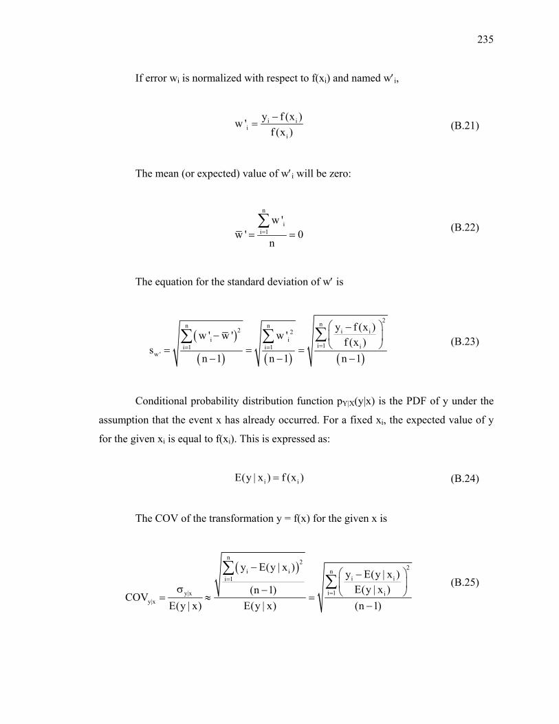
235
If error wi is normalized with respect to f(xi) and named w′i,
i ii
i
y f (x )w 'f (x )−
= (B.21)
The mean (or expected) value of w′i will be zero:
n
ii 1
w 'w ' 0
n== =∑
(B.22)
The equation for the standard deviation of w′ is
( )
( ) ( ) ( )
2nn n2 i i2
i ii 1 ii 1 i 1
w '
y f (x )w ' w ' w ' f (x )
sn 1 n 1 n 1
== =
⎛ ⎞−− ⎜ ⎟
⎝ ⎠= = =− − −
∑∑ ∑
(B.23)
Conditional probability distribution function pY|X(y|x) is the PDF of y under the
assumption that the event x has already occurred. For a fixed xi, the expected value of y
for the given xi is equal to f(xi). This is expressed as:
i iE(y | x ) f (x )= (B.24)
The COV of the transformation y = f(x) for the given x is
( )n
22ni i
i ii 1
i 1y|x iy|x
y E(y | x ) y E(y | x )E(y | x )(n 1)
COVE(y | x) E(y | x) (n 1)
=
=
− ⎛ ⎞−⎜ ⎟σ − ⎝ ⎠= ≈ =
−
∑∑
(B.25)
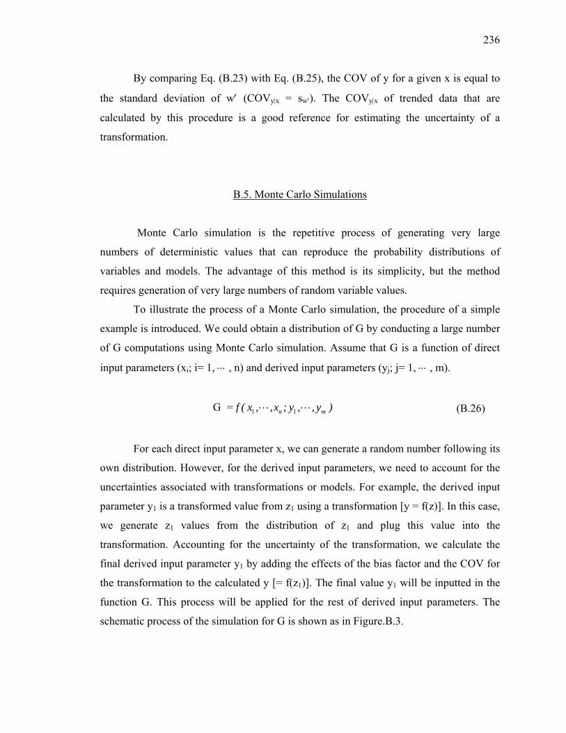
236
By comparing Eq. (B.23) with Eq. (B.25), the COV of y for a given x is equal to
the standard deviation of w′ (COVy|x = sw′). The COVy|x of trended data that are
calculated by this procedure is a good reference for estimating the uncertainty of a
transformation.
B.5. Monte Carlo Simulations
Monte Carlo simulation is the repetitive process of generating very large
numbers of deterministic values that can reproduce the probability distributions of
variables and models. The advantage of this method is its simplicity, but the method
requires generation of very large numbers of random variable values.
To illustrate the process of a Monte Carlo simulation, the procedure of a simple
example is introduced. We could obtain a distribution of G by conducting a large number
of G computations using Monte Carlo simulation. Assume that G is a function of direct
input parameters (xi; i= 1, ⋅⋅⋅ , n) and derived input parameters (yj; j= 1, ⋅⋅⋅ , m).
1 1G = n mf ( x , ,x ; y , , y )L L (B.26)
For each direct input parameter x, we can generate a random number following its
own distribution. However, for the derived input parameters, we need to account for the
uncertainties associated with transformations or models. For example, the derived input
parameter y1 is a transformed value from z1 using a transformation [y = f(z)]. In this case,
we generate z1 values from the distribution of z1 and plug this value into the
transformation. Accounting for the uncertainty of the transformation, we calculate the
final derived input parameter y1 by adding the effects of the bias factor and the COV for
the transformation to the calculated y [= f(z1)]. The final value y1 will be inputted in the
function G. This process will be applied for the rest of derived input parameters. The
schematic process of the simulation for G is shown as in Figure.B.3.
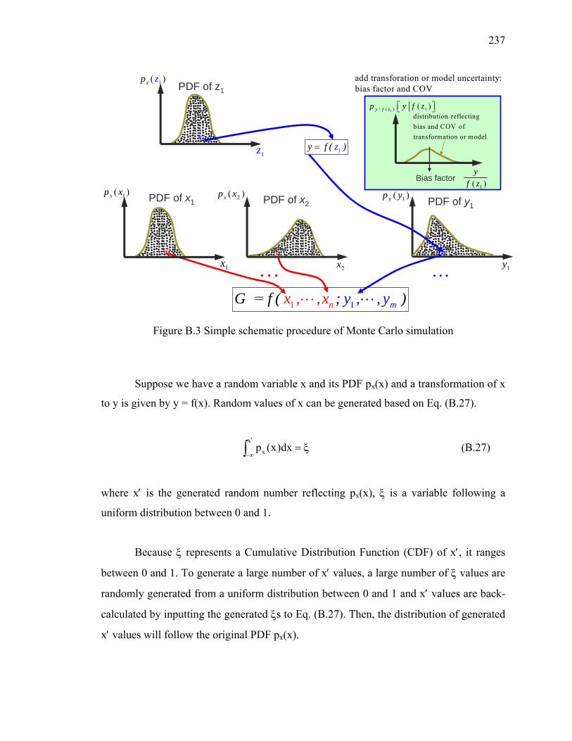
237
PDF of x11( )xp x
2x1x
11= mnx , ,x y ,G f ( ; ), yLL
L L1y
PDF of x22( )xp x
PDF of y11( )yp y
PDF of z11( )zp z
1z
add transforation or model uncertainty:bias factor and COV
1=y f ( z )
Bias factor
1/ ( ) 1( )⎡ ⎤⎣ ⎦y f zp y f z
1( )y
f z
distribution reflectingbias and COV of transformation or model
Figure B.3 Simple schematic procedure of Monte Carlo simulation
Suppose we have a random variable x and its PDF px(x) and a transformation of x
to y is given by y = f(x). Random values of x can be generated based on Eq. (B.27).
x
xp (x)dx′
−∞= ξ∫ (B.27)
where x′ is the generated random number reflecting px(x), ξ is a variable following a
uniform distribution between 0 and 1.
Because ξ represents a Cumulative Distribution Function (CDF) of x′, it ranges
between 0 and 1. To generate a large number of x′ values, a large number of ξ values are
randomly generated from a uniform distribution between 0 and 1 and x′ values are back-
calculated by inputting the generated ξs to Eq. (B.27). Then, the distribution of generated
x′ values will follow the original PDF px(x).

238
For each value of x′ from the large set generated as described, the prediction for
the corresponding y value is made using the transformation [ y f (x)= ], and the
uncertainty of this transformation is added to the predicted y value. By repeating this
process for all the generated x' values, we obtain the PDF of y, which is denoted by py(y)
in Figure B.3.
Compared to numerical integration, Monte Carlo simulation is much easier when
there are many variables and transformations to be considered in the analysis.
B.6. First-Order Reliability Method (FORM)
The concept of the reliability index β was introduced by Cornell (1969) and
Hasofer and Lind (1974). To apply the reliability index concept to limit state analysis, we
need to have a well defined limit state equation, a mean (or expected) value, a bias factor,
and a standard deviation (or COV) for each random variable used in the analysis.
For the case in which we have n random variables in the ultimate limit state
(ULS) equation, we can locate the failure surface from the ULS equation and the point
whose coordinates are the mean values of the n random variables in the n-dimension
imaginary space. Geometrically, the reliability index β is the ratio of the closest distance
between the point defined by the mean values of the n variables and the failure surface to
the standard deviation of the multiple probability density function for the n variables.
For example, when we have two variables (x and y) in the ULS equation, we
could draw both the point (μx, μy) defined by two mean values of the variables and the
failure surface defined by ULS equation (Figure B.4). It is possible to find the closest
distance between (μx, μy) and the failure surface from the figure and calculate the
standard deviation of multiple probability density function by assessing the uncertainties
associated with load and resistance. Then, the reliability index β is the ratio of the closest
distance to the standard deviation of the multiple probability density function.
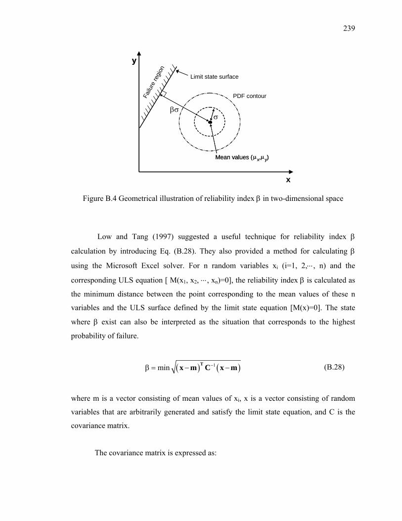
239
Mean values (μx,μy)
Limit state surface
Failu
re re
gion
y
PDF contour
Mean values (μx,μy)
x
y
σβσ
Figure B.4 Geometrical illustration of reliability index β in two-dimensional space
Low and Tang (1997) suggested a useful technique for reliability index β
calculation by introducing Eq. (B.28). They also provided a method for calculating β
using the Microsoft Excel solver. For n random variables xi (i=1, 2,⋅⋅⋅, n) and the
corresponding ULS equation [ M(x1, x2, ⋅⋅⋅, xn)=0], the reliability index β is calculated as
the minimum distance between the point corresponding to the mean values of these n
variables and the ULS surface defined by the limit state equation [M(x)=0]. The state
where β exist can also be interpreted as the situation that corresponds to the highest
probability of failure.
( ) ( )1min −β = − −Tx m C x m (B.28)
where m is a vector consisting of mean values of xi, x is a vector consisting of random
variables that are arbitrarily generated and satisfy the limit state equation, and C is the
covariance matrix.
The covariance matrix is expressed as:

240
( ) ( ) ( )( ) ( ) ( )
( ) ( ) ( )
1 1 1 2 1 n
2 1 2 2 2 n
n 1 n 2 n n
Cov x , x Cov x , x Cov x , xCov x , x Cov x , x Cov x , x
Cov x , x Cov x , x Cov x , x
⎡ ⎤⎢ ⎥⎢ ⎥=⎢ ⎥⎢ ⎥⎢ ⎥⎣ ⎦
C
L
L
M M O M
L
(B.29)
where Cov(xi, xj) is called the covariance between xi and xj.
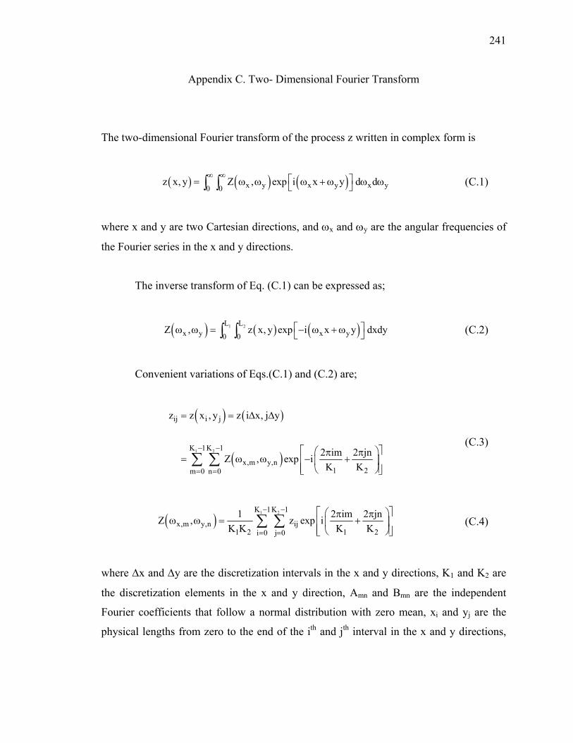
241
Appendix C. Two- Dimensional Fourier Transform
The two-dimensional Fourier transform of the process z written in complex form is
( ) ( ) ( )x y x y x y0 0z x, y Z , exp i x y d d
∞ ∞ ⎡ ⎤= ω ω ω + ω ω ω⎣ ⎦∫ ∫ (C.1)
where x and y are two Cartesian directions, and ωx and ωy are the angular frequencies of
the Fourier series in the x and y directions.
The inverse transform of Eq. (C.1) can be expressed as;
( ) ( ) ( )1 2L Lx y x y0 0
Z , z x, y exp i x y dxdy⎡ ⎤ω ω = − ω + ω⎣ ⎦∫ ∫ (C.2)
Convenient variations of Eqs.(C.1) and (C.2) are;
( ) ( )
( )1 2
ij i j
K 1K 1
x,m y,n1 2m 0 n 0
z z x , y z i x, j y
2 im 2 jnZ , exp iK K
− −
= =
= = Δ Δ
⎡ ⎤⎛ ⎞π π= ω ω − +⎢ ⎥⎜ ⎟
⎢ ⎥⎝ ⎠⎣ ⎦∑ ∑
(C.3)
( )1 2K 1K 1
x,m y,n ij1 2 1 2i 0 j 0
1 2 im 2 jnZ , z exp iK K K K
− −
= =
⎡ ⎤⎛ ⎞π πω ω = +⎢ ⎥⎜ ⎟
⎢ ⎥⎝ ⎠⎣ ⎦∑ ∑ (C.4)
where Δx and Δy are the discretization intervals in the x and y directions, K1 and K2 are
the discretization elements in the x and y direction, Amn and Bmn are the independent
Fourier coefficients that follow a normal distribution with zero mean, xi and yj are the
physical lengths from zero to the end of the ith and jth interval in the x and y directions,

242
and ωx,m (=2mπ/K1Δx) and ωy,n (=2nπ/K2Δy) are the angular frequencies of the Fourier
series in the x and y directions.
The complex exponential function in Eq. (C.3) and Eq. (C.4) can be expressed in
terms of sine and cosine by the Euler formula:
1 2 1 2 1 2
2 im 2 jn 2 im 2 jn 2 im 2 jnexp i cos isinK K K K K K
⎡ ⎤⎛ ⎞ ⎛ ⎞ ⎛ ⎞π π π π π π+ = + + +⎢ ⎥⎜ ⎟ ⎜ ⎟ ⎜ ⎟
⎢ ⎥⎝ ⎠ ⎝ ⎠ ⎝ ⎠⎣ ⎦ (C.5)
Assuming ( )x,m y,n mn mnZ , A iBω ω = + , then Eq. (C.3) and Eq. (C.4) can be written
as;
( )1 2K 1K 1
ij mn mn1 2 1 2m 0 n 0
2 im 2 jn 2 im 2 jnz A iB cos isinK K K K
− −
= =
⎡ ⎤⎛ ⎞ ⎛ ⎞π π π π= + + − +⎢ ⎥⎜ ⎟ ⎜ ⎟
⎢ ⎥⎝ ⎠ ⎝ ⎠⎣ ⎦∑ ∑ (C.6)
( )
1 2
x,m y,n
K 1K 1
mn mn ij1 2 1 2 1 2i 0 j 0
Z ,
1 2 im 2 jn 2 im 2 jnA iB z cos isinK K K K K K
− −
= =
ω ω
⎡ ⎤⎛ ⎞ ⎛ ⎞π π π π= + = + + +⎢ ⎥⎜ ⎟ ⎜ ⎟
⎢ ⎥⎝ ⎠ ⎝ ⎠⎣ ⎦∑ ∑
C.7)
By comparing the real part and imaginary part of each side of Eq. (C.6), Fourier
coefficients Amn and Bmn are
1 2K 1K 1
mn ij1 2 1 2i 0 j 0
1 2 im 2 jnA z cosK K K K
− −
= =
⎛ ⎞π π= +⎜ ⎟
⎝ ⎠∑ ∑ (C.8)
1 2K 1K 1
mn ij1 2 1 2i 0 j 0
1 2 im 2 jnB z sinK K K K
− −
= =
⎛ ⎞π π= +⎜ ⎟
⎝ ⎠∑ ∑
(C.9)

243
Because we are only considering the real part, zij can be represented as
1 2K 1K 1
ij mn mn1 2 1 2m 0 n 0
2 im 2 jn 2 im 2 jnz A cos B sinK K K K
− −
= =
⎛ ⎞⎛ ⎞ ⎛ ⎞π π π π= + + +⎜ ⎟⎜ ⎟ ⎜ ⎟⎜ ⎟⎝ ⎠ ⎝ ⎠⎝ ⎠
∑ ∑
(C.10)

244
Appendix D. Modified 6σ Method (Nσ Method)
Before introducing Nσ method, 6σ method is a technique that allows estimating the
standard deviation of a large numbers of data which show a normal distribution. Suppose
we have many data which have approximately a normally distribution. The assumption is
that these large numbers of data lie within the range of six standard deviations. The range
of data can be calculated by subtracting the minimum value of the data from the
maximum of the date. The standard deviation can be evaluated as follow.
max(data) min(date)6
σ−= (D.1)
where σ is the standard deviation.
Nσ method, which is called modified 6σ method, is devised by Tippett (1925).
Instead of the number 6 in 6σ method, he suggested the equivalent values of number Nσ
that are applicable to the data which have a normal distribution. Nσ is dependent of
number of data points. Therefore we do not have a sufficient number of data to apply 6σ
method, the estimation of standard deviation is possible by range [max(data)- min(data)]
divided by Nσ values. Nσ values are listed in Table D.1.
max(data) min(date)−=
Nσ
σ (D.2)

245
Table D.1 Nσ values for n data points
n Nσ n Nσ 2 1.1284 17 3.5879 3 1.6926 18 3.6401 4 2.0588 19 3.6890 5 2.3260 20 3.7350 6 2.5344 50 4.4982 7 2.7044 100 5.0152 8 2.8472 200 5.4921 9 2.9700 300 5.7556 10 3.0775 400 5.9364 11 3.1729 500 6.0734 12 3.2585 600 6.1835 13 3.3360 700 6.2752 14 3.4068 800 6.3536 15 3.4718 900 6.4222 16 3.5320 1000 6.4829
0 200 400 600 800 1000Number of data
0
2
4
6
8
Nσ v
alue
Figure D.1 Plot of Nσ value versus number of data

246
Appendix E. Interface Friction Angle δp between Backfill Soil and Steel-Strip Reinforcement
Lings and Dietz tested three different sands [virgin Leighton Buzzard coarse sand (VLB),
medium Golden sand (MGS), and silver fine sand (SFS)] using special direct shear
apparatus to find the average interface friction angle for sand-sand and sand-steel
interfaces. For our analysis, SFS was not considered because fine sand is not a suitable
backfill material of the reinforced soil. The soil properties of two sands are shown in
Table E.1.
Table E.1 Soil properties of two sands
Sand Gs emin emax D10
(mm)
D50
(mm)
D60
(mm)
Uc Note
VLB 2.651 0.506 0.802 0.64 0.78 0.81 1.27 rounded
MGS 2.567 0.494 0.806 0.34 0.44 0.45 1.32 subrounded
From the result of tests (Table E.2), it was found that the interface friction angle is
a function of relative (or normalized) roughness Rn, relative density DR, vertical stress σ′v
and critical-state friction angle δcv. The relative roughness Rn is defined as an average of
heights Ra of peaks to D50 (diameter corresponding to weight-percent of soil finer than
50%):
50
= an
RRD
(D.1)
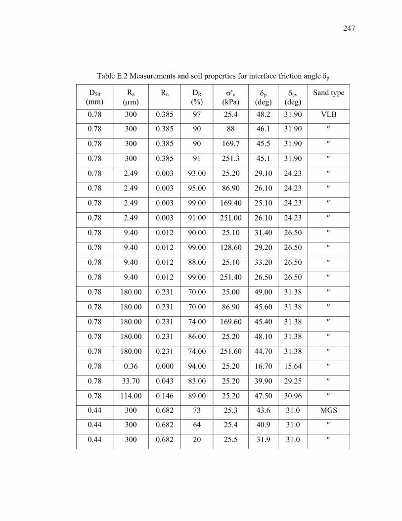
247
Table E.2 Measurements and soil properties for interface friction angle δp
D50 (mm)
Ra (μm)
Rn
DR (%)
σ'v (kPa)
δp (deg)
δcv (deg)
Sand type
0.78 300 0.385 97 25.4 48.2 31.90 VLB
0.78 300 0.385 90 88 46.1 31.90 ″
0.78 300 0.385 90 169.7 45.5 31.90 ″
0.78 300 0.385 91 251.3 45.1 31.90 ″
0.78 2.49 0.003 93.00 25.20 29.10 24.23 ″
0.78 2.49 0.003 95.00 86.90 26.10 24.23 ″
0.78 2.49 0.003 99.00 169.40 25.10 24.23 ″
0.78 2.49 0.003 91.00 251.00 26.10 24.23 ″
0.78 9.40 0.012 90.00 25.10 31.40 26.50 ″
0.78 9.40 0.012 99.00 128.60 29.20 26.50 ″
0.78 9.40 0.012 88.00 25.10 33.20 26.50 ″
0.78 9.40 0.012 99.00 251.40 26.50 26.50 ″
0.78 180.00 0.231 70.00 25.00 49.00 31.38 ″
0.78 180.00 0.231 70.00 86.90 45.60 31.38 ″
0.78 180.00 0.231 74.00 169.60 45.40 31.38 ″
0.78 180.00 0.231 86.00 25.20 48.10 31.38 ″
0.78 180.00 0.231 74.00 251.60 44.70 31.38 ″
0.78 0.36 0.000 94.00 25.20 16.70 15.64 ″
0.78 33.70 0.043 83.00 25.20 39.90 29.25 ″
0.78 114.00 0.146 89.00 25.20 47.50 30.96 ″
0.44 300 0.682 73 25.3 43.6 31.0 MGS
0.44 300 0.682 64 25.4 40.9 31.0 ″
0.44 300 0.682 20 25.5 31.9 31.0 ″

248
0.44 0.356 0.001 93 25.3 15.3 11.3 MGS
0.44 0.356 0.001 78 25.1 13.3 11.3 ″
0.44 0.356 0.001 69 25.2 11.5 11.3 ″
0.44 0.356 0.001 23 25.1 10.8 11.3 ″
0.44 2.49 0.006 94 25.1 27.7 24.2 ″
0.44 2.49 0.006 79 25.3 25.1 24.2 ″
0.44 2.49 0.006 69 25.3 25.10 24.2 ″
0.44 2.49 0.006 24 25.3 22.60 24.2 ″
0.44 9.40 0.021 93 25.2 39.00 27.5 ″
0.44 9.40 0.021 75 25.3 35.80 27.5 ″
0.44 9.40 0.021 68 25.4 33.40 27.5 ″
0.44 9.40 0.021 22 25.1 29.10 27.5 ″
0.44 33.7 0.077 92 25.3 47.10 31.0 ″
0.44 33.7 0.077 70 25.2 42.80 31.0 ″
0.44 33.7 0.077 26 25.3 33.70 31.0 ″
0.44 114.00 0.259 93 25.3 49.00 31.8 ″
0.44 114.00 0.259 78 25.3 43.40 31.8 ″
0.44 114.00 0.259 62 25.4 40.60 31.8 ″
0.44 114.00 0.259 27 25.2 33.90 31.8 ″
(VLS and MGS are two different soils explained in Table E.1, D50 is the diameter corresponding to weight-percent of soil finer than 50%, Ra is the average of heights of peaks, Rn is the relative roughness, DR is the relative density, σ′v is the vertical effective stress, δp is the interface friction angle, and δcv is the critical-state interface friction angle)
By performing multiple-variable regression (interface friction angle δp versus
relative roughness Rn, relative density DR, vertical effective stress σ′v, and critical-state
interface friction angle δcv) using the data provided in Lings and Dietz (2005), the
equation for interface friction angle δp can be expressed as:
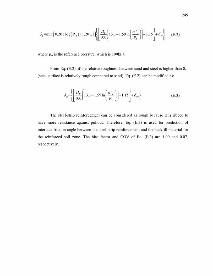
249
( )n'=min 0.201 log R +1.201,1 13.1 1.59ln 1.15
100vR
p cvA
DP
σδ δ⎧ ⎫⎡ ⎤⎛ ⎞⎛ ⎞⎪ ⎪− + +⎡ ⎤ ⎢ ⎥⎜ ⎟⎨ ⎬⎜ ⎟⎣ ⎦ ⎜ ⎟⎢ ⎥⎝ ⎠⎝ ⎠⎪ ⎪⎣ ⎦⎩ ⎭
(E.2)
where pA is the reference pressure, which is 100kPa.
From Eq. (E.2), if the relative roughness between sand and steel is higher than 0.1
(steel surface is relatively rough compared to sand), Eq. (E.2) can be modified as:
'= 13.1 1.59ln 1.15100
vRp cv
A
DP
σδ δ⎧ ⎫⎡ ⎤⎛ ⎞⎛ ⎞⎪ ⎪− + +⎢ ⎥⎜ ⎟⎨ ⎬⎜ ⎟⎜ ⎟⎢ ⎥⎝ ⎠⎝ ⎠⎪ ⎪⎣ ⎦⎩ ⎭
(E.3)
The steel-strip reinforcement can be considered as rough because it is ribbed to
have more resistance against pullout. Therefore, Eq. (E.3) is used for prediction of
interface friction angle between the steel-strip reinforcement and the backfill material for
the reinforced soil zone. The bias factor and COV of Eq. (E.3) are 1.00 and 0.07,
respectively.