Limit-Computable Mathematics and its

Applications

Susumu Hayashi & Yohji AkamaSep, 22, 2002

CSL’02, Edinburgh, Scotland, UK

LCM: Limit-Computable Mathematics

Constructive mathematics is a mathematics based on 0

1-functions, i.e. recursive functions.

In the same sense, LCM is a mathematics based on 0

2-functions.

The aim of the talk The talk aims to present basic theoretical ideas

of LCM and a little bit of the intended application as the motivation.

Thus, in this talk• THEORY

• APPLICATION (Proof Animation)

although the original project was application oriented and still the motto is kept.

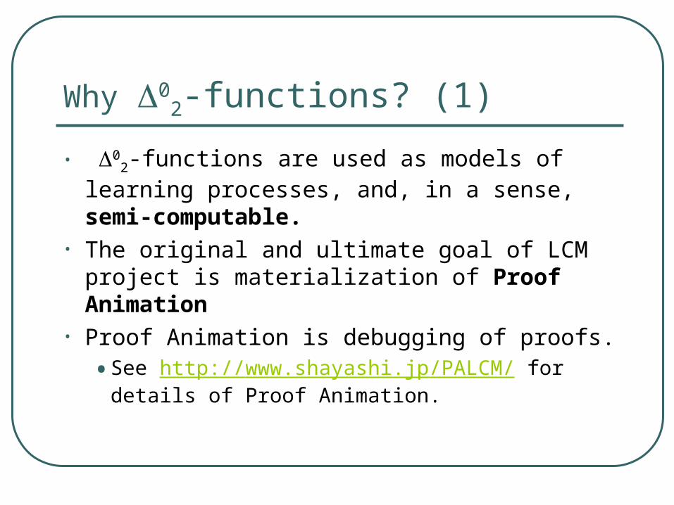
Why 02-functions? (1)

• 02-functions are used as models of learning

processes, and, in a sense, semi-computable.

• The original and ultimate goal of LCM project is materialization of Proof Animation

• Proof Animation is debugging of proofs.

• See http://www.shayashi.jp/PALCM/ for details of Proof Animation.

Why 02-functions? (2)

The 02-functions are expected to be useful

for Proof Animation as learning theoretic algorithms were useful in E. Shapiro’s Algorithmic Debugging of Prolog programs

Shapiro’s debugger debugged Prolog programs, i.e. axiom systems in Horn logic.

In a similar vein, an LCM proof animator is expected to debug axiom systems and proofs of LCM logic, which is at least a super set of predicate constructive logic.

An example of semi-computable learning process (1)

MNP (Minimal Number Principle):Let f be a function form Nat to Nat. Then, there is n : Nat such that f(n) is the smallest value among f(0), f(1), f(2),…

Nat : the set of natural numbers

An example of semi-computable learning process (2)

Such an n is not Turing-computable from f.

However, the number n is obtained in finite time from f by a mechanical “computation”.

A limit-computation of n (1)

Regard the function f as a stream f(0), f(1), f(2), …

Have a box of a natural number. We denote the content of the box by x.

A limit-computation of n (2)

Initialize the box by setting x=0. Compare f(x) with the next element of the

stream, say f(n). If the new one is smaller than f(x), then put n in the box. Otherwise, keep the old value in the box.

Repeat the last step forever.

A limit-computation of n (3)

The process does not stop. But your box will eventually contain the correct answer and after then the content x will never change.

In this sense, the non-terminating process “computes” the right answer in finite time.

You will have a right answer, but you will never know when you got it.

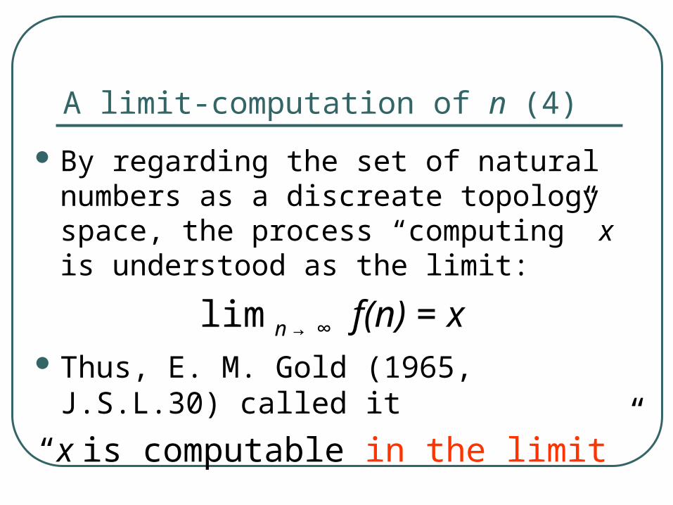
A limit-computation of n (4)

By regarding the set of natural numbers as a discreate topology space, the process “computing” x is understood as the limit:

lim n → ∞ f(n) = x Thus, E. M. Gold (1965, J.S.L.30) called it

“x is computable in the limit”

Limit computation as Learning process (1)

In computational learning theory initiated by Gold, the infinite series f(0), f(1), f(2),… is regarded as guesses of a learner to learn the limit value.

Limit computation as Learning process (2)

f is called a guessing function:

• The learner is allowed to change his mind. A guessing function represents a history of his mind changes.

When the learner stops mind changes in finite time, it succeeded to learn the right value. Otherwise, it failed to learn.

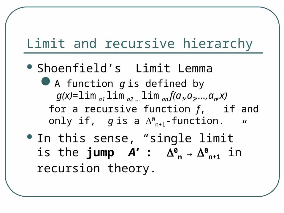
Limit and recursive hierarchy

Shoenfield’s Limit LemmaA function g is defined by

g(x)=lim a1 lim a2 ….lim an f(a1,a2,…,an,x)for a recursive function f, if and only if, g is a 0

n+1-function.

In this sense, “single limit” is the jump A’ : 0

n → 0n+1 in recursion theory.

Logic based on limit-computable functions (1)

As the 01-functions are the recursive

functions, 0n-functions may be

regarded as a generalized domain of computable functions.

For example, they satisfy axioms of some abstract recursion theory, e.g. BRFT by Strong & Wagner.

Logic based on limit-computable functions (2)

Semantics of constructive mathematics is given by realizability interpretations and type theories based on recursive functions.

Thus, when recursive functions are replaced by 0

n-functions, a new mathematics is created.

Logic based on limit-computable functions (3)

For n=2, it is a mathematics based on limit-computation or computational learning. It is LCM.

Note that limits in LCM are not nested. We may regard LCM is a mathematics

based on the single jump 0n → 0

n+1

Formal semantics of LCM (1)

Existing formal semantics of LCM are given by limit-function spaces and realizability interpretations or some interpretations similar.

The first and simplest one is Kleene realizability with limit partial functions with partial recursive guessing functions (Nakata & Hayashi)

Good Kripke or forcing style semantics and categorical semantics are longed for.

Formal semantics of LCM (2)

Learning theoretic limits must be extended to higher order functions to interpret logical implication and etcetras. Some extensions are necessary even for practical application reasons as well.

E.g. Nakata & Hayashi used “partial guessing functions”, which are rarely used in learning theory.

Formal semantics of LCM (3) Combinations of different approaches to

limit-functions plus different realizability interpretations (Kleene, modified, etc) make different semantics of LCM, e.g.,• Nakata & Hayashi already mentioned

• Akama & Hayashi: lim-CCC and modified realizability

• Berardi: A limit semantics based on limits over directed sets.

What kind of logic hold?

Logical axioms and rules of LCM depend on these semantics just as modified realizability and Kleene realizability define different constructive logics.

However, they have common characteristics:

semi-classical principles hold

0n- and 0

n-formulas

0n-and 0

n-formulas are defined as the usual prenex normal forms.

Thus, 03-formula is

Exists x.ForAll y.Exists z.A A definition not restricted to prenex form is

possible but omitted here for simplicity.

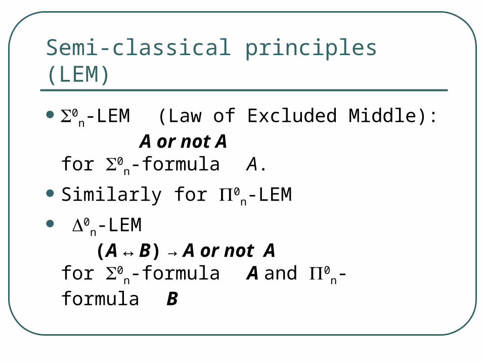
Semi-classical principles (LEM)

0n-LEM (Law of Excluded Middle):

A or not A 　for 0

n-formula A.

Similarly for 0n-LEM

0n-LEM

　 (A ↔ B) → A or not Afor 0

n-formula A and 0n-formula B

Semi-classical principles (DNE)

0n-DNE (Double Negation

Elimination): (not not A) → A for 0

n-formula A.

0n-DNE is defined similarly

Note: 01-DNE is Markov’s principle for

recursive predicates.

Some examples0

1-LEM ForAll x.A or not ForAll x.A

01-LEM

Exists x.A or not Exists x.A0

2-DNE not not Exists x.ForAll y.A → Exists x.ForAll y.A

03-LEM

Exists x.ForAll y.Exists z.A or not Exists x.ForAll y.Exists z.A

0n–DNE0

n–LEM

0n-1–LEM

0n–LEM

0n+1–DNE

0n–LEM

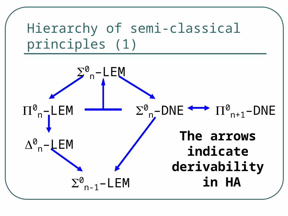
Hierarchy of semi-classical principles (1)

The arrows indicate

derivability in HA

Important Remark (1)

If we allow function parameters in recursive formulas, then the hierarchy collapses with the help of the full principle of function definition ForAll x.Exists!y.A(x,y) → Exists f.Forall x.A(x,f(x))

Because of the combination of these two iterate applications of limits.

Important Remark (2)

We keep the function definition principle and forbid function parameters in recursive predicates.

We may introduce function parameters for recursive functions.

LCM semi-classical principles

In all of the known semantics of LCM, the followings hold: 0

1-LEM, 01-LEM, 0

1-DNE, 02-DNE

In some semantics the followings also hold: 0

2-LEM, 02-DNE

These are LCM-principles since interpretable by single limits. The principles beyond these need iterated limits, and so non-LCM.

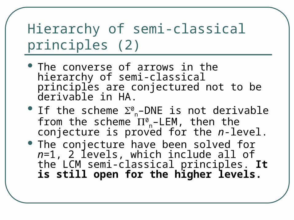
Hierarchy of semi-classical principles (2) The converse of arrows in the hierarchy of

semi-classical principles are conjectured not to be derivable in HA.

If the scheme 0n–DNE is not derivable from

the scheme 0n–LEM, then the conjecture is

proved for the n-level. The conjecture have been solved for n=1, 2

levels, which include all of the LCM semi-classical principles. It is still open for the higher levels.

What theorems are provable in LCM? (1)

Transfers from Reverse Mathematics:• If sets are identified with {0,1}-valued

function, almost all theorems proved in systems of Reverse Mathematics can be transferred into LCM.

Since Reverse Math. covers large parts of mathematics, we can prove very many classical theorems in LCM almost automatically thanks to e.g. Simpson’s book.

A recent development in LCM

01–LEM is the weakest LCM semi-

classical principle considered. Even below it, there is an interesting

semi-classical principle and corresponding theorems.

It’s Weak Koenig Lemma (WKL): “any binary branching tree with infinite nodes has an infinite path”.

WKL and LLPO

Bishop’s LLPO: not not (A or B) → A or B for A, B: 0

1-formulas WKL is constructively equivalent to

LLPO plus the bounded countable choice for 0

1-formulas.

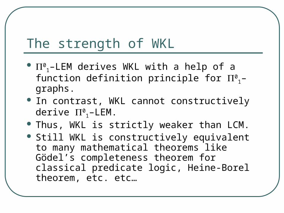
The strength of WKL

01–LEM derives WKL with a help of a

function definition principle for 01–graphs.

In contrast, WKL cannot constructively derive 0

1–LEM. Thus, WKL is strictly weaker than LCM. Still WKL is constructively equivalent to many

mathematical theorems like Gödel’s completeness theorem for classical predicate logic, Heine-Borel theorem, etc. etc…

Three underivability proofs

The underivability of 01-LEM is proved

by three different proofs:

• monotone functional interpretation (Kohlenbach)

• Standard realizability plus low degree model of WKL0 (Berardi, Hayashi, Yamazaki)

• Lifschitz realizability (Hayashi)

Open problem WKL seems to represent a class of non-

deterministic or multi-valued computation. Monotone functional interpretation and Lifschitz realizability and seem to give their models.

On the other hand, Hayashi’s proof uses Jockush-Soare’s the low degree theorem and the usual realizability, i.e., usual computation.

The relationship between these two groups of proofs would be a relationship of forcing and generic construction.

Open problem: Find out exact relationship.

Collaborators

The results on hierarchy and calibration are obtained in our joint works with the following collaborators: S. Berardi, H. Ishihara, U.Kohlenbach, T. Yamazaki, M. Yasugi