University of British ColumbiaCPSC 314 Computer Graphics

Jan-Apr 2007

Tamara Munzner

http://www.ugrad.cs.ubc.ca/~cs314/Vjan2007

Lighting/Shading I

Week 6, Wed Feb 14

2

News

• Homework 2 out today

• Project 2 out Friday• due Mon Feb 26 instead of Fri Feb 23

3

Reading for Today & Next 2 Lectures

• FCG Chap 9 Surface Shading

• RB Chap Lighting

4

Review: Scan Conversion

• convert continuous rendering primitives intodiscrete fragments/pixels• given vertices in DCS, fill in the pixels

• display coordinates required to provide scale fordiscretization

5

Correction: Making It Fast: ReuseComputation

• midpoint: if f(x+1, y+.5) < 0 then y = y+1

• on previous step evaluated f(x-1, y-.5) or f(x-1, y+.5)

• f(x+1, y) = f(x,y) + (y0-y1)

• f(x+1, y+1) = f(x,y) + (y0- y1) + (x1- x0)y=y0d = f(x0+1, y0+.5)for (x=x0; x <= x1; x++) {draw(x,y);if (d<0) then {y = y + 1;d = d + (x1 - x0) + (y0 - y1)

} else {d = d + (y0 - y1)

}

6

Review/Correction: Midpoint Algorithm• we're moving horizontally along x direction (first octant)

• only two choices: draw at current y value, or move up verticallyto y+1?

• check if midpoint between two possible pixel centers above orbelow line

• candidates• top pixel: (x+1,y+1)• bottom pixel: (x+1, y)

• midpoint: (x+1, y+.5)

• check if midpoint above or below line• below: pick top pixel• above: pick bottom pixel

• key idea behind Bresenham• reuse computation from previous step• integer arithmetic by doubling values

above: bottom pixel

below: top pixel

7

Review: Triangulating Polygons

• simple convex polygons• trivial to break into triangles• pick one vertex, draw lines to all others

not immediately adjacent• OpenGL supports automatically

• glBegin(GL_POLYGON) ... glEnd()

• concave or non-simple polygons• more effort to break into triangles• simple approach may not work• OpenGL can support at extra cost

• gluNewTess(), gluTessCallback(), ...

8

P

Review: Flood Fill

• simple algorithm• draw edges of polygon

• use flood-fill to draw interior

9

Review: Scanline Algorithms

• scanline: a line of pixels in an image• set pixels inside polygon boundary along

horizontal lines one pixel apart vertically• parity test: draw pixel if edgecount is odd

• optimization: only loop over axis-alignedbounding box of xmin/xmax, ymin/ymax

1

2

3

4

5=0

P

10

Review: Bilinear Interpolation

• interpolate quantity along L and R edges,as a function of y

• then interpolate quantity as a function of x

yy

P(x,y)P(x,y)

PP11

PP22

PP33

PPLL PPRR

11

1P

3P

2PP

Review: Barycentric Coordinates

• non-orthogonal coordinate system based ontriangle itself• origin: P1, basis vectors: (P2-P1) and (P3-P1)

γ=1

γ=0

β=1

β=0

α=1

α=0

P = P1 + β(P2-P1)+γ(P3-P1)

P = (1-β−γ)P1 + βP2+γP3

P = αP1 + βP2+γP3

α + β+ γ = 1

0 <= α, β, γ <= 1 ((α,β,γα,β,γ) =) =(0,1,0)(0,1,0)

((α,β,γα,β,γ) =) =(1,0,0)(1,0,0)

((α,β,γα,β,γ) =) =(0,0,1)(0,0,1)

12

Interpolation

13

Computing Barycentric Coordinates

• 2D triangle area• half of parallelogram area

• from cross product

A = ΑP1 +ΑP2 +ΑP3

α = ΑP1 /A

β = ΑP2 /A

γ = ΑP3 /A

3PA

1P

3P

2P

P

((α,β,γα,β,γ) =) =(1,0,0)(1,0,0)

((α,β,γα,β,γ) =) =(0,1,0)(0,1,0)

((α,β,γα,β,γ) =) =(0,0,1)(0,0,1) 2P

A

1PA

weighted combination of three points[demo]

14

PP22

PP33

PP11

PPLL PPRRPPdd22 : d : d

11

321

12

21

2

321

12

21

1

2321

12

)1(

)(

Pdd

dP

dd

d

Pdd

dP

dd

d

PPdd

dPPL

++

+=

=+

++

−=

−+

+=

Deriving Barycentric From Bilinear

• from bilinear interpolation of point P onscanline

15

Deriving Barycentric From Bilineaer

• similarly

bb 11

:

b

:

b 22

PP22

PP33

PP11

PPLL PPRRPPdd22 : d : d

11

121

12

21

2

121

12

21

1

2121

12

)1(

)(

Pbb

bP

bb

b

Pbb

bP

bb

b

PPbb

bPPR

++

+=

=+

++

−=

−+

+=

16

• combining

• gives

RL Pcc

cP

cc

cP ⋅

++⋅

+=

21

1

21

2

bb 11

:

b

:

b 22

PP22

PP33

PP11

PPLL PPRRPPdd22 : d : d

11

321

12

21

2 Pdd

dP

dd

dPL +

++

=

121

12

21

2 Pbb

bP

bb

bPR +

++

=cc11: c: c22

++

+++

++

++= 1

21

12

21

2

21

13

21

12

21

2

21

2 Pbb

bP

bb

b

cc

cP

dd

dP

dd

d

cc

cP

Deriving Barycentric From Bilinear

17

Deriving Barycentric From Bilinear

• thus P = αP1 + βP2 + γP3 with

• can verify barycentric properties

21

1

21

2

21

2

21

1

21

2

21

2

21

1

21

1

dd

d

cc

c

bb

b

cc

c

dd

d

cc

c

bb

b

cc

c

++=

+++

++=

++=

γ

β

α

1,,0,1 ≤≤=++ γβαγβα

18

Lighting I

19

Rendering Pipeline

GeometryDatabaseGeometryDatabase

Model/ViewTransform.Model/ViewTransform. LightingLighting Perspective

Transform.PerspectiveTransform. ClippingClipping

ScanConversion

ScanConversion

DepthTest

DepthTest

TexturingTexturing BlendingBlendingFrame-buffer

Frame-buffer

20

Projective Rendering Pipeline

OCS - object/model coordinate system

WCS - world coordinate system

VCS - viewing/camera/eye coordinatesystem

CCS - clipping coordinate system

NDCS - normalized device coordinatesystem

DCS - device/display/screen coordinatesystem

OCSOCS O2WO2W VCSVCS

CCSCCS

NDCSNDCS

DCSDCS

modelingmodelingtransformationtransformation

viewingviewingtransformationtransformation

projectionprojectiontransformationtransformation

viewportviewporttransformationtransformation

perspectiveperspectivedividedivide

object world viewing

device

normalizeddevice

clipping

W2VW2V V2CV2C

N2DN2D

C2NC2N

WCSWCS

21

Goal• simulate interaction of light and objects

• fast: fake it!• approximate the look, ignore real physics

• get the physics (more) right• BRDFs: Bidirectional Reflection Distribution

Functions

• local model: interaction of each object with light

• global model: interaction of objects with each other

22

Photorealistic Illumination

[[electricimageelectricimage.com].com]

•transport of energy from light sources to surfaces & points•global includes direct and indirect illumination – more later

Henrik Wann Henrik Wann JensenJensen

23

Illumination in the Pipeline

• local illumination• only models light arriving directly from light

source• no interreflections or shadows

• can be added through tricks, multiplerendering passes

• light sources• simple shapes

• materials• simple, non-physical reflection models

24

Light Sources

• types of light sources• glLightfv(GL_LIGHT0,GL_POSITION,light[])

• directional/parallel lights• real-life example: sun• infinitely far source: homogeneous coord w=0

• point lights• same intensity in all directions

• spot lights• limited set of directions:

• point+direction+cutoff angle

0

z

y

x

1

z

y

x

25

Light Sources

• area lights• light sources with a finite area

• more realistic model of many light sources

• not available with projective rendering pipeline (i.e., not available with OpenGL)

26

Light Sources

• ambient lights• no identifiable source or direction

• hack for replacing true global illumination• (diffuse interreflection: light bouncing off from

other objects)

27

Diffuse Interreflection

28

Ambient Light Sources

• scene lit only with an ambient light source

Light PositionNot Important

Viewer PositionNot Important

Surface AngleNot Important

29

Directional Light Sources

• scene lit with directional and ambient light

Light PositionNot Important

Viewer PositionNot Important

Surface AngleImportant

30

Point Light Sources

• scene lit with ambient and point light source

Light PositionImportant

Viewer PositionImportant

Surface AngleImportant

31

Light Sources

• geometry: positions and directions• standard: world coordinate system

• effect: lights fixed wrt world geometry• demo:

http://www.xmission.com/~nate/tutors.html• alternative: camera coordinate system

• effect: lights attached to camera (car headlights)• points and directions undergo normal

model/view transformation• illumination calculations: camera coords

32

Types of Reflection

• specular (a.k.a. mirror or regular) reflection causeslight to propagate without scattering.

• diffuse reflection sends light in all directions withequal energy.

• mixed reflection is a weightedcombination of specular and diffuse.

33

Specular Highlights

34

Types of Reflection

• retro-reflection occurs when incident energyreflects in directions close to the incidentdirection, for a wide range of incidentdirections.

• gloss is the property of a material surfacethat involves mixed reflection and isresponsible for the mirror like appearance ofrough surfaces.

35

Reflectance Distribution Model

• most surfaces exhibit complex reflectances• vary with incident and reflected directions.• model with combination

+ + =

specular + glossy + diffuse = reflectance distribution

36

Surface Roughness

• at a microscopic scale, allreal surfaces are rough

• cast shadows onthemselves

• “mask” reflected light:shadow shadow

Masked Light

37

Surface Roughness

• notice another effect of roughness:• each “microfacet” is treated as a perfect mirror.

• incident light reflected in different directions bydifferent facets.

• end result is mixed reflectance.• smoother surfaces are more specular or glossy.

• random distribution of facet normals results in diffusereflectance.

38

Physics of Diffuse Reflection

• ideal diffuse reflection• very rough surface at the microscopic level

• real-world example: chalk

• microscopic variations mean incoming ray oflight equally likely to be reflected in anydirection over the hemisphere

• what does the reflected intensity depend on?

39

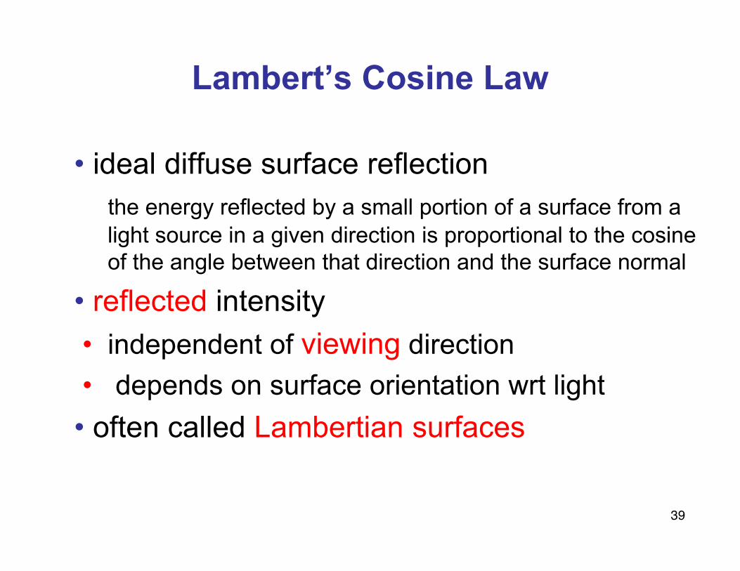
Lambert’s Cosine Law

• ideal diffuse surface reflectionthe energy reflected by a small portion of a surface from alight source in a given direction is proportional to the cosineof the angle between that direction and the surface normal

• reflected intensity

• independent of viewing direction

• depends on surface orientation wrt light

• often called Lambertian surfaces

40

Lambert’s Law

intuitively: cross-sectional area ofthe “beam” intersecting an elementof surface area is smaller for greaterangles with the normal.

41

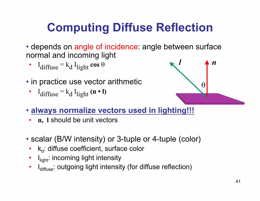
Computing Diffuse Reflection

• depends on angle of incidence: angle between surfacenormal and incoming light• Idiffuse = kd Ilight cos θ

• in practice use vector arithmetic• Idiffuse = kd Ilight (n • l)

• always normalize vectors used in lighting!!!• n, l should be unit vectors

• scalar (B/W intensity) or 3-tuple or 4-tuple (color)• kd: diffuse coefficient, surface color• Ilight: incoming light intensity• Idiffuse: outgoing light intensity (for diffuse reflection)

nl

θ

42

Diffuse Lighting Examples

• Lambertian sphere from several lightingangles:

• need only consider angles from 0° to 90°• why?

• demo: Brown exploratory on reflection• http://www.cs.brown.edu/exploratories/freeSoftware/repository/edu/brown/cs/ex

ploratories/applets/reflection2D/reflection_2d_java_browser.html