Light Water Reactor Sustainability Program Integration of ...

INL/EXT-16-39015

Light Water Reactor Sustainability Program

Integration of Human Reliability Analysis Models into the Simulation-Based

Framework for the Risk-Informed Safety Margin Characterization Toolkit

June 2016

U.S. Department of Energy

Office of Nuclear Energy

DISCLAIMERThis information was prepared as an account of work sponsored by an agency of the U.S. Government. Neither the U.S. Government nor any agency thereof, nor any of their employees, makes any warranty, expressed or implied, or assumes any legal liability or responsibility for the accuracy, completeness, or usefulness, of any information, apparatus, product, or process disclosed, or represents that its use would not infringe privately owned rights. References herein to any specific commercial product, process, or service by trade name, trade mark, manufacturer, or otherwise, does not necessarily constitute or imply its endorsement, recommendation, or favoring by the U.S. Government or any agency thereof. The views and opinions of authors expressed herein do not necessarily state or reflect those of the U.S. Government or any agency thereof.

INL/EXT-16-39015

Integration of Human Reliability Analysis Models into the Simulation-Based Framework for the Risk-

Informed Safety Margin Characterization Toolkit

Ronald Boring1, Diego Mandelli1, Martin Rasmussen2, Sarah Herberger1,Thomas Ulrich1, Katrina Groth3, and Curtis Smith1

1Idaho National Laboratory2NTNU Social Research

3Sandia National Laboratories

June 2016

Idaho National LaboratoryIdaho Falls, Idaho 83415

http://www.inl.gov

Prepared for theU.S. Department of EnergyOffice of Nuclear Energy

Under DOE Idaho Operations OfficeContract DE-AC07-05ID14517

(This page intentionally left blank)

iii

ABSTRACT

This report presents an application of a computation-based human reliability analysis framework called the Human Unimodel for Nuclear Technology to Enhance Reliability (HUNTER), a method developed as part of the Risk Informed Safety Margin Characterization (RISMC) pathway within the U.S. Department of Energy’s Light Water Reactor Sustainability Program that aims to extend the life of the currently operating fleet of U.S. commercial nuclear power plants. HUNTER is a flexible hybrid approach that functions as an framework for dynamic modeling, including a simplified model of human cognition—a virtual operator—that produces relevant outputs such as the human error probability (HEP), time spent on task, or task decisions based on relevant plant evolutions. HUNTER is the human reliability analysis counterpart to the Risk Analysis and Virtual ENvironment (RAVEN) framework used for dynamic probabilistic risk assessment. Although both RAVEN and HUNTER are still under various stages of development, this report presents a successfully integrated and implemented RAVEN-HUNTERinitial demonstration. The demonstration in this report centers on a station blackout scenario, using complexity as the sole virtual operator performance-shaping factor (PSF). The implementation of RAVEN-HUNTER can be readily scaled to other nuclear power plant scenarios of interest and include additional PSFs in the future.

iv


v

ACKNOWLEDGMENTS

We express our sincere thanks for textual reviews and inputs from Gordon Bower, Nancy Lybeck, Kateryna Savchenko, and Jeff Einerson at INL.

vi


vii

CONTENTS

ACKNOWLEDGMENTS .............................................................................................................. v

ACRONYMS............................................................................................................................... xiii

1. INTRODUCTION ................................................................................................................... 11.1 Human Unimodel for Nuclear Technology to Enhance Reliability .................................. 11.2 Outline of Report ............................................................................................................... 2

2. BACKGROUND ON HUMAN RELIABILITY ANALYSIS ............................................... 52.1 Traditional Human Reliability Analysis ............................................................................ 52.2 Computation-Based HRA.................................................................................................. 62.3 The Need for Computation-Based Human Reliability Analysis ....................................... 7

3. RAVEN SIMULATION FRAMEWORK............................................................................. 133.1 Background...................................................................................................................... 133.2 Background on Risk-Informed Safety Margin Characterization..................................... 143.3 RELAP-7 ......................................................................................................................... 153.4 Simulation Controller ...................................................................................................... 16

4. HUMAN RELIABILITY SUBTASK PRIMITIVES............................................................ 194.1 GOMS-HRA.................................................................................................................... 19

4.1.1 Introduction ............................................................................................................... 194.1.2 The GOMS Method................................................................................................... 194.1.3 Adapting KLM .......................................................................................................... 20

4.1.3.1 Defining Operators .............................................................................................. 204.2 Defining GOMS HRA Task Level Primitives................................................................. 224.3 Discussion........................................................................................................................ 24

5. MODELING PERFORMANCE SHAPING FACTORS...................................................... 255.1 Complexity ...................................................................................................................... 255.2 Complexity in Traditional HRA ...................................................................................... 255.3 Advantages of Modeling Complexity in CBHRA........................................................... 255.4 Challenges in Modeling Complexity in CBHRA ............................................................ 265.5 Suggested Solution .......................................................................................................... 27

5.5.1 Autopopulation.......................................................................................................... 275.5.2 Prepopulation ............................................................................................................ 285.5.3 Comparison ............................................................................................................... 29

5.6 General Form of Complexity Modeling .......................................................................... 29

6. QUANTIFYING THE HUMAN ERROR PROBABILITY ................................................. 336.1 Generic Approach to Quantification................................................................................ 336.2 Nominal Human Error Probability .................................................................................. 33

6.2.1 GOMS-HRA Nominal Error ..................................................................................... 336.2.2 SPAR-H Nominal Error ............................................................................................ 34

7. SIMULATION CASE STUDY: STATION BLACKOUT................................................... 397.1 Station Blackout Background .......................................................................................... 397.2 Simplified Plant System .................................................................................................. 39

viii

7.3 Station Blackout Scenario................................................................................................ 417.4 Stochastic Parameters ...................................................................................................... 437.5 RAVEN Implementation ................................................................................................. 43

7.5.1 Component Modeling................................................................................................ 457.5.2 RAVEN Control Logic.............................................................................................. 457.5.3 Transient Example..................................................................................................... 46

7.6 GOMS-HRA Procedure Primitives ................................................................................. 487.6.1.1 Defining Nominal Timing Data and HEPs.......................................................... 50

7.7 Autocalculating the Complexity Performance Shaping Factor ....................................... 537.7.1 SPAR-H Complexity................................................................................................. 537.7.2 Calculating Complexity............................................................................................. 55

7.7.2.1 Linear Form of Complexity................................................................................. 557.7.2.2 Stochastic Form of Complexity........................................................................... 577.7.2.3 Comparing the Linear and Stochastic Models of Complexity ............................ 61

7.8 Quantifying Operator Performance ................................................................................. 637.9 Implementation of HUNTER Modules within RAVEN ................................................. 657.10 Results ........................................................................................................................... 667.11 Analysis of Scenario 1a ................................................................................................. 687.12 Scenario 1b .................................................................................................................... 697.13 Scenario 1c .................................................................................................................... 697.14 Scenario 2a .................................................................................................................... 707.15 Scenario 2b: LOOP/LODG/LOB .................................................................................. 707.16 Scenario 2b (mod) ......................................................................................................... 717.17 Fixed vs. Randomly Generated Timings ....................................................................... 71

8. CONCLUSIONS ................................................................................................................... 748.1 Accomplishments of HUNTER Modeling ...................................................................... 748.2 Limitations of HUNTER Modeling................................................................................. 748.3 Future Research on Quantification .................................................................................. 75

8.3.1 Background ............................................................................................................... 758.3.2 Bayesian Network Basic Concepts ........................................................................... 758.3.3 Dynamic Belief Networks......................................................................................... 778.3.4 Advantages of BNs to Enable CBHRA..................................................................... 788.3.5 BNs for GOMS-HRA Primitives in HUNTER......................................................... 78

8.4 Future Research on Empirical Data Collection ............................................................... 808.4.1 HRA Empirical Databases ........................................................................................ 808.4.2 SACADA .................................................................................................................. 808.4.3 KAERI....................................................................................................................... 808.4.4 HRA Data Studies at Norwegian University of Science and Technology................ 80

8.5 Future Research Demonstrations of HUNTER ............................................................... 81

9. REFERENCES ...................................................................................................................... 82

APPENDIX A: LIST OF HUNTER PUBLICATIONS ............................................................... 89

ix

FIGURES

Figure 1. Framework for computation-based HRA (from Boring et al., 2015).............................. 1 Figure 2. A common quantification approach in traditional or static HRA.................................... 5 Figure 3. The Linear task path of traditional static HRA, modeled through an event tree............. 6 Figure 4. CBHRA allows for multiple outcomes from each task, leading to a large

number of possible ways a scenario can play out. ........................................................... 7 Figure 5. The non-effect of time on the error estimate in static HRA. ......................................... 10 Figure 6. The effect of time on the error estimate in dynamic HRA. ........................................... 11 Figure 7. Hypothetical subtask HEP calculation for a dynamic event progression...................... 12 Figure 8. Scheme of RAVEN statistical framework components. ............................................... 13 Figure 9. Overview of the RISMC modeling approach................................................................ 14 Figure 10. RAVEN simulation controller scheme. ....................................................................... 18 Figure 12. Quantification approach in traditional static HRA...................................................... 28 Figure 14. Overall HEP calculation based on the nominal HEP and PSFs (from Boring,

2009). ............................................................................................................................. 33 Figure 15. Comparison of nominal HEPs for SPAR-H and GOMS-HRA. .................................. 37 Figure 16. Scheme of the TMI PWR benchmark (from Nuclear Energy Agency, 1999). ........... 40 Figure 17. Scheme of the electrical system of the PWR model (from Nuclear Energy

Agency, 1999)................................................................................................................ 41 Figure 18. Sequence of events for the SBO scenario considered. ................................................ 42 Figure 19. Screenshot of the PWR model of RELAP-7 using PEACOCK. ................................. 44 Figure 20. Core zone correspondence (left) and assembly relative power (right)........................ 44 Figure 21. Example of LOOP scenario followed by DGs failure using the RELAP-7 code........ 47

Figure 22. Plot of the pdfs of PG time recovery (tPG_rec) and DG time recovery (tDG_rec)........................................................................................................................ 47

Figure 23. Plot of the pdfs of battery life (tbatt_fail) and battery recovery time (tbatt_rec)...................................................................................................................... 48

Figure 24. Procedure level primitive decomposition into task level primitive example. ............. 49 Figure 25. Distribution of complexity when using equaiton (12) and the variable

distributions from Table 23............................................................................................ 61 Figure 26. Temporal evolution of the complexity multiplier for the linear case. ......................... 62 Figure 27. Temporal evolution of the complexity multiplier for the stochastic case. .................. 63 Figure 26. HUNTER modeling scheme for each procedure......................................................... 65

x

Figure 27. HUNTER modeling scheme for each procedure step. ................................................ 66 Figure 28. Plot of Scenario 1. ....................................................................................................... 67 Figure 29. Plot of Scenario 2. ....................................................................................................... 67 Figure 30. Distribution of the timing to perform PTA procedure (Scenario 1a). ......................... 68 Figure 31. Distribution of the timing to perform SBO procedure (Scenario 1a).......................... 69 Figure 32. Distribution of the timing to perform SBO procedure (Scenario 1b).......................... 69 Figure 33. Distribution of the timing to perform SBO procedure (Scenario 1c). ......................... 70 Figure 34. Distribution of the timing to perform the sequence of PTA and SBO

procedures (Scenario 2a)................................................................................................ 70 Figure 35. Distribution of the timing to perform PTA + SBO procedures (Scenario 2b). ........... 71 Figure 36. Distribution of the timing to perform PTA + SBO procedures (Scenario 2b)

with higher nominal HEP value = 0.01......................................................................... 71 Figure 37. Distribution of the timing to perform PTA + SBO procedures using the linear

complexity model for LOOP+LODG with (left) and without (right) LOB................... 72 Figure 38. A simple BN example using SPAR-H PSFs and other shaping factors. ..................... 76 Figure 39. Verify mini-BN for use within HUNTER (adapted from Zwirglmaier et al., in

press). ............................................................................................................................. 79

xi

TABLES

Table 1. Fitting of distributions to GOMs task level primitive “Ac” using an MLE. .................. 23 Table 2. Results of the fitting of GOMs task level primitives using an MLE, with 5th and

95th percentiles displayed.............................................................................................. 24 Table 3. Spearman rank-order correlations between complexity and other PSFs in SPAR-

H (adapted from Boring, 2010)...................................................................................... 30 Table 4. Dynamic functions that may affect the general calculation of the PSF.......................... 31 Table 5. GOMS-HRA nominal HEP values for the task level primitives. ................................... 35 Table 6. SPAR-H nominal HEP values for the task level primitives. .......................................... 36 Table 7. Power distribution factor for representative channels and average pellet power. .......... 45 Table 8. Pseudo code 1: Battery system control logic .................................................................. 46 Table 9. Pseudo code 2: DG and PG control logic ...................................................................... 46 Table 10. Pseudo code 3: AC power status control logic ............................................................. 46 Table 11. Probability distribution functions for sets of uncertainty parameters........................... 48 Table 12. Procedure level primitive definitions............................................................................ 49 Table 13. Generic procedure level primitive mapping to task level primitives............................ 50 Table 14. Example mapping of procedure step to procedure and task level primitives. .............. 50 Table 15. SBO Step 5 showing mapping of Ensure procedure level primitive. ........................... 51 Table 16. Post trip actions and station blackout procedures mapped to procedure and task

level primitives............................................................................................................... 52 Table 17. Procedure steps and associated task level primitives mapped onto the main

events of the modeled scenario and the estimated timing data. ..................................... 53 Table 18. SPAR-H worksheet excerpt for the Complexity PSF level multipliers........................ 54 Table 19. Fitting of distributions to SPAR-H frequency data from Boring et al. (2006) ............. 54 Table 20. A 20-task breakdown of complexity for a station blackout event. ............................... 55 Table 21. Regression output with complexity as the dependent variable, based on the data

from Table 20................................................................................................................. 57 Table 22. Normalized complexity values for the task level primitives in the modeled

scenario. ......................................................................................................................... 58 Table 23. Distributions associated with the variables for the SBO simulation. ........................... 59 Table 24. One iteration of the SBO procedures and the assigned values ..................................... 59 Table 25. A sample of 9 representative observations of the 5,000 regression coefficients

generated from fitting the simulation data that is similar to Table 24. .......................... 60

xii

Table 26. The parameters of the normal distributions associated with their respective coefficients. .................................................................................................................... 60

Table 27. GOMS-HRA and SPAR-H HEP values for the task level primitives in the modeled scenario. .......................................................................................................... 64

xiii

ACRONYMS

AC Alternating CurrentAIC Akaike Information CriterionBIC Bayesian Information CriterionBN Bayesian NetworkBBN Bayesian Belief NetworkCBDT Cause Based Decision TreeCBHRA Computation-Based Human Reliability AnalysisCPM-GOMS Cognitive, Perceptual, and Motor-GOMSDC Direct CurrentDG Diesel GeneratorDOE Department of EnergyECCS Emergency Core Cooling SystemEOP Emergency Operating ProceduresGLEAN GOMS Language Evaluation and AnalysisGOMS Goals, Operators, Methods, Selection rulesHEART Human Error Assessment and Reduction TechniqueHEP Human Error ProbabilityHERA Human Event Repository and AnalysisHFE Human Failure EventHMI Human-Machine InterfaceHRA Human Reliability AnalysisHUNTER Human Unimodel for Nuclear Technology to Enhance Reliability INL Idaho National LaboratoryKAERI Korea Atomic Energy Research InstituteKLM Keystroke Level ModelLOB Loss of BatteryLODG Loss of Diesel GeneratorLOOP Loss of Offsite PowerLWRS Light Water Reactor SustainabilityMLE Maximization Likelihood EstimateMOOSE Multi-Physics Object-Oriented Simulation EnvironmentMSLB Main Steam Line BreakNGOMS Natural Goals, Operators, Methods, Selection rulesNPP Nuclear Power PlantaNRC Nuclear Regulatory CommissionOECD Office of Economic Cooperation and Developmentpdf Probability Density FunctionPG Power GridPLP Procedure Level PrimitivePRA Probabilistic Risk AssessmentPSF Performance Shaping FactorPTA Post Trip ActionPWR Pressurized Water ReactorRAVEN Risk Analysis and Virtual ENvironment

xiv

RISMC Risk Informed Safety Margin CharacterizationRO Reactor OperatorROM Reduced Order ModelSACADA Scenario Authoring, Characterization, and Debriefing, ApplicationSBO Station BlackoutSHERPA Systematic Human Error Reduction and Prediction ApproachSME Subject Matter ExpertSPAR-H Standardized Plant Analysis Risk-Human Reliability AnalysisTHERP Technique for Human Error Rate PredictionTMI Three Mile IslandTLP Task Level PrimitiveU.S. United States

1

1. INTRODUCTION

1.1 Human Unimodel for Nuclear Technology to Enhance Reliability

This report presents an application of a computation-based human reliability analysis (CBHRA) framework called the Human Unimodel for Nuclear Technology to Enhance Reliability (HUNTER; see Boring et al., 2015). A unimodel—the U in HUNTER—is a simplified cognitive model. Thus, HUNTER represents a simplified cognitive model or a collection of simplified cognitive models to support dynamic risk analysis. HUNTER is a hybrid approach built on past work from cognitive psychology, human performance modeling, and human reliability analysis (HRA). Using these research fields as background, HUNTER functions as a simplified model of human cognition—a virtual operator—that, when combined with a computation engine such as a thermo-hydraulics based nuclear power plant simulation model, can produce outputs such as the human error probability (HEP), time spent on task, or task decisions based on relevant plant evolutions.

HUNTER is flexible in terms of which inputs and cognitive evaluations are used and which outputs it produces. HUNTER has been developed not as a standalone HRA method but rather as a framework that ties together different HRA methods to model dynamic risk of human activities and serve as an interface between HRA and other aspects of the dynamic modeling, such as thermo-hydraulic code, as part of an overall probabilistic risk assessment (PRA). HUNTER is the HRA counterpart to the Risk Analysis and Virtual ENvironment (RAVEN; see Chapter 3)framework in PRA, as depicted in Figure 1. Although both RAVEN and HUNTER are still under various stages of development, this report represents a successfully integrated and implemented RAVEN-HUNTER demonstration. The demonstration in this report centers on a station blackout scenario, but the implementation of RAVEN-HUNTER is scalable to other nuclear power plant scenarios of interest in the future.

Figure 1. Framework for computation-based HRA (from Boring et al., 2015).

CognitiveModels

DataSources

Plant

• Model

2

HUNTER was created with the goal of including HRA in areas where it has not been represented so far and to reduce uncertainty by accounting for human performance more accurately than current HRA approaches. While we have adopted particular methods to build an initial model, the HUNTER framework is intrinsically flexible to new modules that achieve particular modeling goals. Fodor, speaking to the enterprise of cognitive science, suggested that the brain was comprised of many separate functions based in neuroanatomical structures of the brain (1983). He famously termed this clustering of mental systems the modularity of mind, which we here extend to the modularity of models of mind. Computation-based HRA in HUNTER does not consist of a single HRA model or method; rather, it can encompass a number of different HRA approaches that account for different aspects of human performance. A goal of HUNTER is, in fact, to “dynamicize” legacy HRA approaches wherever feasible.

In the present report, the HUNTER implementation has the following goals:

Integration through RAVEN with a high fidelity thermo-hydraulic code capable of modeling nuclear power plant behaviors and transientsConsideration of risk through integration with PRA modelingIncorporation of a solid psychological basis for operator performanceDemonstration of a functional dynamic model of a plant upset condition and appropriate operator response.

This report outlines the effort to develop the HUNTER framework and presents the case study of a station blackout (SBO) scenario to demonstrate the various modules implemented under the initial HUNTER research umbrella.

The HUNTER project is part of the Risk Informed Safety Margin Characterization (RISMC) research pathway within the U.S. Department of Energy’s Light Water Reactor Sustainability (LWRS) program that aims to extend the life of the currently operating fleet of U.S. commercial nuclear power plants. HUNTER has the potential to model risk more accurately across a greater range of scenarios than has been possible with conventional HRA approaches. Additionally, HUNTER provides a crucial connection between RAVEN and human performance, which extends the utility of that modeling code. As such, HUNTER ultimately aims to ensure the continued safety and reliability of currently operating nuclear power plants.

1.2 Outline of Report

This report steps through multiple modules in support of defining and demonstrating the HUNTER framework. The chapters correspond to different modeling modules and are as follows:

Chapter 2 provides background on HRA and, specifically, the necessary transition from traditional, static HRA methods to dynamic or computation-based methodsChapter 3 provides background on RAVEN, which is used as the control logic driver for the thermo-hydraulic code (RELAP-7) used in the nuclear power plant simulations for the demonstration in this report

3

Chapter 4 presents the GOMS-HRA (Goals, Operators, Methods, and Selection rules –Human Reliability Analysis; Boring & Rasmussen, 2016) method used to decompose the station blackout scenario used in the demonstration into standardized task units suitable for task timing and error rate predictionChapter 5 presents a dynamic model for complexity, which serves as a performance shaping factor (PSF) used in quantification of the HEPChapter 6 presents a general approach for dynamic HEP calculationChapter 7 presents the SBO case study, implementation details, and resultsChapter 8 summarizes lessons learned on HUNTER and outlines future research directions.

4


5

2. BACKGROUND ON HUMAN RELIABILITY ANALYSIS

2.1 Traditional Human Reliability Analysis

In HRA, human action or several human actions in a task or scenario are analyzed in terms of the likelihood that an operator or a crew will be successful (often in preventing a potential accident scenario from leading to core damage in a nuclear power plant or another form of major accident). There are dozens of different HRA methods (see Boring, 2012; Spurgin, 2010;Rasmussen, in press), leading to many variations in how HRAs are conducted, but in general the HRA process consists of:

Identifying possible human errors and contributors,Modeling human error, and Quantifying HEPs (Swain, 1990).

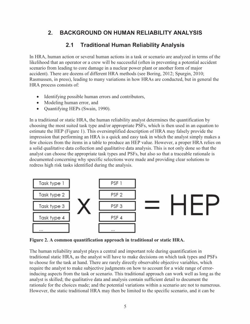
In a traditional or static HRA, the human reliability analyst determines the quantification by choosing the most suited task type and/or appropriate PSFs, which is then used in an equation to estimate the HEP (Figure 1). This oversimplified description of HRA may falsely provide the impression that performing an HRA is a quick and easy task in which the analyst simply makes a few choices from the items in a table to produce an HEP value. However, a proper HRA relies on a solid qualitative data collection and qualitative data analysis. This is not only done so that the analyst can choose the appropriate task types and PSFs, but also so that a traceable rationale is documented concerning why specific selections were made and providing clear solutions to redress high risk tasks identified during the analysis.

Figure 2. A common quantification approach in traditional or static HRA.

The human reliability analyst plays a central and important role during quantification in traditional static HRA, as the analyst will have to make decisions on which task types and PSFs to choose for the task at hand. There are rarely directly observable objective variables, which require the analyst to make subjective judgments on how to account for a wide range of error-inducing aspects from the task or scenario. This traditional approach can work well as long as the analyst is skilled; the qualitative data and analysis contain sufficient detail to document the rationale for the choices made; and the potential variations within a scenario are not to numerous.However, the static traditional HRA may then be limited to the specific scenario, and it can be

Task type 1

Task type 2

Task type 3

Task type 4x

PSF 1

PSF 2

PSF 3

PSF 4HEP

6

difficult to generalize the results to other scenarios. In fact, scenario reusability in HRA remains a highly coveted but still elusive goal.

In traditional static HRA, a scenario is established either at the beginning of the analysis, or one is already predetermined through a larger risk analysis process such as a PRA. A variety of methods—such as task analysis, error trees, event trees, and timeline analyses—are then used to determine the necessary and relevant human error information contained in the scenario and accompanying human actions. The modeling is generally based on a linear path of actions the operator must perform to avoid a major accident (e.g., core damage in the nuclear process control domain; Figure 2). Failures to complete these tasks are commonly referred to as errors of omission. Wrong actions—errors of commission—are often not explicitly included in traditional static HRA.

Figure 3. The Linear task path of traditional static HRA, modeled through an event tree.

2.2 Computation-Based HRA

The approach of CBHRA relies on the creation of a virtual operator that is interfaced with a realistic plant model that can accurately simulate plant thermo-hydraulic physics behavior (Boring et al. 2015). Ultimately, the virtual reactor operator should consist of comprehensive cognitive models comprised of artificial intelligence, though at this time a much more simplified operator model is used to simulate performance of a typical operator. CBHRA is a merger between an area where HRA has previously been represented—probabilistic risk models—and an area where it has not—realistically simulated plant models through mechanistic thermal-hydraulic multi-physics codes. Through this approach, it is possible to evaluate a much broader spectrum of scenarios, both those based on previous experience and those that are unexampled, i.e., that have not been assessed with static HRA.

This is a promising path to advance the methodology of HRA, but there are numerous challenges that must be overcome before a fully functioning plant simulation including a virtual operator model becomes realized. In CBHRA, a scenario can be rapidly simulated thousands of times (see Figure 4), which renders individual subjective evaluations by a human reliability analyst during each simulation run impractical. Unfortunately, most of the PSFs in current HRA methods are operationalized and described in a way that suits subjective evaluations from the analyst, which

Task 1

Success

=> Task 2 =>- Task 3

SucLess

hjilure

ailure

Fuilue

Success

FailureFailure

Failure

7

presents challenges to translate the static optimized methods to a coding scheme that canautomatically and dynamically set the PSF at the correct level during simulation runs.Despite these challenges, CBHRA is worthy to pursue because it will be able to include significantly more paths than the limited paths seen in traditional static HRA. CBHRA may alsoinclude emergent changes throughout the scenario, ultimately providing a better quantification of the risk than using pre-scripted risk trees.

Figure 4. CBHRA allows for multiple outcomes from each task, leading to a large number of possible ways a scenario can play out.

2.3 The Need for Computation-Based Human Reliability Analysis

PRA models plant safety through quantitative risk measures. Typically measured as conditional core damage frequency or probability, the output of the PRA accounts for the likelihood of damage to the plant fuel, containment, or surrounding environment in the event of failures to specific hardware systems. Many hardware systems are operated by humans; as such, human actions or inactions are integral to the overall analysis of risk.

Mosleh (2014) and Coyne and Siu (2013) have emphasized the importance of computational approaches to PRA. These approaches, which use dynamic simulations of events at plants, potentially provide greater accuracy in overall risk modeling. Here we explore the human side ofdynamic PRA. The key elements of dynamic or computation-based HRA are:

Success

Failure

8

Use of computational techniques, namely simulation and modeling, to integrate virtual operator models with virtual plant modelsDynamic modeling of human cognition and actionsIncorporation of these respective elements into a PRA framework.

The goal of the present research is to achieve a high fidelity causal representation of the role of the human operator at the plant. By better accounting for human actions, the uncertainty surrounding PRA can be reduced. Additionally, by modeling human actions dynamically, it is possible to model types of activities and events in which the human role is currently not clearly understood or predicted, e.g., unexampled events such as severe accidents. The ability to simulate the role of the human operator complements and, indeed, greatly enhances other PRA modeling efforts.

A significant influence on plant behavior and performance comes from the human operators who use that plant. The computational engine of the virtual plant model therefore needs to interface with a virtual operator that models operator performance at the plant. In current nuclear power plants (NPPs), most plant actions are manually controlled from the control room by reactor operators (ROs) or locally at the physical plant systems by field operators. Consequently, in order to have a non-idealized model of plant performance, it is necessary to account for those human actions that ultimately control the plant. A high fidelity representation of an NPP absolutely requires an accurate model of its human operators in order to faithfully represent real-world operation.

While it is tempting simply to script human actions at the NPP according to operating procedures, there remains considerable variability in operator performance despite the most formalized and invariant procedures to guide activities (Forester et al., 2014). Human decision making and behavior are influenced by a myriad of factors at and beyond the plant. Internal to the plant, the operators may be working to prioritize responses to concurrent demands, to maximize safety, and/or to minimize operational disruptions. While it is a safe assumption that the operators will act first to maintain safety and then electricity generation, the way he or she accomplishes those goals may not always flow strictly from procedural guidance. Operator expertise and experience may govern actions beyond rote recitation of procedures. As a result, human operators may not always make decisions and perform actions in a seemingly rational manner. Modeling human performance without considering the influences on the operators will only result in uncertain outcomes.

Conventional, static HRA supports PRA by considering the human contribution to overall system risk. HRA may be successfully integrated into PRA in a well-established process (Bell & Swain, 1983; EPRI, 1992; IEEE, 1997). The key to this integration is the human failure event (HFE), which represents a clustering of human activities related to the operation of a particular system or component. The HFE can be quantified using any of a number of HRA methods (for recent surveys, see Bell & Holroyd, 2009; Chandler et al., 2006; and Forester et al., 2006). The HFE is integrated into the event trees used in the PRA. Often the clustering of activities under the HFE is done using fault tree logic. In practice, the HFE is defined as the entirety of human actions related to the human interaction with a particular system. In other words, the HFE is

9

defined top-down, from the PRA level of interest, to encompass all human actions that can contribute to the fault of a component or system modeled in the PRA.

Static HRA mimics the predominance of static PRA. The key point in static HRA and PRA is that events are analyzed for an assumed, e.g., typical, window of time. The HFE for static HRA does not change as a function of time or the event progression; the event sequences are fixed in the HRA, and the analysis represents a snapshot of time. Either the analysis represents a very generic context in which the event would occur, or the analysis is agnostic to time, meaning that time evolution is simply not factored into the calculation of the HEP. Other PSFs apart from time drive the quantification of the HEP.

As Boring, Joe, and Mandelli (2015) point out, widely used HRA methods, such as the Standardized Plant Analysis Risk-Human Reliability Analysis (SPAR-H) method (Gertman et al., 2005), are static. They do not provide a dynamic account of human actions or how the PSFs can dynamically modify the HEP over time. Building on the three basic elements of HRA outlined in Section 2.1, SPAR-H and similar methods generally entail three steps:

Identification of human failure events (often through task analysis),Assessment of context (e.g., via assigning states to PSFs and other contextual factors), andComputation of an HEP (generally via an equation defining how the state of the contextual variables, e.g. PSFs, changes a nominal HEP for the task and/or HFE).

A human reliability analyst using SPAR-H would first screen for HFEs involving risk significant human errors and successful human actions. The analyst would then use SPAR-H to model and quantify the operator diagnoses (e.g., cognitive activities) and operator actions (e.g., behaviors) associated with the identified HFEs, starting with nominal HEPs, and then multiplying the nominal HEPs by any or all of the eight PSF modifiers provided in the method.

SPAR-H calculates an HEP based on a static rating of PSFs. In essence:

HEPHFE = f(HEPnominal | PSFs) (1)

where:

HEPHFE is the human error probability for the human failure event,HEPnominal is the nominal or default HEP provided in the method, andPSFs is the set of performance shaping factors that is considered in the method.

Of course, different HRA methods have vastly different approaches to estimating HEPs, and not all methods will formally enlist nominal HEPs or PSFs. Conceptually, however, the point remains that the HEP is a function of a particular probabilistic approach given some context that affects operator performance. Given this simplified approach, once the HEP is calculated as a function of how PSFs modify the nominal HEP, it remains unchanged over the (time) duration of the HFE (see Figure 5).

10

Figure 5. The non-effect of time on the error estimate in static HRA.

It should be noted that SPAR-H does, indeed, model time as a PSF. Specifically, SPAR-Hanalyzes the impact of available time to complete the task on the HEP. A shorter window of time degrades the operators’ performance or at least their ability to complete the task successfully. The modeling of time as a PSF is, however, not the same as dynamic HRA. Time, as modeled in SPAR-H and other HRA methods, is dynamically invariant for the HFE. For the specific HFE being analyzed, the analyst will not typically look at a range of time windows or how that time window changes throughout alternate event evolutions. Time, in static HRA, is simply a snapshot of an available resource the operator needs, which is firmly fixed in a predefined HFE in the PRA.

The preceding discussion has centered on HFE modeling and HEP quantification for conventional HRA, which are static in nature. Once the overall system is modeled, including HFEs, the HFEs do not change as a result of the event progression. Dynamic HRA does not rely on a fixed set of event and fault trees to model event outcome. Rather, it builds the event progression dynamically, as a result of ongoing actions (Acosta & Siu, 1993). The dynamic approach in PRA has proved especially useful for modeling beyond design basis accidents, where not all failure combinations (and, importantly, not all recovery opportunities) can be anticipated or have been included in the static model. Additionally, the failure of multiple components or unusual sequences of faults, even within design basis, may challenge the fidelity of the static PRA model. While such events are rare, dynamic modeling affords the opportunity to anticipate such permutations and address them in a risk-informed manner should they occur.

Boring (2007), among others, explains the conceptual shift from static HRA to dynamic HRA. Key aspects of this shift are the transition from predictions based on fixed models of accident sequences into predictions based on direct simulation of an accident sequence, with explicit

0.01

0.008 -

Lif 0.006 -0_u..1x 0.004 -

0.002 -

o1 5 9 13 17 21 25 29

Time

11

consideration of timing of key events. For HRA to fit into this dynamic framework, the models must follow a parallel path, shifting away from estimating the probability of a static event, and into simulating the multitude of possible human actions relevant to an event.

Traditional static HRA attempts to directly estimate or assign probabilities to defined HFEs. Example HFEs are “failure to initiate feed and bleed” and “failure to align electrical bus to alternative feed.” In this new dynamic HRA framework, the focus shifts to simulating the human performance within a dynamic PRA framework and using the results of those simulations to assign the HEP. Dynamic HRA yields HFEs such as “failure to initiate feed and bleed over time.”

In essence, the HEP that is quantified varies over time as PSFs change in their influence:

HEPdynamic = f(HEPnominal | PSF(t)) (2)

where t is time. The PSFs change their influence on the HEP over time, because the PSFs change states as the context of the event unfolds.

This dynamic formulation of the HEP in Equation 2 is similar to the static formulation in Equation 1 in that the HEP is quantified as a function of the nominal HEP as adjusted by PSFs. The key difference is that both the state of the PSFs and the influence of the PSFs can change over time. The final effect is that the HEP varies over time (see Figure 6).

Figure 6. The effect of time on the error estimate in dynamic HRA.

As depicted in Figure 7, dynamic HRA must account for subtasks. Figure 7 may represent a single HFE, which is comprised of several time segments and several subtasks. The current-

0.01 •

0.008

%0.006-0

o_w 0.004

0.002

1 5 9 13 17 21 25 29

Time

12

moment quantification varies not only as a function of time but also as a function of the subtasks carried out by the operators. Additionally, as discussed in Boring (2015), there is a dynamic dependence caused by the lingering effects of PSFs across subtasks. Each subtask is not a fresh slate in terms of influences on performance. PSFs like stress do not subside instantly simply because the source or cause of that stress has disappeared. Rather, PSFs have a momentum that must be factored into the evolution of the event. The subtasks may represent decision or critical performance points where the outcome can change as a result of PSFs. It is therefore not feasible to model at the HFE level, where important influences on the event outcome may be overlooked. Instead, dynamic HRA requires subtask granularity.

Figure 7. Hypothetical subtask HEP calculation for a dynamic event progression.

As discussed in Boring (2015), most HRA methods do not provide clear guidance on defining HFEs or for decomposing these events into meaningful subtasks. This serves as a significant disconnect between the task analysis approaches common to human factors and the HFEs used by HRA, and it can be especially difficult when a task analysis is available to use it to build an HFE. It is generally adequate for static HRA to be at the HFE level. The HFE is defined by the PRA in a top-down manner reflecting the failure of a system with a possible human contribution. The output of the HFE is the HEP, which serves as the input in the overall PRA model. It is, however, inadequate for dynamic HRA to be modeled only at the HFE level. It must account for the nuances of operator actions that can change across subtasks or steps in a procedure. For this reason, it is necessary to define an approach that adequately accounts for subtask modeling in order to allow dynamic operator modeling.

Tasks

C D0.1

0.095

0.09

0.085

0.08

0.075

0.07 •

0.065

0.06

0.055

0.05

0.045

0.04

0.035

0.03

0.025

0.02

0.015

0.01

0.005

0 11 2 4 5 6 7 8 9

Tirne (rin)

10

13

3. RAVEN SIMULATION FRAMEWORK

3.1 Background

RAVEN (Risk Analysis and Virtual ENviroment; Rabiti et al., 2013; Mandelli et al., 2013) is a software framework that acts as the control logic driver for the thermal-hydraulic code RELAP-7, a newly developed software at Idaho National Laboratory (INL). RAVEN is also a multi-purpose PRA code that allows for probabilistic analysis of complex systems. It is designed to derive and actuate the control logic required to simulate both plant control system and operator actions (e.g., guided procedures) and to perform both Monte-Carlo sampling (Rabiti, Mandelli, Alfonsi, Cogliati, & Kinoshita, 2013) of random distributed events and dynamic branching-typeanalyses (Alfonsi et al., 2014).

The RAVEN statistical framework is a recent add-on to the overall RAVEN package that allows the user to perform generic statistical analysis. By statistical analysis we include:

Sampling of codes, either stochastic (e.g., Monte-Carlo (Marseguerra, Zio, Devooght, & Labeau, 1998) and Latin Hypercube Sampling (Helton & Davis, 2003) or deterministic (e.g., grid and Dynamic Event Tree; Amendola & Reina, 1984)Generation of Reduced Order Models (Abdel-Khalik, Bang, Kennedy, & Hite, 2012),also known as Surrogate modelsPost-processing of the sampled data and generation of statistical parameters (e.g., mean, variance, covariance matrix).

Figure 8. Scheme of RAVEN statistical framework components.

Figure 8 shows a general overview of the elements that comprise the RAVEN statistical framework:

L Code

Run 1

L L

Code

Interfaces

External ROM

\l/

CPU

Node 1

Code CPU

Run 2 \ -In Node

Code

Run N

I CPUNode N

RAV E N

Samplers

Post-Processing

and

Data Mining

module

Database manager

HDF5 Hierarchical Storing Structure

DET

Database

Interface

Output PRA

Database Database

LProbability

Engine

14

Model: it represents the pipeline between input and output space. It comprises both codes (e.g., RELAP-7) and also Reduced Order Models Sampler: it is the driver for any specific sampling strategy (e.g., Monte-Carlo, LHS, DET)Database: the data storing entityPost-processing module: the module that performs statistical analyses and visualizesresults.

3.2 Background on Risk-Informed Safety Margin Characterization

The RISMC approach employs both deterministic and stochastic methods in a single analysis framework (see Figure 9). In the deterministic method set we include:

Modeling of the thermo-hydraulic behavior of the plant (Mandelli, et al., 2015)Modeling of external events such as flooding (Prescott, Smith, & Sampath, 2015)Modeling of the operator responses to the accident scenario (Boring et al., 2014; Boring et al., 2015).

Figure 9. Overview of the RISMC modeling approach.

Note that deterministic modeling of the plant or external events can be performed by employing specific simulator codes but also surrogate models, known as reduced order models (ROM). ROMs would be employed in order to decrease the high computational costs of employed codes.In addition, multi-fidelity codes can be employed to model the same system; the idea is to switch from low-fidelity to high-fidelity code when higher accuracy is needed (e.g., use low-fidelity codes for steady-state conditions and high-fidelity code for transient conditions).

Deterministic modeling

Plant modeling

External event modeling

4.

Stochastic modeling

Identify uncertain parametersand associate a pdf

-VStochastic a ysisa n ie)

Sample the pdfs

Run N times systemsimulation code(s)

Evaluate desired FOMs

Data post-processing

15

On the other hand, in the stochastic modeling we include all stochastic parameters that are of interest in the PRA such as:

Uncertain parametersStochastic failure of system/components.

As mentioned earlier, the RISMC approach heavily relies on multi-physics system simulator codes (e.g., RELAP-7; Anders et al., 2012) coupled with stochastic analysis tools (e.g., RAVEN; Rabiti et al., 2013). From a mathematical point of view, a single simulator run can be represented as a single trajectory in the phase space. The evolution of such a trajectory in the phase space can be described as follows:

( )= ( , , )

(3)

where:

= ( ) represents the temporal evolution of a simulated accident scenario, i.e., ( )represents a single simulation run

is the actual simulator code that describes how evolves in time= ( ) represents the status of components and systems of the simulator (e.g., status of

emergency core cooling system, AC system).

For the scope of this report, it is worth noting that the variable ( ) contains also information about interactions between human models and the considered system. These interactions can be both deterministic (e.g., activation/deactivation of components/systems as requested by the set of procedures) and stochastic (i.e., failure of omission and commission).

By using the RISMC approach, the PRA is performed by (Mandelli, Smith, Alfonsi, & Rabiti, 2014):

1. Associating a probabilistic distribution function (pdf) to the set of parameters (e.g., timing of events)

2. Performing stochastic sampling of the pdfs defined in Step 13. Performing a simulation run given sampled in Step 2, i.e., solve Eq. (3).4. Repeating Steps 2 and 3 M times and evaluating user defined stochastic parameters such

as core damage (CD) probability ( ).

3.3 RELAP-7

The RELAP-7 code (Anders et al., 2012) is the new nuclear reactor system safety analysis codebeing developed at INL. RELAP-7 is designed to be the main reactor system simulation toolkit for the RISMC Pathway of the LWRS Program (Anders et al., 2012). RELAP-7 code development is taking advantage of the progress made in the past several decades to achieve

16

simultaneous advancement of physical models, numerical methods, and software design. RELAP-7 uses INL’s MOOSE (Multi-Physics Object-Oriented Simulation Environment) framework (Prescott, Smith, & Sampath, 2015) for solving computational engineering problems in a well-planned, managed, and coordinated way. This allows RELAP-7 development to focus strictly on system analysis-type physical modeling and gives priority to retention and extension of RELAP5’s multidimensional system capabilities.

A real reactor system is very complex and may contain thousands of different physical components. Therefore, it is impractical to preserve real geometry for the whole system. Instead, simplified thermo-hydraulic models are used to represent (via “nodalization”) the major physical components and describe major physical processes (such as fluid flow and heat transfer). There are three main types of components developed in RELAP-7:

1. one-dimensional (1-D) components,2. zero-dimensional (0-D) components for setting a boundary, and3. 0-D components for connecting 1-D components.

3.4 Simulation Controller

One of the features of RELAP-7 is the capability to control the simulation’s temporal evolution at each time step where, by “control,” we mean a continuous in time interaction between the thermal-hydraulic temporal evolution and the control logic of the plant system. This control action is performed by using two sets of variables (Rabiti et al., 2013):

Monitored variables: the set of observable parameters that are calculated at each calculation step by RELAP-7 (e.g., average clad temperature)Controlled parameters: the set of controllable parameters that can be changed/updated at the beginning of each calculation step (e.g., status of a valve – open or closed –, or pipe friction coefficient).

Starting from Eq. (3), it is possible to split the vector in two parts:

= (4)

The decomposition is carried in such a way that represents the set of unknowns solved by RELAP-7, while represents the set of variables directly controlled and solved by the control logic system (including HUNTER).

Following this new notation, we can say that, for example:

Pressure and temperature in each point of the solution mesh belong to Manual activation of a pump belongs to Activation of high pressure injection system due to trigger in the control logic (low water level in the core) belongs to

17

The governing equation (3) can now be rewritten as follows:

= ( , , )

= ( , , )

(5)

The idea is to use:

(. ) as the calculation performed by RELAP-7(. ) as the calculation performed by the RELAP-7 control logic system (including

HUNTER).

The coupling between (. ) and (. ) exists since they both depend on and . From a HUNTER point of view, can be:

Computations of PSFs as function of the operator working conditions, set of information that is available through the nuclear plant instrumentation, and the human machine interfaceOperators cognitive model solver, the set of Emergency Operating Procedures (EOPs), and in general any set of operator actions (both deterministic and stochastic).

The manipulation of these two data sets of variables is performed by two components of the RAVEN simulation controller (see Figure 10):

RAVEN control logic: is the actual system control logic of the simulation where, based on the status of the system (i.e., monitored variables), it updates the status/value of the controlled parametersRAVEN/RELAP-7 interface: is in charge of updating and retrieving RELAP-7/MOOSE component variables according to the control logic

A third set of variables, i.e., auxiliary variables, allows the user to define simulation specific variables that may be needed to control the simulation. From a mathematical point of view, auxiliary variables are the ones that guarantee the system to be Markovian (Schmidt, 1985), i.e., the system status at time t = t + t can be numerically solved given only the system status at time t = t.

The set of auxiliary variables also includes those that monitor the status of specific control logic set of components (e.g., diesel generators or AC buses) and simplify the construction of the overall control logic scheme of RAVEN.

18

Figure 10. RAVEN simulation controller scheme.

MOOSE

RELAP-7Given the parameter values, the plant status is computed

Plant Status Controlled Parameters

RAVEN / RELAP-7 Interface• Plant status is monitored by a subset of variables

• Controlled parameters are returned to the plant simulation

r

Monitored Controlled

Variables Parameters

RAVEN Control Logic

Based on the status of the system (monitored variables), the control logic

computes the new values of the controlled parameters

19

4. HUMAN RELIABILITY SUBTASK PRIMITIVES

4.1 GOMS-HRA

4.1.1 Introduction

One of the challenges in dynamic HRA is the fact that most HRA methods quantify at the overall task (i.e., HFE) level while subtask quantification will often be required for the dynamic HRA to best follow the scenario as it develops. In an attempt to overcome this challenge, we developed anew HRA approach through categorizing subtasks and linking them to HEPs (Boring & Rasmussen, 2016). This chapter introduces this approach. Although we present a new HRA approach, it bridges several existing concepts from other HRA methods. The purpose of developing this new approach was to allow us to anchor our analyses on subtasks as required by CBHRA, because existing HRA methods did not—in the authors’ views—adequately address subtask analysis.

4.1.2 The GOMS Method

The Goals, Operators, Methods, and Selection rules (GOMS) method was first developed by Card, Moran, and Newell (1983). Goals represent the high level tasks the human seeks to complete, Operators are the available actions the human can take, Methods are the steps or subgoals the human takes toward completing Goals, and Selection rules are the decisions the humans make. GOMS has been used extensively in human factors as a way to model proceduralized activities. It shares underpinnings with task analysis in that it breaks human actions into a series of subtasks. By cataloging particular types of actions, it is possible to predict human actions or task durations. GOMS has also been used in the human factors community to model user interactions with human-computer interfaces. The predictive abilities of GOMS provide an alternative to user studies, but GOMS has been criticized for being time consuming and labor intensive to model (Rogers, Sharp, and Preece, 2002). With the advent of discount usability methods centered on streamlined and cost-efficient data collection for user studies (Nielsen, 1989), the popularity of GOMS modeling as an alternative to such studies has declined.

The simplest rendition of GOMS, the Keystroke-Level Model (KLM; Card, Moran, and Newell, 1980) provides timing data for each type of task, thus making it possible when mapping human actions to predict how long certain activities will take. This approach proved instructive for repetitive tasks like call center operations, where each scripted action could be translated into its overall duration. Thus, it was possible to determine processes or even software use sequences that were inefficient. KLM became a tool for human factors, allowing researchers to optimize human-computer interfaces. Such optimizations became the poster child of human factors, because it was easy to map the repetitive tasks to cost and thereby achieve cost savings with more efficient processes and interfaces. Usability engineering still lives under the shadow of the easy cost savings realized through KLM, and it can be difficult to cost-justify other human factors methods in comparison.

KLM focuses entirely on the operators in GOMS and presents the following list of Operators and corresponding duration times:

20

Keystroke of Button Press (K): t = [0.08s, 1.20s], suggesting a time (t) range from 0.8 to 1.2 seconds (s), depending on the proficiency of the computer userPointing to a Target on a Display with a Mouse (P): t = 1.10sHoming of the Hands (H): t = 0.40sDrawing Line Segments or Precision Work on the Computer Screen (D): t = 0.9n +0.16le, considering the number of line (n) segments and the length (l) of the line in centimetersMentally Preparing for Executing Actions (M): t = 1.35sResponse by the System (R): t = tR, which is the response time (tR) in seconds

KLM builds on task analysis by classifying each human task according to the above Operators. The total duration for the task is the sum of the durations for all subtasks denoted by Operators.Additional and considerably more complex models of GOMS have been developed (see Kieras, 2004, for a review). For example, Cognitive, Perceptual, and Motor (CPM)-GOMS provides a basic model of human cognition to predict task times (Gray, John, and Atwood, 1993), and Natural GOMS Language (NGOMSL) and, more recently, GOMSL, provide a software language for simulating user actions (Kieras, 2006).

Most notable for the purposes of this paper is the GOMS extension called GOMS Language Evaluation and Analysis (GLEAN; Kieras, 2006). GLEAN, specifically GLEAN4, builds on the EPIC human performance modeling architecture, allowing the system to predict upcoming human actions. The Selection Rules in GLEAN, coupled with the underlying EPIC architecture, allow it to mimic decision making. GLEAN has been used to model errors as defined by deviations from procedural scripts (Wood, 2000). GLEAN is also capable of modeling recovery actions, which are simply defined as new Goals to resume the proper course of action. Curiously, GLEAN has not been used to predict HEPs. That GLEAN can predict humanlike decisions and deviations does not expressly allow it to predict the frequency with which such errors occur. This limitation is common for human performance modeling approaches and represents a significant hindrance to their adoption in dynamic HRA (Boring, Joe, and Mandelli, 2015).

In the remainder of this chapter, we review the possibility of using GOMS as an approach to support dynamic HRA. Specifically, with the focus in GOMS on subtasks and proceduralized activities, could GOMS be a feasible method to model basic human actions in nuclear power applications dynamically? Further, could the GOMS Operators provide a foundation for auto-quantification in dynamic HRA?

4.1.3 Adapting KLM

4.1.3.1 Defining Operators

Because KLM is the simplest implementation of GOMS, we will limit our current exploration to it. KLM is optimized to human-computer interactions, and the limited Operators reflect this application. Because the initial domain for GOMS-HRA will be HRA for U.S. NPPs, KLM already finds itself technologically outpacing control room operations. U.S. nuclear power plants

21

are largely legacy analog or mechanical instrumentation and control systems, with minimal visible digital technology. As such, most of the Operators in KLM need to be adapted to different modes of interaction reflecting earlier technologies. This adaptation should not be self-limiting in the sense that it precludes digital interfaces, which are a nascent technology in control rooms.

A review of existing HRA methods for task primitives to use as supplemental Operators in KLM was conducted. As noted already, most HRA is performed at the HFE or task level, and the methods’ units of analysis are also at the task level. For example, the generic task types found in Human Error Assessment and Reduction Technique (HEART; Williams, 1992) do not decompose to the subtask level suitable for dynamic HRA. Decision tree approaches like Cause Based Decision Tree (CBDT; Parry et al., 1992) or performance shaping factor approaches like SPAR-H (Gertman et al., 2005) do not provide ready task primitives that would align to Operators. Finally, while the Technique for Human Error Rate Prediction (THERP; Swain and Guttman, 1983) method provides subtasks in the form of lookup tables, they are not organized in a fashion that presents a ready Operator model of actions.

To find suitable Operators, error taxonomies were investigated next. The Systematic Human Error Reduction and Prediction Approach (SHERPA; Stanton et al., 2013) is often used in conjunction with hierarchical task analysis to cluster subtasks into meaningful tasks suitable for defining HFEs (Boring, 2015). Error taxonomies, however, identify where the task can fail but not what constitutes the successful task. For example, in the SHERPA taxonomy, there are three types of Retrieval Errors related to failures to obtain necessary information:

R1—Information not obtainedR2—Wrong information obtainedR3—Information retrieval incomplete.

The SHERPA taxonomy does not provide the corresponding correct action for information retrieval, which would be more appropriate as Operators in the KLM adaptation. Nonetheless, the SHERPA taxonomy, by grouping types of errors by human activity, actually provides a template for Operators. Below are the high-level groupings of errors in SHERPA:

Action Errors—Performing the required action incorrectly or failing to perform the actionChecking Errors—Looking for required informationRetrieval Errors—Obtaining required information such as from control room indicatorsInformation Communication Errors—Communicating incorrectly or misunderstanding communicationsSelection Errors—Selecting the wrong value or failing to select a valueDecision Errors—Making wrong decision or failing to make decision.

Note that Selection Errors should not be confused with the Selection rules in GOMS, which are more closely linked to Decision Errors. Note that the final error type—Decision Errors—does not appear in the original SHERPA taxonomy and was added in Boring (2015) in order better to account for cognitive errors. Separate taxonomies of cognitive errors such as found in Whaley et al. (2016) point to the importance of addressing cognitive error mechanisms. While GOMS

22

delineates actions (i.e., Operators) from decisions (i.e., Selection rules), KLM reserved a placeholder Operator—namely, Mentally preparing (M)—for cognitive tasks. Thus, in keeping with the simplified approach in KLM, our adaptation of KLM will classify Decision Errors as a type of Operator.

Error types are not Operators. It remains to convert the SHERPA error types into Operators. This is done my looking at the underlying type of activity and selecting a generic label for it. The SHERPA error types are manifestations of these generic task types:

Actions (A)—Performing required physical actions on the control boards (AC) or in the field (AF)Checking (C)—Looking for required information on the control boards (CC) or in the field (CF)Retrieval (R)—Obtaining required information on the control boards (RC) or in the field (RF)Instruction Communication (I)—Producing verbal or written instructions (IP) or receiving verbal or written instructions (IR)Selection (S)—Selecting or setting a value on the control boards (SC) or in the field (SF)Decisions (D)—Making a decision based on procedures (DP) or without available procedures (DW)

Note that Operators (with an uppercase “O”) are units of analysis in GOMS, while operators (with a lowercase “o”) are the individuals who control the plant.

The GOMS-HRA Operators generally distinguish between control room actions and field actions, the latter of which may be performed by ROs working as balance-of-plant operators or by technicians and field workers. Note that reading procedures qualifies as receiving written instructions (IR). Selection (S) may involve digital or analog technologies. It is not completely orthogonal to Action (A) and represents a specific type of Action commonly performed at plants. Checking (C) is likewise a specific type of Retrieval (R) and may find considerable overlap. Decision (D) is analogous to the M Operator in KLM, except it is important to delineate a decision predicated by a procedure flow (where the decision outcomes are clearly understood) and those made outside procedure space (where the decision outcomes are not always clearly understood). Severe Accident Management Guidelines (SAMGs), which tend to be somewhat open-ended in their format, would generally be equivalent to making decisions without available procedures (DW) in this taxonomy, unless a precise set of actions is prescribed in the SAMGs.

4.2 Defining GOMS HRA Task Level Primitives

Task primitive completion times were quantified based on empirical data collected during a series of operator in the loop studies conducted as part of a separate control room modernization project (Boring, Lew, Ulrich, & Joe, 2014). The empirical data consists of simulator logs recorded by an observer shadowing a crew of operators during a series of turbine control scenario simulations. The simulator logs provided a detailed account of each procedure step, relevant actions, completion times for those actions, and crew communications. The simulator logs contained a total of 283 observations spanning five separate scenarios, each of which lasted

23

approximately half an hour. Though the scenarios were specific to turbine control, the task primitive timing data extracted from the simulator logs represent universal actions that are applicable throughout the entirety of the main control room interfaces.

Each task primitive was fit with several distributions using a maximization likelihood estimate (MLE). For each distribution fit an Akaike information criterion (AIC), and Sawa’s Bayesian information criterion (BIC), were calculated along with the distribution parameters (Beal, 2007).AIC and BIC are relative measurements for the quality of statistical models for a given set of data. AIC and BIC provide a measurement for goodness of fit, however unlike a P-value it does not provide a universal indication if the fit is bad; rather, it ranks the fitted distributions in their goodness of fit. The lower the AIC and BIC value the better the distribution fit the data.

Table 1. Fitting of distributions to GOMs task level primitive “Ac” using an MLE.

Distributions AIC BIC Parameter 1 Parameter 2log-normal 240.7 243.6 2.23 1.18

Weibull 248.3 251.1 0.82 17.3exponential 248.8 250.3 0.05 NA

gamma 249.6 252.5 0.79 0.04geometric 250.4 251.8 0.05 NA

negative binominal 251.5 254.3 0.80 19.7logistic 289.2 292.1 14.1 12.6normal 295.5 298.4 19.7 26.7Poisson 961.0 962.5 19.7 NAuniform NA NA 2 107

Based upon the results displayed in Table 1, the best preforming distribution was lognormal, because that distribution had the lowest AIC and BIC. As such, the lognormal distribution has a mean-log of 2.23 and a standardized deviation-log of 1.18; resulting in a 5th percentile of 1.23and a 95th percentile of 65.26. This method was repeated for all GOMs task primitives, and the results of the analysis and the calculated parameters are displayed in Table 2.

As can be seen in Table 2, most of the primitives have lognormal as the best preforming distribution, except for Dp. This may be because Dp has the smallest sample size, with only 9 observations and has several other distribution options within 0.3 AIC points. However, the task level primitives fit very well with their indicated distributions. The 5th percentile, mean, and 95th

percentile were located for each fit and are displayed in Table 2.

Several of the primitive types described in the previous section could not be successfully quantified because the scenario logging data did not contain any relevant observations. The unsuccessfully quantified task primitives include performing required physical actions in the field (AF), obtaining required information in the field (RF), and selecting or setting a value in the field (SF). The scenarios performed during the simulations did not include any operator actions

24

Table 2. Results of the fitting of GOMs task level primitives using an MLE, with 5th and 95th percentiles displayed.

TLP Distribution Parameter Parameter 2 5th Expected 95th AC Log-Normal 2.23 1.18 1.32 18.75 65.3CC Log-Normal 2.14 0.76 2.44 11.41 29.9DP Exponential 0.02 NA 2.62 51 152.8IP Log-Normal 2.46 0.76 3.35 15.56 40.7IR Log-Normal 1.92 0.93 1.47 10.59 31.8RC Log-Normal 2.11 0.60 3.08 9.81 21.9SC Log-Normal 2.93 1.11 3.01 34.48 115.6W Log-Normal 2.66 1.26 1.79 14.28 113.6

involving these task primitives, and therefore no observations could be made. In addition to a lack of data, there was a need for a supplemental category to account for extended periods of operator waiting, which typically entailed ongoing monitoring and surveillance tasks. A new task level primitive was created and called Wait (W), which can encompass a wide time span. The set of available task primitives used in the simulation was restricted to the eight primitives displayed above in Table 2.

4.3 Discussion

Based on this preliminary exploration, adapting GOMS to HRA provides a useful framework for considering human activities at the subtask level in dynamic HRA applications. There remains much to be done to further define GOMS-HRA, including:

1. An initial case study in which an operating procedure is encoded with GOMS-HRA information and integrated with a dynamic HRA model

2. Validation and possible modification to the GOMS-HRA Operators to align with NPP operations

3. Clearer delineation between the Action vs. Selection and Checking vs. Retrieval Operators currently considered in GOMS-HRA

4. Validation of the Operator nominal HEP values loosely derived from THERP5. Exploration of GOMS models like CPM and GLEAN that go beyond KLM and that

could provide additional modeling functionality to dynamic HRA.

The first two items are explored in this report. Regardless of possible future refinements to GOMS-HRA, it is already apparent that the initial KLM-like rendition of GOMS-HRA will serve as a useful extension to task analysis in dynamic HRA. By accounting for subtasks and linking these subtasks to performance, GOMS-HRA uniquely provides a useful technique to enable human crew modeling in dynamic HRA.

25

5. MODELING PERFORMANCE SHAPING FACTORS

5.1 Complexity

Complexity is included in most HRA methods as part of the quantification of the HEP. This fits well with our intuitive understanding of complexity and the role it can have in the likelihood of successfully conducting a task. Complexity is however a multifaceted concept and there are challenges in finding or creating a fitting operationalization.

In Rasmussen et al. (2015) a task complexity model containing six factors (goal-, size-, step-,dynamic-, structure- and connection complexity) was presented as part of the work in creating the Petro-HRA method, in which HRA was adapted for use in the oil and gas industry (seeLaumann et al., 2014, for an overview of the project). The work by Rasmussen et al. (2015)initially examined 13 complexity factors, with seven subsequently being excluded (procedure-,temporal-, knowledge-, human-machine interface (HMI)-, interaction- and variation complexity and uncertainty). The main reason for the exclusion was overlap with other PSFs in the Petro-HRA method. For a detailed description of the factors and the literature they are based on, see Rasmussen et al. (2015).

5.2 Complexity in Traditional HRA

As described in Section 2.1, many traditional static HRA methods use the quantification approach in which generic task types are adapted to the specific situation though PSFs that increase or decrease the estimated HEP. Complexity is often directly accounted for through task types being described as complex or through a specific complexity PSF. Some of the complexitysources are also implicitly included as part of the modeling of the task. For example, a complex task can be modeled as taking longer to execute in the timeline analysis than simpler tasks and thereby also influencing other parts of the analysis outside of the HEP quantification.

5.3 Advantages of Modeling Complexity in CBHRA

As CBHRA allows a scenario to develop (based upon a computation) instead of following a scripted path, complexity is not included in the HRA model in the same way as it is in traditionalstatic HRA. Instead, some of the simulations will develop in such a way that the complexity expands, while others will follow paths with reduced complexity levels. This will allow CBHRA to better model scenarios that could develop in many ways, with numerous different correct response option pathways and various acceptable outcomes or include richer pathways comprised of aspects such as recovery actions in which steps must be redone correctly to achieve the desired outcome.

A primary advantage of dynamically modeling complexity in CBHRA is that a task can have more than one output. Instead of only providing a direct contribution to the HEP for a single event tree, it can provide an influence to path choices and reshape the event tree (which will also elicit influence on the dynamically changing HEP as some paths will lead to additional non-desired results) and to time spent on the task (which will also influence the HEP dynamically as most scenarios possess some finite time limit for actions to be effective). CBHRA would also

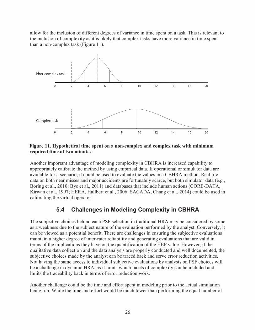
26

allow for the inclusion of different degrees of variance in time spent on a task. This is relevant to the inclusion of complexity as it is likely that complex tasks have more variance in time spent than a non-complex task (Figure 11).

Another important advantage of modeling complexity in CBHRA is increased capability to appropriately calibrate the method by using empirical data. If operational or simulator data are available for a scenario, it could be used to evaluate the values in a CBHRA method. Real life data on both near misses and major accidents are fortunately scarce, but both simulator data (e.g.,Boring et al., 2010; Bye et al., 2011) and databases that include human actions (CORE-DATA, Kirwan et al., 1997; HERA, Hallbert et al., 2006; SACADA, Chang et al., 2014) could be used in calibrating the virtual operator.

5.4 Challenges in Modeling Complexity in CBHRA

The subjective choices behind each PSF selection in traditional HRA may be considered by someas a weakness due to the subject nature of the evaluation performed by the analyst. Conversely, itcan be viewed as a potential benefit. There are challenges in ensuring the subjective evaluations maintain a higher degree of inter-rater reliability and generating evaluations that are valid in terms of the implications they have on the quantification of the HEP value. However, if the qualitative data collection and the data analysis are properly conducted and well documented, the subjective choices made by the analyst can be traced back and serve error reduction activities.Not having the same access to individual subjective evaluations by analysts on PSF choices will be a challenge in dynamic HRA, as it limits which facets of complexity can be included and limits the traceability back in terms of error reduction work.

Another challenge could be the time and effort spent in modeling prior to the actual simulation being run. While the time and effort would be much lower than performing the equal number of

Figure 11. Hypothetical time spent on a non-complex and complex task with minimum required time of two minutes.

Non-complex task

0

Complex task

4 6 8 10 12 14 16 20

0 4 6 8 10 12 14 16 20

27

traditional static HRAs, it would also likely be much higher than performing a single traditional static HRA.

A decision that has to be made in a CBHRA method is at what level to quantify, which will also influence depth in which the scenario is modeled. This has varied in traditional static HRA methods from those that quantify at the level of a button push (e.g., THERP, Swain & Guttmann,1983) to those that describe generic task types at a much higher level (e.g. HEART, Williams,1988 and 1992). Finding the appropriate level will be a challenge, but as CBHRA can use the quantifications to determine the path forwards from the task, it seems likely that the quantifications would be done at a low (e.g., subtask) level (Boring & Rasmussen 2016). Care must be made in any adaption from an HRA method that is capable of being applied at multiple levels of quantification. In fact, the level of quantification must also be matched with a compatible level of analysis contained within the PRA based plant model. In particular, the timelines for plant evolutions may somewhat dictate the appropriate resolution for the HRA quantification in order to allow both to run in sync during the simulation. For additional detail on quantification granularity, see Rasmussen and Laumann (2016).

5.5 Suggested Solution

The suggested solution of how complexity could be included in CBHRA models is through two types of inputs and two types of outputs. The inputs are:

1. The autopopulated aspects where the input is automatically gathered from the simulation, and

2. The prepopulated aspects that are based on how the task is categorized when the scenario is modeled.

The outputs are:

1. Path choice, with paths leading to success (with varying degrees of efficiency) and failure, and

2. Time spent on the task.

Both of these outputs would contribute to the HEP, but in a less direct way than in traditional static HRA. Including time spent on the task would also allow varying degrees of variance in time spent on tasks with varying degrees of complexity.

5.5.1 Autopopulation

The first form of “autopopulated input” is information that is automatically gathered from the details already present in the simulation computation. This input would perhaps be the preferred form of input, as it would require no additional efforts while building the scenario model.Examples of automatically gathered inputs for complexity include (with the corresponding complexity factors in parentheses):

Total size of the task or scenario (size complexity)

28

Number of success criteria (goal complexity)Number of alternative paths to the goal(s) (goal complexity)Number of steps conducted (step complexity)Number of tasks per time (temporal complexity)Time spent on task (temporal complexity)Time in scenarioDistance from basic event (structure complexity)“Errors” made so far (structure complexity)Current function of safety systems (structure complexity)Current function of general plant systems (structure complexity).

5.5.2 Prepopulation

Even though a CBHRA would not use an analyst to evaluate a task or scenario in the same way as a traditional static HRA, there will have to be some sort of categorization during the process of building the scenario model. The choices made in the categorization could be used as prepopulated inputs to complexity. The suggested prepopulated inputs are (with the corresponding complexity factors in parentheses):

Number of information cues the operator uses in this task (size complexity)Would this task be perceived as logical by the operators (compared to normal operations or other accident situations; structure complexity)Is the task influenced by factors outside of the operators control (dynamic complexity)Is the task connected to other tasks (connection complexity)Is the task connected to other parts of the plant or installation (connection complexity)Number of procedures used by the operator (procedure complexity)Number of page shifts done by the operator (procedure complexity)Ranking of the procedures (procedure complexity)Number of operators involved (interaction complexity)Number of HMI elements used (HMI complexity)HMI quality (HMI complexity)

Does the task rely on operator knowledge (knowledge complexity).

Figure 12. Quantification approach in traditional static HRA.

Qualitativedata

collection

Decisionsmade by

HRA analyst- Task type- PSF(s)- PSF levels

HumanError

Probability

29

5.5.3 Comparison

As mentioned, quantification will be fundamentally different between traditional static HRA (Figure 12) and CBHRA (Figure 13). The largest difference will be that the decisions made by ahuman reliability analyst in traditional static HRA will be modeled by a virtual operator in CBHRA. The decisions of the virtual operator will, however, be influenced by many of the same aspects as shape the traditional analysis. Before a scenario is simulated, potential tasks will have to be modeled, and this modeling will contain categorization elements that are similar to the task type and PSF choices that are made in traditional static HRA.

5.6 General Form of Complexity Modeling

Task complexity is an integral part of assessing the human component in a power plant. Task complexity has a direct influence on human performance in terms of time spent on a task and likelihood of success making it one of the most—if not the most—important factors to include in an assessment of human reliability. Evidence of the importance of task complexity can be seen in the fact that it has been included in almost all HRA methods (Rasmussen et al., 2015). A review (Boring, 2010) of analyses conducted using the SPAR-H method (Gertman et al., 2005) found that complexity was highly correlated with many other PSFs (see Table 3). As such, it is a reasonable PSF to model for its significant overall risk contribution in HRA. Additionally, while some PSFs are largely determined by internal factors, task complexity is largely driven by external factors, making it an ideal candidate for autopopulation in a dynamic model.

The complexity value is calculated through a numerical value association with each factor, prepopulated as part of the modeling multiplied with a weight. The associated weights are in

Figure 13. Suggested quantification approach in CBHRA.

Qualitativedata

collection

-0-Prepopulated

throughcategorization

Autopopulatedfrom the simulated

scenario

4444

Decisionsmade byvirtual

operator

Time spenton task

Pathchoice

30

equation (6) and (7) as a preassigned value determining the effect of each of the complexity factors. The use of weights allows for easy adjustments of the method.

Table 3. Spearman rank-order correlations between complexity and other PSFs in SPAR-H(adapted from Boring, 2010).

SPAR-H PSFs Diagnosis Complexity Action ComplexityAvailable Time -0.02 0.38*Stress/Stressors 0.15* 0.35*

Experience/Training 0.21* 0.32*Procedures 0.25* 0.12*

Ergonomics/HMI -0.05 0.08*Fitness for Duty -0.03 0.22*Work Processes 0.24* 0.16*

* Marked correlations are significant at p < 0.05

= × (6)

= + + + + (7)

where CF is the Complexity Factor and W is the Weight associated with the complexity factor.

The complexity factors can be categorized by plant parameters (such as temperature), task characteristics (such as procedures), and influences from other tasks (simultaneous tasks or tasks in near temporal proximity). The plant parameters and influences from other tasks will largely be autopopulated, while the task characteristics will be prepopulated as part of the task modeling.

= + +

(8)

Note that some PSFs like complexity may need to incorporate additional equations to account for lag and linger (Boring, 2015). Lag is a delay in the onset of the influence of that factor, while linger is an effect that continues even after the influences on that PSF cease. Additionally, PSFs may contain memory and decay.

Memory (a.k.a., history or hysteresis), which is related to lag and linger, means that the PSF remains anchored in its previous states, preventing dramatic surges in the face of sudden plant upsets or sudden dropouts in the absence of direct influences on the PSF. A memory of previous states reflects the pace of physiological changes in many cases, barring a sudden onset threat stress (e.g., fight or flight) that dramatically overrides existing physical and mental states. Memory is treated mathematically as a cumulative moving average and serves to smooth the PSF to sudden changes.Decay is a type of diminution of the effect of the PSF. In the absence of fresh drivers on its performance, a PSF should return to the nominal state over time. For example,

31

elevated stress caused by a plant upset will settle to a normal level after cessation of the event. There is significant linger in a PSF like stress; it does not simply abate when the source of the stress is removed. However, stress will not continue indefinitely, and it will eventually fade to a non-stress state. Thus, a decay function may be built into the basic function of the PSF to afford the gradual return to a predefined nominal state. Note that decay operates counter to linger—decay accelerates change to the PSF, while linger slows it.

These four dynamic PSF functions are summarized in Table 4. In Table 4, let PSF(t) be the shape function at time t. Assume events occur at times , = 1, … , . Lag and linger together are basically a continuity statement that can be combined into the following equation:

( ) = lim ( ) (9)

Table 4. Dynamic functions that may affect the general calculation of the PSF.

Dynamic PSF Function Effect on PSF Notation

lag A PSF will be slow to change at the outset of a new effect

( ) = lim ( )

lingerA PSF will be slow to change

at the termination of an existing effect

( ) = lim ( )

memory

General form of lag and linger, denoting that the effect

of the current PSF is a function of preceding values

for that PSF

( ) = ( )

decay A PSF will settle to its original state over time ( ) = (0)

32


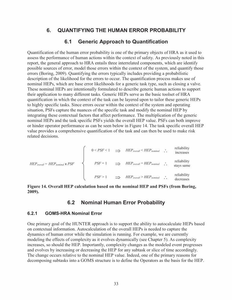
33

6. QUANTIFYING THE HUMAN ERROR PROBABILITY

6.1 Generic Approach to Quantification

Quantification of the human error probability is one of the primary objects of HRA as it used toassess the performance of human actions within the context of safety. As previously noted in this report, the general approach to HRA entails three interrelated components, which are identify possible sources of error, model those errors within the context of the system, and quantify those errors (Boring, 2009). Quantifying the errors typically includes providing a probabilistic description of the likelihood for the errors to occur. The quantification process makes use of nominal HEPs, which are base error likelihoods for a generic task type, such as closing a valve. These nominal HEPs are intentionally formulated to describe generic human actions to support their application to many different tasks. Generic HEPs serve as the basic toolset of HRA quantification in which the context of the task can be layered upon to tailor these generic HEPs to highly specific tasks. Since errors occur within the context of the system and operating situation, PSFs capture the nuances of the specific task and modify the nominal HEP by integrating these contextual factors that affect performance. The multiplication of the generic nominal HEPs and the task specific PSFs yields the overall HEP value. PSFs can both improve or hinder operator performance as can be seen below in Figure 14. The task specific overall HEP value provides a comprehensive quantification of the task and can then be used to make risk related decisions.

HEPoverall = HEPnominal x PSF

0 < PSF < 1 HEPoverall < HEPnominalreliabilityincreases

PSF = 1 HEPoverall = HEPnominalreliabilitystays same

PSF > 1 HEPoverall > HEPnominalreliabilitydecreases

Figure 14. Overall HEP calculation based on the nominal HEP and PSFs (from Boring, 2009).

6.2 Nominal Human Error Probability

6.2.1 GOMS-HRA Nominal Error

One primary goal of the HUNTER approach is to support the ability to autocalculate HEPs based on contextual information. Autocalculation of the overall HEPs is needed to capture the dynamics of human error while the simulation is running. For example, we are currently modeling the effects of complexity as it evolves dynamically (see Chapter 5). As complexity increases, so should the HEP. Importantly, complexity changes as the modeled event progresses and evolves by increasing or decreasing the HEP for any subtask or slice of time accordingly. The change occurs relative to the nominal HEP value. Indeed, one of the primary reasons for decomposing subtasks into a GOMS structure is to define the Operators as the basis for the HEP.

{

34

These Operators correspond to nominal HEP values, which can be modified by PSFs like complexity.

A reasonable starting point for quantifying the GOMS-HRA Operators is the original HRA method, THERP (Swain and Guttmann, 1983). THERP uses a template matching approach in which the analyst matches the current subtask being analyzed to similar, predefined subtasks provided in THERP lookup tables. Because THERP, unlike most other HRA methods, is subtask based, it aligns to the level of analysis required for quantifying the GOMS-HRA Operators. Table 5 provides an approximation of the nominal HEPs based on THERP values. The THERP lookup tables do not clearly delineate Action (A) and Selection (S), nor Checking (C) from Retrieval (R). In many cases, the GOMS-HRA Operators are more generic than the THERP lookup tables. As such, these values should be interpreted strictly as preliminary.

Written or implied procedural steps form the subtasks modeled in dynamic HRA. Although the degree of strict procedural adherence by nuclear power plant crews may be a matter for some debate (Forester et al., 2014), the procedures serve as mileposts for crew actions. Furthermore, for modeling purposes, the procedure steps serve to document the solution path, which is advantageous to represent crew actions within the modeling simulation. Thus, in order to model crew behavior dynamically, procedure steps are coded into the dynamic model. The value of GOMS-HRA is that by coding each step as an Operator, it is possible to imbue the model with additional information that makes HRA possible. Each Operator classifies the type of action being performed, which:

Defines the Operator state in terms of interactions with the plant in the overall dynamic model (e.g., by knowing a subtask is an Action, the coding specifies that the crew member will manipulate something at the plant, which can prompt the plant model to update itself or cause a new dynamic event tree),Specifies a time range for that action,Identifies possible error counterparts via SHERPA to successful task outcomes, andProvides a nominal HEP that may be used as the starting point in computing the dynamic HEP based on contextual factors for that subtask.

In short, Operator coding with GOMS-HRA becomes the skeleton to which other model elements are affixed. GOM-HRA nominal HEPs are listed in Table 5.

6.2.2 SPAR-H Nominal Error

SPAR-H was developed to simplify the complicated quantification process found in its predecessor, THERP. Therefore, SPAR-H uses a dichotic taxonomy to assign tasks to either a diagnosis or action type to simplify the quantification process. Action task types consist of procedurally based actions, such as manipulating controls to position a component’s setpoint or change the state of the component. Examples of actions include adjusting the position of a valve or starting a pump. Diagnosis task types entail a cognitive element in which courses of action are planned and strategies to control the plant are formulated. Examples of diagnosis include determining the cause of an alarm or the unexpected value displayed by an indicator. SPAR-H

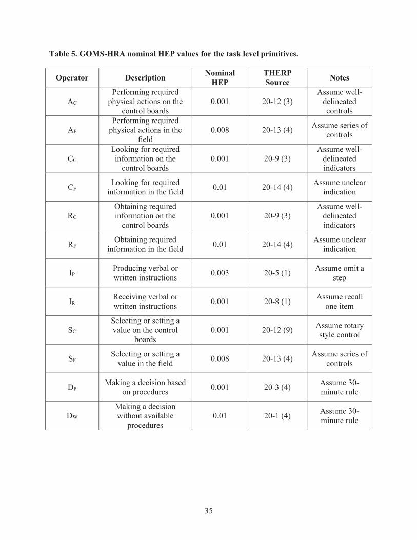
35

Table 5. GOMS-HRA nominal HEP values for the task level primitives.

Operator Description Nominal HEP

THERP Source Notes

AC

Performing required physical actions on the

control boards0.001 20-12 (3)

Assume well-delineated controls

AF

Performing required physical actions in the

field0.008 20-13 (4) Assume series of

controls

CC

Looking for required information on the


Assume well-delineated indicators

CFLooking for required

information in the field 0.01 20-14 (4) Assume unclear indication

RC

Obtaining required information on the


Assume well-delineated indicators

RFObtaining required

information in the field 0.01 20-14 (4) Assume unclear indication

IPProducing verbal or written instructions 0.003 20-5 (1) Assume omit a

step

IRReceiving verbal or written instructions 0.001 20-8 (1) Assume recall

one item

SC

Selecting or setting a value on the control

boards0.001 20-12 (9) Assume rotary

style control

SFSelecting or setting a

value in the field 0.008 20-13 (4) Assume series of controls

DPMaking a decision based

on procedures 0.001 20-3 (4) Assume 30-minute rule

DW

Making a decision without available

procedures0.01 20-1 (4) Assume 30-

minute rule

36

Table 6. SPAR-H nominal HEP values for the task level primitives.

Operator Description Diagnosis/ Action

SPAR-HNominal HEP Notes

AC

Performing required physical actions on the

control boardsAction 0.001 Manual action on

control boards

AF

Performing required physical actions in the

fieldAction 0.001 Manual local

action in the field

CC

Looking for required information on the

control boardsAction 0.001

Manual scan of boards for

information

CFLooking for required

information in the fieldDiagnosis +

Action 0.011 Manual local scan for information1

RC

Obtaining required information on the

control boardsAction 0.001 Manual retrieval

from boards

RFObtaining required

information in the fieldDiagnosis +

Action 0.011 Manual local retrieval1

IPProducing verbal or written instructions Diagnosis 0.001 Cognition/language

production

IRReceiving verbal or written instructions Diagnosis 0.001 Cognition/language

understanding

SC

Selecting or setting a value on the control

boards

Diagnosis + Action 0.011

Both thinking about value and

manually setting it

SFSelecting or setting a

value in the fieldDiagnosis +

Action 0.011Both thinking

about value and manually setting it

DPMaking a decision based

on procedures Diagnosis 0.001Reading procedure

and deciding course of action

DW

Making a decision without available

procedures

Diagnosis + Action 0.011

Likely to require carrying out

selected action2

1 It is assumed the field activities require greater cognitive engagement due to the balance of plant layout complexity. 2 It is assumed that such non-proceduralized activities will require manual actions to be carried out as part of the decision-making process. Otherwise, this is purely a Diagnosis task and would have a nominal HEP equal to 0.001.

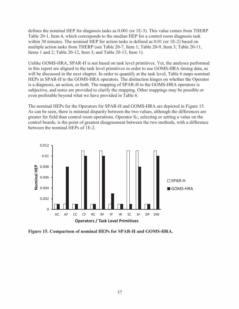
37

defines the nominal HEP for diagnosis tasks as 0.001 (or 1E-3). This value comes from THERP Table 20-1, Item 4, which corresponds to the median HEP for a control room diagnosis task within 30 minutes. The nominal HEP for action tasks is defined as 0.01 (or 1E-2) based on multiple action tasks from THERP (see Table 20-7, Item 1; Table 20-9, Item 3; Table 20-11,Items 1 and 2; Table 20-12, Item 3; and Table 20-13, Item 1).

Unlike GOMS-HRA, SPAR-H is not based on task level primitives. Yet, the analyses performed in this report are aligned to the task level primitives in order to use GOMS-HRA timing data, as will be discussed in the next chapter. In order to quantify at the task level, Table 6 maps nominal HEPs in SPAR-H to the GOMS-HRA operators. The distinction hinges on whether the Operator is a diagnosis, an action, or both. The mapping of SPAR-H to the GOMS-HRA operators is subjective, and notes are provided to clarify the mapping. Other mappings may be possible or even preferable beyond what we have provided in Table 6.

The nominal HEPs for the Operators for SPAR-H and GOMS-HRA are depicted in Figure 15.As can be seen, there is minimal disparity between the two values, although the differences are greater for field than control room operations. Operator SC, selecting or setting a value on the control boards, is the point of greatest disagreement between the two methods, with a difference between the nominal HEPs of 1E-2.

Figure 15. Comparison of nominal HEPs for SPAR-H and GOMS-HRA.

0

0.002

0.004

0.006

0.008

0.01

0.012

AC AF CC CF RC RF IP IR SC SF DP DW

Nom

inal

HEP

Operators / Task Level Primitives

SPAR-H

GOMS-HRA

HI II HI1

38


39

7. SIMULATION CASE STUDY: STATION BLACKOUT

7.1 Station Blackout Background

Typically, commercial nuclear power plants make use of external alternating current (AC) electrical power sources during normal operations while at power and during shutdown operations. Even if the reactor is not at criticality, the residual heat removal systems require AC power to disperse heat generated by the nuclear core. Loss of offsite power (LOOP) events refer to the situations in which the external AC electrical power source for the plant are rendered unavailable. LOOP events are categorized based on their initiating cause or location, which include plant centered, switchyard centered, grid related, and weather related (Eide et al., 2005). Plant centered LOOP events occur anywhere within the plant up to the auxiliary or station transformers. The appropriate response for plant centered LOOP events entails restoration of offsite power to the safety buses. Switchyard centered LOOP events occur with the switchyard and up to and including the output bus bar, and requires coordinated efforts between the plant and switchyard personnel to restore offsite power. Weather-related LOOP events can occur both within the plant or at the switchyard, but the defining characteristic is the weather causation to initiate the event (and these events may be somewhat long-lasting). Lastly, the grid-related LOOP event occurs somewhere within the external grid, which is particularly challenging because the power restoration requires coordination between the plant and external entities controlling the grid.

During a LOOP event, emergency diesel generators (DGs) start and run to provide AC electrical power until the offsite power can be restored. A station blackout refers to a particular type of LOOP event in which the emergency diesel generators also fail and the plant no longer has any access to AC electrical power. During station blackout events, the plant relies on systems that do not require AC electrical power, such as turbine-driven pumps used to circulate primary reactor coolant in order to support the residual heat removal efforts and maintain acceptable nuclear core temperatures. These systems have less capacity to remove the residual heat and ultimately will result in core damage if power is not restored within a sufficient timeframe. As a result of the significant threats posed by LOOP events and in particular station blackout LOOP events, it is important to analyze and model the risk associated with the event in order to formulate an optimal response strategy and provide guidance on the bounds in which the plant can safely operate to mitigate any detrimental effects.

7.2 Simplified Plant System

A PWR simplified model has been set up based on the parameters specified in the OECD main steam line break (MSLB) benchmark problem (Nuclear Energy Agency, 1999). The reference design for the OECD MSLB benchmark problem is derived from the reactor geometry and operational data of the Three Mile Island Unit 1 (TMI-1) Nuclear Power Plant, which is a 2772 MW two loop pressurized water reactor (see the system scheme shown in Figure 16).

40

Figure 16. Scheme of the TMI PWR benchmark (from Nuclear Energy Agency, 1999).

In order to simulate an SBO initiating event we need to consider also the following electrical systems (see Figure 17):

Primary power grid line 500 KV (connected to the 500 switchyard)Auxiliary power grid line 161 KV (connected to the 161 switchyard)Set of 2 diesel generators (DGs), DG1 and DG2, and associated emergency busesElectrical buses: 4160 V (step down voltage from the power grid and voltage of the electric converter connected to the DGs) and 480 V for actual reactor components (e.g., reactor cooling system)Direct current (DC) system which provides power to instrumentation and control components of the plant. It consists of these two sub-systems:

o Battery charger and AC/DC converter if AC power is availableo DC batteries: in case AC power is not available.

Loop B

Heat exchanger B

Pump B

Hot core channel

Downcomer B

Average core channel

Pressurizer

Loop A

Branch

Pump A

Upper Plenum

Bypass flow

Downcomer A

Lower Plenum

Cold core channel

Heat exchanger A

41

Figure 17. Scheme of the electrical system of the PWR model (from Nuclear Energy Agency, 1999).

7.3 Station Blackout Scenario

The specific station blackout event modeled in this simulation represents a prototypical station blackout event. Detailed procedure steps and substeps used in the model to quantify the HEP and completion times can be seen later in this chapter in Table 16. After the initial LOOP event, a reactor trip triggers, which prompts the operators to enter into an emergency operating procedure, i.e., standard post trip actions. During the post trip actions procedure, the operators perform a number of plant diagnostic steps to ensure the plant is operating within safety envelopes. First they confirm the reactor successfully tripped by verifying a downward trend in reactor power. The operators then confirm the turbine has tripped and the main output breakers have opened. At this point operators’ efforts turn toward confirming the safety systems are functioning properly, which includes assessing that the reactor coolant system inventory is sufficient, ensuring at least one recirculating coolant pump is in operation, and residual heat removal is capable of dissipating heat from the recirculated coolant. Lastly, the operators check the integrity of containment by verifying no radiation alarms are present and assessing containment pressure and temperatures. A detailed timeline of the scenario follows below (also see Figure 18):

500 KV

500 KVSwitchyard

4160 V

161 KV

161 KVSwitchyard

H T11A

.--1 T11D

480 V—0— ECCS

1 4800V

1 4800V

480 V—0—

Battery —0—charger

480 V—0-

48,::$ V 1

4800 V 1

480 V

..,___L_ 250 VDC- I I—

DC Battery

4160 V

T12

HA

T12B 1--.

T12C H

T12D

1--.

1--0— Instrumentationand control

„1 (1 (I.. c 4160 V

\ Emergency buses

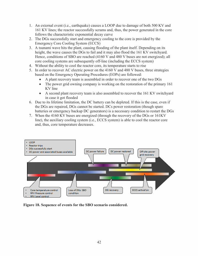
42

1. An external event (i.e., earthquake) causes a LOOP due to damage of both 500 KV and 161 KV lines; the reactor successfully scrams and, thus, the power generated in the core follows the characteristic exponential decay curve

2. The DGs successfully start and emergency cooling to the core is provided by the Emergency Core Cooling System (ECCS)

3. A tsunami wave hits the plant, causing flooding of the plant itself. Depending on its height, the wave causes the DGs to fail and it may also flood the 161 KV switchyard. Hence, conditions of SBO are reached (4160 V and 480 V buses are not energized); all core cooling systems are subsequently off-line (including the ECCS system)

4. Without the ability to cool the reactor core, its temperature starts to rise5. In order to recover AC electric power on the 4160 V and 480 V buses, three strategies

based on the Emergency Operating Procedures (EOPs) are followed:A plant recovery team is assembled in order to recover one of the two DGs The power grid owning company is working on the restoration of the primary 161 KV line A second plant recovery team is also assembled to recover the 161 KV switchyard in case it got flooded

6. Due to its lifetime limitation, the DC battery can be depleted. If this is the case, even if the DGs are repaired, DGs cannot be started. DCs power restoration (though spare batteries or emergency backup DC generators) is a necessary condition to restart the DGs

7. When the 4160 KV buses are energized (through the recovery of the DGs or 161KV line), the auxiliary cooling system (i.e., ECCS system) is able to cool the reactor core and, thus, core temperature decreases.

Figure 18. Sequence of events for the SBO scenario considered.

• LOOP

• Reactor trips

• DGs successfully start• DC power and associated buses available

-1• Core temperature control Loss of DGs: SBO• RPV Pressure control condition

RPV Level control ..

DC power failure

.

,

. DC power restored

DG recovery

c N

Off-site powergrid recovery

43

7.4 Stochastic Parameters

For the scope of this report, the following parameters are uncertain:

1. _ : recovery time of the DGs2. _ : recovery time of the 161 KV power grid3. _ : failure time of the batteries (DC system) due to depletion4. _ : recovery time of the batteries (DC system).

For each of these parameters we will find the appropriate probability distribution function in order to evaluate core damage probability . Core damage is reached when max clad temperature in the core reaches its failure temperature (2200° F).

To analyze the risk associated with a station blackout, the GOMS-HRA method was applied. The GOMS-HRA method entails decomposing procedure steps into task primitives, which are then used to calculate completion time and HEP values for each procedure step. The completion time and HEP values were then input to the RAVEN model to simulate human error events and their outcomes in relation to plant thermo-hydraulics.

7.5 RAVEN Implementation

The reactor vessel model consists of the Down-comers, the Lower Plenum, the Reactor Core Model and the Upper Plenum. Three Core-Channels (components with a flow channel and a heating structure) were used to describe the reactor core. Each Core-Channel is representative of a region of the core (from one to thousands of real cooling channels and fuel rods).

In this analysis, the core model consists of three parallel Core-Channels (hot, medium and cold) and one bypass flow channel. Respectively they represent the inner and hottest zone, the mid,and the outer and colder zone of the core. The Lower Plenum and Upper Plenum are modeled with Branch models.

There are two primary loops in this model—Loop A and Loop B. Each loop consists of the Hot Leg, a Heat Exchanger and its secondary side pipes, the Cold Leg and a primary Pump. A Pressurizer is attached to the Loop-A piping system to control the system pressure. Since a complex Pressurizer model has not been implemented yet in the current version of RELAP-7code, a Time Dependent Volume (pressure boundary conditions) has been used instead.

Figure 19 shows the core layout of the pressurized water reactor (PWR) model. The core height is 3.6576 m. The reactor consists of 177 fuel assemblies subdivided in 3 zones. The 45 assemblies in zone 1 are represented by the hot core channel, and the 60 assemblies in zone 2 and 72 assemblies in zone 3 are respectively represented by the average core channel and the cold core channel. The fuel assembly geometry data are taken from U.S. Nuclear RegulatoryCommission reference data (U.S. NRC, 1975). The reactor is assumed to be at end of cycle (EOC), 650 EFPD (24.58 GWd/MHMt average core exposure), with a boron concentration of 5 ppm, and Xe and Sm at the equilibrium. The 3-D core neutronics calculation results for the hot full power condition are presented in Todorova, Ivanov, and Taylor (2003).

44

Figure 19. Screenshot of the PWR model of RELAP-7 using PEACOCK.

Figure 20. Core zone correspondence (left) and assembly relative power (right).

Figure 20 shows the relative assembly radial power distribution for a quarter of the core. Using the values presented in Figure 20, the power distribution fraction and power density for each Core-Channel is calculated and shown in the Table 7. The power density is used as input to the RELAP-7 model to calculate the heat source.

Reflector

=MEM=NM MIME Mr

EMI =MENEM= MNNM =MEM= MN MNMENEM MME

EN NEE MENNE MEN EEl EN NE MENNEN NE N■NN NN =EMMEN NN N■NN NN EMMEN NN N■NN NN =MENNE NN EN N■EN NN MENEM= NN E

■N NEN MENEM NEN NNEN NNE N

NE EN MENNEN. NE ENMENNEENEM

EINE MENEM NEENEMEENE

0,918 1.253 1.057 1.285 1,031 1.248 0.805 0.439

1,253 1.023 1.270 1.051 1.278 1.048 1.124 0.496

1.057 L270 1.039 L278 1.022 1.254 1.051 0.476

1.285 1.053 1.278 1.048 1.273 0.952 0.767

1.031 1.282 L022 1.271 1.035 1.093 0_580

1.248 1.043 1.254 0,952 1.093 0.740

0.805 1.121 1.051 0.767 0.580

0.439 0.493 0.475

45

Table 7. Power distribution factor for representative channels and average pellet power.

Core Channel Power Distribution Factor

Average fuel pellet power density (W/m3)

Hot 0.3337 3.90 108

Average 0.3699 3.24 108

Cold 0.2964 2.17 108

7.5.1 Component Modeling

Several control logic related models have been included into the RAVEN/RELAP-7 simulations; these are:

Pump coast downDecay heatDGsPower Grid (PG)Battery system4160 V bus.

All these components have been defined in the RAVEN/RELAP-7 input file and both links and dependencies among them are defined in the RAVEN control logic part. Such features allow us to perform a component-centric modeling of the scheme.

Examples of RAVEN components defined in the RAVEN/RELAP-7 input file include:

Pump coast down: this block of the input files defines how the pumps in the primary loop decrease their speed in an exponential fashion. Such components are used in the control logic part of RAVEN to act on the head of the RELAP-7 pumps (controlled variable) at a specific time instant (monitored variable) as follows:

controlled.Head_Pump = tools.PumpCoastDown.compute(monitored.time)

Power grid (PG): this block defines a binary variable (i.e., on/off type) for the power grid. Power grid status is set to 0.0 at the beginning of the transient and then set to 1.0 when time reaches the power grid recovery time.Batteries: These are defined similarly to the power grid input block. The main difference is that the battery life can be computed and updated at each time step.

7.5.2 RAVEN Control Logic

The plant control logic has been coded in PYTHON according to RAVEN simulation controller schema. Given the sampled parameters: _ , _ , _ and _ , the control logic pseudo codes for DG, PG, and batteries are shown below (see Pseudo code 1, 2 and 3).

46

The basic idea is that in order to recover AC power either the DGs or the PG need to be recovered (see Table 8. Pseudo code 1). Regarding the DG recovery (see Table 9. Pseudo code 2), even if the DGs are actually fixed, they cannot be started without DC power available (i.e., batteries).

Table 8. Pseudo code 1: Battery system control logic

# Battery control logicif time <= batt_FailTime

battStatus = Trueelse if time > batt_FailTime and time <= (batt_FailTime + batt_RecTime)and (not ACStatus)

auxiliary.battStatus = Falseelse if time > (batt_FailTime + batt_RecTime) or ACStatus

auxiliary.battStatus = True

Table 9. Pseudo code 2: DG and PG control logic

# DG control logicif time >= (DG_failTime + DG_recoveryTime) and battStatusDGStatus = Trueelse if time <= (DG_failTime)DGStatus = TrueelseDGStatus = False

# PG control logicif time >= PG_recoveryTime

PGStatus = Trueelse

PGStatus = False

Table 10. Pseudo code 3: AC power status control logic

# AC statusif PGStatus or DGStatus

ACStatus = Trueelse

ACStatus = False

7.5.3 Transient Example

An example of a transient simulated using RAVEN/RELAP-7 is shown in Figure 21. In order to reach a steady state condition, the simulation is being run for 500 seconds without any change in its internal parameters.

At = 500 , the external initiating event (i.e., earthquake) caused a LOOP event. The reactor successfully scrams, AC power is provided by the DGs and the ECCS keeps the reactor core cool.

At = 2000 , the tsunami induced flooding disables the DGs which were providing emergency AC power. Without AC power, the ECCS is disabled as well and the core temperature increases.

47

When AC power is recovered (through either DG or PG recovery) the ECCS capabilities are restored and core temperature starts to decrease.

Figure 21. Example of LOOP scenario followed by DGs failure using the RELAP-7 code.

For the PG recovery time _ we used as reference NUREG/CR-6890 vol.2 (data collection was performed between 1986 and 2004; Eide, Gentillon, Wierman, & Rasmuson, 2005). Given the four possible LOOP categories (i.e., plant centered, switchyard centered, grid related, or weather related), severe/extreme events (such as earthquake) are assumed to be similar to these events found in the weather category, which are typically long-term types of recoveries. This category is represented with a lognormal distribution (from NUREG/CR-6890) with = 0.793and = 1.982 (see Figure 22).

(a) (b)Figure 22. Plot of the pdfs of PG time recovery ( _ ) and DG time recovery ( _ ).

Regarding battery life (i.e., _ ), we chose to limit battery life between 4 and 6 hours using a triangular distribution (see Figure 23). In conclusion, Table 11 summarizes the distribution associated with each uncertainty parameter.

Steady statecalculation

Reactor scram

AC powerrecovery

AC power lost

48

(a) (b)Figure 23. Plot of the pdfs of battery life ( _ ) and battery recovery time ( _ ).

Table 11. Probability distribution functions for sets of uncertainty parameters.

Parameter Distribution

_ (h) Weibull (alpha = 0.745, beta = 6.14)

_ (h) Lognormal (mu = 0.793, sigma = 1.982)

_ (h) Triangular (4.0, 5.0, 6.0)

_ (h) Lognormal (mu = 0.75, sigma = 0.25)

7.6 GOMS-HRA Procedure Primitives

The station blackout scenario used to illustrate the GOMS-HRA method contains procedure steps containing specific verb terminology. Procedure writing guidelines suggest following the convention of consistently using a single verb to denote a particular action. Operators are trained to interpret the verb during the training so that each procedure step is clearly defined and intuitive for the operator to complete. We followed the standard conventions to define each verb used in each procedure step of the Post Trip Actions (PTA) and Station Blackout procedures (Procedure Professional Association, 2016; Jang et. al, 2010). Defining the verbs with standardized definitions enables the HRA task primitives to map onto each specific procedure step (see Table 12) and provide timing data. Each verb represents a single primitive or a series of combined primitives required to complete the procedure step. At each step in the procedure, the RAVEN model is provided with the appropriate timing and HEP data.

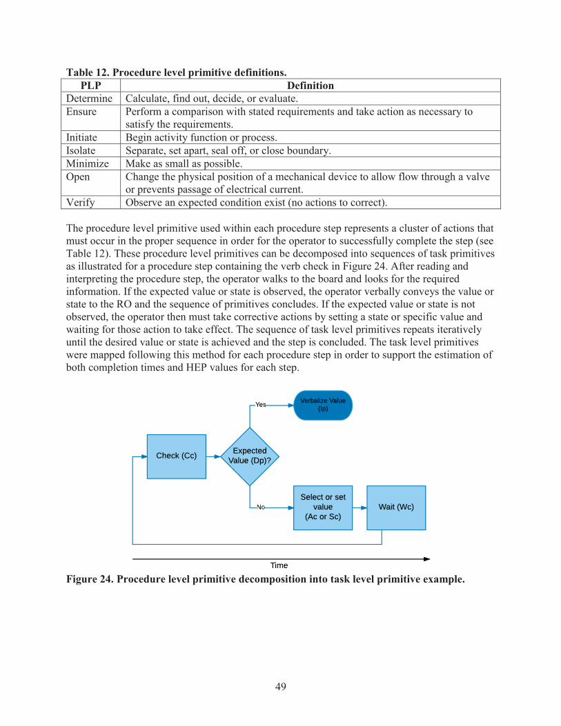
49

Table 12. Procedure level primitive definitions.PLP Definition

Determine Calculate, find out, decide, or evaluate.Ensure Perform a comparison with stated requirements and take action as necessary to

satisfy the requirements.Initiate Begin activity function or process.Isolate Separate, set apart, seal off, or close boundary.Minimize Make as small as possible.Open Change the physical position of a mechanical device to allow flow through a valve

or prevents passage of electrical current.Verify Observe an expected condition exist (no actions to correct).

The procedure level primitive used within each procedure step represents a cluster of actions that must occur in the proper sequence in order for the operator to successfully complete the step (see Table 12). These procedure level primitives can be decomposed into sequences of task primitives as illustrated for a procedure step containing the verb check in Figure 24. After reading and interpreting the procedure step, the operator walks to the board and looks for the required information. If the expected value or state is observed, the operator verbally conveys the value or state to the RO and the sequence of primitives concludes. If the expected value or state is not observed, the operator then must take corrective actions by setting a state or specific value and waiting for those action to take effect. The sequence of task level primitives repeats iteratively until the desired value or state is achieved and the step is concluded. The task level primitives were mapped following this method for each procedure step in order to support the estimation ofboth completion times and HEP values for each step.

Figure 24. Procedure level primitive decomposition into task level primitive example.

Check (Cc)

—Yes

ExpectedValue (Dp)?

Verbalize Value

010)

Select or setNo value

(Ac or Sc)Wait (Wc)

Time

50

Table 13. Generic procedure level primitive mapping to task level primitives.

Procedure Level Primitive Task Level Primitive Mapping NotesDetermine* CC or RC Information type dependentEnsure* CC or RC and/or AC and/or SC Information and control action

type dependentInitiate AC -Isolate AC -Minimize SC -Open AC -Verify* CC, RC Information type dependent*These procedure level primitives can be decomposed into multiple task level primitives as illustrated in Figure 24 depicting the check procedure primitive decomposed into DP, AC, SC,WC, and IP task level primitives.

Table 13 depicts the procedure level primitives identified in the simulation log data that wereused to decompose the procedure level primitives into task level primitives. The procedure level primitives are generically defined in this table since the object on which the procedure level primitive operates is not defined. The next step is categorizing the procedures based on procedure level primitives in preparation for decomposing these procedural level primitives into task level primitives.

7.6.1.1 Defining Nominal Timing Data and HEPs

In order to analyze a specific scenario, such as the station blackout event, and calculate the nominal HEP and task timing values, the procedure must be evaluated at the procedure level and then at the task level. The procedures included in this simulation are based on the post trip action and station blackout procedures from a nuclear utility. To protect the proprietary procedures, the procedure text cannot be publicly disseminated. Therefore the text for each procedure step has been redacted in Table 16.

Since the procedure steps cannot be shared in this report, an example procedure step in Table 14serves to provide an overview of how a step is mapped to the procedure level and task level primitive. For example, procedure step 2 of the post trip actions procedure contains two procedure level primitives, which are determine and verify. Determine is an abstract procedure level primitive that can be decomposed into three verify substeps. These substeps of procedure 2are mapped onto the task level primitive of verify, which corresponds to the task level primitive, CC, or looking for required information on the control boards.

Table 14. Example mapping of procedure step to procedure and task level primitives.

PTA 2 Determine maintenance of vital auxiliarics acceptance critcria arc mct: Determine'PTA 2 a Verify the main turbine is tripped Verify Cc

PTA 2 b Verify the main generator output breakers are opcn Vcrify Cc

51

To reiterate the process, two mappings are involved:

The plant procedures are classified in terms of procedure level primitivesThese procedure level primitives are comprised of task level primitives from GOMS-HRA.

Because there is a high degree of nuclear industry consensus on terminology in operating procedures, the procedure level primitives represent commonly and consistently deployed types of activities. It is therefore possible to create a universal mapping of GOMS-HRA task level primitives to the procedure level primitives. This universal mapping affords the opportunity for reuse of the building blocks in HUNTER across different analyses.

The procedures are an approximation of the actual series of events that would unfold during the scenario. Though this reduces some of the realism captured in the simulation, it was necessary due to the procedures’ proprietary nature. Furthermore, this is the first attempt at performing an integrative HRA model with dynamic HEPs and corresponding thermal-hydraulic computations,which was made possible by restricting the scope of the simulation to these two generic procedures. To illustrate this analysis further, station blackout procedure 5a stating “Ensure letdown is isolated” will be described at each stage of the analysis process (see Table 15). The procedure level primitive in this step is defined as the verb, Ensure. Ensure could be decomposed into different task level primitives, so the context of the procedure step, in this case letdown isolation, must be evaluated to determine which of the task level primitives are applicable. In this instance, the valve positions are a status indicator with a simple state control as opposed to a continuous numerical value setting. As a result, this procedure level primitive translates to the task level primitives of CC (look for required information on the control board) and AC (perform physical actions on the control board).

Table 15. SBO Step 5 showing mapping of Ensure procedure level primitive.

The procedure steps for the PTA and SBO procedures were mapped to procedure and task level primitives as shown in Table 16. Following the analysis of the procedures to map procedure level and task level primitives, timing data were estimated for each procedure step as derived from GOMS-HRA. Additionally, the procedure steps were aligned with the two primary events in which the LOOP occurs and the loos of diesel generators (LODG) and loss of battery (LOB) during the station blackout event (see Table 17).

SBO 5 - Minimize rector coolant system leakage Minimize' -SBO

5 a Ensure letdown is isolated EnsureCc

SBO Ac

SBO 5 b Ensurc reactor coolant pump controllcd bleedoff is isolated Ensure CcSBO 5 c Ensure reactor coolant system sampling is isolated Ensure Cc

52

Table 16. Post trip actions and station blackout procedures mapped to procedure and task level primitives.

1Procedure steps at a higher level of analysis than the task level primitives of GOMS-HRA. These steps were not included in the model, but rather the actions of these steps were captured within their respective substeps and these substeps were included in the model.

Procedure Step Substep Text PLP TLPPTA I Determine' -PTA I a Verify Rc

PTA l b Verify Rc

PTA I c Vcrify RcPTA 2 Determine' -PTA 2 a Verify Cc

PTA 2 b Verify Cc

PTA 2 c Verify Cc

PTA 3 - Determine' -

PTA 3 a Verify Rc

PTA 3 b Verify Rc

PTA 4 - Verify Rc

PTA 5 - Determine' -PTA 5 a Verify Cc

PTA 5 b Verify Rc

PTA 5 c Verify RcPTA 6 -

Procedure Text Not Publically Available

Determine' -

PTA 6 a Verify Rc

PTA t, b Verify Rc

PTA ( c Verify RcPTA - Determine' -PTA 7 a Verify Rc

PTA 7 b Verify Cc

PTA 7 c Verify CcPTA 8 - Determine' -PTA 8 a Verify Rc

PTA 8 b Vcrify RcPTA 9 - Determine' -PTA 9 a Verify Rc

PTA 9 b Verify Rc

SBO 3 - Open RcSBO 4 - Isolate' -

SBO4 a Ensure

Cc

SBO Ac

SBO4 b Ensure

Cc

SBO Ac

SBO4 c Ensure

Cc

SBO AcSBO 5 - Minimize' -

SBO5 a Ensurc

Cc

SBO Ac

SBO 5 b Ensure Cc

SBO 5 c Ensure Cc

SBO6 - Ensure

Rc

SBO Sc

SBO7 - Ensure

Rc

SBO Sc

SBO8 - Ensure

Cc

SBO Ac

SBO 9 - Initiate Ac

53

Table 17. Procedure steps and associated task level primitives mapped onto the main events of the modeled scenario and the estimated timing data.

7.7 Autocalculating the Complexity Performance Shaping Factor

7.7.1 SPAR-H Complexity

We have chosen to use the complexity framework from the SPAR-H method (Gertman et al., 2005) as the starting point of reference for both the range and distribution of the complexity value. In SPAR-H, the complexity PSF ranges from a minimum value of 0.1 to a maximum value of 5. These PSF values function as HEP multipliers, leading to an increase (up to 5 times

Procedure Failure Events TimeProcedure Step Substep TLP LOOP LODG LOB St h Expected 95th

PTA 1 - - 1 0 0 - -PTA I a Rc I 0 0 3.08 9.81 21.9PTA 1 b Rc I 0 0 3.08 9.81 21.9PTA 1 c Rc I 0 0 3.08 9.81 21.9PTA 2 - - 1 0 0 - - -PTA 2 a Cc 1 0 0 2.44 11.41 29.88PTA 2 b Cc I 0 0 2.44 11.41 29.88PTA 2 c Cc i 0 0 2.44 11.41 29.88PTA 3 - - i 0 0 - - -PTA 3 a Rc I 0 0 3.08 9.81 21.9PTA 3 b Rc I 0 0 3.08 9.81 21.9PTA 4 Rc I 0 0 3.08 9.81 21.9PTA 5 0 0 - - -PTA 5 a Cc I 0 0 2.44 11.41 29.88PTA 5 b Rc I 0 0 3.08 9.81 21.9PTA 5 c Rc I 0 0 3.08 9.81 21.9PTA 6 - - 0 0 - - -PTA 6 a Rc I 0 0 3.08 9.81 21.9PTA 6 b Rc i 0 0 3.08 9.81 21.9PTA 6 c Rc I 0 0 3.08 9.81 21.9PTA 7 - - I 0 0 - - -PTA 7 a Rc I 0 0 3.08 9.81 21.9PTA 7 b Cc I 0 0 2.44 11.41 29.88PTA 7 c Cc I 0 0 2.44 11.41 29.88PTA 8 - - I 0 0 - - -PTA 8 a Rc I 0 0 3.08 9.81 21.9PTA 8 I, Rc 1 0 0 3.08 9.81 21.9PTA 9 - 1 0 0 - - -PTA 9 Rc 1 0 0 3.08 9.81 21.9PTA 9 l• Rc I 0 0 3.08 9.81 21.9SBO 3 Rc I 1 0 3.08 9.81 21.9

SBO 4 - I I 0 - - -SBO

4Cc 1 1 0 2.44 11.41 29.88

SBO Ac 1 1 0 1.32 18.75 65.26SBO

4 bCc I 1 0 2.44 11.41 29.88

SBO Ac i 1 0 1.32 18.75 65.26

SBO4 c

Cc i 1 0 2.44 11.41 29.88SBO Ac 1 0 1.32 18.75 65.26SBO 5 - - 1 1 0 - - -SBO

5 aCc 1 1 0 2.44 11.41 29.88

SBO Ac I 1 0 1.32 18.75 65.26SBO 5 b Cc 1 1 0 2.44 11.41 29.88

SBO 5 c Cc I 1 0 2.44 11.41 29.88

SBO6 -

Rc 1 1 0 3.08 9.81 21.9

SBO Sc I 1 0 3.01 34.48 115.57

SBO7

Rc I 1 0 3.08 9.81 21.9

SBO Sc I 1 0 3.01 34.48 115.57SBO

8 _ Cc I 1 0 2.44 11.41 29.88SBO Ac I 1 0 1.32 18.75 65.26SBO 9 - Ac I 1 0 1.32 18.75 65.26

54

more) or decrease (up to 10 times less for the PSF of 0.1) in the likelihood of human error. In Table 18, Action and Diagnosis complexity from the SPAR-H worksheet are displayed along with their frequency data obtained from Boring et al. (2006).

PSF PSF Level Multiplier FrequencyComplexity:

DiagnosisHighly Complex 5 3Moderately Complex 2 30Nominal 1 500Obvious Diagnosis 0.1 Not ReportedInsufficient Information

1 2

Complexity: Action Highly Complex 5 3Moderately Complex 2 30Nominal 1 500Insufficient Information

1 2

Table 18. SPAR-H worksheet excerpt for the Complexity PSF level multipliers.

The complexity PSF was then fit with several distributions using a maximization likelihood estimate (MLE). For each distribution fit, an Akaike information criterion (AIC), Bayes information criterion (BIC), and log-likelihood was recorded along with the distribution parameters (see Table 19). AIC and BIC are relative measurements for the quality of statistical models for a given set of data. AIC and BIC provide a measurement for goodness of fit;however. Unlike the p-value common in inferential statistics, it does not provide a universal indication if the fit is bad; instead, it ranks the available fitted distributions. Using an MLE on the SPAR-H Complexity PSF level frequency data, well know statistical distributions were fit with the following results displayed in Table 19.

Distribution AIC BIC Log-Likelihood parameter 1 parameter 2Lognormal -1515.942 -1502.908 759.971 0.048 0.198Gamma 282.468 295.502 -139.234 18.099 16.783Normal 4428.581 4441.615 -2212.290 1.078 0.377Weibull 4668.917 4681.951 -2332.458 2.464 1.195Exponential 10756.785 10763.302 -5377.392 0.927 NAUniform NA NA NA 1 5Table 19. Fitting of distributions to SPAR-H frequency data from Boring et al. (2006)

The smallest AIC and/or BIC indicate the distribution that fits the best for complexity is Lognormal with mean-log of 0.048 and standard deviation-log of 0.198. Based upon these results, the distribution for complexity in the new dynamic method should retain a very similar shape. Based upon identified outputs from the simulation, data used to generate equation are in Table 20.

55

7.7.2 Calculating Complexity

We calculated complexity by two methods—linear and stochastic. The linear method simply reflects a traditional multiple regression equation based on a representative simulator run. In the linear form, the coefficients are fixed to a single value. In the stochastic form, the coefficients represent a range of values, thereby more accurately modeling uncertainty. The linear and stochastic forms of complexity are compared to each other later in the SBO simulations described in Section 7.9.

7.7.2.1 Linear Form of Complexity

A basic 20 task dataset was generated for illustrative purposes, which is displayed in Table 20.Complexity increases and decreases based on the situation the operator is facing. Loss of off-site power (LOOP), loss of diesel generator (LODG), and loss of battery (LOB) are all considered binary: 1 means there has been a loss, and 0 means the system is operating within normal parameters. Reactor temperature and reactor power level are both randomly sampled from RAVEN simulations of an SBO scenario.

Table 20. A 20-task breakdown of complexity for a station blackout event.

Task LOOP LODG LOB Reactor Temperature

Reactor Power Level

SME Complexity

Calculated Complexity

Normalized Complexity

1 0 0 0 566.69 100.00 1 -2.57 1.002 0 0 0 565.00 99.99 1 -2.56 1.003 0 0 0 568.69 100.00 1 -2.57 1.004 0 0 0 567.44 99.99 1 -2.57 1.005 1 0 0 540.28 3.15 3 4.40 2.776 1 0 0 539.92 2.95 3 4.40 2.777 1 0 0 539.49 2.79 3 4.40 2.778 1 0 0 561.59 2.38 3 4.39 2.769 1 0 0 538.57 2.48 3 4.41 2.77

10 1 0 0 538.55 2.63 3 4.41 2.7711 1 0 0 538.55 2.63 3 4.41 2.7712 1 0 0 538.55 2.63 3 4.41 2.7713 1 1 0 575.73 1.36 4 9.40 4.0314 1 1 0 624.89 1.29 4 9.35 4.0215 1 1 1 1775.04 0.75 5 13.21 5.0016 1 1 1 2092.49 0.66 5 12.89 4.9217 1 1 1 2257.35 0.60 5 12.73 4.8818 1 1 1 2374.40 0.54 5 12.61 4.8519 1 1 1 2407.60 0.00 5 12.59 4.8420 1 1 1 2400.87 0.51 5 12.59 4.84

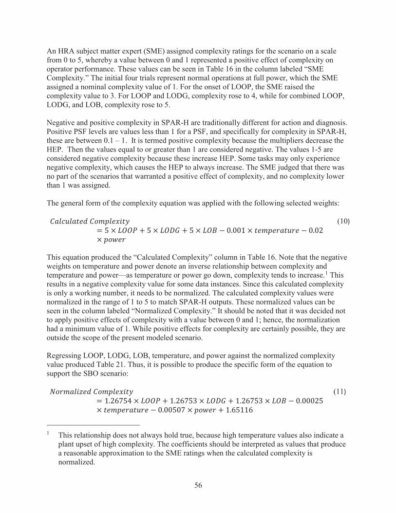
56

An HRA subject matter expert (SME) assigned complexity ratings for the scenario on a scale from 0 to 5, whereby a value between 0 and 1 represented a positive effect of complexity on operator performance. These values can be seen in Table 16 in the column labeled “SME Complexity.” The initial four trials represent normal operations at full power, which the SME assigned a nominal complexity value of 1. For the onset of LOOP, the SME raised the complexity value to 3. For LOOP and LODG, complexity rose to 4, while for combined LOOP, LODG, and LOB, complexity rose to 5.

Negative and positive complexity in SPAR-H are traditionally different for action and diagnosis. Positive PSF levels are values less than 1 for a PSF, and specifically for complexity in SPAR-H, these are between 0.1 – 1. It is termed positive complexity because the multipliers decrease the HEP. Then the values equal to or greater than 1 are considered negative. The values 1-5 are considered negative complexity because these increase HEP. Some tasks may only experience negative complexity, which causes the HEP to always increase. The SME judged that there was no part of the scenarios that warranted a positive effect of complexity, and no complexity lower than 1 was assigned.

The general form of the complexity equation was applied with the following selected weights:

= 5 × + 5 × + 5 × 0.001 × 0.02×

(10)

This equation produced the “Calculated Complexity” column in Table 16. Note that the negative weights on temperature and power denote an inverse relationship between complexity and temperature and power—as temperature or power go down, complexity tends to increase.1 This results in a negative complexity value for some data instances. Since this calculated complexity is only a working number, it needs to be normalized. The calculated complexity values were normalized in the range of 1 to 5 to match SPAR-H outputs. These normalized values can be seen in the column labeled “Normalized Complexity.” It should be noted that it was decided not to apply positive effects of complexity with a value between 0 and 1; hence, the normalization had a minimum value of 1. While positive effects for complexity are certainly possible, they are outside the scope of the present modeled scenario.

Regressing LOOP, LODG, LOB, temperature, and power against the normalized complexity value produced Table 21. Thus, it is possible to produce the specific form of the equation to support the SBO scenario:

= 1.26754 × + 1.26753 × + 1.26753 × 0.00025× 0.00507 × + 1.65116

(11)

1 This relationship does not always hold true, because high temperature values also indicate a plant upset of high complexity. The coefficients should be interpreted as values that produce a reasonable approximation to the SME ratings when the calculated complexity is normalized.

57

Table 21. Regression output with complexity as the dependent variable, based on the data from Table 20.

Weight t-Score p-levelIntercept 1.65116 1,148.73 0.001

LOOP 1.26754 909.87361 0.001LODG 1.26753 59,778.28 0.001LOB 1.26753 36,441.29 0.001

Temperature -0.00025 -11,070.97 0.001Power -0.00507 -354.14571 0.001

Note that complexity will vary depending on the exact simulation run. A sample set of complexity values is provided in Table 22. Also note that the normalized complexity value serves as the multiplier on nominal HEPs for each task level primitive as discussed in the next section.

7.7.2.2 Stochastic Form of Complexity

Creation of a model that accommodates the changing events occurring in a nuclear power plant to assess complexity was deemed desirable. The method for fitting this equation works with the distributions of the simulated variables with a 99% accuracy. The 1% of inaccurate complexity grades created by the equation was classified as such because they received a complexity score outside of the 0-5 range. The first step to creating this accurate equation is identifying the distributions which were associated with the SBO variables. These distributions are displayed in Table 23.

Then sampling from the defined distributions in Table 23 is matched to the procedural steps associated with SBO. These procedures have GOMS-HRA task level primitives. LOOP was assumed to have occurred within the first step triggering the SBO procedures. This is then followed by the LODG and finally the LOB. The order of loss events is assumed to remain constant; however, the step in which they fail is not the same procedure step for each iteration. In addition to the changing time of the loss events, temperature and reactor power level also fluctuate within a confined realm of uncertainty. Thus, the data displayed within Table 24 is one iteration of the simulation that is generated 5,000 times.

After each of the coefficients of the regression equation is retained, normal distributions are fit to the coefficient data. Additionally the distribution of the p-values associated with each coefficient and the intercept are recorded, and the majority of the observations were well below 0.05. As previously stated the data in Table 24 is created 5000 times. Each iteration has a regression equation fit to it. Table 25 contains a sample of 9 regression coefficients and intercepts from the data fitting.

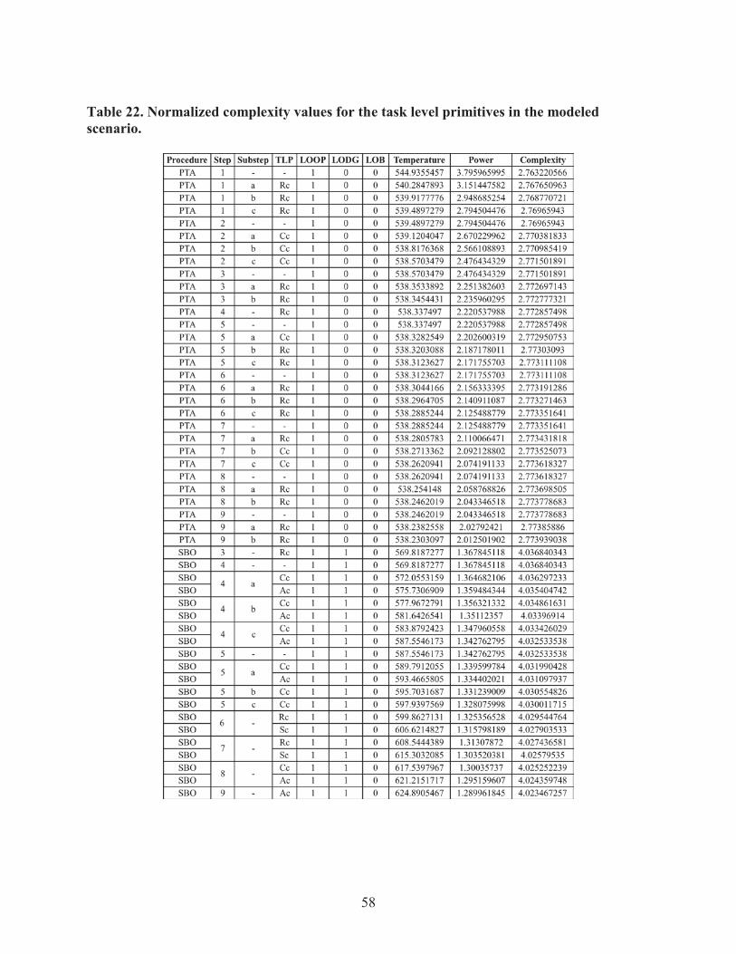
58

Table 22. Normalized complexity values for the task level primitives in the modeled scenario.

Procedure Step Substep TLP LOOP LODG LOB Temperature Power Complexity

PTA 1 - - 1 0 0 544.9355457 3.795965995 2.763220566PTA 1 a Rc 1 0 0 540.2847893 3.151447582 2.767650963

PTA I b Rc 1 0 0 539.9177776 2.948685254 2.768770721

PTA 1 c Rc 1 0 0 539.4897279 2.794504476 2.76965943

PTA 2 - - 1 0 0 539.4897279 2.794504476 2.76965943

PTA 2 a Cc 1 0 0 539.1204047 2.670229962 2.770381833

PTA 2 b Cc 1 0 0 538.8176368 2.566108893 2.770985419

PTA 2 c Cc 1 0 0 538.5703479 2.476434329 2.771501891

PTA 3 - - 1 0 0 538.5703479 2.476434329 2.771501891

PTA 3 a Rc 1 0 0 538.3533892 2.251382603 2.772697143

PTA 3 b Rc 1 0 0 538.3454431 2.235960295 2.772777321

PTA 4 - Rc 1 0 0 538.337497 2.220537988 2.772857498

PTA 5 - - 1 0 0 538.337497 2.220537988 2.772857498

PTA 5 a Cc 1 0 0 538.3282549 2.202600319 2.772950753

PTA 5 b Rc 1 0 0 538.3203088 2.187178011 2.77303093

PTA 5 c Rc 1 0 0 538.3123627 2.171755703 2.773111108PTA 6 - - 1 0 0 538.3123627 2.171755703 2.773111108

PTA 6 a Rc 1 0 0 538.3044166 2.156333395 2.773191286

PTA 6 b Rc 1 0 0 538.2964705 2.140911087 2.773271463

PTA 6 c Rc 1 0 0 538.2885244 2.125488779 2.773351641

PTA 7 - - 1 0 0 538.2885244 2.125488779 2.773351641

PTA 7 a Rc 1 0 0 538.2805783 2.110066471 2.773431818

PTA 7 b Cc 1 0 0 538.2713362 2.092128802 2.773525073

PTA 7 c Cc 1 0 0 538.2620941 2.074191133 2.773618327

PTA 8 - - 1 0 0 538.2620941 2.074191133 2.773618327

PTA 8 a Rc 1 0 0 538.254148 2.058768826 2.773698505

PTA 8 b Rc 1 0 0 538.2462019 2.043346518 2.773778683

PTA 9 - - 1 0 0 538.2462019 2.043346518 2.773778683

PTA 9 a Rc 1 0 0 538.2382558 2.02792421 2.77385886

PTA 9 b Rc 1 0 0 538.2303097 2.012501902 2.773939038

SBO 3 - Rc 1 1 0 569.8187277 1.367845118 4.036840343

SBO 4 - 1 1 0 569.8187277 1.367845118 4.036840343

SBO Cc 1 1 0 572.0553159 1.364682106 4.036297233

SBO Ac 1 1 0 575.7306909 1.359484344 4.035404742

SBO4 b

Cc 1 1 0 577.9672791 1.356321332 4.034861631

SBO Ac 1 1 0 581.6426541 1.35112357 4.03396914

SBO4 c

Cc 1 1 0 583.8792423 1.347960558 4.033426029

SBO Ac 1 1 0 587.5546173 1.342762795 4.032533538

SBO 5 - 1 1 0 587.5546173 1.342762795 4.032533538

SBO5

Cc 1 1 0 589.7912055 1.339599784 4.031990428

SBO Ac 1 1 0 593.4665805 1.334402021 4.031097937

SBO 5 b Cc 1 1 0 595.7031687 1.331239009 4.030554826

SBO 5 c Cc 1 1 0 597.9397569 1.328075998 4.030011715

SBO6 -

Rc 1 1 0 599.8627131 1.325356528 4.029544764

SBO Sc 1 1 0 606.6214827 1.315798189 4.027903533

SBO7

Rc 1 1 0 608.5444389 1.31307872 4.027436581

SBO Sc 1 1 0 615.3032085 1.303520381 4.02579535

SBO8 -

Cc 1 1 0 617.5397967 1.30035737 4.025252239

SBO Ac 1 1 0 621.2151717 1.295159607 4.024359748

SBO 9 - Ac 1 1 0 624.8905467 1.289961845 4.023467257

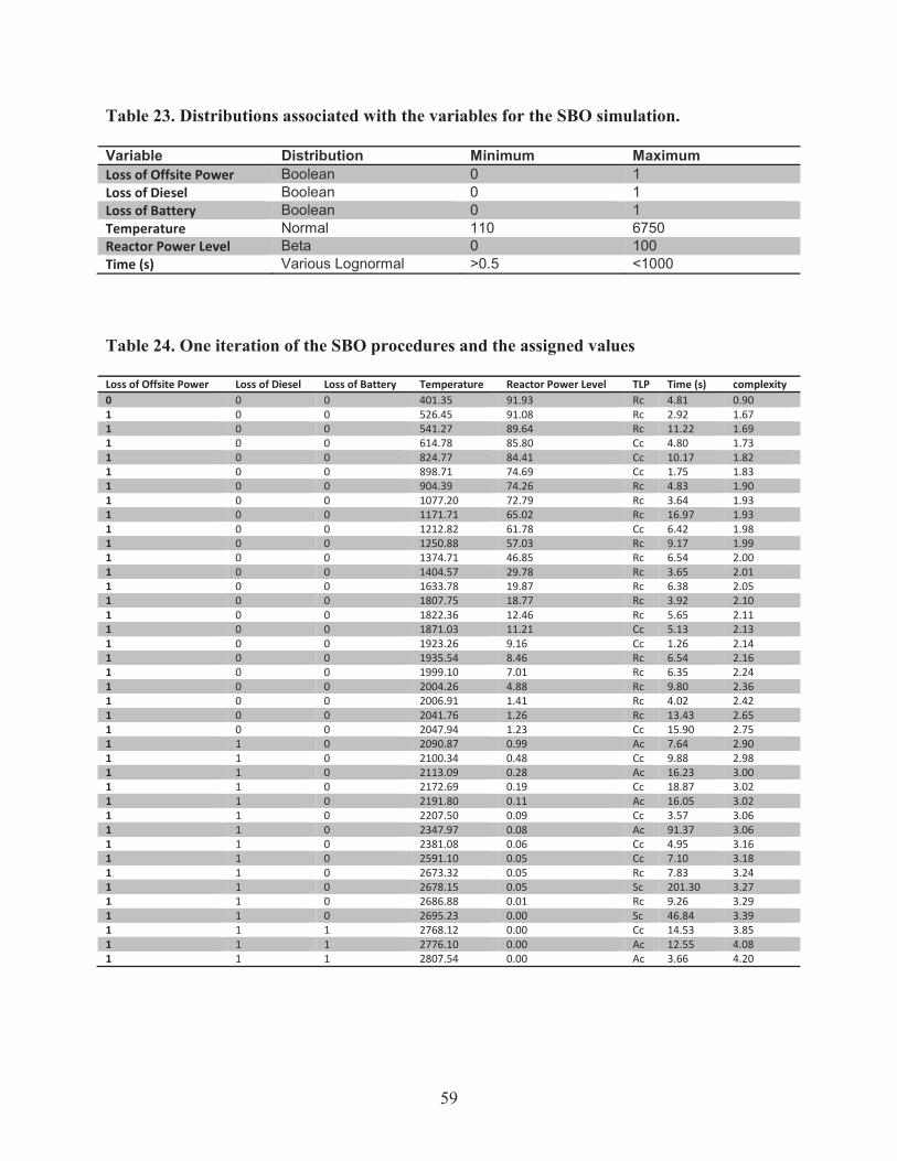
59

Table 23. Distributions associated with the variables for the SBO simulation.

Variable Distribution Minimum MaximumLoss of Offsite Power Boolean 0 1Loss of Diesel Boolean 0 1Loss of Battery Boolean 0 1Temperature Normal 110 6750Reactor Power Level Beta 0 100Time (s) Various Lognormal >0.5 <1000

Table 24. One iteration of the SBO procedures and the assigned values

Loss of Offsite Power Loss of Diesel Loss of Battery Temperature Reactor Power Level TLP Time (s) complexity 0 0 0 401.35 91.93 Rc 4.81 0.90 1 0 0 526.45 91.08 Rc 2.92 1.67 1 0 0 541.27 89.64 Rc 11.22 1.69 1 0 0 614.78 85.80 Cc 4.80 1.73 1 0 0 824.77 84.41 Cc 10.17 1.82 1 0 0 898.71 74.69 Cc 1.75 1.83 1 0 0 904.39 74.26 Rc 4.83 1.90 1 0 0 1077.20 72.79 Rc 3.64 1.93 1 0 0 1171.71 65.02 Rc 16.97 1.93 1 0 0 1212.82 61.78 Cc 6.42 1.98 1 0 0 1250.88 57.03 Rc 9.17 1.99 1 0 0 1374.71 46.85 Rc 6.54 2.00 1 0 0 1404.57 29.78 Rc 3.65 2.01 1 0 0 1633.78 19.87 Rc 6.38 2.05 1 0 0 1807.75 18.77 Rc 3.92 2.10 1 0 0 1822.36 12.46 Rc 5.65 2.11 1 0 0 1871.03 11.21 Cc 5.13 2.13 1 0 0 1923.26 9.16 Cc 1.26 2.14 1 0 0 1935.54 8.46 Rc 6.54 2.16 1 0 0 1999.10 7.01 Rc 6.35 2.24 1 0 0 2004.26 4.88 Rc 9.80 2.36 1 0 0 2006.91 1.41 Rc 4.02 2.42 1 0 0 2041.76 1.26 Rc 13.43 2.65 1 0 0 2047.94 1.23 Cc 15.90 2.75 1 1 0 2090.87 0.99 Ac 7.64 2.90 1 1 0 2100.34 0.48 Cc 9.88 2.98 1 1 0 2113.09 0.28 Ac 16.23 3.00 1 1 0 2172.69 0.19 Cc 18.87 3.02 1 1 0 2191.80 0.11 Ac 16.05 3.02 1 1 0 2207.50 0.09 Cc 3.57 3.06 1 1 0 2347.97 0.08 Ac 91.37 3.06 1 1 0 2381.08 0.06 Cc 4.95 3.16 1 1 0 2591.10 0.05 Cc 7.10 3.18 1 1 0 2673.32 0.05 Rc 7.83 3.24 1 1 0 2678.15 0.05 Sc 201.30 3.27 1 1 0 2686.88 0.01 Rc 9.26 3.29 1 1 0 2695.23 0.00 Sc 46.84 3.39 1 1 1 2768.12 0.00 Cc 14.53 3.85 1 1 1 2776.10 0.00 Ac 12.55 4.08 1 1 1 2807.54 0.00 Ac 3.66 4.20

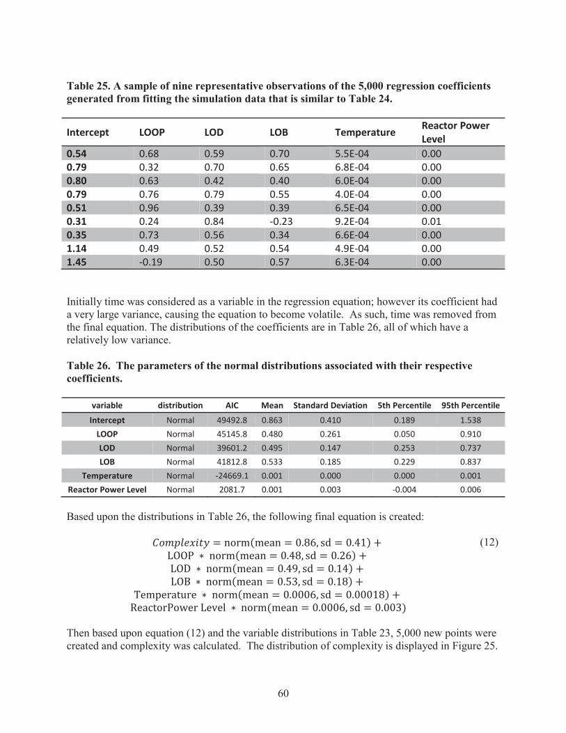
60

Table 25. A sample of nine representative observations of the 5,000 regression coefficients generated from fitting the simulation data that is similar to Table 24.

Intercept LOOP LOD LOB Temperature Reactor Power Level

0.54 0.68 0.59 0.70 5.5E-04 0.00 0.79 0.32 0.70 0.65 6.8E-04 0.00 0.80 0.63 0.42 0.40 6.0E-04 0.00 0.79 0.76 0.79 0.55 4.0E-04 0.00 0.51 0.96 0.39 0.39 6.5E-04 0.00 0.31 0.24 0.84 -0.23 9.2E-04 0.01 0.35 0.73 0.56 0.34 6.6E-04 0.00 1.14 0.49 0.52 0.54 4.9E-04 0.00 1.45 -0.19 0.50 0.57 6.3E-04 0.00

Initially time was considered as a variable in the regression equation; however its coefficient had a very large variance, causing the equation to become volatile. As such, time was removed from the final equation. The distributions of the coefficients are in Table 26, all of which have a relatively low variance.

Table 26. The parameters of the normal distributions associated with their respective coefficients.

variable distribution AIC Mean Standard Deviation 5th Percentile 95th Percentile Intercept Normal 49492.8 0.863 0.410 0.189 1.538

LOOP Normal 45145.8 0.480 0.261 0.050 0.910 LOD Normal 39601.2 0.495 0.147 0.253 0.737 LOB Normal 41812.8 0.533 0.185 0.229 0.837

Temperature Normal -24669.1 0.001 0.000 0.000 0.001 Reactor Power Level Normal 2081.7 0.001 0.003 -0.004 0.006

Based upon the distributions in Table 26, the following final equation is created:

= norm(mean = 0.86, sd = 0.41) + LOOP norm(mean = 0.48, sd = 0.26) + LOD norm(mean = 0.49, sd = 0.14) + LOB norm(mean = 0.53, sd = 0.18) +

Temperature norm(mean = 0.0006, sd = 0.00018) + ReactorPower Level norm(mean = 0.0006, sd = 0.003)

(12)

Then based upon equation (12) and the variable distributions in Table 23, 5,000 new points were created and complexity was calculated. The distribution of complexity is displayed in Figure 25.

61

Figure 25. Distribution of complexity when using equation (12) and the variable distributions from Table 23.

While complexity does appear to have a slight lognormal distribution, it generally fits a normal distribution, with a vast majority of the complexity values above 1. This distribution is attributed to the fact that the complexity space being explored has LOOP, LODG, and LOB about to occur. Therefore, this is an emergency space that is well outside the normal operation of a nuclear power plant, and this does not retain a lognormal distribution like the SPAR-H data from Boringet al. (2006) indicated.

Overall equation (12) preforms well with the variable distributions displayed in Table 23 and is recommended for use when assessing the level of complexity a control room operator experiences during SBO.

7.7.2.3 Comparing the Linear and Stochastic Models of Complexity

As part of the analysis, we have investigated the temporal profile of the complexity factor as a function of time for both the linear and the stochastic model. As an example we have chosen the scenario where 1000 seconds after LOOP conditions, the EDG is lost, and 200 seconds after this last event the battery system is also lost.

00 -.1'

ooCI.

0

CI

0

O

Complexity Distribution

Tin-2 0 2 4 6 8 10

complexity

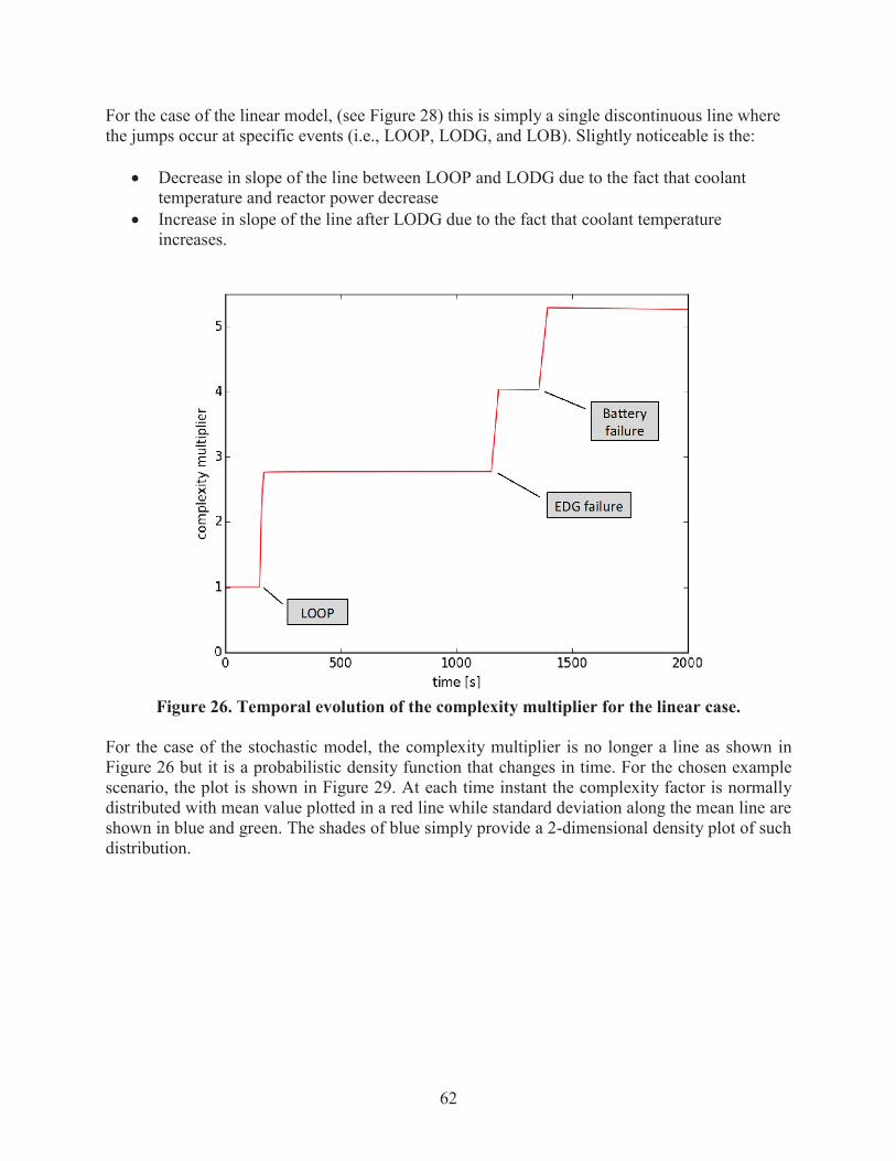
62

For the case of the linear model, (see Figure 28) this is simply a single discontinuous line where the jumps occur at specific events (i.e., LOOP, LODG, and LOB). Slightly noticeable is the:

Decrease in slope of the line between LOOP and LODG due to the fact that coolant temperature and reactor power decreaseIncrease in slope of the line after LODG due to the fact that coolant temperature increases.

Figure 26. Temporal evolution of the complexity multiplier for the linear case.

For the case of the stochastic model, the complexity multiplier is no longer a line as shown in Figure 26 but it is a probabilistic density function that changes in time. For the chosen example scenario, the plot is shown in Figure 29. At each time instant the complexity factor is normally distributed with mean value plotted in a red line while standard deviation along the mean line are shown in blue and green. The shades of blue simply provide a 2-dimensional density plot of such distribution.

LOOP

560

Batteryfailure

EDG failure

1000

time [s]

1500 2000

63

Figure 27. Temporal evolution of the complexity multiplier for the stochastic case.

7.8 Quantifying Operator Performance

Operator performance was quantified as a final HEP value using the GOMS-HRA and SPAR-Hnominal HEP values. Table 27 below shows the nominal HEP values, the PSF multiplier, and the final HEP values for each procedure step modeled in the simulation. SPAR-H and GOMS-HRA were both included to support comparisons and reveal any potential discrepancies between the two methods.

5

4

mean

mean-sigma

— mean+sigma

tiy

LOOP

Batteryfailure

EDG failure

00 500 1000

time [s]

1500 2000

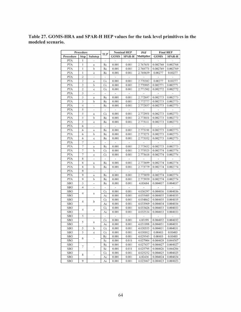
64

Table 27. GOMS-HRA and SPAR-H HEP values for the task level primitives in the modeled scenario.

ProcedureTLP

Nominal HEP PSFMultiplier

Final HEP

Procedure Step Substep GOMS SPAR-H GOMS SPAR-H

PTA 1 - - - - - -

PTA 1 a Rc 0.001 0.001 2.767651 0.002768 0.002768

PTA 1 b Rc 0.001 0.001 2.768771 0.002769 0.002769

PTA 1 c Rc 0.001 0.001 2.769659 0.00277 0.00277

PTA 2 - - - - - - -

PTA 2 a Cc 0.001 0.001 2.770382 0.00277 0.00277 1

PTA 2 b Cc 0.001 0.001 2.770985 0.002771 0.002771

PTA 2 c Cc 0.001 0.001 2.771502 0.002772 0.002772

PTA 3 - - - - - - -

PTA 3 a Rc 0.001 0.001 2.772697 0.002773 0.002773

PTA 3 b Rc 0.001 0.001 2.772777 0.002773 0.002773

PTA 4 - Rc 0.001 0.001 2.772857 0.002773 0.002773

PTA 5 - - - - - - -

PTA 5 a Cc 0.001 0.001 2.772951 0.002773 0.002773

PTA 5 b Rc 0.001 I 0.001 2.773031 0.002773 0.002773

PTA 5 c Rc 0.001 0.001 2.773111 0.002773 0.002773

PTA 6 - - - - - - -PTA 6 a Rc 0.001 0.001 2.773191 0.002773 0.002773

PTA 6 b Rc 0.001 0.001 2.773271 0.002773 0.002773

PTA 6 c Rc 0.001 0.001 2.773352 0.002773 0.002773PTA 7 - - - - - - -

PTA 7 a Rc 0.001 0.001 2.773432 0.002773 0.002773PTA 7 b Cc 0.001 0.001 2.773525 0.002774 0.002774

PTA 7 c Cc 0.001 0.001 2.773618 0.002774 0.002774

PTA 8 - - - - - - -

PTA 8 a Rc 0.001 0.001 2.773699 0.002774 0.002774

PTA 8 b Rc 0.001 0.001 2.773779 0.002774 0.002774

PTA 9 - - - - - - -

PTA 9 a Rc 0.001 0.001 2.773859 0.002774 0.002774

PTA 9 b Rc 0.001 0.001 2.773939 0.002774 0.002774

SBO 3 - Rc 0.001 0.001 4.03684 0.004037 0.004037

SBO 4 - - - - - - -

SBO4 a

Cc 0.001 0.001 4.036297 0.004036 0.004036

SBO Ac 0.001 0.001 4.035405 0.004035 0.004035

SBO4 b

Cc 0.001 0.001 4.034862 0.004035 0.004035

SBO Ac 0.001 0.001 4.033969 0.004034 0.004034

SBO4 c

Cc 0.001 0.001 4.033426 0.004033 0.004033

SBO Ac 0.001 0.001 4.032534 0.004033 0.004033

SBO 5 - - - - - -

SBO5

Cc 0.001 0.001 4.03199 0.004032 0.004032

SBO Ac 0.001 0.001 4.031098 0.004031 0.004031SBO 5 b Cc 0.001 0.001 4.030555 0.004031 0.004031

SBO 5 c Cc 0.001 0.001 4.030012 0.00403 0.00403

SBO6 -

Rc 0.001 0.001 4.029545 0.00403 0.00403

SBO Sc 0.001 0.011 4.027904 0.004028 0.044307 '

SBO-

Rc 0.001 0.001 4.027437 0.004027 0.004027SBO Sc 0.001 0.011 4.025795 0.004026 0.044284

SBOx

Cc 0.001 0.001 4.025252 0.004025 0.004025

SBO Ac 0.001 0.001 4.02436 0.004024 0.004024

SBO 9 - Ac 0.001 0.001 4.023467 0.004023 0.004023

65

7.9 Implementation of HUNTER Modules within RAVEN

The modeling of the HUNTER module has been implemented as a sequential process. Since each procedure (either PTA or SBO) is composed of a set of steps, HUNTER has been similarly coded as shown in Figure 28. In order to complete the procedure, each single step needs to be completed. Recall that each procedure step is characterized by a probability density function (pdf; i.e., the time to complete each step is not fixed in time but it is uncertain) and a nominal HEP value.

Figure 28. HUNTER modeling scheme for each procedure.

In order to complete each step, two conditions need to be satisfied:

1. The time required to complete the step is passed, and,2. The completion has to be successful.

The HUNTER modeling of each procedure step has been implemented as shown in Figure 29:

a) Calculate the time required to complete the step: this is performed by randomly sampling a time value from the step probability density function

b) Wait for the step completion while the RELAP-7 simulation is runningc) Once the time has passed, calculate the value of HEP; here the complexity factor is first

calculated given the information about:a. LOOP statusb. Power levelc. Coolant core outlet temperatured. DG statuse. Battery status

As indicated in Section 7.7.2, two models are considered: a linear and a stochastic complexity model. Once the complexity factor is determined, it multiplies the nominal value of HEP in order to obtain the final HEP value.

Enter

Procedure

Complete Step 1

Complete Step 2

•

.

Complete Step n-1

Complete Step n

r

Exit Procedure

,

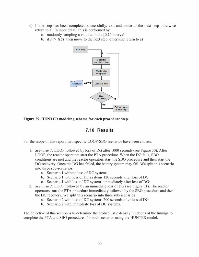
66

d) If the step has been completed successfully, exit and move to the next step otherwise return to a). In more detail, this is performed by:

a. randomly sampling a value in the [0,1) intervalb. if > then move to the next step, otherwise return to a)

Figure 29. HUNTER modeling scheme for each procedure step.

7.10 Results

For the scope of this report, two specific LOOP-SBO scenarios have been chosen:

1. Scenario 1: LOOP followed by loss of DG after 1000 seconds (see Figure 30). After LOOP, the reactor operators start the PTA procedure. When the DG fails, SBO conditions are met and the reactor operators start the SBO procedure and then start the DG recovery. Once the DG has failed, the battery system may fail. We split this scenario into three sub-scenarios:

a. Scenario 1 without loss of DC systemsb. Scenario 1 with loss of DC systems 120 seconds after loss of DGc. Scenario 1 with loss of DC systems immediately after loss of DGs

2. Scenario 2: LOOP followed by an immediate loss of DG (see Figure 31). The reactor operators start the PTA procedure immediately followed by the SBO procedure and then the DG recovery. We split this scenario into three sub-scenarios

a. Scenario 2 with loss of DC systems 200 seconds after loss of DGb. Scenario 2 with immediate loss of DC systems.

The objective of this section is to determine the probabilistic density functions of the timings to complete the PTA and SBO procedures for both scenarios using the HUNTER model.

Enter Step -,

[ —,--- --

Plant Status

_.,--- --

.4.1'4

t

Calculatecompletion time

Wait for stepcompletion

Calculate HEP

o

7- ,Exit and moveto next step

k— r

67

Figure 30. Plot of Scenario 1.

Figure 31. Plot of Scenario 2.

Hot leg coo

lant

tem

pera

ture

[C]

Hot leg co

olan

t te

mper

atur

e [C]

1000

900

800

700

600

500

TSA proc. IF30 proc.

EDG FailureTime

LOOPSBO

EDG recovery

-111Battery failure

0 500 1000 1500 2000 2500 3000 3500 4000

Time [s]

1000

900

800

700

600

E DG recovery

MIWBattery failure

500 0 500 ' ' '1000 1500 2000 2500 3000 3500

Time [s]

4000

68

7.11 Analysis of Scenario 1a

In Scenario 1a, the LODG occurs 1000 seconds after LOOP condition. By Monte-Carlo sampling, we have determined the probabilistic density function of completing the PTA and SBO procedures. These distributions are shown in Figure 32 and Figure 33for the PTA and SBO procedures respectively. Both figures also compare the distributions of the same procedure obtained using both the linear and the stochastic model. All 4 plots shown in Figure 32 and Figure 33also indicate:

The histogram of the values numerical values obtained by using Monte-Carlo sampling (green bars)The plot of the lognormal distribution that fits the obtained data (red line) Three characteristics parameters for a log-normal fitting for the obtained data: shape, loc and scale2

The minimum and maximum values of the obtained data.

Figure 32. Distribution of the timing to perform PTA procedure (Scenario 1a).

2 Given the probabilistic density function ( , ) of a variable being lognormally

distributed with shape parameter is: ( , ) = ( )

. The and parameters are used to shift and scale the distribution so that ( , , , ) is identically equivalent to ( , ) with = .

0.014

0.012

0.010

0.008

linear model ; nominal HEP = 0.001

0.006

0.004

0.002

0.0000 100 200

dup• 0.19kr —36.07srak —106.33

nux —691:19

300 400 500 600

time (51

700

0.014

0.012

0.010

0.008

0.006

0.004

0.002

0.0000

stochastic model ; nominal HEP = 0.001

100 200 300 400

time (s1

500 600 700

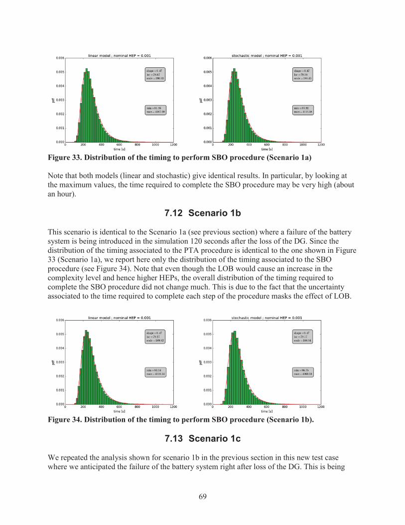
69

Figure 33. Distribution of the timing to perform SBO procedure (Scenario 1a)

Note that both models (linear and stochastic) give identical results. In particular, by looking at the maximum values, the time required to complete the SBO procedure may be very high (about an hour).

7.12 Scenario 1b

This scenario is identical to the Scenario 1a (see previous section) where a failure of the battery system is being introduced in the simulation 120 seconds after the loss of the DG. Since the distribution of the timing associated to the PTA procedure is identical to the one shown in Figure 33 (Scenario 1a), we report here only the distribution of the timing associated to the SBO procedure (see Figure 34). Note that even though the LOB would cause an increase in the complexity level and hence higher HEPs, the overall distribution of the timing required to complete the SBO procedure did not change much. This is due to the fact that the uncertainty associated to the time required to complete each step of the procedure masks the effect of LOB.

Figure 34. Distribution of the timing to perform SBO procedure (Scenario 1b).

7.13 Scenario 1c

We repeated the analysis shown for scenario 1b in the previous section in this new test case where we anticipated the failure of the battery system right after loss of the DG. This is being

0.006

0.005

0.004

0.003

0.002

0.001

0.0000

0.006

0.005

0.004

0.003

0.002

0.001

0

700


400 600

time (sl

800

Amp.. 0 17111. —73 07role — WO 03

I13,,1:oaii,X.

1000 1700

0.006

0.005

0.004

0.003

0.002

0.001

0.0000

linear model ; nominal HEP = 0.0010.006

4mpe : 0.47 0.005kr —79.27stale 1851.62

0.004

0.003

n110,8224max —4018.11

0.002

0.001

0.00000 200 400 600 800 1000 1700

time (s)

stochastic model ; nominal HE!, = 0.001

Ave 0.47kr —7956scale =188.42

.1011,,1—_892101.15.58)

400 600 800 1000 1200

time (s1

stochastic model ; nominal HE!, = 0.001

khope : : 0.47kr —79.17Folk —188.94

olio —85.75max — 1960.18

400 600 800 1000 1200

time fsj

70

done to verify the effect of the loss of battery on the overall distribution of the timing required to complete the SBO procedure. Again (see Figure 35), the impact of the loss of battery can be measured by looking at the slight increase of the characteristic parameters of the fitted log-normal distribution and at the max of the obtained values.

Figure 35. Distribution of the timing to perform SBO procedure (Scenario 1c).

7.14 Scenario 2a

In Scenario 2a, the DG fails right after LOOP while the battery system fails after 200 seconds. In this situation, the operators perform in sequence the PTA and the SBO procedures. In this section, we report the timing associated to complete both procedures. Since the distribution of this time is the time convolution of the distribution to complete the PTA and SBO procedure, we expect to obtain similar lognormal distribution but with higher values of mean and standard deviation. This is confirmed by looking at Figure 36.

Figure 36. Distribution of the timing to perform the sequence of PTA and SBO procedures (Scenario 2a).

7.15 Scenario 2b: LOOP/LODG/LOB

This scenario is similar to Scenario 2a except LOB happens right after LODG. Thus, all electric power is lost. Given the observations reported for scenarios 1b or 1c, we expect a slight

linear model ; nominal HEP = 0.0010.0060.006

0.005 ,hape 0.47lw —7957wale —189.05

0.005

0.004 0.004

0.003 0.003

mat —82.26man .115815

0.002

0.001

0.002

0.001

0.0000 0.0000200 400 600 800 1000 1200

time Is)

0.006

0.005

0.004

0.003

0.002

0.001

0.000


>lawn =0.38loe-239.71wale .259.03

rnin .,- 249.21max 4774.41

500 1000 1500 2000

time Isl

0.006

0.005

0 003

-a 0 003

0 cc )

0.001

0.000o

stochastic model ; nominal MEP = 0.001

400 600

time NI

800

:hope 0.47lw —78.3awale —190.13

min .10.01 )m..-5070.30

1000


11161.--1000

time NJ

1200

Amp, 0.33Ice —239.54wale —257.71

—2421.7574619)

1500 2000

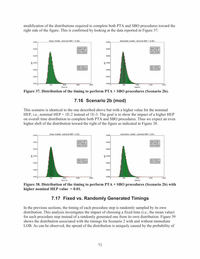
71

modification of the distributions required to complete both PTA and SBO procedures toward the right side of the figure. This is confirmed by looking at the data reported in Figure 37.

Figure 37. Distribution of the timing to perform PTA + SBO procedures (Scenario 2b).

7.16 Scenario 2b (mod)

This scenario is identical to the one described above but with a higher value for the nominal HEP, i.e., nominal HEP = 1E-2 instead of 1E-3. The goal is to show the impact of a higher HEP on overall time distribution to complete both PTA and SBO procedures. Thus we expect an even higher shift of the distribution toward the right of the figure as indicated in Figure 38.

Figure 38. Distribution of the timing to perform PTA + SBO procedures (Scenario 2b) with higher nominal HEP value = 0.01.

7.17 Fixed vs. Randomly Generated Timings

In the previous sections, the timing of each procedure step is randomly sampled by its own distribution. This analysis investigates the impact of choosing a fixed time (i.e., the mean value) for each procedure step instead of a randomly generated one from its own distribution. Figure 39shows the distribution associated with the timings for Scenario 2 with and without immediate LOB. As can be observed, the spread of the distribution is uniquely caused by the probability of

0.006

0.005

0.004

0.003

0.002

0.001

0.0000

0.006

0.005

0.004

0.003

0.002

0.001

0.000o


411\pl. 0.3$

Ice —240.53ecak —258.32

1116,,1:620244.374. 38)

500 1000

time lsl

1500 2000


'hope =0.37k245.10

kak =279.32

min-249.73max — 4149.2:3

500 1000 1500 2000

time ls)

0.006

0.005

0.004

0.003

0.002

0.001

0.0000

0.006

0.005

0 003

.! 0 003

0.002

0.001

stochastic model ; nominal HEP = 0.001

kuipe 0.39Ice —241.18arak —255.96

rnirnr—_21:717..56mo 02)

1000 1500 2000

time Is)


0.0 000

aisape .0.35146,24127Beak =261.68

arlint 2:S10.647mo 65)

1C08 1500 2000

72

failing a single step, which causes the step to be repeated. Hence, in this case, the impact of LOBis more evident.

Figure 39. Distribution of the timing to perform PTA + SBO procedures using the linear complexity model for LOOP+LODG with (left) and without (right) LOB.

0.10

0.08

0.06

0.04

0.02

0.0250

linear model ; nominal NEP = 0.001

max - 600..I.1

111500 550

time (0

600 650

0.10

0.08

0.06

0.04

0.02

0.0250

linear model ; nominal NEP = 0.001

500 550

time (s)

600 650

73


74

8. CONCLUSIONS

8.1 Accomplishments of HUNTER Modeling

HRA is but one part of the larger PRA framework. HRA interacts with the PRA model; however, HRA has often been performed as a standalone analysis. HUNTER provides the possibility to reduce this disconnect by interfacing HRA and PRA into a single RAVEN-HUNTER framework capable of dynamic simulation based modeling. This report demonstrated a successful implementation of the RAVEN-HUNTER framework with dynamic PSFs autopopulated based on high-fidelity thermal-hydraulic models of nuclear power plant behavior during a station blackout scenario. This approach should not be seen as simply replacing traditional HRA with a new modeling form of HRA, but rather as a tool to better integrate human performance (and models) into areas of risk analysis where it has not been included thus far. As the demonstration in this report is a simplified test case, the full capabilities of HUNTER are not realized.HUNTER can model many more features when additional PSFs are incorporated, detailed aspects of the plant parameters are included, and the scenarios become more diverse and contain several paths and possible end states.

This demonstration has also shown how the GOMS-HRA approach can be used to decompose a scenario into standardized units of task level primitives. This allows for quantification at a level where autopopulating PSFs is possible and provides consistency in how a scenario is decomposed and quantified, which is something that has been previously lacking in HRA (Rasmussen & Laumann, 2016) – however this aspect is a critical part of a computationally based approach to HRA. The use of GOMS-HRA task level primitives and autopopulated PSFs allows dynamic modeling and dynamic quantification. This dynamic approach can be used to provide a more comprehensive image of risk changes throughout the unfolding of an event as opposed to the snapshot of a static (or “averaged”) event captured with traditional HRA.

8.2 Limitations of HUNTER Modeling

The work in this document reflects efforts to demonstrate CBHRA in a nuclear power plant station blackout scenario. As this is the initial proof of concept, a number of concessions were necessary to ensure this project achieved reasonable results without unduly spreading our efforts across overly ambitions research aims. A fully comprehensive simulation of the operator and the entire gamut of performance behaviors was beyond the scope of this research, but future efforts are underway to refine the methods and work towards this aim. As a result, a number of limitations must be disclosed.

First, the level of detail in terms of actions within the procedures was restricted to systems of functionally related components as opposed to specific components themselves. For example, in procedures found within an actual plant, a specific procedure step would entail multiple components and their associated indicators and controls, such as the series of main steam isolation valves. In our simulation, verifying the main steam isolation valves closed after the initial plant trip event was considered a single action taken by the operator, but in reality this consists of visually verifying each valve sequentially. This specific example likely did not

75

generate any meaningful discrepancies between actual operator behavior and the simulation, but since this approach was followed to reduce the complexity of the simulation, it is possible that nuanced errors, such as visually overlooking a single valve position, were not accurately represented in the simulation. Further refinement and added complexity to the procedures modeled in the simulation can enhance the accuracy of the simulation and yield more generalizable results during future efforts within this same line of research.

The other primary limitation concerns the PSFs used for quantification of human error in the model. This work only considered complexity as inputs to calculate the overall HEP within each timestep. There are more PSFs that also impact the likelihood of operator error. The HUNTER modelling approach is capable of including these PSFs with little modification required. Future efforts are aimed providing the functionality to support more PSFs and the complicated interrelations they form between themselves and ultimately on human error.

8.3 Future Research on Quantification

8.3.1 Background

The quantification approach currently employed in HUNTER is simplified, dynamically calculating a PSF and treating it as a multiplier on the nominal HEP. This approach becomes strained for more complex modeling, including cases where the effects of multiple concurrent PSFs must be calculated. Future research will look at alternate ways of quantifying HEPs as well as accounting for the interrelationships between PSFs. An approach involving Bayesian network modeling holds promise for providing a scalable quantification model for HUNTER.

8.3.2 Bayesian Network Basic Concepts

Bayesian Networks (BNs) provide a framework for developing a detailed mathematical model encoding the causal relationships between PSFs and errors. BNs address many known issues with current HRA methods. First, we explain the basic structure of a BN. Mathematically, a BN is a quantitative causal model that expresses the joint probability distribution of a universe of events in terms of a set of nodes, a graph, and a set of conditional probability distributions.

BNs can provide a detailed, causal picture of the interactions between human and machine. This enables meeting a key challenge for CBHRA: to move beyond a focus on human error into a focus on the interactions between human and machine. (Groth and Swiler, 2013). Groth andSwiler (2013) also lay out a number of important features of BNs for HRA.

The method builds a probabilistic model that shows relationships between different variables or concepts. In a BN, the variables are called nodes and are graphically represented as a circle/ellipse. The relationships between nodes are displayed as arcs between nodes; these encode mathematical dependence statements. A basic example of a BN that uses PSFs as nodes and displays relationships is shown in Figure 40.

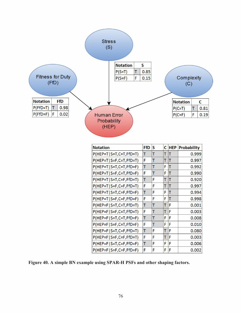
76

Figure 40. A simple BN example using SPAR-H PSFs and other shaping factors.

Fitness for Duty(FfD)

Notation FfD

P(FfD=T) T 0.98

P(FfD=F) F 0.02

Stress(S)

Notation S

P(S=T) T 0.85

P(S=F) F 0.15

Y

Human ErrorProbability(HEP)

Complexity(C)

Notation C

P(C=T) T 0.81

P(C=F) F 0.19

Notation FfD S C HEP Probability

P(H EP=T l S=T,C=T,FfD=T) T T T T 0.999

P(H EP=T l S=F,C=T,FfD=T) F T T T 0.997

P(HEP=T1S=T,C=T,FfD=F) T T F T 0.992

P(HEP=T1S=F,C=T,FfD=F) F T F T 0.990

P(H EP=T l S=T,C=F,FfD=T) T F T T 0.920

P(HEP=T1S=F,C=F,FfD=T) F F T T 0.997

P(HEP=T1S=T,C=F,FfD=F) T F F T 0.994

P(HEP=T1S=F,C=F,FfD=F) F F F T 0.998

P(HEP=F l S=T,C=T,FfD=T) T T T F 0.001

P(HEP=F1S=F,C=T,FfD=T) F T T F 0.003

P(HEP=F1S=T,C=T,FfD=F) T T F F 0.008

P(HEP=F1S=F,C=T,FfD=F) F T F F 0.010

P(HEP=F1S=T,C=F,FfD=T) T F T F 0.080

P(HEP=F1S=F,C=F,FfD=T) F F T F 0.003

P(HEP=F1S=T,C=F,FfD=F) T F F F 0.006

P(HEP=F1S=F,C=F,FfD=F) F F F F 0.002

77

In Figure 40 the three PSFs of fitness for duty (FfD), complexity (C), and stress (S) and the resultant human error probability (HEP)3 are all nodes. Each node in Figure 40 has two possible states: a positive (T) or negative (F) effect on the HEP. The probability of each PSF having a positive vs. negative effect is shown in the tables beside each PSF node. The HEP node is assigned a conditional probability table, which includes the probability of HEP (true or false) given each possible combination of PSFs. Note that the sum of the probabilities of the states for each node must be 1.0.

The influence of PSFs (in blue) is directed to the HEP (in red). Specifically FfD, S, and C are all parent nodes of HFE, and the probability of the HFE depends on the relationship between the PSFs and the HFE as well as the marginal probabilities of the PSFs. The BN propagates information about node states (both observed and unobserved) through the network to obtain probabilities; the underlying mathematics of the BN is explained further in Groth and Swiler (2013).

8.3.3 Dynamic Belief Networks

A DBN is a BN that represents a temporal probability model. Additionally, every hidden Markov model (HMM) can also be translated into a DBN, and all discrete DBNs can be HMMs (Russell and Norvig, 2003). So while the same basic technique can once again be called by different names, there does exist a difference, namely that HMMs tend to be more computationally expensive, with a wider variety in end states.

DBNs are a useful tool for human error modeling. To create a DBN, three pieces of information are needed:

The prior distribution over the nodes, ( )The transition model, ( | )The sensor model, ( | )

The transition model, or transition matrix in the discrete case, changes the BN into a DBN, which allows the nodes to step across time. The sensor model describes the probability of each perception, given the current state. Usually sensor models have an incorporation of Gaussian, or normal, errors added. Error is added to the sensor model because, for example, occasionally an individual may be fit for duty, have low stress and complexity but still incorrectly complete a task. This inclusion of error in the sensor model allows the possibility of capturing human behavior in the model. Additionally, both the transition model and the sensor model are assumed to be stationary, i.e., they do not change when the time steps change, throughout the entire simulation.

3 The red node might also be called the human failure event (HFE), which produces the HEP. Here, for the purposes of simplification, we simply call the node HEP.

78

8.3.4 Advantages of BNs to Enable CBHRA

Several international research groups are working on BNs for HRA, but there has been little work on how these models could be used in a simulation-based framework. Groth and Swiler (2013) outline a number of BN features which are valuable for HRA. Several of these features are worth highlighting for CBHRA.

BNs allow explicit representation of causal structure. Groth and Swiler (2013) and Ekanem and Mosleh (2016) demonstrate how the BN can be expanded to additional levels of detail to inforporate more detailed variables and enable inclusion of information used to assign PSF states. Zwirglmaier et al. (in press) demonstrates how this causal structure can be used to draw a direct map from “PSF details” (that is, observable plant parameters and more detailed decomposition of PSFs such as those discussed in Groth and Mosleh (2012a) and Rasmussen 2015) to PSFs to HEPs. Zwirglmaier also illustrates how the full causal structure can be reduced into a smaller BN using node reduction algorithms.

BNs also allow the modeler to sub-divide the universe into smaller pieces, which can be more easily quantified. This has multiple advantages, including that the BN framework is also compatible with Bayesian updating, which enables using sparse data to update specific aspects of the model (Groth, Smith, and Swiler 2014). Furthermore, BNs conditional independence relationships to eliminate dependencies on unnecessary variables, which produces a substantially simpler expression of the joint probability distribution. It follows that we can also use BNs to create individual BNs for independent tasks or events.

The BN framework can be used to capture PSF-to-PSF interdependency, as illustrated in Groth and Mosleh (2012b). This ability enables capturing a crucial factor missing from current HRA models: cause and effect relationships between PSFs. This is important for traditional HRA to enable capturing PSF relationships within the same event, but also takes on extra importance for CBHRA, where it is necessary to capture PSF relationships across events timesteps. The mechanism for doing this is a repeating temporal model: a Dynamic Bayesian Network (DBN).

8.3.5 BNs for GOMS-HRA Primitives in HUNTER

It has been previously shown that different PSFs have differing effects on the overall behavior of errors (Whaley et al., 2016). As such, the goal is to empirically create sub-models that show which PSFs and PSF details4 are related to specific types of errors. BNs can be used to develop a unique model for each GOMS-HRA primitive. For example, the ability of a reactor operator to follow a procedure that specifies verify is strongly tied to their previous training, overall crew behavior, and control panel design, rather than complexity. The perception is that task complexity, whether high or low, should have little bearing on an operator’s ability to read a

4 A PSF detail is supporting information that defines the PSF. The complexity model presented in Chapter 4 outlines several of the factors that form the overall complexity coefficient. Such factors are PSF details.

79

display. This idea has been explored by Zwirglmaier et al (2015 and in press) through a specific set of PSFs and PSF details, which are causally related to data perception errors.

Figure 41. Verify mini-BN for use within HUNTER (adapted from Zwirglmaier et al., in press).

As such, a similar mini-BN is proposed for the verify primitive as in Figure 41. The structure is proposed but needs to be validated, as nodes can be added or removed based on the typical data available when assessing a power plant operator’s ability to verify data in the procedural steps. In addition to each time step having a different relationship between nodes, transition models and sensor models need to be described thoroughly. Building a collection of mini-BN for the procedure primitives would provide two key additions to the HUNTER framework:

1. Easy reuse of the mini-BNs for creation of a wide range of scenarios. Just as the procedure primitives can be chained together to represent a full range of scenarios, the mini-BNs can likewise be applied to quantify this same range of scenarios.

2. Scalability of the mini-BN to allow incorporation of additional PSFs and PSF details without affecting models that have been built around procedure primitives. In other words, it is possible to increase the model fidelity by refining the mini-BN without rebuilding the entire model of human actions in HUNTER.

Ability to read data

Clear display ofrange for

comparison

Unambiguity

HSI / Enviromental

Environmentnominal

Indications - easy toread and locate

Still determiningplant status

Workload

( Perception of data '4-

More tasks thannormal

Several alarms

Crew trained tounderstand scenario

Priority compared tocurrent task

80

8.4 Future Research on Empirical Data Collection

8.4.1 HRA Empirical Databases

Empirical evidence is a crucial aspect to form the basis for HRA model creation and validation,since without empirical data the model remains merely SME speculation. The lack of adequate human performance data poses the greatest barrier for generating accurate HEP calculations.Ideally, dynamic HRA assessments would be based on comprehensive simulator or plant operations data in order to accurately reflect the contextual factors and human actions during HFEs. Currently, the necessary databases with sufficient detail to support dynamic HRA are not yet available, though recent efforts toward creating a framework to populate these databases appear quite promising. Currently several researchers INL have contributed to the Scenario Authoring, Characterization, and Debriefing Application (SACADA) database (Chang et al., 2014), which has recently become available for potential use in dynamic HRA. International efforts supporting suitable databases for HRA model creation and validation are also underway. The Korea Atomic Energy Research Institute (KAERI) database is projected to be accessiblebetween 2017 and 2018.

8.4.2 SACADA

The SACADA database superseded the Human Event Repository and Analysis (HERA) databaseused in previous HRA efforts (Hallbert et al., 2006). SACADA was developed with many parallel goals, one of which is to support current and future HEP calculations. The variables recorded are aimed at providing sufficient contextual information to support quantification in HRA. The database consists of categorical variables describing the state of the nuclear power plant control room.

8.4.3 KAERI

KAERI is currently developing its own HRA database. The database has not been released in English but is set for a release in the future (Park et al., 2013). Data collection is based on guidelines and multiple assessments. The main goal is to provide for the provision of sufficient and reliable HRA data with the aim to inform second generation HRA methods. KAERI’s efforts should prove informative to HUNTER aims.

8.4.4 HRA Data Studies at Norwegian University of Science and Technology

The Center for Safety and Human Factors is a research group at the Department of Psychology at the Norwegian University of Science and Technology that has experience with HRA through the Petro-HRA project. The Petro-HRA project developed an HRA method tailored specifically for the oil and gas industry. Through this work, several knowledge gaps were identified in the relationship between PSFs and human performance. A human performance focused laboratory is currently being developed with the goal of gaining a better understanding of how factors such as time pressure, training, teamwork, HMI, and alarms influence the performance in major accident scenarios. The laboratory will conduct simulator based studies. At this stage not all of the details

81

are ready (such as the fidelity of the simulator), but it is likely that inputs from this laboratorycan be used in validation or calibration of HUNTER modeling.

8.5 Future Research Demonstrations of HUNTER

In this initial demonstration of HUNTER, the model of the operator consisted of a single PSF and spanned only a single scenario, i.e,. the station blackout event. Future research in HUNTER aims to move toward improving the HUNTER framework to the level in which a plant PRA model can be dynamically simulated. Dynamically modeling a plant PRA entails a large scale effort comprised of simulating accident sequence progressions, plant systems and components, and operator actions. To support this functionality, future work on HUNTER will incorporate more scenarios and the necessary procedures to support the operator models. Additionally, the operator cognitive model will be enhanced by incorporating additional PSFs to capture a more accurate portrayal of the operator and human error likelihoods during scenario evolutions.

82

9. REFERENCES

Abdel-Khalik, H. S., Bang, Y., Kennedy, C., & Hite, J. (2012). Reduced order modeling for nonlinear multi-component models. International Journal for Uncertainty Quantification,2(4).

Acosta, C., & Siu, N. (1993). Dynamic event trees in accident sequence analysis: Application to steam generator tube rupture. Reliability Engineering and System Safety, 41, 135-154.

Alfonsi, A., Rabiti, C., Mandelli, D., Cogliati J., Kinoshita R., & Naviglio, A. (2014). RAVEN and dynamic probabilistic risk assessment: Software overview, in Proceedings of European Safety and Reliability Conference (ESREL 2014), Wroklaw, Poland.

Amendola, A., & Reina, G. (1984). DYLAM-1: A software package for event sequence and consequence spectrum methodology, EUR-9224. Commission of the European Communities.

Anders, D., Berry, R., Gaston, D., Martineau, R., Peterson, J., Zhang, H., & … Zou, L. (2012). Relap-7 level 2 milestone report: Demonstration of a steady state single phase PWR simulation with relap-7, INL/EXT-12-25924. Idaho Falls: Idaho National Laboratory.

Beal, D. J. (2007). Information criteria methods in SAS for multiple linear regression models. 15th Annual South East SAS Users Group (SESUG) Proceedings, South Carolina, Paper SA05.

Bell, B.J., & Holroyd, J. (2009). Review of Human Reliability Assessment Methods, RR679. Buxton, UK: Health and Safety Executive.

Bell, B.J., & Swain, A.D. (1983). A Procedure for Conducting Human Reliability Analysis for Nuclear Power Plants, Final Report, NUREG/CR-2254. Washington, DC: U.S. Nuclear Regulatory Commission.

Boring, R. L. (2012). Fifty years of THERP and human reliability analysis. In Proceedings of the Probabilistic Safety Assessment and Management and European Safety and Reliability Conference (PSAM 11 & ESREL 2012).

Boring, R.L., Whaley, A.M., Tran, T.Q., McCabe, P.H., Blackwood, L.G., & Buell, R.F. (2006). Guidance on Performance Shaping Factor Assignments in SPAR-H, INL/EXT-06-11959.Idaho Falls: Idaho National Laboratory.

Boring, R. L. (2007). Dynamic human reliability analysis: Benefits and challenges of simulating human performance. Risk, Reliability and Societal Safety, 2, 1043-1049.

83

Boring, R. L. (2009). Human reliability analysis in cognitive engineering and system design. In Frontiers of Engineering: Reports on Leading-Edge Engineering from the 2008 Symposium, 103-110.

Boring, R.L. (2010). How Many Performance Shaping Factors are Necessary for Human Reliability Analysis? Proceedings of the Probabilistic Safety Assessment and Management (PSAM10), June 2010. Seattle, WA.

Boring, R.L. (2015). Defining human failure events for petroleum applications of human reliability analysis. Procedia Manufacturing, 3, 1335-1342.

Boring, R.L. et al., (2010). Lessons Learned on Benchmarking from the International Human Reliability Analysis Empirical Study. In Proceedings of the Probabilistic Safety Assessment and Management (PSAM10), Seattle, WA.

Boring, R., Lew, R., Ulrich, T., & Joe, J. (2014). Light Water Reactor Sustainability Program Operator Performance Metrics for Control Room Modernization: A Practical Guide for Early Design Evaluation, INL/EXT-14-31511. Idaho Falls: Idaho National Laboratory.

Boring, R.L., Joe, J.C., & Mandelli, D. (2015). Human performance modeling for dynamic human reliability analysis. Lecture Notes in Computer Science, 9184, 223–234.

Boring, R., Mandelli, D., Joe, J., Smith, C., & Groth, K. (2015). A Research Roadmap for Computation-Based Human Reliability Analysis, INL/EXT-15-36051. Idaho Falls: Idaho National Laboratory.

Boring, R. L., Shirley, R. E., Joe, J. C., & Mandelli, D. (2014). Simulation and Non-Simulation Based Human Reliability Analysis Approaches, INL/EXT-14-33903. Idaho Falls: Idaho National Laboratory.

Bye, A. et al., (2011). International HRA Empirical Study–Phase 2 Report: Results from Comparing HRA Method Predictions to Simulator Data from SGTR Scenarios, NU-REG/IA-0216, Vol. 2. Washington, DC: U.S. Nuclear Regulatory Commission.

Card, S.K., Moran, T.P., & Newell, A. (1980). The key stroke level model for user performance time with interactive systems. Communications of the ACM, 23, 396-410.

Card, S., Moran, T., & Newell, A. (1983). The Psychology of Human-Computer Interaction. Hillsdale, NJ: Lawrence Erlbaum Associates.

Chang, J. Y. et al., (2014). The SACADA database for human reliability and human performance. Reliability Engineering & System Safety, 125, 117–133.

Chandler, F.T., Chang, Y.H.J., Mosleh, A., Marble, J.L., Boring, R.L., & Gertman, D.I. (2006).Human Reliability Analysis Methods: Selection Guidance for NASA. Washington, DC: NASA Office of Safety and Mission Assurance Technical Report.

84

Coyne, K. & Siu N. (2013). Simulation-based analysis for nuclear power plant risk assessment: Opportunities and challenges Proceedings of the ANS Embedded Conference on Risk Management for Complex Socio-Technical Systems, Washington D.C.

Eide, S. A., Gentillon, C. D., Wierman, T. E., & Rasmuson, D. M. (2005). Reevaluation of station blackout risk at nuclear power plants, NUREG/CR-6890 Vol 1. 1986-2004.Washington, DC: U.S. Nuclear Regulatory Commission.

Ekanem, N.J., Mosleh, A., & Shen, S.-H. (2016). Phoenix—A model-based human reliability analysis methodology: Qualitative analysis procedure. Reliability Engineering & System Safety, 145, 301-315.

Electric Power Research Institute (EPRI). (1992). SHARP1—A Revised Systematic Human Action Reliability Procedure, EPRI-101711. Palo Alto: Electric Power Research Institute.

Fodor, J.A. (1983). Modularity of Mind: An Essay on Faculty Psychology. Cambridge, Mass.: MIT Press.

Forester, J., Dang, V.N., Bye, A., Lois, E., Massaiu, S., Broberg, H., Braarud, P.Ø., Boring, R., Männistö, I., Liao, H., Julius, J., Parry, G., & Nelson, P. (2014). The International HRA Empirical Study. Lessons Learned from Comparing HRA Methods Predictions to HAMMLAB Simulator Data, NUREG-2127. Washington, DC: U.S. Nuclear Regulatory Commission.

Forester, J., Kolaczkowski, A., Lois, E., & Kelly, D. (2006). Evaluation of human reliability analysis methods against good practices, NUREG-1842. Washington, DC: US Nuclear Regulatory Commission.

Gardiner, C. W. (1985). Handbook of stochastic methods (Vol. 3). Berlin: Springer.

Gertman, D., Blackman, H., Marble, J., Byers, J., & Smith, C. (2005). The SPAR-H Human Reliability Analysis Method, NUREG/CR-6883. Washington, DC: U.S. Nuclear Regulatory Commission.

Gray, W.D., John, B.E., & Atwood, M.E. (1993). Project Ernestine: A validation of GOMS for prediction and explanation of real-world task performance. Human-Computer Interaction, 8, 237-309.

Groth, K.M., & Mosleh, A. (2012a). A data-informed PIF hierarch for model-based human reliability analysis. Reliability Engineering and System Safety, 108, 154-174.

Groth, K.M., & Mosleh, A. (2012b). Deriving causal Bayesian networks from human reliability analysis data: A methodology and example model. Proceedings of the Institution of Mechanical Engineers, Part O: Journal of Risk and Reliability, 226, 361-379

85

Groth, K. M., Smith, C. L., & Swiler, L. P. (2014). A Bayesian method for using simulator data to enhance human error probabilities assigned by existing HRA methods. Reliability Engineering & System Safety, 128, 32-40.

Groth, K., & Swiler, L. (2013). Bridging the gap between HRA research and HRA practice: A Bayesian network version of SPAR-H. Reliability Engineering and System Safety, 115, 33-42.

Hallbert, B., Boring, R., Gertman, D., Dudenhoeffer, D., Whaley, A., Marble, J., … & Lois, E. (2006). Human event repository and analysis (HERA) system overview, NUREG/CR-6903. Idaho National Laboratory for the US Nuclear Regulatory Commission, Washington, DC.

Helton, J. C., & Davis, F. J. (2003). Latin hypercube sampling and the propagation of uncertainty in analyses of complex systems. Reliability Engineering & System Safety, 81(1), 23-69.

Inaba, K. (2004). Boost C++ Library Programming, Shuwa System, ISBN: 4-7980-0786-2.

International Atomic Energy Agency (IAEA). (1980). Protection System and Related Features in Nuclear Power Plants, Safety Series No. 50-SG-D3. Vienna: International Atomic Energy Agency.

IEEE. (1997). Guide for Incorporating Human Action Reliability Analysis for Nuclear Power Generating Stations, IEEE-1082. New York: Institute of Electrical and Electronics Engineers.

Jang, T. I., Lee, Y. H., Park, J. C., Jeong, Y. S., & Chu, G. I. (2010). Standardization of the Action Verbs used in Emergency Operating Procedures of NPPs.

Kieras, D. (2004). GOMS models for task analysis. In D. Diaper & N. Stanton (Eds.), The Handbook of Task Analysis for Human-Computer Interaction, 83-116. Mahwah, NJ: Lawrence Erlbaum Associations.

Kieras, D. (2006). A Guide to GOMS Model Usability Evaluation Using GOMSL and GLEAN4. University of Michigan technical report.

Kirwan, B., Basra, G. & Taylor-Adams, S.E., (1997). CORE-DATA: A computerized human error database for human reliability support. In Proceedings of the 1997 IEEE Sixth Conference on Human Factors and Power Plants, 1997. “Global Perspectives of Human Factors in Power Generation.” Orlando, FL.

Park, J., Jung, W., Kim, S., Choi, S., Kim, Y., Lee, S., & Dang, V. N. (2013). A guideline to collect HRA data in the simulator of nuclear power plants, KAERI/TR-5206/2013. Korea Atomic Energy Research Institute.

86

Laumann, K. et al., (2014). Analysis of human actions as barriers in major accidents in the petroleum industry, applicability of human reliability analysis methods (Petro-HRA). In Proceedings of the Probabilistic Safety Assessment and Management (PSAM12).Honolulu, HI.

Mandelli, D., Prescott, S., Smith, C., Alfonsi, A., Rabiti, C., Cogliati, J., & Kinoshita, R. (2015). Modeling of a Flooding Induced Station Blackout for a Pressurized Water Reactor Using the RISMC Toolkit. In ANS PSA 2015 International Topical Meeting on Probabilistic Safety Assessment and Analysis Columbia, SC. American Nuclear Society, LaGrange Park, IL.

Mandelli, D., Smith, C., Alfonsi, A., & Rabiti, C. (2014). Overview of new tools to perform safety analysis: BWR station black out test case. In Proceedings of PSAM, 12.

Mandelli, D., Smith, C., Rabiti, C., Alfonsi, A., Youngblood, R., Pascucci, V., ... & Yilmaz, A. (2013). Dynamic PRA: an overview of new algorithms to generate, analyze and visualize data. Proceeding of American Nuclear Society.

Marseguerra, M., Zio, E., Devooght, J., & Labeau, P. E. (1998). A concept paper on dynamic reliability via Monte Carlo simulation. Mathematics and Computers in Simulation, 47(2), 371-382.

Mosleh, A. (2014). PRA: A perspective on strengths, current limitations, and possible improvements. Nuclear Engineering and Technology, 46, 1-10.

Nielsen, J. (1989). Usability engineering at a discount. In G. Salvendy and M.J. Smith, M.J. (Eds.), Designing and Using Human-Computer Interfaces and Knowledge Based Systems, 394-401. Amsterdam: Elsevier Science Publishers.

Park, J., Jung, W., Kim, S., Choi, S., Kim, Y., Lee, S., & Dang, V. N. (2013). A guideline to collect HRA data in the simulator of nuclear power plants. KAERI/TR-5206/2013.

Parry, G.W., Lydell, B.O.Y., Spurgin, A.J., Moienl, P., & Beare, A. (1992). An Approach to the Analysis of Operator Actions in Probabilistic Risk Assessment, TR-100259. Palo Alto: Electric Power Research Institute.

Prescott, S., Smith, C., & Sampath, R. (2015). Incorporating Dynamic 3D Simulation into PRA. In ANS PSA 2015 International Topical Meeting on Probabilistic Safety Assessment and Analysis Columbia, SC, American Nuclear Society, LaGrange Park, IL.

Procedure Professionals Association. (2016). Procedure Writers’ Manual, (PPA AP-907-005,Rev. 2).

Rabiti, C., Alfonsi A., Mandelli, D., Cogliati, J., Martinueau, R., & Smith, C. (2013). Deployment and Overview of RAVEN Capabilities for a Probabilistic Risk Assessment

87

Demo for a PWR Station Blackout, INL/EXT-14-33903. Idaho Falls: Idaho National Laboratory.

Rabiti, C., Mandelli, D., Alfonsi, A., Cogliati, J., & Kinoshita, B. (2013, May). Mathematical framework for the analysis of dynamic stochastic systems with the raven code. In Proceedings of International Conference of mathematics and Computational Methods Applied to Nuclear Science and Engineering (M&C 2013), Sun Valley, ID.

Rasmussen, M. & Laumann, K., (2016). The impact of decomposition level in human reliability analysis quantification. In Proceedings of ESREL2016. Glasgow, Scotland.

Rasmussen, M., Standal, M.I. & Laumann, K., (2015). Task complexity as a performance shaping factor: A review and recommendations in Standardized Plant Analysis Risk-Human Reliability Analysis (SPAR-H) adaption. Safety Science, 76, 228–238.

Rogers, Y., Sharp, H., & Preece, J. (2002). Interaction Design. New York: John Wiley & Sons.

Russell, S., & Norvig, P. (2003). Artificial Intelligence: A Modern Approach, Second Edition. Upper Saddle River: Prentice Hall.

Management Science, 31(6), 719-728.

Spurgin, A. J. (2010). Human Reliability Assessment Theory and Practice. CRC press.

Stanton, N.A., Salmon, P.M., Rafferty, L.A., Walker, G.H., and Baber, C. (2013). Human Factors Methods: A Practical Guide for Engineering and Design, Second Edition. Aldershot, UK: Ashgate Publishing Co.

Swain, A.D., & Guttman, H.E. (1983). Handbook of Human Reliability Analysis with Emphasis on Nuclear Power Plant Applications, NUREG/CR-1278. Washington, DC: U.S. Nuclear Regulatory Commission.

Swain, A. D. (1990). Human reliability analysis: Need, status, trends and limitations. Reliability Engineering & System Safety, 29(3), 301-313.

Todorova, N., Ivanov, K., & Taylor, B. (2003). Pressurized Water Reactor Main Steam Line Break (MSLB) Benchmark. Volume IV: Results of Phase III on Coupled Core-Plant Transient Modeling, 21, 2003.

U.S. Nuclear Regulatory Commission. (1975). WASH 1400 - Reactor Safety Study - An Assessment of Accident Risks in U.S. Commercial Nuclear Power Plants. Washington, DC: U.S. Nuclear Regulatory Commission.

88

U.S. Nuclear Regulatory Commission. (2005). Re-evaluation of station blackout risk at nuclear power plants: Analysis of events, NUREG/CR-6890. Washington, DC: U.S. Nuclear Regulatory Commission.

Whaley, A.M., Xing, J., Boring, R.L., Hendrickson, S.M.L., Joe, J.C., Le Blanc, K.L. and Morrow, S.L. (2016). Cognitive Basis for Human Reliability Analysis. U.S. Nuclear Regulatory Commission, NUREG-2114. Washington, DC: U.S. Nuclear Regulatory Commission.

Williams, J. C. (1988). A data-based method for assessing and reducing human error to improve operational performance. In Conference Record for 1988 IEEE Fourth Conference on Human Factors and Power Plants, 436-450. IEEE.

Williams, J.C. (1992). A User Manual for the HEART Human Reliability Assessment Method. Stockport, UK: DNV Technica.

Wood, S.D. (2000). Extending GOMS to Human Error and Applying It to Error-Tolerant Design. University of Michigan Dissertation in Computer Science and Engineering.

Zwirglmaier, K., Straub, D., & Groth, K. (In press). Capturing cognitive causal paths in human reliability analysis with Bayesian network models. Reliability Engineering and System Safety.

Zwirglmaier, K., Straub, D., & Groth, K. (2015). Framework for a Bayesian network version of IDHEAS. In L. Podofillini (Eds.), Safety and Reliability of Complex Engineered Systems (pp. 3165-3172). London: Taylor & Francis Group.

89

APPENDIX A: LIST OF HUNTER PUBLICATIONS

Boring, R.L. (2015). A dynamic approach to modeling dependence between human failure events. In L. Podofillini (Ed.), Safety and Reliability of Complex Engineered Systems (pp. 2845-2851). London: Taylor & Francis Group.

Boring, R.L., & Herberger, S.M. (2016, in press). Testing subtask quantification assumptions for dynamic human reliability analysis in the SPAR-H method. Proceedings of the 60th International Annual Meeting of the Human Factors and Ergonomics Society.

Boring, R.L., Joe, J.C., & Mandelli, D. (2015). Human performance modeling for dynamic human reliability analysis. Lecture Notes in Computer Science, 9184, 223–234.

Boring, R., Mandelli, D., Joe, J., Smith, C., & Groth, K. (2015). A Research Roadmap for Computation-Based Human Reliability Analysis, INL/EXT-15-36051. Idaho Falls: Idaho National Laboratory.

Boring, R., Mandelli, D., Rasmussen, M., Herberger, S., Ulrich, T., Groth, K., & Smith, C. (2016). Integration of Human Reliability Analysis Models in the Simulation-Based Framework for the Risk-Informed Safety Margin Characterization Toolkit, INL/EXT-16-39015. Idaho Falls: Idaho National Laboratory.

Boring, R., Mandelli, D., Rasmussen, M., Herberger, S., Ulrich, T., Groth, K., & Smith, C. (2016, in press). Human Unimodel for Nuclear Technology to Enhance Reliability (HUNTER): A framework for computation-based human reliability analysis. Proceedings of the Probabilistic Safety Assessment and Management Conference.

Boring, R.L., & Rasmussen, M. (2016, in print). GOMS-HRA: A method for treating subtasks in dynamic human reliability analysis. Proceedings of the 2016 European Safety and Reliability Conference.

Boring, R. L., Shirley, R. E., Joe, J. C., & Mandelli, D. (2014). Simulation and Non-Simulation Based Human Reliability Analysis Approaches, INL/EXT-14-33903. Idaho Falls: Idaho National Laboratory.

Herberger, S. Boring R., (2016, in press). Simulated human error probability and its application to dynamic human failure events. Proceedings of the Probabilistic Safety Assessment and Management Conference.

Herberger, S. Boring R., & Bower, G., (2016, in press). Human failure event dependence: What are the limits?. Proceedings of the Probabilistic Safety Assessment and Management Conference.

Joe, J.C., Boring, R.L., Herberger, S., Miyake, T., Mandelli, D., & Smith, C.L. (2015). Proof-of-Concept Demonstrations for Computation-Based Human Reliability Analysis: Modeling

90

Operator Performance During Flooding Scenarios, INL/EXT-15-36741. Idaho Falls: Idaho National Laboratory.

Joe, J.C., Shirley, R.B., Mandelli, D., Boring, R.L., & Smith, C.L. (2015). The development of dynamic human reliability analysis simulations for inclusion in risk informed safety margin characterization frameworks. Procedia Manufacturing, 3, 1305-1311.

Rasmussen, M., & Boring, R.L. (2016, in press). The implementation of complexity in computation-based human reliability analysis. Proceedings of the 2016 European Safety and Reliability Conference.

Light Water Reactor Sustainability Program Integration of ...

Documents

Transcript of Light Water Reactor Sustainability Program Integration of ...