1

Light and the Behavior of Pelagic Animals during Night and

Crepuscular Periods

Daniel W. Wisdom

Project Report

Marine Resource Management Program

College of Oceanic and Atmospheric Sciences

Oregon State University

December 2008

2

Summary

Light plays an important role in ecological processes in the ocean both day and night. While

relatively inexpensive, off the shelf instruments are available to measure Photosynthetically

Active Radiation or PAR during the day, efforts to quantify light levels at night have proven

more difficult. The goal of this work was to quantify nighttime light levels while simultaneously

examining the movement of pelagic animals to explore correlations between light levels and the

vertical movement of these animals during crepuscular periods and during the rise and set of the

moon.

This study explores two hypotheses about the role of light with respect to the vertical migration

of animals in water. The first is that at a constant depth, light levels correlate with the scattering

volume, or abundance, of animals in the water column. The experiment failed to prove this

hypothesis; therefore, it is concluded that light is not a significant predictor of the amount of

animal scattering volume at a constant depth. The second hypothesis tested is that pelagic

animals follow an isolume up and down the water column as light levels change. Experiments

showed a wide variance in animal scattering volume along an isolume instead of being relatively

constant as would be expected if animals followed an isolume. Additional analysis showed no

relationship between volume backscatter and depth. Therefore it is concluded that animals do

not follow an isolume up and down the water column as light levels vary.

The development of methods to monitor nocturnal behavior of pelagic animals has implications

for marine resource management. This study was performed in the Monterey Bay National

Marine Sanctuary and provides previously unavailable data to Sanctuary Managers about

3

important nocturnal marine processes. Sanctuary Managers are mandated to use Ecosystem-

Based Management principles in managing the Sanctuary. This is a complex marine ecosystem

in which the interaction of small scale components can have large influences in macrosystem

dynamics which can feed back to influence smaller scale systems again. To assist them,

Sanctuary Managers have developed Resource Preservation and Research plans that require data

of many types. Experiments incorporating techniques using acoustical instruments to measure

abundance and migration patterns of pelagic animals can help Sanctuary Managers better

understand the complex linkages of the marine ecosystem in the Monterey Bay National Marine

Sanctuary.

4

Table of Contents

Summary ....................................................................................................................................................... 2

Table of Contents .......................................................................................................................................... 4

Table of Figures ............................................................................................................................................ 5

Introduction ................................................................................................................................................... 6

Methods ...................................................................................................................................................... 13

Field Site ................................................................................................................................................. 13

Data Collection ....................................................................................................................................... 14

Acoustic Measurements ...................................................................................................................... 15

Acoustic Data Analysis ....................................................................................................................... 15

Light Level Measurements ..................................................................................................................... 18

Light Measurement ............................................................................................................................. 18

Light Data Analysis ............................................................................................................................ 19

Results and Discussion ............................................................................................................................... 24

Implications for Monterey Bay National Marine Sanctuary Managers ...................................................... 39

Conclusion .................................................................................................................................................. 45

References ................................................................................................................................................... 47

Acknowledgements ..................................................................................................................................... 52

Appendix 1 .................................................................................................................................................. 53

5

Table of Figures

Figure 1 – Mechanics of Diel Vertical Migration ........................................................................................... 9

Figure 2 - Site map of project experiment area in Monterey Bay, California. ............................................ 14

Figure 3 – Echogram of 120 kHz Echosounder data taken on May 21, 2008 ............................................. 16

Figure 4 – Typical plot of Nightlight Sensor output (µwatts/cm2) .............................................................. 20

Figure 5 – Log Plot of Nightlight Sensor output .......................................................................................... 21

Figure 6 - Plots of transmissivity percentage and light levels .................................................................... 22

Figure 7 - Plot of 0.01 µwatt/cm2 isolume on 20 May, 2008 ...................................................................... 23

Figure 8 – Nautical Area Scattering Coefficient (NASC (m2/nmi2)) vs. Illumination (µwatts/cm2) at a depth

of 3 meters on May 19 ................................................................................................................................ 25

Figure 9 - Nautical Area Scattering Coefficient (NASC (m2/nmi2)) vs. Illumination (µwatts/cm2) at a depth

of 3 meters on May 20 ................................................................................................................................ 26

Figure 10 - Nautical Area Scattering Coefficient (NASC (m2/nmi2)) vs. Illumination (µwatts/cm2) at a

depth of 15 meters on May 26 ................................................................................................................... 27

Figure 11 - Nautical Area Scattering Coefficient (NASC (m2/nmi2)) vs. Illumination (µwatts/cm2) at a

depth of 15 meters on May 17 ................................................................................................................... 28

Figure 12 – Scatterplot of % Maximum NASC vs. % Maximum Illumination at constant 3 meters depth . 29

Figure 13 - Scatterplot of % Maximum NASC vs. % Maximum Illumination at constant 15 meters .......... 30

Figure 14 – Plot of 0.1 µwatt/cm2 isolume on 17 May, 2008 .................................................................... 31

Figure 15 - Plot of +/- 1 meter band around the 0.01 µwatt/cm2 isolume of May 17, 2008 ..................... 32

Figure 16 – Plot of predicted constant level of animal abundance (black) and actual averaged volume .. 33

Figure 17 – Scatterplot of % Maximum NASC vs. % Minimum Depth along isolume depths ..................... 35

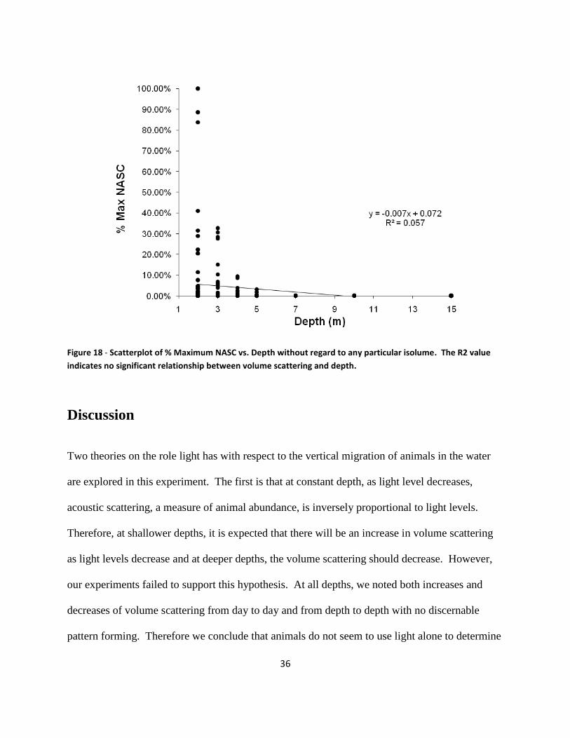
Figure 18 - Scatterplot of % Maximum NASC vs. Depth without regard to any particular isolume ........... 36

6

Introduction

Managers of marine and coastal resources are facing serious challenges. Examples of some of

these challenges include the over-exploitation of many marine species, the destruction of

important marine habitats, ocean pollution, introduction of invasive species, and global warming

and climate change. On top of this, managers must meet multiple and even conflicting legal and

societal mandates for the sustainable use of ocean and coastal resources (Link 2002; Link et al.

2002; Slocombe 1998). Focusing on just one or two aspects or uses of the marine environment is

not enough (Francis et al. 2007). The complexity of marine ecosystems necessitates a much

broader approach to ocean management such as Ecosystem Based Management (EBM) which

has become a high priority for managers (Link 2002; Pikitch et al. 2004).

There have been a number of reports from commissions published that embrace EBM as a

viable approach for managing our marine resources (PEW Oceans Commission, 2003. US

Commission on Ocean Policy, 2004; National Research Council, 1999; West Coast Governor‟s

Agreement on Ocean Health, 2008). For example, the West Coast Governors‟ Agreement on

Ocean Health suggests that ecosystem approaches to marine management go beyond single

species or single issue management. EBM for the oceans is the application of ecological

principles to manage key activities affecting the marine environment. EBM considers the inter-

dependence of all ecosystem components and the environments they live in (Levin and

Lubchenco 2008). An EBM approach provides a comprehensive understanding of the ecosystem

and is needed to support complex and difficult management systems (Slocombe 1998).

7

Meeting the goals and objectives outlined for EBM poses serious challenges for marine resource

managers. Application of EBM principles to marine resource management requires an

understanding of the interactions of organisms in a marine ecosystem and their surrounding

environment. They are complex, adaptive systems in which the interactions of small scale

components can have large influences in macrosystem dynamics which then feeds back to

influence the small scale systems (Levin 1998; Levin 2003; Levin and Lubchenco 2008).

Understanding the linkage among these scales and incorporating that knowledge into

management actions and policy decisions is paramount (Levin and Lubchenco 2008).

Developing an understanding of these linkages requires an immense amount of new information.

Experiments incorporating techniques such as the use of acoustical instruments to measure

abundance and migration patterns of pelagic animals can help scientists better understand these

complex linkages (Hewitt and Demer 2000; Holliday and Pieper 1995; Warren et al. 2001). The

research outlined in this study provides additional information about animal behavior that has

previously been unavailable. This study helps reveal more about the function and structure of

the marine ecosystem under conditions of low-light and at nighttime. This information can help

marine resource managers more clearly understand the role light plays in influencing the

nocturnal behavior of pelagic animals and provides data that has heretofore been missing.

Light plays an important role in a number of ecological processes in the ocean. For example,

light contributes to the oceans‟ temperature regime because light photons are absorbed by water

molecules and converted into heat (Lalli and Parsons 1993). More than one-half of the oxygen

in our air is generated by the photosynthesis process in the ocean (Reynolds 2006). Animal

behavior in the ocean can also be dependent on light. Vision is the primary means of prey

8

detection and feeding for many animals making foraging at low light levels difficult,

necessitating other adaptations for finding food. Prey often moves to lower light levels which

can be an active predator avoidance tactic (Abrahams and Kattenfeld 1997). Finally, light can

serve as a physiological cue for processes such as Diel Vertical Migration (Lalli and Parsons

1993).

Measurement of light levels in the ocean has focused primarily on Photosynthetically Active

Radiation or PAR. PAR is the amount of light available for photosynthesis (Hall 1999). Because

light is scattered and absorbed as it penetrates the ocean, there is an exponential decrease in light

intensity with increasing water depth, decreasing phytoplankton photosynthetic ability as well.

Consequently the maximum depth distribution of phytoplankton is controlled largely by the

intensity of light at depth or PAR (Lalli and Parsons 1993). Measurement of PAR during the day

is useful to develop a thorough understanding of the photosynthetic processes in the ocean and

their effects on our environment.

At night, instead of light being primarily used for photosynthesis, what little light is available

from the stars and moon is used for vision. Animals use the available light for predator detection

and avoidance as well as feeding (Han and Strakraba 2001). In many parts of the world ocean, a

migration of marine animals occurs towards the surface each night. This movement of animals

both large and small, called Diel Vertical Migration (DVM) (Gabriel 1988), is hypothesized to

be a response to the changing light levels after sunset which allows them to feed in rich surface

waters while avoiding predation by visual predators. Figure 1 is a cartoon showing the concept

of Diel Vertical Migration. The vertical axis represents depth in the ocean and the horizontal

axis represents different light periods of a day. Under daylight conditions, animals suspend

9

themselves in deeper water where light levels are low enough to avoid predation (Lampert 1989).

As the sun sets, surface light levels decrease and animals begin to move up towards the surface

to feed on food particles in the shallower depths (Han and Strakraba 2001; Van Gool and

Ringelberg 1997). They stay near the surface to feed during the night and if there is a moon rise,

they might drop down a little as surface light levels increase. Finally, as the sun rises the next

morning, the animals drop down to deeper water where light levels are low to avoid their

predators again.

Figure 1 – Mechanics of Diel Vertical Migration

10

Some researchers have suggested that animals accomplish this balance of minimizing the risk of

detection by predators while maximizing their opportunities for feeding by remaining at a

constant light level, or isolume (Roe 1983; Widder and Frank 2001). As light levels vary during

the night, the depth of the isolume moves up and down. Animals are hypothesized to adjust their

location in the water column accordingly to maintain optimal benefits. However, little work has

been done to test this theory. Widder and Frank (2001) used a low light auto-radiometer

(LoLAR) in a submersible to gather light level readings at different depths. The depth of the

submersible was adjusted to keep the light input into the LoLAR as constant as possible. Their

primary goal was to measure the speed of the isolume as it moves vertically in the water. No real

analysis of animal abundance along the isolume was done. They made estimates of animal

distribution by running visual transects during the day but were not able to gather abundance

data at night. Therefore, no conclusion of the relationship of animal movement and light levels

were made (Widder and Frank 2001).

While relatively inexpensive, off the shelf instruments are available to measure PAR during the

day, efforts to quantify light levels at night have proven more difficult. This is primarily because

the light levels at night are too low to be detected by standard radiometers. The goal of this work

was to quantify nighttime light levels while simultaneously examining the movement of pelagic

animals to explore the role light plays in the vertical movement of these animals during

crepuscular periods and during the rise and set of the moon. There have been few studies to

explore animal movement as light conditions change and none have involved using bioacoustical

measurement of animal abundance and in-situ light level readings. For example, Nelson, et al.

acoustically tracked the movement of a megamouth shark off the coast of California in 1990

during crepuscular periods. Acoustical transmitters were used to track the shark. Their light

11

data were not taken real-time. Isolume data were constructed from twilight illumination profiles

and then adjusted for depth using a seawater light extinction coefficient (Nelson 1997).

However, Widder and Frank (2001) point out that to do accurate analysis of the relationship of

animal movement in the water and isolumes, in-situ light data is essential. Hernandez, et al.

(2001) looked at zooplankton abundance in subtropical waters and tried to correlate those data to

lunar cycles. Their abundance information came from historical zooplankton abundance data

taken from bi-monthly samples at an oceanic station. Animal samples were taken from oblique

tows from 200 m up to the surface. This experiment did not collect any light data for analysis of

any relationship between abundance or movement of animals and changing light conditions.

They only looked at data from phase changes of the moon (Hernández-León 2001). Finally,

Ashjian, et al. (2002) looked at the distribution, annual cycles, and vertical migration of

acoustically derived biomass in the Arabian Sea. Estimates of biomass were made using data

from deployment of an acoustic Doppler current profiler (ADCP) made over a period of ten

cruises along a 1000 km transect. No real-time acoustical biomass data were collected. This

experiment also did not collect any in-situ light level data or attempt to correlate distribution or

movement of animals in the water to light (Ashjian 2002).

The difference between these few studies and the work presented here is that in this study, light

levels are quantified at the surface and down through the water column while simultaneously

measuring the vertical movement of mysids and zooplankton using acoustical instruments. This

study was performed in shallow water in Monterey Bay, California during May 2008. Of

particular interest was analysis of Diel Vertical Migration of zooplankton and mysids due to

benthic emergence. Using the quantified light and animal movement data two hypotheses are

tested:

12

1. At a constant depth, light can be used to predict animal abundance.

2. Animals follow an isolume as it moves vertically in the water column.

13

Methods

Field Site

Data for this analysis was collected during a scientific cruise in May 2008 in the Monterey Bay

National Marine Sanctuary (MBNMS) in Northern California. The MBNMS is the nation‟s

largest Marine Sanctuary, encompassing approximately 350 miles of California coastline

extending from San Francisco Bay in the north to approximately 100 miles south of Monterey

Bay. The sanctuary waters host a variety of diverse habitats from lush kelp forests to productive

coastal lagoons to deep sea communities in water over 3000 meters deep. A combination of

geological and oceanographic characteristics in the sanctuary contributes to providing highly

nutrient rich waters within the sanctuary boundaries. Because of the high concentration of

nutrients in the water this area is rich with animal life and contains some of the greatest

biodiversity in the temperate regions of the earth. Other habitats outside the sanctuary

boundaries are also linked to the MBNMS and are critical for migrating species that frequent the

area (http://montereybay.noaa.gov/).

During the period from May 17 to May 27, 2008 a scientific cruise on the 16 m R/V Shana Rae

was undertaken in Monterey Bay National Marine Sanctuary (MBNMS) to collect data on light

levels and acoustical backscatter from pelagic animals. The general data collection area was

chosen because of the high water column productivity observed during previous experiments

(Benoit-Bird, unpublished data) and was somewhat protected from strong winds from the

northwest. Sampling occurred between 2 and 6 km from shore in shallow water from 15 to 25

meters deep. Figure 2 is a site map of the experiment area in the Monterey Bay National Marine

14

Sanctuary. Stationary experiment sites are labeled as Sun-Moon Stations 1-6 and are shown as

orange dots on the site map. Transect grids were followed from stations A1-A5 and G5-G1. The

individual station sites shown are CTD sampling sites performed on the transect grids.

Figure 2 - Site map of project experiment area in Monterey Bay, California. Stationary stations are labeled as

Sun-moon Stations 1-6 and shown as orange dots. Transect grids were performed from stations A1-A5 and G5-

G1. CTD sampling was performed at individual station sampling sites.

Data Collection

Data were collected from approximately two hours before sunset until about 6 hours after sunset

each day. During 6 nights, data were collected at one of the four stationary sites shown by the

orange dots. On 2 other nights, sampling was conducted over a predefined transect grid. During

all sampling, a SBE19 plus CTD was deployed at half hour intervals to gather temperature,

salinity, and depth data. The CTD was also equipped with a WetLabs C-Star transmissometer

(25 cm path length, 530 nm wavelength), to gather information on light transmissivity in the

15

water column. Every hour, a vertical plankton net tow with a 0.75 m diameter, 333 m mesh net

equipped with a General Oceanics flowmeter was made to gather samples of animals.

Acoustic Measurements

The movement of pelagic animals up and down the water column was tracked by recording the

acoustical backscatter of the animals using a calibrated, split-beam, four-frequency echosounder

system (SIMRAD EK 60 at 38, 70, 120 and 200 kHz). The echosounder transducers were

mounted 1 m below the surface on a flat plate attached to a rigid vertical pole secured to the side

of the ship. The 38 kHz echosounder had a 12º conical beam. The 70 kHz echosounder had a 7º

conical beam. The 120 and 200 kHz echosounders each had a 7º conical beam. All four

frequencies used a 256µs pulse resulting in a vertical resolution of 10 cm. The echosounders

were calibrated in the field following the procedures outlined by Foote et al. (1987).

Acoustic Data Analysis

Acoustic backscatter data collected on the echosounder system were processed with Myriax‟s

Echoview software. Shown in Figure 3 is a plot of the data collected by the 120 kHz

Echosounder on May 21, 2008. This plot, or echogram, shows the depth of the water column on

the vertical axis ranging from the surface to the bottom which was 15 meters at this site. The

horizontal axis displays the time span of this echogram which is 6 hours. The colors shown on

the echogram are indicative of the strength of the backscatter signal received by the echosounder

from animals in the water. The color bar on the right of the figure shows the relative differences

in signal strength with the browns and reds having the highest backscatter levels and the blue and

gray colors showing weaker backscatter signal strength. The metric used on the color bar is

Scattering Volume, or Sv. It is a logarithmic measure of volume backscatter. The metric used in

this analysis is Nautical Area Scattering Coefficient or NASC. NASC is a linear measure of

16

backscatter and is proportional to animal abundance. NASC is measured in units of m2/nmi

2.

See Maclennen et al. (2002) for more details on the derivation and measurement of NASC.

Further examination of Figure 3 shows strong signal returns in the surface waters. These signals,

indicated by brown color, are caused by noise bubbles and/or fish near the surface. Because of

this strong noise layer, analysis of animal movement in this experiment was done starting at

depths below 2 meters. The blue patches (circled in red) are signal returns from zooplankton.

Note that there are areas of marked vertical movement towards the surface as indicated by the

arrows on the echogram. Near the far lower right of the echogram we can see emergence of

benthic animals (circled in green) that have emerged from the sediment layer.

Figure 3 – Echogram of 120 kHz Echosounder data taken on May 21, 2008

17

Data collected during these six nights were analyzed to explore what relationship there might be

between volume backscattering and light levels. Backscatter data analysis was done by creating

1 meter vertical by 1 minute horizontal bins and integrating the NASC within each bin. The

integrated values are proportional to the animal abundance in each bin area. Data were separated

into discrete depth levels ranging from 2 to 15 meters below the echosounders. The light and

volume backscatter data collected were used to test two separate hypotheses:

1. At a constant depth, the total acoustic backscatter, which is a measure of animal biomass

in the water, would be inversely proportional to light level.

2. Animal biomass will remain constant at a constant light level or isolume, even as the

isolume moves vertically in the water column.

To analyze relationships between illumination levels and animal abundance at constant depths,

NASC was examined as a function of illumination to determine if animal abundance varied

inversely with light levels. To test for significance in the correlation between light levels and

volume backscatter over the sampling period, data were scaled to a percentage of maximum

NASC and percentage of maximum illumination from a specific depth. Scaling of the data was

done to eliminate differences in magnitudes of NASC and light level between days and depths.

A regression analysis was performed on the data.

To see if animals follow an isolume vertically in the water column, a band of +/- one meter depth

around the isolume was established. Averaged values of volume backscatter within the +/- one

meter band were calculated and plotted as a function of time along with the isolume to see how

the volume backscatter varied along that isolume. Scatter plots were also generated to explore

18

the relation between NASC and depth of an isolume and the relation between NASC and depth

without regard to any isolume. Scaled percentages of maximum NASC and percentages of

minimum depth were used to eliminate differences in the magnitudes of NASC and depth

between days. In each case, regression analysis was then performed.

Light Level Measurements

The measurement of surface light level intensity and changes was done using custom, very

sensitive light sensors. These measurements were coupled with profiles of light attenuation

down through the water column from the transmissometer to develop a profile of light level in

the water column.

Light Measurement

A custom light sensor, called the Nightlight, was developed for recording extremely low light

levels during the night (Wisdom and Benoit-Bird 2008 (in review) Appendix 1). Four Nightlight

sensors were used during this cruise and were mounted in the “crow‟s nest” or top of the mast of

the R/V Shana Rae. The top of the mast location was used because it provided a mounting

location that was minimally affected by the operation and running lights of the ship. A previous

deployment of the Nightlight sensors where there was interaction with ship operation lights

showed the critical importance of proper Nightlight sensor placement (Wisdom and Benoit-Bird

2008 (in review) Appendix 1). The Nightlight sensor contains a datalogger and stores the output

of a photodiode that measures the light level. These instruments were calibrated by Wisdom and

Benoit-Bird (in review) to provide absolute light levels at the surface of the ocean. The

dataloggers were programmed to start recording light level data approximately two hours before

19

sunset and to stop recording data two hours after sunrise the next morning.

To determine light levels down through the water column, measurements of the transmission of

light through the water column were needed. The transmissometer used here measured light

attenuation at 530 nm, the peak sensitivity of the light measured by the Nightlight and near a

peak of the spectrum of nocturnal light (Johnsen 2006). Integrated into the CTD, the

transmissometer was lowered down into the water every one-half hour during each evening of

the cruise, providing data on the transmissivity and depth 8 times a second as it transversed from

the surface to near the bottom and back.

Light Data Analysis

To explore what correlation there might be between light and vertical movement of pelagic

animals in the ocean, one must be able to measure the levels of light intensity during sampling

periods. Measurement of light during the day is relatively easy. A radiometer is used to make

daytime light measurements. It measures irradiance in standard wavelengths from 400 to 865

nm. Sensitivity for this type of instrument ranges from 300 to 2.5 E-03 µwatts/cm2.

Unfortunately, radiometers intended for use during the day are not sensitive enough for

measurement of light levels during crepuscular periods or nighttime. Kaul, et al.(1994)

measured the available light on a cloudless, moonless night to be as small as 9.6 *10-5

µwatts/cm2. To overcome this problem, a custom, very sensitive light sensor was developed

called the Nightlight (Wisdom, Benoit-Bird 2008 (in review) Appendix 1). This sensor is

simple, inexpensive, easy to operate, and is very sensitive. The measured sensitivity range of a

typical Nightlight sensor is from 12 to 1.7 x10-9

µwatts/cm2.

20

Figure 4 shows the calibrated data from a typical Nightlight sensor collected in Monterey Bay on

May 21, 2008 over the time period from 1800 to 0030 local time the following morning. Sunset

was around 2120 and moonrise was around 2215 local time as shown by the red lines in the plot..

Figure 4 – Typical plot of Nightlight Sensor output (µwatts/cm2)

Figure 5 is the same data but with the Y axis converted to a log scale to show the variability of

the light sensor output more clearly.

21

Figure 5 – Log Plot of Nightlight Sensor output illustrating the variability of Nightlight Sensor output

Using the surface light levels recorded by the Nightlight sensor at the exact times the

transmissometer was deployed, profiles of the light levels down the water column can be

developed. Figure 6 shows plots of transmissivity data and light levels down the water column

for data collected on May 21. The left plot shows light transmission as a percentage and the

right plot is illumination versus depth in meters. Transmissivity is measured as a percent and

represents the amount of light penetration down through the water column. Illumination is

measured as µwatts/cm2. The surface light level recorded by the Nightlight sensor can then be

applied to the transmissivity data and the result is a plot of the decay of light levels as water

depth increases. As can be seen, the illumination levels drop off quickly from the surface to

22

approximately three meters in depth and more slowly as depth increases as shown by the right

plot in Figure 6.

Figure 6 - Plots of transmissivity percentage and light levels in water column vs. depth. Light levels drop off

dramatically from the surface to approximately 3 meters in depth.

To see how the depth of constant light level varies over time, depth data throughout an

experiment period for a constant light level were plotted. Figure 7 shows the variance of the

depth of a constant light level of 0.01 µwatt/cm2 throughout the night of May 20, 2008. This plot

of constant illumination varying over time and/or depth is called an isolume. The vertical axis

shows the depth of the isolume in meters and the horizontal axis is the time the transmissivity

readings were taken that evening. On this day, sunset was at 2012 local time and moon rise was

at 2121 local time as indicated by the vertical red lines in Figure 7. Looking at the plot we can

see how the isolume depth decreases as the sun sets and it increases as light levels increase with

23

the moonrise. Note that it takes a few minutes for the isolume to begin moving into deeper

water. The reason is that the moon has to rise above the horizon somewhat to begin having an

effect on the isolume.

Figure 7 - Plot of 0.01 µwatt/cm2 isolume on 20 May, 2008. The vertical red lines indicate the time of sunset and

moonrise. Note the lag time before the depth of the isolume increases due to the time required for the moon to

raise high enough to have an effect on surface light levels.

24

Results and Discussion

Hamner describes Diel Vertical Migration or DVM as perhaps the most massive animal

migration on the planet (Hamner 1988). It has been suggested that animal distribution patterns in

the ocean can be affected by light (Widder and Frank 2001). There are two popular hypotheses

about the role light may play in vertical migration of animals in the ocean. One is the “rate of

change” theory. It suggests that animal migration might be affected by light intensity change

and/or direction of change (Clarke 1930; Ringelberg 1964). The other is the “preference” theory.

It suggests that animals prefer certain light levels or zones and will follow those zones up and

down the water column as the amount of light available varies with depth (Russell 1926; Roe

1983; Widder and Frank 2001).

The first hypothesis tested in this experiment is that at a constant depth, the total acoustic

backscattering, a measure of the biomass of animals in the water, would be inversely

proportional to light level. To test this hypothesis, volume scattering and light level data were

collected during a scientific cruise in Monterey Bay National Marine Sanctuary in May, 2008.

Contrary to our expectations, we found no predictable pattern in the relationship between light

level and acoustic backscatter signal. Figure 8 is an example of data collected during the

evening of May 19. Plotted on the vertical axis is Nautical Area Scattering Coefficient or NASC

in units of m2/nmi

2 at a depth of three meters. The dots on the plot are estimates of animal

abundance derived by integrating data from the echosounder in 1 meter depth by 1 minute time

bins. The resultant value is the estimated animal abundance in that area or NASC. Plotted on

25

the horizontal axis is the light level present at a depth of 3 meters at various times during the

night when transmissivity data were collected from CTD deployment. The illumination values

were calculated using data from the Nightlight sensor coupled with measures of the water

column transmissivity. In this case, as light levels decrease, volume scatter increases which

would be expected if animals do migrate upwards towards the surface as light levels decrease.

Figure 8 – Nautical Area Scattering Coefficient (NASC (m2/nmi

2)) vs. Illumination (µwatts/cm

2) at a depth of 3

meters on May 19. The dots on the plot are estimates of animal abundance derived by integrating data from

the echosounder in 1 meter depth by 1 minute time bins. The plot shows NASC or volume scattering increasing

as light levels decrease.

Figure 9 is a plot of data taken at three meters depth on May 20. Interestingly, this plot shows

the volume scattering decreasing as the light levels decrease. This pattern is contrary to what the

26

prevailing theory suggests: that animals should migrate upwards at low light levels, resulting in

an increase in volume scattering at shallow depths as light levels decrease.

Figure 9 - Nautical Area Scattering Coefficient (NASC (m2/nmi

2)) vs. Illumination (µwatts/cm

2) at a depth of 3

meters on May 20. The dots on the plot are estimates of animal abundance derived by integrating data from

the echosounder in 1 meter depth by 1 minute time bins. The plot shows NASC or volume scattering decreasing

as light levels decrease.

The same analysis was done for a depth of fifteen meters. Figure 10 is a plot of volume

scattering versus light levels at a constant depth of fifteen meters for data collected on May 26.

Volume scattering decreases as light levels decrease which seems logical if animals migrate to

27

the surface as light levels decrease. If animals migrate towards the surface the abundance should

decrease in deeper water levels.

Figure 10 - Nautical Area Scattering Coefficient (NASC (m2/nmi

2)) vs. Illumination (µwatts/cm

2) at a depth of 15

meters on May 26. The dots on the plot are estimates of animal abundance derived by integrating data from

the echosounder in 1 meter depth by 1 minute time bins. The plot shows NASC or volume scattering decreasing

as light levels decrease.

On the other hand, data shown in Figure 11 for a fifteen meter depth on May 17 illustrates just

the opposite: In this case we can see an increasing trend in volume scattering as light levels

decrease which is again contrary to what one would expect.

28

Figure 11 - Nautical Area Scattering Coefficient (NASC (m2/nmi

2)) vs. Illumination (µwatts/cm

2) at a depth of 15

meters on May 17. The dots on the plot are estimates of animal abundance derived by integrating data from

the echosounder in 1 meter depth by 1 minute time bins. The plot shows NASC or volume scattering increasing

as light levels decrease.

Examination of the rest of the data from other days and other depths showed these same

contradictions. On a given day, some depths showed increases in volume scattering as light

levels decreased and other depths showed decreases in volume scattering.

To determine if there was any significant relationship between the light levels and volume

scattering over the sampling period, the data from each day were scaled into percent of

maximum NASC and percent of maximum illumination from that depth during that day in order

to eliminate differences in the magnitudes of NASC and light levels between days and depths.

Figures 12 and 13 are scatter plots of data taken for all six days at a constant depth of three

29

meters and fifteen meters, respectively. Linear Analysis indicates that there is no significant

relationship between light levels and volume scattering at constant depth. Based on this data set,

we can conclude that light alone is not a significant predictor of the volume scattering, a measure

of animal biomass, present at a constant depth in this area of Monterey Bay. The migration

patterns recorded for a particular depth were not consistent. Some days showed an upward

movement, some depicted downward movement and others showed no dramatic movement at

all. This suggests that this particular area experiences some upward vertical migration, some

downward or reverse vertical migration, and perhaps some horizontal migration or advection of

animals during each evening.

Figure 12 – Scatterplot of % Maximum NASC vs. % Maximum Illumination at constant 3 meters depth for data

collected on all six days of the experiment. Low R2 value indicates that there is no significant relationship

between volume scattering and light levels at a constant depth.

30

Figure 13 - Scatterplot of % Maximum NASC vs. % Maximum Illumination at constant 15 meters depth for data

collected on all six days of the experiment. Low R2 value indicates that there is no significant relationship

between volume scattering and light levels at a constant depth.

The second hypothesis tested in this experiment is that animals follow an isolume. If the theory

that animals attempt to remain at a constant light level is true, it can be hypothesized that animal

biomass measured as NASC will remain constant at a constant light level or isolume, even as this

isolume moves vertically in the water column. Contrary to our predictions, we found that

animals do not simply follow isolumes and that there is no significant relationship between

animal volume scattering and depth. Figure 14 shows the variability of the depth of the 0.1

µwatt/cm2 isolume over time taken on May 17, 2008. In this instance, light data were collected

31

starting two hours before sunset and continued throughout the night. On this evening sunset was

at 2012 local time. The plot shows the movement of this isolume towards the surface as surface

light levels diminish. Around 2130 we see the direction of the isolumes vertical movement

change as a result of the rise of a nearly full moon at 2121 local time.

Figure 14 – Plot of 0.1 µwatt/cm2 isolume on 17 May, 2008

To test the hypothesis that animals follow an isolume, a +/- 1 m band around the isolume was

created as shown in Figure 15. Average values of volume backscatter within the +/- 1 meter

band were calculated and plotted as a function of time to estimate the variance of volume

scattering about the 0.1 µwatt/cm2 isolume. If the animals prefer to remain at an isolume as

hypothesized, one would expect a relatively constant amount of volume backscatter over the

32

entire evening. Figure 16 shows two curves; a constant level of animal abundance (solid black

line) as would be expected if animals follow an isolume and the actual animal abundance

(dashed red line) calculated by averaging the NASC values within the +/- 1 meter band around

the isolume. The plot shows that there is wide variation of animal abundance around the isolume

instead of being constant as predicted. Individual isolume plots along with volume scattering

data were made for a number of light levels and days. Each plot showed the same wide variation

in animal abundance we see in Figure 16. The results indicate that the amount of volume

backscatter varies considerably along an isolume rather than being relatively constant so it is

concluded that animals are not simply following an isolume up and down the water column.

Figure 15 - Plot of +/- 1 meter band around the 0.01 µwatt/cm2 isolume of May 17, 2008

33

Figure 16 – Plot of predicted constant level of animal abundance (black) and actual averaged volume backscatter

or NASC (dashed red) calculated +/- 1 meter about the isolume. Plot shows considerable variability of volume

scattering along an isolume instead of being relatively constant.

While there does not appear to be any relationship between volume backscatter and the isolume,

there might be a relationship between volume backscatter and the depth of isolumes. To test this,

the percent of maximum NASC was plotted as a function of the percent of minimum isolume

depth for all data collected for the following isolumes: 1, 0.1, 0.01, 0.001, 0.0001, 1x10-5

, and

1x10-6

µwatt/cm2. The NASC and depth numbers were scaled to a percentage of the maximum

NASC and minimum depth values recorded for each day to eliminate differences of variances of

NASC and depths between different isolumes and days. The results are shown in Figure 17. A

linear trend line and the R2 value are shown on the plot. The R

2 value of 0.242 indicates that

there might be a relationship between volume backscatter and the depth of the isolume. An

34

exponential curve was also fitted to the data and an R2 value of .311 was calculated. The relative

difference in goodness of fit (R2 values) did not change significantly using exponential

regression compared to linear regression, suggesting that the pattern shown in the figure is

robust.

To test if this effect was simply related to the depth rather than the depth of the isolumes, the

relationship between the percentage of maximum NASC each night as a function depth for data

taken at 2,3,4,5,7,10, and 15 meters . The results are shown in Figure 18. The small R2

value of

0.057 indicates that there is no significant relationship between volume backscatter and depth.

An exponential curve was also fitted to the data and an R2 value of .147 was calculated. The

relative difference in goodness of fit (R2 values) did not change significantly using exponential

regression compared to linear regression, suggesting that the pattern shown in the figure is

robust. The relationship observed in Figure 18 is not simply a response of the acoustic scatterers

to depth, but to the interaction of in-situ light levels and depth.

35

Figure 17 – Scatterplot of % Maximum NASC vs. % Minimum Depth along isolume depths. The R2 value indicates

there might be a relationship between volume scattering and depth of an isolume.

36

Figure 18 - Scatterplot of % Maximum NASC vs. Depth without regard to any particular isolume. The R2 value

indicates no significant relationship between volume scattering and depth.

Discussion

Two theories on the role light has with respect to the vertical migration of animals in the water

are explored in this experiment. The first is that at constant depth, as light level decreases,

acoustic scattering, a measure of animal abundance, is inversely proportional to light levels.

Therefore, at shallower depths, it is expected that there will be an increase in volume scattering

as light levels decrease and at deeper depths, the volume scattering should decrease. However,

our experiments failed to support this hypothesis. At all depths, we noted both increases and

decreases of volume scattering from day to day and from depth to depth with no discernable

pattern forming. Therefore we conclude that animals do not seem to use light alone to determine

37

their position in the water column and that light is not a significant predictor of the amount of

volume backscattering at constant depth.

The second theory is that animals follow an isolume up and down the water column as light

levels change. Individual isolume plots along with volume scattering data showed scatter

volume varying widely along an isolume rather than being fairly constant as one would expect if

animals followed an isolume. Additional analysis showed that there may be a relationship

between volume backscattering and depth along a specific isolume but no relationship between

volume backscatter and depth in general. The implication of these findings is that animals do not

simply follow an isolume up and down the water column as light levels vary. There is no

significant relationship between depth and animal volume scattering and that vertical migration

of pelagic animals is a much more complex relationship that involves the interaction of both light

and depth.

There are some things that should be pointed out that may impact the results of this study. First,

there is some inherent heterogeneity in the data. One cause is the result of a long sampling

period of transmissivity data. The transmissivity data were collected on ½ hour intervals.

Consequently, illumination data used in the analysis were not continuous over time. The effect

of this is that we are looking at light level changes at ½ hour increments instead of being

continuous. Also, the animal abundance data used were those values recorded at the time the

transmissivity data were collected. This results in fewer data points being available for analysis.

An alternative to this approach would be to analyze all transmissivity data collected during one

night time series and see how much the transmissivity varies. If there is not much variation

during the evening, then a general profile of transmissivity down the water column for that night

38

could be derived and applied throughout the night resulting in having many more data points

available for analysis. Another potential cause of data heterogeneity is animal patchiness in the

water. The boat was drifting with the current and wind and could move over a patch of

zooplankton quickly which may affect animal volume scattering numbers. In addition,

horizontal advection of zooplankton may affect volume scattering as the animals move through

the study area.

A second issue is the effect of ship running/operation lights at night. One problem is that bright

lights around a boat do attract many marine animals towards the surface. Care must be taken to

remove the effects of extraneous light as much as possible during nighttime studies to avoid

artificial increases of animals in water near the surface. During this study, extreme care was

taken to eliminate all effects of ship operation/running lights during data collection periods.

Another issue is that the Nightlight Sensors are extremely sensitive and recorded light data can

be affected adversely by even the slightest addition of artificial light. In this study, the sensors

were mounted on the mast of the ship inside the “crow‟s nest” to eliminate any affects ship lights

might have. In addition, only flashlights were used on deck while collecting data. These

precautions insured that light data recorded by Nightlight Sensors were only from nocturnal light

and not from the ship.

Finally, this was a shallow water study to analyze vertical migration of mysids and zooplankton

due to benthic emergence. The results presented in this study are specific to the shallow waters

in this ecosystem. It is not known how these results might be transferred to marine ecosystems

in other parts of the world.

39

Implications for Monterey Bay National Marine Sanctuary

Managers

The West Coast Governors‟ Agreement on Ocean Health, the US Commission on Ocean Policy

and the PEW Oceans Commission recommend the principles of Ecosystem Based Management

(EBM) be used as guidelines for managers of marine resources (PEW Oceans Commission,

2003; US Commission on Ocean Policy, 2004; West Coast Governor‟s Agreement on Ocean

Health, 2008). Marine resource managers other than those responsible for marine sanctuaries are

not yet mandated to use EBM principles but many are integrating them into their management

strategies. Managers of marine sanctuaries such as the Monterey Bay National Marine

Sanctuary, however, are mandated to use EBM principles in managing the nation‟s marine

sanctuaries by the National Marine Sanctuary Act (NMSA) (16 U.S.C. 1431)

(http://sanctuaries.noaa.gov/about/legislation/). Two important goals of the NMSA include:

1. Maintain the biological communities in national marine sanctuaries, to protect and restore

and enhance habitats, population and ecological habitats.

2. Support, promote, and coordinate scientific research on, and long-term monitoring of, the

resources of the marine areas.

In response to the EBM mandate the managers of the Monterey Bay National Marine Sanctuary

(MBNMS) adopted a Sanctuary Action/Management Plan and Environmental Impact Statement

(http://sanctuaries.noaa.gov/jointplan/fmp/101408mbnmsfmp.pdf). Two key areas of emphasis

for Sanctuary Mangers are the protection of Sanctuary resources and marine research. The

40

Sanctuary Action/Management Plan identifies a number of key strategies to be implemented to

address these areas (http://montereybay.noaa.gov/intro/mbnms_eis/). A scientific research

framework has been established outlining three types of scientific studies that are essential to

implementing the Action/Management Plan strategies

(http://montereybay.noaa.gov/intro/mbnms_eis/):

Baseline Studies – Studies that are designed to obtain an understanding of the ecology of

the Sanctuary at present.

Monitoring Studies – Monitor Sanctuary data over longer periods and use this data to

make adjustments to management policies and/or adapt to changing conditions as they

occur.

Predictive Studies – Analysis of causes and consequences of ecosystem changes that are

more short-term in nature and are intended to address immediate management issues.

The stated highest priority of the Sanctuary is to “protect its marine environment, resources

and qualities”. A key part of this objective is to ensure that research results and scientific

data collected from the marine sanctuary are utilized by appropriate management agencies in

their resource protection strategies. Managers realize that scientific investigations and

research into Monterey Bay ecosystem structures and functions are essential.

The acoustical study collecting data on pelagic animal abundance and behavior presented

here can help Sanctuary Managers meet these goals. While light has been identified as

playing a role in the behavior of marine animals at nighttime (Widder and Frank 2001), no

data has been available that correlates nocturnal behavior of pelagic animals with changing

41

low-light conditions. Integrating information about the structure and function of the marine

ecosystem under conditions of low-light and at nighttime, as outlined here, provides

information about ecosystem processes which has been largely unavailable. Following are

some specific examples of how MBNMS managers can be informed by the data presented.

Predator/prey interaction – Monterey Bay is an important stop-over for migrating Grey Whales

(Pelagic Working Group 2002; Forney 2007). They rely on mysids, a type of zooplankton, and

herring/sardine populations for food (Pauly et al. 1998, Darling 1998). Typically, mysids,

sardines, and herring congregate and feed on plankton in surface waters at night (Nilsson 2003,

Mackinson 1999). A fluctuation in the abundance of prey animals or a change in prey migration

patterns could impact the distribution and residence patterns of migrating whales in the

Sanctuary as well as their overall health. Our results show that in the Northeast corner of

Monterey Bay, there is no clear diel benthic emergence pattern of mysids. Our data suggest a

much more complicated pattern of near bottom scatterers in response to time of day, depth, and

light. This provides baseline data describing the nocturnal behavior of mysids and other pelagic

animals in this part of Monterey Bay. Using the techniques outlined in this project, baseline data

for other areas of Monterey Bay could also be obtained and compared with periodic monitoring

studies to look for changes or alterations of nocturnal prey behavior that might affect the health

of the prey populations and ultimately the health of the migrating whales. This knowledge could

enable managers to adjust their Grey Whale management plans in the Sanctuary accordingly, for

example reducing boat traffic or limiting fishing effort in key prey areas during grey whale

residence.

42

Schooling Pelagic Fishery – The night fishery for pelagic schooling fish (sardines, anchovies,

and herring) in Monterey and San Francisco Bays are the northernmost sardine fishing centers in

California. Schools of Pacific Herring that move into the state's northern bays to spawn provide

an important food source for other animals including invertebrates, fish, birds and mammals

http://www.dfg.ca.gov/marine/herring/oc_article.asp. Herring in California have been harvested

primarily for their roe, with small amounts of whole herring marketed for human consumption,

aquarium food, and bait http://www.dfg.ca.gov/marine/status/pacific_herring.pdf. These fish

feed on plankton that resides in the bay (Cascorbi 2004). During nighttime, small animals

typically migrate towards the surface to feed. The herring and sardine schools follow and

congregate near the surface, feeding on the plankton and other small animals. This congregation

of sardine, anchovy, and herring schools makes the fish more catchable at night. Having access

to data on the nocturnal behavior of these small animals can help managers develop an

understanding of the location and distribution of these schooling pelagic fish at night and obtain

an estimate of the abundance of the food sources for these fish. Shifts in abundance or migration

patterns of the plankton food source could be an indicator of pending problems or changes with

this fishery. Using this information, managers can make predictions about the effects on this

fishery and can alter their management strategies as necessary.

Changes in relative distribution – Changes in animal density or distribution can be an indicator

of some sort of perturbation in the marine ecosystem. Natural phenomena such as Sea Surface

Temperature change or an ENSO (El Niño – Southern Oscillation) event are known to alter

oceanic characteristics and can affect the behavior of animals in the water (Crocker et al. 2006;

Ottersen et al. 2001; Trillmich and Limberger 1985). Changes in the nocturnal migration

pattern or distribution/abundance shifts can alert Sanctuary managers of potential problems.

43

This data can help them determine the locale and extent of the perturbation and provide valuable

data for modeling the effects to Sanctuary waters.

Studies of the health of whales, pinnepeds and seabirds in the Sanctuary – The health of these

animals is of primary concern for Sanctuary Managers. Prey abundance and distribution studies

can help managers understand population changes in a particular sea mammal or sea bird.

Fluctuating abundance or changes in migration patterns of food sources could be essential

information to managers monitoring and protecting the health of these species providing

explanations for observed patterns or ruling out potential impacts. Nocturnal behavior studies of

the prey of animals like murres and sea lions that are known to feed at night on resources that are

often unavailable during the day would be especially invaluable by providing insight into night

predator/prey interaction that has not been available until now.

Marine Protected Areas (MPAs) - In addition to protecting Sanctuary resources and conducting

marine research, MBNMS managers must also manage the Sanctuary as a Marine Protected Area

(MPA). MPAs are an important conservation tool for marine resource managers. The World

Conservation Union (ICUN 1988) formally defines a MPA as “any area of inter-tidal or sub-tidal

terrain, together with its overlying water and associated flora, fauna, historical and cultural

features, which has been reserved by law or other effective means to protect part or all of the

enclosed environment” (http://cmsdata.iucn.org/downloads/wpamarinepoaen.pdf). Over the

years the term MPA has emerged as a commonly used term implying conservation of species and

communities (Allison et al. 1998). In 1999 the State of California approved the Marine Life

Protection Act (http://www.dfg.ca.gov/mlpa/) that mandates the state design and manage an

improved network of marine protected areas in state waters. The MBNMS responded to this

44

mandate by considering the addition of more MPAs within Sanctuary boundaries as a priority

issue to be addressed in its Marine Protected Areas Action Plan

(http://montereybay.noaa.gov/resourcepro/resmanissues/mpa.html). The overall goal of the

Sanctuary managers is to determine if the addition of more MPAs can play a role in conservation

and management of the marine resources in Sanctuary waters. To effectively do this, important

biological data will be critical in the design and location of additional MPAs in the Sanctuary.

For example, knowledge of consistent migration patterns could help define MPA boundaries.

Data collected in low-light conditions or at nighttime might reveal hot spots or areas where

animals are congregating and feeding at night but may not be in during the day. Those areas

could be important habitats for pelagic animals and should be considered for inclusion into the

boundaries of the MPA.

45

Conclusion

The purpose of this project was to quantify nighttime light levels while simultaneously

examining the movement of pelagic animals to explore the role light plays in the vertical

movement of these animals during crepuscular periods and during moon rise and setting events.

The quantization of extremely low levels of light at night was done using a custom, very

sensitive light sensor called the Nightlight. Surface light level data from Nightlight sensors were

used along with water column transmissivity data to develop profiles of light levels down the

water column for each day of the experiment. These light profiles along with animal volume

scattering or abundance data were then used to explore two hypotheses about the role light plays

in the vertical movement of pelagic animals.

The first hypothesis tested was that at constant depths, light levels can be used to predict the

amount of volume scattering or abundance of animals in the water. Analysis of volume

backscatter data versus illumination levels at constant depth revealed that there is no significant

relationship between light levels and volume scattering at constant depths, contrary to the

hypothesis. The second hypothesis tested was that animals follow an isolume up and down the

water column as light levels change. Individual isolume plots along with volume scattering data

showed the amount of scattering varying widely along an isolume instead of being fairly constant

as was expected if animals follow an isolume. Instead, a complex relationship between volume

scattering, light levels, and depth of isolumes exists. Additional analysis of volume scattering

and depth without regard to specific isolumes showed no significant relation between scattering

volume and depth.

46

Managers of Monterey Bay National Marine Sanctuary face many challenges. They are

mandated by the National Marine Sanctuary Act to manage the Sanctuary using Ecosystem-

Based Management principles. They must address multiple and even conflicting societal

mandates for the sustainable use of ocean and coastal resources. The complexity of marine

ecosystems necessitates a much broader approach to ocean management.

The response to these challenges was a Sanctuary Management and Action Plan by which

managers manage the MBNMS. Two key strategies of the Management/Action Plan are data

collection on oceanographic parameters of the Sanctuary and establishment of a monitoring

program to assess environmental changes as they occur due to natural and human causes. A

scientific research framework was developed to implement these important strategies. It consists

of three different types of studies: Baseline, Monitoring, and Predictive. All three studies will

require an immense amount of data from numerous sources. One key source could be acoustical

instruments that can provide information on the behavior and abundance of pelagic animals in

the Sanctuary. The work done on this project specifically provides additional information about

nocturnal animal behavior that has previously been unavailable in Monterey Bay and elsewhere.

The research helps reveal more about the function and structures of the marine ecosystem under

conditions of low-light and at nighttime. Having access to animal behavior and movement in

low-light conditions and at nighttime provides sanctuary managers with new data that can be

used to help determine if there are differences in animal distribution between day and nighttime

and if so, how those differences affect other animals in the Sanctuary. This information also

helps managers in MBNMS more clearly understand the role light plays in influencing the

nocturnal behavior or pelagic animals in Sanctuary waters.

47

References

Abrahams, M. V., and M. G. Kattenfeld. 1997. The role of turbidity as a constraint on predator-

prey interactions in aquatic environments. Behavioral Ecology and Sociobiology 40: 169-

174.

Allison, G. W., J. Lubchenco, and M. H. Carr. 1998. Marine Reserves are necessary but not

sufficient for marine conservation. Ecological Applications 8: 79-92.

Agardy, T. 2000. Information needs for marine protected areas: scientific and societal. Bulletin

of Marine Science 66: 875-888.

Ashjian, C. J., S. L. Smith, C. N. Flagg, and N. Idrisi 2002. Distribution, annual cycle, and

vertical migration of acoustically derived biomass in the Arabian Sea during 1994–1995.

Deep-Sea Research Part II 49: 2377-2402.

Bollens, S. M., and B. W. Frost. 1989. Predator-induced diel vertical migration in a planktonic

copepod. Journal of Plankton Research 11: 1047-1065.

Cascorbi, A. 2004. Seafood Watch Seafood Report - Sardines. 1: 1 - 19.

Clarke, G. L. 1930. Change of Phototropic and Geotropic Signs in Daphnia Induced by Changes

of Light Intensity. Journal of Experimental Biology 7: 109-131.

Crocker, D. E., D. P. Costa, B. J. Le Boeuf, P. M. Webb, D. S. Houser. 2006. Impact of El Niño

on the foraging behavior of female northern elephant seals. Marine Ecology Progress Series 309:

1-10

Darling, J. D., K. E. Keogh, T. E. Steeves 1998. Gray Whale (ESCHRICHTIUS ROBUSTUS)

Habitat Utilization and Prey Species off Vancouver Island, BC. Marine Mammal

Science14: 692-720

Flik, B. J. G., and J. Ringelberg. 1993. Influence of Food Availability on the Initiation of Diel

Vertical Migration(DVM) in Lake Maarsseveen. Ergebnisse der Limnologie ERLIA 6 39.

Foote, K.G., Vestnes, G., Maclennan, D.N., Simmonds, E.J., 1987. Calibration of acoustic

instruments for fish density estimation: A practical guide. International Council for the

Exploration of the Sea Cooperative Research Report 144, Copenhagen, p. 57.

48

Forward R. B. 1988. Diel vertical migration: zooplankton photobiology and behaviour.

Francis, R. C., M. A. Hixon, M. E. Clarke, S. A. Murawski, and S. Ralston. 2007. Ten

Commandments for Ecosystem-Based Fisheries Scientists. Fisheries 32.

Gabriel, W. A. T., Bernhard. 1988. Vertical Migration of Zooplankton as an Evolutionarily

Stable Strategy. The American Naturalist 132: 199-216.

Hall, D. O. 1999. Photosynthesis.

Hamner, W. M. 1988. Behavior of plankton and patch formation in pelagic ecosystems. Bulletin

of Marine Science 43: 752-757.

Han, B., and M. Strakraba. 2001. Control Mechanisms of Diel Vertical Migration: Theoretical

Assumptions. Journal of Theoretical Biology 210: 305-318.

Hernández-León, S., C. Almeida, L. Yebra, , J. Arístegui, M. L. Fernández de Puelles, and J.

García-Braun. 2001. Zooplankton abundance in subtropical waters: is there a lunar cycle?

Scientia Marina 65 (suppl. 1): 59-63.

Hewitt, R. P., and D. A. Demer. 2000. The use of acoustic sampling to estimate the dispersion

and abundance of euphausiids, with an emphasis on Antarctic krill, Euphausia superba.

Fisheries Research 47: 215-229.

Holliday, D. V., and R. E. Pieper. 1995. Bioacoustical oceanography at high frequencies. ICES

journal of Marine Science 52: 279-296.

Johnsen, S., A. Kelber, E. Warrant, A. M. Sweeney, E. A. Widder, R. L. Lee, J. Hernandez-

Andres. Crepuscular and nocturnal illumination and its effects on color perception by the

nocturnal hawkmoth Deilephila elpenor. Journal of Experimental Biology 209: 789-800.

Kaul, S. R. and others. 1994. Atmospheric extinction and background light measurements at

Jammora, Jammu.

Lalli, C. M., and T. R. Parsons. 1993. Biological Oceanography: An Introduction. Pergamon

Press.

Lampert, W. 1989. The Adaptive Significance of Diel Vertical Migration of Zooplankton.

Functional Ecology 3: 21-27.

49

Levin, S. A. 1998. Ecosystems and the Biosphere as Complex Adaptive Systems. Ecosystems 1:

431-436.

---. 2003. Complex adaptive systems: Exploring the known, the unknown and the unknowable.

BULLETIN-AMERICAN MATHEMATICAL SOCIETY 40: 3-20.

Levin, S. A., and J. Lubchenco. 2008. Resilience, Robustness, and Marine Ecosystem-based

Management. Bioscience 58: 27-32.

Link, J. S. 2002. What does ecosystem-based fisheries management mean. Fisheries 27: 18-21.

Link, J. S. and others. 2002. Marine ecosystem assessment in a fisheries management context.

Canadian Journal of Fisheries and Aquatic Sciences 59: 1429-1440.

Loose, C. J. A. D., Piotr. 1994. Trade-offs in Diel Vertical Migration by Zooplankton: The Costs

of Predator Avoidance. Ecology 75: 2255-2263.

Mackinson, S., L. Nottestad, S. Guenette, T. Pitcher, O. A. Misund, A. Ferno 1999. Cross-scale

observations on distribution and behavioural dynamics of ocean feeding Norwegian

spring-spawning herring (Clupea harengus L.) ICES Journal of Marine Science 56: 613-

626.

Maclennan, D. N., P. G. Fernandes, and J. Dalen. 2002. A consistent approach to definitions and

symbols in fisheries acoustics. ICES journal of Marine Science 59: 365.

National Research Council. 1999. Sustaining Marine Fisheries. Washington

(DC): National Academy Press.

Nelson, D. R., J. N. McKibben, W. R. Strong, C. G. Lowe, J. A. Sisneros, D. M. Schroeder, and

R. J. Lavenberg. 1997. An acoustic tracking of a megamouth shark, Megachasma

pelagios: a crepuscular vertical migratory. Environmental Biology of Fishes 49: 389-399.

Nilsson, L. A. F., U. H.Thygesen, B. Lundgren, B. F Nielsen, J. R Nielsen, J. E.Beyer 2003.

Vertical migration and dispersion of sprat (Sprattus sprattus) and herring (Clupea

harengus) schools at dusk in the Baltic Sea. Aquatic Living Resources 16: 317-324.

Ottersen, G. B. Planque, A. Belgrano, E. Post, P. C. Reid, N. C. Stenseth. 2001. Ecological

effects of the North Atlantic Oscillation. Oecologia 128: 1-14.

50

Patterson, H.M., M. Lindsey, and S.E. Swearer 2007. Use of sonar transects to improve

efficiency and reduce potential bias in visual surveys of reef fishes. Environmental

Biology of Fishes 78: 291-297.

Pauly, D., A. W. Trites, E.Capuli, and V. Christensen. 1998. Diet composition and trophic levels

of marine mammals. ICES Journal of Marine Science: 55: 467–481.

Pelagic Working Group (2002). Pelagic Predators, Prey and Processes: Exploring the Scientific

Basis for Offshore Marine Reserves. Proceedings of the First Pelagic Working Group

Workshop. January 17, 2002. Santa Cruz, CA.

Pew Oceans Commission. 2003. America‟s Living Oceans: Charting a Course

for Sea Change. Arlington (VA): Pew Oceans Commission.

Pikitch, E. K. and others. 2004. ECOLOGY: Ecosystem-Based Fishery Management, p. 346-

347. Science.

Reynolds, C. S. 2006. Ecology of Phytoplankton.

Ringelberg, J. 1964. The positively phototactic reaction of Daphnia magna Straus: A

contribution to the understanding of diurnal vertical migration. Neth. J. Sea Res 2: 19406.

Roe, H. S. J. 1983. Vertical distributions of euphausiids and fish in relation to light intensity in

the Northeastern Atlantic. Marine Biology 77: 287-298.

Russell, F.S. 1926. The vertical distribution of marine macro-plankton. IV. The apparent importance of light intensity as a controlling factor in the behavior of certain species in

the Plymouth area. J. Mar. Biol. Ass. UK 14: 415-440.

Slocombe, D. S. 1998. Lessons from experience with ecosystem-based management. Landscape

and Urban Planning 40: 31-39.

Trillmich, F., D. Limberger. 1985. Drastic effects of El Niño on Galapagos pinnepeds. Oecologia

67: 19-22.

US Commission on Ocean Policy. 2004. An Ocean Blueprint for the

21st Century: Final Report of the US Commission on Ocean Policy.

Washington (DC): US Commission on Ocean Policy.

Warrant, E. J., and N. Adam Locket. 2004. Vision in the deep sea. Biological Reviews 79: 671-

712.

Warren, J. D., T. K. Stanton, M. C. Benfield, P. H. Wiebe, D. Chu, and M. Sutor. 2001. In situ

measurements of acoustic target strengths of gas-bearing siphonophores. ICES Journal of

Marine Science: Journal du Conseil 58: 740.

51

West Coast Governor‟s Agreement on Ocean Health. 2007. http://westcoastoceans.

gov/docs/WCOceanAgreementp6. Pdf.

Woodhead, P. M. J. 1966. The behaviour of fish in relation to light in the sea.

Van Gool, E., and J. Ringelberg. 1997. The effect of accelerations in light increase on the

phototactic downward swimming of Daphnia and the relevance to diel vertical migration.

Journal of Plankton Research 19: 2041.

Widder, E. A., and T. M. Frank. 2001. The speed of an isolume: a shrimp's eye view. Marine

Biology 138: 669-677.

52

Acknowledgements

The author wishes to thank Jim Christmann of the R/V Shana Rae for his „can do‟ attitude, Dr.

Kelly Beniot- Bird for her guidance and valuable assistance throughout the project, Drs. Eric

Skyllingstad, Selina Heppel, and Michael Harte for their help and assistance as graduate

committee members, Dr. Oscar Schofield for his guidance in calibration development, Dr. Mark

Moline and Ian Robbins for the loan of their radiometer and help with its operation, Chad Waluk

for his help in sensor placement and calibration apparatus design, and Robbie Wisdom and

Ethan Handel for their help with late night calibration. This work was funded by the Office of

Naval Research through the National Oceanographic Partnership Program, Grant

#N000140510652.

53

Appendix 1

54

An inexpensive sensor for nocturnal measurement of light

55

Daniel W. Wisdom

&

Kelly J. Benoit-Bird1

College of Oceanic and Atmospheric Sciences

Oregon State University

104 COAS Admin Bldg

Corvallis, OR 97333

1Corresponding author: kbenoit@coas.oregonstate.edu

Running head: Nocturnal light sensor

56

Acknowledgments

The authors wish to thank the crew of the R/V Hugh R. Sharpe for their „can do‟ attitude,

Whitlow Au for use of laboratory space and assistance during initial instrument design, Oscar

Schofield for his guidance in calibration development, Mark Moline and Ian Robbins for the loan

of their radiometer and help with its operation, Chad Waluk for his help in sensor placement and

calibration apparatus design, Bill Sennhauser of Clairex Technologies for assistance with photo-

diodes, and Robbie Wisdom and Ethan Handel for their help with late night calibration. This

work was funded by the Office of Naval Research through the National Oceanographic

Partnership Program, Grant #N000140510652.

57

Abstract

Light during crepuscular periods and at night plays an important role in the behavior of

many animals in the ocean, most notably in diel vertical migration. Commercially available

instruments are not sensitive enough to measure the low light levels found at night. A simple,

easy to deploy, inexpensive custom instrument was developed to provide measurements of

irradiance during these periods. A calibration technique using polyethylene sheets to attenuate

light from a constant light source was developed to compare the custom instrument to a

calibrated radiometer that had a much different sensitivity range. The custom instrument was

shown to be robust and to provide stable measurements. Calibrated values show the custom

instrument has a sensitivity range of 1.7 x 10-9

to 12.3 watts/cm2; suitable for measurements to

be made on the darkest nights. Preliminary at-sea tests combined with acoustic sampling of the

movements of scattering layers illustrate the importance of quantifying light levels found at

crepuscular periods and at night in order to understand changes in the behavior of pelagic

animals in the ocean.

Introduction

Light plays a significant role in many ecological processes of the ocean including

heating, (Lalli and Parsons 1993) photosynthesis and oxygen production, (Reynolds 2006)

animal behavior, (Abrahams and Kattenfeld 1997) and control of physiological rhythms (Lalli

and Parsons 1993). Studies of light levels have focused mainly on daytime measurements of

Photosynthetically Active Radiation or PAR, the amount of light available for photosynthesis

58

(Hall 1999). As light penetrates through the water column, it is both scattered and absorbed;

resulting in a roughly exponential decrease in light intensity with depth (Clarke 1970). As light

intensity diminishes, photosynthesis usually decreases as well, controlling the maximum depth

distribution of plants and some animals (Lalli and Parsons 1993). Measurement of PAR during

the day is useful for understanding of the photosynthetic processes in the ocean and their

ecological effects.

The role of light in the ocean changes after sunset. Instead of being primarily used for

photosynthesis, what little light is available is used for vision; the primary means of predator

detection and feeding for many animals (Han and Strakraba 2001; Kaartvedt et al. 1996; Loose

1994). In many areas, animals undergo diel vertical migrations, moving towards the surface at

sunset to feed on primary productivity in surface waters (Gabriel 1988). This migration often

includes tiny zooplankton that are followed by larger organisms that feed on them and each other

(Salvanes 2001). This feeding occurs throughout the night until the light levels begin to increase

with the coming sunrise and the organisms begin to move deeper to maintain themselves at light

levels sufficiently low to offer protection from their visual predators (Han and Strakraba 2001;

Lampert 1989; Van Gool and Ringelberg 1997). Diel vertical migration has been hypothesized to

not only be an evolutionary response to light, but also a proximate one with animals following

light isolumes to minimize their predation risk while maximizing their feeding intake (Roe 1983;

Widder and Frank 2001). During dawn, dusk, and night, light level measurements can be useful

to help understand the mechanisms of diel vertical migration and the interactions between marine

organisms.

59

Daylight measurement of PAR can be made using standard, relatively inexpensive, off-

the-shelf radiometers. However, measuring light levels during crepuscular periods and at night is

more difficult because of the sensitivity required to detect the low flux of available photons.

Commercially available instruments surveyed for measurements of light at night are not sensitive

enough to detect low light levels. For example, typical irradiance levels at night range from (9.6

*10-5

– 0.75) µwatts/cm2 over the wavelength interval 310 – 560 nm (Kaul et al. 1994). The

sensitivity ranges for various sensors are shown in Table 1. The table shows that none of these

commercially available sensors is capable of measuring light at the low levels needed to satisfy

our requirements. Consequently, we developed a custom instrument that is inexpensive but has

the sensitivity to measure extremely low light levels during our periods of interest and calibrated

this instrument against a commercially available sensor to provide quantitative measurements of

crepuscular and nighttime measurements of light. Some examples of field measurements of light

and coincident measures of zooplankton and fish behavior are presented to illustrate the

importance of these measurements for understanding diel migration and other nocturnal

behaviors.

Manufacturer Model Number Sensitivity Range

(µwatts/cm2)

International Light Tech. IL 1700 w/ SED033 Sensor 2.14 – 2.41*105

International Light Tech. IL 1400 w/ SED033 Sensor 1.2*102 – 4.22*10

4

International Light Tech. IL 1700 w/ SHD240 Sensor 1*10-3

– 5*102

International Light Tech. IL 1400 w/ SHD240 Sensor 5*10-2

– 5*102

Satlantic Inc. OCR – 507 2.5*10-3

– 3*102

60

LI-COR Biosciences LI-192 Upwelling 2.175*10-1

– 4.35*102

LI-COR Biosciences LI-192 Downwelling 2.175*101 – 6.527*10

3

Chelsea Technologies Group PAR Sensor 4*10-2

– 4.357*104

Table 1 - Sensitivity ranges of various light sensors according to their manufacturers. The sensitivity necessary for

measurements of nocturnal light is at least 9.6*10-5

µwatts/cm2.

Materials and Procedures

A custom instrument called the Nightlight was designed to measure the low levels of

light present just above the ocean‟s surface during nighttime hours. It consisted of an 8-bit data

logger (HOBO® H8 4 External Channel Data Logger, Onset Computer, Bourne, MA USA), a

photodiode (CL705HL, Clairex Electronics, Plano, TX, USA) and a 10 meg-ohm resistor to

scale the output range of the diode. The data logger provided power to the photodiode and

digitized and stored the output voltage from the diode. The logger and small circuit board were

housed in a waterproof box with a clear, polycarbonate lid (Otter Box, TM, Fort Collins, CO,

USA). The photodiode was held securely against the inside of the lid with custom shaped black

foam. A small area surrounding the photodiode in the lid was left clear but the surrounding area

was painted flat black to minimize reflections. The measured dynamic range of the sensor setup

was 120 mV, corresponding to complete darkness, and 2.485 V, the saturation value which

occurred during all daylight hours until approximately 30 minutes after sunset.

61

Assessment

Calibration

A radiometer (OCR-507-1CSA, Satlantic, Inc., Halifax, Nova Scotia, Canada) was used

to measure the light intensity in µwatts/cm2 at seven wavelengths from 412.1 nm to 683.7 nm.

The sensitivity range of the radiometer, stated by the manufacturer as 3*102 - 2.5*10

-3

µwatts/cm2, was not sufficient to measure twilight and nighttime illumination levels. In fact, the

output values dropped dramatically as the sun set and after approximately 45 minutes, the output

values from each channel were essentially below the noise level of the instrument. The goal of

this effort was to be able to utilize the Nightlight to quantify low light levels. However, the

output from the Nightlight is in volts which we needed to convert to µwatts/cm2. A simple

calibration procedure was developed to compare the output of the Nightlight and that of the

factory calibrated radiometer to allow this conversion. Because of the differing sensitivities of

each instrument used, there was only a very short time period, about 15 minutes at dusk and 15

minutes at dawn where there was any overlap between the radiometer and the Nightlight; not

enough common data points to obtain a good fit between the two instruments.

A tungsten-bulb flashlight powered by fresh batteries was used as a standard light source

on the darkest nights during the study. The flashlight was rigidly mounted 17.8 cm above the

sensor of the Nightlight or the radiometer. We used various numbers of 2 mm thick sheets of

gray polyethylene to vary the light levels from the flashlight. The polyethylene sheets were held

firmly against the head of the flashlight in a way that no wrinkles were introduced into them.

62

Readings for the radiometer ranged from no plastic sheet to 4 sheets. This resulted in a distinct

set of known light levels that corresponded to the number of sheets over the sensor. The same

procedure was applied to each data logger. The final outcome was five distinct input light levels

on the radiometer that could be used to generate a relationship between attenuation sheets and

measured light that could then be used to convert five distinct voltage levels on each Nightlight

to units of watts/cm2. The spectral response curve of the flashlight measured by the radiometer

was very similar to the response curve obtained for sunlight with a peak near 500 nm with a

slow, linear descent in light levels at longer wavelengths. The application of plastic sheets over

the flashlight did not change the shape of the radiometer‟s spectral response curve appreciably

from that of sunlight, though it decreased the amplitude of the measured flux.

The radiometer was measured first. When it was completely dark, the flashlight was

turned on and data were recorded from the radiometer for 1 minute, sampling the channel inputs

every 2 seconds. The light was then turned off, a single polyethylene sheet added, and after 1

minute of darkness, the light was turned on again for one minute and so on. This process

continued for 4 sheets of polyethylene when the radiometer measurements were below the noise

floor of the instrument. A similar process was performed for each of the four Nightlight sensors.

Since they were so much more sensitive, 10 sheets of polyethylene were needed to attenuate the

light down to their lowest detectable levels.

63

The radiometer data logged over seven discrete wavelengths for each 1 minute session

were averaged over time. Even though the radiometer measures 7 distinct wavelength bands, we

chose to use data from only the 554.4 nm band for a calibration standard for two reasons: 1) it

lies above the sharp peak of the spectral response curve for sunlight and our light source where

there is a nearly linear change in light intensity as wavelength changes and 2) it is approximately

the peak sensitivity of the photodiode used in the Nightlights. The data from each 1 minute

session from each Nightlight were also averaged. As a result single mean values and their 95%

confidence intervals were obtained for the 554.4 nm band of the radiometer and each Nightlight.

A series of regression models were fit to the average measured values versus the number of

sheets of polyethylene plus 1 (to eliminate a zero value) for each instrument. The best fit

regression in each case was chosen using the adjusted R2 values. The overlapping data points and

extrapolation of the equation for the radiometer to lower illumination levels in increments of

polyethylene sheets permitted the output voltage from the Nightlights to be converted to the

radiometer output of µwatts/cm2.

Figure 1 shows the output of a typical Nightlight sensor versus the number of

polyethylene sheets + 1 used to attenuate the light source and Figure 2 shows the output of the

554.4 nm band of the radiometer versus the number of polyethylene attenuation sheets + 1.

64

volts = (# sheets+1) * 1.4797x-2.0724

R2 = 0.97

0

0.5

1.0

1.5

2.0

2.5

0 2 4 6 8

Polyethylene attenuation sheets (# + 1)

Nig

htl

igh

t o

utp

ut

(vo

lts)

Figure 1 - Output of a typical Nightlight data logger as a function of the number of polyethylene sheets plus 1

used to attenuate the light source. The dashed line represents the best-fit regression line, a power function. Error bars

indicate the 95% confidence interval about the mean of 1 minute of data (30 values). These values are extremely

small and are thus not visible on all the points. The equation for the regression relationship is also shown.

65

watts/cm2 = 98.32 * e-2.6646 * (# Sheets + 1)

R2 = 0.99

0

1

2

3

4

5

6

7

8

0 1 2 3 4 5

Ra

dio

me

ter

ou

tpu

t

(55

4 n

m b

an

d μ

wa

tts

/cm

2)

Polyethylene attenuation sheets (# + 1)

Figure 2 - Output of the 554.4 nm band of the radiometer as a function of the number of polyethylene sheets 1

one used to attenuate the light source. The dashed line represents the best-fit regression line, an exponential

function. Error bars indicate the 95% confidence interval about the mean of 1 minute of data (30 values). These

values are extremely small and are thus not visible on all the points. The equation for the regression relationship is

also shown.

The two regression equations can be used to develop a single equation that relates

µwatts/cm2 to volts.

6646.2*72191979.120813175.1

^/4825.0

2

voltsecmwatts Equation 1

66

Equation 1 can be used to convert voltage outputs from a Nighlight to values of irradiance in

µwatts/cm2. The high goodness of fit values (R

2) and very small 95% confidence intervals for

measurements at each discrete light level support the application of this combined equation.

Field deployment

Between June 24 and July 9, 2007, two Nightlight sensors were secured to the railing of

the 01 deck and two more were secured to a railing on the top deck of the R/V Hugh R. Sharp as

nearly level as possible in locations that minimized the amount of light they received from

nighttime ship operations as well as obstruction of natural illumination by the ship‟s

superstructure. The two different locations were chosen because there was a light on the

operations deck of the ship that illuminated portions of the 01 deck. The top deck of the ship was

not directly exposed to the same direct light so we could get different light readings at the two

locations if the ship‟s deck lights were turned on. The top deck, unfortunately, was subject to

illumination by the ship‟s forward lights. We could find no location on the ship where ship night

lights had no effect at all times on the light levels we were trying to measure. However, this

impact was mitigated by awareness of this problem through minimal use of the problematic

lights. The Nightlight sensors were programmed to start recording at 1900 h local time each

night and continued to record until mid-morning the next day at a sampling rate of 0.5 Hz.

During the deployment of the Nightlight sensors, observations of acoustic scatterers

beneath the vessel were recorded using a calibrated, four-frequency, split-beam echosounder

67

system (Simrad EK60 at 38, 70, 120, and 200 kHz). During several crepuscular periods, the

vessel remained stationary to record temporal changes in the vertical distribution of scatterers in

relation to changes in light. For comparison to the light data, volume backscattering data from a

calibrated 70 kHz split-beam scientific echosounder (Simrad EK60) were thresholded at -75 dB

and averaged over 5 minutes horizontally and 5 m vertically. A 25 m vertical running mean was

then calculated from the resulting volume scattering curves to provide local mean measures of

volume scattering. Volume scattering values in the original 5 m vertical bins that were at least 3

decibels greater than the local mean were determined to be significant scattering layers. The

depths of the identified layers were then plotted as a function of time.

A profile of Nightlight sensor data collected during a last quarter phase of the moon on a

night with moonrise near midnight but cloud cover during the entire evening is shown in Figure

3 while Figure 4 shows the same data during a new moon. In both figures, the data are plotted in

both the original voltage units of the logger output and in units of µwatts/cm2 calculated using

Equation 1. Note that the left vertical axis is on a log scale. Data logging was started before

sundown and stopped after sunrise. Also note the small increase in light level around 3:00 AM in

Figure 3. This is due to the forward ship lights being turned on momentarily during the night.

Two important things are shown by the comparison of these data: the relatively high levels of

light from nighttime sources other than the moon, probably stars, and the magnitude of light

level decrease caused by cloud cover. The irradiance measured during a quarter-moon with

clouds was four orders of magnitude less than the irradiance on a moonless night without clouds.

68

0.001

0.01

0.1

1

10

100

2000 2200 0000 2000 0400 0600 0800

Local time (h)

Co

nv

ert

ed

irr

ad

ian

ce

(μ

wa

tts

/cm

2)

0

0.5

1.0

1.5

2.0

2.5

3.0

Nig

htl

igh

t o

utp

ut

(vo

lts

)

μwatts/cm2

volts

Ship

Operations Lights

Figure 3 - Nightlight data from just before sunset to after sunrise for the last quarter phase of the moon on a

night with moonrise near midnight but cloud cover during the entire evening as a function of local time. The solid

black line shows the Nightlight output in µwatts/cm2 (left axis, note the logarithmic scale). The grey line shows the

output in volts (right axis). Note the detection of ship operation lights at around 0300 h local time.

69

0.001

0.01

0.1

1

10

100

2000 2200 0000 2000 0400 0600

Local time (h)

Co

nv

ert

ed

irr

ad

ian

ce

(μ

wa

tts

/cm

2)

0

0.5

1.0

1.5

2.0

2.5

3.0

Nig

htl

igh

t o

utp

ut

(vo

lts

)

μwatts/cm2

volts

Figure 4 - Nightlight data from just before sunset to after sunrise for a new moon on a clear night as a function

of local time. The solid black line shows the Nightlight output in µwatts/cm2 (left axis, note the logarithmic scale).

The grey line shows the output in volts (right axis).

A plot of Nightlight sensor data taken during a last quarter moon phase night when the

moon rose well after sunset is shown in Figure 5. Superimposed on this plot is simultaneously

collected volume backscatter data from a 70 kHz split-beam echosounder. As the light level falls

off from 20:30 to 21:30 local time, we see a dramatic decrease in the depth of backscatter layers.

After the moon rises at 22:41, an increase in the depth of some of the backscatter layers is

observed. Also of interest is a thin backscatter layer with a distinct frequency response that is

70

observed at a depth of 50 m at the start of the time series. This feature is indicated by light grey

dots and is a separate scattering layer that was not observed after sunset. This example highlights

the need for measurements of the low levels of light found at crepuscular and nighttime periods

for understanding diel migration and other nocturnal behaviors. It also shows the capability of

this instrument to detect the changes in light levels found not only during sunset and sunrise, but

also more subtle changes in light such as moonrise.

0

50

100

150

200

250

300

2000 2100 2200 2300 0000 0100

Local time (h)

Dep

th (

m)

0

2

4

6

8

10

12

14

Nig

htl

igh

t m

easu

red

irr

ad

ian

ce (

µw

att

s/c

m2)

Scattering layer

Irradiance

Moonrise

Figure 5 - The depth of volume scattering layers detected with a 70 kHz split-beam echosounder (points) along

with a plot on a log scale of light from a Nightlight (solid line) as a function of local time. The main scattering layers

are indicated by the black points. A thin backscatter layer with a distinct frequency response that was not observed

after sunset is indicated by light grey points.

71

Discussion

Measurements of nocturnal light levels is important for the analysis of animal behavior in

the ocean during nocturnal conditions. These measurements have been difficult because of the

low irradiance levels. Typical commercially available radiometers do not have the sensitivity

necessary to measure these low radiance levels. We have been able to develop an instrument, the

Nightlight, which can be used in extremely low light conditions and is easy to operate. Our

calibration conversions show that the Nightlight has a sensitivity range of 1.7 x 10-9

to 12.3

watts/cm2 allowing the detection of nocturnal light levels, even on the cloudiest nights and

those with no moon. The instrument is very inexpensive to build; parts costs are less than $100

USD and each requires less than one hour to fabricate. Programming and operation of the data

logger is simple. The data stored by the logger are easily downloaded into a computer for

analysis using a standard computer communication port. The limited number of components in

the Nightlight helps make the design robust and reliable. And finally, because of the low build

cost, a number of instruments can be built and deployed simultaneously to gather much more

data than could be obtained with just a single sensor.

There are, however, some disadvantages to our design. As with any sensor, the nightlight

must be calibrated to a known standard. Because there are no commercial instruments available

that measure light at directly comparable levels and calibrated light sources are not readily

available, a fairly cumbersome calibration scheme was needed to match Nightlight sensor

outputs to the calibrated output of an easily accessed radiometer. Note that calibration must be

conducted on each Nightlight sensor used because the response of individual photodiodes varies

72

slightly. Based on our selection of photodiode, the Nightlight, unlike most radiometers, has a

relatively broad sensitivity covering 400-600 nm with a peak at 510 nm. This broad coverage is

ideal for detecting light available to visual animals that typically have a broad sensitivity

response but would need to be changed for other applications requiring information on specific

wavelengths of light. Finally, the extreme sensitivity of the instrument presents a problem for

instrument deployment because any unnatural light, i.e. ship operations lights, is easily detected.

Consequently, care must be taken to place sensors in locations that will not be affected by

extraneous light sources. In our field tests, we found this to be an issue we could not completely

resolve.

There are a few modifications that could be made to improve the Nightlight's design.

First, developments in easily deployed data loggers could be exploited, increasing the resolution

of the digitization from 8-bits which provides 256 levels of data to 10 or 12 bits which would

provide 1024 and 4096 values respectively. This finer resolution would be valuable for the

extremely small light levels detected. Second, the logger was programmed to record data every 2

seconds. The main reason for the longer period between samples was the memory limitations of

the data logger used. Newer loggers have much more memory available for data storage allowing

an increase in the sample rate of the data logger and thus improving the temporal resolution of

the sensor. This would have been an advantage in our field test when we were experiencing

heavy seas and rolling of the ship. More frequent samples of light levels would allow us to filter

out variances of light caused by rolling of the ship. Other changes could be made to customize

73

the sensor to the application, for example, choosing a different photodiode and/or scale resistor

to change the range of light sensitivity or the spectral response of the meter.

Preliminary field tests of the Nightlight on the deck of a research vessel showed that local

measurements of irradiance near the surface of the ocean can be made. Light measurements were

combined with simultaneous acoustic observations of the movements of scattering layers. In the

representative example shown here, there appears to be a strong correlation between the decrease

in light at sunset and the vertical migration of a deep scattering layer. Perhaps even more

interestingly, a change in behavior with a decrease in layer depth and an increase in the number

of layers through disaggregation is observed when light levels increase due to the moonrise. This

sample of data illustrates the importance of quantifying light levels found at crepuscular periods

and at night in order to understand the behavior of pelagic animals in the ocean.

74

References

Abrahams, M. V., and M. G. Kattenfeld. 1997. The role of turbidity as a constraint on predator-

prey interactions in aquatic environments. Behavioral Ecology and Sociobiology 40: 169-

174.

Clarke, G. W. 1970. Light conditions in the sea in relation to the diurnal vertical migrations of

animals. Proceedings of an international symposium on biological sound scattering in the

ocean. Department of the Navy, Washington: 41–50.

Gabriel, W. and B. Thomas. 1988. Vertical migration of zooplankton as an evolutionarily stable

strategy. The American Naturalist 132: 199-216.

Hall, D. O. 1999. Photosynthesis. Cambridge University Press

Han, B., and M. Straskraba. 2001. Control mechanisms of diel vertical migration: Theoretical

assumptions. Journal of Theoretical Biology 210: 305-318.

Kaartvedt, S., W. Melle, T. Knutsen, and H. R. Skjoldal. 1996. Vertical distribution of fish and

krill beneath water of varying optical properties. Marine ecology progress series. Oldendorf

136: 51-58.

Kaul, S. R., V. Dhar, M. Kaul, R. Bhat, M. Sapru, R. Kaul, and C. Bhat. 1994. Atmospheric

extinction and background light measurements at Jammora, Jammu. Bulletin of Astronomical

Society of India 22: 133-141.

75

Lalli, C. M., and T. R. Parsons. 1993. Biological Oceanography: An Introduction. Pergamon

Press.

Lampert, W. 1989. The adaptive significance of diel vertical migration of zooplankton.

Functional Ecology 3: 21-27.

Loose, C. J. and P. Dawidowicz. 1994. Trade-offs in diel vertical migration by zooplankton: The

costs of predator avoidance. Ecology 75: 2255-2263.

Reynolds, C. S. 2006. Ecology of Phytoplankton. Cambridge University Press

Roe, H. S. J. 1983. Vertical distributions of euphausiids and fish in relation to light intensity in

the Northeastern Atlantic. Marine Biology 77: 287-298.

Salvanes, A. G. V. and. J. B. Kristoffersen. 2001. Mesopelagic fishes. Encyclopedia of Ocean

Sciences 3: 1711-1717.

van Gool, E., and J. Ringelberg. 1997. The effect of accelerations in light increase on the

phototactic downward swimming of Daphnia and the relevance to diel vertical migration.

Journal of Plankton Research 19: 2041.

Widder, E. A., and T. M. Frank. 2001. The speed of an isolume: a shrimp's eye view. Marine

Biology 138: 669-677.