Lifetimes and time scales in atmospheric chemistry

Lifetimes and time scales inatmospheric chemistry

BY MICHAEL J. PRATHER*

Earth System Science Department, University of California, Irvine,CA 92697-3100, USA

Atmospheric composition is controlled by the emission, photochemistry and transport ofmany trace gases. Understanding the time scale as well as the chemical and spatialpatterns of perturbations to trace gases is needed to evaluate possible environmentaldamage (e.g. stratospheric ozone depletion or climate change) caused by anthropogenicemissions. This paper reviews lessons learned from treating global atmospheric chemistryas a linearized system and analysing it in terms of eigenvalues.The results give insight into how emissions of one trace species cause perturbations to

another and how transport and chemistry can alter the time scale of the overallperturbation. Further, the eigenvectors describe the fundamental chemical modes, orpatterns, of the atmosphere’s chemical response to perturbations.

Keywords: atmospheric chemistry; time scales; lifetimes; chemical modes;eigenvalues

Oncha

*m

1. Introduction to time scales

Knowledge of time scales in the Earth system has both scientific and practicalapplications. Chemical feedbacks in the atmosphere, for example, have beenshown to extend the duration of methane perturbations (Prather 1994), thusincreasing the climate impact of (and the Kyoto tax on) emissions of thisgreenhouse gas by 40% (IPCC 1996). Emissions of trace gases with lifetimes of aday, such as nitrogen oxides, are now predicted to perturb other greenhousegases for decades (Derwent et al. 2001; Wild et al. 2001). Stratospheric aerosolsfrom major volcanic eruptions mostly disappear from the atmosphere in a coupleof years, yet we see decadal dips in global mean sea level resulting from theirbrief cooling of the Earth (Church et al. 2005). This paper summarizes amethodology developed over the last decade for analysing atmospheric chemistrythrough linearization and eigenvalue analysis. This new formalism accounts forthe chemical feedbacks, describes the long temporal response to apparentlyshort-lived perturbations, integrates over the environmental impacts of trace gasemissions, but requires us to replace our traditional view of lifetimes inatmospheric chemistry.

Phil. Trans. R. Soc. A (2007) 365, 1705–1726

doi:10.1098/rsta.2007.2040

Published online 18 May 2007

e contribution of 18 to a Discussion Meeting Issue ‘Trace gas biogeochemistry and globalnge’.

[email protected]

1705 This journal is q 2007 The Royal Society

M. J. Prather1706

A typical trace gas that mixes throughout the atmosphere and into the ocean andterrestrial biosphere encounters awide range of biogeochemical conditions, eachwitha different reactivity. Integrating the global loss of a trace gas (L, kg yrK1) anddividing it into the global burden (B, kg) of the gas yield a single numberwith units oftime (T, yr), which has been called the lifetime or residence time (Bolin & Rodhe1973; O’Neill et al. 1994). When the global source (S, kg yrK1) equals the loss over ayear, the trace gas is in steady state, and the lifetime (TSSZB/LZB/S ) is oftenthought of as a constant for the current atmosphere, a universal value that definesproperties such as atmospheric variability (Junge 1974). Such lifetimes are used toprovide a time scale for environmental impacts, including ozone depletion and globalwarming potentials (ODP and GWP). While this calculated lifetime has units oftime, it is most often not a true time scale of the system and, for gases with shortlifetimes, fails to identify the long duration of some impacts.

This paper develops the concept of atmospheric chemistry as a coupled systemacross different trace species with transport between different regions andradiative feedbacks. These three processes, individually or together, leadautomatically to the new expectation that a perturbation to one species in onelocation will invoke a global response on a wide range of time scales, probablyinvolving other chemical species.

The eigenvalue decomposition of a properly discretized and linearizedchemistry–transport system produces eigenvectors that are perturbation patternsof trace gas abundances, also known as chemical modes. The negative inverse of theeigenvalue of each chemical mode is the time scale for themode to decay by a factorof e. The derivation of these and related properties is presented in §2. Simple one-box examples for stratospheric ozoneand troposphericmethane are given in§§3 and4, respectively. Section 5 shows how the time scale for methyl bromide is altered bytransport exchange between the stratosphere and the troposphere. Ozone interactswith other gases through control of the transmission of solar ultraviolet, and thisradiative coupling changes the time scale for nitrous oxide as shown in §6. Section 7reviews the special role of steady-state lifetime as an integrator of environmentalimpacts. Continuous semi-infinite systems are considered briefly in §8. Obser-vations of the stratospheric decaymode are presented in §9. The existence of globalchemical modes in realistic three-dimensional models is discussed in §10. Futureapplications are addressed in §11.

2. Atmospheric chemistry: linearization, time scales and chemical modes

The continuity equation describing the instantaneous rate of change inabundance V of trace gas (n) at location (x, y, z) can be expressed as

dV ðx; y;z;nÞdt

ZChem½V ðx; y;z;n0Þ�CTran½V ðx 0;y0;z 0;nÞ�CRad½V ðx 0;y0;z 0;n00Þ�;

where the chemistry operator (Chem) couples all trace species (n0) but is local,the transport operator (Tran) does not interchange species but is global(x 00, y 00, z 00) and the radiation operator (Rad) couples the trace gas to a globaldistribution of a few species (n00, e.g. ozone and aerosols). Under most circum-stances, the time scales of perturbations to atmospheric composition can bederived from the eigenvalues of the linearized form of this continuity equation.

Phil. Trans. R. Soc. A (2007)

1707Lifetimes in atmospheric chemistry

Assume that V is a solution for a generic operator A, dV/dtZA[V ], then thecontinuity equation for a perturbation dV can be derived as

ddV

dtZ

d½V CdV �dt

KdV

dtZA½V CdV �KA½V �Z JV $dV CorderðdV 2Þ;

where the Jacobian matrix J of the operator A is the first term in the Taylorexpansion of A[VCdV] evaluated at V, i.e. the linearized system (e.g. Prather1996, 2002; Manning 1999). The Jacobian matrix has dimension m!m, where mis the number of variables. Species are inherently discrete, and adopting adiscrete spatial grid gives us a finite number of variables across (x, y, z, n). Fordiscussion of the continuum, see §8.

If the perturbation dV is an eigenvector of JV with eigenvalue l, thenddV

dtZ JV $dV Z ldV ;

and the exact solution is dV(t)ZdV(0) exp(lt). In general, there will be a set of mlinearly independent eigenvectors Ei, each with eigenvalue li (yr

K1). For stablesystems, all li must be less than or equal to zero. The inverse negative eigenvalue isthe mode time (TiZK1/li) determining the e-fold of the chemical mode.The Ei(x, y, z, n) are dimensionless and represent a relative pattern of tracespecies, both in space and across species. Any perturbation can be expressedas a unique linear combination, dV ð0ÞZ

PiZ1:maiEi with an exact solution

dV ðtÞZP

iZ1:maiEi expðlitÞ. In this case, the coefficients ai have abundance units(kg) and each Ei has a scalar mass coefficient for each species (n), defined asmn

i thatsums over the eigenvector’s spatial distribution of (n). The totalmass of species (n) ina perturbation can be represented by themass operatorMn½dV �Z

PiZ1:maim

ni (kg).

The recognition that any perturbation to atmospheric composition can beexpressed as a sum of chemical modes, each with a fixed decay term, has severalimportant applications (Prather 1994). First, the e-folding times Ti , rather thanthe budget-derived lifetime TSS, are the true time scales of variability in thesystem. Second, the asymptotic approach to a steady state becomes a singleexponential decay with the largest Ti. In practical terms, this recognition hassaved large amounts of computing time, since perturbations (e.g. adjustments toa new steady state, or model response functions for inverting emission sources)can be readily and accurately extrapolated. Third, a chemical mode, in general,will couple across different species, and thus a perturbation to any species shouldbe expected to excite all modes and respond on the full range of time scales in thesystem. Perturbation dynamics developed by Farrell & Ioannou (2000) hasextended this approach to determining which types of perturbations produce thegreatest impact on a chosen species at a chosen site.

3. Stratospheric ozone chemistry: the definition of ‘odd oxygen’

In the upper stratosphere, the Chapman (1930) mechanism, which includes onlyatomic oxygen (O), ozone (O3) and molecular oxygen (O2), roughly describes theabundance of ozone. Additional reactions involving others species (e.g. HO2, NO,Cl) are needed to accurately match the observed profile and trends. Whensolving the continuity equations for O and O3, researchers recognized that O3

perturbations behaved as an empirically defined ‘odd oxygen’ (OCO3) rather


M. J. Prather1708

than independently as O and O3. Eigenvalue decomposition of the Chapmanmechanism readily derives the correct time scales and shows that odd oxygen isindeed one of the fundamental perturbation patterns of this chemical system.

The Chapman reactions, their rates and coefficients typical of 42 km altitudeat mid-latitudes can be summarized as

ðiÞ O2Cphoton0OCO R1 Z J1½O2� J1 Z 1:8!10K10 sK1

ðiiÞ OCO2ðCMÞ0O3ðCMÞ R2 Z k 2½O�½O2� k 2 Z 5:26!10K17 cm3 sK1

ðiiiÞ O3 Cphoton0O2CO R3 Z J3½O3� J3 Z 1:4!10K3 sK1

ðivÞ OCO30O2 CO2 R4 Z k4½O�½O3� k 2 Z 3:0!10K15 cm3 sK1:

For this abbreviated set of reactions, the chemical rate equations for the densitiesof atomic oxygen, ozone and molecular oxygen are

d½O3�dt

ZR2KR3KR4

d½O�dt

Z 2R1 CR3KR2KR4

d½O2�dt

Z 2R4 CR3KR1KR2;

and the Jacobian elements are

KJ3K k 4½O� Ck 2½O2�K k 4½O3� Ck 2½O�CJ3K k 4½O� Kk 2½O2�K k 4½O3� C2J1K k 2½O�CJ3C2k 4½O� Kk 2½O2�C2k 4½O3� KJ1K k 2½O�:

The steady-state solution for this example is [O]Z1.26!109 cmK3, [O3]Z6.55!1011 cmK3 and [O2]Z1.38!1016 cmK3. Lifetimes in atmospheric chemistryare traditionally defined in terms of a linearized loss frequency (units of sK1) or,equivalently, the ratio of abundance (e.g. number cmK3) divided by a productionor loss rate (cmK3 sK1). For the Chapman mechanism at 42 km, we can derivethe following possible lifetimes:

TðO2Þ Z½O2�R1

Z 176 yr

TðO3Þ Z½O3�

ðR3 CR4ÞZ 12 min

TðOÞ Z½O�

ðR2 CR4ÞZ 1:4 s

TðOCO3 hOXÞ Z½OCO3�

2R4

Z 1:5 day

Tðtotal OÞ Z½OC2O2 C3O3�

0Z infinity:



Molecular oxygen photolyses with an e-fold time scale of 176 yr, ozonephotolyses with a time scale of 12 min and atomic oxygen reacts with O2 on atime scale of 1.4 s. These three time scales are the negative inverse of thediagonal elements of the Jacobian of the three continuity equations above. Wecan define additional time constants for total oxygen and odd oxygen. Asexpected, the abundance of total oxygen is constant (i.e. d([O]C2[O2]C3[O3])/dtZ0) and hence has a time scale of infinity. The odd oxygen time-scale, 1.5 day, is determined by recombination of O and O3 (R4).

Which of these five time scales accurately describes this system? The Jacobianmatrix derived from the 3!3 system of equations above has one zero eigenvalueand two non-zero eigenvalues of K1/(1.4 s) and K1/(0.74 day). The zeroeigenvalue is consistent with the infinite time scale for changing total oxygen, thenext larger eigenvalue is close to that for odd oxygen and the largest eigenvalueclosely matches the O lifetime. The chemical mode (eigenvector) with mode timeof 1.4 s is ([O3], [O], [O2])Z(K0.995, C1.000,C0.992) and that with mode timeof 0.74 day is (C1.0000,C0.0019,K1.5010). Perturbations to the ratio [O] : [O3]disappear quickly with the time scale of O recombination (R2), whereas those tothe sum [O]C[O3] decay more slowly. This latter odd oxygen mode preserves theratio, [O] : [O3]Z0.0019, of the steady-state solution.

We have lost the O2 and O3 time scales and have preserved only the largesteigenvalue (shortest time scale). The photolysis time for O3 is not a time scale ofthis system! This is typical of coupled systems: the largest diagonal terms remainas eigenvalues, and the smaller ones are altered. The eigenvalue decompositiongives a mode time that is a factor of two smaller than T(OX). Since at least the1970s, atmospheric chemistry modelling has recognized that stratospheric O3

responded to perturbations more slowly than the photolysis time scale, andresearchers effectively intuited the eigenvalue decomposition by defining OX withits time-scale. The decomposition, however, includes the effect of quadratic lossof OX and has the correct time scale, [OX]/4R4.

4. Tropospheric methane chemistry: delayed recovery of a perturbation

The conundrum presented by Don Fisher in 1993 at a workshop on stratosphericODP led to the discovery that chemical coupling of methane (CH4), carbonmonoxide (CO) and hydroxyl radicals (OH) would extend the effective lifetime ofatmospheric CH4 perturbations. Using a two-dimensional global chemistry–transport model (CTM), Fisher (1995) reported that a pulse of CH4 added to theatmosphere did not decay with the expected e-fold time equal to the CH4 steady-state lifetime (e.g. 8 yr), but with one that was notably longer (e.g. 12 yr).Moreover, the time scale of this delayed recovery was constant, independent ofthe magnitude of the perturbation, indicating that a nonlinear chemical responsewas not the cause. Earlier, Isaksen & Hov (1987) had noted the importance of theCH4–OH feedback in a global model, when a small increase (e.g. 10%) in globalCH4 emissions produced a larger relative increase (e.g. 14%) in steady-state CH4

abundance. These phenomena were generally regarded as the result of anonlinear response that would disappear for small perturbations. The formalrelationship between the steady-state feedback and Fisher’s time scales was notimmediately recognized.


M. J. Prather1710

In response to Fisher’s problem, Prather (1994, 1996) developed a simple one-box chemistry model that demonstrated how chemical feedbacks could alter thetime scale of CH4 perturbations. Manning (1999) updated this model and appliedit to carbon isotopes, but in this example, the original box model is retained.Consider a simplified model of the CH4–CO–OH chemical system as havingthree reactions

ðiÞ CH4 COH0/0CO R5 Z k 5½CH4�½OH� k 5 Z 1:266!10K7 sK1 pptK1

ðiiÞ COCOH0/ R6 Z k 6½CO�½OH� k 6 Z 5:08!10K6 sK1 pptK1

ðiiiÞ OHCX0/ R7 Z k 7½X�½OH� k 7½X�Z 1:062 sK1;

and three constant source terms (parts per trillion (ppt)Zpicomoles per mole;parts per billion (ppb)Znanomoles per mole):

SCH4Z 177 ppb yrK1 SCO Z 240 ppb yrK1 SOH Z 1464 ppb yrK1 :

Reaction (5) has intermediate steps (not shown) that produce CO. The X inreaction (7) is a class of species that are an important sink for OH. Thecontinuity equations are

d½CH4�dt

Z SCH4KR5

d½CO�dt

ZSCO CR5KR6

d½OH�dt

ZSOHKR5KR6KR7:

The rate coefficients and source terms are chosen to represent averagetropospheric conditions and give steady-state abundances typical of the currentatmosphere:

½CH4�Z 1704 ppb ½CO�Z 100 ppb ½OH�Z 0:026 ppt :

The Jacobian (J ) of the chemical system is calculated from

J Z

vd½CH4�

dt

!

v½CH4�

vd½CH4�

dt

!

v½CO�

vd½CH4�

dt

!

v½OH�

vd½CO�dt

!

v½CH4�

vd½CO�dt

!

v½CO�

vd½CO�dt

!

v½OH�

vd½OH�dt

!

v½CH4�

vd½OH�dt

!

v½CO�

vd½OH�dt

!

v½OH�


d [CH4]

(a) (b) (c)

d [CO]

d [OH]

0 0

change in abundance (ppb)

110 1

Figure 1. Three eigenvectors of the CH4–CO–OH system (see text) are labelled with their modetimes. For each vector, the bars indicate the perturbation in absolute abundance (e.g. ppb). Eachmode is scaled to have the maximum perturbation as C1 ppb. The amplitude of the OHperturbation for the first two modes is less than 10K7 and does not show. (a) No. 1, 13.6 years,(b) no. 2, 0.285 years and (c) no. 3, 0.56 s.


and at steady state has the value (all units are yrK1)

J Z

K0:104 0 K6:81!106

C0:104 K4:17 K9:23!106

K0:104 K4:17 K56:4!106:

The diagonal elements are the negative inverse of the traditionally definedlifetimes

9:6 yrðCH4Þ 0:240 yrðCOÞ 0:56 sðOHÞ :The three inverse negative eigenvalues (mode times) of J differ from theselifetimes owing to the chemical coupling (i.e. the off-diagonal terms)

13:6 yr 0:285 yr 0:56 yr :

The corresponding eigenvectors are shown in figure 1. Given the relativespecies abundances in each mode and the mode time of each, one can easilyidentify the first as the CH4-like chemical mode but with a time scale 40% longerthan the CH4 lifetime, the second as the CO-like chemical mode with a 20%longer time scale and the third as the OH-dominated mode with a time scaleequal to the OH lifetime. In this case, chemical coupling (i.e. off-diagonal termsin J ) has shifted the smallest two eigenvalues, but left the time scale of the mostrapid process unchanged.

A 1 ppb perturbation to CH4 alone can be decomposed into modes using theinverse of the eigenvector matrix. It is composed of 0.995 ppb in the first mode,0.005 ppb in the second and less than 0.001 ppb in the extremely short-lived thirdmode. The analytical solution is then

d½CH4�ðtÞzC0:995 eKt=13:6 C0:005 eKt=0:285 ppb;


year

CH

4 ab

unda

nce

(ppb

)

added CH4 (bars) decays as expected: exp(–t / 8 yr)

background CH4 increases in response to lower OH

=observed:

exp(–t / 12 yr)

2010 20301900 2050

1850

1800

1750

+

Figure 2. Simulated atmospheric decay of a CH4 perturbation of 100 ppb. If tagged, the added CH4

(bars) would be seen to decay with an e-fold nearly equal to the CH4 steady-state lifetime of 8 yr. Theincrease in background CH4 (baseline) caused by the lower OH induced by the perturbation,however, yields a net overall decay time for all CH4 molecules (dashed line) of 12 yr.

M. J. Prather1712

and thus most of the perturbation decays with the 13.6-yr mode time. Since thelong-lived mode also has CO and OH components, the other species also havedecadal perturbations:

d½CO�ðtÞzC0:035 eKt=13:6C0:035 eKt=0:285 ppb

d½OH�ðtÞzK4:5!10K6 eKt=13:6 ppt:

Likewise, a 1 ppb perturbation to CO alone excites all the three modes. The0.15 ppb perturbation to CH4 caused by the chemical coupling is initially maskedbut appears as the bulk of the CO perturbation decays in a few months. It decayswith the characteristic 13.6-yr mode time:

d½CO�ðtÞzC0:005 eKt=13:6 C0:995 eKt=0:285

d½CH4�ðtÞzC0:15 eKt=13:6K0:15 eKt=0:285:

Can this help us understand Fisher’s results? The amount of CH4 added to themodel atmosphere was small enough that OH did not change by more than a fewper cent. Thus, if the added CH4 could be tagged, we would see it decay with theexpected lifetime of 8 yr. However, the background CH4 increased in response tothe lowered OH, and thus the apparent decay rate for total CH4 is the mode timeof 12 yr (figure 2). The Isaksen and Hov results can be understood if one acceptsthat while the steady-state lifetime for the global CH4 burden is about 8 yr, thatfor additional emissions is 12 yr (see also §7). The simple model above, whenconfirmed by the three-dimensional atmospheric chemistry models, resulted in aC40% revision to the IPCC’s GWP for CH4 (Prather et al. 1995; Ramaswamyet al. 2001).



5. Time scales for methyl bromide: transport between reservoirs

Methyl bromide (CH3Br), an ozone-depleting substance (ODS), is emitted intothe atmosphere through natural, primarily oceanic, processes. Over the past fewdecades, humans have increased its atmospheric abundance through syntheticproduction and use as a fumigant for agricultural fields, structures and harvestedcrops. In the atmosphere, CH3Br is lost with time scales of order a year throughreaction with OH and by photolysis in the stratosphere. It delivers inorganicbromine (BrYZBrCBrOCHOBrCHBrCBrONO2CBrClC/) to the strato-sphere, where Br-catalysed reactions destroy O3. There has been confusion (e.g.Butler 1994) over the definition of lifetime for a gas like CH3Br with multiplereservoirs and further misunderstanding over the time scales of atmosphericresponse that affect its categorization as an ODS.

A simplified, yet realistic, model for CH3Br and BrY has been analysed in termsof chemical modes and time scales (Prather 1997). Take a one-dimensional profilethrough the troposphere (zZ0–14 km) and the stratosphere (zZ14–52 km) withpressure p(z)Z10Kz/16 atm and molecular density N(z)Z2.4!1019 p(z) cmK3.Transport is through vertical diffusion with rapid mixing in the troposphere(K(z)Z3!105 cm2 sK1 for 0–12 km) and a typical stratospheric diffusion profile(K(z)Z3!103 p(14)/p(z) cm2 sK1 for 14–52 km). Photochemical loss of CH3Br isassumed to occur at a constant frequency of 2.17!10K8 sK1 from 0 to 10 km andas 6!10K12 p(z)K2 sK1 above 10 km. For BrY, assume that all CH3Br loss equalsBrY production and that the only loss of BrY is through rainout in the tropospherewith a frequency of 2.315!10K6 sK1. These parameters are representative ofthe average values in the multidimensional atmospheric chemistry models.

With surface emissions of 90!106 kg yrK1 of CH3Br, a steady-state profilebuilds up with 10 ppt at the surface level as shown in figure 3 (solid line). Theatmospheric burden is approximately 157!106 kg, and thus the steady-statelifetime is 1.75 yr. If all emissions cease, then the decay of CH3Br from theatmosphere develops a prominent nose, with an e-fold time of 2.10 yr (dashedlines in figure 2). Where do this pattern and time scale come from?

In this case, the chemistry is linear and fixed and, ignoring BrY for now, thereis only one species. Thus, the coupled chemical modes arise only through thetransport operator in the continuity equation. The continuum in z has beendiscretized by solving for CH3Br at 14 grid points: ziZ0, 4, 8, 12, 16, 20, ., 48,52 km. A set of 14 continuity equations are entirely linear, using second-orderfinite-difference (diffusion) equations at interior points to couple the nearestneighbours and second-order flux boundary conditions at zZ0 and 52 km. Withappropriately normalized flux boundary conditions, the Jacobian derived fromthe continuity equation at each level zi is a 14!14 tridiagonal matrix with unitsof inverse time. If BrY is included, then the Jacobian is 28!28 and blocktridiagonal with 2!2 blocks. In either case, it is easily solved for all eigenvaluesand eigenvectors. Since there is no chemical feedback of BrY on CH3Br in thissystem, the 14 eigenvalues/vectors of the 14!14 CH3Br system are unchanged inthe 28!28 matrix.

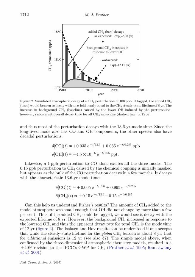
The 14 eigenvectors for the CH3Br system are shown in figure 4 and labelledwith their time constants. Most of the modes are short-lived, contain alternatesigns (zero net mass) and represent mass-conserving diffusive exchange betweenthe neighbouring points. The second longest-lived mode (1.34 yr) appears to be


4

+1yr

+2 yr+4 yr+6 yr+8 yr

0.1 1.0 10.0CH3Br mixing ratio (ppt)

0

8

12

16

20

24

28

32

36

40

44

48

52

steadystateal

titud

e (k

m)

Figure 3. Profile (solid line) of CH3Br mixing ratio (ppt) versus altitude (km) at steady statedriven by surface emissions. Also shown are the successive profiles (dashed lines) for years 1, 2, 4, 6and 8 following cut-off of CH3Br emissions. Initial loss of CH3Br occurs at a rate (1.75 yr)K1 givenby the steady-state lifetime, but slows in a few years to that of the longest-lived mode time(2.10 yr)K1 with the pattern of that mode (figure 4).

M. J. Prather1714

an exchange between the troposphere and the stratosphere. The longest-livedmode (2.10 yr) matches the pattern and time scale of the long-term decay seen infigure 3. The 10 ppt CH3Br in the zZ0 level consists of 4.8 ppt e-folding at 2.10yr, 5.0 ppt at 1.34 yr, 0.1 ppt at 0.02 yr and a small amount of the other 11modes. Thus, the decomposition into modes allows analytical prediction of long-term behaviour equivalent to the numerical integration of the continuityequation and, further, helps identify the time scales and patterns of transportbetween reservoirs.

6. Time scales for nitrous oxide: radiative coupling through ozone

Nitrous oxide (N2O), a greenhouse gas, is also a dominant source of stratosphericnitrogen oxides (NOYZNOCNO2CHNO3CN2O5C/), which catalyticallydestroy O3. The currently observed increase in N2O is consistent with anincreasing emission source from the agricultural use of nitrogen, poses a threat tothe ozone layer and contributes to global warming. Analysis of a linearized one-dimensional troposphere–stratosphere model of the N2O–NOY –O3 system interms of chemical modes (Prather 1998) shows how the radiative couplingthrough O3 shortens the time for atmospheric decay of N2O perturbations.

In the stratosphere, N2O is destroyed by direct photolysis and reaction withmeta-stable O(1D). Both reactions are controlled by O3: locally, photolysis of O3

is the source of O(1D); and globally, O3 absorbs ultraviolet sunlight, thus limitingthe photolysis rates. Stratospheric NOY is produced by the reaction of O(1D)


0.0017

048

1216202428323640444852

0.00430.0037 0.0066 0.0070 0.015 0.020

0.031

0048

1216202428323640444852

0.064 0.126 0.499 2.10 yr0.243 1.34

altit

ude

(km

)al

titud

e (k

m)

1 0 1 0 1 0 1 0 1 0 1 0 1

Figure 4. Complete set of 14 chemical modes (eigenvectors) for the one-dimensional CH3Brdiffusion model (see text) in the order of increasing mode time (yr) shown above each. Eigenvectorsare normalized to an absolute maximum of C1.


with N2O and destroyed by washout in the troposphere and photolytic loss above40 km. NOY enhances photochemical destruction of O3. Thus, even locally, theN2O–NOY –O3 system is a fully coupled chemical system, like the CH4–CO–OHsystem. A simple model includes vertical diffusion between the stratosphere andthe troposphere as for CH3Br above, assumes rapid removal of NOY and O3

below 10 km and linearizes stratospheric photochemistry in terms of the threevariables (N2O, NOY and O3) about typical atmospheric conditions. Thecontinuity equations can be solved for the steady state forced by an emissionsource of N2O in the surface level (figure 5a). The Jacobian becomes a 42!42block tridiagonal matrix with 3!3 blocks at each of the 14 vertical levels(for details, see Prather 1998). Chemical coupling is local and occurs through the3!3 blocks along the diagonal. Transport coupling is between the neighbouringlevels and is represented by the off-diagonal blocks. Since the abundance of O3 inany layer affects the absorption and scattering of ultraviolet sunlight, and hencethe photolysis rates in all layers, the radiative coupling is across all levels. Thus,the Jacobian is a sparse, but full matrix, which can nevertheless be readily solvedfor the chemical modes.


–2 +2 +6 +100

4

8

12

16

20

24

28

32

36

40

44

48

NOY

O3

10 100 1000 100001steady-state mixing ratio (ppb)

–2 +2 +6 +10

altit

ude

(km

)52

chemical modes (percentage of steady state)

chem+ trans

Tss(N2O)=127 yr T1 = 125 yr T1 = 110 yr

chem+ trans+rad N2O

(a) (b)

(i) (ii)

Figure 5. (a) Steady-state altitude profiles (parts per billion) of N2O (open circles), NOY (squares)and O3 (triangles) calculated from the one-dimensional photochemical model described in the text.Tropospheric abundances of NOY and O3 are very small and not shown. The steady-state lifetimefor N2O forced by emissions into the lowest level is 127 yr. (b) Altitude profiles of the longest-livedchemical mode of the N2O–NOy –O3 system, (i) when only local chemistry and diffusive transportare included (e-fold time T1Z125 yr) and (ii) when radiative coupling through O3 is also included(T1Z110 yr). The two modes are scaled to C10% of the steady-state abundance of N2O in thesurface level, and the profiles are plotted as percentage change relative to the steady-state profilesshown in (i).

M. J. Prather1716

Without the radiative coupling, the longest-lived mode has a mode time (T1)of 125 yr, close to the steady-state lifetime from the surface-level emissions,TSSZ127 yr. The pattern of this mode (figure 5b(i)) shows uniform perturbationsin N2O and similar perturbations in NOY with half the relative amplitude. In O3,the model produces a smaller relative depletion (opposite sign) centred about32 km, where NOY-catalysed ozone destruction has its largest impact. Thesimilarity of these two time scales almost justifies the use of TSS as the e-foldingtime for N2O emissions that is used in GWP and ODP calculations (e.g. Solomonet al. 1992). With radiative coupling (figure 5b(ii)), however, T1 drops to 110 yr,the profile of the N2O perturbation changes slightly, the NOY perturbationalmost doubles and the O3 self-healing effect gives positive perturbations in thelower stratosphere. Unlike the tropospheric CH4–CO–OH system, the N2O–NOY –O3 system has negative feedbacks: increasing N2O reduces O3 in themiddle stratosphere, allowing solar ultraviolet to destroy N2O more rapidly.

Having solved for all 42 eigenvectors, we can readily analyse perturbations.Three patterns of N2O perturbation are decomposed into the chemical modes withthe six longest time scales shown in table 1. A perturbation of 1000 kg matchingthe surface-forced steady-state profile is almost entirely mapped onto mode 1(110-yr e-fold), but 1000 kg put entirely into the surface level (effectively 0–1 km)has 1025 kg in mode 1 with the balance made up of both positive and negativeamounts in the short-lived modes. As expected, placing 1000 kg at 40 km has amuch smaller impact on the long-term burden of N2O with only 22 kg in mode 1,


Table 1. Decomposition of a perturbation into kilogram (N2O) in the first six modes of theN2O–NOY –O3 system.

perturbation

mode (yr)

110 3.1 2.0 0.68 0.66 0.60

1000 kg N2O at SSa 999.5 0 1 0 0 11000 kg N2O at 0 km 1025 2 K34 K2 1 91000 kg N2O at 40 km 22 K17 156 K74 28 252K10 DU of O3O28 km K20 0 K10 3 K5 K8

aSteady state as forced by continuous emissions at 0 km.


and most of the 1000 kg going into short-lived modes (not shown), giving a steady-state lifetime for N2O of about 3 yr! A large ozone perturbation of K10 Dobsonunits (approx. 3% of the total column), such as might result from a very large solarproton event, mostly recovers within weeks, but leaves behind a century-longdeficit of 20 kg N2O in mode 1 (as summarized in table 1).

After this analysis, several multidimensional full chemistry models (Pratheret al. 2001) examined the decay of an N2O perturbation and confirmed that theperturbation e-fold time was on average 8% less than the surface-emissionsteady-state lifetime.

7. Integrating over environmental impacts: the magic of steady state

The steady-state pattern of trace species for specified emissions can be readilycalculated using the chemical modes. Following the notation of §2, consider aperturbation, dVSS(x, y, z, n), that is the steady-state response to regular periodicemissions of trace species (n). One can treat emission sources as the addition oftrace species (n) to specific (x, y, z) locations or equivalently as a source patternS(x, y, z, n), which can be decomposed into the dimensionless eigenvectors(modes) Ei with coefficients bi , SZ

PiZ1:mbiEi. An infinitesimal amount of

emissions, S dt (kg), from time t in the past would have decayed according toeach mode time,

PiZ1:mbiEi expðKt=TiÞdt. The steady-state perturbation is, by

definition, the integral of S dt from minus infinity to the present,

dVSSh

ð0KN

Sdt ZXiZ1:m

biEi

ð0KN

expðKt=TiÞdt� �

ZXiZ1:m

TibiEi:

Assume that the source pattern S comprises only emissions of species (n), butallow for the perturbation dVSS to include all species (n

0). The mass operatorM n,defined in §2, computes the global emissions rate (kg yrK1) of species (n) in thesource pattern, Mn½S�Z

PiZ1:mbim

ni ðkg yrK1Þ, and also the global burden (kg) in

the steady-state perturbation,Mn½dVSS�ZP

iZ1:mTibimni ðkgÞ, where mn

i ZMn½Ei�is dimensionless. Thus, the steady-state lifetime of species (n) depends on thesource pattern S through the coefficients bi:

TSSðnÞhMn½dVSS�Mn½S� Z

PiZ1:m Tibim

niP

iZ1:m bimni

ðyrÞ:


M. J. Prather1718

A critical quantity in evaluating the overall environmental impact of a tracegas, such as the ODP or global warming potential, is the integrated abundance ofthe gas following a brief emission pulse. This integral needs to include not only thedecay of the primary source gas, but also the accumulation and decay of anysecondary products that impact radiative forcing or ODP. Thus, the general formwill be the integrated change in species (n0) at some location (x0, y 0, z0) followingthe initial perturbation represented by an emission pattern S(x, y, z, n) over a briefperiod D. For a short pulse of emissions, S D (kg), the atmospheric perturbationd½VDðtÞ�Z

PiZ1:mDbiEi expðKt=TiÞ can be integrated forward in time to give the

integrated impact, II (kg-yr),

II ðSDÞZðtZ0:N

dVDðtÞdt ZDXiZ1:m

TibiEiðx; y; z;n 0ÞZD dVSSðx; y; z;n 0Þ:

It can be rewritten using the definition of TSS(n) as

II ðSDÞZ dVSSðx; y; z; n 0ÞTSSðnÞMn½SD�Mn½dVSS�

� �:

Thus, the overall integrated perturbation caused by emission of a trace gas,including all secondary impacts, is given exactly by the steady-state pattern in allspecies multiplied by the steady-state lifetime of species (n) and then scaled by theratio of the amount of n in the pulse to that in the steady-state pattern.

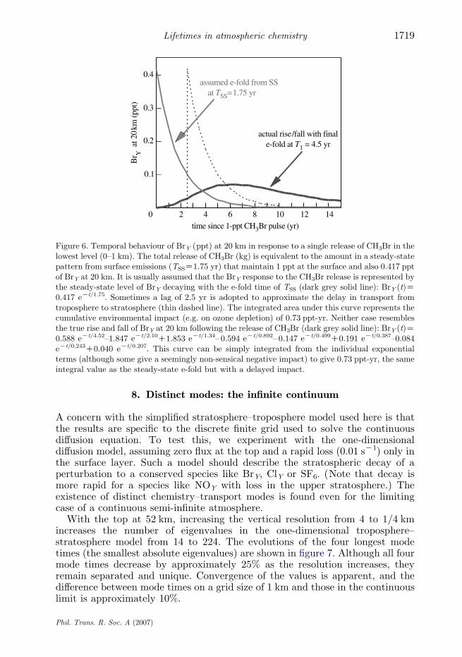
As an example, consider the ODP in response to the release of CH3Br at thesurface. The ozone depletion can be approximated by the perturbation to BrY at20 km as shown in figure 6. There is a delay in the impact, as CH3Br istransported into the stratosphere and is chemically converted into BrY (darkgrey solid line). A peak in BrY is reached ca 6 yr following the release and isfollowed by a slow decay with the mode time of 4.52 yr, corresponding to theremoval of a conservative tracer from the stratosphere. In this case, the release(kg) is scaled to be the amount of CH3Br present in the atmosphere for a steady-state distribution forced by surface emissions resulting in 1 ppt at the surface.The area under the BrY curve is 0.73 ppt-yr. As shown above, this integral isexactly equal to the product of the steady-state lifetime for CH3Br with surfaceemissions (1.75 yr) and the steady-state abundance of BrY at 20 km (0.42 ppt). Itis almost universally assumed in assessments of ODP or climate forcing (Solomonet al. 1992; WMO 1995; IPCC 1996) that this integral is represented by a singlee-fold decay of 1.75 yr (light grey solid line). Fortunately, the integrated impactis correctly evaluated with this assumption, but the time scale is not. Even with a2.5-yr delay to allow for CH3Br to reach the stratosphere (dashed line), the timescale of the response is incorrect (see Ko et al. 1997 for discussion). This mistakenview of time scales has led to the false reasoning in Montreal Protocolnegotiations that reductions in CH3Br would provide recovery of ozone within afew years: they do not.

The theory developed here applies readily to very short lived species, such as1-C3H7Br, with a tropospheric residence time of weeks (Bridgeman et al. 2000;Olsen et al. 2000, Wuebbles et al. 2001). It provides a formal basis for computingthe environmental impact using the readily calculated annual steady-statepattern of impacts (e.g. BrY) scaled by the annual steady-state lifetime of thesource gas.


0 2 4 6 8 10 12 14time since 1-ppt CH3Br pulse (yr)

0.1

0.2

0.3

0.4

Br Y

at 2

0km

(ppt

)

assumed e-fold from SS at TSS=1.75 yr

actual rise/fall with finale-fold at T1 = 4.5 yr

Figure 6. Temporal behaviour of BrY (ppt) at 20 km in response to a single release of CH3Br in thelowest level (0–1 km). The total release of CH3Br (kg) is equivalent to the amount in a steady-statepattern from surface emissions (TSSZ1.75 yr) that maintain 1 ppt at the surface and also 0.417 pptof BrY at 20 km. It is usually assumed that the BrY response to the CH3Br release is represented bythe steady-state level of BrY decaying with the e-fold time of TSS (dark grey solid line): BrY (t)Z0.417 eKt/1.75. Sometimes a lag of 2.5 yr is adopted to approximate the delay in transport fromtroposphere to stratosphere (thin dashed line). The integrated area under this curve represents thecumulative environmental impact (e.g. on ozone depletion) of 0.73 ppt-yr. Neither case resemblesthe true rise and fall of BrY at 20 km following the release of CH3Br (dark grey solid line): BrY (t)Z0.588 eKt/4.52–1.847 eKt/2.10C1.853 eKt/1.34– 0.594 eKt/0.892– 0.147 eKt/0.499C0.191 eKt/0.387–0.084eKt/0.243C0.040 eKt/0.207. This curve can be simply integrated from the individual exponentialterms (although some give a seemingly non-sensical negative impact) to give 0.73 ppt-yr, the sameintegral value as the steady-state e-fold but with a delayed impact.


8. Distinct modes: the infinite continuum

A concern with the simplified stratosphere–troposphere model used here is thatthe results are specific to the discrete finite grid used to solve the continuousdiffusion equation. To test this, we experiment with the one-dimensionaldiffusion model, assuming zero flux at the top and a rapid loss (0.01 sK1) only inthe surface layer. Such a model should describe the stratospheric decay of aperturbation to a conserved species like BrY, ClY or SF6. (Note that decay ismore rapid for a species like NOY with loss in the upper stratosphere.) Theexistence of distinct chemistry–transport modes is found even for the limitingcase of a continuous semi-infinite atmosphere.

With the top at 52 km, increasing the vertical resolution from 4 to 1/4 kmincreases the number of eigenvalues in the one-dimensional troposphere–stratosphere model from 14 to 224. The evolutions of the four longest modetimes (the smallest absolute eigenvalues) are shown in figure 7. Although all fourmode times decrease by approximately 25% as the resolution increases, theyremain separated and unique. Convergence of the values is apparent, and thedifference between mode times on a grid size of 1 km and those in the continuouslimit is approximately 10%.


0.1

1.0

10.0

mod

e tim

e sc

ale

(yr)

grid size (km)0.1 1.0 10.04.00.25

Figure 7. Convergence of the four longest mode times in a one-dimensional diffusion model as thegrid size decreases from 4 to 0.25 km. The model has typical troposphere–stratosphere diffusioncoefficients (see text) with zero flux at the top (zZ52 km) and rapid loss (0.01 sK1) only in thesurface layer (zZ0 km).

M. J. Prather1720

Providing a solution for the modes on a semi-infinite atmosphere poses adifferent problem. With an infinite upper boundary and constant diffusioncoefficient K, Waugh & Hall (2002, reaction 9) show that the Green’s functionused for age of air has an analytical form that precludes the simple exponentialdecay of the eigenvalue decomposition. In the stratosphere, typical profiles for Khave it increasing as density N decreases (Ehhalt et al. 2004), and thus far wehave chosen K/NK1. In this test, three cases are chosen near the Waugh andHall limiting form: (i) K/NK0.05, (ii) K/NK0.01, and (iii) K/constant.Leaving the grid step at 4 km, the one-dimensional model top is increased from68 to 828 km (18 to 208 modes), and the evolution of the four longest mode timesfor each case is shown in figure 8. For case (i), the four solid lines show increasingmode times until the top reaches 200 km, with no change thereafter. For moreslowly increasing K, case (ii), the four dashed lines show similar behaviouralthough the second through fourth longest mode times are still shifting evenwhen the top reaches 828 km. For the previous examples with K/NK1, the fourlongest mode times have converged to within 1% when the model top reaches68 km. For case (iii), however, raising the upper boundary indeed changes thecharacter of the chemistry–transport modes (dotted lines), and we approach acontinuum of long-lived modes as anticipated.

9. The stratospheric decay mode: observed age of air,tritium and chlorine

The age of air in the stratosphere is defined as the time since the air was last inthe troposphere, and the mean age can be directly observed with quasi-conservedtrace gases that are increasing at a regular rate (e.g. CO2, SF6). In models, the


0

5

10

15

20

25

four

long

est m

ode

times

(yr

)K = constant

0

5

10

15

K = A N–0.01

0

5

10

15

200 400 600 800

top of model (km)

K = A N–0.05

Figure 8. Convergence of the four longest mode times in a one-dimensional diffusion model(figure 7) as the top of the model increases from 68 to 828 km. Results are shown for differentdependences of the diffusion coefficients K on the density N: KZconstant A (four dotted lines),KZANK0.01 (dashed lines) and KZANK0.05 (solid lines). An infinite atmosphere with constant Khas no modes (dotted), but if K has only a slight inverse dependence on N, then the long-livedmodes appear as distinct even as the upper boundary approaches infinity.


age of air can be calculated as a spectrum of ages from which the mean age can beevaluated (Waugh & Hall 2002). The mean age is related to the chemical modes.Specifically, the tail end of the spectrum corresponds to the mode describingstratospheric decay of a conserved tracer (see discussion above and Hall et al.1999). The observed decay of stratospheric tritium (3H) injected by atmosphericnuclear tests in the 1960s looks like a chemical mode (Ehhalt et al. 2004). The lagin recovery of upper stratospheric HCl following the decline of tropospheric


M. J. Prather1722

chlorofluorocarbons and other halocarbons in the 1990s is also a measure of theage of air spectrum and the long-lived modes (see discussion in Waugh & Hall2002). Together, these observations provide the only current observational testof chemical modes.

A clear demonstration of the stratospheric decay mode was found with theModels and Measurements II project (Hall et al. 1999). For each model used tocompute the age-of-air spectra, the original request had been to integrate10–20 yr to ensure that the tail of the spectrum was well defined. Recognitionthat this tail represented the decay mode and that for each model it followed thesame exact e-fold time throughout the stratosphere, however, enabledsubstantial savings in computation and a far easier evaluation of the mean ageonly after 6–10 yr of integration. In addition, Hall et al. (1999) and Ehhalt et al.(2004) showed that for all but one of the three-dimensional models, there was asimple linear relationship between the mean age at 30 km and the decay mode’se-fold time.

Several years after injection, the decay of stratospheric tritium (as waterabove 20 km) followed a single exponential decay from 1969 to 1984. Whencorrected for the radioactive decay of tritium, this gives a decay mode time of7.7G2 yr (Ehhalt et al. 2004). Allowing for a trend in stratospheric water that isconsistent with the limited measurements, this decay mode time drops to 6.9years. Corresponding mode times derived from the observed mean age rangefrom 3.8 to 5.3 yr. Given the uncertainties associated with both of thesederivations, a mode time between 5 and 6 yr is probable. Unfortunately, thesevalues are still outside the range of decay mode times for all but one of the three-dimensional models, i.e. 1.44–4.75 yr (see table 2 of Ehhalt et al. 2004).

10. Chemistry–transportmodes: three-dimensional tropospheric chemistry

In realistic simulations of global atmospheric chemistry with a three-dimensionalchemistry–transport model (CTM), the continuity equation operators (Chem,Trans and Rad) change every hour or so. Presuming that this change is cyclic(e.g. the 24 h cycle of photolysis rates, the seasonal cycles of meteorologicaltransport), the chemical modes should still exist but include another dimensionthat describes the temporal behaviour of perturbations over the daily/yearlycycle; e.g. Ei(x, y, z, n, t). Indeed, the existence of the long-lived, seasonallyvarying, CH4-like, tropospheric chemistry mode has been sought for andcharacterized in at least two CTMs (Wild & Prather 2000; Derwent et al.2001). The stratospheric decay mode was identified after the fact in many CTMsthrough the age-of-air experiments (Hall et al. 1999).

The number of CTM modes with an annually repeating meteorology readilyexceeds 108, precluding the complete chemical mode decomposition shown in§§3–8. The longest-lived mode, however, can still be characterized by followingthe decay of perturbations. Wild & Prather (2000) and Derwent et al. (2001)found the decadal tropospheric mode (CH4–CO–OH–NOx–/) of their CTMs bytracking a perturbation run minus control run for a decade following severaldifferent perturbations to tropospheric chemistry. (These CTMs did not includefeedbacks with stratospheric chemistry that would have excited the century-longstratospheric N2O-like mode.)


year of CTM run

–5–4–3–2–100

0.05

0.10

0.15

0.20

00.20.40.60.81.0

0

20

40

60

perturbperiod

ppt

ppb

ppb

ppb

pert

urba

tion

min

us c

ontr

ol

(a)

(b)

(c)

(d )

109876543210

Figure 9. Perturbations to (a) CH4 (ppb), (b) CO (ppb), (c) O3 (ppb) and (d ) NOx (ppt) at MaceHead, Ireland (538 N, 108W) caused by a 1-yr, 20% increase in global CH4 emissions. The decay ofthis perturbation is followed for 9 yr after return of CH4 emissions to normal levels. Results areshown for the perturbation minus control runs with a three-dimensional global chemistry–transport model.


In one numerical experiment, Wild et al. increased global CH4 emissions by20%. The resulting perturbations to the CH4, CO, O3 and NOx abundancessimulated for Mace Head, Ireland are shown in figure 9. During the perturbationyear, abundances of CH4, CO and O3 rise, while that of NOx falls. After theperturbation to emissions ceases (year 1), there are rapid decays involving short-lived modes, but within a few years, the perturbation curves assume the regularpattern of a repeating annual cycle that decays over any 12-month period withan e-fold time of 14.2 yr. Wild et al. extracted the longest-lived mode from theseexperiments, and the zonal-mean, mid-tropospheric, latitude-by-season patternsof CH4 and CO are shown in figure 10. The modes are dimensionless and arescaled to an absolute abundance of a single species as one point in space andtime. In this example, the mode has been scaled to have an annual mean CH4

perturbation of 100 ppb. The e-fold has been removed to show the annuallyrepeating patterns. The seasonal variation in the CH4 perturbation, 98–102 ppb,is similar to that in CO, 1–3 ppb, but with opposite phase in both latitude andseason. The large annual variations of the mode at mid-latitudes indicate theimportance of seasonal photochemistry.


Jan Jul Jan Jul Jan Jul

98100

102

month

(a)

1

2

3(b)

– 90– 60

– 30

0

3060

latit

ude

Jan Jul Jan Jul Jan Jul

month

Figure 10. Zonal-mean, mid-tropospheric, seasonal patterns of (a) CH4 (ppb) and (b) CO (ppb) inthe primary, 14.2-yr mode of a three-dimensional global tropospheric chemistry–transport modelwith annually repeating meteorology. The e-fold of the perturbation has been removed to show theannually repeating patterns. The mode has been scaled to have an annual mean CH4 perturbation of100 ppb. Similar patterns (not shown) exist for O3, NOx and most other chemically reactive species.

M. J. Prather1724

Tropospheric chemistry in these CTMs has only one dominant long-livedmode. Once it has been characterized for a given atmospheric simulation, itsproperties can be used to extrapolate almost all perturbations based on thatcontrol simulation. (Long-lived gases such as CHF2Cl that are present in verylow abundances will also produce decadal modes, but with very smallamplitudes.) Recognizing this, both Derwent et al. (2001) and Wild et al.(2001) studied a wide range of perturbations to short-lived species such as NOx

and CO. They calculated the long-term climate impacts from 4-yr CTMsimulations by integrating the short-term changes in O3 and then deriving theamplitude of the long-lived mode to explicitly integrate over the decadal changesin CH4 and O3.

11. Development and future directions

The chemical coupling between the stratosphere and the troposphere remainslargely unexplored. Thus far, we have separately identified the CH4-liketropospheric and N2O-like stratospheric chemical modes. However, the CH4-likemode will perturb stratospheric O3 directly through reactions involving CH4 andindirectly by increasing stratospheric H2O. Changes in stratospheric O3 willperturb N2O and also tropospheric CH4 chemistry through changing photolysisrates and OH. Lower-dimension models (e.g. §§3–9) may not accurately representthe stratosphere–troposphere coupling, but CTM studies of any chemicalperturbation with an N2O-like mode will need to integrate the perturbation-minus-control simulations for 50 yr or more to separate these two modes.

A practical breakthrough could be achieved if global atmospheric chemistrycan be approximated by a finite Jacobian. For a reasonable number of degrees offreedom (e.g. 1000), the system can be solved for all eigenvectors. If such amatrix represented most of the important chemical modes, then it wouldprovide an explicit model for following the response to perturbations to any



atmospheric species at any location. The challenge here is defining the space–time averaging kernels to reduce the dimensionality of the system whilepreserving the major modes.

One practical concern is whether the long-lived modes remain identifiable overthe year-to-year variations in meteorology. Although different CTMs withdifferent meteorological fields produce similar modes for stratospheric decay ortropospheric CH4 chemistry, they are different enough to preclude readyevaluation of long-term impacts. Work with a single CTM and successiveyears of forecast meteorological fields is ongoing and should provide aquantitative measure of how the excitation and decay of chemical modes dependon meteorology. Similar questions arise regarding large year-to-year variations inatmospheric composition, such as for years with extensive forest fires.

Moving beyond atmospheric chemistry, extension of this approach to Earthsystem models could yield surprises. The coupling across different components ofthe chemistry–climate system, such as atmospheric chemistry, carbon cycle,marine biogeochemistry, aerosols and climate, may introduce new linkages andalter our expectation of the time scales of anthropogenic climate perturbations.Defining and computing these coupled chemistry–climate modes will be challenging.

This researchwas supported by theNational Science Foundation (ATMATM-0550234), theNational

Aeronautics and Space Administration (NNG06GB84G, NNG04GF90G and NNG04GA09G) and

the Kavli Foundation. I thank J. Neu for careful review and suggestions on the manuscript.

References

Bolin, B. & Rodhe, H. 1973 Note on concepts of age distribution and transit-time in natural

reservoirs. Tellus 25, 58–62.

Bridgeman, C. H., Pyle, J. A. & Shallcross, D. E. 2000 A three-dimensional model calculation of

the ozone depletion potential of 1-bromopropane (1-C3H7Br). J. Geophys. Res. 105,

26 493–26 502. (doi:10.1029/2000JD900293)

Butler, J. H. 1994 The potential role of the ocean in regulating atmospheric CH3Br. Geophys. Res.

Lett. 21, 185–188. (doi:10.1029/94GL00071)

Chapman, S. 1930 A theory of upper-atmosphere ozone. Mem. R. Meteorol. Soc. 3, 103–125.

Church, J. A., White, N. J. & Arblaster, J. M. 2005 Significant decadal-scale impact of volcanic

eruptions on sea level and ocean heat content. Nature 438, 74–77. (doi:10.1038/nature04237)

Derwent, R. G., Collins, W. J., Johnson, C. E. & Stevenson, D. S. 2001 Transient behaviour of

tropospheric ozone precursors in a global 3-D CTM and their indirect greenhouse effects. Clim.

Change 49, 463–487. (doi:10.1023/A:1010648913655)

Ehhalt, D. H., Rohrer, F., Schauffler, S. & Prather, M. 2004 On the decay of stratospheric

pollutants: diagnosing the longest-lived eigenmode. J. Geophys. Res. 109, D08 102. (doi:10.

1029/2003JD004029)

Farrell, B. F. & Ioannou, P. J. 2000 Perturbation dynamics in atmospheric chemistry. J. Geophys.

Res. 105, 9303–9320. (doi:10.1029/1999JD901021)

Fisher, D. A. 1995 Calculated lifetimes and their uncertainties. In Proc. Workshop on Atmospheric

Degradation of HCFCs and HFCs, Boulder, CO, 17–19 November 1993, pp. 1–5. Washington,

DC: AFEAS Program Office section 3.

Hall, T. H. et al. 1999 Transport experiments. In Models and measurements intercomparison II,

Rep. NASA/TM-1999-20,9554 (eds J. H. Park et al.), ch. 2, pp. 110–189. Hampton, VA: NASA.

IPCC 1996 Climate change1995. InThe science of climate change, IntergovernmentalPanel onClimate

Change (eds J. T. Houghton et al.), p. 572. Cambridge, UK: Cambridge University Press.


http://dx.doi.org/doi:10.1029/2000JD900293

http://dx.doi.org/doi:10.1029/94GL00071

http://dx.doi.org/doi:10.1038/nature04237

http://dx.doi.org/doi:10.1023/A:1010648913655




M. J. Prather1726

Isaksen, I. S. A. & Hov, O. 1987 Calculation of trends in tropospheric O3, OH, CH4, and NOx.Tellus B 39, 271–285.

Junge, C. E. 1974 Residence time and variability of tropospheric trace gases. Tellus 26, 477.Ko, M. K. W., Sze, N. D., Scott, C. J. & Weisenstein, D. K. 1997 On the relation between

stratospheric chlorine/bromine loading and short-lived tropospheric source gases. J. Geophys.Res. 102, 25 507–25 517. (doi:10.1029/97JD02431)

Manning, M. R. 1999 Characteristic modes of isotopic variations in atmospheric chemistry.Geophys. Res. Lett. 26, 1263–1266. (doi:10.1029/1999GL900217)

Olsen, S. C., Hannegan, B. J., Zhu, X. & Prather, M. J. 2000 Evaluating ozone depletion from veryshort-lived halocarbons. Geophys. Res. Lett. 27, 1475–1478. (doi:10.1029/1999GL011040)

O’Neill, B. C., Gaffin, S. R., Tubiello, F. N. & Oppenheimer, M. 1994 Reservoir timescales foranthropogenic CO2 in the atmosphere. Tellus-B 46, 378–389. (doi:10.1034/j.1600-0889.1994.t01-4-00004.x)

Prather, M. J. 1994 Lifetimes and eigenstates in atmospheric chemistry. Geophys. Res. Lett. 21,801–804. (doi:10.1029/94GL00840)

Prather, M. J. 1996 Time scales in atmospheric chemistry: theory, GWPs for CH4 and CO, andrunaway growth, Geophys. Res. Lett. 23, 2597–2600. (doi:10.1029/96GL02371)

Prather, M. J. 1997 Timescales in atmospheric chemistry: CH3Br, the ocean, and ozone depletionpotentials. Global Biogeochem. Cycles 11, 393–400. (doi:10.1029/97GB01055)

Prather, M. J. 1998 Time scales in atmospheric chemistry: coupled perturbations to N2O, NOy,and O3. Science 279, 1339–1341. (doi:10.1126/science.279.5355.1339)

Prather, M. J. 2002 Lifetimes of atmospheric species: integrating environmental impacts. Geophys.Res. Lett. 29, 2063. (doi:10.1029/2002GL016299)

Prather, M., Derwent, R., Ehhalt, D., Fraser, P., Sanhueza, E. & Zhou, X. 1995 Other tracer gasesand atmospheric chemistry In Climate change 1994, Intergovernmental Panel on ClimateChange (eds J. T. Houghton et al.), ch. 2, pp. 73–126. Cambridge, UK: Cambridge UniversityPress.

Prather, M. et al. 2001 Atmospheric chemistry and greenhouse gases (eds J. T. Houghton et al.),ch. 4, pp. 239–287. Cambridge, UK: Cambridge University Press.

Ramaswamy, V., Boucher, O., Haigh, J., Hauglustaine, D., Haywood, J., Myhre, G., Nakajima, T.,Shi, G. Y. & Solomon, S. 2001 Radiative forcing of climate change. In Climate change 2001: thescientific basis (eds J. T. Houghton et al.), ch. 6, pp. 349–416. Cambridge, UK: CambridgeUniversity Press.

Solomon, S., Mills, M., Heidt, L. E., Pollock, W. H. & Tuck, A. F. 1992 On the evaluation of ozonedepletion potentials. J. Geophys. Res. 97, 825–842.

Waugh, D. W. & Hall, T. M. 2002 Age of stratospheric air: theory, observations, and models. Rev.Geophys. 40, 1010. (doi:10.1029/2000RG000101)

Wild, O. & Prather, M. J. 2000 Excitation of the primary tropospheric chemical mode in a globalthree-dimensional model. J. Geophys. Res. 105, 24 647–24 660. (doi:10.1029/2000JD900399)

Wild, O., Prather, M. J. & Akimoto, H. 2001 Indirect long-term global cooling from NOxemissions. Geophys. Res. Lett. 28, 1719–1722. (doi:10.1029/2000GL012573)

WMO 1995 Scientific assessment of ozone depletion: 1994, global ozone research and monitoringproject. Report no. 37, World Meteorological Organization, Geneva.

Wuebbles, D. J., Patten, K. O., Johnson, M. T. & Kotamarthi, R. 2001 New methodology forozone depletion potentials of short-lived compounds: n-propyl bromide as an example.J. Geophys. Res. 106, 14 551–14 571. (doi:10.1029/2001JD900008)





http://dx.doi.org/doi:10.1034/j.1600-0889.1994.t01-4-00004.x

http://dx.doi.org/doi:10.1034/j.1600-0889.1994.t01-4-00004.x



http://dx.doi.org/doi:10.1029/97GB01055

http://dx.doi.org/doi:10.1126/science.279.5355.1339


http://dx.doi.org/doi:10.1029/2000RG000101




Lifetimes and time scales in atmospheric chemistry

Documents

Transcript of Lifetimes and time scales in atmospheric chemistry