IEICE TRANS. COMMUN., VOL.E95–B, NO.5 MAY 20121651

PAPER

Lifetime-Aware Battery Allocation for Wireless Sensor Networkunder Cost Constraints∗

Yongpan LIU†a), Member, Yiqun WANG†, Hengyu LONG†, and Huazhong YANG†, Nonmembers

SUMMARY Battery-powered wireless sensor networks are prone topremature failures because some nodes deplete their batteries more rapidlythan others due to workload variations, the many-to-one traffic pattern, andheterogeneous hardware. Most previous sensor network lifetime enhance-ment techniques focused on balancing the power distribution, assuming theusage of the identical battery. This paper proposes a novel fine-grainedcost-constrained lifetime-aware battery allocation solution for sensor net-works with arbitrary topologies and heterogeneous power distributions.Based on an energy–cost battery pack model and optimal node partition-ing algorithm, a rapid battery pack selection heuristic is developed and itsdeviation from optimality is quantified. Furthermore, we investigate theimpacts of the power variations on the lifetime extension by battery alloca-tion. We prove a theorem to show that power variations of nodes are morelikely to reduce the lifetime than to increase it. Experimental results indi-cate that the proposed technique achieves network lifetime improvementsranging from 4–13× over the uniform battery allocation, with no more than10 battery pack levels and 2-5 orders of magnitudes speedup compared witha standard integer nonlinear program solver (INLP).key words: wireless sensor network, battery allocation, lifetime-aware

1. Introduction

Wireless Sensor Networks (WSN) are distributed data ac-quisition systems consisting of numerous wireless sensornodes. They have the potential to allow sensing in appli-cations and environments where it was previously impossi-ble or prohibitively expensive. For example, WSNs may beused in weather monitoring, security, tactical surveillance,disaster management, and intelligent traffic control applica-tions [2]. Infrastructure-free operation is one of their pri-mary advantages. However, this beneficial attribute intro-duces a penalty. Distributed infrastructure-free operationsin the remote locations make replacing batteries expensive.Energy constraints are therefore extremely tight.

Due to the limited energy capacity enforced by the lowcost requirement of WSNs, the lifetime of a WSN to executecontinuous monitoring tasks is critical. It is desirable that allnodes in WSN should cooperate with each other to sense andtransmit information and run out of energy together. Other-wise, nodes in some areas will be unable to transmit theirsensing data to the collective node because other battery de-pleted nodes will break the transmission routes to those ar-eas. However, the many-to-one traffic pattern in WSN nat-urally leads to an imbalance power distribution. Previous

Manuscript received October 19, 2010.Manuscript revised October 25, 2011.†The authors are with the Electronic Engineering Department,

Tsinghua University,100084, Beijing, P.R. China.∗This paper was presented at ICCAD2009 [1].

a) E-mail: ypliu@tsinghua.edu.cnDOI: 10.1587/transcom.E95.B.1651

work had shown that such an imbalance will serious shortenthe lifetime of a WSN.

Recently, research work attempted to balance theenergy consumption of the network by constructing thelifetime-aware WSN with heterogeneous nodes, since mov-ing tasks among the nodes to balance power is not en-ergy efficient. By providing the nodes in the second tierstronger processing ability and larger battery capacity, Houet al. [3] presented a two-tier lifetime-aware infrastructure.Wu et al. [4] presented a non-uniform node deployment toexploit more relay nodes to deal with the power peak in thetraffic-heavy area to prolong the lifetime. Several other re-searchers [5], [6] illustrated a mobile sink or multiple sinksapproach to adjust the traffic flow and thus the energy dis-tribution. Others proposed a battery allocation technique[1], [7] to equip power-hungry sensor nodes with differentbattery packs to relieve the imbalance. Among the abovelifetime-aware techniques, the heterogeneous battery alloca-tion received more and more attentions due to its less over-heads on the original WSN.

Sichitiu et al. [7] were the first to report that equippingsensor nodes with different battery capacities can prolongthe WSN lifespan. However, their formulation has two ma-jor drawbacks: First, their battery allocation object is thecoarse-grained network tier instead of the fine-grained node,i.e. the sensor nodes in each tier are equipped with the samebattery and it can not deal with the power imbalance withineach network tier; Second, they assumed a monolithic powerdistribution in a circular WSN from the leaf nodes to the sinknode, i.e. it is inapplicable to the WSNs with multiple dis-tributed power peaks, which is common in the WSNs thatadopt clustering or multiple sinks or other energy efficientrouting techniques; Those limitations prevent the method tobe used in the real WSNs. Instead of those drawbacks, thispaper proposed a novel fine-grained node-level battery al-location for the battery-powered networked embedded sys-tems. Our work makes the following contributions:

1. We presented a novel fine-grained node-level batteryallocation method under cost constraints. It is formu-lated as an integer nonlinear programming problem anda quite efficient heuristic is built based on the provedoptimal node partitioning theorem and the energy-costmodel for the battery packs.

2. We discussed the impacts of power variations on thelifetime extensions using the battery allocation method.Theoretical analysis shows that the power variations

Copyright© 2012 The Institute of Electronics, Information and Communication Engineers

1652IEICE TRANS. COMMUN., VOL.E95–B, NO.5 MAY 2012

of the nodes are more likely to reduce the lifetime ofWSNs than to increase it. It implies that a larger packlevel over a threshold is no need considering the powervariations.

3. Experiments indicate that the proposed method canprolong the lifetime by 4–13× with no more than 10battery pack levels compared with the uniform bat-tery allocation approach. Furthermore, the heuristicachieves 2–5 orders of magnitudes speedup and longertime improvements compared with a standard integernonlinear program (INLP) solver.

After we discuss the motivation of this work in the followingSect. 2, the node-level battery allocation problem is formu-lated in Sect. 3. The battery allocation problem is solved inSect. 4 and the power variations’ impacts on it are analyzedin Sect. 5. Section 6 presents the experimental results. Weconclude the challenges and future work in Sect. 7.

2. Motivation

This section describes the motivation of the lifetime-awarebattery allocation method for WSNs with various topolo-gies, node configurations, and power distributions.

First of all, we define the lifetime-aware design flowfor WSNs. Figure 1 shows the lifetime-aware flow to ex-tend the working time of WSN to meet the requirements.As we can see, the major difference between the traditionalperformance-driven flow and the lifetime-aware one, is thedesign objective changing to the lifetime under certain con-straints, such as costs and performance. The power analy-sis stage will estimate the power consumption of each nodebased on the initial WSN deployment and network proto-cols. In the second stage, the power balancing techniquesare adopted to relieve the power imbalance and extend thelifetime. However, the power imbalance is very difficult tobe eliminated due to the essential many-to-one communi-cation pattern in WSNs. Therefore, the battery allocationmethod is used in the third stage.

Figure 2 shows a typical power distribution of a WSNusing power-balanced compression and clustering tech-niques [8]. Obviously, the difference between sensor nodesare significant. Assuming that the total energy is denotedas Etot and a uniform battery allocation is used, each sensornode is equipped with a battery containing Etot/n energy.The first sensor node failure time Tlife can be decided byTlife = Etot/(n · pmax), where pmax is the maximum powerconsumption in all sensor nodes. The doted line indicatesthe power level at which the maximum-power (pmax) sensornode depletes its battery. The batteries of the sensor nodeslocated in the diagonal line region still have energy but theycannot be used due to the failure of other nodes. Therefore,a heterogeneous battery allocation in Fig. 1 will help to ex-tend the lifetime.

The above example motivates the primary researchquestions addressed in this paper: Given a budget of en-ergy cost for a WSN with arbitrary topology, node configu-

Fig. 1 Lifetime-aware deploying flow of WSN.

Fig. 2 Uniform vs. 2-level battery allocation.

ration, and power distribution, how should battery energy beassigned to sensor nodes to maximize the network lifetimeunder constraints on cost and the number of available batterypack levels? The solution should include the lifetime-awarenode partitioning to enable battery pack capacities and bat-tery allocations to be determined. Furthermore, to make thebattery allocation technique more practical, we need alsoevaluate the impact of the power variations on the techniqueto prolong the lifetime of the WSNs.

3. Problem Formulation

This section first formulates a battery pack assignment prob-lem and then analyzes the complexity of the searching spaceto show the necessity to develop a heuristic algorithm in thenext section.

3.1 Problem Formulation

Before illustrating the lifetime-aware battery allocation al-gorithm, we first define the following terms. Let P =

(p1, p2, . . . , pn) be the power distribution of the n−node net-work. There are m types of batteries with energy capacitiesE1, E2, . . . , Em and costs C1,C2, . . . ,Cm. The relationshipbetween energy and cost is represented as follows: Ci =

f (Ei), i = 1, . . . ,m. By combining battery units into packs,

LIU et al.: LIFETIME-AWARE BATTERY ALLOCATION FOR WIRELESS SENSOR NETWORK UNDER COST CONSTRAINTS1653

M types of battery pack levels Epk{1}, Epk{2}, . . . , Epk{M} areachieved. If ω(i, k) denotes the number of battery units kassigned to battery pack i, then Epk{i} =

∑mk=1 ω(i, k) · Ek.

Each node is equipped with one battery pack. The sensornodes are divided into M sets: L1, L2, . . . , LM. Each Li hasNi nodes, and each node in Li is assigned a battery packEpk{i}, i = 1, 2, . . . ,M.

By defining the network lifetime as the first node fail-ure time, the working time of node set Li is

Ti =Epk{i}gi=

∑mk=1 ω(i, k) · Ek

gi, i = 1, . . . ,M (1)

where gi is the maximum power in Li. The lifetime of thesystem is therefore

T =M

mini=1

Ti (2)

The battery allocation problem is formulated as fol-lows: given a cost constraint Ctotal ≤ Ccons and the num-ber of battery pack M, determine the number of the batteryunits in the each level to maximize T . The total cost can berepresented as

Ctotal =

M∑i=1

⎛⎜⎜⎜⎜⎜⎝Ni ·m∑

k=1

ω(i, k) · f (Ek)

⎞⎟⎟⎟⎟⎟⎠ (3)

The optimization objective is now formulated as fol-lows:

T =M

mini=1

(∑mk=1 ω(i, k) · Ek

gi

)→ max (4)

subject to:

1.∑M

i=1

(Ni ·∑m

k=1 ω(i, k) · f (Ek))≤ Ccons

2. ω(i, k) is a nonnegative integer, i = 1, . . . ,M and k =1, . . . ,m

3.2 Complexity Analysis

Given a capacity-price function Ci = f (Ei), i = 1, . . . ,m, theoptimization problem is formulated as an INLP that can besolved by a standard INLP solver, such as LINGO. However,experimental results will demonstrate that the running timeof a general INLP solver is too long to be tolerated. Thecomplexity of such a problem is illustrated as below. Be-cause any node can be equipped with several batteries withdifferent capacities, the search space is extremely large. As-suming the case with n nodes and m battery types, the timecomplexity is O((Dim + 1)m×n), where Dim is a constantspecifying the maximum number of each battery assigned toeach pack. When m = 5, M = 10 and n = 100, the computa-tion complexity reach 102300. Though, smart algorithms canbe adopted in the commercial solvers to reduce such a hugesearch space, our experimental results in Sect. 6 showed thatit failed to solve the problem in 24 hours when the networksize is larger than 64. Therefore, a faster heuristic algorithm

is necessary.

4. Battery Allocation Algorithm

Figure 3 shows the flowchart of the proposed method. Thefirst step is shown in the dotted block, in which the sensornodes are partitioned into M sets to allow the lifetime ofwireless sensor network to be optimized in the second step.Based on the partitioning, the second step in the upper-leftblock presents a CLPS (Cost Limited Pack Select) heuris-tic algorithm to choose proper battery pack configurationsfor each set. Finally, the node set partition, the correspond-ing battery pack configuration, and the lifetime of wirelesssensor network are produced.

4.1 Optimal Partition to Maximize the Lifetime

This section describes a technique to divide the sensor nodesinto M sets. As the later section has pointed out, the costconstraint Ccons could be transformed as the total energyconstraint Econs, we do the node partition based on the en-ergy constraint. The relationship between Ccons and Econs

will be stated in Sect. 4.2.1. Given the power distribution ofsensor nodes in a WSN and the set number, we need the sen-sor node partition achieving the maximum network lifetime.First, we present a theorem on the lifetime as below:

Theorem 1: Given an energy constraint Econs and thepower distribution p1, p2, . . . , pn, the network lifetime un-der any node partition of M sets will at most be

T =Econs∑M

i=1(gi · Ni)(5)

where gi is the maximum power consumption in set Li, andNi is the number of nodes in Li.

Theorem 1 is proven in Appendix A. It shows the max-imum lifetime of a given node partition. The lifetime is re-lated to gi and Ni and varies under different node partitions.

Next, we will show how to achieve the optimal partitionto maximize T . Based on Eq. (5), achieving the maximum Tis simplified as the minimum value problem of

∑Mk=1(gk ·Nk)

Fig. 3 Proposed method flow: Optimal partition and CLPS algorithm.

1654IEICE TRANS. COMMUN., VOL.E95–B, NO.5 MAY 2012

when Econs is fixed.To divide the nodes into M sets, we first sort the power

consumption of nodes p1, p2, . . . , pn in an ascending orderas q1 ≤ q2 ≤ . . . ≤ qn. We define M + 1 boundary points toindicate the partition, where xi and xi−1 denote the index oftwo boundary nodes in set Li−1. Thus, the number of nodesin set Li−1 is Ni−1 = xi − xi−1. As xi is the largest index inset Li−1, gi−1 = qxi . Therefore, the optimization problem isrepresented as:

Vdisc =

M∑k=1

(gk ·Nk) =M+1∑i=2

(qxi × (xi− xi−1)) → min (6)

where xi is the optimizing variables, i = 1, 2, . . . ,M + 1.They stand for the node number in the sorted power distri-bution q1, q2, . . . , qn. The constraint conditions are listed asthe following:

1. xi is a nonnegative integer, i = 1, . . . ,M + 1.2. x1 = 0, xM+1 = n.3. xi > xi−1, i = 2, . . . ,M + 1.

This problem differs from the traditional nonlinear pro-gramming formulation because the variables are the sub-scripts of a discrete mapping. As the objective func-tion (Eq. (6)) could not be expressed as an elementary func-tion, there’s no direct method to solve it. However, sincethe power consumption sequence q1, q2, . . . , qn is monoton-ically increasing, we can transform the original optimizingfunction into a piecewise continuous function q(x) assumingx is a continuous variable. In this way, the problem can besolved by a standard INLP algorithm. The regressive func-tion q(x) is defined as:

q(x) = q�x� + (q�x�+1 − q�x�)(x − �x�) (7)

where �x� is the lower-round of x. The optimization objec-tive is

Vcont =

M+1∑i=2

(q(xi) × (xi − xi−1)) → min (8)

subject to:

1. x1 = 0, xM+1 = n.2. xi − xi−1 ≥ 1, i = 2, . . . ,M + 1.

After obtaining the optimal xi of the continuous objec-tive function, the near-optimal discrete solution is given byrounding each xi to [xi]. The rounded solution is defined as:

Vround =

M+1∑i=2

(q([xi]) × ([xi] − [xi−1])) → min (9)

where xi is the solution of the continuous problem (Eq. (8)),while [xi] is the rounded value of xi. We use the solutionof Eq. (9) to approximate that of Eq. (6). Section 6 demon-strated that those approximates cause ignorable deviationsfrom the optimal solution. Therefore, it provides an ap-proximate method to obtain the node partition achieving the

Fig. 4 Optimal 4-level energy allocation for a 100-node network.

maximal lifetime. An example of the partition method isshown in Fig. 4, with a 100 node network and 4 energy lev-els. The above node partitioning can be solved very fast andefficiently in Matlab.

4.2 Heuristic Method to Select Battery Pack

As Fig. 3 shows, the first stage provided an algorithm toobtain the optimal node partition. This section presents aCLPS (Cost Limited Pack Selection) procedure to transformthe ideal energy based solution to a real battery pack alloca-tion under cost constraints. We organize the procedure asfollows: First, an energy-cost model for battery pack is builtbased on the real battery data. Second, we present a batteryassignment method for each pack according to the previousnode partition. Finally, the synthetic CLPS algorithm is builtbased on above two steps.

4.2.1 Energy-Cost Model for Battery Pack

Compared with a customer-specified battery, the batterypack is a much less expensive way to acquire batteries withvarious volumes under a cost constraint. This is due tothe fact that many kinds of alkaline or NiMH batteries arecommercially available and inexpensive. By packing stan-dard batteries, various battery packs with different capaci-ties and supply voltages can be obtained. In order to buildan energy–cost model for battery packs, we adopted a realcapacity–price model for NiMH AAA battery from the web-site of PowerStream [9].

Next, we propose an algorithm to build the energy-costmodel. Algorithm 1 is designed to find all non-dominatedbattery combinations for all possible battery packs. We de-fine a battery combination as non-dominated if no other bat-tery combinations have a lower or equal price with a largeror equal capacity. The input Dim denotes the maximumnumber of each battery in one pack. If Dim = 3, the numberof each battery in a pack ranges from 0–3. Line 3–12 showthe process to enumerate all possible combinations given aDim. After achieving all possible combinational levels, thedominated battery combinations would be removed (Line14). The Pareto curve of the energy-cost relationship forall battery combinations with 6 battery types and Dim = 3

LIU et al.: LIFETIME-AWARE BATTERY ALLOCATION FOR WIRELESS SENSOR NETWORK UNDER COST CONSTRAINTS1655

Algorithm 1 BatCombInput: Dim, BatUni, CostUniOutput: PackLev, Cost, Comb1: PackLev = null (empty set)2: Cost = null3: for i1 = 1 to Dim do4: for i2 = 1 to Dim do5: . . .6: for im = 1 to Dim do7: Pick (i1, i2, . . . , im) batteries of each unit type from BatUni,

calculate its cost.8: Add (i1, i2, . . . , im) into Comb, along with its energy into

PackLev and its cost into Cost.9: end for

10: . . .11: end for12: end for13: ascending sort PackLev and Cost14: remove those dominated combinations

Fig. 5 Non-dominated battery pack selection from the battery unitcombinational usage.

is shown in Fig. 5.As Fig. 5 has shown, the Pareto energy–cost relation-

ship for battery packs is near-linear in most ranges. Thiscan be explained by the following facts: First, using a singletype of battery to construct packs would lead to an exactlylinear energy-cost relationship. In case of several batterytypes, the battery with the lowest price per unit capacitywould be used as much as possible, while other batterieswill be seldom used when there is a discontinuity in ca-pacity. As reference [9] has shown, the price per capacityfor different battery does not vary greatly. Therefore, theenergy–cost Pareto curve can be approximated by a linearfunction C = a + b · E. The fitting error is analyzed andevaluated in Sect. 6, which validated the accuracy of this ap-proach. This property greatly simplifies the optimization,which will transform the cost constrained problem into anenergy constrained one.

4.2.2 Energy Assignment and Quantization

Given the maximum battery pack and an optimal node par-titioning, the energy assignment procedure allocates properbattery packs with various capacities to each set of nodes.

Algorithm 2 PackAssignInput: Ref , PackLev, Cost, GOutput: T , TotCost, Alloc1: assign PackLev(Ref ) to each node in set LM

2: for each node set Li � LM do3: assign � G(i)

G(M) · PackLev(Ref ) to each node in Li

4: end for5: calculate T and TotCost, record the allocation Alloc

Algorithm 3 CLPS1: Dim← 12: while 1 do3: (PackLev,Cost,Comb)←

BatComb (Dim,BatUni,CostUni)4: Ref ← index of the Maximum PackLev5: (T, TotCost,Alloc)←

PackAssign (Ref ,G,PackLev,Cost)6: if TotCost > Ccons then7: break8: else9: Dim← Dim + 1

10: end if11: end while12: while TotCost > Ccons do13: Ref ← Ref − 114: (T, TotCost,Alloc)←

PackAssign (Ref ,G,PackLev,Cost)15: end while16: output Alloc and Comb

The sensor nodes in each set are equipped with battery packswith the same capacity. It is straightforward to obtain anode-level battery allocation by assigning just one node toeach set. The input of Algorithm 2 contains the combina-tional energy capacity vector PackLev, the correspondingprice vector Cost from Algorithm 1, and the power vectorG, where each G(i) refers to the maximum power consump-tion in separate node sets Li, i = 1, 2, . . . ,M. In Line 1,the pack with the maximum capacity PackLev(Ref ) is as-signed to the most power consuming node set LM . For othernode sets, their capacities are determined by multiplying themaximum capacity with the energy ratio G(i)

G(M) given by theoptimal node partition (Appendix A). To map those energycapacities to real battery packs, the pack with the nearestcapacity from PackLev is chosen. The algorithm outputs thenetwork lifetime T , the total battery price TotCost, and thebattery allocation result Alloc.

4.2.3 Cost Limited Pack Selection

Based on the energy-cost model and the energy assign-ment procedure, CLPS Algorithm 3 completes the entirebattery allocation problem under the total cost Ccons. Thefirst phase of Algorithm 3 is to determine the maximumnumber of each battery in one pack Dim (Line 1–11). Thealgorithm begins its search from Dim = 1. By calling Al-gorithm 1, the capacity vector PackLev and the price vectorCost are obtained. Those vectors are given to Algorithm 2,which generates a total battery pack allocation. If the total

1656IEICE TRANS. COMMUN., VOL.E95–B, NO.5 MAY 2012

cost of such an allocation is less than Ccons, we will increaseDim until the budget running out. The second phase deter-mines the final allocation (Line 12–15). By reducing Refincrementally, a total cost just below and close to the con-straint Ccons is achieved. Therefore, the battery assignmentAlloc and the combination of each pack Comb are given out.

5. Impacts of Power Variations on Lifetime

In real deployments, the power analysis in the earlier designstage may suffer from its accuracy due to the varying work-loads, wireless link quality and sampling ratios. This sectionwould discuss and bound the impacts of power variations onthe lifetime.

5.1 Definition of Variations

We denote the power consumption for node j as pj and thepower variation Δpj for node j is a random variable. Thus,the accurate power of the node j can be expressed as pj +

Δpj. Suppose the allocation procedure assigns the node j apack with energy Enode{ j}, its real lifetime is

t j,real =Enode{ j}

pj + Δpj(10)

According to Eqs. (1) and (2), the network lifetime becomesTreal = minn

j=1 t j,real

5.2 Lifetime Bounds under Variations

Next, we would bound the network lifetime under the powervariations. Without the power variations, we denote thenode j with maximal power consumption in set Li as g j.Considering the power variations, the node k is the mostpower consuming in set Li, which is defined as maxk∈Li (pk +

Δpk). The index k may not always be equal to j. We de-fine the power variation constant ρ of a node j as ρ j =

Δpj

p j.

Based on Eqs. (1) and (2), the lower and upper bound of thenetwork lifetime can be separately expressed as:

Treal,lowbound =Tcal

1 +max j{ρ j} (11)

Treal,upbound = Tcal{1 +maxj{ρ j}} (12)

where Tcal represents the estimated network lifetime withoutconsidering the power variations. The lower bound of thenetwork lifetime is reached when the largest positive powervariation ρ happens in the most power consuming node. Theupper bound is reached when the the largest negative powervariation happens in the most power consuming node whenits power consumption is still the largest one under powervariations.

5.3 Variations Tend to Reduce Lifetime

We will prove a theorem to illustrate that the lifetime de-creasing probability is usually larger than the increasing one

when the battery pack level M is rather large. We denotethe increasing power consumption probability of the nodej as α j, while the decreasing and unchanging probability isβ j = (1 − α j). Assume the most power consuming node ineach partitioned set is denoted as {xi}, i = 1, 2, . . .M. Wehave the following theorem.

Theorem 2: Given α j and β j of each node j, the decreas-ing probability of the network lifetime is pdec,real while theincreasing and unchanging probability is pinc,real. They obeythe following equations:

pdec,real ≥ 1 − ΠMi=1(1 − αxi ) = 1 − ΠM

i=1βxi (13)

pinc,real = 1 − pdec ≤ ΠMi=1βxi (14)

When the battery pack level M is large enough, the follow-ing relationship holds:

pinc,real ≤ pdec,real (15)

Theorem 2 is proven in Appendix B. When variableα and β are equal to 50%, pdec,real ≈ 1 − (0.5)M ,pinc,real ≈(0.5)M . Assuming M = 10,pdec,real ≈ 0.9990. Therefore, thelifetime will decrease in most cases. Experimental results inSect. 6 will further validate those analysis through exhaus-tive simulations. It implies that the lifetime improvementmay not be obtained when the battery pack level increasesabove a certain threshold considering the power variations.This will limit the effectiveness of a fair large battery packnumber in practise.

6. Evaluation

This section would evaluate the proposed battery allocationby experiments. It first describes the experimental setup andthen compares the CLPS approach with the uniform tradi-tional one to show its advantages on lifetime. The CLPSheuristic is further compared with a standard INLP solverto show its performance and solution quality. Finally, wedescribe the impacts of power variations on lifetime.

6.1 Experimental Setup

To evaluate the typical power distribution in WSNs, weadopted the real µAMPS-1 node [10] to extract the powerprofiles. The number of sensor nodes ranges from 10 to 900.The average node-to-node distance d0 is 20 m and the trans-mission parameters are extracted from real measurements.We use a distance and density based clustering protocolfrom Reference [8]. It can compress the data based on thespatial correlation and lighten the workload of cluster heads.It can reduce the total communication power and balancethe intra-cluster power consumption. Though the power bal-ance technology is applied in this protocol, the variance be-tween nodes cannot be eliminated due to the many-to-onenetwork topology. For a WSN adopting above protocol con-taining 100 nodes, the difference between the maximum andminimum node power consumption can reach 2–3 orders of

LIU et al.: LIFETIME-AWARE BATTERY ALLOCATION FOR WIRELESS SENSOR NETWORK UNDER COST CONSTRAINTS1657

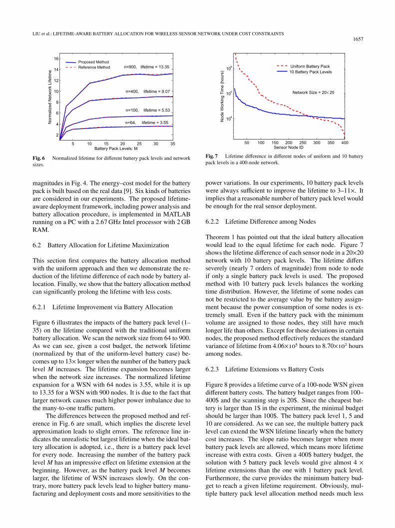
Fig. 6 Normalized lifetime for different battery pack levels and networksizes.

magnitudes in Fig. 4. The energy–cost model for the batterypack is built based on the real data [9]. Six kinds of batteriesare considered in our experiments. The proposed lifetime-aware deployment framework, including power analysis andbattery allocation procedure, is implemented in MATLABrunning on a PC with a 2.67 GHz Intel processor with 2 GBRAM.

6.2 Battery Allocation for Lifetime Maximization

This section first compares the battery allocation methodwith the uniform approach and then we demonstrate the re-duction of the lifetime difference of each node by battery al-location. Finally, we show that the battery allocation methodcan significantly prolong the lifetime with less costs.

6.2.1 Lifetime Improvement via Battery Allocation

Figure 6 illustrates the impacts of the battery pack level (1–35) on the lifetime compared with the traditional uniformbattery allocation. We scan the network size from 64 to 900.As we can see, given a cost budget, the network lifetime(normalized by that of the uniform-level battery case) be-comes up to 13× longer when the number of the battery packlevel M increases. The lifetime expansion becomes largerwhen the network size increases. The normalized lifetimeexpansion for a WSN with 64 nodes is 3.55, while it is upto 13.35 for a WSN with 900 nodes. It is due to the fact thatlarger network causes much higher power imbalance due tothe many-to-one traffic pattern.

The differences between the proposed method and ref-erence in Fig. 6 are small, which implies the discrete levelapproximation leads to slight errors. The reference line in-dicates the unrealistic but largest lifetime when the ideal bat-tery allocation is adopted, i.e., there is a battery pack levelfor every node. Increasing the number of the battery packlevel M has an impressive effect on lifetime extension at thebeginning. However, as the battery pack level M becomeslarger, the lifetime of WSN increases slowly. On the con-trary, more battery pack levels lead to higher battery manu-facturing and deployment costs and more sensitivities to the

Fig. 7 Lifetime difference in different nodes of uniform and 10 batterypack levels in a 400-node network.

power variations. In our experiments, 10 battery pack levelswere always sufficient to improve the lifetime to 3–11×. Itimplies that a reasonable number of battery pack level wouldbe enough for the real sensor deployment.

6.2.2 Lifetime Difference among Nodes

Theorem 1 has pointed out that the ideal battery allocationwould lead to the equal lifetime for each node. Figure 7shows the lifetime difference of each sensor node in a 20×20network with 10 battery pack levels. The lifetime differsseverely (nearly 7 orders of magnitude) from node to nodeif only a single battery pack levels is used. The proposedmethod with 10 battery pack levels balances the workingtime distribution. However, the lifetime of some nodes cannot be restricted to the average value by the battery assign-ment because the power consumption of some nodes is ex-tremely small. Even if the battery pack with the minimumvolume are assigned to those nodes, they still have muchlonger life than others. Except for those deviations in certainnodes, the proposed method effectively reduces the standardvariance of lifetime from 4.06×105 hours to 8.70×102 hoursamong nodes.

6.2.3 Lifetime Extensions vs Battery Costs

Figure 8 provides a lifetime curve of a 100-node WSN givendifferent battery costs. The battery budget ranges from 100–400$ and the scanning step is 20$. Since the cheapest bat-tery is larger than 1$ in the experiment, the minimal budgetshould be larger than 100$. The battery pack level 1, 5 and10 are considered. As we can see, the multiple battery packlevel can extend the WSN lifetime linearly when the batterycost increases. The slope ratio becomes larger when morebattery pack levels are allowed, which means more lifetimeincrease with extra costs. Given a 400$ battery budget, thesolution with 5 battery pack levels would give almost 4 ×lifetime extensions than the one with 1 battery pack level.Furthermore, the curve provides the minimum battery bud-get to reach a given lifetime requirement. Obviously, mul-tiple battery pack level allocation method needs much less

1658IEICE TRANS. COMMUN., VOL.E95–B, NO.5 MAY 2012

Fig. 8 Lifetime curve of a 100-node WSN under different batterybudgets.

Table 1 Time & performance comparisons between CLPS and LINGO.

Network Normalized Lifetime Execution Time (s)Size CLPS LINGO Ref CLPS LINGO36 3.22 1.93 3.26 0.004 12549 3.31 1.99 3.38 0.004 40564 3.59 3.13 3.70 0.015 1.06×105

100 5.63 N/A 5.80 0.010 N/A400 9.58 N/A 10.43 0.014 N/A900 15.11 N/A 15.59 0.067 N/A

energy budget than the uniform battery approach under thesame lifetime requirement.

6.3 Performance Comparisons with INLP Solver

As Sect. 3.1 has stated, the running time of a general-purpose INLP solver was excessive in the proposed batteryallocation procedure. We now compare the proposed algo-rithm with LINGO, a popular solver for linear and nonlin-ear programming problems. The best-case continuous node-level references are also provided to illustrate the deviationfrom the optimality. Since LINGO could not handle thenode partitioning, we do not limit the number of the batterypack types in the comparison. A branch-and-bound solverand a default iteration number are used in LINGO. The re-sults are listed in Table 1.

For the settings in Table 1, the proposed CLPS methodgains a speedup of up to 2–5 orders of magnitudes overLINGO. Furthermore, our approach can solve the batteryenergy allocation problem for a WSN with 400 nodes in lessthan 0.02 seconds while LINGO fails to find the local opti-mal solutions within 24 hours. In the small cases, our ap-proach gives even better solutions than the locally optimalsolutions by LINGO; LINGO does not necessarily providethe globally optimal solutions. Our approach considers thecharacteristics of solution to reduce the search space. It maybe possible to provide LINGO other configurations to get abetter result using more execution time. However, this com-parison provides evidence that the straightforward use of ageneral-purpose INLP solver is inappropriate for the WSN

Fig. 9 WSN lifetime under power variations compared with the onewithout power variations for different battery pack levels.

Table 2 Number of nodes whose lifetime are under the original 100-node network lifetime.

Battery Pack Level 3 5 10 15 20 25 30 35Number of Nodes 7 7 12 17 21 23 25 23

battery energy allocation problem, and that the proposed so-lution rapidly produces high-quality results.

6.4 The Impact of Power Variations on Lifetime

This experiment illustrates the impact of the node’s powervariations on the lifetime. In this case, the node num-ber of the WSN is 100 and the battery budget is 400$.The battery pack level ranges from 3 to 35. We assumeeach node’s power variation qi satisfies a Gauss distributionN(qi, 0.06qi), in which a maximal 20% power deviation isobserved among 500 samples†. Given a battery pack level,the WSN lifetime are evaluated under 500 random powerprofiles and it is determined by the node with the shortestlifetime in the network.

Figure 9 showed the lifetime variations under 500 sam-ples using each battery pack level. As we can see, the aver-age lifetime is usually smaller than the original one withoutpower variations. It validates Theorem 2 experimentally.When the battery pack level is small, the lifetime presentsa better tolerance to the power variations. It is due to thefact that fewer battery pack levels lead to more energy re-dundancy for more nodes. In order to show the effects ofpower variations on each node, Table 2 gave the numberof nodes whose lifetime become smaller after consideringpower variations. As we can see, 7 nodes in a 100-nodeWSN with 3 battery pack levels becoming shorter, while the

†The power variations of each node come from many factors,such as different protocols, process variations, voltage and tem-perature variations. Reference [11] analyzed the power variationsof a sensor node with a general configuration. It showed that thepower variations approximately follow a normal distribution withthe standard deviation 6% of the average value. Though the resultsonly hold for their configuration. It should represent a typical trendfor many real sensor nodes.

LIU et al.: LIFETIME-AWARE BATTERY ALLOCATION FOR WIRELESS SENSOR NETWORK UNDER COST CONSTRAINTS1659

number of such nodes reach up to 23 with 35 battery packlevels. Those phenomena indicated that a larger battery packlevel is not guaranteed to acquire a longer lifetime due tothe node’s power variations in reality. A not very large bat-tery pack level should provide both lifetime extension andenough tolerance to the power variations.

7. Conclusions and Future Works

Low-cost battery-powered wireless sensor nodes have quitetight power budgets. Unbalanced power distributions due tothe intrinsic many-to-one traffic in WSN results in unevenbattery depletion and short lifetimes. This paper proposed afine-grained node-level battery allocation technique. It for-mulates the cost-constrained heterogenous WSN battery al-location problem as an INLP and provides a fast heuristicthat produces near-optimal solutions. Experimental resultsshow that the proposed techniques can provide 4–13× life-time improvement with no more than 10 battery pack levelscompared with the uniform approach. Furthermore, the pro-posed heuristic method gains a speedup of 2–5 times andbetter results over a popular INLP solver. The impacts ofpower variations on lifetime are also discussed and boundedin theory. Our future work includes evaluating the meth-ods in a physical sensor network system and exploiting thismethodology in other battery-powered ad-hoc networks toextend their lifetime.

Acknowledgement

The authors would like to thank Prof. Robert Dick for hishelpful suggestions. This work was supported in part by theNSFC under grant 60976032, National Science and Tech-nology Major Project under contract 2010ZX03006-003-01and High-Tech Research, Development 863 Program undercontract 2009AA01Z130 and in part by 2011 national spe-cial fund for IoT development.

References

[1] H. Long, Y. Liu, Y. Wang, R.P. Dick, and H. Yang, “Battery allo-cation for wireless sensor network lifetime maximization under costconstraints,” Proc. Int. Conf. Computer-Aided Design, pp.705–712,2009.

[2] C.Y. Chong and S.P. Kumar, “Sensor networks: Evolution, opportu-nities, and challenges,” Proc. IEEE, vol.91, pp.1247–1256, 2003.

[3] Y. Hou, Y. Shi, H. Sherali, and S. Midkiff, “Prolonging sensor net-work lifetime with energy provisioning and relay node placement,”Proc. Sensor and Ad Hoc Communications and Networks, pp.295–304, 2005.

[4] X. Wu, G. Chen, and S.K. Das, “Avoiding energy holes in wirelesssensor networks with nonuniform node distribution,” IEEE Trans.Parallel Distrib. Syst., vol.19, no.5, pp.710–720, 2008.

[5] S.R. Gandham, M. Dawande, R. Prakash, and S. Venkatesan, “En-ergy efficient schemes for wireless sensor networks with multi-ple mobile base stations,” Proc. Global Telecommunications Conf,pp.377–381, 2003.

[6] E. Oyman and C. Ersoy, “Multiple sink network design problem inlarge scale wireless sensor networks,” Proc. International Commu-nications Conf., pp.3663–3667, 2004.

[7] M. Sichitiu and R. Dutta, “Benefits of multiple battery levels forthe lifetime of large wireless sensor networks,” Proc. Networking,pp.1440–1444, 2005.

[8] H. Long, Y. Liu, X. Fan, R. Dick, and H. Yang, “Energy-efficientspatially-adaptive clustering and routing in wireless sensor net-works,” Proc. Design, Automation & Test in Europe Conf, pp.1267–1272, 2009.

[9] “Guidelines for battery packs,” http://www.powerstream.com/BPD.htm

[10] R. Min and A. Chandrakasan, “A framework for energy-scalablecommunication in high-density wireless networks,” Proc. Int. Symp.Low Power Electronics & Design, pp.36–41, 2002.

[11] T. Matsuda, T. Takeuchi, H. Yoshino, M. Ichien, S. Mikami,H. Kawaguchi, C. Ohta, and M. Yoshimoto, “A power-variationmodel for sensor node and the impact against life time of wirelesssensor networks,” Proc. Communications and Electronics, pp.106–111, 2006.

Appendix A

Proof 1: For a given node partition L, there is anenergy partition E which divides Econs into Eset{1}, Eset{2},. . . , Eset{M}, each corresponds to a node set Li, i =1, 2, . . . ,M. The energy partition E ensures the lifetimelongest by satisfying

Eset{i}Econs

=gi · Ni∑M

k=1(gk · Nk), i = 1, 2, . . . ,M (A· 1)

The following paragraphs will prove this is true.The energy allocation E satisfies Eq. (A· 1) has the fol-

lowing property: In each Li, the lifetime Ti is:

Ti =Eset{i}gi · Ni

=Econs · gi · Ni

gi · Ni ·∑Mk=1(gk · Nk)

=Econs∑M

k=1(gk · Nk)(A· 2)

Ti is unrelated to i, that means the lifetime of each nodeset Li is equal. Furthermore, any energy partition E whichobeys this property satisfies Eq. (A· 1), because for any s andt, we get:

Eset{s}gs · Ns

=Eset{t}gt · Nt

=Econs∑M

k=1(gk · Nk)(A· 3)

Therefore, Eq. (A· 2) is the necessary and sufficient condi-tion of Eq. (A· 1).

Suppose that there is another energy partition E’, whichdoesn’t assure the equal lifetime of each L′i property. Therenecessarily exist two sets L′s and L′t such as T ′s < T ′t ≤T ′k, (k � s, t). That means T ′s is the minimum lifetime ofall the L′i . From Eq. (1), we get:

E′set{s}g′s · N′s

<E′set{t}g′t · N′t

(A· 4)

If a tiny adjustment is made on E′set{s} and E′set{t} by δ, thefollowing inequality is still satisfied:

E′set{s} + δ

g′s · N′s<

E′set{t} − δg′t · N′t

(A· 5)

1660IEICE TRANS. COMMUN., VOL.E95–B, NO.5 MAY 2012

So, the minimum lifetime of all the L′i turns a little higher.That means the energy partition E’ is not the best one.

By now, we have proved that for any node partition L,the best energy partition makes the lifetime in each Li equiv-alent. The longest network lifetime is as Eq. (5) describes.

�

Appendix B

Proof 2: Assume only the most power consuming nodewithout considering power variations in each partitioned set{xi}, i = 1, 2, . . .M can affect the network lifetime, whereM stands for the number of battery levels. We denote thedecreasing probability of lifetime as pdec and the increasingor unchanging probability as pinc. In real cases, we needremove the assumption to obtain the real decreasing proba-bility of lifetime pdec,real and the increasing or unchangingprobability pinc,real. Since any nodes may decrease the net-work lifetime and the boundary-node case is a subset, thefollowing equations hold:

pdec,real ≥ pdec (A· 6)

pinc,real = 1 − pdec,real ≤ pinc (A· 7)

Without losing generality, we assume all β j ≤ 1− δ, δ > 0 inEqs. (13) and (14), the following equations hold when M >log1−δ(0.5),

pinc = ΠMi=1βxi < (1 − δ)log1−δ(0.5) = 0.5 (A· 8)

pdec = 1 − pinc > 0.5 > pinc (A· 9)

Therefore, when M is larger enough, we have:

pinc,real ≤ pinc < pdec ≤ pdec,real (A· 10)

Assuming an unbalance distribution with δ = 0.1, β =0.9, α = 0.1, pdec > pinc when M > 7. Given a normaldistribution, we can observe pdec � pinc when M ≥ 10,.

Yongpan Liu was born in Henan Prov-ince, P.R. China. He received his B.S., M.S.and Ph.D. degrees from Electronic Engineer-ing Department, Tsinghua University in 1999,2002, and 2007. He worked as a research fel-low in Tsinghua University from 2002 to 2004.Since 2007, he became an assistant professorin Tsinghua University. He has published over40 peer-reviewed conference and journal papers,supported by NSFC, 863, 973 Program. Hismain research interests include embedded sys-

tems, nonvolatile computing, power-aware architecture and VLSI designand electronic design automation. He is an IEEE, member and served as areviewer of several IEEE conferences and TVLSI.

Yiqun Wang was born in Hubei Province.He received his B.S. from Electronic Engineer-ing Department, Tshinghua University in 2009and now is a Ph.D. student in the same depart-ment. His main research interets are low powerVLSI designs and non-volatile memory and cir-cuits. He is now working in the project of wire-less sensor network SOC design.

Hengyu Long was born in Guizhou Prov-ince, P.R. China. He was a master student inthe Department of Electronic Engineering, Ts-inghua University. His main research interestsare power-efficient protocols for wireless sensornetwork.

Huazhong Yang was born in Sichuan Prov-ince, P.R. China, on Aug. 18, 1967. He re-ceived B.S., M.S., and Ph.D. Degrees in Elec-tronic Engineering from Tsinghua University,Beijing, in 1989, 1993, and 1998, respectively.Now, he is a Professor and Head of the In-stitute of Circuits and Systems in ElectronicEngineering Department, Tsinghua University,Beijing. His research interests include CMOSradio-frequency integrated circuits, VLSI sys-tem structure for digital communications and

media processing, wireless sensor network, low-voltage and low-power cir-cuits, and computer-aided design methodologies for system integration. Hehas authored and co-authored over 30 patents, 7 books, and over 200 jour-nal and conference papers. He was granted National Palmary Young Re-searcher Fund of China.