LIFE CYCLE ENERGY ASSESSMENT OF ALTERNATIVE WATER SUPPLY ...€¦ · OF ALTERNATIVE WATER SUPPLY...

Energy Research and Development Div is ion FINAL PROJECT REPORT

LIFE‐CYCLE ENERGY ASSESSMENT OF ALTERNATIVE WATER SUPPLY SYSTEMS IN CALIFORNIA

MARCH 2011CEC ‐500 ‐2013 ‐037

Prepared for: California Energy Commission Prepared by: University of California, Berkeley Department of Civil and Environmental Engineering

PREPARED BY: Primary Author(s): Arpad Horvath Jennifer Stokes University of California, Berkeley Department of Civil and Environmental Engineering 215 McLaughlin Hall Berkeley, CA 94720-1712 510-642-7300 Contract Number: 500-02-004 Work Authorization MR-048 Prepared for: California Energy Commission Joe O’Hagan Contract Manager Linda Spiegel Office Manager Energy Generation Research Office Laurie ten Hope Deputy Director ENERGY RESEARCH AND DEVELOPMENT DIVISION Robert P. Oglesby Executive Director

DISCLAIMER This report was prepared as the result of work sponsored by the California Energy Commission. It does not necessarily represent the views of the Energy Commission, its employees or the State of California. The Energy Commission, the State of California, its employees, contractors and subcontractors make no warranty, express or implied, and assume no legal liability for the information in this report; nor does any party represent that the uses of this information will not infringe upon privately owned rights. This report has not been approved or disapproved by the California Energy Commission nor has the California Energy Commission passed upon the accuracy or adequacy of the information in this report.

i

ACKNOWLEDGEMENTS

The project team would like to acknowledge the following people who provided information and guidance to made this research possible: Joe O’Hagan of the California Energy Commission, the California Institute of Energy and the Environment, Kara Nelson of the University of California, Berkeley, and all the individuals that cooperated with the research team to provide case study information at the unidentified water and wastewater utilities. In addition, the authors would like to thank the Orange County Water District for allowing the use of their facilities to host a workshop about this research.

ii

PREFACE

The California Energy Commission Energy Research and Development Division supports public interest energy research and development that will help improve the quality of life in California by bringing environmentally safe, affordable, and reliable energy services and products to the marketplace.

The Energy Research and Development Division conducts public interest research, development, and demonstration (RD&D) projects to benefit California.

The Energy Research and Development Division strives to conduct the most promising public interest energy research by partnering with RD&D entities, including individuals, businesses, utilities, and public or private research institutions.

Energy Research and Development Division funding efforts are focused on the following RD&D program areas:

• Buildings End‐Use Energy Efficiency

• Energy Innovations Small Grants

• Energy‐Related Environmental Research

• Energy Systems Integration

• Environmentally Preferred Advanced Generation

• Industrial/Agricultural/Water End‐Use Energy Efficiency

• Renewable Energy Technologies

• Transportation

Life‐Cycle Energy Assessment of Alternative Water Supply Systems in California is the final report for the Life‐Cycle Energy Assessment of Alternative Water Supply Systems in California – Extensions and Refinements project (Contract Number 500‐02‐004, Work Authorization MR‐048) conducted by the University of California, Berkeley. The information from this project contributes to Energy Research and Development Division’s Energy‐Related Environmental Research Program.

For more information about the Energy Research and Development Division, please visit the Energy Commission’s website at www.energy.ca.gov/research/ or contact the Energy Commission at 916‐327‐1551.

iii

ABSTRACT

Providing water and wastewater services in California is often energy‐intensive. The need for alternative water sources (for example, from desalination) and tougher regulations on wastewater utilities lead to higher energy and resource requirements. The environmental implications of these services should be incorporated into design and planning decisions to develop a more environmentally responsible water and wastewater system.

Life‐cycle assessment is a quantitative, comprehensive method used in this research to account for energy consumption and environmental emissions caused by extracting raw materials, manufacturing, transporting, constructing, operating, maintaining, and decommissioning infrastructure and to incorporate these implications in decision‐making. In this research, life‐cycle assessment was used to evaluate water and wastewater systems in California by 1) creating and revising pubically available decision‐support softwares, the Water‐Energy Sustainability Tool and Wastewater‐Energy Sustainability Tool, useful to utilities and other industry professionals to evaluate their design and planning alternatives, and 2) evaluating case studies to determine the factors and parameters that affect the systems’ energy use and environmental effects. Results were reported for the life‐cycle phases, system functions, and activities. The tools created are available for public release.

The study results showed and quantified that:

• Including the life‐cycle effects of electricity generation, rather than just direct (for example, smokestack) emissions can make a significant difference in the outcomes.

• Desalination, particularly of seawater, is the most environmentally burdensome water supply alternative.

• Certain conservation programs have lower life‐cycle energy use compared to available water supply.

• Wastewater systems can significantly reduce their greenhouse gas emissions by recovering methane from their treatment process to generate electricity.

• Both water and wastewater systems exhibit economies of scale in their treatment processes.

• Results for both water and wastewater systems are site‐specific.

Keywords: Life‐cycle assessment, water supply, wastewater, energy end‐use, desalination, recycled water

Please use the following citation for this report:

Horvath, Arpad; Stokes, Jennifer. (University of California, Berkeley). 2011. Life‐Cycle Energy Assessment of Alternative Water Supply Systems in California. California Energy Commission. Publication Number: CEC‐500‐2013‐037.

iv

TABLE OF CONTENTS

Acknowledgements ................................................................................................................................... i

PREFACE ................................................................................................................................................... ii

ABSTRACT .............................................................................................................................................. iii

TABLE OF CONTENTS ......................................................................................................................... iv

LIST OF FIGURES ................................................................................................................................ viii

LIST OF TABLES ...................................................................................................................................... x

EXECUTIVE SUMMARY ........................................................................................................................ 1

Introduction ........................................................................................................................................ 1

Purpose ................................................................................................................................................ 2

Objectives ............................................................................................................................................ 2

Conclusions and Recommendations ............................................................................................... 3

Benefits to California ......................................................................................................................... 5

CHAPTER 1: Introduction ...................................................................................................................... 7

1.1 Problem Significance ................................................................................................................. 7

1.2 Problem Background ............................................................................................................... 10

1.3 Project Overview ...................................................................................................................... 11

1.3.1 Tools ................................................................................................................................... 12

1.3.2 Articles and Presentations .............................................................................................. 12

1.4 Literature Review ..................................................................................................................... 13

1.4.1 Life‐cycle Assessment ...................................................................................................... 13

1.4.2 Water and Wastewater Life‐cycle Assessment ............................................................ 14

1.5 Structure of Report ................................................................................................................... 16

CHAPTER 2: Task 2 – Assess Alternative Energy Sources ............................................................. 17

2.1 Task 2 Approach ...................................................................................................................... 17

2.1.1 Revisions ........................................................................................................................... 17

2.1.2 Case Study Description ................................................................................................... 18

2.2 Task 2 Outcomes ...................................................................................................................... 19

v

2.3 Task 2 Conclusions and Recommendations ......................................................................... 20

CHAPTER 3: Task 3 – Consider Additional Water Sources ........................................................... 21

3.1 Task 3 Approach ...................................................................................................................... 21

3.1.1 Revisions ........................................................................................................................... 21

3.1.2 Case Study Description ................................................................................................... 21

3.2 Task 3 Outcomes ...................................................................................................................... 21


CHAPTER 4: Task 4 – Calculate Emission Factors for Common Materials ................................. 27

4.1 Task 4 Approach ...................................................................................................................... 27

4.1.1 Pipe Analysis Approach .................................................................................................. 27

4.1.2 Tank Analysis ................................................................................................................... 28

4.2 Task 4 Outcomes ...................................................................................................................... 29

4.2.1 Pipe Analysis Outcomes ................................................................................................. 29

4.2.2 Tank Analysis Outcomes ................................................................................................ 33


CHAPTER 5: Task 5 – Include Life‐Cycle Effects of Electricity Generation ............................... 37

5.1 Task 5 Approach ...................................................................................................................... 37

5.1.1 Life‐cycle Electricity Approach ...................................................................................... 37

5.1.2 Sludge Disposal ................................................................................................................ 41

5.1.3 Case Studies ...................................................................................................................... 43

5.2 Task 5 Outcomes ...................................................................................................................... 43


CHAPTER 6: Task 6 – Evaluate Demand Management and Conservation Measures ............... 49

6.1 Task 6 Approach ...................................................................................................................... 50

6.1.1 Indoor Demand Management Approach ..................................................................... 53

6.1.2 Commercial, Industrial, and Institutional Demand Management Approach ......... 59

6.1.3 Outdoor Demand Management ..................................................................................... 60

6.2 Task 6 Outcomes ...................................................................................................................... 65

vi

6.2.1 Indoor Demand Management Results .......................................................................... 65

6.2.2 Indoor CII Demand Management Results .................................................................... 70

6.2.3 Outdoor demand management results ......................................................................... 70


6.3.1 Indoor Demand Management Conclusions ................................................................. 75

6.3.2 Indoor CII Demand Management Conclusions ........................................................... 76

6.3.3 Outdoor Demand Management Conclusions .............................................................. 76

CHAPTER 7: Task 7 – Consider Additional Pollutants ................................................................... 77

7.1 Task 7 Approach ...................................................................................................................... 77

7.1.1 Revisions ........................................................................................................................... 77

7.1.2 Case Study ......................................................................................................................... 79

7.2 Task 7 Outcomes ...................................................................................................................... 81


7.3.1 Revisions ........................................................................................................................... 83

7.3.2 Case Study ......................................................................................................................... 83

CHAPTER 8: Task 8 – Develop Workshops for Industry Professionals ...................................... 85

8.1 Task 8 Approach ...................................................................................................................... 85

8.2 Task 8 Outcomes ...................................................................................................................... 85


CHAPTER 9: Task 9 – Improve Material Production Analysis ...................................................... 87

9.1 Task 9 Approach ...................................................................................................................... 87

9.1.1 Revisions ........................................................................................................................... 87

9.1.2 Case Studies ...................................................................................................................... 87

9.2 Task 9 Outcomes ...................................................................................................................... 90

9.2.1 Revisions ........................................................................................................................... 90

9.2.2 Case Studies ...................................................................................................................... 90


CHAPTER 10: Task 10 – Analyze the Energy Demand of Wastewater Systems ......................... 97

vii

10.1 Task 10 Approach .................................................................................................................... 97

10.1.1 The Wastewater‐Energy Sustainability Tool ................................................................ 97

10.1.2 Wastewater Case Study ................................................................................................. 110

10.1.3 Hypothetical Case Study ............................................................................................... 113

10.2 Task 10 Outcomes .................................................................................................................. 113

10.2.1 Case Study Results ......................................................................................................... 113

10.2.2 Hypothetical System Results ........................................................................................ 116

10.3 Task 10 Conclusions and Recommendations ..................................................................... 117

10.3.1 WWEST ............................................................................................................................ 117

10.3.2 Case Studies .................................................................................................................... 118

10.3.3 General ............................................................................................................................. 118

CHAPTER 11: Task 11 – Evaluate Decentralized Water and Wastewater Systems ................. 120

11.1 Task 11 Approach .................................................................................................................. 120

11.1.1 Revisions ......................................................................................................................... 121

11.1.2 Case Studies .................................................................................................................... 121

11.2 Task 11 Outcomes .................................................................................................................. 124

11.2.1 Stonehurst Outcomes ..................................................................................................... 124

11.2.2 Corona Outcomes ........................................................................................................... 130

11.2.3 Point‐of‐Entry Outcomes .............................................................................................. 135

11.3 Task 11 Conclusions and Recommendations ..................................................................... 140

CHAPTER 12: Project Summary ....................................................................................................... 141

12.1 Project Outcomes .................................................................................................................... 142

12.1.1 Deliverables..................................................................................................................... 142

12.1.2 Water System Case Studies ........................................................................................... 143

12.1.3 Wastewater System Case Studies ................................................................................ 145

12.2 Project Conclusions ................................................................................................................ 145

12.2.1 Tools ................................................................................................................................. 145

12.2.2 Case Studies .................................................................................................................... 146

viii

12.3 Project Recommendations ..................................................................................................... 147

GLOSSARY ............................................................................................................................................ 149

REFERENCES ........................................................................................................................................ 152

LIST OF FIGURES Figure 1: Production Potential and Costs for New California Water Supply ................................... 8

Figure 2: LCA Inventory Analysis Framework ................................................................................... 14

Figure 3: Results by Water Supply Phase ............................................................................................. 22

Figure 4: Material Production Results by Material ............................................................................. 23

Figure 5: WESTLite Pipe Data Entry Worksheet ................................................................................. 28

Figure 6: Tank Analysis Data Entry Worksheet .................................................................................. 29

Figure 7: Pipe Analysis Results Worksheet – Summary Results ....................................................... 30

Figure 8: Energy Use Results for 100 feet of Pipe ................................................................................ 32

Figure 9: Tank Analysis Results Worksheet ......................................................................................... 33

Figure 10: Results Summary for 10 MG of Storage ............................................................................. 36

Figure 11: Energy Mix Data Entry Page ................................................................................................ 39

Figure 12: Comparison of SC and NC Results ..................................................................................... 44

Figure 13: Activity Contribution to GHG and NOx Results ............................................................... 45

Figure 14: Life‐cycle Phase Results for Utilities ................................................................................... 46

Figure 15: Water Supply Phase Results for Utilities ........................................................................... 46

Figure 16: Evapotranspiration Superzones .......................................................................................... 61

Figure 17: Potential Savings Statewide of Indoor Demand Management Fixtures ........................ 75

Figure 18: Desalination Results by Activity ......................................................................................... 82

Figure 19: Desalination Results Comparison ....................................................................................... 84

Figure 20: NC‐Large System Energy Results by Life‐cycle Phase .................................................... 91

Figure 21: NC‐Large System Energy Results by Water Supply Phase ............................................. 91

Figure 22: NC‐Large Reservoir Energy Results by Water Supply Phase ......................................... 92

Figure 23: NC‐Large System Energy Results by Activity................................................................... 93

ix

Figure 24: NC‐Small System Energy Results by Life‐cycle Phase ..................................................... 94

Figure 25: NC‐Small System Energy Results by Water Supply Phase ............................................. 95

Figure 26: NC‐Small System Energy Results by Activity ................................................................... 95

Figure 27: Research Boundaries ............................................................................................................. 98

Figure 28: General Information Data Entry Worksheet .................................................................... 101

Figure 29: WWEST Sample Results Data Worksheet ........................................................................ 107

Figure 30: WWEST Sample Results Graphs Worksheet ................................................................... 108

Figure 31: WWTP Process Diagram .................................................................................................... 111

Figure 32: Greenhouse Gas Emissions by Activity ........................................................................... 115

Figure 33: Decentralized Wastewater Treatment System for the Stonehurst Case Study ........... 122

Figure 34: Decentralized Wastewater Treatment System for the Corona Case Study ................. 123

Figure 35: Point‐of‐Entry Water Treatment Case Study ................................................................... 123

Figure 36: Energy and GHG Emissions Summary ............................................................................ 124

Figure 37: Water Supply Phase Energy Use ....................................................................................... 125

Figure 38: Life‐Cycle Phase Energy Use ............................................................................................. 125

Figure 39: Activity Phase Energy Use ................................................................................................. 126

Figure 40: Water Supply Phase GHG Emissions ............................................................................... 127

Figure 41: Life‐Cycle Phase GHG Emissions ..................................................................................... 127

Figure 42: GHG Emissions by Activity ............................................................................................... 128

Figure 43: Air Pollutant Emissions Summary .................................................................................... 128

Figure 44: Water Supply Phase Air Pollutant Emissions ................................................................. 129

Figure 45: Life‐Cycle Phase Air Pollutant Emissions ........................................................................ 130

Figure 46: Air Pollutant Emissions by Activity ................................................................................. 130

Figure 47: Treatment Phase Energy and GHGs Summary ............................................................... 131




Figure 51: GHG Emissions by Activity ............................................................................................... 133

x

Figure 52: Treatment Phase Air Pollutant Emissions Summary ..................................................... 134



Figure 55a and 55b: Water Treatment Energy and GHGs Summary ............................................. 136




Figure 59: GHG emissions by Activity ................................................................................................ 138

Figure 60: Water Treatment Air Pollutant Emissions Summary ..................................................... 139



Figure 63: Comparison of Energy Demand of Various Water Sources .......................................... 144

LIST OF TABLES Table 1: Water LCA Literature Summary ............................................................................................. 15

Table 2: Summary of Wastewater LCA Literature .............................................................................. 16

Table 3: Desalination Scenario Descriptions ........................................................................................ 19

Table 4: Desalination Scenario Results .................................................................................................. 19

Table 5: Summary of Results for the Water Sources Comparison Study ......................................... 22

Table 6: Electricity Consumption Estimates for the Northern California Utility ............................ 24

Table 7: Source Results for Revised Electricity Use ............................................................................ 24

Table 8: Results for Current Utility Water Mix (importation, no desalination) .............................. 25

Table 9: Results for Proposed Utility Water Mix (desalination, no importation) ........................... 25

Table 10: Emission Factors per 100 feet of Pipe ................................................................................... 31

Table 11: Data Analysis for 24‐in. and 36‐in. Pipe ............................................................................... 32

Table 12: Tank Scenario Summary ........................................................................................................ 34

Table 13: Tank Scenario Emission Factors ............................................................................................ 35

Table 14: Tank Scenario Component Energy Results ......................................................................... 35

xi

Table 15: Life‐cycle Emission Factors by Generation Type for California ....................................... 38

Table 16: Emission Factors per kilowatt‐hour by Generation Technology ...................................... 40

Table 17: Emission Factors per kilowatt‐hour by Geographic Location .......................................... 41

Table 18: Sludge Disposal Emission Factors ........................................................................................ 42

Table 19: Emissions per functional unit for each source and system ............................................... 43

Table 20: Summary of Conservation Potential ..................................................................................... 50

Table 21: EIO‐LCA Emission Factors by Sector ................................................................................... 51

Table 22: External Cost Estimates .......................................................................................................... 52

Table 23: Summary of Indoor Water Use ............................................................................................. 53

Table 24: Aquacraft Studies Summary .................................................................................................. 54

Table 25: Toilet Performance Data ......................................................................................................... 55

Table 26: Showerhead Performance Data ............................................................................................. 56

Table 27: Faucet Performance Data ....................................................................................................... 57

Table 28: Washing Machine Performance Data ................................................................................... 59

Table 29: Office Building Fixture Details .............................................................................................. 60

Table 30: Outdoor Water Use Scenarios ............................................................................................... 63

Table 31: NC Supply Environmental and Economic Result Summary ............................................ 66

Table 32: Environmental Effects of Indoor Residential Material Production .................................. 67

Table 33: Economic Impacts of Water Conservation .......................................................................... 69

Table 34: Environmental Effects and Total Economic Cost Results for Office Building ................ 70

Table 35: Environmental Impacts of Outdoor Water Conservation ................................................. 71

Table 36: Environmental Effects of Outdoor System Material Production ...................................... 73

Table 37: Household/Facility Economic Impacts of Outdoor Water Conservation ....................... 74

Table 38: Air Emission Factors added to WEST and WWEST ........................................................... 78

Table 39: Water Emission Factors Added to WEST and WWEST ..................................................... 79

Table 40: Water Production for Three Cities ........................................................................................ 80

Table 41: Ocean Desalination Case Study Details ............................................................................... 80

Table 42: Desalination Energy and Air Emission Results .................................................................. 81

xii

Table 43: Expanded Land and Air Emissions Results ........................................................................ 82

Table 44: Water Emissions Results ........................................................................................................ 83

Table 45: NC‐Large Case Study Summary ........................................................................................... 88

Table 46: NC‐Small Case Study Summary ........................................................................................... 89

Table 47: NC‐Large Results Summary for Sources and System ........................................................ 90

Table 48: NC‐Small Results Summary for Sources and System ........................................................ 93

Table 49: LCA System Boundaries ......................................................................................................... 99

Table 50: WWEST Material Summary ................................................................................................. 105

Table 50: Annual Liquid and Sludge Volume Processed ................................................................. 110

Table 52: Annual Treatment Chemical Consumption ...................................................................... 112

Table 53: Annual Energy Consumption Summary ........................................................................... 112

Table 54: Fleet Vehicle Summary ......................................................................................................... 113

Table 55: Wastewater Utility Energy Use and Air Emission Results ............................................. 114

Table 56: Project Deliverables ............................................................................................................... 142

Table 57: Project Case Study Summary............................................................................................... 143

Table 58: California Utility Results Summary .................................................................................... 143

Table 59: Wastewater Case Study Summary ...................................................................................... 145

Table 60: Wastewater Case Study Summary (treatment only) ........................................................ 145

1

EXECUTIVE SUMMARY

Introduction Water and energy are interconnected. Prior research has shown that the energy required for water processing contributes significantly to water’s environmental effects. Worldwide, pumping and treating urban water and wastewater consume as much as three percent of energy, which will only increase as population and demand for better treatment and sanitation increase. In California, water‐related services use significant portions of the state’s electricity and natural gas. Energy use will grow as desalination or other energy‐intensive sources are adopted in water‐scarce areas. Growth in desalination will come at considerable energy and environmental costs.

The environmental impacts of wastewater are also of concern. Changes in regulations on wastewater discharge requirements may increase the associated energy use. Wastewater treatment plants are regulated to limit their impact on the environment; however, regulations focus on chemical concentrations in liquid outflow and solid waste. They rarely consider the broader effects associated with the wastewater system’s life cycle, including material production and use, infrastructure construction and maintenance, and energy production impacts. But the regulatory landscape is changing; for example, recent California legislation, the Global Warming Solutions Act of 2006 (Núñez, Chapter 488, Statutes of 2006), regulates greenhouse gas emissions associated with wastewater treatment plants.

While rarely considered, the environmental effects of material and energy intensity should complement conventional design criteria when making water utility decisions. Infrastructure construction and maintenance as well as material production and delivery contribute to energy use and the overall impacts, or “environmental burden.” The energy and materials used and the construction processes needed to install this infrastructure also increase a utility’s life‐cycle environmental effects. Desalination plants, for example, are being considered by some coastal California utilities to provide a reliable and local water source. Adding solar power capacity is assumed to reduce greenhouse gas emissions, without considering the emissions created during the manufacturing, installation, operation, and decommissioning of solar photovoltaic or concentrated solar power plants.

The tool described in this report uses a life‐cycle assessment framework that allows a utility to compare the resulting greenhouse gas emissions in their decision process more comprehensively. Life‐cycle assessments evaluate the environmental effects associated with all stages, from original material extraction, material processing, manufacturing, distribution, use, maintenance, and disposal. The life‐cycle assessment framework presented in this report can also evaluate many other systemwide or process‐specific decisions, such as selecting pipe materials, filters (conventional vs. membrane), disinfection processes, or different operational strategies.

Water and wastewater services are necessary for healthy life and will be provided even when the best available alternative is costly, but system planners should strive to select options that

2

minimize energy and material use and the associated environmental effects from the use of these resources.

Purpose The research described in this report is an enhancement and expansion of an earlier method to analyze the energy and environmental effects associated with water supply infrastructure. This earlier study, by the same authors of this report, is titled Life‐cycle Energy Assessment of Alternative Water Supply Systems in California and is available on the Energy Commission website at http://www.energy.ca.gov/pier/project_reports/CEC‐500‐2005‐101.html. The original project was a broad‐scope, screening‐level analysis of water supply infrastructure that developed and used the Water Energy Sustainability Tool. The initial study sought to identify the most important parameters for such assessments and to provide focus for more detailed analyses. Therefore, the research described herein is intended to refine and expand the original work by making it more comprehensive, precise, and robust, as well as adding case studies to demonstrate the utility of such an approach.

This research provides additional information that can be used by water and wastewater utilities and other industry professionals to improve design, planning and operational decisions for these public services. Two Microsoft Excel®‐based decision support tools, the revised Water‐Energy Sustainability Tool and the new Wastewater‐Energy Sustainability Tool, are provided to allow users to calculate the life‐cycle energy and environmental implications of infrastructure associated with California’s water and wastewater systems.

Objectives The objectives of this project are to:

• Revise the Water Energy Sustainability Tool to assess alternative energy sources and custom energy mixes, including options for renewable energy from solar, wind, and biomass sources.

• Update the Water Energy Sustainability Tool to analyze other scenarios (for example, groundwater, surface water, or alternative treatment processes) or alternative scenarios (such as using chlorine versus ultraviolet disinfection).

• Create a simplified tool that will calculate emission factors for common materials in water and wastewater systems such as pipe materials and tank design.

• Improve the Water Energy Sustainability Tool to include the life‐cycle effects of electricity generation that accounts for the effects of mining, processing, and transporting fuel from its source to the point of combustion, and manufacturing and transporting all associated equipment.

• Evaluate demand management measures and compare them to water supply alternatives.

• Revise the Water Energy Sustainability Tool to consider additional air pollutants as well as water and land pollutants.

3

• Create a tool to analyze the energy demand of wastewater systems (Wastewater‐Energy Sustainability Tool).

• Develop workshops for industry professionals.

• Improve material production analysis of certain materials that were not well‐defined in the original tools, especially chemicals and plastics.

• Evaluate decentralized water and wastewater systems.

• Evaluate case studies to demonstrate the capabilities of Water Energy Sustainability Tool and the Wastewater Energy Sustainability Tool.

Conclusions and Recommendations The project conclusions are presented in the following. Regarding the tools themselves:

• The Water‐Energy Sustainability Tool has been revised to allow significantly more customization. Changes include allowing custom mixes of electricity generation sources, customizing the water sources or process scenarios that can be analyzed, adding the sludge disposal activity, and including emission factors for additional air, water, and land emissions.

• The Wastewater‐Energy Sustainability Tool allows users to analyze wastewater systems using a life‐cycle assessment perspective. The tool was designed to be more user‐friendly than the Water‐Energy Sustainability Tool. In particular, the Wastewater‐Energy Sustainability Tool contains many default assumptions so users do not need as much detailed data to get a basic assessment of their treatment process. However, results will be improved if data entry is complete, accurate, and detailed.

None of the tools assess all environmental emissions, account for ecological effects, or quantify environmental impacts such as human toxicity. For water systems, it does not address the sustainability of supply (ensuring that recharge is equal to or greater than withdrawals). Though the assessment of sustainability for water and wastewater system is not complete, it does fill a gap by allowing utilities to capture an element of environmental sustainability that has been previously ignored.

Regarding the case study analyses:

• When small‐scale decisions about pipes and tanks are analyzed, steel pipe and tanks tend to be environmentally preferable over other materials (for example, concrete and plastic).

• Custom electricity mixes, including additional renewable energy, can improve the environmental performance of water and wastewater systems. However, the impacts of renewable, or green, energy sources (for example, solar, wind, geothermal) are not zero, as is often assumed, if one includes the life‐cycle impacts of the manufacture and transport of equipment for electricity generation.

• Sludge disposal tends to have little impact on the results for water and wastewater utilities. However, the disposal choice is one way that utilities can create “negative emissions”

4

(emission savings) for greenhouse gases and other air pollutants. Selecting landfills for disposal that use gas to produce electricity or incinerators with energy or heat recovery can reduce the systems’ overall environmental impact, albeit marginally.

• Wastewater system results can be significantly improved by using methane to offset other electricity supplies. The plant in the case study is able to meet approximately 90 percent of its electricity needs using captured methane.

• Demand management or conservation programs can provide an inexpensive and environmentally preferable alternative to water supply. Converting to low‐flow toilets, in particular, can provide significant savings when implemented statewide. Four strategies for conserving water outdoors are beneficial compared to water supply in this analysis: turf maintenance, xeriscaping, water pricing, and dormant turf.

• A desalination system can have a wide variety of impacts depending on the water source. In all cases, energy use is higher than alternative water supply.

• Case study results are site‐specific and will vary by geography, hydrology, system design, water sources, and other factors. The case study results in this report can be used as guidance but may not be directly applicable to other utilities.

• Centralized water and wastewater treatment plants have lower energy requirements for a given amount of treated water relative to decentralized systems compared in this report through economies of scale.

Based on the outcomes and conclusions of this work, the following recommendations can be made:

• The Water Energy Sustainability Tool and the Wastewater Energy Sustainability Tool should be introduced to utilities to educate them about the tools themselves and, perhaps more important, about life‐cycle thinking itself. Utilities should be encouraged to take a long‐term and life‐cycle perspective on energy use and emissions, including indirect emissions associated with the supply chain. Life‐cycle assessment should be encouraged for design and planning of new water and wastewater systems and major system expansions and retrofits.

• Desalination is often discussed as an alternative for coastal water systems needing a reliable water source. However, the energy and environmental effects should be accounted for in decision‐making. If implemented in several large cities, the impact of desalination on the state’s energy supplies would be significant.

• Some wastewater treatment processes allow opportunities for heat and energy recovery that can offset fossil fuel consumption and prevent or lower greenhouse gas emissions. Anaerobic treatment processes, which produce methane, are particularly good candidates that should be considered.

• Water and wastewater systems that want to limit their environmental burden should carefully evaluate disposal choices. Offsets of fuel or electricity consumption as well as other

5

materials (for example, fertilizers) can be important to limiting the system’s effect on the environment.

• Based on the interest in this research project at the two workshops conducted as part of this work to introduce industry personnel to the tools, the researchers and the California Energy Commission should try to keep the participants and other interested parties apprised of the latest research and tools available for evaluating these issues after this contract ends.

Water and wastewater design decisions are made based on several factors, including economic, engineering, and political concerns. Heretofore, the comprehensive and systemwide life‐cycle environmental effects of the water infrastructure have not been a factor in these decisions. Generally, utilities, designers, and system planners are not aware that it is possible to assess the environmental effects of their systems using life‐cycle assessment; as a result, the analysis is not included in decision‐making.

For a more comprehensive picture of the costs associated with water supply choices, life‐cycle assessment using the Water Energy Sustainability Tool, the Wastewater Energy Sustainability Tool, or similar method should be conducted routinely. This assessment would allow the industry to develop a comprehensive list of design recommendations for systems of differing parameters (for example, scale, water quality, process selection). The model and tools described in this report will allow utilities and other planners to incorporate these effects into their decision processes and strive for sustainable solutions with more informed analyses.

Benefits to California

Traditionally, the energy demand and associated environmental effects of the water infrastructure have not been a factor in water management decisions. The decision‐support tools described in this report will allow utilities and other planners to assess the comprehensive and systemwide life‐cycle consequences of alternative approaches to water management infrastructure and incorporate these effects and externalities into their decision processes, and with more informed analyses, strive for sustainable solutions.

7

CHAPTER 1: Introduction The following report describes the methods, outcomes, and recommendations of the project “Life‐cycle Energy Assessment of Alternative Water Supply Systems in California – Extensions and Refinements,” CIEE Award No. MR‐06‐08. The project was completed by researchers at the University of California, Berkeley (UC Berkeley) on behalf of the California Energy Commission (CEC) between October 15, 2006 and December 31, 2010.

Some portions of the text of this report have been previously published in a similar format in the following papers (see list of references): (Stokes and Horvath 2006), (Stokes and Horvath 2009), (Stokes and Horvath 2010), and (Stokes and Horvath 2011).

1.1 Problem Significance The scarcity of drinking water is a growing issue throughout many parts of the world, with 1.8 billion people located in areas likely to experience absolute water scarcity by 2025 (United Nations 2006). When relying solely on locally available freshwater, more than 40 percent of the world’s population may face serious water shortages (Gleick et al. 2003). This scarcity may be due to climate, lack of infrastructure, political conflicts, or a combination of reasons.

The Western United States is especially sensitive to water scarcity. California consumes over six trillion liters of water annually for urban use. With California’s population expected to grow by 14 million people by 2030, water demand will increase by 40 percent in the same period, based on 2000 water use rates (Hanak 2005). The more arid areas of the state will experience much of this growth, further exacerbating scarcity concerns (USBR 2003). Most water in arid areas is currently imported via a major conveyance network comprised of more than 4,800 km of pipelines, tunnels, and canals, and dozens of pump stations, such as the State Water Project (SWP; from the Sacramento/San Joaquin River delta) and the Colorado River Aqueduct (CRA). More than 18 percent of California’s urban water use, as well as a significant volume of water for agricultural and environmental uses, is supplied via the CRA and the SWP, both of which may be adversely affected by climate change (Christensen et al 2004, Bennet et al 2004, Venrheenen et al 2004).

When traditional water sources fail to meet demand, alternatives need to be found. The current water supply system is already energy‐ and resource‐intensive. Future alternatives will have even have higher energy and resource requirements and, consequently, environmental impacts. To develop a sustainable water system, these environmental implications should be incorporated into the water supply planning process.

Water and wastewater system sustainability incorporates a variety of considerations, including economic, engineering, social, and environmental issues. Past studies have proposed indicators for system sustainability in all categories [e.g., (Lundin and Morrison 2002; Sahely et al. 2006)]. The traditional engineering perspective only evaluates economic and engineering performance to determine system sustainability, though equity and other social issues can factor into some

8

decisions [e.g., (Calijuri et al. 2005)]. Economically, obtaining water in dry areas is already expensive and costs will increase with scarcity. For example, brackish groundwater desalination can range in cost between $110 and $1,000 per 1,000 m3 of water ($130 – $1,250 per acre‐foot [AF]), and ocean desalination can cost $650 to $1,200 per 1,000 m3 ($800 ‐ $1,500 per AF) (Hanak 2005). Figure 1 depicts costs and potential volumes available for water sources in Southern California.

Figure 1: Production Potential and Costs for New California Water Supply

Source: Hanak 2005, California DWR 2005

The social and political implications of water scarcity have been discussed (e.g., in reference [Wolf 2007]) and can include water wars and transboundary conflicts between states. In the United States, conflicts occur between water providers, e.g., between the agriculture sector and urban utilities.

Environmental assessments are typically only applied to pre‐existing environmental hazards and sensitive receptors in the area, such as human population, endangered species, and wetlands. Two major components of achieving water system environmental sustainability are often neglected. First, that water consumption occurs at or below the rate at which fresh water is returned to the source, so that these sources are not depleted. Second, the material and energy intensity of water infrastructure are minimized and can be continued long‐term. The effects of

0

0.5

1

1.5

2

2.5

3

Sur

face

sto

rage

($

120-

820)

Des

alin

atio

n ($

100-

1200

)

Rec

ycle

d w

ater

($

490)

Urb

an d

eman

d m

anag

emen

t ($

80-4

90)

Volu

me

(mill

ion

liter

s)

Source ($ per million liters)

Low estimate

High estimate

9

excessive water consumption are site‐specific, depending on climate, geography, hydrology, and ecology, and have been well discussed (e.g., [Calijuri et al. 2005; Hall et al. 2000]).

Conversely, minimizing the material and energy intensity of water infrastructure is an area of water sustainability that is more generalizable between diverse systems and provides the focus for this research.

The connection between water and energy use is strong. Water is used to produce energy (e.g., hydropower, solar thermal) and as an input to generation (e.g., cooling water). Water treatment and transport requires energy, which contributes significantly to the environmental effects of water. Pumping and treating urban water and wastewater consumes two to three percent of worldwide energy use (ASE 2002). This energy use is expected to grow by 33 percent over the next twenty‐year period, as population growth increases demand for water and sanitation services. Broadly viewed, California’s water‐related services use approximately 19 percent of the state’s electricity use and 30 percent of natural gas (CEC 2005; Navigant 2006). This energy use estimate includes aspects of water use not analyzed in this study such as agricultural water pumping and water heating by the consumer (CEC 2005). This connection, and the amount of electricity consumed, will grow as desalination or other energy intensive sources are adopted in water‐scarce areas. Worldwide, desalination is considered a realistic water source in arid, coastal regions, including California, Florida, Mediterranean islands, and the Middle East. Desalination is not without critics, however (Dickie 2007), as it incurs considerable energy and environmental cost. The electricity used to supply water is the main source of greenhouse gases (GHG) from water provision, thereby contributing to the climate change problem.

Wastewater sustainability is also a concern. Changes to wastewater discharge requirements may increase the associated energy use. While wastewater treatment plants (WWTPs) are regulated to limit their impact on the environment, these regulations primarily address chemical concentrations in liquid effluent and solid waste. The broader effects associated with the wastewater system’s life cycle are rarely considered, such as material production and use, infrastructure construction and maintenance, and energy production impacts.

Accounting for the environmental effects of material and energy intensity can inform water utility decision making when used in conjunction with conventional design criteria. While the environmental burden of infrastructure construction and maintenance as well as material production and delivery can be inconspicuous, the impact can be substantial. Water, sewer, district heating pipelines and similar infrastructure, for example, account for 10–20 percent of urban building mass (Herz and Lipkow 2002). Because the infrastructure in this country is aging, the U.S. Environmental Protection Agency (U.S. EPA) has estimated that nationwide capital spending to provide drinking water needs to be $334.8 billion over twenty years (USEPA 2009). A separate assessment estimates water and wastewater infrastructure needs an additional $107 billion in the next five years to be up‐to‐date (American Society of Civil Engineers 2009). The energy and materials used and the construction processes needed to install this infrastructure also increase a water or wastewater utility’s life‐cycle environmental effects.

10

Desalination plants, for example, are being considered by some coastal California utilities to provide a reliable and local water source. Adding solar power capacity is also being evaluated to reduce GHG emissions, without considering the emissions created upstream, during the manufacturing, installation, operation, and decommissioning of solar photovoltaic or concentrated solar power plants. The tool described in this report uses a life‐cycle assessment (LCA) framework that allows a utility to more comprehensively compare all resulting greenhouse gas emissions in their decision process. The life‐cycle assessment framework presented in this report can evaluate many other system‐wide or process‐specific decisions, such as selecting pipe materials, filters (conventional vs. membrane), disinfection processes, or different operational strategies.

Water and wastewater services are necessary for healthy life and will be provided even when the best available alternative is costly. However, system planners should aspire to minimize energy and material use and associated environmental effects. Accounting for energy and environmental effects in water planning requires LCA, a systematic methodology to account for energy and materials resource use and other environmental effects caused by extracting raw materials, manufacturing, constructing, operating, maintaining, and decommissioning the water supply infrastructure. Section 1.3 provides a more detailed discussion. Using LCA methodology, two MS Excel‐based decision support tools, the Water‐Energy Sustainability Tool (WEST) and the Wastewater‐Energy Sustainability Tool (WWEST), were created to provide calculators of the energy and environmental implications of infrastructure associated with California’s water and wastewater systems.

1.2 Problem Background The Energy Commission’s Public Interest Energy Research – Environmental Area (PIER‐EA) project, “Life‐cycle Energy Assessment of Alternative Water Supply Systems in California” CIEE Award No. MR‐03‐20 was funded in 2003‐2004 to develop a methodology to analyze the energy and environmental effects associated with water supply infrastructure. The full details of that project are reported in Commission Publication CEC‐500‐2005‐101. The original project was intended to be a broad‐scope, screening‐level analysis of water supply infrastructure. The goal of the initial study was to identify the most important parameters and provide focus for more detailed analyses. Therefore, the research proposed herein is intended to refine and expand the original work, making it more comprehensive, precise, and robust.

At the outset of the project, WEST specifically focused on three water sources: imported, recycled, and desalinated water. It analyzed the effects of four activities associated with energy and material use in infrastructure: material production, material delivery, construction and maintenance equipment use, and energy production in all life‐cycle stages of the water supply system. WEST reported life‐cycle effects in terms of gigajoules (GJ) of energy use and million grams (Mg) of air emissions, including GHGs reported in units of carbon dioxide equivalents (CO2(e)), sulfur oxides (SOx), particulate matter (PM), nitrogen oxides (NOx), volatile organic compounds (VOC), and carbon monoxide (CO). Energy use and environmental emissions were reported for the water supply alternatives, life‐cycle phases (construction, operation, and maintenance), and water supply functions (supply, treatment, and distribution). Two California

11

case study systems were evaluated using WEST as a part of the original study, the Marin Municipal Water District (MMWD) and the Oceanside Water District (OWD). Information on WEST and prior research is available in Energy Commission’s Publication 500‐2005‐10 (Stokes and Horvath 2005). Additional information about this phase of research is available in (Stokes 2004) and (Stokes and Horvath 2006). The work done prior to the start of this contract in 2006 will be referred to as Phase One work in this report.

In the following, tasks to extend, improve, and refine the water provision LCA methodology and WEST with the goal of making them more comprehensive, precise, and robust are described.

1.3 Project Overview The tasks for this project were:

• Task 1: Administration. Task 1 consisted primarily of tracking project activities, reporting, and budgeting over the project period.

• Task 2: Assess alternative energy sources. The Phase One WEST tool assumed that the state average electricity mix was used in the analysis. For Task 2, WEST was edited to allow the user to enter customized electricity mixes, including options for renewable energy from solar, wind, biomass, and geothermal sources.

• Task 3: Consider additional water sources. After Phase One, the tool allowed only analysis of imported, desalinated, and recycled water. After Task 3’s completion, the tool can be used to analyze other water sources or alternate scenarios (i.e., groundwater, surface water, or alternative treatment processes).

• Task 4: Calculate emission factors (EFs) for common materials. Task 4 evaluated the life‐cycle emissions for common material choices in water supply systems, including pipe materials and tank design.

• Task 5: Include life‐cycle effects of electricity generation. The Phase One version of WEST contained direct (i.e., smokestack) EFs for electricity use. Task 5 consisted of updating the EFs to allow the user to analyze their water systems using life‐cycle EFs for electricity production, considering the effects of mining, processing, and transporting fuel from its source to the point of combustion and manufacturing and transporting all associated equipment.

• Task 6: Evaluate demand management measures. Task 6 quantified the effects of reducing water demand through conservation programs by evaluating the life‐cycle impacts of water‐efficient fixtures and appliances, rain collection systems, common irrigation systems in residential and commercial/industrial applications.

• Task 7: Consider additional pollutants. Task 7 expanded the pollutants analyzed by WEST beyond energy use, GHGs, and certain air pollutants included in Phase One. The revised tool evaluates additional air pollutants as well as water and land pollutants.

12

• Task 8: Develop workshops for industry professionals. Task 8 involved planning and presenting WEST and WWEST to industry professionals during two workshops, one in Southern California and one in Northern California.

• Task 9: Improve material production analysis. Task 9 improved the material production analysis by providing more detailed analysis of certain materials that are not well‐defined using EIO‐LCA, especially chemicals and plastics. Data for these improvements were obtained from publically‐ and commercially‐available sources.

• Task 10: Analyze the energy demand of wastewater systems. A separate decision support tool, WWEST, was created and used to evaluate a case study system in Task 10.

• Task 11: Evaluate decentralized water and wastewater systems. WEST and WWEST were updated as needed to evaluate decentralized water and wastewater case studies. The results were compared to previously‐evaluated centralized systems.

Since many of the tasks were interrelated, several deliverables and project outcomes do not fit neatly into a single task and are summarized below.

1.3.1 Tools The final version of WEST and the associated user manual are included as Appendices A.1 and A.1.1, respectively. A list of revisions made to the tool since its original release is Appendix A.1.2. The WEST explanatory worksheets are presented in Appendix A.1.3.

The final version of WWEST and the associated user manual are included as Appendices A.2 and A.2.1, respectively. A list of revisions made to the tool since its original release is Appendix A.2.2. The WWEST Help worksheets are presented in Appendix A.2.

After publication of this report, updated versions of the tools and documentation will be available at: http://west.berkeley.edu/model.php.

1.3.2 Articles and Presentations The following articles have been published as part of the research project. Due to copyright restrictions, the full text of these articles cannot be provided for public access on the internet and are therefore not included in this report.

• Stokes, J. R. and A. Horvath (2009). ʺEnergy and Air Emission Effects of Water Supply.ʺ Environmental Science & Technology 43(8): 2680‐2687. The paper can be found at: http://pubs.acs.org/doi/abs/10.1021/es801802h

• Stokes, J. and A. Horvath (2010). ʺSupply‐chain Environmental Effects of Wastewater Utilities.ʺ Environmental Research Letters 5(1): 014015. The paper can be found at: 10.1088/1748‐9326/5/1/014015

• Stokes, J. and A. Horvath (2011). ʺ Life‐Cycle Assessment of Urban Water Provision: Tool and Case Study in California.ʺ Journal of Infrastructure Systems 17(1): 15‐24. This article can be found at: http://dx.doi.org/10.1061/(ASCE)IS.1943‐555X.0000036

13

In addition, the research was presented at several conferences. A copy of the slides used for each presentation is included in the appendix indicated.

• C. Facanha and J. Stokes (2007). “Sustainability of Infrastructure Systems.” Chinese Institute of Engineers Conference, San Jose, Calif., February 11. (Appendix B.2.1)

• J. Stokes (2007). “Life‐cycle Climate Change Effects of Water Supply Systems.” American Water Works Association (AWWA) California‐Nevada Section Conference, Sacramento, Calif., October 24. (Appendix B.2.2)

• J. Stokes (2007). “Life‐cycle Environmental Evaluation of California Water Supply.” Society for Environmental Toxicology and Chemistry ‐ North America Annual Conference, Milwaukee, Wisc., November 9. (Appendix B.2.3)

• J. Stokes (2007). “The Life‐cycle Climate Change Contributions of Water Systems.” Presented to the Peninsula AWWA Monthly Meeting, Sunnyvale, Calif., December 5. (Appendix B.2.4

• J. Stokes (2008). “Energy Use and Greenhouse Gas Emissions of Wastewater Services: A Life‐cycle View.” AWWA California‐Nevada Section Conference, Hollywood, Calif., April 24. (Appendix B.2.5)

• J. Stokes (2009). “A Cradle‐to‐Cradle Assessment of Energy and Climate Change Impacts of Recycled Water.” WateReuse California Section Conference, San Francisco, Calif., March 23. (Appendix B.2.6)

1.4 Literature Review 1.4.1 Life-cycle Assessment The methodological framework of this study was LCA, a systematic, quantitative approach to evaluating the impacts of materials, products, processes, or services from “cradle” to “grave” (Graedel and Allenby 2003; Curran 1996). LCA considers all energy and environmental implications of processes through the entire life‐cycle, including design, planning, material extraction and production, manufacturing or construction, use, maintenance, and end‐of‐life fate of the product (reuse, recycling, incineration, or landfilling). This analysis was first described by the Society for Environmental Toxicology and Chemistry (SETAC) (SETAC 1991; SETAC 1993) and refined by the U.S. EPA in 1993 (Vigon 1993). The procedure was formalized by the International Organization of Standardization (ISO) 14040 series standards (ISO 1997; ISO 1998; ISO 2004). Figure 2 presents the LCA framework (US EPA 1993).

Process‐based LCA requires data collection from various companies, government agencies, and published studies to evaluate the inputs and outputs to the system. Economic Input‐Output Analysis‐based LCA (EIO‐LCA) is an alternative matrix‐based LCA approach. It uses the U.S. Department of Commerce’s economic input‐output model and augments it with publicly available resource consumption and environmental emissions data (CMU 2005; Hendrickson et al. 1998; Hendrickson et al. 2006). As a general interdependency model, the economic input‐output model describes interactions almost 500 sectors of the economy. For an expenditure in a

14

given economic sector, the model estimates how much is spent directly in that sector, as well as in the supply chain. In addition, the model calculates environmental emissions associated with the specified expenditure. EIO‐LCA is comprehensive, considering all resource inputs and environmental emissions, and provides information on direct emissions associated with the studied process and indirect emissions occurring in the supply chain. The principal investigator has been one of developers of the EIO‐LCA model since 1995.

Figure 2: LCA Inventory Analysis Framework

Source: US EPA 1993

This research implemented a tiered hybrid LCA methodology (Suh and Huppes 2004) in this research, combining elements of process‐based LCA and EIO‐LCA. The hybridization is intended to take advantages of the strengths of each method while minimizing the disadvantages. The details of the hybridization are discussed in Chapters 9 and 10.

1.4.2 Water and Wastewater Life-cycle Assessment Previous environmental LCAs of urban water and wastewater systems are limited to specific system components or are based on systems in other countries. A process‐based LCA of the Belgian water cycle (pumping station to wastewater treatment) determined the effects of discharging untreated or marginally treated wastewater are more important than operational effects such as energy use (Lassaux et al. 2007). A second study evaluated water and wastewater services projected for 2021 in Sydney, Australia (Lundie et al. 2004) and concluded that demand management, energy efficiency and generation, and efficient biosolids recovery improved all environmental indicators, while other treatment alternatives produced mixed results for the indicators reported. The Australian study did not evaluate the construction process.

Raw Materials

Energy

Raw Materials Acquisition

Manufacturing

Use/Reuse/Maintenance

Recycle/Waste Management

System Boundary

AtmosphericEmissions

WaterborneWastes

SolidWastes

Coproducts

OtherReleases

INPUTS OUTPUTS

15

While these two studies considered both water and wastewater in the analysis, most are focused on one or the other. Table 1 provides a summary of findings from other key water LCAs. Table 1 also includes distinctions between those studies and the one presented in this report. Only one of the studies listed in Table 1 evaluated infrastructure in the United States (Filion et al. 2004) and none of the studies explicitly used a hybrid LCA approach.

Table 1: Water LCA Literature Summary

Source: Adapted from (Stokes and Horvath 2009)

Reference SummaryRESULTS: Compared dig & no-dig installation for a variety of sewer & distribution pipe materials; no-dig installation reduced CO2 emisisons by 20-30%; for water, lining pipes with mortar extended life & improved resultsDISTINCTIONS: Germany focus; process-based; evaluated only distribution systemRESULTS: Compared treatment by conventional filters & membranes; either could be preferred depending on the indicator; electricity generation is dominant contributor to effects from bothDISTINCTIONS: South Africa focus; GaBi-based; considered only treatmentRESULTS: Compared life cycle energy use of various pipeline replacement rates; a 50-year pipe replacement rate was recommendedDISTINCTIONS: EIO-LCA-based; evaluated only distribution systemRESULTS: Compared desalination processes & importation; reverse osmosis (RO) is preferred to multi-stage flash & multi-effect desalination; environmental effects of importation were lower than RO given current technologyDISTINCTIONS: Spain focus; SimaPro-based; does not analyze distribution systemRESULTS: Compared treatment for non-potable reuse by continuous microfiltration (CMF), membrane bioreactor (MBR), & wastewater stabilization pond (WSP); for all indicators, WSP produced the least emissions & CMF the most. DISTINCTIONS: Australia focus; GaBi with EIO-based analysis for construction; considered only water recycling treatmentRESULTS: Evaluated water used for manufacturing; surface water withdrawals created most significant effects, followed by electricity generationDISTINCTIONS: South Africa focus; process-based; if present, analysis of construction phase not well-describedRESULTS: Emphasized the significant contribution of energy & electricity use; recommended electricity use as an indicator of environmental performance of South African water systemsDISTINCTIONS: South Africa focus; inventory source not specified; considered local surface and recycled waterRESULTS: Evaluated water treatment focusing on chemical production, chemical transport, & plant operation; operational components were responsible for 94% of energy & 90% of GHG; 60% of operational burden was due to on-site pumpingDISTINCTIONS: Canada focus; EIO-LCA-based; evaluated only treatment operation phaseRESULTS: Compared groundwater treatment, ultrafiltration, nanofiltration, ocean RO, and thermal distillation; electricity use for plant operation is the main cause of impacts; chemical production (lime, ozone, etc.) contribute significantly to resultsDISTINCTIONS: Europe focus; GaBi based; evaluated treatment processes only; did not specifically analyze infrastructure construction

Herz & Lipkow 2002

Friedrich 2002

Filion et al. 2004

Raluy et al. 2005a,b

Vince et al. 2008

Tangsubkul et al. 2005

Landu & Brent 2006

Friedrich et al. 2007

Racoviceanu et al. 2007

16

Table 2 provides a similar summary of wastewater‐focused LCAs. As with the water studies, many of these LCAs are not comprehensive and none are United States‐based.

Table 2: Summary of Wastewater LCA Literature

Source: Adapted from (Stokes and Horvath 2010)

1.5 Structure of Report This report is structured by tasks, as listed above. The discussion of each task, excluding Task 1, contains a section on the Project Approach, Project Outcomes, and Conclusions and Recommendations. Task 1, Administration, is not specifically addressed in this report. A summary section follows Task 11 and summarizes overall project outcomes, conclusions, and recommendations.

Scope and Source Location and Findings SummaryS, T, D (Pasqualin et al. 2009)

Spain; Examined four biogas reuse options and five sludge disposal or reuse options; anaerobic treatment with biogas used for electricity/heat and a combination of sludge reuse for land application and in cement making are preferred

S, T, D (Murray et al. 2008)

China; Explored sludge reuse options (as fertilizer and in concrete); anaerobic treatment most environmentally benign, incineration most economically and environmentally costly

L, S, T (Monteith et al. 2005)

Canada; Analyzed onsite treatment at WWTP; GHG emissions range from 0.14 to 0.63 kg CO2eq/m3

L, S, T (Sahely et al. 2006)

Canada; Evaluated GHGs due to liquid and sludge treatment; wastewater treatment in Canada was responsible for 1 Tg CO2eq in 2000

S, T, D (Houillon and Jolliet 2005)

France; GHGs are lowest for cement kiln incineration and highest for landfill and agricultural spreading

L, S, T, D (Palme et al. 2005)

Sweden; Sludge disposal alternatives considered had different nutrient and energy recovery efficiencies; agricultural spreading is environmentally preferable

L, S, T, D (Lundie et al. 2004)

Australia; WWTPs contribute 41% of energy use and 49% of GHGs in the full water cycle; biosolid disposal by land application is enviromentally preferred

L, S, T (Beavis and Lundie 2003)

Australia; Analyzed disinfection and digestion options; UV has highest environmental costs; energy use and GHGs are lower for anaerobic than aerobic digestion but results are mixed for other emissions

L, S, T (Keller and Hartley 2003)

Australia; Evaluated case studies with aerobic or anaerobic digestion; combining activated sludge and aerobic digestion creates highest GHGs; processes that captured methane for use in electricity production have lowest emissions

S, T, D (Suh and Rousseaux 2002)

France; Explored treatment, stabilization, and sludge disposal; resource depletion lowest for incineration and landfilling; anaerobic digestion with land application has lowest climate change and overall weighted results

ABBREVIATIONS : CO2eq= carbon dioxide equivalents; D= disposal; GHG= greenhouse gas; L= liquid; S= sludge; T= treatment; Tg= Teragrams; UV= ultraviolet disinfection; WWTP= wastewater treatment plant

17

CHAPTER 2: Task 2 – Assess Alternative Energy Sources After the Phase One work, WEST allowed the user to select the state where the water system is located from a drop‐down menu. Emission factors, obtained from the U.S. EPA’s Emissions and Generation Resource Integrated Database (EGRID) were used to assess the environmental effects of electricity generation (EGRID 2002). These factors are based on statewide average emissions for fossil fuel combustion. WEST was designed this way because electricity, once on the grid, is no different regardless of where or how it was generated.

However, a utility may want to analyze site‐specific energy mixes or explore the use of alternative sources. Users can specify in WEST the proportion of different electricity mixes they use to operate their systems (e.g., 70 percent nuclear, 10 percent solar, and 20 percent natural gas). Representative EFs for several energy sources were included in the tool for guidance. However, the user can also enter site‐specific EFs in grams of emissions per kilowatt‐hour (g/kWh). Utilities can obtain results which reflect their atypical electricity sources. It also allows the assessment of “green” alternatives or a local (utility‐specific) energy mix.

The use of the tool was demonstrated by comparing the environmental effects of desalination powered by “green” energy to desalination using average emissions. Several publications discuss the possibility of pursuing desalination using “green” power as an alternative for water supply in arid areas (Gleick 1995).

2.1 Task 2 Approach 2.1.1 Revisions As part of this task, WEST was revised to allow customized energy analysis primarily for electricity sources (See Appendix C.1 for more information.). Specifically, the completed WEST revisions included:

• Modifying the electricity production data entry pages to allow the users to select whether they want to use the default state average emissions, a user‐defined generation mix, or user‐defined EFs.

• Using the EGRID source ([USEPA 2002]; year 2000 data) and technical documentation to estimate state‐specific EFs for eight electricity generation sources (coal, oil, natural gas, nuclear, hydroelectric, solar, biomass, and ‘other fossil fuels’). U.S. EPA assumes that there are no emissions from wind and geothermal production.

• Updating the data entry pages to allow the user to estimate the transmission and distribution losses for each of the electricity sources. These losses were previously neglected. WEST uses a default value of 7 percent, the national average for system losses, for all electricity sources (CBO 2003).

18

The researchers also prepared associated documentation. The explanatory pages for the energy production module of WEST are included in Appendix A.1.3; this page is hyperlinked to the data entry and calculation pages within WEST to provide instantaneous help to the user.

2.1.2 Case Study Description The case study is a desalination plant serving a hypothetical city in coastal California. The water utility obtains approximately 10,000 AF per year from desalinated seawater. Desalinated water is obtained from a low‐salinity seawater source (similar to the San Francisco Bay). The total dissolved solids concentration of this water source is approximately 30,000 milligrams per liter (mg/l) but varies tidally and seasonally. This source requires more energy and materials to treat than a less‐saline brackish groundwater source but less than water taken directly from the ocean.

The desalination plant is based on typical reverse osmosis (RO) specifications. Because the RO process has a 50 percent recovery rate, 20 million gallons per day (MGD) of seawater are extracted to produce 10 MGD, or 10,000 AF per year of potable water. Constructing off‐site infrastructure necessary to develop the plant site (e.g., roads, sewer, power) is excluded from the analysis. Additional information about the desalination case study is included in Appendix C.2.

To demonstrate the new capabilities of WEST, the authors analyzed four alternative electricity mix scenarios. These scenarios were:

1. the California state average electricity mix (estimated from EGRID data);

2. the national average electricity mix (estimated from EGRID data);

3. 50 percent solar energy with the remainder of electricity from the California average mix; and

4. 80 percent “green” electricity (20 percent nuclear, 15 percent biomass, 15 percent wind, 20 percent solar, and 10 percent geothermal) with the remainder of electricity from the California average mix.

Table 3 summarizes data related to the electricity mixes analyzed for this task as well as the EFs used for the various electricity sources. All of the scenarios used the same assumed values for transmission and distribution losses for each source. For sources which are produced at large plants assumed to be located far from the water system (coal, oil, natural gas, and nuclear), losses of 10 percent were assigned, more than the national average loss of approximately 7% but within a realistic range. Other sources were assigned losses of 2 percent or 5 percent depending on their assumed distance from the water system. Only EFs which vary between electricity sources are included in the table.

19

Table 3: Desalination Scenario Descriptions

2.2 Task 2 Outcomes Data for the hypothetical desalination case study and the four electricity mix scenarios were entered into the revised WEST. Results for energy production in the operation phase were affected by the revisions. Table 4 shows energy production and overall results.

Table 4: Desalination Scenario Results

Coa

l

Oil

Nat

ural

Gas

Nuc

lear

Oth

er F

ossi

l Fu

els

Hyd

ro

Bio

mas

s

Win

d

Sol

ar

Geo

-th

erm

al

Scenario 1 -- 1.1% 1.4% 49.6% 16.9% 1.5% 18.8% 2.9% 1.7% 0.3% 5.9%Scenario 2 -- 51.7% 2.8% 15.9% 19.8% 0.6% 7.1% 1.5% 0.2% 0.0% 0.4%Scenario 3 50% 0% 0% 0% 0% 0% 0% 0% 0% 50% 0%Scenario 4 20% 0% 0% 0% 20% 0% 0% 15% 15% 20% 10%

Assumed Distribution Loss 10% 10% 10% 10% 10% 5% 5% 2% 5% 2% 5%

GHG 287 965 1074 515 0 195 0 23 0 217 0NOx 0.26 3.03 2.73 0.32 0 0.93 0 0.79 0 0.24 0SO2 0.08 3.08 3.31 0.01 0 0.42 0 0.04 0 0.004 0

Calif

. Ave

rage

G

ener

atio

n M

ix

Mix Contributions and Source-Specific Emission Factors

Energy Mix

Emission Factors (g/kWh)

GHG 3200 / -- 10,000 / -- 3500 / -- 3200 / -- 13,000 / -- 3500 / --SOx 0.87 / -- 2.8 / -- 1.0 / -- 1.1 / -- 15 / -- 1.1 / --NOx 2.9 / -- 9.2 / -- 3.1 / -- 3.1 / -- 21 / -- 3.4 / --

GHG 6700 / 210% 21,000 / 210% 7400 / 210% 6800 / 210% 24,000 / 190% 7400 / 210%SOx 19 / 2100% 59 / 2100% 20 / 2100% 19 / 1800% 72 / 470% 21 / 1800%NOx 19 / 660% 60 / 650% 21 / 660% 19 / 610% 72 / 340% 21 / 610%

GHG 2500 / 81% 8100 / 81% 2800 / 81% 2600 / 81% 11,000 / 85% 2800 / 81%SOx 0.42 / 49% 1.4 / 49% 0.46 / 48% 0.61 / 58% 14 / 91% 0.65 / 57%NOx 2.5 / 89% 8.1 / 89% 2.8 / 89% 2.8 / 90% 20 / 95% 3.0 / 89%

GHG 1100 / 34% 3500 / 34% 1200 / 34% 1100 / 35% 6400 / 49% 1200 / 35%SOx 0.24 / 28% 0.78 / 28% 0.26 / 28% 0.43 / 40% 13 / 87% 0.45 / 39%NOx 2.3 / 79% 7.3 / 79% 2.5 / 79% 2.5 / 81% 19 / 91% 2.8 / 81%

(Results in million grams (Mg) and as percentage of Scenario 1 result.)

Energy Production Results Total ResultsSupply Treatment Distribution Supply Treatment Distribution

Scenario 1: State Average Electricity Mix

Scenario 2: National Average Electricity Mix

Scenario 3: 50% Solar, 50% State Average Mix

Scenario 4: 80% Green Mix, 20% State Average Mix

20

The results indicate that using the national average electricity mix (Scenario 2), including a significantly higher percentage of coal generation, increases the final results dramatically. Using “green” electricity sources can substantially reduce overall life‐cycle air emissions. Scenario 4 results were between 13 percent and 60 percent lower than Scenario 1 results. GHG emissions associated with solar energy might be expected to be lower in the Scenario 3 results. However, the EF for GHG emissions from solar energy (217 g/kWh) is similar to the emissions associated with California’s state electricity mix (287 g/kWh). The solar electricity EF is calculated using U.S. EPA data from eleven solar plants located in California, all of which emit relatively high amounts of GHGs (USEPA 2002). The sources of these emissions, as well as emissions for other sources commonly assumed to be emission‐free (e.g., nuclear and hydropower), is not certain. However, a review of EGRID data indicates it may be primarily due to the use of generators at the plant. Steam‐turbine generators are apparently used at several solar plants in California. The emissions associated with the generators are estimated using AP‐42 EFs (EPA 2001).

The “green” energy scenario results show a greater reduction for two reasons: 1) a higher percentage of alternative energy is used and 2) increased use of zero‐emission sources or essentially zero‐emission sources, including wind, geothermal, nuclear, and hydroelectric energy. However, it is important to note that only direct emissions (i.e., “smokestack” emissions) are included in EGRID; the life‐cycle emissions associated with these sources are not included in these EFs. The life‐cycle emissions for “green” sources might still be lower than fossil fuel sources, but they will not be zero. Life‐cycle EFs for energy sources were later added to WEST during Task 5 of this project and were not reflected in the discussion above.

2.3 Task 2 Conclusions and Recommendations The Task 2 revisions to WEST provided an important degree of customization to the results. Many utilities are considering various means of providing electricity to reduce their environmental effect. These revisions, in conjunction with those that will be later discussed in Task 5, makes WEST a more robust and useable tool for many California users.

In addition, the results of the case study analysis show that the energy mix selection can make a significant difference in the operational effects of a water system. However, the solar energy EFs also indicate that electricity sources perceived as zero‐emission are not truly so in practice. Analyses of electricity alternatives should reflect this distinction. Task 5 further explores the emissions for different energy sources. Please refer to the Chapter 5 Outcomes and Conclusions for a more complete discussion of these issues.

21

CHAPTER 3: Task 3 – Consider Additional Water Sources At the end of Phase One work, WEST accounted for water from importation (surface water sources located outside the utilities’ service areas), ocean water, saline aquifers, and recycled water. The Task 3 update allows the user to assess other sources of water, including local surface water or groundwater. In addition, the user can define other scenarios for analysis, such as alternate treatment processes, operating strategies, or pipeline designs.

3.1 Task 3 Approach 3.1.1 Revisions As part of this task, WEST was revised to allow customized alternatives to be analyzed. Specifically, WEST data entry and results worksheets were updated to allow evaluation of up to five water sources. Five default sources are provided: imported water, desalinated water, recycled water, local groundwater, and local surface water. However, the user can customize these as desired. With this structure, WEST could be used to assess different treatment plants, alternative designs for water storage, alternative systems, or other alternatives. Appendix D contains more information on these and other Task 3 revisions.

3.1.2 Case Study Description To demonstrate the new capabilities of WEST, a system was analyzed which uses imported water, recycled water, and local reservoir water. The case study is based on an unnamed utility in Northern California. Two scenarios were considered: the system as it currently operates and a proposed scenario to replace imported water with desalinated water. The data used in this analysis were publicly available, provided by the utility for a prior study (Stokes and Horvath 2004), or estimated based on values in the literature (Stokes 2004). Detailed information about the case study can be found the Phase One final report (Horvath 2005).

3.2 Task 3 Outcomes The deliverables for Task 3 were: 1) updated WEST which includes the ability to analyze all water sources, 2) documentation of calculations, assumptions, and WEST operation, and 3) results from evaluating a previously‐analyzed Northern California case study while considering the local reservoirs which provide the majority of the system’s water. The reservoirs were not included in the original analysis. A final version of WEST is included as Appendix A.1. The final documentation, including the revisions from this task, is provided in Appendix A. The results for the case study assessment are discussed below.

Table 5 shows results for the four system sources: imported water, desalinated water, recycled water, and local reservoirs. Energy use and emissions are reported as GJ and Mg per 100 AF of water from each source, respectively.

22

Table 5: Summary of Results for the Water Sources Comparison Study

Desalinated water uses the most energy and produces the most GHG. The results for imported water and local reservoir water are comparable for all categories. For emissions of other air pollutants, shown in Figure 3, the results varied. Desalination produced the most NOx. Reservoir water produced the most SOx, VOCs, and CO. The differences are largely due to the different sources of emissions. For desalination, energy production was most significant. Material production generally contributed most to the emissions from reservoirs.

Figure 3 shows the breakdown of the results for the utility by water supply phase (supply, treatment, or distribution). The figure shows that for the water sources used by this utility, distribution dominates the results. For this utility, the distribution system is exceptionally expansive and energy‐intensive. The service area’s topography is very hilly and, as a result, the communities served by the utility are spread out.

Figure 3: Results by Water Supply Phase

Imported Desalinated Recycled Local Reservoirs

Energy 1900 4600 1300 2200GHG 140 350 12050 150NOx 0.37 0.73 0.17 0.46

PM 0.067 0.11 0.026 0.11SOx 0.36 0.71 0.090 0.54

VOC 0.084 0.26 0.027 0.15CO 0.52 0.74 0.10 0.69

Water Source

Env

iron

-m

enta

l E

ffect

s

Results (Energy: GJ/100AF; others: Mg/100 AF)

0%

20%

40%

60%

80%

100%

Energy GHG NOx PM SOx VOC CO

Supply Treatment Distribution

23

In addition, Figure 4 shows that for material production, piping produces the most environmental effects, contributing more than half of the effects for all emissions. Details about piping use are summarized in Appendix D. Piping includes the pipes themselves and all associated equipment (e.g., valves, fittings, flowmeters).

Figure 4: Material Production Results by Material

The utility provided an electricity cost and consumption estimate for 2004 of $3.6 million and 26,000 megawatt‐hours (MWh), respectively. The number was provided verbally and no documentation was provided. The authors used estimates of the number of pumps in the systems and average horsepower to distribute the consumption between different water sources and water supply phases. The assumptions used are described in Appendix D.

To check the results, the authors used estimates of water‐related energy use from (Navigant 2006) and adjusted them based on the utility conditions (e.g., the imported treatment process is simple and will use significantly less than the median of 100 MWh per million gallons [MG]) presented in (Navigant 2006). Table 6 includes a revised estimate of the expected energy use.

For imported supply, the original estimate was provided by the utility’s upstream water suppliers and therefore remains unchanged. Desalination electricity consumption values were not changed as they were based on pilot testing, as reported by the utility. Overall, the revised estimates were higher, especially in the cases of reservoir and recycled water. These revised estimates produce the results shown in Table 7.

0%

20%

40%

60%

80%

100%

Energy GHG VOCs CO NOx PM SOx

Construction Materials Equipment

Chemicals Piping

24

Table 6: Electricity Consumption Estimates for the Northern California Utility

Table 7: Source Results for Revised Electricity Use

Because the estimates of electricity use for the potable distribution system were reduced while supply and treatment estimates generally increased, the results for imported, desalinated, and local reservoirs were not significantly changed. However, the results for recycled water are significantly lower than the original estimates. The authors feel these revised results for recycled water are more indicative of the actual recycled water environmental effects.

Water Supply PhaseOriginal Assumed Annual Electricity

Use (MWh)1

Selected Electricity Use

Factor (kWh/MG)2

Revised Annual Electricity Use

(MWh)

Reservoir Supply 935 400 2,895 Reservoir Treatment 1,040 1,000 7,237 Imported Supply3 9,800 -- 9,800Imported Treatment 25 100 264 Potable Distribution 22,110 1,200 15,022 Recycled Supply 390 10 2 Recycled Treatment 165 50 11 Recycled Distribution 1,325 1,200 274 Desalination Supply4 3,795 -- 3,795 Desalination Treatment4 38,460 -- 38,460 Desalination Distribution4 24,330 -- 24,330

4 Desalination electricity use was based on pilot studies and was not adjusted.

1 From (Stokes 2004). The utility provided the annual electricity use as 26,000 MWh, exclusive of imported supply and proposed desalination system. The breakdown among water sources was assumed based on pump capacities.2 Based on range of values provided in source: (Energy Commission 2005)3 Electricity use for imported supply was provided by neighboring utilities in exact values and was not adjusted.

Imported Desalinated Recycled Local Reservoirs

Energy 1400 4500 450 1700GHG 110 340 50 130NOx 0.34 0.73 0.11 0.37PM 0.067 0.12 0.026 0.087SOx 0.35 0.71 0.071 0.43VOC 0.084 0.26 0.027 0.088CO 0.51 0.74 0.084 0.60

Envi

ron-

men

tal

Effe

cts

Results (Energy: GJ/100AF; others: Mg/100 AF)Water Source

25

This revised work indicates that material production is still a significant contributor to the final results. For imported water, it is more important than energy production. Prior studies have indicated that energy production is significantly more important than material production. The results of this analysis ultimately may not be contradictory. Currently, only the direct emissions associated with energy production are included in WEST. Including the life‐cycle effects of mining, transporting, and processing fuels will increase overall results for energy production. Chapter 5 discusses the outcomes of including the life‐cycle effects of electricity generation.

Tables 8 and 9 provide results for the overall utility system using the revised electricity assumptions. Table 8 provides results for the current system, with water that is imported from a surface water source 30 miles away (26 percent), recycled from wastewater plant effluent (2 percent), and collected in local reservoirs (72 percent). The results for the utility’s proposed system, which replaces imported water with desalinated water, are shown in Table 9.

Table 8: Results for Current Utility Water Mix (importation, no desalination)

Table 9: Results for Proposed Utility Water Mix (desalination, no importation)

Con-struction

Oper-ation

Mainten-ance Supply

Treat-ment

Distri-bution Import Recycle

Local Reservoir

Energy 2100 280 490 1300 300 450 1300 490 30 1500GHG 150 20 38 91 23 31 96 37 2.7 110NOx 0.43 0.077 0.052 0.3 0.051 0.10 0.28 0.098 0.0039 0.33

PM 0.13 0.049 0.0029 0.078 0.042 0.03 0.057 0.017 0.033 0.079SOx 0.48 0.087 0.018 0.037 0.054 0.10 0.32 0.093 0.0020 0.038

VOC 0.13 0.019 0.0065 0.10 0.010 0.052 0.065 0.022 0.00061 0.011CO 0.63 0.12 0.021 0.48 0.079 0.082 0.47 0.14 0.0023 0.049

Envi

ron-

men

tal

Effe

ct System Total

Life-cycle Phase Water Supply Phase Water SourceResults (Energy: GJ/100 AF; Others: Mg/100 AF)

Con-struction

Oper-ation

Mainten-ance Supply

Treat-ment

Distri-bution

Desal-inate Recycle

Local Reservoir

Energy 2800 300 940 1500 230 1200 1300 1200 30 1500GHG 200 22 74 110 17 89 98 90 2.7 110NOx 0.53 0.082 0.082 0.36 0.046 0.20 0.28 0.19 0.0039 0.33PM 0.14 0.05 0.0037 0.088 0.042 0.043 0.058 0.03 0.033 0.079SOx 0.57 0.095 0.033 0.44 0.055 0.19 0.33 0.19 0.0020 0.38VOC 0.17 0.022 0.0067 0.14 0.011 0.096 0.066 0.067 0.00061 0.11CO 0.69 0.13 0.035 0.52 0.08 0.14 0.47 0.19 0.0023 0.49

Env

iron

-m

enta

l E

ffect

Results (Energy: GJ/100 AF; Others: Mg/100 AF)

System Total

Life-cycle Phase Water Supply Phase Water Source

26

Overall, the proposed system, which uses energy‐intensive desalination as a source, creates approximately 25 percent higher environmental effects. More GHGs are emitted by the proposed system in the operation phase and the treatment phase due to the energy used in the desalination treatment process. Distribution system effects are also marginally higher due to additional pipelines needed to connect the desalination plant to the existing distribution system. Table 3.5 shows that desalination and local reservoir results are similar. However, the reservoirs provide almost three times more water to the overall system.

3.3 Task 3 Conclusions and Recommendations The work completed as part of Task 3 will allow WEST users more flexibility in analyzing a variety of water supply scenarios and utility operation plans. The authors hope the ability to conduct a more customized analysis will increase the number of potential users for the tool.

The case study analysis of a Northern California utility shows that local water sources and imported water sources produce similar results. With the revised electricity use estimates, recycled water is shown to be less environmentally intensive than other alternative sources, approximately one‐third of local water results for most emissions. The impacts due to desalination are much higher, in some cases three times higher than local water results.

27

CHAPTER 4: Task 4 – Calculate Emission Factors for Common Materials Task 4 was designed to assess certain common components of water systems and identify EFs which can be used to distinguish between material choices.

4.1 Task 4 Approach For Task 4, the researchers created a new tool, WESTLite, a simplified version of WEST. The tool can be found in Appendix E.1. WESTLite allows the user to do simplified analyses of pipe and tank alternatives. Pipe and tank analyses both have separate data entry and results pages. For both pipe and tank analyses, the user can define the analysis period. Both analyses are based primarily on EIO‐LCA EFs (CMU 2005). However, EIO‐LCA does not allow the user to distinguish between different materials within a product category (e.g., steel and iron pipe, polyethylene (PE) vs. polyvinyl chloride (PVC) pipe). The EFs needed to distinguish between these materials are collected as part of Task 9. The tank analyses also use electricity EFs from the U.S. EPA (EGRID 2002). The differences between the pipe and tank analyses are discussed in the following sections.

4.1.1 Pipe Analysis Approach For the pipe analysis, the user can select up to 5 different pipe diameters (in inches [in.]) to be simultaneously analyzed, including 2, 6, 12, 18, 24, 30, 36, 48, 60, and 72. For each of the four pipe materials considered by WESTLite (PVC, concrete, ductile iron [DI], and steel), the user can define the service life and the length of each pipe segment. For concrete, DI, and steel pipe, the user may define whether the pipe will be mortar‐lined; for DI and steel pipe, the user may choose to analyze coated pipes and may select the coating material. For DI pipe, the coating options are asphalt or PE tube. For steel pipe, the coating options are epoxy, tape, or PE tube. Figure 5 shows an example data entry page. Yellow cells indicate values the user must enter; pink cells indicate the user must select from a drop‐down menu. Hyperlinks refer the user to information in the explanatory Help worksheet. The equations used in WESTLite are outlined in Appendix E.2.

28

Figure 5: WESTLite Pipe Data Entry Worksheet

4.1.2 Tank Analysis For the tank analysis, the user can analyze tanks made of three materials: concrete, steel, and wood. Steel tanks can be either ground‐level or elevated. The following tank capacities in million gallons (MG) can be analyzed for each of the four tank alternatives: 0.005, 0.1, 0.25, 0.5, 0.75, 1, 2, 4, 5, 6, 8, and 10. The default tank capacity is 1 MG. The user can also define the service life of the foundation (default: 75 year). For each tank alternative, the user may define the service life (years) and the tank diameter (feet). Figure 6 shows a sample data entry page for the tank analysis. Hyperlinks refer to information in the explanatory Help worksheet. The equations used in WESTLite are outlined in Appendix E.2.

General DataLength of pipe considered 100 feetAnalysis Period 75 years

Pipe Diameter6 inches12 inches24 inches36 inches60 inches

Pipe Improvement Options TableMortar lining Coating Coating Selection

PVCDI No NoConcrete NoSteel No No

Pipe Details Table

Service Life (yr)

Pipe Segment Length (ft)

Plastic 60 25DI 75 18Concrete 75 30Steel 75 40Gaskets 20Mortar lining 75Coating 75

Go to Input KeyGo to Piping Input DocumentationGo to Piping Analysis Assumptions

Reset Default Values

29

Figure 6: Tank Analysis Data Entry Worksheet

4.2 Task 4 Outcomes The results for pipe and tank analyses are summarized below.

4.2.1 Pipe Analysis Outcomes The outcomes of the pipe analysis are described in this section. A typical summary results page is shown in Figure7. The results correspond to the input shown in Figure 5. Additional analysis assumptions are summarized in Appendix E.3.

Go to Input KeyGo to Tank Input DocumentationGo to Tank Analysis Assumptions

Analysis Period 75 yearsTank Capacity 1 MGFoundation Life 75 years

Tank Details

Tank Type

Service Life

(years)

Tank Height (feet)

Foun-dation

Thickness (feet)

Tank Config-uration

Electricity Mix

[Select State]

Additional Annual

Electricity Use [kWh]

Additional Pipe

Required (ft)

Concrete 75 15 2.5Below grade

lineSteel, ground level

75 12 2Below grade

lineSteel, elevated

75 2 At grade line

Wood 40 10 2Below grade

line

Suggested electricity use per unit flow and head [kWh/ (gal/min) / foot] = 1.4

Assumptions about tank foundation size and electricity use can be reviewed and edited on the "Tank Analysis Assumptions" worksheet.

Reset Default

30

Figure 7: Pipe Analysis Results Worksheet – Summary Results

To demonstrate the capabilities of WESTLite, the researchers compared different pipe alternatives for five different pipe diameters (in inches) common in water transmission and distribution systems (6, 12, 24, 36, and 60). The analysis compares the purchase of 100 feet of the relevant material over a 75‐year period. Valve and fitting requirements for the materials are

31

similar and therefore were excluded from the analysis. Emission factors for these scenarios, including a variety of pipe linings and coatings, are included in Table 10; Table 11 shows the breakdown of components (i.e., pipe, gaskets, lining, coating) for two diameters of pipe (24 in. and 36 in.). Figure 8 shows the relative energy consumption of the considered scenarios.

Table 10: Emission Factors per 100 feet of Pipe

Diameter (in) Material

Energy (MJ)

GHG (Mg)

SOx

(g)Energy

(MJ)GHG (Mg)

SOx

(g)Energy

(MJ)GHG (Mg)

SOx

(g)PVC 11,000 0.81 1,900 -- -- -- -- -- --

DI 8,200 0.57 2,400 8,200 0.57 2,400 9,600 0.68 2,700

PVC 24,000 1.8 4,200 -- -- -- -- -- --

DI 21,000 1.4 5,800 21,000 1.4 5,800 23,000 1.6 6,300

Concrete 38,000 2.6 11,000 38,000 2.6 11,000 -- -- --

PVC 92,000 6.8 16,000 -- -- -- -- -- --

DI 52,000 3.6 15,000 52,000 3.6 15,000 60,000 4.2 16,000

Concrete 81,000 5.6 23,000 81,000 5.6 23,000 -- -- --

Steel 27,000 1.9 8,600 27,000 1.9 8,600 35,000 2.5 9,900

PVC 150,000 11 26,000 -- -- -- -- -- --

DI 100,000 6.9 28,000 100,000 6.9 28,000 110,000 8.0 31,000

Concrete 100,000 7.2 29,000 100,000 7.2 29,000 -- -- --

Steel 41,000 2.9 13,000 41,000 2.9 13,000 56,000 4.0 15,000

Concrete 230,000 16 65,000 230,000 16 65,000 -- -- --

Steel 130,000 10 42,000 130,000 9.5 42,000 170,000 12 49,000

6

12

24

36

60

Mortar lined, Coating (DI and Steel: PE Tube)Mortar lined, no coatingPipe and Gaskets OnlyGeneral

32

Table 11: Data Analysis for 24-in. and 36-in. Pipe

Figure 8: Energy Use Results for 100 feet of Pipe

Table 11 shows that for all pipe types, except when asphalt coating is used, pipe manufacturing creates the majority of the effects. Asphalt coating is the most environmentally intensive; the coating itself produces 39 percent of the effects for the 24‐inch pipe and 45 percent of the 36‐inch

Asphalt Epoxy PE tube TapePVC None None 92,000 87% 13% -- -- -- -- --

Mortar Asphalt 94,000 38% 17% 0.01% 45% -- -- --Mortar PE Tube 60,000 60% 27% 0.01% -- -- 13% --

Concrete Mortar None 81,000 99% 0.5% 0.1% -- -- -- --Mortar Epoxy 33,000 83% -- 0.1% -- 17% -- --Mortar PE Tube 35,000 78% -- 0.1% -- -- 22% --Mortar Tape 35,000 79% -- 0.1% -- -- -- 21%

PVC None None 150,000 86% 14% -- -- -- -- --Mortar Asphalt 160,000 43% 18% 0.01% 39% -- -- --Mortar PE Tube 110,000 61% 26% 0.01% -- -- 13% --

Concrete Mortar None 100,000 99% 0.6% 0.1% -- -- -- --Mortar Epoxy 49,000 83% -- 0.1% -- 17% -- --Mortar PE Tube 56,000 73% -- 0.1% -- -- 27% --Mortar Tape 52,000 78% -- 0.1% -- -- -- 22%

24

36

DI

Steel

DI

Steel

LiningCoatingDiameter

(in) Material Lining CoatingEnergy

(MJ)

Percentage of Total Energy Use from Production

Pipe Gasket

020406080

100120140160180

PV

C

DI

lined

, asp

halt-

coat

ed

DI

lined

, PE

-coa

ted

Con

cret

e lin

ed

Stee

l lin

ed, e

poxy

-coa

ted

Ste

ellin

ed, P

E-c

oate

d

Ste

el

lined

, tap

e-co

ated

PV

C

DI

lined

, asp

halt-

coat

ed

DI

lined

, PE

-coa

ted

Con

cret

e lin

ed

Stee

l lin

ed, e

poxy

-coa

ted

Ste

ellin

ed, P

E-c

oate

d

Ste

el

lined

, tap

e-co

ated

24 in. 36 in.

Ener

gy U

se (G

J)

33

pipe. This asphalt coating analysis is for only one coat; multiple coats, up to three, are sometimes used and will have even higher results.

Pipe gasket production for concrete pipe consumes less than 1 percent of the energy for 100 feet of pipe. For PVC and DI pipe, gaskets consume 13 percent to 27 percent of the energy. It was assumed that steel pipe does not use gaskets. Coatings, besides asphalt, consume energy in the same proportion, 13 percent to 27 percent.

The results indicate that steel pipe is environmentally‐preferable over other alternatives. Epoxy is the best alternative for coatings. However, it should be noted that the EIO‐LCA sector for steel pipe is for “Metal pipe, valves, and fittings,” the same sector as for DI pipe. However, steel pipe is less expensive than DI pipe and therefore, based on the current methodology, consumes less energy and creates fewer emissions. At both 24‐inch and 36‐inch diameters, epoxy‐coated steel pipe is the most preferable alternative.

The analysis does not account for differences in the rate of breaks, increased roughness (friction) over time and therefore energy for pumping and other maintenance‐related differences between materials. The necessary data were not available for all pipe materials so that a fair comparison could be made. Because different pipe materials have been used at different points in history (i.e., cast iron is generally nearing the end of its service life, plastic pipe has been used in recent decades), the maintenance information for different materials varies widely.

4.2.2 Tank Analysis Outcomes Assumptions in the analysis are summarized in Appendix E.4. Figure 9 shows a typical summary results page. The results are for the input in Figure 6. By clicking on the “View All Results” box, the user also can see the individual results for production of tank foundations, energy consumption, and pipe production.

Figure 9: Tank Analysis Results Worksheet

General

MaterialEnergy

(TJ)GHG (Mg)

CO (Mg)

NO2

(Mg)PM10 (Mg)

SO2

(Mg)VOC (Mg)

Energy (TJ)

GHG (Mg)

CO (Mg)

NO2

(Mg)PM10 (Mg)

SO2

(Mg)VOC (Mg)

Concrete tank 10.2 732 4.9 3.2 0.7 3.4 0.5 6.7 481 3.2 2.1 0.5 2.2 0.3Steel tank, ground-level 5.0 378 2.9 1.3 0.3 1.4 2.3 1.5 127 1.2 0.2 0.1 0.3 2.2Steel tank, elevated 4.1 340 3.2 0.7 0.3 0.8 5.6 3.9 326 3.1 0.6 0.2 0.7 5.6

Wood tank 9.8 696 5.8 3.8 1.3 2.6 1.1 5.6 393 3.8 2.5 1.0 1.2 1.0

Total Tank Production Tank (No foundations)

VIEW ALL RESULTS VIEW SUMMARY

34

To demonstrate the capabilities of WESTLite, hypothetical tank configurations were compared. The parameters of the four scenarios considered are outlined in Table 12.

Table 12: Tank Scenario Summary

The general guidelines used in the analysis follow. Tanks designed to be at the hydraulic grade line must be placed at higher elevations at a distance from the remainder of the system; additional pipe was analyzed to account for this. Since siting larger tanks is more difficult, the amount of pipe increased with the size of the tank. Tanks designed below the hydraulic grade line must pump water back into the system and electricity use is assigned to those tanks. Valves and controls for the tanks are similar and therefore were excluded from the analysis. Emission factors for these four scenarios are included in Table 13. Results are reported in terajoules (TJ) for energy and Mg for air emissions. Table 14 provides results for the energy use contribution of each component to the final results. Figure 10 shows the results for constructing 10 MG of storage using each size tank (i.e., ten 1‐MG tanks will be installed).

Tank Height (ft)

Foundation Thickness

(ft)Tank

Configuration

Additional Annual

Electricity Use (kWh)

Additional Piping

Requirements (ft)

Concrete 10 2 AHGL -- 4000Steel, ground-level 8 1.5 BHGL 1430 --Steel, elevated -- 2 AHGL -- 500Wood 7 1.5 BHGL 1430

Concrete 15 2.5 AHGL -- 8000Steel, ground-level 12 2 BHGL 4126 --Steel, elevated -- 2 AHGL -- 1500Wood 10 2 BHGL 4126 1000

Concrete 30 4 AHGL -- 10000Steel, ground-level 50 6 BHGL 8595 --

Concrete 50 7 AHGL -- 10000Steel, ground-level 100 10 AHGL -- 3000

Notes: AHGL = Above hydraulic grade lineBHGL = Below hydraulic grade line

Scenario One: 0.5 MG tank capacity

Scenario Two: 1 MG tank capacity

Scenario Three: 5 MG tank capacity

Scenario Four: 10 MG tank capacity

35

Table 13: Tank Scenario Emission Factors

Table 14: Tank Scenario Component Energy Results

Table 13 shows that steel tanks are the environmentally preferable option for the scenarios considered. Elevated tanks are the most preferred if the volume is less than 1 MG. Concrete tanks consume the most energy, with the exception of the wood tank in Scenario Two. This indicates that wood tanks are more competitive at volumes smaller than 1 MG. Steel tanks consume less, between 36 percent and 62 percent, of the energy of concrete tanks for the four scenarios.

Manufacturing the tank itself consumes the majority of emissions for all tank types except ground‐level steel tanks. The foundations for the steel tanks were more massive and therefore consumed more energy than for other types of tanks. When additional piping was needed to connect the tank to the existing distribution system, the contribution to energy consumption was less than 5 percent. When additional electricity was required, the contributions were more significant and ranged from 7 percent to 18 percent of the total energy consumption.

Figure 10 shows there are economies of scale to water storage for four scenarios. All scenarios compare a total of 10 MG of storage volume with either one large tank or multiple smaller ones. With the exception of a small increase in energy use associated with wood tanks for larger tanks, the trend is that larger tanks use less energy for equivalent volumes of storage.

Energy (TJ)

GHG (Mg)

SOx

(Mg)Energy

(TJ)GHG (Mg)

SOx

(Mg)Energy

(TJ)GHG (Mg)

SOx

(Mg)Energy

(TJ)GHG (Mg)

SOx

(Mg)

Concrete 7.3 520 2.4 11 770 3.6 32 2300 11 62 4500 21Steel, ground-level 3.3 250 0.8 6.1 470 1.5 20 1500 5.2 32 2400 9.1Steel, elevated 2.7 220 0.5 4.2 350 0.8 -- -- -- -- -- --

Wood 5.4 390 1.4 11 790 2.6 -- -- -- -- -- --

Note: TJ = Terajoule

Material

Scenario One: 0.5 MG Scenario Two: 1 MG Scenario Three: 5 MG Scenario Four: 10 MG

TankFound-

ationEnergy or Pipe Tank

Found- ation

Energy or Pipe Tank

Found- ation

Energy or Pipe Tank

Found- ation

Energy or Pipe

Concrete 67% 29% 4.1% 62% 32% 5.5% 54% 43% 2.3% 52% 47% 1.2%Steel, ground-level 29% 59% 12% 25% 57% 18% 26% 63% 12% 34% 66% 0.69%Steel, elevated 91% 7.3% 1.4% 93% 4.7% 2.6% -- -- -- -- -- --

Wood 51% 42% 7.1% 51% 38% 11% -- -- -- -- -- --

Scenario Three: 5 MG Scenario Four: 10 MGScenario One: 0.5 MG Scenario Two: 1 MG

Material

36

Figure 10: Results Summary for 10 MG of Storage

4.3 Task 4 Conclusions and Recommendations The Task 4 analysis was intended to provide a means for utilities to analyze small‐scale design decisions related to piping and tank choices. The new tool created in Task 4, WESTLite, provides a straight‐forward means to conduct these assessments.

The pipe analysis determined that steel pipe is generally environmentally preferable to other materials for the assumptions in this analysis. If coatings are used, epoxy is preferred. However, the EFs used in the analysis for pipe applies to all metal pipe and is the same as the EF applied to DI and cast iron (CI) pipe. To obtain more precise results, a specific EF for steel should be used.

The sample scenarios analyzed indicate that using steel tanks is consistently preferable to constructing concrete tanks. However, some assumptions may not be consistent with the designs used in all cases. Additional analyses are needed to determine where the breakeven points are for steel and concrete tanks.

37

CHAPTER 5: Task 5 – Include Life-Cycle Effects of Electricity Generation The existing WEST was improved to include the life‐cycle environmental effects of electricity generation and additional detail about impacts of sludge disposal.

5.1 Task 5 Approach The researchers revised WEST to include EFs for electricity generation that capture cradle‐to‐grave effects. The user can now use either direct or life‐cycle EFs in the analysis. A new activity was created for sludge disposal and added the necessary data entry, calculation, results, and explanatory worksheets. This activity includes EFs incorporating the long‐term effects of sludge disposal in a landfill or by incineration. A description of the task, documentation of changes associated with this task, and results from repeated analysis of the case studies analyzed as part of the Phase One work are included in this chapter.

5.1.1 Life-cycle Electricity Approach

The Phase One version of WEST calculated emissions from electricity production using data from the U.S. EPA’s EGRID database (Year 2000 data; USEPA 2004). The EGRID database reports smoke‐stack, or direct, emissions. It does not provide a comprehensive view of the environmental effects of electricity generation because it excludes life‐cycle effects, such as mining coal, acquiring natural gas, and manufacturing materials used to construct power plants and infrastructure. EGRID also assumes that no emissions are associated with most renewable energy sources (e.g., geothermal and wind power). However, these energy sources will have emissions associated with their life‐cycle emissions, for example, from obtaining raw materials, manufacturing equipment, and decommissioning. Similarly, indirect emissions will increase the environmental effects attributed to other energy sources such as coal and natural gas.

As a part of Task 5 activities, WEST was updated to include EFs that incorporate the entire life cycle. A comprehensive literature review was completed to determine a reasonable range of life‐cycle EFs both nationally and internationally and included: (Corti and Lombardi 2004; Cuddihy et al 2005; Gagnon et al 2002; Heller et al 2004; Kannan et al 2007; Koch 2001; Lee et al 2004; Lenzen and Munksgaard 2002; Meier 2002; May and Brennen 2003; Pacca and Horvath 2002; Pehnt 2006; Rashad and Hammad 2000; Riva et al 2006; Schleisner 2000; Spath and Mann 1997; Spath et al 1999; Spath and Mann 2000; University of Sydney 2006; and Wilson 1990). Additionally, WEST was revised to include Year 2004 EGRID data.

The EFs from these studies are included in the background material section of WEST (“Elect EFs” sheet). Factors were found for the following parameters: energy use, greenhouse gases (GHG, in units of CO2(e)), NOx, SOx, PM, and VOCs (sometimes referred to as non‐methane VOCs [NMVOCs] and hydrocarbons [HC]). Final EFs for each of the eight electricity sources included in WEST are presented in Table 15, including both the revised direct and life‐cycle values specific to California.

38

Table 15: Life-cycle Emission Factors by Generation Type for California

WEST also contains direct and life‐cycle EFs for each of the 50 states and for the United States national average mix. To determine state average EFs for combustion‐based electricity sources, the EGRID EFs for the appropriate source for each state were multiplied by estimates of the proportion of non‐generation emissions associated with that source found in reports from the National Renewable Energy Laboratory (NREL) (Spath and Mann 1997, Spath et al. 1999, Spath and Mann 2000). For other sources, the life‐cycle EF was determined based on a literature review and calculated for all states. Details are provided in Table 15.

The EF for each source was multiplied by its contribution to each state’s resource mix. Figure 11 shows the worksheet where energy mix alternatives and EFs can be edited by the user for custom energy analysis. The default distribution loss of 10 percent represents the national average loss; the average for the Western grid is 8.4 percent (Deru and Torcellini 2007). In

Source Coal OilNatural

Gas NuclearOther

Fossil Fuel HydroBio-

mass Wind SolarGeo-

thermal

Energy 3.6 3.6 3.6 3.6 3.6 0 3.6 0 0 0GHG 1020 912 555 0 398 0 32 0 0 0NOx 0.34 0.69 0.20 0 1.1 0 1.1 0 0 0SOx 1.36 3.51 0.01 0 0.016 0 0.10 0 0 0

VOC 0 0 0 0 0 0 0 0 0 0PM 0 0 0 0 0 0 0 0 0CO 0.24 0.24 0.24 0 0.24 0 0.00 0 0 0

Energy 101 92 8.61 111 91 0.292 0.431 0.292 0.641 0.591

GHG 10593 9574 6963 171 4175 551 563 311 641 281

NOx 0.373 0.924 0.363 0.0651 1.25 0.0191 1.43 0.0191 6.51 0.191

SOx 1.43 4.64 2.03 0.0221 0.0165 0.0041 0.113 0.0431 0.181 0.0621

VOC 3.21 0.132 0.0691 0.00451 NA 0.0041 0.151 0.0121 0.091 0.0351

PM 0.0161 0.0221 0.371 NA NA 0.00572 0.341 0.00952 0.071 NACO 0.121 0.246 0.552 NA 0.246 0.0672 0.0831 0.0972 0.112 0.211

Notes:

NA = Not available, assumed to be zero

5 These values were determined based on a average values for direct emissions from California plants using other fossil fuels (USEPA 2007). Life-cycle emissions estimates use averages from coal and natural gas plants.6 No estimates of life-cycle emissions were found. An estimate of direct emissions is included.

Direct Emission Factors (Units: g.kWh except energy, MJ/kWh)

Life-cycle Emission Factors (Units: g.kWh except energy, MJ/kWh)

1 These values were determined based on average values for US plants found in the literature review.2 These values are average values from the literature because no US data was available.3 These values are average direct emissions from California plants using the appropriate fuel source (USEPA 2007). Life-cycle, emissions were estimated using data from NREL reports (Spath et al. 1997, 1999, 2000).4 Values determined based on a nationwide average of values for direct emissions from oil plants in California (USEPA 2007). Life-cycle emissions were estimated using an international source (Lee 04). U.S. data was unavailable.

39

addition, the user can access a table of EF ranges for specific electricity generation technologies (Table 16) and international areas (Table 17) to use as guidelines for establishing custom EFs.

Figure 11: Energy Mix Data Entry Page

40

Table 16: Emission Factors per kilowatt-hour by Generation Technology

Min Max Min Max Min Max Min Max Min Max Min Max Min MaxCoal 12 13 607 1506 0.19 5.3 0.022 9.2 0.026 32 0.19 5.3 0.096 0.49

Modern plant w/sulphur scrub -- -- 960 -- 0.50 5.3 0.030 0.66 0.10 -- 0.018 0.029 -- --IGCC with decarbonization -- -- 359 -- -- -- -- -- -- -- -- -- -- --

Oil 11 -- 459 900 1.3 2.3 0.13 -- 2.3 8.0 0.022 0.022 -- --Natural Gas 7.8 8.4 311 1590 1.3 2.3 0.0010 1.1 2.3 8.0 0.022 -- 0.17 0.94

Simple -- -- 334 1230 -- -- -- -- -- -- -- -- -- --Combined cycle 7.8 8.4 311 655 0.013 1.8 0.0010 0.010 0.0040 15 0.072 0.16 0 0

Light water -- -- 2.8 130 -- -- -- -- -- -- -- -- -- --Heavy water -- -- 0.20 120 -- -- -- -- -- -- -- -- -- --

Reservoir 0.10 0.10 5.0 50 0 0.050 0.0050 0.026 0.0070 0.017 0.0060 0.0060 0.059 0.059Run of River 0.14 0.14 0 44 0 0.049 0.0010 0.031 0.0010 0.028 0.011 0.011 0.074 0.074

Biogas 0.009 -- -580 -- 0.58 -- 0.038 -- 0.368 -- 0.17 -- 0.72 --Forestry wood 0.18 0.53 27 86 0.26 1.4 0.060 0.13 0.026 0.94 0.027 0.16 0.19 0.90Waste wood 0.36 0.36 15 101 0.70 2.0 0.109 0.32 0.012 0.315 0 0.12 0.41 0.41IBGCC with decarbonization -- -- -594 -- -- -- -- -- -- -- -- -- -- --

PV park 0 0 21 279 0.30 0.38 0.06 0.08 0.3 0.38 0 0 0 0Distributed PV 0.63 2.9 39 217 0.34 0.34 0.12 0.12 0.288 0.288 0.020 0.020 0.14 0.14Solar thermal 0.14 -- 14 -- 0.073 -- 0.04 -- 0.047 -- 0.0021 -- 0.09 --

Onshore 0.12 -- 9.7 -- 0.030 -- 0.011 -- 0.02 -- 0.0024 -- -- --Offshore 0.11 -- 9 -- 0.050 -- -- -- 0.03 -- -- -- -- --Notes: IGCC = Integrated gasification combined cycle

IBGCC = Integrated biomass gasification combined cycle

Sources: Corti and Lombardi 2004; Cuddihy et al 2005; Gagnon et al 2002; Heller et al 2004; Kannan et al 2007; Koch 2001; Lee et al 2004; Lenzen and Munksgaard 2002; Meier 2002; May and Brennen 2003; Pacca and Horvath 2002; Pehnt 2006; Rashad and Hammad 2000; Riva et al 2006; Schleisner 2000; Spath et al 1997; Spath et al 1999; Spath and Mann 2000; University of Sydney 2006; Wilson 1990

Nuclear

Hydro

Biomass

Solar

Wind

Energy (MJ)Technology

GHG (g) SOx (g)NOx (g) VOC (g)PM (g) CO (g)

41

Table 17: Emission Factors per kilowatt-hour by Geographic Location

5.1.2 Sludge Disposal

In addition to the existing activities, material production, material delivery, equipment use, and energy production, a sludge disposal activity was added to WEST. This activity includes equipment use associated with handling sludge, sludge transfer to the disposal site, and the effects of long‐term disposal.

Min Max Min Max Min Max Min Max Min Max Min Max Min Max

Korea -- -- 1001 1155 2.0 2.5 0.22 0.31 0.78 3.5 -- -- -- --Japan -- -- 990 -- -- -- -- -- -- -- -- -- -- --EU -- -- 790 1182 0.70 5.3 0.030 0.66 0.70 32 0.018 0.029 -- --Australia -- -- 681 1506 0.19 3.4 0.022 0.55 0.026 4.2 0.011 0.67 0.096 0.49

Japan -- -- 742 -- -- -- -- -- -- -- -- -- -- --Singapore 11 -- 854 -- -- -- -- -- -- -- -- -- -- --Korea -- -- 847 -- 2.3 -- 0.13 -- 3.3 -- -- -- -- --EU -- 540 900 -- 1.3 -- -- -- 2.3 -- -- -- --

EU -- 311 734 0.01 1.5 -- -- 0.0040 15 0.072 1.5 -- --Australia -- 404 1590 0.2 3.8 -- -- 0.032 4.6 0.012 3.8 -- --Korea -- 512 -- 2.5 -- 0.056 -- 0.963 -- -- -- -- --Singapore 7.8 -- 473 -- -- -- -- -- -- -- -- -- -- --

Australia -- 10 130 -- -- -- -- -- -- -- -- -- --Koren -- 0.20 2.77 0.006 0.017 0.016 0.022 0.018 -- -- -- -- --Japan -- 21 44 -- -- -- -- -- -- -- -- -- --

EU 0.10 0.14 2.0 72 0.003 0.049 0.026 5 0.005 0.06 0 0.011 0.059 0.074Australia -- -- 6.5 44 -- -- -- -- -- -- -- -- -- --Korea -- -- 25 -- 0.031 -- 0.047 -- 0.47 -- -- -- -- --Japan -- -- 18 -- -- -- -- -- -- -- -- -- -- --

EU 0.01 0.53 -594 101 0.258 1.95 0.038 0.32 0.012 0.37 0 0.17 0.19 0.90

EU 0.14 1.5 13 731 0.016 0.34 0.012 0.19 0.024 0.49 0.0021 0.070 0.085 0.14Australia -- -- 53 217 -- -- -- -- -- -- -- -- -- --Singapore 2.9 -- 217 -- -- -- -- -- -- -- -- -- -- --Japan -- -- 59 -- -- -- -- -- -- -- -- -- -- --

EU 0.11 0.12 7.0 124 0.014 0.05 0.005 0.035 0.02 0.087 0 0.0024 0 0Australia -- -- 13 40 -- -- -- -- -- -- -- -- -- --

Sources: Corti and Lombardi 2004; Cuddihy et al 2005; Gagnon et al 2002; Heller et al 2004; Kannan et al 2007; Koch 2001; Lee et al 2004; Lenzen and Munksgaard 2002; Meier 2002; May and Brennen 2003; Pacca and Horvath 2002; Pehnt 2006; Rashad and Hammad 2000; Riva et al 2006; Schleisner 2000; Spath et al 1997; Spath et al 1999; Spath and Mann 2000; University of Sydney 2006; Wilson 1990

Coal

Oil

Natural Gas

Nuclear

Hydro

Biomass

Solar

Wind

VOC (g) CO (g)Technology/ Location

Energy (MJ) GHG (g) NOx (g) PM (g) SOx (g)

42

Prior research on sludge disposal has primarily considered sludge from WWTPs. Wastewater sludge contains significant organic matter which potentially can be used in a variety of ways, including land application and as filler for cement. Because the nutrient and heating value of water treatment sludge is uncertain and is significantly lower in volume than wastewater sludge, many of these applications have not been researched for water treatment sludge. As a result, the only disposal alternatives included in WEST are landfilling and incineration.

In addition, most research on general waste disposal involves municipal solid waste (MSW). Sludge is specifically excluded from MSW. However, because more appropriate data were unavailable, EFs for WEST were obtained from two sources specific to MSW (USEPA 2006; Denison 1996). Waste collection effects were excluded from both sources. In contrast to MSW, sludge is assumed to be delivered infrequently by a dedicated truck rather than as part of community collection process. The collection effects will be estimated using the actual distance between the plant and disposal site provided by the user and EFs appropriate for the transport vehicle. The long‐term disposal EFs in WEST are shown in Table 18.

Table 18: Sludge Disposal Emission Factors

The nature of water treatment sludge is not well documented and is dependent on the source of the water. The sludge will contain chemicals, particularly coagulants (e.g., alum, ferric chloride). Other components may be inorganic or organic particles; the proportion of each may vary depending on the water source. Emission factors for three MSW materials are available in WEST to reflect potential mixes of sludge materials: glass, yard trimmings, and MSW. These three examples are included because the EFs are available (USEPA 2006). Glass EFs are indicative of primarily inorganic sludge; yard trimmings EFs reflect highly organic sludge; and MSW, a mix of organic and inorganic materials. The user may select the most appropriate

Disposal Method EfficiencyEnergy (MJ/ton)

GHG (Mg/ton)

NOx(g/ton)

PM(g/ton)

SOx(g/ton)

VOC(kg/ton)

CO(g/ton)

-5300 -0.12 -360 -950 -2600 -990 110240 0.42 200 45 29 0 190

-- 1.6 -- -- -- -- --60% -- 0.44 -- -- -- -- --75% -- 0.15 -- -- -- -- --85% -- -0.043 -- -- -- -- --95% -- -0.23 -- -- -- -- --60% -- 0.25 -- -- -- -- --75% -- -0.08 -- -- -- -- --85% -- -0.3 -- -- -- -- --95% -- -0.52 -- -- -- -- --

Notes:

2 Default value.

1 GHG EFs are from EPA's Waste Reduction Model (WARM; USEPA 2006). Other EFs are from (Dennison 1996).

Land

fill

Recovered gas flared

Recovered gas for electricity

IncinerationNational average2

No gas recovery

43

material or, using these values as guidance, may specify a custom EF associated with a landfill. The default values shown in Table 18 are appropriate for general MSW.

5.1.3 Case Studies

To demonstrate the updated capabilities of WEST, two case studies originally analyzed in the Phase One work were reanalyzed. One Southern California utility is located in northern San Diego County. The Northern California utility is located in the San Francisco Bay Area. The details of these case studies have been previously reported (Horvath 2005; Stokes and Horvath 2006). A brief description of the two systems follows.

The Southern California utility (SC) obtains 92 percent of its water supply from imported sources, a combination of water from the CRA and the SWP. Approximately 8 percent of their water is obtained by desalinating saline groundwater; less than 1 percent of the SC’s water is recycled wastewater.

The Northern California utility (NC‐Current) obtains 72 percent of their water from local surface water (reservoirs) and 2 percent from recycling wastewater. The remaining 26 percent is currently supplied by importing water from a neighboring county. The utility has proposed replacing the imported water with desalinated water from the San Francisco Bay. The proposed supply mix which includes desalination will be referred to as NC‐Proposed.

5.2 Task 5 Outcomes Table 19 summarizes the emissions per functional unit of water produced (100 AF) for each water source in the systems. In addition, it provides the overall EF for the SC and NC‐Current utilities, as well as the NC‐Proposed system which replaces imported with desalinated water.

Table 19: Emissions per functional unit for each source and system

The results indicated that the effects of desalinated water are significantly larger than the effects of the other sources, especially for the NC‐Proposed’s more saline water source. The local

SC NC SC NC SC NC SC NC SC NC SC NC SC NC

Imported 1700 1700 100 100 100 140 25 32 300 320 54 59 300 350

Desalinated 2500 5000 150 330 150 350 37 87 440 990 86 180 440 1000

Recycled 1600 2100 93 130 81 120 21 31 270 360 48 68 270 360Local Surface -- 930 -- 59 -- 120 -- 27 -- 200 -- 41 -- 240

Current 1800 1100 110 71 106 120 25 32 310 320 57 46 310 270

Proposed -- 2000 -- 130 -- 180 -- 42 -- 410 -- 76 -- 450

Sou

rce

Sys

tem

Note: These results were refined as part of future tasks, The values are qualitatively valuable but should not be considered final. For final results, see Chapter 12.

Results per 100 AF

Energy (MJ) GHG (Mg) NOx (kg) SOx (kg)PM (kg) VOC (kg) CO (kg)

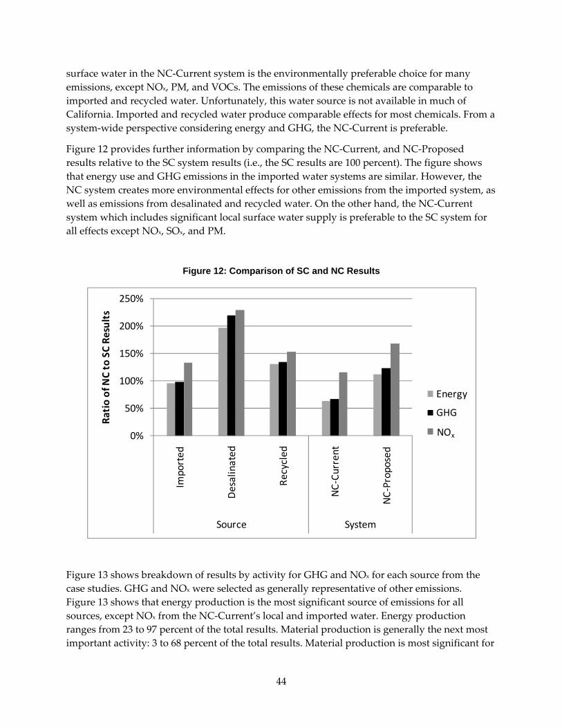
44

surface water in the NC‐Current system is the environmentally preferable choice for many emissions, except NOx, PM, and VOCs. The emissions of these chemicals are comparable to imported and recycled water. Unfortunately, this water source is not available in much of California. Imported and recycled water produce comparable effects for most chemicals. From a system‐wide perspective considering energy and GHG, the NC‐Current is preferable.

Figure 12 provides further information by comparing the NC‐Current, and NC‐Proposed results relative to the SC system results (i.e., the SC results are 100 percent). The figure shows that energy use and GHG emissions in the imported water systems are similar. However, the NC system creates more environmental effects for other emissions from the imported system, as well as emissions from desalinated and recycled water. On the other hand, the NC‐Current system which includes significant local surface water supply is preferable to the SC system for all effects except NOx, SOx, and PM.

Figure 12: Comparison of SC and NC Results

Figure 13 shows breakdown of results by activity for GHG and NOx for each source from the case studies. GHG and NOx were selected as generally representative of other emissions. Figure 13 shows that energy production is the most significant source of emissions for all sources, except NOx from the NC‐Current’s local and imported water. Energy production ranges from 23 to 97 percent of the total results. Material production is generally the next most important activity: 3 to 68 percent of the total results. Material production is most significant for

0%

50%

100%

150%

200%

250%

Imported

Desalinated

Recycled

NC‐Cu

rrent

NC‐Proposed

Source System

Ratio of NC to SC Re

sults

Energy

GHG

NOXNOx

45

NOx emissions from the NC‐Current’s local surface water source (68 percent) and the imported water system (48 percent) because of the amount of infrastructure required to supply water. Energy production for the imported water system is a similar 47 percent. Material delivery, equipment use, and sludge disposal are less than 7 percent of the total results for all scenarios.

Figure 13: Activity Contribution to GHG and NOx Results

Figure 14 illustrates the contribution of life‐cycle phases (construction, operation, maintenance, and end‐of‐life [EOL]). Figure 15 shows the contribution of water supply phases (supply, treatment, and distribution) to the overall system results (i.e., per 100 AF of water provided by the utility). The results for each source are proportioned according to the contribution to the overall supply.

For life‐cycle phases, operation dominates the results primarily because day‐to‐day electricity and chemical use occurs during this phase. Maintenance is also significant for the NC‐Current system because their distribution system is extensive and complex. End of life is least significant; for all but the NC‐Current system, the EOL contribution is less than 0.5 percent of the results for all chemicals.

0%10%20%30%40%50%60%70%80%90%100%

Imp Desal Rec Imp Desal Rec Local Imp Desal Rec Imp Desal Rec Local

SC NC SC NC

GHG NOx

Material Production Delivery / Transport Equipment Use

Energy Production Sludge Disposal

NOx

Imp= ImportedDesal = DesalinatedRec = Recycled

46

Figure 14: Life-cycle Phase Results for Utilities

Figure 15: Water Supply Phase Results for Utilities

0%10%20%30%40%50%60%70%80%90%

100%

SC

NC‐Cu

rren

t

NC‐Prop

osed SC

NC‐Cu

rren

t

NC‐Prop

osed

GHG NOx

Contribu

tion of Life

cycle Ph

ases

End‐of‐Life

Maintenance

Operation

Construction

NOx

0%10%20%30%40%50%60%70%80%90%

100%

SC

NC‐Cu

rren

t

NC‐Prop

osed SC

NC‐Cu

rren

t

NC‐Prop

osed

GHG NOx

Contribu

tion of W

ater Sup

ply Ph

ases

Distribution

Treatment

Supply

NOx

47

Supply is the most significant water supply phase for SC. The result reflects the large contribution of imported water. For the NC‐Current system, distribution is most important because of its complexity. The topography of the service area is hilly so the communities served are spread out and water must be pumped between elevations. However, for the NC‐Proposed system, treatment is also a significant contributor to the overall results, comparable to the distribution system, because of the energy‐intensive desalination process.

Since WEST was created in 2004, many changes have been made to the tool. The results of this study were different from those reported in (Horvath 2005) for some chemicals and environmental effects. In addition, due to additional changes made to the tool and to case study assumptions through the course of the project, the results in this chapter are different from the final case study results reported in Chapter 12.

A summary of the changes to WEST which have affected the final results follows:

1. The revision to the allocation of materials to the construction and maintenance phases generally reduced the contribution of material production to the results. The original calculation double‐counted some purchases. The revised calculation assigns the first purchase to the construction phase and all future costs to the maintenance phase, eliminating double‐counting. The change reduces the number of purchases, affecting material delivery and fuel production. The results changed most for sources with significant maintenance requirements (e.g., the NC‐Proposed’s desalination system).

2. The inclusion of the life‐cycle effects of electricity production significantly changes results for SOx, NOx, VOCs, and CO. For these chemicals, the “upstream” contributions to natural gas generation, California’s largest source of electricity, are more than four times the direct emissions. For PM, the “upstream” contributions are approximately equivalent to the direct emissions.

3. The update to Year 2004 eGRID data affected the following EFs for California: NOx decreased 40 percent, SOx decreased 25 percent, and GHGs increased 11 percent.

In addition, EFs for VOCs and PM in California’s electricity production were assumed to be zero before the life‐cycle effects were incorporated. Now these values are available in the tool.

The explanations listed above will be referred to be number in the discussion that follows. Overall, the original results for energy, GHG, and NOx changed the least. Generally the new results for these chemicals were higher as a result of (1). For NOx emissions due to desalination and for the NC’s recycled water systems, the new emissions decreased. These systems require significant maintenance and were affected by (1). Because of (2), one might expect that NOx emissions would have increased more dramatically. However, the reduction in the overall EF (3) limited the growth of NOx emissions.

The new results for SOx, VOCs, PM, and CO were significantly higher than the previously reported values, in some cases increasing by a factor of more than six. The primary reason for the increased emissions is (2). The emissions associated with processes that require significant maintenance increase the least due to (1). The emissions for PM did not increase as much on

48

average as for the other chemicals because the PM EF for the California electricity mix is exceptionally low (0.08 g/kWh). The national average for PM is 1.72 g/kWh.

5.3 Task 5 Conclusions and Recommendations The revisions completed for Task 5 make important improvements to WEST. The revised EFs for electricity capture a more complete picture of the environmental effects, including energy use and GHG emissions. The energy use factor for lifecycle effects is twice the direct energy use factor. The GHG lifecycle EF for the average California mix is approximately 50 percent larger than the direct EF. Without including these lifecycle emissions, the effects of water provision would be significantly underestimated.

The addition of the sludge disposal activity is also important. Though the effects of sludge disposal are generally small compared to the overall results, in most cases less than one percent, certain disposal choices can reduce overall GHG emissions, if only by a small amount relative to the utility’s total GHG emissions. One study found that for a large utility which serves over one million people, the total difference in GHGs between sludge disposal in a landfill that uses gas for electricity and one with no gas recovery system is 300 Mg annually (Stokes and Horvath 2010), equivalent to the emissions from 60 typical cars in a year (USEPA 2000).

Utilities can carefully review disposal options if the aspire to reduce their overall GHG emissions. However, changes to sludge disposal will not be as significant as other choices, including chemical selection and electricity sources.

49

CHAPTER 6: Task 6 – Evaluate Demand Management and Conservation Measures This task was designed to quantify the effects of reducing water demand using conservation programs. Many utilities develop programs to reduce water demand rather than develop new water supply, believing conservation programs are cost‐ and environmentally‐effective measures (Gleick et al. 2003). These may include residential water‐efficient fixtures and appliances, rain collection systems, irrigation systems, and commercial and industrial conservation technologies.

Urban water use in California is increasing, in part because a growing population creates more customers but also as individual water use increases. The average per capita water use in the state was 20 percent lower in 1960 than in 2000 (Hanak 2005). Economic growth means that Californians and others live in larger houses on larger lots with more water‐using appliances, all increasing overall water use. Because water supplies statewide are limited, conservation or demand management strategies may delay, if not completely prevent, severe shortages of water or developing new, more expensive sources of water supply.

The researchers completed an assessment of available demand management (or water conservation) strategies using a life‐cycle perspective to determine the relative effects of each and, in certain cases, how they compare to non‐conserving alternatives. The goal of this research is to supplement previously conducted work about conservation potential, nationwide and in California specifically (e.g., (Mayer et al. 2000; Gleick et al. 2003; Mayer et al. 2003; Mayer et al. 2004; Aquacraft 2005). These prior studies focused on the economic motivations for conservation, emphasizing that conservation was less expensive than constructing new supply.

Task 6 furthered the analysis by translating the monetary investments in new water supply and water conserving strategies into the life‐cycle environmental impacts of producing the infrastructure and materials needed to implement them. For the conservation strategies, the environmental effects of avoided water supply or energy generation were subtracted from the material production results. Energy generation is important for strategies that also provide additional energy efficiency or that avoid energy needed for water heating. These effects were quantified for several scenarios (e.g., the air emissions associated with installing a new fixture, replacing a fixture halfway through its life, and replacing a fixture at the end of its life). Furthermore, the environmental effects were converted into monetary units and compared. This methodology results in a more complete picture of the full costs associated with water provision and with water demand management strategies.

To provide context for California’s current water use and conservation potential, general data were obtained from a Pacific Institute report assessing water end use and fixture market penetration (Gleick et al. 2003). Duplication of this analysis was beyond the scope of this task so these data have not been verified by the authors and are presented for informational purposes only. There is debate over the accuracy of these estimates (e.g., [Chestnutt and Pekelney 2004]);

50

however, they are useful indicators of the magnitude of water use for each end use. Table 20 summarizes the overall potential for water conservation according to the original report in units of million liters (Ml) per year.

Table 20: Summary of Conservation Potential

Source: Gleick et al. 2003

The researchers analyzed indoor residential options, outdoor alternatives, and commercial, institutional, and industrial (CII) demand management strategies. A discussion of the general methodology is followed by the specific analysis for each end use.

6.1 Task 6 Approach The analysis determined the life‐cycle energy and air emission impacts of water demand management programs. The analysis focused on producing appliances, fixtures, and other materials needed to conserve one kiloliter per day (kl/d; approximately 264 gallons per day [gpd]) for a period of 20 years. Twenty years was selected as the planning horizon because it is the time frame associated with the Urban Water Management Plans which utilities must publish every 5 years. Results from previous analyses of NC‐Current’s water supply system were converted to this functional unit and time horizon so the results could be compared on an equivalent basis.

The analysis used LCA. The first step in the analysis was to inventory the material and energy requirements to meet these conservation goals, i.e., the number of appliances or fixtures necessary to conserve a kl /d for a period of 20 years was determined. Next, the economic costs of these fixtures for the consumer were calculated based on the estimated purchase price. The economic savings associated with conserved water and, when applicable, energy efficiency were also included. The equations used and sample calculations are included in Appendix F.1.

EIO‐LCA EFs were used to estimate the environmental effects of manufacturing water‐conserving equipment (CMU 2005). EIO‐LCA allows the user to input a production cost for a

Residential Indoor 2,800,000 1,100,000 39% 1,100,000

Residential Outdoor1 1,800,000 580,000 32% 580,000 Commercial/ Industrial/ Institutional 3,100,000 1,200,000 39% 810,000

Unaccounted water 1,200,000 --

Total 8,900,000 2,880,000 2,490,000 Notes:1 Value reported is average of the range reported in the original source.

Sector

Estimated Year 2000 Use (Ml/yr)

Conservation Estimate (Ml/yr)

Reduction Potential

(%)

Minimum Cost Effective

Reduction (Ml/yr)

51

product or service (in $), select the appropriate economic sector, and automatically calculate economic and environmental effects throughout the product’s entire supply chain. The following effects can be calculated: energy use and GHGs, NOx, PM, SOx, VOC, and CO. Table 21 provides the relevant EIO‐LCA EFs. Equations and summary calculations used in the analysis are described in Appendix F.1.

Table 21: EIO-LCA Emission Factors by Sector

Source: Carnegie Mellon University 2007

The user enters material production costs, rather than consumer prices, into EIO‐LCA. It is difficult to determine accurate producer prices when a wide range of materials are required.

Energy GHG NOx PM SOx VOC COMJ/$ g/$ g/$ g/$ g/$ g/$ g/$

Vitreous china plumbing fixture, china & earthenware bathroom accessories manufacturing 13 890 1.5 0.24 1.5 1.0 8.6Enameled iron & metal sanitary ware manufacturing 8.5 640 1.3 0.34 1.7 0.75 5.0Iron & metal sanitary ware + semiconductors (infrared sensors; custom sector) 8.5 640 1.3 0.36 1.9 0.80 5.2

Plastics plumbing fixture manufacturing 11 810 1.8 0.28 2.0 2.0 7.2Household laundry equipment manufacturing 9.9 810 1.7 0.58 1.9 1.9 8.7

Laundry + electronics (custom sector) 10 810 1.7 0.58 1.9 1.9 8.7

Natural gas distribution 14 2200 2.5 0.23 2.3 5.3 4.3

Fertilizer, mixing only, manufacturing 37 3200 4.9 0.85 3.3 2.7 13

Greenhouse & nursery production 8.1 770 2.1 1.40 1.8 1.5 12.0

Water, sewage, & other systems 11 7800 1.1 0.13 1.3 3.8 2.2

Industrial process variable instruments 4.2 340 0.72 0.21 0.89 0.59 3.6

Plastics pipe, fittings, & profile shapes 15 1100 2.3 0.31 2.5 2.4 9.6

Sawmills 8.3 710 2.4 5.0 1.4 5.3 38

Ready-mix concrete manufacturing 22 2000 7.9 1.0 6.3 5.6 17

Iron & steel forging 13 1100 1.9 0.72 2.4 1.1 8.7

Paint & coating manufacturing 16 1200 2.0 0.74 2.2 2.9 9.9

Fabricated structural steel manufacturing 9.4 830 1.6 0.68 2.0 1.0 8.9

Steel wire drawing 14 1300 2.3 1.00 2.6 1.4 14.0Watch, clock, & other measuring & controlling device manufacturing 5.7 450 0.9 0.32 1.6 0.7 5.1

Metal valve manufacturing 6.6 530 1.1 0.37 1.6 0.7 5.1

S&, gravel, clay, & refractory mining 19 1300 1.9 0.29 2.9 0.7 3.7

Sector

52

Unless otherwise noted, producer costs are assumed to be 60 percent of the consumer price for all materials.

To allow comparison of water conservation alternatives on an economic basis, the air emissions are translated into dollars using estimates of their external costs from (Matthews and Lave 2000). Matthews conducted a literature survey to determine the range of external cost estimates for these air emissions. Table 22 provides the ranges; median values were used for the calculations. Equations and sample calculations are shown in Appendix F.1.

Table 22: External Cost Estimates

Source: Matthews and Lave 2000

The evaluation also estimates the economic and environmental effects of avoided water and energy. The economic analysis uses East Bay Municipal Utility District’s (EBMUD) water and sewer costs (1.4 cents/l or 3.66 per thousand gallons [gal.], from [Aquacraft 2005]) and Pacific Gas and Electric’s electricity and natural gas costs ($0.114/kWh and $1.3/therm, respectively, based on a 2007 residential consumer bill). These results were compared to the emissions associated with supplying water based on previously analyzed case study data.

Typical water supply costs used for comparison were obtained from (MWD 1996). Emission factors for natural gas distribution, used primarily to assess natural gas water heaters, are from EIO‐LCA (see Table 21). Energy emissions for electricity were obtained from the October 2007 version of WEST. Emissions factors for water supply are based on results from the NC‐Current case study. The water and electricity EFs were presented and discussed in Chapter 6.

Several scenarios were considered during the economic analysis, as appropriate:

• Full purchase: Evaluation uses 100 percent of the economic costs for the purchase costs and 100 percent of the associated environmental effects of production.

• Early replacement of fixture: Evaluation assumes half of the economic life remains in the fixture. Evaluation uses 50 percent of the economic costs and 50 percent of the associated environmental effects.

Minimum Median Mean MaximumGHG 2 14 13 23NOx 220 1,100 2,800 9,500 PM 950 2,800 4,300 16,000 SOx 770 1,800 2,000 4,700 VOC 160 1,400 1,600 4,400 CO 1 520 520 1,100

External Costs ($/Mg of Air Emissions)Effect

53

• Marginal costs of fixture: In some cases, an average fixture and a water‐conserving fixture which are otherwise comparable are produced by the same manufacturer (e.g., washing machine). Evaluation assumes a fixture will inevitably be purchased; therefore, the evaluation uses the difference in the economic costs of the two machines for the purchase costs and an estimate of the marginal production costs specific to the product for the associated environmental effects.

• End‐of‐life replacement of fixture: Evaluation excludes purchase costs and the associated environmental effects of production because they are considered inevitable.

Any exceptions to these scenarios are discussed below. Assumptions, equations, and calculations are summarized in Appendix F.

6.1.1 Indoor Demand Management Approach

Indoor demand management was targeted as the initial and most detailed analysis for two reasons. First, there is significant potential for consumption reduction (see Table 20). Second, the strategies for reduction are easily‐defined and fairly uniform between homes. Conversely, the other major area for water conservation potential, the CII sector, requires different strategies for each industry type and can be facility‐specific. The CII sector is therefore difficult to analyze.

Indoor water use estimates broken down by fixture are shown in Table 23. The data in this table were taken from (Gleick et al. 2003). Since they are used only for illustrative purposes, the data have not been verified by the authors. The indoor demand management assessment included toilets, showerheads, faucets, and washing machines. Leaks are another major source of household wasted water. A large portion of the leaks in homes occur at toilet flappers. Retrofitting toilets repairs these leaks and reduces overall water use. Water conserved through toilet leak repair is discussed and analyzed in the “Toilets” section.

Table 23: Summary of Indoor Water Use

Source: Gleick et al 2003

Toilets 910,000 40% 520,000 57%

Showers 610,000 27% 150,000 25%

Washing Machines 410,000 18% 140,000 34%Dishwashers 30,000 1% 16,000 53%

Leaks 350,000 15% 280,000 80%

Faucets 520,000 23% -

Total 2,800,000 123% 1,100,000 39%

Fixture

Estimated Year 2000

Use (Ml/yr)

Fraction of Indoor Use

(%)

Estimated Cost Effective

Savings (Ml/Yr)

Reduction below Current

Use (%)

54

Performance data for fixtures and appliances were obtained from a series of residential water conservation studies performed by Aquacraft, Inc., Water Engineering and Management of Boulder, Colorado (Mayer et al. 2000; Mayer et al. 2003; Mayer et al. 2004; Aquacraft 2005). These studies were completed in three utility service areas (Seattle Public Utility [SPU] in Washington; EBMUD in the vicinity of Oakland, California; and Tampa Water Department [TWD] in Florida) between 1999 and 2004. In addition to reports for these utilities individually, one final overview report was produced in 2005 for the U.S. EPA. The studies are collectively referred to as the “Aquacraft reports or studies”.

Each study included approximately 30 single family homes. Water use was analyzed for a period of approximately two weeks to provide baseline data. Then new water conserving fixtures were installed and water use was analyzed for two additional two‐week periods. Key parameters of each study are summarized in Table 24.

Table 24: Aquacraft Studies Summary

Source: (Mayer et al. 2000; Mayer et al. 2003; Mayer et al. 2004)

Table 24 illustrates some differences inherent in the three studies. Aquacraft conducted a statistical analysis on the results of the three studies and determined that differences in home size and occupancy affected total household water use in a statistically significant way. Water prices were not found to be significant to the changes in water use. However, the lower prices in EBMUD and TWD may explain in part why baseline water use in these areas was higher.

Some difference in “fixture” performance may actually be attributed to the study location and overall water use patterns in that area. The utility where each fixture was used is listed in the table of the fixture’s performance data. However, the Aquacraft data were used regardless of these shortcomings because these data were the best available. For our analysis, the average performance data from the three studies were used unless otherwise noted. Customer satisfaction ratings for the fixtures themselves are provided (when available) to demonstrate that the performance of different models was comparable.

SPU EBMUD TWD

37 33 26

$11.27 $3.66 $5.67

1879 2054 1627

2.51 2.75 2.92

209 259 266

128 171 144

39% 34% 46%

Total Base-line Water Use (kl/yr)

Total Post-Retrofit Water Use (kl/yr)

Reduction (%)

Study Details

Homes studied (#)

Water prices (per thousand gal)

Average home size (square feet)

Occupancy (people/hh)

55

The following sections discuss the assumptions and data used to analyze the indoor conservation fixtures included in this study: low‐flow toilets, showerheads, faucets, and washing machines. Assumptions, equations, and calculations are summarized in Appendix F.1.

6.1.1.1 Low-Flow Toilets The Federal Energy Policy Act (FEPA) of 1994 mandated that all toilets purchased have a maximum flush volume of 6.1 l or 1.6 gal. Toilets with higher rated flush volumes are no longer available. However, as toilets age, their performance deteriorates. As a result, low‐flow toilets may use more than their rated flow of water.

The three Aquacraft studies analyzed the performance four types of toilets listed with their rated water use: standard gravity flush (6.1 l per flush [lpf], dual flush (user selects either 3 lpf or 6.1 lpf), pressure‐assisted flush (4.2 1pf or 1.1 gpf), and a flapperless flush (6.1 lpf). A pressure assisted flush toilet was included in the Aquacraft study. They analyzed a St. Thomas Creations toilet that used a Sloan Flushmate 1.1 insert. However because only two models were used, performance data were not reported. Information on the model used in the original study could not be found. Instead, a Kohler Wellworth, also with a Sloan Flushmate 1.1 insert, was analyzed. The performance and price data are based on manufacturer’s information rather than results reported by Aquacraft . Table 25 summarizes the relevant data for all toilet models.

Table 25: Toilet Performance Data

Gravity flush Dual flushPressure-

assist flushFlapperless

flush

Toto DrakeCaroma

Caravelle 305

Kohler Wellworth

Pressure Lite1

Niagara Ultimate

6.1 3.0/6.1 4.2 6.15.8 4.9 4.2 6.16.7 7.6 7.4 7.2

22385 33367 57305 54119657 3371 5255 0

13 8 5.1 5.5280$ 350$ 440$ 165$

SPU, EBMUD SPU, EBMUD EBMUD EBMUD, TWD4.67 4.31 -- 4.67

3 3.5 -- 2.3

Utility where StudiedConsumer Satisfaction Rating6

Payback period2,7

Actual Water Use (lpf)2

Flush frequency (f/toilet/d)3

Water saved (l/toilet/yr) vs. Water saved (l/toilet/yr) Toilets Needed5

Purchase Price2

Parameters

Sample Model

Rated Water Use (lpf)

Notes:1 The EBMUD study considered a Sloan Flushmate insert into a toilet by St. Thomas Creations, rather

than Kohler., but the efficient flushing mechanism is identical. Flush volume is based on manufacturer estimate rather than Aquacraft study results. Purchase price from internet search.

2 Calculated or reported by Aquacraft (Aquacraft 2005), except as noted elsewhere.3 Calculated by the authors based on reported Aquacraft data4 Water saved reported by Aquacraft includes water saved due to leak repair during installation.5 Number of toilets needed to conserve 1000 l/d above baseline over a 20 year period.6 Consumers rated the equipment on a scale of 1 (poor) to 5 (good).7 Payback period is calculated for net replacement, using 50% of purchase price.

56

The analysis assumed that each home had two toilets with a service life is 25 years. The number of toilets per household was not explicitly provided in the Aquacraft studies but the two‐toilet assumption is consistent with their data. A literature review indicates toilet service life estimates range from 20 to 40 years. The 25 year assumption is conservative.

Much of the water used in toilets is lost by leaks, especially at the toilet flapper. In the Aquacraft study, their estimates of household water conservation included savings for toilet flushing and leak repair. The analysis includes the benefit of repairing leaks. As a result, the conserving nature of these toilets may be over‐stated on an individual basis (i.e., a home without a leak will not conserve the estimated water volume) but is indicative of the conservation on a larger scale.

The EIO‐LCA sector “Vitreous China Plumbing Fixture and China and Earthenware Bathroom Accessories Manufacturing” was used to determine emissions associated with toilet production.. Ceramic parts were assumed to be the major contributors to the results and to be comparable for all models. Because toilets use only cold water, there is no energy savings associated with more efficient toilets.

6.1.1.2 Showerheads FEPA mandates that showerheads must have a flow rate less than 9.5 liters per minute (lpm, 2.5 gal. per minute [gpm]). The Aquacraft baseline study indicated water use is already below the mandated flow rate even when conserving showerheads are not used. For the three studies, the baseline flow rate ranged from 7.6 to 8.5 lpm, indicating the average users do not use the full flow range. Four models of low‐flow showerheads were analyzed by Aquacraft. Two models were standard 9.5 lpm models, one was a 6.6 lpm model, and the last was a hand‐held model with a 8.9 lpm flow rate. Detailed data used in the analysis are provided in Table 26.

Table 26: Showerhead Performance Data

ParametersBrasscraft

LFAM Conservation

SpoilerNiagara

Earth1Niagara Earth

Handheld1

Rated flow (lpm) 9.5 9.5 6.6 8.9Actual flow (lpm)2 7.1 6.9 6.2 8.3Shower use (min/day)4 5.0 7.3 10.4 10.4

Water saved (l/yr) vs. baseline2 1,382 2,082 6,596 678 Water saved (l/yr) vs. 9.5 lpm standard3 4,400 7,100 12,000 4,400

Shower-heads needed4 423 281 105 109Purchase Price5 $18 $14 $17 $30Utility where studied SPU EBMUD TWD TWDConsumer satisfaction rating6 4.58 4.43 4.44 4.44Payback period7 1.5 3.1 0.75 0.75Notes:

2 Calculated or reported by Aquacraft (Aquacraft 2005)3 Calculated by the authors based on reported Aquacraft data4 Number of showerheads needed to conserve 1000 l/d above baseline over a 20 year period.5 Purchase prices based on internet search.6 Consumers rated the equipment on a scale of 1 (poor) to 5 (good).7 Payback period is calculated for net replacement, using 50% of purchase price.

1 Water use for Niagara showerheads were reported together and disaggregated by the authors as described in Appendix F. Satisfaction ratings for Niagara showerheads were not disaggregated.

57

Each home was assumed to have two showerheads. The service life of each showerhead was assumed to be 12.5 years based on the Aquacraft studies. Aquacraft reported the performance for the two Niagara showerheads in aggregate. The authors disaggregated the data based on the expected flow rate using calculations described in Appendix F.1. The showerheads studied were primarily plastic construction; the EIO‐LCA sector “Plastics Plumbing Fixture Manufacturing” was used in the analysis.

Surprisingly, Aquacraft indicated the reduced flow did not reduce overall hot water use in an statistically significant way. As a result, no energy savings were calculated for showerheads.

6.1.1.3 Faucets Two types of conservation measures were used for faucets: aerators and hands‐free devices. Faucet aerators are installed on existing fixtures to restrict flow. The two hands‐free devices functioned differently. The first device was a faucet controller which required the user to lean on a pushbar or step on a pedal to activate the faucet; this device is used in addition to the existing faucet and, if applicable, aerator. The Aquacraft studies analyzed the Aqualean™ device (pushbar mechanism); however, the authors could not find price data for this device. Instead, price data is for a Pedalworks™ foot‐activated device. Performance for both devices is expected to be similar. The second device (Delta e‐flow) is a faucet with infrared sensors to activate the faucet. Both mechanisms prevent water from running continuously when not needed. Table 27 includes the relevant information for analyzing the faucet systems.

Table 27: Faucet Performance Data

ParameterRated Water Use (lpm)3

Actual flow (lpm)4

Faucet use (min/d)5

Water saved (l/yr) vs. baseline4

Household Sets of Faucets N d d6Puchase Price7

Energy saved vs. baseline (kWh/yr)/(therm/yr)8 55 / 35 83 / 140 11 / 18 75 / 130

Utility where Studied9

Satisfaction Rating10

Payback period4,11

Notes:

9 EBMUD study results were not included because faucet use did not cause a statistically significant reduction in water use.10 Consumers rated the equipment on a scale of 1 (poor) to 5 (good). It the appliance was used by multiple utilities, average ratings are listed.11 Payback period is calculated for net replacement, using 50% of purchase price.

1 No information was found about the Aqua-lean hands-free faucet controller from an internet search. Price is for a PedalWorks™ hands-free faucet control. Performance of these devices is assumed to be similar. Aqua-lean performance indicated the device conserved an additional 0.5 gal/person/day; the marginal savings is the only water included in the analysis.2 The purchase price listed reflects the total purchase price ($317) minus the cost of a comparable, non-hands-free Delta model ($119), as reported by Aquacraft.3 Abbreviations: (k) = kitchen, (b) = bathroom4 Calculated or reported by Aquacraft (Aquacraft 2005)5 Calculated by the authors based on reported Aquacraft data6 Number of devices needed to conserve 1000 l/d above baseline over a 20 year period.7 Purchase prices based on internet search and is the lowest cost for bulk purchases, when available.8 Calculations and assumptions for hot water calculations are described in Appendix F.1.

4.39 4.3 4.7 3.79

2 0.77 -- 12.4

$3 $6 $290 $317

Seattle Tampa Tampa Tampa

4,160 13,749 2,017 11,368

88 27 181 32

3.7 2.8 -- 2.7

29 28 -- 33

Hands-free faucet controller1

Delta e-Flow hands-free faucet2

8.3 (k), 5.7 (b) 5.7 (k), 3.8 (b) -- --

New Resources Group Niagara

58

All faucet control devices were analyzed using the EIO‐LCA sector is “Enameled Iron and Metal Sanitary Ware Manufacturing.” Aquacraft reported most homes had one kitchen faucet and two bathroom faucets. In most cases, aerators installed in the kitchen allowed a higher flow rate than aerators installed in the bathroom. However, the flow trace software used by Aquacraft to complete their water use assessments could not distinguish between water used in the kitchen and in the bathroom. Therefore, the results could not be disaggregated and faucets were analyzed on a household basis rather than for each individual fixture.

For the two hands‐free devices, the standard assumption that producer price is equivalent to 60 percent of consumer price was not appropriate. The hands‐free pedal or push bar is a device made of standard plumbing equipment. The simplicity of the fixture indicates the $290 price tag reflects a significant markup over the producer costs. The producer price was assumed to be 10 percent of the consumer price in the EIO‐LCA analysis for this fixture.

Similarly, the Delta eFlow device cost $319 while a comparable Delta faucet cost $119. The infrared sensor added to the faucet does not account for the $200 markup. In the EIO‐LCA analysis for this product, the lower price of $119 was used in the assessment; 10 percent of the semiconductor sector EF (g/$) was added to the standard EF for metal sanitary ware to account for the added infrared sensor, effectively assigning the sensor a cost of $11 per unit. Aquacraft did not report an overall household savings for the Aqua‐lean faucet controller. They reported the devices saved an additional 1.9 l/d (0.5 gpd) per person, however only two fixtures were installed so the results were less robust.

The overall water flow reduction also reduced hot water use and, therefore, energy use. Hot water use was analyzed specifically in Aquacraft’s SPU and EBMUD studies, but not in the TWD study. The estimates of hot water consumption in SPU and EBMUD were used to allocate the reduction in hot water use for the TWD study. The calculations used the water and energy costs for the EBMUD (California) service area. It was assumed that 80 percent of hot water heaters use natural gas (65 percent efficient) and 20 percent use electricity (93 percent efficient). Because electricity costs are higher than natural gas, these assumptions are fairly conservative.

6.1.1.4 Clothes Washing Machines Clothes washing machines are not subject to federal regulation. Consumers can freely choose more or less efficient machines. Washing machines on today’s market vary widely in their water consumption, from less than 75.7 l/load to more than 170 l/load (20 gal./load to >45 gal./load) based on an internet search. In addition, water‐conserving machines reduce hot water use, resulting in additional energy savings. Some machines may be more energy efficient. Many consumers do not purchase water‐conserving machines because the first costs are higher than a comparable non‐conserving machine, even though life‐cycle costs can be lower. Six washing machines models were examined in the Aquacraft reports. Some models were top‐load (or vertical axis) machines, while others were front‐load (horizontal axis machines). Table 28 includes the assumptions associated with washing machines included in this analysis.

59

Table 28: Washing Machine Performance Data

Water conserving machines are marketed as “green”, resulting in a price markup. Some of these machines do contain more sophisticated electronics than a comparable non‐conserving machine. For washing machines, a part of the “Household Laundry Equipment Manufacturing” EIO‐LCA sector, it was assumed that the cost of production was similar to the purchase price of a non‐conserving comparable machine. The contribution of the “electronics” sector to the overall supply chain was doubled for high‐efficiency washer, a conservative assumption. The custom EF used for washing machines is shown in Table 21.

Energy savings were calculated using the Energy Star life‐cycle costs calculator for washing machines developed by the U.S. EPA and U.S. Department of Energy (Energy Star 2007). The analysis assumed 80 percent of the machines were supplied by gas water heaters and the remaining by electric, as discussed in the “faucets” section.

6.1.2 Commercial, Industrial, and Institutional Demand Management Approach

There is great potential for conservation by non‐residential consumers, namely in the CII sectors. However, the activities of all the business and entities included under this umbrella are

ParameterActual water use (l/load)1

Washer use (load/d)1

Water saved (l/yr) vs. baseline1

Machines Needed2

Purchase Price3

Comparable Machine Cost3

Energy savings (kWh/yr) / (therm/yr)4 320 / 21 200 / 13 200 / 14 290 / 19 190 / 13 200 / 13

Utility where Studied

Type

Satisfaction Rating5

Payback period1,6

Notes:1 Calculated or reported by Aquacraft (Aquacraft 2005)2 Number of washing machines needed to conserve 1000 l/d above baseline over a 20 year period.3 Purchase prices and comparable machine costs reported by Aquacraft; when machine is used in multiple studies, the lowest cost is used.4 Results determined using a calculator on the (Energy Star 2007) website; includes energy for water heating.5 Consumers rated the equipment on a scale of 1 (poor) to 5 (good). It the appliance was used by multiple utilities, the satisfaction ratings are averaged.6 Payback period is calculated for net replacement, using 50% of purchase price.

5.9 2.5 1.0 2.9 5.7 5.5

4.81 4.38 4.81 4.65 4.84 4.83

Front load Front load Top load Top load Front load Top load

SPUSPU,

EBMUDSPU,

EBMUDEBMUD TWD TWD

$516 $207 $489 $500 $550 $450

$1,066 $682 $550 $699 $999 $899

35 26 31 35 19 24

16,000 22,400 21,300 15,800 30,300 23,500

103

1.1 0.91 0.82 0.93 1.2 1.0

Frigidaire Gallery

Whirlpool Super

Capacity+

Fisher & Paykel

EcosmartWhirlpool

DuetWhirlpool

Calypso94 88 109 111 68

Maytag Neptune

60

more diverse than the activities of a household. As a result, a comprehensive analysis of many of the conservation strategies in these sectors is beyond the scope of this task. Instead, a few representative strategies were chosen and analyzed.

To analyze the potential water savings in the CII sectors, a scenario for replacing toilets and urinals in an office building with low‐flow devices was analyzed. Outdoor conservation strategies for the CII sector are discussed with other Outdoor strategies.

To show the potential for indoor water conservation, installing waterless urinals/ultra‐low flow toilets in an office building was analyzed. This analysis evaluated a hypothetical 15‐story office building in Oakland, California. Each floor had 557 m2 (6,000 sq. feet) of office space, housed 175 employees (50 percent male/female), and had seven toilets and two urinals. Each employee was assumed to flush either a toilet or urinal three times a day (women always use a toilet; men use a toilet once and urinal twice daily) (Vickers 2001). The authors assumed employees worked 245 days a year (49 work weeks) and the number of flushes did not change with the retrofits.

The original fixtures were assumed to use water at rates typical prior to the 1994 legislation: for toilets 13.2 lpf and urinals 5.7 lpf. Based on these assumptions, the fixtures would use an average of 14,300 and 3070 kl/yr, respectively. Two water conserving toilets and two urinals were compared. The toilets used 1.6 gpf and 1 gpf; the urinals evaluated were a 1 gpf model and a waterless urinal. The waterless urinal analyzed required a trap seal liquid chemical be used every 1500 flushes for maintenance. This chemical may not be required for all models. Table 29 summarizes the models used in this study. Toilets were assumed to have a life of 25 years, urinals 20 years. The total economic cost for all fixtures includes an installation cost of $100 per fixture. Calculations and further details are available in Appendix F.2.

Table 29: Office Building Fixture Details

6.1.3 Outdoor Demand Management

Customers consume water outdoors for a variety of reasons, including irrigation, car washing, and to supply water features. Outdoor water use is estimated as just under half of indoor use for residential customers nationwide (Vickers 2001). However, water use varies depending on land use, landscape, and climate. In California, summer outdoor water use ranges from 105 liters per square meter per month (l/m2/month) in cooler, coastal areas to 220 l/m2/month in

Toilet 1 Toilet 2 Urinal 1 Urinal 2Water Use (lpf) 61 3.8 3.8 0Fixture price $165 $440 $250 $450Chemical ($/yr) -- -- -- $25Water savings (kl/yr) 65 85 34 102

Toilets Urinals

61

desert regions (Hanak and Davis 2006). The total residential outdoor water use in the United States is approximately 100 billion l/d (26 billion gpd) and will continue to increase as the population grows (Vickers 2001). In California, the population is expected to grow by more than 11 million people in 2030. Nevertheless, the outdoor residential water savings potential (32 percent) is significant (see Table 20).

One information source defined four evapotranspiration zones for the state which are used to estimate water needs in the differing climates. The four zones (coastal, inner coastal, central, and desert) are shown graphically on Figure 17. The regions are defined based on their summer water evapotranspiration characteristics for turf grasses; these characteristics are the baseline for all water requirement estimates and are referred to as “E0”. Turf grasses are a high water‐using plant. Water requirements in other seasons and for most other plants are correspondingly lower. Constants are used to estimate the annual water needs for each scenario relative to the E0 baseline. Figure 16 provides ranges for estimates of E0 for each region.

Figure 16: Evapotranspiration Superzones

Source: Hanak and Davis 2006

Consumers and water agencies can choose from demand management strategies to minimize or control outdoor water use. However, most strategies involve some material and energy inputs and also offset water supply and sometimes energy production, all of which have energy and environmental effects. LCA is used to compare these alternatives based on a functional unit of one kl/d over a period of 20 years, similar to the assessment for indoor demand management.

62

Outdoor demand management strategies evaluated include: turf maintenance, drip irrigation, on‐site smart controllers, xeriscaping, dormant turf, rain runoff catchment, graywater systems, and water pricing options. Each alternative was evaluated for the following seven scenarios:

• An average‐sized single‐family home and lot in the coastal region (SF1);

• An average‐sized single‐family home and lot in the inner coastal region (SF2);

• An average sized single‐family home and lot in the desert region (SF3);

• A single‐family home on a large lot (“ranchette”) in the central region (SF4);

• A hypothetical multi‐family unit in the coastal region (MF);

• A commercial facility similar to a big box store in the desert region (COM); and

• A 40,000 m2 (10‐acre) industrial site in the central region (IND).

Five residential scenarios were evaluated in this assessment. For each home, only a portion of the yard was assumed to be irrigated. The remainder was assumed to be covered with impermeable materials (driveways, sidewalks, patios) or left dormant. In addition, a percentage of the irrigated area was assumed to be turf (or grass) while the remainder was assumed to be other landscaping (e.g., trees, shrubs, and flowers). The baseline analysis assumes that the non‐turf plants are divided evenly between low, medium, and high water using‐plants. The residential scenarios are discussed further below; additional scenarios for commercial and industrial outdoor water use were also analyzed and are discussed in later sections.

Average‐sized single family homes were assumed to irrigate 35 percent of their yard (Hanak and Davis 2006). These three scenarios were assumed to be located in the coastal region (San Franscisco, California), the inner coastal region (Pasadena, California), and the desert region (Palm Springs, California). A larger single‐family home on a large lot, referred to as a “ranchette,” assumed to be located near Fresno was analyzed for comparison. It was assumed that for a yard of this size only 10 percent is irrigated.

Another scenario analyzed a multi‐family 20‐unit building located in urban Los Angeles. The South Coast has the highest percentage of multi‐family units in California (39.3 percent) (Hanak and Davis 2006). The multi‐family home is assumed to irrigate 25 percent of the yard. The commercial scenario, modeling a large “big box” store assumed 3 percent of the yard area was irrigated; the industrial scenario, a manufacturing facility with landscaping, assumed 5 percent of the yard was irrigated. The data used in each scenario is described in Table 30. Detailed assumptions and calculations are described in Appendix F.3.

The outdoor water saving alternatives evaluated included: turf maintenance, drip irrigation, on‐site smart controllers, xeriscaping, dormant turf, rain runoff catchment, graywater reuse, and water pricing. The water savings is based on the results of the baseline analysis for that scenario.

63

Table 30: Outdoor Water Use Scenarios

6.1.3.1 Turf Maintenance This scenario assumes that compost is applied to turf annually. Every ten years, a significant application is completed, where approximately four centimeters (cm, 1.5 in.) of compost is mixed with the topsoil to improve the health and drainage of the soil. In the intervening years, a layer of compost of 0.6 cm (0.25 in.) is applied. For non‐turf landscaping, a layer of 5 cm (2 in.) of mulch is applied around the plant bases every two years. Compost materials are assumed to cost $30/m3; mulch, $8/m3. Compost and mulch are part of the EIO‐LCA sector “Fertilizer, mixing only, manufacturing”. This turf maintenance strategy is expected to reduce outdoor water use by 10 percent (Gleick et al. 2003).

6.1.3.2 Drip Irrigation The drip irrigation system scenario assumes that non‐turf landscaping is irrigated using the more efficient drip configuration. This method directs water near the base and roots of the plants and prevents unnecessary runoff or evaporation. Drip irrigation systems cost $0.10/m2

(Means 2004). Based on the cost guide, 85 percent of the cost was for tubing (“plastic pipe, fittings, and profile shapes” sector), 3 percent for screens (“steel wire drawing” sector), 5 percent for timers and controls (“watch, clock, and other measuring and controlling device manufacturing” sector). The remainder was for valves (“metal valve manufacturing” sector). Drip irrigation reduces water use for non‐turf landscaping by 50 percent (Gleick et al. 2003). Drip irrigation is not an effective means of watering turf. The 50 percent reduction corresponds to an overall outdoor water use reduction of 3 – 19 percent, depending on the scenario.

6.1.3.3 On-site Smart Controllers This scenario assumes on‐site smart controllers (e.g., moisture sensor probes) determine when water is needed and are used to control the irrigation system. The term “on‐site” distinguishes

Scenarios Region

Lot Size (m2)

Irrigated Area (m2)

Turf (% of

irrgated area)

Summer Water Use

(l/m2/ month)

Annual Needs

(l/m2/yr)

Baseline water use

(kl/yr) Source

Single-family1 (SF1)

Coastal 725 363 70% 110 748 208 (Hanek 2006),

AverageSingle-family2 (SF2)

Inner Coastal

836 465 75% 163 1,108 402 (Hanek 2006),


Desert 1,022 598 80% 212 1,441 686 (Hanek 2006),


Central 16,495 14,637 90% 183 1,247 3,122 (Hanek 2006),

LargeMulti-family (MF)

Coastal 879 188 50% 116 790 64 Assumed

Commercial (COM)

Desert 90,968 2,729 50% 212 1,441 5,111 Assumed

Industrial (IND) Central 40,467 40,467 60% 183 1,247 1,715 Assumed

Residential

64

these systems from the more expensive satellite‐controlled systems. These systems prevent irrigation when there has been recent rainfall, preventing over‐watering or runoff, but are expensive and complex. Installing moisture sensors is expected to reduce overall outdoor water use by 20 percent (Gleick et al. 2003). It is assumed that the moisture systems will be used in conjunction with an existing sprinkler system if implemented. Each sensor costs $290 and is assumed to be a part of the “Watch, clock and other measuring and controlling device manufacturing” EIO‐LCA sector. Four sensors were installed at the average single family home, seven at the “ranchette”, and five at the multi‐family building.

6.1.3.4 Rain Catchment Rain catchment involves installing water storage systems, connecting them to a structure’s gutters, and collecting the runoff from the roof for future use in irrigation. This strategy is arguably more appropriate in climates where rainfall occurs throughout the year than in California’s climate where rainy and dry seasons exist. The storage capacity needed to store sufficient runoff in the winter for use three or more months later when the rain stops is more than the average residence reasonably can install due to space and cost limitations. However, these systems can still reduce overall water use, depending on the investment in storage. For residences, it was assumed that homeowners purchased a plastic container which stores 7,600 l (2,000 gal.). Each barrel is placed at gutter downspout locations and collects water until full, then redirects water away from the building. The cost of these containers is assumed to be $950 and the associated EIO‐LCA sector is “Plastics plumbing fixtures and all other plastic products.”

For CII scenarios, rain catchment for large facilities was assumed to occur in underground cisterns constructed of reinforced concrete. The cost of these cisterns is $0.09/l. The commercial facility used a cistern of 45,000 l (12,000 gal.) the industrial cistern held 34,000 l (9,000 gal.). The cisterns consist of the following materials, listed with their percentage contribution to the overall cost and the associated EIO‐LCA sector: lumber primarily for forms (10 percent, “Sawmills”), concrete (60 percent, “Ready‐mix concrete manufacturing”), reinforcing bar/mesh and lids/hatches (15 percent, “Fabricated structural metal manufacturing”), latex seal (5 percent, “Paint and coating manufacturing”), and pipes and accessories (10 percent, “Plastic pipe, fittings, and profile shapes”). The environmental costs associated with constructing the cisterns (e.g., emissions from construction equipment) were not included in the assessment. It is assumed that no new plantings or irrigation systems will be installed.

To evaluate the savings associated with rain catchment, rainfall data was used to calculate the water needed seasonally to irrigate the landscape. When rainfall exceeds need, two maximum storage volumes are assumed to be used during that period or stored for the future. Water savings associated with runoff collection ranges from 1 – 20 percent for residences. The savings for the commercial and industrial scenarios were 80 percent and 45 percent, respectively.

6.1.3.5 Graywater Systems The graywater system assumes that non‐potable piping is installed in each home or facility to collect water from sinks, showers, and washing machines for irrigation with little to no treatment. Greywater production is estimated to be 95 l/d (25 gpd) per person. It was assumed

65

that production at the commercial facility was 0.4 l per customer. At the industrial facility, the 30 l/d estimate assumes there is some process water available for use. It was assumed that 80 percent of greywater production would be captured for reuse. Assumptions for savings from graywater were limited by irrigation needs not met by rainfall. Since greywater storage is not recommended for health reasons, only 1,000 l of graywater were assumed to be needed at single‐family residences during seasons when rainfall exceeded landscaping needs. For other facilities, the volume was doubled. It was assumed that this water was used between rain events. Piping costs (interior and exterior) for the non‐potable water system were scaled based on the size of the facility. Graywater systems consisted of plastic barrels and piping (“Plastics plumbing fixtures and all other plastic products”), filters (“Sand and gravel”), and valves (“Metal valve manufacturing”).

6.1.3.6 Xeriscaping This scenario involves reducing the overall percentage of turf to 30 percent of the landscaped area for all scenarios and replacing all non‐turf landscaping with drought‐resistant, low‐water plants. The water required by the remaining turf is unchanged. The landscaping materials costs were assumed to be $27/m2 for turf and $22/m2 for non‐turf plants. The EIO‐LCA sector is “Greenhouse and nursery products.” Xeriscaping is assumed to reduce water use by approximately 40 percent, a conservative assumption based on calculations (Gleick et al. 2003).

6.1.3.7 Water Pricing Options This scenario analyzes the potential for reducing water use by changing the pricing of water by the utility. The analysis assumes outdoor water use will fall by 4 percent (Renwick and Archibald 1998). This reduction corresponds to a 10 percent price increase. Consumers are assumed to achieve the water reduction without additional investment in new plantings or irrigation systems, but only by minimizing over‐watering. There are, therefore, no economic or external environmental costs associated with this scenario.

6.1.3.8 Dormant Turf This scenario could also be called the “do nothing” scenario, literally. A minimal amount of outdoor water is used to maintain non‐turf landscaping without any change in the landscape design. There are no economic costs or external environmental costs associated with this scenario. Water use is assumed to fall by 90 percent.

6.2 Task 6 Outcomes The outcomes for demand management programs are described in this section.

6.2.1 Indoor Demand Management Results

Results are provided in terms of mass (kg) for air emissions and energy (MJ), as well as in economic terms ($). Table 31 presents the results for the NC‐Current and NC‐Proposed water supply. These results were determined as part of Task 5 but are presented for comparison to the conservation strategies. External costs were calculated by multiplying air emissions by cost estimates found in Table 22. Table 32 provides results for manufacturing water conserving

66

fixtures needed to conserve one kl /d over 20 years. For water supply, it includes all infrastructure construction and energy use for the same volume of water and time frame.

Table 31: NC Supply Environmental and Economic Result Summary

NC-

Cur

rent

S

yste

m

NC

Mar

gina

l S

uppl

y1

Impo

rted

Des

al-

inat

ed

Rec

ycle

d

Loca

l S

urfa

ce

Energy (MJ) 3,900 11,000 5,500 15,000 6,600 3,300

GHG (kg) 250 720 340 1,000 410 210

NOx (g) 580 920 610 1,300 550 570

PM (g) 120 210 130 300 120 110

SOx (g) 850 2,200 1,100 3,100 1,200 750

VOC (g) 180 410 210 570 250 160

CO (g) 1,000 2,300 1,300 3,300 1,300 920

Economic Cost- Purchase2 $6,400 $9,100 $7,400 $8,900 $11,000 $1,800

External Environmental Costs

$140 $340 $170 $490 $190 $120

Total Cost 3 $6,600 $9,400 $7,600 $9,400 $11,000 $1,900

Notes:

3 Numbers may not sum due to rounding

Life

cycl

e C

ost

($)

1 Marginal source is assumed to be an average of recycled and desalinated results. These combined sources are expected to supply the future needs of NC's customers. The marginal cost is assumed to be 90% of the average cost of these sources.2 System residential prices from (Renwick 2000); source-specific prices from (MWD 1996).

Results per kl/d Supplied

Pro

duct

ion

Em

issi

ons

67

Table 32: Environmental Effects of Indoor Residential Material Production

In most cases, the environmental effects associated with producing the conserving fixtures are higher than the emissions associated with the current system supplying the water. The one exception is the SOx emissions associated with the Niagara Ultimate toilet. The water conserving fixtures cause up to 35 times more GHG emissions than the NC‐Current system. However, when the NC needs to provide water to meet future needs, they will not be able to get significantly more water from either importation or surface reservoirs. The marginal water source is likely a combination of recycled and/or desalinated water. The average emissions from these two sources were used to estimate the emissions for marginal water in the system. When the conserving fixtures were compared to the marginal source, the analysis indicates faucet aerators and the Niagara toilet are preferable to new supply for many chemicals. The pressure‐assisted toilet and Niagara 6.6 lpm showerhead were preferable for SOx.

However, these analyses only tell part of the story, the emissions caused by fixture manufacturing. Water conservation also has economic benefits of avoided water and energy

Energy (GJ) GHG (kg) NOx (g) PM (g) SOx (g) VOC (g) CO (g)

Toto Drake 28 2,000 3,300 530 3,300 2,200 19,000Caroma Caravelle 305 22 1,500 2,600 410 2,500 1,700 15,000Kohler Wellworth Pressure Lite 17 1,200 2,000 330 2,000 1,400 12,000Niagara Ultimate 7.0 490 830 130 820 560 4,700

Brasscraft LF 48 3,700 8,100 1,300 9,000 9,300 33,000AM Conservation Spoiler 25 1,900 4,200 670 4,600 4,800 17,000Niagara Earth 11 870 1,900 300 2,100 2,200 7,700Niagara Earth Handheld 21 1,600 3,500 550 3,900 4,000 14,000

New Resources Group 1.3 100 200 54 260 120 790Niagara 0.81 61 120 32 160 72 480

Hands-free faucet controller 44 3,400 6,600 1,780 8,800 3,900 26,000Delta e-Flow hands free 19 1,500 3,000 820 4,000 1,800 12,000

Maytag Neptune 108 8,800 18,000 6,200 20,100 20,600 94,000Frigidaire Gallery 33 2,600 5,500 1,870 6,100 6,200 28,000Whirlpool Super Capacity+ 90 7,300 15,000 5,180 16,800 17,200 79,000Fisher & Paykel Ecosmart 106 8,700 18,000 6,110 19,800 20,300 93,000Whirlpool Duet 61 5,000 10,000 3,520 11,400 11,700 53,000Whirlpool Calypso 65 5,300 11,000 3,710 12,000 12,300 56,000Note: Values shown in red italics are lower than results for NC's marginal supply.

Production Emissions per kl/day

SHOWERHEADS

FAUCETAerators

ModelTOILETS

Hands free devices

WASHING MACHINES

68

purchases, as well as the avoided environmental emissions associated with them. These economic and environmental effects should all be considered in the final analysis. To assist this, the environmental emissions are translated into economic terms using external cost estimates. Four scenarios are considered: full production, early replacement (50 percent of production costs), marginal replacement, and end‐of‐life (no production costs). The last three scenarios assume that the fixture purchase is inevitable. If true, the early replacement scenario assumes only the effects above and beyond the inevitable should be included. In early replacement, the assumption is that the original fixture has exhausted half its service life and is being replaced by a more conserving fixture. For marginal replacement, the assumption is that only the price difference between the non‐conserving and the conserving fixtures should be considered. The end‐of‐life scenario assumes that the original fixture is no longer usable and therefore no production costs should be considered as they are inevitable. The four scenarios analyzed bound the choices which a consumer may make. The results for the four scenarios in monetary units, including both economic and environmental external costs, are shown in Table 33.

The analysis shown in the table is from the consumer perspective, i.e., it represents the costs and savings to the household, as opposed to the costs and savings to the utility. The analysis does not include any rebates or other incentive programs which may lower the costs of the conservation to the consumer. Rebates or incentive programs may make more alternatives reasonable from the consumer perspective.

Table 33 shows that, when the emissions are translated to monetary costs and the economic costs for energy or water are included, the total full purchase costs are less than the marginal supply costs for all toilets, showerheads, the faucet aerators, and the Delta eFlow faucet. However, the full purchase scenario does not represent most consumer purchase decisions because it assumes that a consumer is choosing whether or not to purchase a fixture for the first time. In fact, the consumer is often replacing an existing fixture, either as an upgrade or to replace a broken fixture. The early replacement and end‐of‐life scenarios are more representative of this choice. Four of the six models of washing machines are also included under the early replacement scenario.

For washing machines and the Delta eFlow faucet, a marginal replacement scenario was also evaluated. This analysis compared the water‐conserving device to a comparable non‐conserving fixture from the same manufacturer. This scenario used the price difference between the models for the purchase costs and evaluated the external production costs based on the estimated differences in material inputs for the fixtures. Two washing machines are competitive in the marginal replacement scenario.

For the NC‐Current supply system, external costs add two to six percent to the water price to capture costs of the air emissions included in the analysis. The conservation fixtures’ external costs are one to four percent of the purchase price for the fixtures. These values capture only a portion of the external costs.

69

Table 33: Economic Impacts of Water Conservation

Purchase 3,700 2,800 2,200 910 7,600 3,900 1,800 3,300 1,800 1,100 100,000 14,000 37,000 18,000 17,000 25,000 19,000 21,000

Water1 -13 -65 -100 0 -84 -140 -240 -85 -80 -270 -39 -220 -310 -430 -410 -310 -590 -450

Energy2 -- -- -- -- -- -- -- -- -1,000 -3,800 -490 -3,400 -1,300 -810 -820 -1,100 -770 -800

Production 51 40 31 13 110 57 26 47 19 11 190 56 270 82 230 270 160 160

WaterSavings3 -10 -50 -77 0 -64 -100 -180 -65 -1.5 -5.1 -0.75 -4.2 -6.0 -8.3 -7.9 -5.9 -11 -8.7

EnergyOffset4

-- -- -- -- -- -- -- -- -38 -120 -16 -110 -71 -45 -46 -64 -43 -45

FullPurchase5 3,700 2,800 2,100 920 7,600 3,800 1,400 3,200 610 -3,100 100,000 9,900 36,000 17,000 16,000 23,000 17,000 20,000

EarlyReplacement

1,800 1,300 960 460 3,700 1,800 480 1,500 -280 -3,600 52,000 3,000 17,000 7,700 7,300 11,000 7,900 9,500

Marginal Replacement

-- -- -- -- -- -- -- -- -- -- -- 4,700 17,000 11,000 580 5,500 6,900 9,400

End-of-lifeReplacement

-22 -110 -180 0 -150 -240 -430 -150 -1,200 -4,200 -540 -3,800 -1,700 -1,300 -1,300 -1,500 -1,400 -1,300

Notes:1 Assumes water costs for EBMUD as reported in (Aquacraft 2005).2 Assumes residential consumer costs from a May 2007 Pacific Gas and Electric bill.3 Emissions are esimated based on NC's marginal supply.4 Emission factors are for the average California energy mix.5 Italics indicate results which are lower than the total costs of NC's marginal supply.

Frig

idai

re G

alle

ry

Whi

rlpo

ol S

uper

C

apac

ity+

Fish

er &

Pay

kel

Eco

smar

t

Whi

rlpo

ol D

uet

Whi

rlpo

ol

Cal

ypso

New

Res

ourc

es

Gro

up

Nia

gara

Han

ds-fr

ee fa

ucet

co

ntro

ller

Del

tae-

Flow

han

ds fr

ee

May

tag

Nep

tune

Econ

omic

C

osts

Exte

rnal

En

viro

nmen

tal

Cos

tsTo

tal C

osts

Toto

Dra

ke

FAUCET WASHING MACHINESAerators Hands-free

Koh

ler

Wel

lwor

th

Pre

ssur

e Li

te

AM

Con

serv

atio

n S

poile

r

Nia

gara

Ulti

mat

e

Bra

sscr

aft L

F

Nia

gara

Ear

th

Nia

gara

E

arth

Han

dhel

d

Lifecycle Costs ($) per kl/day Conserved/ Supplied

TOILETS SHOWERHEADS

Car

oma

Car

avel

le 3

05

70

6.2.2 Indoor CII Demand Management Results

Table 34 summarizes both the material production environmental effects and the total economic costs associated with this scenario.

Table 34: Environmental Effects and Total Economic Cost Results for Office Building

The total costs for all scenarios except Toilet 1 are higher than the costs associated with NC’s marginal water supply (~$9,000). The results indicate the costs for replacing urinals are expensive given the water savings. Even the waterless urinal has high costs relative to the water savings. The total costs are approximately $7,000 less when the trap‐seal liquid is not required. However, this amount is still not comparable to water supply. The potential water savings from toilets is much greater and more cost effective.

6.2.3 Outdoor demand management results

Table 35 presents the results for outdoor water saving strategies, including materials needed to conserve one kl/d over a period of 20 years compared to supplying water. For water supply, it includes all infrastructure construction and energy use for the same volume of water and time frame.

The results indicate that the material production external costs associated with outdoor strategies tend to exceed the external costs associated with NC’s marginal supply as shown in Table 31. The smart controller (e.g., moisture sensor probes) alternative can be beneficial for certain emissions and energy use for large land users in dry climates of the inland and desert

Toilet 1 Toilet 2 Urinal 1 Urinal 2Energy (GJ) 41 83 590 1,000 GHG (kg) 2,800 5,800 41,000 57,000 NOx (g) 4,800 9,800 70,000 430,000 PM (g) 770 1,600 11,000 370,000 SOx (g) 4,800 9,700 69,000 440,000 VOC (g) 3,200 6,600 47,000 460,000 CO (g) 27,000 56,000 390,000 590,000 Purchase / installation costs $8,500 $13,000 $110,000 $56,000

Chemical costs $2,500

Water savings offset -$350 -$350 -$350 -$350Material production (fixtures, chemicals) $75 $150 $1,100 $4,000

Water savings offset -$350 -$350 -$350 -$350$7,900 $13,000 $110,000 $62,000

Note: Numbers may not sum due to rounding

Results per kl/dToilets Urinals

Mat

eria

l Pro

duct

ion

Eco

nom

ic

cost

sE

xter

nal

cost

s

Total

71

regions. In addition, rain runoff catchment and graywater reuse for large facilities is also preferable for a few environmental indicators in dry climates (i.e., energy use and SOx).

Table 35: Environmental Impacts of Outdoor Water Conservation

Energy (GJ) GHG (kg) NOx (g) PM (g) SOx (g) VOC (g) CO (g)SF1 130 11,000 17,000 3,000 11,000 9,600 47,000 SF2 80 7,000 11,000 1,900 7,100 6,000 29,000 SF3 57 5,000 7,500 1,300 5,100 4,200 21,000 SF4 55 4,800 7,300 1,300 4,900 4,100 20,000 MF 160 14,000 22,000 3,800 15,000 12,000 60,000 COM 90 7,900 12,000 2,100 8,000 6,700 33,000 IND 120 11,000 16,000 2,800 11,000 9,100 44,000 SF1 560 42,000 87,000 12,000 94,000 90,000 370,000 SF2 380 28,000 59,000 8,200 63,000 61,000 250,000 SF3 290 22,000 45,000 6,300 49,000 47,000 190,000 SF4 340 25,000 52,000 7,300 56,000 54,000 220,000 MF 530 40,000 82,000 12,000 89,000 86,000 350,000 COM 290 22,000 45,000 6,300 49,000 47,000 190,000 IND 340 25,000 52,000 7,300 56,000 54,000 220,000 SF1 61 4,900 9,900 3,400 17,000 6,400 45,000 SF2 32 2,500 5,100 1,800 8,800 3,300 23,000 SF3 19 1,500 3,000 1,000 5,200 2,000 14,000 SF4 7 600 1,200 400 2,000 750 5,300 MF 99 7,900 16,000 5,500 28,000 10,000 73,000 COM 6 500 1,000 350 1,700 660 4,600 IND 7 600 1,200 420 2,100 780 5,500 SF1 110 8,300 18,000 2,900 20,000 21,000 73,900 SF2 160 13,000 27,000 4,400 31,000 32,000 110,000 SF3 590 46,000 100,000 16,000 110,000 110,000 410,000 SF4 66 5,700 19,000 4,200 16,000 16,000 59,000 MF 85 6,500 14,000 2,300 16,000 16,000 58,000 COM 8 700 2,400 530 2,000 2,000 7,500 IND 10 900 2,900 650 2,500 2,400 9,100 SF1 240 18,000 35,000 5,100 40,000 32,000 130,000 SF2 200 15,000 30,000 4,400 34,000 28,000 110,000 SF3 190 14,000 27,000 4,000 31,000 25,000 110,000 SF4 260 19,000 38,000 5,700 44,000 36,000 150,000 MF 480 35,000 65,000 9,800 79,000 53,000 220,000 COM 97 7,100 13,000 2,000 16,000 9,700 42,000 IND 13 900 1,800 280 2,200 1,500 6,500 SF1 80 7,600 21,000 13,000 17,000 15,000 120,000 SF2 55 5,200 14,000 9,200 12,000 10,000 80,000 SF3 43 4,100 11,000 7,200 9,400 8,100 63,000 SF4 51 4,900 13,000 8,600 11,000 9,600 75,000 MF 70 6,700 18,000 12,000 15,000 13,000 100,000 COM 38 3,700 10,000 6,500 8,400 7,200 56,000 IND 46 4,400 12,000 7,800 10,000 8,700 68,000

Scenarios

Production Emissions per kl/day

Turf

mai

nten

ance

Drip

Irrig

atio

nM

oist

ure

sens

or

prob

esR

ain

barre

l ca

tchm

ent

Gre

ywat

erX

eris

capi

ng

Note: Italics indicates results lower than NC marginal supply's energy use and air emissions.

72

Table 36 presents the results in terms of economic and external environmental costs. In contrast to the residential water fixtures discussed in the previous section, only the full purchase costs are listed. The “early replacement” and “end‐of‐life” scenarios are only relevant when an existing system is being replaced, generally not the case for the landscaping and irrigation systems included in this assessment.

All alternatives except drip irrigation are preferable to water supply under this assessment under at least two scenarios. Because drip irrigation only reduces water use in the non‐turf areas, it requires significant investment (in economic and material terms) without affecting all irrigation use. The relationship between water use and system cost is assumed to be linear. Economies‐of‐scale could make drip irrigation more beneficial for larger facilities.

Turf maintenance and xeriscaping are preferable to supply for all scenarios. The costs for turf maintenance are several thousand dollars lower than replacing all the landscaping. If the landscaping plants are assumed to last twice as long, the costs for turf maintenance and xeriscaping are similar. In addition, the authors suspect that the savings estimate for xeriscaping from (Gleick et al. 2003) is conservative. They estimate savings of 40 percent but using the assumptions associated with these scenarios the savings were calculated to be 42 to 53 percent depending on the scenario.

Generally speaking, costs for smart controllers were lower than supply costs when larger, drier yards were in the scenario. Smart controllers were not preferred for the cooler, wetter San Francisco coastal climate or for the small yard associated with the Los Angeles apartment building. Rain runoff catchment is seen to be preferred in the wetter Northern California climate and for larger buildings where roofs can collect more water (multi‐family, ranchette, commercial, and industrial buildings). Graywater is only preferred for large facilities with large production of reusable water (the COM and IND scenarios).

The results for the dormant turf and water pricing alternatives are not shown in Tables 35 and 36 because the cost savings per kl /d water savings are equal to the economic cost of the water for all scenarios (‐$7,100). However, the savings per facility varies for these alternatives. Table 36 shows the water savings for certain alternatives, including water pricing and dormant turf.

73

Table 36: Environmental Effects of Outdoor System Material Production

SF1 $5,900 -$7,100 $270 -$340 -$1,200SF2 $3,700 -$7,100 $170 -$340 -$3,600SF3 $2,600 -$7,100 $120 -$340 -$4,700SF4 $2,500 -$7,100 $120 -$340 -$4,800MF $7,500 -$7,100 $350 -$340 $440COM $4,100 -$7,100 $110 -$340 -$3,200IND $5,600 -$7,100 $150 -$340 -$1,700SF1 $64,000 -$7,100 $810 -$340 $58,000SF2 $43,000 -$7,100 $550 -$340 $36,000SF3 $33,000 -$7,100 $420 -$340 $26,000SF4 $38,000 -$7,100 $490 -$340 $32,000MF $25,000 -$7,100 $770 -$340 $18,000COM $61,000 -$7,100 $420 -$340 $54,000IND $33,000 -$7,100 $490 -$340 $26,000SF1 $18,000 -$7,100 $170 -$340 $11,000SF2 $9,300 -$7,100 $90 -$340 $2,000SF3 $5,500 -$7,100 $50 -$340 -$1,900SF4 $2,100 -$7,100 $20 -$340 -$5,300MF $29,000 -$7,100 $270 -$340 $22,000COM $1,800 -$7,100 $20 -$340 -$5,600IND $2,200 -$7,100 $20 -$340 -$5,200SF1 $17,000 -$7,100 $280 -$340 $10,000SF2 $26,000 -$7,100 $420 -$340 $19,000SF3 $94,000 -$7,100 $1,500 -$340 $88,000SF4 $4,600 -$7,100 $230 -$340 -$2,600MF $13,000 -$7,100 $220 -$340 $6,200COM $600 -$7,100 $30 -$340 -$6,800IND $700 -$7,100 $30 -$340 -$6,700SF1 $27,000 -$7,100 $550 -$340 $21,000SF2 $23,000 -$7,100 $470 -$340 $16,000SF3 $21,000 -$7,100 $430 -$340 $14,000SF4 $30,000 -$7,100 $600 -$340 $23,000MF $53,000 -$7,100 $1,000 -$340 $47,000COM $11,000 -$7,100 $200 -$340 $3,400IND $1,500 -$7,100 $30 -$340 -$5,900SF1 $17,000 -$7,100 $320 -$340 $9,400SF2 $11,000 -$7,100 $220 -$340 $4,100SF3 $8,900 -$7,100 $170 -$340 $1,600SF4 $11,000 -$7,100 $200 -$340 $3,300MF $14,000 -$7,100 $280 -$340 $7,300COM $7,900 -$7,100 $150 -$340 $700IND $9,500 -$7,100 $180 -$340 $2,300

Rai

n ba

rrel

ca

tchm

ent

Gre

ywat

erX

eris

capi

ngScenario

Note: Water source is NC's marginal supply. Italics indicates results which are lower than the cost of NC's marginal supply.

System Life-cycle Costs for kL/day over 20 yearsEconomic Costs External Environmental Costs

Full CostsPurchase Water Production Water OffsetTu

rf m

aint

enan

ceD

rip Ir

rigat

ion

Moi

stur

e se

nsor

pr

obes

74

Table 37 shows that options which do not require economic and environmental investments generally create the lowest total costs. Supplying the marginal water saved in the water pricing alternative would range from under $100 to over $5000, while for the dormant turf alternative the costs would range from approximately $1500 to $80,000. This shows that avoiding water use without technological change provides the greatest benefit. Depending on the plants used in the yard, the dormant turf option may not be aesthetically pleasing for consumers and, therefore, is less likely to be adopted.

Table 37: Household/Facility Economic Impacts of Outdoor Water Conservation

However, it should be noted that the results are sensitive to a number of factors, including yard size, irrigated area, turf area, plant types, topography (i.e., some scenarios could require

SF1 $340 -$400 $16 -$20 -$71SF2 $400 -$780 $19 -$38 -$390SF3 $490 -$1,330 $23 -$65 -$880SF4 $2,100 -$6,000 $99 -$300 -$4,100MF $130 -$120 $6 -$6 $8COM $5,800 -$9,900 $160 -$480 -$4,500IND $5,200 -$6,600 $150 -$320 -$1,600SF1 $3,700 -$1,600 $70 -$77 $2,100SF2 $4,900 -$3,000 $94 -$150 $1,800SF3 $6,500 -$5,200 $120 -$250 $1,200SF4 $35,000 -$24,000 $680 -$1,200 $11,000MF $1,000 -$490 $19 -$24 $510COM $43,000 -$39,000 $830 -$1,900 $3,700IND $35,000 -$26,000 $670 -$1,300 $8,600SF1 $0 -$160 $0 -$8 -$160SF2 $0 -$300 $0 -$15 -$320SF3 $0 -$520 $0 -$25 -$540SF4 $0 -$2,400 $0 -$120 -$2,500MF $0 -$50 $0 -$2 -$51COM $0 -$3,900 $0 -$190 -$4,000IND $0 -$2,600 $0 -$130 -$2,700SF1 $0 -$3,620 $0 -$180 -$3,800SF2 $0 -$7,000 $0 -$340 -$7,300SF3 $0 -$11,950 $0 -$580 -$12,530SF4 $0 -$54,350 $0 -$2,700 -$57,002MF $0 -$1,100 $0 -$55 -$1,200COM $0 -$88,960 $0 -$4,300 -$93,307IND $0 -$59,710 $0 -$2,900 -$62,631

Wat

er P

ricin

gD

orm

ant T

urf

Turf

mai

nten

ance

Xer

isca

ping

Household/Facility System Life-cycle Costs over 20 yearsEconomic Costs External Environmental Costs

Full CostsPurchase Water Production Water OffsetScenario

75

pumping which was not included in the analysis), building size, material and water costs, etc. These results should only be taken as guidelines and not as absolute results.

6.3 Task 6 Conclusions and Recommendations 6.3.1 Indoor Demand Management Conclusions

The indoor residential demand management analysis indicates that investing in indoor residential demand management is environmentally preferable to supplying water. The Pacific Institute study indicates there is still great potential for reducing water demand by these methods (Gleick et al. 2003). Figure 17 shows the statewide potential economic savings (including external costs) for the early replacement scenario.

Figure 17: Potential Savings Statewide of Indoor Demand Management Fixtures

The analysis uses Pacific Institute’s estimates for conservation potential of toilets, showerheads, and washing machines (Table 23) and assumes installation of the most inexpensive fixture in the early replacement scenario. The results assume there are one million households in California and that low‐flow faucets have a 50 percent market penetration. The costs of conservation are compared to the costs of NC’s marginal supply. However, for washing machines, the analysis also indicates that some models are priced too high for costs to be recouped under many purchase scenarios even when water and energy savings are considered. Manufacturers should consider these outcomes when pricing their models.

There are a number of limitations to the outcome of this study. First, the results should not be taken as representative for these models under all circumstances. The original Aquacraft studies were of a limited scope, in terms of numbers of households studied and geography. Since the

-

2,000

4,000

6,000

8,000

10,000

12,000

14,000

Toilet Showerhead Faucet Washing machine

Cal

iforn

ia S

avin

gs v

s. W

ater

Sup

ply

for E

arly

Rep

lace

men

t S

cena

rio

(mill

ion

$)

76

outcomes for each fixture are tied to the Aquacraft results, they can be taken as indicative, but not absolute, comparisons. In addition, the households chosen for the Aquacraft study had above‐average water use and, therefore, had greater potential for water savings than the average household. This factor likely overestimates the water savings from replacing indoor household fixtures in an average or below average water‐consuming home. Second, an uncertainty assessment was not conducted on the results. In reality, the economic estimates of price and external costs could cover a wide range but in this study are reduced to a single number. It is an indicative value but cannot be used as an absolute outcome.

6.3.2 Indoor CII Demand Management Conclusions

In the assumed scenario, the cost of conservation should be evaluated for the particular office building. The results shown in Table 29 are sensitive to the number of flushes per day, either on because the per capita flushes or number of employees are not accurate. The result that waterless urinals do not provide significant savings relative to existing urinals was surprising. If the waterless urinal is compared to a pre‐1994 toilet the total costs are more favorable and comparable to the Toilet 2 results but are still not competitive with the assumptions made for the NC’s marginal supply.

6.3.3 Outdoor Demand Management Conclusions

The analysis of outdoor demand management indicates that many, but not all, alternatives are beneficial when compared to supplying the marginal water source using a life‐cycle perspective. Four alternatives (turf maintenance, xeriscaping, water pricing, and dormant turf) led to lower costs to consumers under all scenarios. These alternatives should be encouraged to reduce overall water use.

The analysis included in this paper implicitly assumes that these alternatives are mutually exclusive. However, some can be used in conjunction with others. While the water savings will generally increase as different strategies are employed, the water savings associated with different alternatives should not be assumed to be strictly additive.

In addition, for some scenarios there may be economic and environmental savings associated with reduced energy or chemical use. Xeriscaped yards, for example, do not require fertilizers or mowing as much as some other landscapes do. Data was not available about the frequency of feeding and mowing. Therefore, reliable estimates of these savings were impossible. However, for a comprehensive assessment, this should be considered when comparing outdoor water alternatives

77

CHAPTER 7: Task 7 – Consider Additional Pollutants WEST and WWEST were revised to include additional pollutants in the assessment. The Phase One version of WEST assessed the emissions of greenhouse gases and the resulting GHG, NOx, SOx, PM, VOC, and CO. To improve the results, various air and water toxic releases caused by production of materials and energy were also included. These results give a more comprehensive picture of the environmental effects caused by water systems.

7.1 Task 7 Approach Task 7 consisted of collecting the EF data needed to revise the tool, updating the necessary calculations and documentation, and analyzing a hypothetical case study of the use of desalinated water in California.

7.1.1 Revisions

Both tools, WEST and WWEST, were updated to include additional pollutants to land, air, and water due to material and fuel production. The emissions to land are reported as a single volume (in kg). For air and water, emissions for specific chemicals are reported in kg. Two EF sources were used to obtain additional pollutant data, EIO‐LCA and the commercially‐available LCA software, GaBi (CMU 2007; GaBi 2003). Air and water pollutants with EFs in both EIO‐LCA and GaBi were included in the analysis. Emissions to land were only available in EIO‐LCA. Tables 38 and 39 summarize the chemical air and water pollutants, respectively. All pollutants listed can now be analyzed in both WEST and WWEST.

Because the average user may not be interested in results for all chemicals, the original results pages in WEST and WWEST were left unchanged. If a user wants more detailed emissions to air and water, they can reference two new worksheets in each tool, “Results‐ALL AIR” and “Results‐ALL WATER”. Results are presented in tabular form. All EFs can be found in the new tabs: “final water efs” and “final air efs”. The calculations are similar to those described previously for assessing material production for both tools and can be generally described by Equation 7‐1 for EIO‐LCA and Equation 7‐2 for GaBi.

Equation 7‐1: tedVolumeTreariodAnalysisPe

UnitFunctionalUnitsUnitCostEIOLCAEFMPEmission*

#***=

Equation 7-2: tedVolumeTreariodAnalysisPe

UnitFunctionalUnitsUnitWeightGabiEFMPEmission*

#***=

78

Table 38: Air Emission Factors added to WEST and WWEST

1,1,1-TRICHLOROETHANE DICHLORO-

1,1-DICHLORO- TETRAFLUOROETHANE

1-FLUOROETHANE DIOXIN AND DIOXIN-LIKE

1,2,4-TRIMETHYLBENZENE COMPOUNDS

1,2-DIBROMOETHANE ETHYLBENZENE

1-CHLORO-1,1- ETHYLENE

DIFLUOROETHANE FLUORINE

ACETALDEHYDE FORMALDEHYDE

ACROLEIN HYDROCHLORIC ACID

ACRYLONITRILE HYDROGEN CYANIDE

AMMONIA HYDROGEN FLUORIDE

ANTHRACENE LEAD

ANTIMONY LEAD COMPOUNDS

ARSENIC MANGANESE

ARSENIC COMPOUNDS MERCURY

BARIUM METHANOL

BENZENE NAPHTHALENE

BENZO(G,H,I)PERYLENE NICKEL

BERYLLIUM PHENANTHRENE

BROMINE PHENOL

CADMIUM POLYCHLORINATED BIPHENYLS

CARBON DISULFIDE POLYCYCLIC AROMATIC

CARBON TETRACHLORIDE COMPOUNDS

CHLORINE PROPYLENE

CHLORODIFLUOROMETHANE SELENIUM

CHLOROTRIFLUOROMETHANE SILVER

CHROMIUM STYRENE

CHROMIUM COMPOUNDS THALLIUM

COBALT TOLUENE

COPPER TRICHLOROFLUOROMETHANE

CUMENE VANADIUM

CYCLOHEXANE VINYL CHLORIDE

DICHLORODIFLUOROMETHANE XYLENE

DICHLOROMETHANE ZINC

AIR EMISSIONS

79

Table 39: Water Emission Factors Added to WEST and WWEST

7.1.2 Case Study

The updated WEST was used to analyze the environmental effects of using desalination to provide water to coastal California. Prior data from a seawater desalination system was entered into the revised tool and used to estimate the production of water needed to supply several of California’s largest coastal cities: San Diego, Los Angeles, and San Francisco. These results are not intended to be a realistic assessment of the future of water supply in California but may be considered a worst‐case scenario.

The total water volumes needed to supply each of these cities, along with the associated utility, are listed in Table 40. The data were obtained from utility websites. The total water volume analyzed, 1,500,000 Ml/yr, represents approximately 15 percent of California’s urban water supply in the year 2000 (DWR 2005).

1,2-DIBROMOETHANE FLUORINE

1,2-DICHLOROETHANE HYDROGEN FLUORIDE

1,2-DICHLOROPROPANE LEAD

ACRYLONITRILE MANGANESE COMPOUNDS

ALUMINUM MERCURY

AMMONIA METHANOL

ANTHRACENE NAPHTHALENE

ANTIMONY NICKEL

ARSENIC NITRATE COMPOUNDS

BARIUM PHENOL

BENZENE PHOSPHORUS

BERYLLIUM POLYCYCLIC AROMATIC

BROMINE COMPOUNDS

CADMIUM SELENIUM

CHLORINE SILVER

CHLOROMETHANE SULFURIC ACID

CHROMIUM THALLIUM

CHROMIUM COMPOUNDS TOLUENE

COBALT VANADIUM

COPPER VINYL CHLORIDE

CYANIDE COMPOUNDS XYLENE

ETHYLBENZENE ZINC

WATER EMISSIONS

80

Table 40: Water Production for Three Cities

The desalination systems used to supply the water are assumed to take water from the Pacific Ocean. The plants will be more energy and material intensive than previously‐analyzed desalination systems because the salinity in the ocean is higher than the desalination sources in other case studies, brackish groundwater and San Francisco bay water. Salinity is proportional to the need for electricity and maintenance of the treatment process. Only emissions associated with treatment are included since the supply and distribution design and operation parameters will be site‐specific for any plants which may be built in these cities. The case study will be referred to as “Desal”.

All desalination plants used to provide potable water to these cities will be similarly designed with membrane filtration pre‐treatment, RO membrane treatment, and disinfection with sodium hypochlorite. The increased salinity of this system will increase the electricity use by a factor of 65 percent over a brackish groundwater system in the SC case study. Details of chemical and electricity consumption for the Desal case study are shown in Table 41.

Table 41: Ocean Desalination Case Study Details

City UtilityAnnual Potable Water Production (Ml)

San DiegoSan Diego Water Department 300,000

Los Angeles Los Angeles Department of Water and Power 830,000

San FranciscoSan Francisco Public Utility Commission 410,000

1,540,000 TOTAL

Sulfuric acid 81

Aqueous ammonia 8.4

Calcium carbonate 26

Carbon dioxide 26

Sodium hypochlorite 6.5

Other 7.5

Electricity consumption (MWh/Ml) 4.0

Chemical consumption (kg/Ml)

Note: "Other" includes chemicals with consumption <5 kg/Ml (ferric chloride, scale inhibitor, zinc orthophosphate, and fluoridation and membrane cleaning chemicals)

81

7.2 Task 7 Outcomes The revisions to WEST were tested by analyzing a hypothetical scenario for providing desalinated water to Coastal California. Table 42 shows the results for this case study per Ml and also for providing all the water to three cities: San Diego, Los Angeles, and San Francisco.

Table 42: Desalination Energy and Air Emission Results

The operational phase dominates the results for all environmental effects, primarily due to electricity consumption. Operating the system is responsible for more than 90 percent of GHG emissions. The GHG emissions associated with supplying San Diego, Los Angeles, and San Francisco, or 15 percent of the state’s urban water supply, corresponds to 3 percent of the GHG estimates for statewide energy production (CEC 2008).

Figure 18 shows the breakdown of energy, GHG, and NOx results for each activity and verifies that energy production is the most significant contributor. Material production is also important, contributing more than 10 percent to both GHG and NOx. The other activities, material delivery, equipment use, and sludge disposal, are less important (<5 percent of overall results). The emissions from sludge disposal from this plant are negative because the assumed landfill is able to capture and flare 90 percent of the methane (CH4) produced. The effect is small (‐2 percent of overall results) but is the only source of emission savings found in the analysis.

EffectResults per Ml

Results for Three Cities (x1,000,000)

Energy (GJ) 49 75 GHG (kg) 2,239 3,448 NOx (g) 1,871 2,882 PM (g) 642 989 SOx (g) 7,182 11,060 VOC (g) 1,348 2,076 CO (g) 2,365 3,642

82

Figure 18: Desalination Results by Activity

Tables 43 and 44 list the expanded emissions added as part of Task 7. Table 43 shows land and air emissions. Table 44 summarizes emissions to water. Emissions which are less than 0.1 g/Ml are not shown in either table. Expanded emissions are due solely to material production. WEST does not contain EFs for these chemicals for other activities, including energy production. The emissions associated with these other activities may be significant.

Table 43: Expanded Land and Air Emissions Results

‐20%

0%

20%

40%

60%

80%

100%

Energy GHG NOx

Sludge Disposal

Energy Production

Equipment Use

Material Delivery

Material Production

ChemicalEmission

(g/Ml) ChemicalEmission

(g/Ml)Land Releases 82 CFC-114 0.0621,1,1-Trichloroethane 0.059 Ethylbenzene 0.101,1-Dichloro-1-fluoroethane 0.10 Ethylene 1.31,2,4-Trimethylbenzene 0.013 Formaldehyde 0.211,2-Dibromoethane 0.022 Hydrochloric acid 3.41-Chloro-1,1-difluoroethane 0.048 Hydrogen cyanide 0.29Acetaldehyde 0.059 Hydrogen fluoride 0.31Acrylonitrile 0.018 Methanol 0.78Ammonia 1.8 Naphthalene 0.021Barium 0.098 Nickel 0.020Benzene 0.28 Phenol 0.032Bromine 0.027 Polycyclic aromatic compounds 0.076Carbon disulfide 0.64 Propylene 0.47Carbon tetrachloride 0.027 Styrene 0.10Chlorine 0.33 Toluene 0.36Chlorodifluoromethane 0.36 Trichlorofluoromethane 0.012Cumene 0.044 Vanadium 0.090Cyclohexane 0.16 Vinyl chloride 0.039Dichlorodifluoromethane 0.034 Xylene 0.40Dichloromethane 0.15 Zinc 0.024Note: Only chemicals with emissions > 0.01 g/Ml are shown.

83

Table 44: Water Emissions Results

7.3 Task 7 Conclusions and Recommendations 7.3.1 Revisions

The addition of land, water, and additional air emission results to WEST and WWEST will improve the functionality of the tools for users. The improvement will be most interesting to those who are interested in very specific emissions that can be important to their local environment.

A potential future improvement to the tool would be to place these results into a more meaningful context. For instance, they could be normalized by their expected toxicity or effect on water quality. Instead of seeing a chemical‐by‐chemical list, the results would be contextualized to a more meaningful outcome for users.

7.3.2 Case Study

The Desal case study provides important bounds on the results for potential desalination scenarios in California. Several urban utilities are considering or implementing desalination plants for back‐up or emergency water supply. The reliability concerns driving these decisions cannot be ignored and may necessitate the use of desalinated water. However, this analysis provides insight into the potential impact on the state’s energy supplies, also a limited resource, if this trend continues unabated.

Figure 19 compares the treatment results from the Desal case study with previously‐analyzed desalination systems. The effects of supply and distribution have not been included as they will vary depending on local conditions. The figure shows results from the SC case study (brackish groundwater) and the NC‐Proposed case study (less saline bay water) and illustrates a range of outcomes for different desalination scenarios available in the state of California. As expected, the results for seawater desalination are consistently higher than the other two designs. In the case of brackish groundwater, the difference is more than a factor of two.

ChemicalEmission

(g/Ml) ChemicalEmission

(g/Ml)Aluminum 1.6 Methanol 56Ammonia 0.25 Nickel 0.017Arsenic 0.011 Nitrate compounds 5.8Barium 0.34 Phenol 0.097Benzene 0.046 Phosphorus 0.018Chlorine 0.37 Sulfuric acid 0.54Chromium 0.029 Toluene 0.029Copper 0.027 Xylene 0.026Lead 0.019 Zinc 0.11Manganese compounds 0.091Note: Only chemicals with emissions > 0.01 g/Ml are shown.

84

Figure 19: Desalination Results Comparison

These results can better inform utilities that are comparing different potential sources of desalinated water. Further comparisons of these and other case studies can be found in Chapter 12.

0

0.5

1

1.5

2

2.5

GHG Mg

NOx kg

Emission

s per M

l

Desal

SC

NC‐Proposed

NOx

85

CHAPTER 8: Task 8 – Develop Workshops for Industry Professionals Two workshops for California water professionals were developed to introduce the capabilities of WEST to potential users. The workshops educated the industry about the issues and limitations associated with assessing the life‐cycle environmental effects of infrastructure and encouraged dialogue between researchers and practitioners in this area.

8.1 Task 8 Approach Two workshops were held, one in Northern California and one in Southern California. To minimize economic and environmental travel costs, the Northern California workshop was webcast to allow parties in other areas of the state to participate. Workshops were advertised through the California Energy Commission, the Berkeley Water Center, the Association of California Water Agencies, local American Water Works Association chapters, the California Water Environment Association, and other means.

8.2 Task 8 Outcomes The Northern California Workshop was held on December 8, 2009 on the University of California, Berkeley campus. The workshop was well attended. Forty‐three people attended in person, representing nine different utilities, five government agencies, twelve consulting firms, and six other organizations. The workshop was also webcast. At least an additional 26 people attended via the webcast (the final number was difficult to establish). Workshop feedback forms were completed by 17 of the attendees. The feedback was useful, constructive and uniformly positive, and many suggestions were incorporated into the Southern California workshop.

A second workshop was held in Southern California on February 1, 2010 at the Orange County Water District in Fountain Valley. Seventeen people attended, representing six different utilities and three consulting firms. Copies of the slides for the Northern and Southern California workshops can be found in Appendices G.1 and G.2, respectively.

Each session was scheduled for 3 hours. The Northern California session prompted many questions and ran an additional 45 minutes. The workshop presented the general LCA methodology and attendees discussed what would be considered when completing a simple LCA analysis. Participants were also introduced to the capabilities of WEST and WWEST as well as the data required for an analysis. The researchers presented results from prior case studies and discussed how these may be improved in future analyses. A question and answer period followed the formal talk. After the workshop, participants provided feedback about how they would enhance the capabilities of the tools. Participants will be invited to participate in future research as case study systems.

86

8.3 Task 8 Conclusions and Recommendations The workshops were well‐attended and demonstrate that the water and wastewater industry is interested in issues of sustainability, energy efficiency, and greenhouse gas emissions. These researchers, and the Energy Commission, should try to keep the participants, and other interested parties, apprised of the latest research and tools available for evaluating these issues after this contract ends.

87

CHAPTER 9: Task 9 – Improve Material Production Analysis In Task 9, the authors updated WEST to improve the analysis of material production and analyzed two case study systems using the updated tool.

9.1 Task 9 Approach 9.1.1 Revisions

After Phase One, environmental emissions from material production were estimated solely using EIO‐LCA with appropriate, but aggregated, economic sectors. In many cases, these sectors assessed emissions well (e.g., ready‐mixed concrete is produced all over the nation using similar process to produce a consistent product). However, other sectors include a variety of products which consist of different raw materials and using an array of manufacturing processes. Task 9 was intended to incorporate process‐based LCA techniques (e.g., GaBi [GaBi 2005]) to create more specific results for sectors which include diverse products. For example, process‐based LCA improves the analysis of different chemicals used in the treatment system.

Other revisions were completed on both WEST and WWEST are summarized below:

• Inserted new EFs for fuel production from Greenhouse Gases, Regulated Emissions, and Energy Use in Transportation (GREET) model (USDOE 2009);

• Edited fuel production calculations to include alternative fuels in both tools;

• Updated Material Delivery calculations to incorporate new EFs from (Facanha and Horvath 2007);

• Added passenger transit modes EFs from (Chester 2008); and

• Updated electricity EFs with 2005 state data from E‐GRID (USEPA 2007).

9.1.2 Case Studies

To demonstrate the capabilities of the revised WEST, two case studies were analyzed. The prior utilities analyzed served populations of approximately 200,000 people. The new case studies were selected such that one was significantly larger and one significantly smaller. In addition, the small case study uses a water source never previously analyzed, local groundwater.

9.1.2.1 Large Utility The authors selected a utility in Northern California (NC‐Large) which serves over one million people and supplies over 250 billion liters of water per year. The utility asked not to be specifically identified. Data were obtained through utility reports, web page, and communications with staff. The details of this case study were previously published in (Stokes and Horvath 2011) and are summarized below with some revisions.

88

Approximately 90 percent of NC‐Large’s water supply is imported through aqueducts from a surface water source located 150 kilometers (km) inland. Eight percent of the imported water (7 percent of tall water) is stored in reservoirs prior to use. The remainder of the utility’s potable supply is collected in local reservoirs. All water is treated conventionally, though the stored and reservoir water require more extensive treatment than water that is imported and used directly. Treated water is distributed within the service area. Table 45 provides case study details. Sludge disposal information was not provided by the utility; data from published case studies were scaled to analyze sludge disposal effects (Stokes and Horvath 2009). Sludge was assumed to be landfilled 50 km away. The landfill flares 85 percent of the CH4 produced.

Table 45: NC-Large Case Study Summary

Supply Treatment Distribution Supply TreatmentPipelines (km) 470 NA 6,510 NA NA

Steel/DI pipe (%) 96% NA 63% NA NAConcrete/AC pipe (%) 4% NA 28% NA NAPVC pipe (%) -- NA 8% NA NA

Pumps (#) 29 20 380 NAPump stations (#) 7 -- 130 NA --Reservoirs/tanks (#) 7 -- 170 NA --Electricity (MWh/yr)2 2,300 7,200 61,000 30,000 5,700 Natural gas (MBTU/yr)2 28,000 11,000 21,000 670 7200Chemicals (liter/yr)2

Ammonia -- 790,000 -- -- 140,000 Polymer -- 290,000 -- -- 43,000 Caustic soda -- 840,000 -- -- 450,000 Hydrofluosilicic acid -- 910,000 -- -- 120,000 Sodium hypochlorite -- 4,700,000 -- -- 1,100,000 Polyaluminum chloride -- 530,000 -- -- --Sodium bisulfite -- 200,000 -- -- --Alum -- -- -- -- 1,200,000

Fleet and equipment use3

Heavy-duty truck (miles/yr) --Light-duty truck (miles/yr) --Hybrid automobile (miles/yr) --Construction equipment (hours/yr) --

Notes: NA = Not available. DI = Ductile iron. AC = Asbestos cement.1 The majority of water (95%) in the system is imported. However, 8% of imported water (7% of total) is stored in reservoirs until needed. The stored water is analyzed using the imported supply data and the reservoir treatment data. The same distribution is used for all water sources. The effects of construction and operation are distributed proportionally between all water sources the three sources. The stored supply infrastructure is also used for reservoir water.2 Year 2008 electricity, natural gas, & chemical consumption; electricity (6,600 MWh) & natural gas (32,000 MBTU) consumed for miscellaneous activities were distributed between the supply, treatment, and distribution systems.3 Fleet data based on year 2007 use; fleet use was distributed between the supply, treatment, and distribution systems for this analysis.

IMPORTED1 RESERVOIR

460,0004,500,000

350,00015,000

89

9.1.2.2 Small Utility A second Northern California utility (NC‐Small) was also evaluated to demonstrate WEST’s usefulness for small systems. This utility serves approximately 50,000 customers and supplies almost 6.7 billion liters of water annually. The utility asked not to be specifically identified. Data were obtained through utility reports, web page, and communications with staff.

Local groundwater aquifers supply NC‐Small’s water. The supply system consists of 18 production and a similar number of monitoring wells. The water from ten of those wells, about half of the total volume, comes from a pure source and requires only disinfection. The remainder is treated at the individual eight wellheads, using coagulation, filtration, activated carbon, chemical addition to remove iron and manganese, and/or disinfection. Treated water is distributed within the service area. Table 46 provides case study details. Sludge disposal information was not provided by the utility and was not included in the analysis.

Table 46: NC-Small Case Study Summary

SUPPLYFull

TreatmentDisinfection

only DISTRIBUTIONPipelines (km) -- NA NA 260

Steel/DI pipe (%) -- NA NA 7%Concrete/AC pipe (%) -- NA NA 59%PVC/PE pipe (%) -- NA NA 34%

Production Wells (#) 18 -- -- --Pumps (#) 17 -- -- 28Pump stations (#) -- -- -- 10Reservoirs/tanks (#) -- -- -- 19Electricity (MWh/yr)1 2,500 88 -- 735Chemicals (liter/yr)1

Sodium hypochlorite -- 66,000 66,000 --Ferric chloride -- 2,700 -- --

Fleet and equipment use (miles/yr)2

Heavy-duty truck Light-duty truckHybrid vehicle Automobile

TREATMENT

Notes: NA = Not available. DI = Ductile iron. AC = Asbestos cement. PE = Polyethylene.1 Year 2009 data for electricity and chemical use. Treatment electricity was estimated based on the average increased electricity use above supply for wells with treatment given the well's depth and average flow. Electricity use for disinfection is assumed to be marginal compared to pumping of the well. An additional 114 kWh of electricity use for administrative purposes is included in the final results.2 Fleet data based on nine-months of use in 2009-2010; fleet use was distributed between the supply (25%), treatment (25%), and distribution (50%) systems for this analysis.

6,200140,000

4,3002,400

90

9.2 Task 9 Outcomes 9.2.1 Revisions

The revisions to WEST and WWEST have improved the tools in a number of ways, most notably by providing more recent and/or more applicable EFs for energy production, including electricity and fuel.

9.2.2 Case Studies

The two case studies described above were analyzed using WEST to evaluate the energy and environmental effects of their infrastructure and operations. Results are reported in terms of environmental effect per million liters (Ml).

9.2.2.1 Large Utility NC‐Large uses three water sources, all of which were analyzed as separate water sources and as a combination to represent typical water in the “system”. The results of the NC‐Large analysis for the sources and system are summarized in Table 47.

Table 47: NC-Large Results Summary for Sources and System

In contrast to results from prior case studies, imported water is preferable to other water sources, including local water. The water is imported through gravity aqueducts and little, if any, energy is used to transport it. Water stored in reservoirs requires more pumping than imported water. In addition, reservoir and stored water require more significant treatment, including increased energy and chemical consumption, than the more pristine imported water.

Figure 20 shows the breakdown of the system energy consumption results by life‐cycle phase (construction, operation, maintenance) and demonstrates that system operation contributes two‐thirds of the results. Operation consists primarily of energy and chemical consumption on a day‐to‐day basis. Construction uses one quarter of the energy. End of life, which consists solely of sludge disposal, is negligible (less than 0.1 percent).

Constituent Overallper Ml Imported Reservoir Stored System

Energy (GJ) 4.2 15 16 5.6GHGs (kg) 260 870 910 330NOx (g) 720 2200 2300 890

PM (g) 280 700 790 330SOx (g) 530 2100 2100 720

VOC (g) 2700 4300 4400 2900CO (g) 1300 2100 2400 1400

Source

91

Figure 20: NC-Large System Energy Results by Life-cycle Phase

Figure 21 summarizes the system energy results by water supply phase. The supply phase (29 percent) consists of aqueducts, reservoirs, and pump stations. The treatment phase (23 percent) includes all activities at the treatment plants, including filter replacement and chemical consumption. The distribution phase (48 percent) is composed of pipes, pumps stations, tanks, and valves needed to move treated water to customers in the service area.

Figure 21: NC-Large System Energy Results by Water Supply Phase

29%

23%

48%


48%

92

The system results consist primarily of imported water. Figure 22 shows the same breakdown for the local reservoir component of the water supply. In this case, the supply phase comprises about two‐thirds of the results.

Figure 22: NC-Large Reservoir Energy Results by Water Supply Phase

Five activities are included in WEST: material production, material delivery, equipment use, energy production, and sludge disposal. Figure 23 shows energy results by activity. The sludge disposal activity is not shown because it contributed negligibly (<0.1 percent). The most significant activity is energy production, primarily electricity use and natural gas consumption. Material production and equipment use are also important at 19 percent and 16 percent, respectively. The equipment use results are more significant than seen in prior case studies because the utility provided information on fleet vehicle use, excluded from prior studies due to lack of data.

64%

19%

17%


17%

93

Figure 23: NC-Large System Energy Results by Activity

9.2.2.2 Small Utility NC‐Small obtains all of its water from local groundwater. About half of the water must be treated to remove sediment and minerals; the remainder is more pristine and is only disinfected. The two levels of water treatment, full treatment and disinfection only, are reported separately along with the overall system results in Table 48.

Table 48: NC-Small Results Summary for Sources and System

The additional treatment needed for the less pristine water (i.e., filtration, chemical addition) does not add appreciably to the final results because most of the environmental effects are caused by pumping in the supply and distribution system.

19%

2%

16%

63%

Material Production

Material Delivery

Equipment Use

Energy Production

63%

Constituent per million liters

Treated Groundwater

Disinfected Groundwater

Overall System

Energy (GJ) 20 19 20GHGs (kg) 1400 1300 1400NOx (g) 3600 3400 3500PM (g) 880 840 860SOx (g) 2000 2000 2000VOC (g) 1700 1700 1700CO (g) 2100 1900 2000

Source

94

Figure 24 shows the breakdown of the NC‐Small energy consumption results by life‐cycle phase and demonstrates that operation contributes over 90 percent of the results. Operation consists primarily of energy and chemical consumption on a day‐to‐day basis. Construction uses eight percent of the energy. Maintenance contributes less than 1 percent. The geographically smaller scale system requires less infrastructure, and therefore less construction and maintenance, than NC‐Large.

Figure 24: NC-Small System Energy Results by Life-cycle Phase

Figure 25 summarizes the NC‐Small energy results by water supply phase. The supply phase (33 percent) consists of groundwater wells. The treatment phase (20 percent) includes activities at the treatment plants, including chemical consumption. The distribution phase (47 percent) is composed of pipes, pumps stations, tanks, and valves needed to move treated water to customers. The treatment process is less complex for NC‐Small and, therefore, the treatment contribution is lower. However, though the groundwater is local, the supply contribution is larger than NC‐Large’s predominately imported water supply. The pumping required to extract it from the aquifers is more significant than NC‐Large’s gravity‐fed aqueduct.

8%

92%

0.4%Construction Operation Maintenance

95

Figure 25: NC-Small System Energy Results by Water Supply Phase

Figure 26 shows NC‐Small’s energy results broken out by activity. The most significant activity is energy production (92 percent). The small scale system and simple treatment process results in low material production results relative to prior case studies (2 percent).

Figure 26: NC-Small System Energy Results by Activity

33%

20%

47%


47%

3%

0.2%

6%

91%

Material Production

Material Delivery

Equipment Use

Energy Production

91%

96

9.3 Task 9 Conclusions and Recommendations The revisions completed as part of Task 9 will provide tool users a more updated and user‐friendly analysis of their water and wastewater utilities.

The results of the case study analysis of a Northern California utility differ significantly from prior analyses and highlight the range of results that can be expected for water systems in the state, depending on water sources, system design, geography, and other factors. In contrast to other analyses, imported water appears to be preferable to the local reservoir water collected in the service area. The geography of the imported source allows the water to be gravity‐fed to the utility so electricity use is minimized. Furthermore, the treatment required for stored water is more significant than for water directly imported, increasing the advantage.

97

CHAPTER 10: Task 10 – Analyze the Energy Demand of Wastewater Systems Collection, treatment, and disposal of wastewater are significant sources of energy consumption and associated environmental emissions (CEC 2005). LCAs of wastewater systems have been conducted in other countries (see Chapter 1) and indicate that the treatment process is a significant contributor to overall electricity consumption, that the sludge treatment process can be a significant source of GHG emissions, that sludge disposal also contributes to total environmental emissions though in some cases it can reduce GHG emissions, and that treatment process choices can affect electricity use as well as GHG emissions.

The researchers created an MS Excel‐based decision‐support tool to assess California wastewater systems. The structure and framework of the tool is similar to WEST. The Wastewater Energy Sustainability Tool (WWEST) and an analysis of a wastewater utility are further described in the following sections. This work was also published in Stokes and Horvath (2010).

10.1 Task 10 Approach The framework of this study was to conduct an LCA of a large wastewater utility. LCA has been previously described in Chapter 1. Similarly to WEST, WWEST incorporates a form of hybrid LCA which leverages the strengths of each approach while minimizing the disadvantages. EIO‐LCA was used to estimate emissions due to manufacturing most of the materials used in the system. EIO‐LCA is not detailed enough to assess the operation phase. Operational effects (e.g., fleet vehicle emissions, electricity generation) were estimated using process‐based LCA. Process‐based LCA data were also used to obtain more accurate results for certain manufactured materials, including plastic pipe and treatment chemicals (see Chapter 9).

10.1.1 The Wastewater-Energy Sustainability Tool

WWEST employs user‐defined input data to evaluate emissions and energy use throughout the system life‐cycle, including construction, operation, maintenance, and end of life. The end‐of‐life phase includes only the environmental effects of sludge disposal. Decommissioning of the system, another consideration in most end‐of‐life analyses, is not included because sufficient data were not available. Additionally, a water system LCA found that decommissioning contributed less than 1 percent of the overall environmental burden (Friedrich 2002). The contribution for a wastewater system is expected to be similar.

The tool evaluates energy and material use for six categories of activities: material production, material delivery, equipment use, energy production, sludge disposal, and direct emissions from the treatment processes. Figure 27 shows the boundaries which define the analysis in this study as well as the components included in the Phase One work.

98

Figure 27: Research Boundaries

Material production assessment allows the user to inventory materials used in the system and evaluate the energy and environmental effects of their manufacture or provision throughout the supply chain using EIO‐LCA and GaBi. Materials include reinforced concrete, pipe, pumps, valves, electrical and control systems, and chemical storage equipment. Table 49 describes more fully the components of the wastewater system and supply chain included in the study.

The material delivery component assesses the emissions produced from and energy used to transport materials to the end‐use location by truck, train, ship, or airplane. Airplane transport might be appropriate for emergency delivery. Alternately, the airplane EFs could be used to analyze the effects of employee travel.

Equipment use assesses the emissions and fuel use from operating non‐transport equipment—especially construction equipment and maintenance vehicles. Both material delivery and equipment use were analyzed using a process‐based approach. Energy production focuses on the impact of producing electricity or fuel (e.g., diesel, gasoline, or jet fuel needed for vehicle operation) used in the system. Electricity generation was assessed using process‐based LCA; fuel production was assessed using EIO‐LCA.

NOTES:Bold outlines WEST research boundaries.Bold dashed outlines WWEST research boundaries.Section A from [Lundin 2002].Section B from [Stokes 2004]

Heat and Electricity Production

Energy Recovery

Transport

Incineration

Landfill

Agricultural Land

Fertilizer Production

Use

Transport

Heating of Tap Water

Storm water Collection

Rain water

Withdrawal

Distribution

Drinking Water Treatment

Chemical Production

Raw water

Wastewater Treatment

Chemical Production

A

Heat Pumps

TreatedWastewater

StormWater

DistributionReclamation Treatment

UseTransport

B

Sludge Treatment

Urban Water System

NOTES:Bold outlines WEST research boundaries.Bold dashed outlines WWEST research boundaries.Section A from [Lundin 2002].Section B from [Stokes 2004]

Heat and Electricity Production

Energy Recovery

Transport

Incineration

Landfill

Agricultural Land

Fertilizer Production

Use

Transport

Heating of Tap Water

Storm water Collection

Rain water

Withdrawal

Distribution

Drinking Water Treatment

Chemical Production

Raw water

Wastewater Treatment

Chemical Production

A

Heat Pumps

TreatedWastewater

StormWater

DistributionReclamation Treatment

UseTransport

B

Sludge Treatment

Urban Water System

99

Table 49: LCA System Boundaries

Each item entered in the tool must be categorized by the user according to life‐cycle phase, construction, operation, maintenance or end of life, defined as follows:

• Construction includes facility construction and production, delivery, and installation of equipment present at system start‐up, as well as construction equipment operation.

• Operation includes chemicals, non‐capital materials (i.e., cartridge and bag filters), and energy used by the system continuously.

• Maintenance includes replacement parts for capital equipment (e.g., piping, pumps, membranes, and filter media) and cleaning chemicals.

• End of life includes all activities associated with sludge disposal once it has been treated fully, mainly transport, final disposal, and electricity and/or fertilizer offsets.

In addition, each item should be defined as a component of the wastewater process: collection (transporting water through sewer lines to the treatment plant), treatment (ensuring discharged water meets regulatory standards), or discharge (transporting treated water to the discharge point). WWEST could be useful for several audiences, including planners, designers, construction contractors, plant operators, utility administrators, and policy analysts. WWEST can evaluate the environmental effects when:

• comparing distributed treatment to centralized systems when designing for expansion

• changing treatment process to reduce emissions to receiving waters or adjusting to changes in air emission standards;

Life-cycle Phase

Summary of Activities in Boundary

-Fuel use & emissions for construction equipment & delivery vehicles; -Energy use & emissions for production of construction materials, treatment equipment, & energy used in initial installation, including the supply chain.

-Energy & emissions for operating collection, treatment, & discharge phases;-Energy generation offsets from treatment operation;-Fuel use & emissions for delivery & operational vehicles; -Energy use & emissions from producing chemicals & other routinely used materials (including supply chain); -Direct emissions from the treatment process.-Energy use & emissions used to produce replacement parts for materials with service lives shorter than the analysis period (including supply chain);

-Fuel use & emissions from maintenance & delivery vehicles.-Fuel use & emissions for transporting & disposing of sludge; -Long term emissions, energy generation offsets, & fertilizer production offsets from disposal site (e.g., landfill).

Construction

Operation

Maintenance

End-of-life

100

• evaluating alternative treatment for filtration, disinfection, or natural treatment processes; and

• choosing materials for infrastructure improvements, such piping material (e.g., steel , concrete, plastic, iron).

Generally, the tool can be used to identify areas where energy efficiency improvements can be focused, material use can be reduced, and environmental burden can be minimized.

WWEST is an Excel‐based spreadsheet and contains worksheets in five categories: (1) data entry, (2) data, (3) calculations, (4) results, and (5) help. These worksheet types are discussed in the following sections. Appendix A.2 contains a copy of WEST. The WWEST user manual and revision log are in Appendix A.2.1 and A.2.2., respectively. Additional documentation specific to this task is included in the explanatory (HELP) pages in Appendix A.2.3. Appendix A.2.3 covers general tool information, including formatting conventions, acronyms and abbreviations, and general equations. Appendix A.2.3 also includes documentation of all data entry cells, provides documentation of the assumptions and calculations used in WWEST, and summarizes the references by topic area.

10.1.1.1 Data Entry Worksheets The data entry pages allow the user to input system information. Two types of worksheets are included in this category: entry and assumption worksheets. The entry sheets allow the user to provide information needed to perform basic calculations. The assumptions pages allow the user to review and revise default assumptions and provide more detailed data. Additional information will improve the overall tool output and provide more accurate results.

A general information page (Entry‐General worksheet) requires the user to define model assumptions (units, analysis period, and functional unit), the name, location, and demographics of the system, and WWTP characteristics. Up to five WWTPs can be defined. Figure 28 shows the general data entry worksheet.

The following cell color convention is used in WWEST to help clarify data entry process:

• green cells ‐ user selects from a drop‐down menu,

• purple cells ‐ user enters data (default data may already be shown),

• yellow cells ‐ user may review and/or revise a calculation performed elsewhere,

• tan cells ‐ values are calculated automatically and should not be edited,

• grey cells ‐ unavailable due to lack of data or a prior user selection.

Most entry sheets have a button that allows the user to reset default data, erasing changes the user has made. At the bottom of the sheet, another button allows the user to “Enter” the data. When present, this button must be clicked before moving on to ensure the tool calculates properly. Hyperlinks at the bottom of the page direct the user to the next worksheets to be completed in the data entry process. Only one of these hyperlinks will link to a page with

101

required data entry; multiple links to optional data entry pages may be present. For complete data entry, visit the all worksheets listed in the hyperlinks from top to bottom.

Figure 28: General Information Data Entry Worksheet

The Assump‐GEN allows the user to see the time horizon for global warming calculations, define the default cost reporting year for user‐entered costs (costs provided in WWEST in 1997$, unless noted). If desired, the user can edit the service life, delivery modes, and delivery distances for pre‐defined materials or define custom materials on this sheet.

On a separate worksheet (Assump‐Equip), the user enters construction, transportation, and maintenance equipment data. This page allows the user to define the size, model year, engine

102

capacity, productivity, fuel type, and fuel use of equipment. For instance, the user can select the excavator model used for construction and the type of dump truck used for sludge disposal. The worksheet contains predefined equipment characteristics, but the user can define more precise information if desired. In addition, the user can enter custom equipment parameters.

The user should also enter preferences for energy production analysis (Entry‐EP). The user should select whether to use direct EFs (i.e., smokestack emissions only) or lifecycle EFs, which include the supply chain effects of mining, processing, and transporting fuel. In addition, the user can select whether they would like to use United States average EFs, state average emissions factors for the state selected on the Entry‐GEN worksheet, or a custom generation mix. Based on the user’s selection from the two drop‐down menus, default EFs will be added to the electricity and natural gas EFs. The user can edit these EFs as needed.

The remaining Entry pages are defined by the wastewater phase (collection, treatment, or discharge). This division is intended to be more intuitive for the user’s data entry process than division by activity as done in WEST and to simplify data entry for the user. The collection and discharge system entry pages (Entry‐COL and Entry‐DIS, respectively) are similar and therefore discussed together. Information about pipe length, valves, flowmeters, manholes and curb inlets (for the collection system only), lift stations and pumps, and energy consumption can be entered in the tables. There are also tables where other materials and equipment use can be entered. The assumption pages for collection and discharge (Assump‐COL and Assump‐DIS, respectively) allow the user to define an average pipe depth and interval for fittings. The user can also enter additional information about lift stations and other buildings.

There are several data entry pages for treatment data due to the complexity of wastewater treatment. The main treatment entry page (Entry‐TRT) allows the user to define unit processes used at each WWTP, piping requirements, pump sizes and numbers, energy used (electricity, natural gas, gasoline, and diesel), energy recovered (electricity and heat), chemical use, storage, and delivery data for liquid and sludge treatment, sludge production, and CH4 capture rates. Additional material use and equipment operation can be entered in tables at the bottom.

Liquid treatment processes which can currently be assessed by WWEST include: screening (course and fine/micro), grinding, grit removal, flow equalization and storage, rapid mixing, coagulation and flocculation, sedimentation and clarification, filtration (conventional and membrane), activated sludge, ponds and lagoons, carbon adsorption, and disinfection by chlorinated chemicals and ozone.

WWEST could be improved by adding the following: primary systems (e.g., septic tanks; added in Task 11); natural systems (e.g., constructed wetlands, rapid infiltration), trickling filters and other aerobic biofilm reactors, membrane bioreactors (MBRs; added in Task 11), ultraviolet (UV) disinfection (added in Task 11) ion exchange, carbon absorption, and air stripping. Some data about these processes are already present in WWEST but the final calculations have not yet been completed.

Sludge treatment processes which can currently be assessed by WWEST include: grinding, flow equalization and storage, thickening and dewatering techniques (including centrifuge, filter or

103

belt press, vacuum filters, rotary drum filters, thermal drying, gravity thickening, flotation, drying beds), aerobic and anaerobic digestion, chemical thickening, conditioning, stabilization, pH treatment, and pathogen removal. Disposal options include land application, landfill, and incineration

WWEST could be improved by including additional thickening and dewatering techniques, flotation, thermal treatment, wet air oxidation, and disposal by industrial reuse. Some data about these processes are already present in WWEST but the final calculations have not yet been completed. Default data are available in WWEST for many of the liquid and sludge treatment processes and were obtained primarily from (Metcalf and Eddy 2003; Tchobanoglous et al. 2003; Von Sperling and Chernicharo 2005).

An assumption page is included for both liquid and sludge treatment. Assump‐LTRT and Assump‐STRT allow the user to enter detailed information for unit processess. This may include technology choices (i.e., conventional, extended aeration, or sequencing batch reactors for AS), reactor or tank dimensions, and equipment costs. On the LTRT page, the user can also define tank, basin, or reactor wall dimensions and the number of people served at each plant. On both LTRT and STRT pages, the user can edit default calculations for CH4 and nitrous oxide (N2O) emissions for particular treatment processes. Custom CH4 sources can be defined.

10.1.1.2 Calculation Worksheets Calculation pages combine user‐entered information and standard data to determine energy use and air emissions for all categories. Calculation pages should not be edited by the user. The user should contact the tool developers to suggest changes or correct errors. Three types of calculation pages exist: default, conversion, and calculation pages. Default (Def) worksheets calculate default values which are then automatically entered into the tool using macros triggered by selections made from certain drop‐down menus or when the “Enter” buttons at the bottom of some entry pages are clicked. Conversion worksheets (Conv) take user‐defined data and convert it into the units needed for calculations. In some cases, default and conversion calculations are present on the same worksheet (DefConv). These pages contain interim calculations and do not necessitate further detail.

Entry pages, and therefore calculation pages, are defined by the wastewater phase (Collection, Treatment, or Discharge), with the exception of energy production and direct GHG emissions which have separate worksheets. This division makes data entry more intuitive for the user than division by activity in WEST but makes calculations more complicated. The environmental effects of multiple activities are calculated on each worksheet, including material production, material delivery, equipment use, sludge disposal, and direct GHG emissions. This section discusses the general calculations associated with each activity as well as data sources for EFs and assumptions. The Help‐General worksheet, discussed in detail in Appendix A.2.3, contains the general calculations for these activities.

In most cases, the material production effects are estimated using EFs obtained from the EIO‐LCA model (CMU 2007). Each material available in the tool’s drop‐down menu is associated with an economic sector in EIO‐LCA. For some chemicals and plastic materials, EFs were

104

obtained from process‐based sources (see Chapter 9 for discussion). The process‐based data include a more detailed analysis of manufacture for these materials. Because of the way they were collected, the data are more applicable to the European Union than to United States conditions. However, the authors concluded that the specific manufacturing data make these EFs more appropriate than the United States‐focused data from EIO‐LCA. Table 50 provides a partial list of common components of a wastewater system included in WWEST and their associated data sources, including EIO‐LCA sectors. The default service life and primary delivery distance for each material type are also listed.

Material delivery emissions are a function of delivery distance and frequency, cargo mass, and mode of transportation. Material delivery by truck, rail, ship, and airplane can be evaluated by WWEST. Transport vehicle EFs are from (Facanha and Horvath 2007; OECD 1997).

105

Table 50: WWEST Material Summary

Material Choices

Emission Factor Source Emission Factor Sector

Delivery Distance

(km)

Service Life (yrs)

Acid, sulfuric Process Sulphuric acid 193 1Activated carbon Process Activated carbon 322 3Adjustable frequency drives EIOLCA Relay and industrial control manufacturing 1287 15Aggregate (not filter media) EIOLCA Sand, gravel, clay, and refractory mining 193 100Alum Process Aluminum hydroxide 193 1Ammonia, aqueous Process Ammonia 193 1Anthracite EIOLCA Coal mining 4023 12Asphalt EIOLCA Asphalt paving mixture & block manufacturing 129 20Blowers

EIOLCAIndustrial & commercial fan & blower manufacturing 483 30

Buildings, industrial EIOLCA Manufacturing and industrial buildings 322 50Calcium hypochlorite Process Calcium hypochlorite 193 1Caustic soda Process Caustic soda 193 1Chemicals, industrial EIOLCA Other basic inorganic chemical manufacturing 193 1Chlorine, compressed/liquified Process Chlorine 193 1Concrete, precast EIOLCA Other concrete product manufacturing 386 75Concrete, ready-mixed EIOLCA Ready-mix concrete manufacturing 129 100Controls EIOLCA Relay and industrial control manufacturing 386 15Electrical equipment EIOLCA Misc. electrical equipment manufacturing 386 15Ferric chloride Process Ferric chloride 193 1Generators EIOLCA Motor and generator manufacturing 1609 30Gravel filter media EIOLCA Sand, gravel, clay, and refractory mining 322 10Industrial equipment, electrical EIOLCA Misc. electrical equipment manufacturing 515 15Industrial equipment, general EIOLCA General ind machinery and equip n.e.c. 515 15Ion exchange resin Process Ion-exchange resin 3862 5Membrane, cellulose acetate Process Cellulosic organic fiber manufacturing 1931 6Membrane, PVDF Process Polyvinylidenefluoride (PVDF) 1931 6Meters, flow EIOLCA Totalizing fluid meters and counting devices 1287 15Mortar EIOLCA Clay refractory and other structural clay 322 15Motors EIOLCA Motor and generator manufacturing 515 30Natural Gas EIOLCA Natural gas distribution 193 1Ozone Process Ozone 193 1Pipe, concrete EIOLCA Concrete pipe manufacturing 257 75Pipe, cast and ductile iron EIOLCA Iron and steel pipe 257 60Pipe, PE EIOLCA Plastics pipe, fittings, and profile shapes 257 60Pipe, PVC EIOLCA Plastics pipe, fittings, and profile shapes 257 60Pipe, steel EIOLCA Iron and steel pipe 257 75Pipe, vitrified clay EIOLCA Brick and structural clay tile manufacturing 257 75Polymers Process Polymer 290 1Pumps EIOLCA Pump & pumping equipment manufacturing 515 30Rebar EIOLCA Iron and steel mills 193 100Sand filter media EIOLCA Sand, gravel, clay, and refractory mining 322 10Sodium hypochlorite EIOLCA Other basic inorganic chemical manufacturing 193 1Tanks, steel EIOLCA Iron and steel forging 1287 75Turbines EIOLCA Turbine & turbine generator manufacturing 1931 30Valves and fittings, metal EIOLCA Metal valve manufacturing 257 20Wood EIOLCA Sawmills 129 40Note: Misc. = Miscellaneous

106

Equipment use emissions are a function of model year, equipment type, motor capacity, and amount of use. Sources for EFs follow: diesel road vehicles (USEPA 1995), diesel non‐road vehicles and equipment (CARB 2002), passenger cars and light trucks (Chester and Horvath 2009), other gasoline vehicles and equipment (USEPA 1996), and electric equipment (USEPA 2007) are provided. The EFs are included in Appendix A.2.3. The general equation used to calculate emissions is provided in Appendix A.2. Equipment data are from a variety of sources, e.g., (Caterpillar 1996; Means 1997; John Deere 2004).

Sludge disposal calculations estimate the effects of transport and long‐term disposal of treated sludge. Disposal alternatives include landfilling, incineration, land application, and industrial reuse. The EFs are from several sources, including (Dennison 1996; USEPA 2006).

GHGs are emitted directly from certain treatment processes at some WWTPs. Trace amounts of N2O are emitted through nitrification/denitrification processes. Methane is emitted from anaerobic reactors, lagoons, and digesters. Other aerobic treatment processes, if not properly managed, can become anaerobic and emit CH4 as well. Both N2O and CH4 are emitted when sludge is disposed by landfilling, composting, and incineration. Emission factors for these processes are from (IPCC 2006). The EFs can be edited by the user depending on specific system operation.

Energy production emissions are calculated on the Calcs‐EP worksheet and include emissions due to refining fuel for use in delivery vehicles and construction equipment, as well as emissions caused from electricity generation. Fuel production emissions are evaluated using EFs from the GREET model (see Chapter 9 for details). National and statewide electricity generation EFs were obtained from EPA’s EGRID model (USEPA 2007). These EFs are specific to the energy mix for the U.S. or for any state. Direct emissions for specific electricity sources (coal, natural gas, oil, and biomass) are also obtained from EGRID. These emissions are combined with estimates of indirect emissions from the literature (see Chapter 5). Natural gas combustion EFs are from (USEPA 1998). Default EFs for combusting CH4 for electricity production are also present. The EFs are taken from the direct natural gas EFs from EGRID, except that the GHG EF is assumed to be zero because the CH4 is biogenic and is considered inevitable. Lifecycle effects are not included as fuel mining/transport will not be needed.

10.1.1.3 Results Worksheets Results from the cumulative calculations are displayed both numerically and graphically on the results pages. Results display information according to life‐cycle phase wastewater phase, and activity category (material production, material delivery, equipment use, energy production, direct emissions, and sludge disposal). Energy use, GHG, and air emissions (NOx, PM, SOx, VOC, and CO) are reported in terms of average annual emissions per functional unit of treated wastewater. Figure 29 presents a sample results page for data to show how tabular results are presented. Figure 30 presents a sample graphs results page. On the Graphs worksheet , the user can customize the graphs to provide more appropriate and meaningful results. The results shown are for demonstration only and are not intended to be representative for any wastewater system.

107

Figure 29: WWEST Sample Results Data Worksheet

108

Figure 30: WWEST Sample Results Graphs Worksheet

109

10.1.1.4 Help Worksheets Help worksheets provide instruction and documentation of WWEST for the benefit of the user. There are five Help worksheets:

• General Help and Instructions (Help‐GEN) includes formatting conventions; abbreviations and acronyms; definitions of worksheet types, life‐cycle phases, wastewater phases, and activities; general equations used for each activity; the recommended order of data entry; and contact information for tool developers.

• Help ‐ Entry (Help‐ENTRY) describes the information which the user should provide in the data entry process.

• Help ‐ Calculations (Help‐CALCS) provides the equations and assumptions used in the calculations.

• Help ‐ Results (Help‐RESULTS) describes the results presented and provides guidance for the user to utilize these results

• Help ‐ References (Help‐REFS) lists the references sorted by topic area.

All Help worksheets are included in their entirety in Appendix A.2.3. Hyperlinks are present throughout WWEST to help the user locate relevant help information while using the tool.

10.1.1.5 Data Worksheets Data worksheets include all background data used in calculations and can be found in Appendix A.2.3. The following worksheets are included in the data section of the tool:

• Costs and Assumptions (Cost Assump) contains default cost data for piping, valves, tanks, raw materials (e.g., steel and concrete), chemicals and more. It also contains assumptions regarding construction processes (e.g., excess material off‐haul distance, soil fluff factor, foundation over‐excavation depth) and material unit weights.

• Material production EFs (Matl EFs) provides data collected from EIO‐LCA and Gabi.

• Material delivery EFs (MD EFs) lists EFs and sources for the delivery alternatives (local truck, long‐distance truck, ship, rail, and plane.

• Equipment Use Data (EU Data) contains equipment productivities and capacities. For example, the number of cubic yards per hour moved by an excavator and the cubic yards carried per dump truck trip are included on this worksheet.

• Equipment use EFs (EU EFs) contains emissions for on‐ and off‐road equipment fueled by gasoline and diesel and for electric‐powered equipment. It also contains emissions for natural gas combustion.

• Electricity production EFs (Elect EFs) includes direct and life‐cycle EFs for the nation, for all 50 states, and for ten different unique fuels used for electricity production.

• Disposal Factors (Disposal) contains EFs for common disposal alternatives, including landfills, incinerators, and land application.

110

These are locked and should not be edited by the user. If the user wishes to suggest changes or correct errors, please contact the tool developers. Data references are included on each sheet.

10.1.2 Wastewater Case Study

To simplify future case study analyses, many assumptions are embedded in WWEST. In many cases these assumptions can be edited by the user if they are not appropriate. Default assumptions are summarized in Appendix H.1.

A California wastewater system was analyzed to demonstrate the capabilities of WWEST. The case study system is a large wastewater service utility in California (the utility; the utility asked not to be specifically identified). It serves a population of more than half a million people over an 80 square mile service area which includes multiple communities. The utility has a single WWTP. Table 51 summarizes the volume of liquid and sludge processed in the system.

Table 50: Annual Liquid and Sludge Volume Processed

The following sections describe the components of the case study system analyzed. Additional detail is available in Appendix H.2. The information has been obtained through the utility’s website, publicly available publications, and communications with utility employees.

10.1.2.1 Collection Infrastructure Summary The utility collects sewage from several contiguous communities. Some communities operate independent sewer systems which collect sewage from customers. The utility owns and operates infrastructure which collects sewage from these systems and transports it to the WWTP. Only utility‐owned and ‐operated infrastructure is included in the analysis. A summary of the length and material of pipe in the collection system is in Appendix H.2. In addition, the collection system includes fifteen lift stations which house fifty pumps. Some facilities and/or

Parameter Units 2007 2006 2005 AverageLiquid Influent Volume MG 24,000 29,000 28,000 27,000

Sludge Treated MG 200 190 230 210

Sludge Solids Content1 % 5 5 5 5

Biosolids Produced2 wet tons 79,000 -- -- --

Liquid Effluent Volume3 MG 25,000 30,000 30,000 28,000

Notes:1 Sludge solids content reported is prior to treatment and dewatering.2 Biosolids is a term used to refer to treated end-products for disposal.3 Liquid effluent exceeds influent because a portion of treated water (~4-6% by volume) is trucked to the WWTP and is not registered by the influent flow meter.

111

pumps are only used in wet or dry weather. All the facilities and pumps are summarized in Appendix H.2.

10.1.2.2 Treatment System Summary Treatment consists of two process streams: liquid and sludge treatment. The liquid treatment process includes coarse and fine screening, grit removal, primary sedimentation, pure oxygen AS, biological treatment, disinfection, and dechlorination prior to discharge. Sludge treatment includes thickening, anaerobic digestion, and centrifuge dewatering. Most of the treated biosolids (78 percent in 2007) are used as landfill alternative daily cover. The rest is land applied 130 miles away. Figure 31 shows a process diagram of the treatment process. Chemical consumption for liquid and sludge treatment are summarized in Table 52.

Figure 31: WWTP Process Diagram

Source: Stokes and Horvath 2011

112

Table 52: Annual Treatment Chemical Consumption

10.1.2.3 Discharge Infrastructure Summary The utility discharges liquid effluent to a coastal outfall. The discharge piping includes 108‐in. pipe on land. Wastewater is discharged through a 48‐ to 96‐in. diffuser about 5,700 feet offshore.

10.1.2.4 Energy Consumption and Recovery Summary Energy is consumed by the utility as electricity, natural gas, and diesel fuel. Table 53 summarizes the average electricity and fuel use between 2005 and 2007. In addition, the utility recovers energy by capturing CH4 off‐gas in its sludge treatment process and converting it to electricity. Additional high strength organic waste is added to the digesters to augment CH4 production and, therefore, electricity generation. Energy recovery produced an average of 40,000 MWh annually over years 2005‐2007.

Table 53: Annual Energy Consumption Summary

10.1.2.5 Fleet Vehicle Use Summary Vehicle operation was analyzed as well. The utility owns two maintenance trucks (Class 4 or higher), forty‐seven smaller trucks (Class 2 or 3), and eight hybrid vehicles. Table 54 summarizes the average annual miles traveled and gas mileage for each category of vehicle.

Volume Consumed

Delivery Distance

Tank Capacity

Chemical (1000 gal) (miles) (1000 gal)

Hypochlorite 3,800 560 200

Sodium Bisulfate 850 30 47

Ferric Chloride 250 30 12

Polymer #1 180 400 15

Polymer #2 200 3000 24

Liquid Treatment

Sludge Treatment

Electricity Natural Gas DieselMWh therms gallons

Collection1 1,500 500Treatment2 42,300 100,000 31,910Discharge 0 0 0Notes:1 Values average energy consumption between 2005-2007.2 Treatment includes both liquid and sludge treatment.

113

Table 54: Fleet Vehicle Summary

10.1.3 Hypothetical Case Study

A hypothetical system was also analyzed to assess the sensitivity of the results to particular design decisions in the case study utility. The hypothetical system and case study utility are identical except that CH4 is captured from the treatment process at a rate of only 90 percent in the hypothetical, rather than the 98 percent capture rate from the case study utility. Also, CH4 is not captured from the landfill and land application does not offset fertilizer production in the hypothetical case. This hypothetical system serves to quantify the benefits of these design decisions.

10.2 Task 10 Outcomes The purpose of this task was to create a computer‐based decision support tool, WWEST, which would allow wastewater utilities to conduct LCAs of their system design and operation, focusing on the energy requirements and air emissions due to energy consumption resulting from collecting, treating, and discharging wastewater and handling sludge wastes from the treatment process. WWEST was tested by analyzing a case study utility as well as a hypothetical system for sensitivity analysis. This analysis also includes the energy implications of material consumption and its supply chain, but decommissioning was not included because of lack of information. The emission and energy EFs for the case study and a similar hypothetical system are shown in Table 55. The results for the case study utility and the hypothetical system are discussed in the sections below. The conclusions are discussed in more detail in (Stokes and Horvath 2010), a link for which can be found in Appendix B.1. However, due to subsequent updates to the WWEST tool, the results themselves are not identical.

10.2.1 Case Study Results

As expected, the treatment phase dominates the results for both the utility and hypothetical system. The treatment phase contributes 94% percent of the energy consumption and 92% percent of the GHG results. The treatment phase contribution may be overstated because the analysis of the collection system is limited to infrastructure owned and operated by the utility. Some smaller collection pipelines are owned by the municipalities served by the utility. No information was collected about the physical extent of the collection system infrastructure or energy consumption for these municipalities.

However, the analysis of the treatment system is also limited. Due to time constraints and data availability, the utility did not provide a thorough inventory or costs for process equipment

Total Annual Miles

Gas Mileage (mpg)

Truck (Class 2 or 3) 370,000 7.2Truck (Class 4 or higher) 15,000 13.2Hybrid Passenger Car 55,000 39.5

114

prior to the task deadline. The authors were not granted a site visit to conduct their own detailed inventory. The process equipment inventory considered in the analysis includes: pumps, process basins and tanks, and estimates of piping, electrical, and control equipment needs based on known plant costs. Cleaning, mixing, and aerating equipment, centrifuges, and other equipment were excluded due to a lack of cost data necessary for EIO‐LCA analysis. Though the contribution of both the treatment and collection systems are underestimated, the treatment system is still likely to dominate the results if the entire system were analyzed.

Depending on the environmental effect considered, either the construction or operation phase contributes most to the results. The operation phase is most important for energy use (90 percent), GHGs (83 percent), NOx (72 percent), and SOx (53 percent). Construction is more significant for PM (57 percent) and VOC (72 percent). The utility offsets considerable air emissions by capturing CH4 from their treatment system and using it to generate electricity, reducing the operational impacts relative to other phases. The electricity produced offsets generation from less clean sources of electricity like fossil fuels. The maintenance and end‐of‐life phases are not significant contributors (less than 8 percent) to overall results.

Table 55: Wastewater Utility Energy Use and Air Emission Results

Energy GHG NOx PM SOx VOC

Total 5.5 260 510 96 320 250

0.31 19 70 21 46 325.2 240 440 74 270 220

0.0082 0.67 2.1 0.41 1.7 1.3

0.51 39 130 55 140 1805.0 211 370 45 170 63

0.041 3.4 8.4 7.3 7.5 4.5-0.0053 5.9 2.4 -0.74 -0.027 2.2

3.0 190 330 66 250 2000.31 9.0 120 16 7.6 26

0.086 6.1 26 3.5 6.8 162.1 30 27 10 60 11-- 15 -- -- -- --

0.0030 1.1 2.5 0.55 0.35 2.4

Total 7.0 450 640 130 790 340

0.33 21 74 23 51 366.7 430 560 110 735 300

0.0082 0.67 2.1 0.41 1.7 1.30

0.52 42 140 58 150 1906.2 400 400 58 630 130

0.26 10 95 19 13 220.0030 0.010 2.7 0.55 0.35 2.4

3.50 200 150 46 520 95-- 50 -- -- -- --

0.0030 3.0 2.5 0.55 0.35 2.4Note: Numbers may not sum due to rounding.

Material DeliveryEquipment UseEnergy Production

Material Production

Operation

Wastewater Phase Results

Life-cycle Phase ResultsConstruction

Discharge

DirectDisposal

Treatment

End-Of-Life

TreatmentDischarge

Construction

Hypothetical Results

Collection

Activity Results

Life-cycle Phase Results

OperationMaintenance

Collection

Results per ML (GJ energy, kg GHG, else g)

Case Study

Wastewater Phase Results

1 Material Production , Material Delivery, and Equipment Use results are unchanged from the case study results.

MaintenanceEnd-Of-Life

Energy Production

DisposalDirect

Activity Results1

115

The case study results indicate that material production is a bigger contributor than energy production for the utility for all environmental effects. This was not true for the water systems analyzed in prior phases of work and was unanticipated. In those cases, energy production dominated material production consistently. Figure 32 illustrates the GHG activity results for both the case study and the hypothetical system.

Figure 32: Greenhouse Gas Emissions by Activity

The largest contributors to material production results are chemicals, followed by reinforced concrete. Again, the effects of material production are relatively higher because of the energy production offsets at the treatment plant. In addition, the 25‐year analysis period used for this study may exaggerate the contribution of materials with long service lives, including reinforced concrete which may be used for 100 years or more.

Direct CH4 emissions from the treatment process contribute 6 percent to the overall GHG results, or 15 kg per ML. The utility’s aggressive gas recovery program prevents these emissions from being a more significant contributor to the overall results. However, these emissions would have been dwarfed by electricity production emissions if not for the offsets from CH4 combustion.

0%

10%

20%

30%

40%

50%

60%

70%

80%

a t e r ia l P ro d u ct io a t e r ia l D e liv e ry E q u ip m e n t U se n e r g y P r o du c tio n ir e c t D is p o s a l

Perc

enta

ge o

f GH

G re

sults

per

act

ivity

Case Study Hypothetical

MaterialProduction

MaterialDelivery

EquipmentUse

EnergyProduction

Direct Disposal

116

Material delivery contributes appreciably to the emissions of NOx, PM, and VOCs (24 percent, 17 percent, and 10 percent, respectively). The material delivery effects are primarily due to sodium hypochlorite, a chemical used for disinfectant and manufactured 600 miles from the utility site. Equipment use contributes less than 7 percent to all environmental effects. Disposal contributes 1 percent to GHG emissions and less to other environmental effects. Biosolids which are land applied (78 percent of the disposed material) typically decompose to CO2 which is excluded from the results as a biogenic source. The authors assumed the landfill, where the remaining biosolids are disposed, has a landfill gas recovery system (85 percent capture rate) that prevents significant GHG emissions.

These results quantify the energy use and GHG in a more comprehensive way than will be required by California’s GHG reporting law. AB‐32 will likely require utilities to report the direct emissions from their treatment process as well as the smokestack emissions from their electricity and other energy providers; this study includes the supply chain in energy production results. The GHG emissions reported for this utility for direct emissions and energy production, assuming the California state average electricity mix is applicable, would be approximately 38 kg per ML, compared with 45 kg per ML when the life‐cycle energy effects are included. The overall life‐cycle GHGs results, including material production, material delivery, equipment use and disposal effects, would be 260 kg.

10.2.2 Hypothetical System Results

Similar to the case study utility, the treatment phase is the primary contributor to environmental effects, contributing 90 to 96 percent for the hypothetical system. The percentages are higher than for the utility result because of the increase in energy production and direct emissions (uncaptured CH4) from the treatment process. The limitations of the case study analysis also apply to the hypothetical system.

Among life‐cycle phases, the operation phase is more significant for the hypothetical system than for the utility. The operation phase is a bigger contributor than the construction phase for all environmental effects except VOC. Construction phase contributes 45 percent of PM emissions.

The end‐of‐life phase GHG emissions are approximately six times higher for the hypothetical system. It was assumed that the landfill used by the hypothetical system does not recover the CH4 emitted. Methane has a high global warming potential (GWP) and therefore has a greater impact on the results than landfill gas which is converted to CO2 by flaring.

The hypothetical systems results indicate that energy production is more important than material production for the utility for energy use and GHG emissions; the reverse is true for other emissions. For energy use, 43 percent of the consumption is from material production and 50 percent from energy production. Material and energy production comprise 42 percent and 44 percent of GHG emissions, respectively.

Energy production is more important for the hypothetical system than the utility because they do not offset energy consumption with CH4 gas recovery for electricity generation. Also,

117

because the gas recovery system is less efficient, the direct CH4 emissions from the hypothetical treatment plant are higher, 50 kg of CO2(e) per ML compared with 15 kg for the utility, comprising 11 percent of total emissions.

Material delivery contributes appreciably to the NOx emissions (19 percent). For other air emissions, the effects are less than 12 percent of the overall results. The results are explained by chemical delivery, as described in the Utility results section. Equipment use contributes less than 5 percent to all environmental effects. Disposal contributes less than 2 percent.

If the assumed California GHG reporting requirements are used, the GHG emissions reported for this utility for electricity production and direct process emissions, assuming the California state average electricity mix is applicable, would be approximately 180 kg per ML, compared with 250 kg when the life‐cycle energy effects are included. The overall life‐cycle GHGs results, including material production, material delivery, equipment use and disposal effects, would be 450 kg. For this utility, the reported value would only capture less than half of the overall GHGs associated with the wastewater processing.

10.3 Task 10 Conclusions and Recommendations The conclusions of this task are divided into those related to WWEST, the case study analysis, and general conclusions.

10.3.1 WWEST

In the current form, WWEST has limitations, e.g., it does not assess all environmental emissions, account for ecological effects, or quantify environmental impacts such as human toxicity. Though the assessment of sustainability for wastewater systems is not complete, it does fill a gap by allowing utilities to capture an element of environmental sustainability that has been previously ignored.

The researchers’ goal was to create a tool that was more user‐friendly than WEST. However, the time spent creating macros and other special features to ease data entry traded off with time needed to analyze all aspects of wastewater treatment and processing. WWEST does not analyze all potential wastewater treatment processes but emphasizes the processes most commonly used at this time. The time frame of the project did not allow for complete evaluation of all of these issues. In the future, the authors would like to complete calculations to allow users to compare unit processes within the treatment plant.

Generally, utilities, designers, and system planners are not assessing the environmental effects of their systems using LCA for decision‐making. For a more comprehensive picture of the costs for wastewater choices, LCA using WWEST or similar methodology should be conducted routinely to allow the industry to develop a comprehensive list of design recommendations for systems of differing parameters (e.g., scale, water quality, process selection).

WWEST should be introduced to utilities to educate them about the tools themselves and, perhaps more importantly, about life‐cycle thinking. Such training was part of Task 8 within this contract. LCA should be encouraged for design and planning of new wastewater systems,

118

expansions and retrofits. Utilities should be encouraged to take a long‐term and life‐cycle perspective on energy use and environmental emissions, including indirect emissions associated with the supply chain.

10.3.2 Case Studies

The data obtained from the case study utility were limited by availability for the utility and time constraints for data collection. It did not include inventory and cost information for much of the auxiliary equipment. In addition, information about portions of the collection system was not obtained from the municipalities that own and operate them. The results are useful and informative despite the limitations.

Some wastewater treatment processes allow opportunities for heat and energy recovery which can offset fossil fuel consumption and prevent GHG emissions. Anaerobic treatment processes which produce CH4 are particularly good candidates. In the case study utility, the plant is able to meet approximately 90 percent of its electricity needs using captured CH4. The utility plant’s GHG was 190 kg per ML less than the potential emissions from the hypothetical plant.

Chemical delivery was a major contributor to NOx emissions primarily because sodium hypochlorite, the disinfectant used in large volumes, is transported from a manufacturer located 600 miles away. The assumed delivery vehicle was a long‐distance truck. A closer source of this chemical would reduce the overall environmental effect of the system.

Disposal choices are also a place where utilities have some control over their life‐cycle environmental effects. For the case study system, it was assumed that disposal alternatives offset fertilizer use if land applied and were used for electricity generation if landfilled. Neither was assumed to be the case for the hypothetical system. The disposal choices of the utility prevented 2.9 kg of GHG per ML.

The indirect effects associated with material production may be more important for wastewater processes than for water systems. These should be evaluated carefully by wastewater professionals.

Greenhouse gas recovery can greatly affect the overall environmental burden of a WWTP. Using methane to generate electricity further reduces the environmental burden by offsetting less‐clean energy sources like fossil fuels.

Disposal choices may also be important for a wastewater system that wants to limit its environmental burden. Offsets with fuel or electricity consumption or generation as well as other materials (e.g., fertilizers) can be important to limiting the system’s effect on the environment.

10.3.3 General

Several factors, including economic, engineering, and policy concerns, typically influence wastewater design decisions. Heretofore, the comprehensive and system wide life‐cycle environmental effects of the water infrastructure have not been a factor in these decisions. The model and tool described herein will allow utilities and other planners to incorporate these

119

effects into their decision processes, and with more informed analyses strive for sustainable solutions.

This task expands prior research on the use of energy by water and wastewater systems by identifying the processes that are most energy and pollution intensive in the entire water supply life‐cycle. Additional research in this area should be encouraged, including analyzing additional wastewater treatment processes. The results of this study can be used to target future research in areas where improvements to the wastewater treatment systems can be made most readily.

120

CHAPTER 11: Task 11 – Evaluate Decentralized Water and Wastewater Systems Decentralized water and wastewater treatment have been proposed as strategies to reduce potable water consumption (Nelson 2005) and an energy‐efficient alternative to more centralized treatment systems. Decentralized treatment systems are defined as the collection, treatment, and distribution of water and wastewater near the point of use or generation (Crites 1998) and have the flexibility to be tailored to local conditions and demands. These systems reduce the infrastructure and energy for collection and distribution through shorter transport distances. The reduced flow volumes associated with decentralized systems can also allow for the use of smaller diameter piping, shallower installation depths, and vacuum and pressurized sewers (Nelson 2005), all of which have the potential to reduce energy and material use. Decentralized wastewater systems also create the opportunity for effluent reuse by locating treatment adjacent to areas with high demands for non‐potable water, such as golf courses and public landscaping, thereby redirecting large volumes of water back into the urban water supply (Allen and Vonghia 2005). While a wide range of treatment processes are available to decentralized systems, the inherent loss in economies of scale relative to more conventional centralized treatment has the potential to increase the energy, cost, and materials associated with facility operation. Comparing the cost and benefits between centralized and decentralized water and wastewater treatment requires expanding the evaluation scope beyond the facility operation to determine how design decisions impact each stage of the treatment process. A proper environmental analysis and comparison of decentralized treatment systems must account for the materials and energy consumed, and the pollutant released, during the collection, treatment, and distribution process, as well as account for water and wastewater treatment avoided through water reuse and gray water separation strategies available with decentralized treatment.

11.1 Task 11 Approach WEST and WWEST produce a system‐wide life‐cycle comparison of centralized and decentralized water and wastewater treatment systems. Additional modifications were made to the tools to allow for analysis of common decentralized treatment technologies. Case studies of potential decentralized water and wastewater treatment systems were developed and detailed based on currently operating systems and readily available technologies. The modified tools were applied to the identified case studies to show how the tools can be used to evaluate the environmental effects of the decentralized systems, including relative energy consumption and related air emissions, of the different phases of the water supply system (collection, treatment, and discharge), life‐cycle phases (construction, operation, maintenance, end‐of‐life), and specified activities (material production, material delivery, equipment use, energy production, sludge disposal, and direct emissions).

121

11.1.1 Revisions

As part of this task, WEST and WWEST were revised to allow customized analysis of distributed water and wastewater treatment facilities. The completed WEST and WWEST revisions included adding the capability to assess MBRs and analyze septic tanks and UV disinfection.

11.1.2 Case Studies

Case studies of potential decentralized water and wastewater treatment systems are based on currently operating systems and readily available technologies. Two decentralized wastewater treatment case studies are defined; one based in the Stonehurst community of Martinez, California and another based on a small MBR treatment plant in Corona, California.

11.1.2.1 Stonehurst Septic Tank Decentralized Wastewater Treatment Stonehurst is a 47‐lot subdivision located in a suburban community outside of San Francisco, CA. The wastewater treatment system at Stonehurst has operated since the early 1990s and has been described as a successful and innovative decentralized wastewater treatment strategy for California (Crites et al 1997). The details of this wastewater treatement system have been outlined in previous publications (Crites et al 1997; Tchobanoglous et al. 2003).. The treatment system was designed to treat about five million gallons per year (GPY) and treats an average of about three million GPY. Each house lot in Stonehurst uses onsite septic tank systems, which is a well established wastewater treatment technology that is commonly used in rural communities and found in nearly 25 percent of homes nationally (USEPA 2005). Effluent from onsite septic systems is typically distributed to an adjacent drainfield for aerobic treatment, requiring a large amount of open space. The footprint for the septic tanks systems at the Stonehurst homes is reduced through a community wastewater collection system that transports the septic tank effluent for nearby treatment and reuse. Each home contains a 1500 gallon concrete septic tank that is connected to a two‐inch diameter sewer main located along the development roadway. Thirty‐two of the homes are located uphill of the roadway and connect to the sewer main through small diameter gravity‐forced piping. The other 15 homes are downhill of the roadway and each has a small 0.33‐hp septic tank effluent pump (STEP) to transport wastewater to the sewer main. Approximately 3.25 miles of sewer‐main piping connect the homes to a single wet‐pump station that uses two 2‐hp pumps to transport the effluent to a community treatment plant. The treatment plant consists of a recirculating sand filter, where the wastewater is first sent to a recirculating tank and then pumped through a two‐ft gravel bed approximately five times before being sent across a three open channel UV supply sump for disinfection. An effluent pump station then transports the treated water to a 3000 gallon hilltop dosing tank, where the water distributed to a 2.5‐acre community soil absorption field. Treated water in the dosing tank is also reused as irrigation through a subsurface drip system for a small nearby park. Figure 33 presents a schematic of the decentralized wastewater treatment system in the Stonehurst development.

122

Figure 33: Decentralized Wastewater Treatment System for the Stonehurst Case Study

11.1.2.2 Corona MBR Decentralized Wastewater Treatment While a relatively nascent wastewater technology, the small footprint and potentially high effluent quality of MBRs indicate the potential for strategically placing this type of treatment plant in locations that would benefit most from wastewater reuse (Allen and Vonghia 2005). MBRs replace the clarifier and sedimentation stages found in conventional WWTPs, reducing the plant size and operational requirements and allowing MBRs to be used for smaller and more decentralized purposes. Commissioned in 2001, the MBR WWTP in Corona, California treats an average daily flow of 1.1 MGD (General Electric 2008). Figure 34 presents a schematic of the Corona WWTP. Wastewater influent that reaches the plant is first pump to a rotary drum screen to remove grit and solids. The wastewater then enters a concrete tank that is divided into three process trains. Each process train contains an anoxic zone (for denitrification) that wastewater passes through before entering the aerobic zone (for BOD removal and nitrification) that houses the MBR. The Corona WWTP uses ZeeWeed 500 immersed membranes. The ZeeWeed 500 membranes consist of hollow fiber filters composed polyvinylidene fluoride (PVDF), a chlorine and oxidant‐resisting polymer (Ortiz et al 2007). Pumps provide a negative pressure to force wastewater into the hollow fibers and across the membrane to separate biosolids from treated wastewater. Blowers bubble air throughout the aerobic zone to satify oxygen demand for BOD removal and for nitrification of influent ammonia concentrations. The treated wastewater is then chlorinated for disinfector and pumped to a contact tank before being pumped to Eagle Glen Golf Course reservoir for reuse.

Gravity-Forced Septic Tanks (32)

STEP Septic Tanks (15)

Wet-PumpStation Recirculation Tank

Sand FilterUV Channels

EffluentPump Station

Dosing Tank

Leachfield

Irrigation Reuse

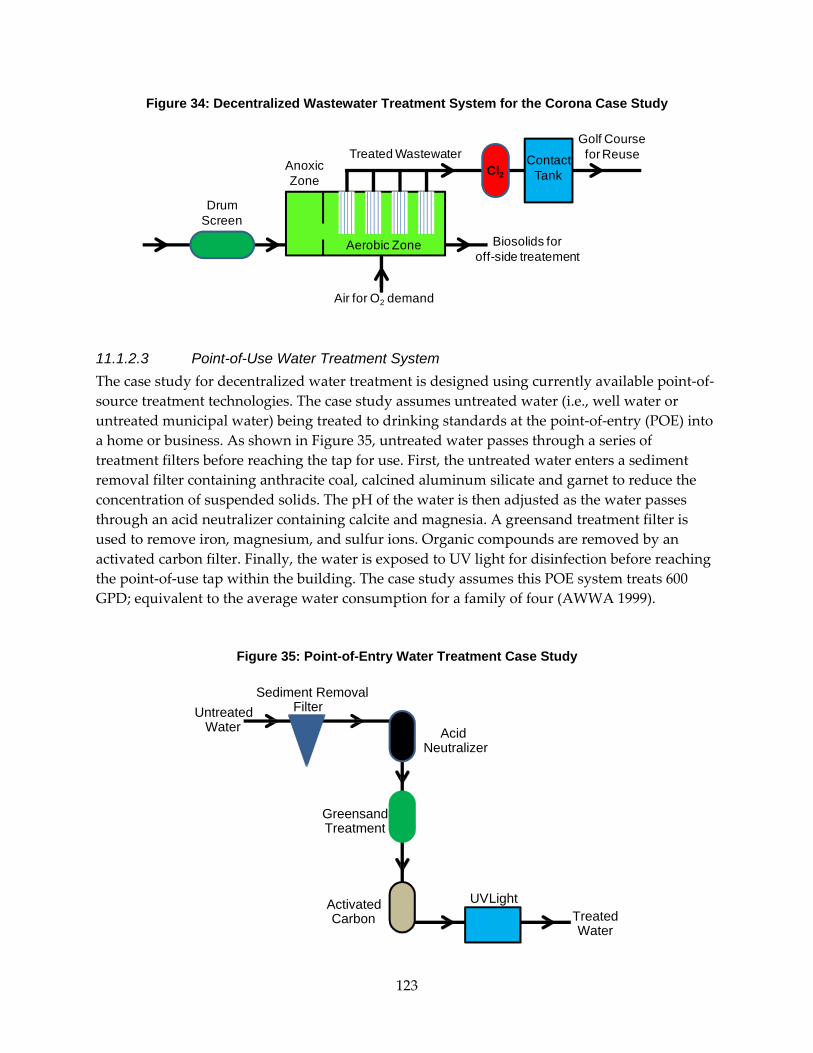
123

Figure 34: Decentralized Wastewater Treatment System for the Corona Case Study

11.1.2.3 Point-of-Use Water Treatment System The case study for decentralized water treatment is designed using currently available point‐of‐source treatment technologies. The case study assumes untreated water (i.e., well water or untreated municipal water) being treated to drinking standards at the point‐of‐entry (POE) into a home or business. As shown in Figure 35, untreated water passes through a series of treatment filters before reaching the tap for use. First, the untreated water enters a sediment removal filter containing anthracite coal, calcined aluminum silicate and garnet to reduce the concentration of suspended solids. The pH of the water is then adjusted as the water passes through an acid neutralizer containing calcite and magnesia. A greensand treatment filter is used to remove iron, magnesium, and sulfur ions. Organic compounds are removed by an activated carbon filter. Finally, the water is exposed to UV light for disinfection before reaching the point‐of‐use tap within the building. The case study assumes this POE system treats 600 GPD; equivalent to the average water consumption for a family of four (AWWA 1999).

Figure 35: Point-of-Entry Water Treatment Case Study

Aerobic Zone

AnoxicZone

DrumScreen

Treated WastewaterCl2

ContactTank

Golf Coursefor Reuse

Biosolids for off-side treatement

Air for O2 demand

Sediment RemovalFilter

AcidNeutralizer

UV Light

GreensandTreatment

ActivatedCarbon Treated

Water

UntreatedWater

124

11.2 Task 11 Outcomes 11.2.1 Stonehurst Outcomes

Energy and GHG results for the Stonehurst decentralized wastewater system are presented in Figure 36. Energy use and GHGs for hypothetical centralized wastewater utility in California (see Chapter 10) are compared in Figure36. Figure shows the Stonehurst case study requires about five times more energy than the larger centralized system (labeled as “Centralized”). Specifically, the Stonehurst system uses about 125 GJ of energy for every MG treated wastewater while the Centralized system uses about 25 GJ. A similar magnitude difference is observed between the two treatment systems for GHGs, with one MG of treated wastewater at the Stonehurst site resulting 12 Mg of GHG emissions while only about 2 Mg are associated with the Centralized utility.

Figure 36: Energy and GHG Emissions Summary

Values represent GJ for energy and Mg of GHGs per MG of treated wastewater.

Figures 37 ‐ 39 disaggregate the WWEST energy results for both the Stonehurst and Centralized treatment system into wastewater phases, life‐cycle phases, and activity, respectively. Separating energy use by wastewater phase, as shown in Figure 37, illustrates that treatment at Stonehurst represents about half of all energy use and the other half is divided between the collection and discharge phases. Collection and discharge of the water supply phase for the Centralized wastewater treatment, however, are relatively insignificant with treatment representing nearly all the energy use. While the low impact of collection and discharge may be due to economies of scale with such a large utility, this low impact may also be due to locally owned and operated collection infrastructure are not included in the Centralized case study

0

25

50

75

100

125

Energy GWP

Stonehurst Centralized

125

(Stokes and Horvath 2010). Figure 38 shows that operation demands the greatest amount of energy for both the Stonehurst and Centralized system. The energy associated with construction, and to a lesser extent maintenance, in the Stonehurst case study, however, is significant, while the operation phase represents nearly all energy use for the Centralized system. Figure 39 disaggregates energy use by activity and indicates that energy production (representing electricity generation) is the greatest contributor to the energy use for Stonehurst, followed by material production and equipment use. Figure 39 also shows that energy use for the Centralized system is fairly evenly divided between energy production and material production, while energy associated with equipment use is relatively minor.

Figure 37: Water Supply Phase Energy Use

Energy use (GJ) per MG for Stonehurst (left) and centralized system (right). Note the difference in scale.

Figure 38: Life-Cycle Phase Energy Use

Energy use (GJ) per MG for Stonehurst (left) and centralized wastewater system (right). Note the difference in scale for Stonehurst and centralized treatment results.

0

10

20

30

40

50

60

70

80

Collection Liq. Treatment

Sol. Treatment

Discharge

Water Supply Phase

0

5

10

15

20

25

Collection Liq. Treatment Sol. Treatment Discharge

Water Supply Phase

0

10

20

30

40

50

60

70

80

Construction Operation Maintenance End-of-life

Life-cycle Phase

0

5

10

15

20

25


Life-cycle Phase

126

Figure 39: Activity Phase Energy Use

Energy use (GJ) per MG for Stonehurst (left) and centralized wastewater system (right). Note the

difference in scale.

Figures 40 ‐ 42 disaggregate the GHG emissions for the Stonehurst and Centralized systems into wastewater phases, life‐cycle phases, and activities, respectively. Figure 40 shows the GHG emissions from liquid treatment at Stonehurst are greatest, though GHG emissions from collection, solid treatment, and discharge are still significant. Results for GHG emissions for the Centralized system show that liquid treatment accounts for nearly all of the GHG emissions. Figure 41 shows that the distribution of GHG emissions by life‐cycle phase is fairly similar for both the Stonehurst and Centralized systems, with most emissions occurring during the operation phase. Figure 42, which separates GHG emissions by activity, shows that direct emissions account for nearly half of all the GHGs released from the Stonehurst system while direct emissions are a minor contribution for the Centralized system. This significant disparity is due to CH4 released from the septic tanks and from solid disposal in the Stonehurst system. Alternatively, the CH4 emissions from the centralized wastewater treatment plant occur at the treatment facility and are assumed to be effectively controlled (Stokes and Horvath 2010).

0

10

20

30

40

50

60

70

80


Sol. Treatment

Discharge

Water Supply Phase

0

5

10

15

20

25

MaterialProduction

MaterialDelivery

Equipmentuse

Energyproduction

Disposal

Activity

127

Figure 40: Water Supply Phase GHG Emissions

GHGs in Mg per MG for Stonehurst (left) and centralized system (right). Note the scale difference.

Figure 41: Life-Cycle Phase GHG Emissions

GHGs in Mg per MG for Stonehurst (left) and centralized system (right). Note scale difference.

0

3

6

9


Sol. Treatment

Discharge

Water Supply Phase

0.0

0.4

0.8

1.2

1.6


Sol. Treatment

Discharge

Water Supply Phase

0

3

6

9


Life-cycle Phase

0.0

0.4

0.8

1.2

1.6


Life-cycle Phase

128

Figure 42: GHG Emissions by Activity

GHGs (Mg) for Stonehurst (left) and centralized system (right) per MG. Note the scale difference.

Figure 43 presents WWEST results for air pollutant emissions, specifically NOx, PM, SOx, and VOC, from both the Stonehurst and the Centralized wastewater system. Similar to the energy and GHG results, the air pollutant emissions from wastewater treatment at the Stonehurst site are approximately an order of magnitude greater than the emissions from the Centralized system for a given functional unit. Along with the absolute difference between the two wastewater systems, the results also show a difference between the relative pollutant emissions. The relatively greater emissions of NOx and PM at the Stonehurst site, compared to the Centralized system, indicate a greater impact from emissions associated tailpipe emissions from vehicles and equipment. The dominant NOx and SOx emissions at the centralized plant indicate that the majority of the air pollutants released are associated with electricity generation.

Figure 43: Air Pollutant Emissions Summary

Air pollutant emissions for Stonehurst and centralized systems in kg per MG of treated wastewater.

0.0

0.4

0.8

1.2

1.6

MaterialProduction

MaterialDelivery

Equipmentuse

Energyproduction

Disposal DirectEmissions

Activity

129

Figures 44 ‐ 46 disaggregate the WWEST air pollutant emission results for both the Stonehurst and Centralized treatment system into water supply phases, life‐cycle phases, and activity, respectively. Figure 44 shows that the distribution of air pollutants among the collection, liquid treatment, and discharge phases at the Stonehurst site is similar in proportion to the energy use distribution in Figure 44. The relative emissions for each air pollutant are fairly equal for each water supply phase at the Stonehurst site. Results for the Centralized plant show that most of the air pollutants occur during treatment and that these pollutant emissions are dominated by NOx and SOx, indicating that the majority of these air pollutant emissions may be associated with electricity generation.

Figure 45 presents the distribution of air pollutants between different life‐cycle phases and shows that most emissions occur during the construction and operation phases for both the Stonehurst and the Centralized plant. The distribution of air pollutants indicates that most of these emissions are associated with construction, though a significant amount of PM occurs during the operation phase. The relative emission for both the construction and operation phase at the Centralized plant are indicative of emission associated with electricity production. Figure 46, shows that significant PM emissions at the Stonehurst site occur during energy production. Along with energy production, air pollutant emissions are primarily associated with material production for both the Stonehurst and Centralized systems. Air pollutants emissions, specifically NOx, are also significant from equipment use in the Stonehurst system.

Figure 44: Water Supply Phase Air Pollutant Emissions

Air pollutant emissions (kg per MG) for Stonehurst (left) and centralized system (right). Note the

difference in scale for Stonehurst and centralized treatment results.

130

Figure 45: Life-Cycle Phase Air Pollutant Emissions

Air pollutant emissions (kg per MG) for Stonehurst (left) and centralized system (right). Note scale

difference.

Figure 46: Air Pollutant Emissions by Activity

Air pollutant emissions (kg per MG) for Stonehurst (left) and centralized system (right). Note the difference in scale.

11.2.2 Corona Outcomes

Energy and GHG results for the Corona MBR treatment plant are presented in Figure 47. These results represent only the treatment phase of the wastewater treatment process (i.e. results do not include collection or disposal). Figure 47 compares energy consumption and GHG emissions of the Corona MBR treatment with the wastewater treatment phase at the Centralized plant (conventional process train) and at Stonehurst. The calculations show that the MBR treatment in the Corona case study consumes 52 GJ for every MG of treated wastewater, which is similar to the 57 GJ required at Stonehurst but more than the 17 GJ needed at the Centralized system. A similar trend is observed when comparing the treatment phase of each case study for

131

GHGs, with one MG of treated wastewater resulting 10 Mg, 1 Mg, and 9 Mg of GHG emissions for the Corona, Centralized, and Stonehurst case studies, respectively.

Figure 47: Treatment Phase Energy and GHGs Summary

Energy (GJ) and GHG (Mg) per MG comparison of the treatment phase of the Stonehurst, Centralized, and Corona systems.

Figures 48 and 49 disaggregate the WWEST treatment phase energy results for both the Corona and Centralized treatment systems into life‐cycle phases and activity, respectively. Figure 48 shows that operation stage demands the greatest energy for both the Corona and Centralized systems. The energy associated with construction and maintenance at the Corona plant, however, is still significant, while the operation phase represents nearly all energy use for the Centralized treatment process. Figure 49 disaggregates treatment phase energy use by activity and indicates that energy and material production together require nearly all of the energy consumed throughout the lifecycle for the Corona case study, while material delivery, equipment use, and disposal are relatively nominal. This distribution of lifecycle energy is also observed for treatment phase energy use at the Centralized system.

132


Treatment energy use (GJ per MG) of the Corona (left) and Centralized system (right). Note the difference in scale.


Treatment energy use (GJ per MG) of the Corona (left) and centralized system (right). Note the difference in scale.

Figures 50 and 51 disaggregate GHG emissions for treatment at the Corona and Centralized treatment systems into life‐cycle phases and activity, respectively. Figure 50 shows that the distribution of GHG emissions by life‐cycle phase is similar for wastewater treatment at both the Corona and Centralized plant, with most emissions occurring during the operation phase. Figure 51, which separates GHG emissions by activity, shows that direct emissions account for more than half of all the GHGs released at the Corona plant while direct emissions are a minor contribution to the treatment phase emissions for the Centralized system. While CH4 emission are effectively controlled at the Centralized plant (Stokes and Horvath 2010), the large amount

0

10

20

30

40


Life-cycle Phase

0

5

10

15

20


Life-cycle Phase

0

10

20

30

40

MaterialProduction

MaterialDelivery

Equipmentuse

Energyproduction

Disposal

Activity

0

5

10

15

20

MaterialProduction

MaterialDelivery

Equipmentuse

Energyproduction

Disposal

Activity

133

of direct emissions in the Corona case studyare the result of assuming no methane flaring at this small MBR plant.


GHGs (Mg) per MGfor the treatment phase of the Corona (left) and centralized (right) wastewater system. Note the order-of magnitude difference in scale for Corona and Centralized results.

Figure 51: GHG Emissions by Activity

GHGs (Mg) for the treatment phase of the Corona (left) and centralized (right) system. Note the order-of magnitude difference in scale for Corona and Centralized treatment results.

0

3

6

9

12


Life-cycle Phase

0.0

0.3

0.6

0.9

1.2


Life-cycle Phase

0

3

6

9

12

MaterialProduction

MaterialDelivery

Equipmentuse

Energyproduction


Activity

0.0

0.3

0.6

0.9

1.2

MaterialProduction

MaterialDelivery

Equipmentuse

Energyproduction


Activity

134

Figure 52 presents WWEST results for air pollutant emissions, specifically NOx, PM, SOx, and VOC released during the treatment phase for both the Corona and the Centralized WWTPs. The air pollutant emissions at the Corona and the Centralized plants are comparable, with the Corona emissions slightly higher for each of the pollutants except SOx. Stonehurst treatment emissions are considerably higher than the other case studies for all air pollutants calculated.

Figure 52: Treatment Phase Air Pollutant Emissions Summary

Air pollutant emission (kg) per MG comparison of the treatment phase of the Stonehurst, Centralized, and Corona treatment systems.

Figures 53 and 54 disaggregate the WWEST air pollutant emission results for the treatment phase at both the Corona and Centralized treatment plants into life‐cycle phases and activity, respectively. Figure 53 presents the distribution of air pollutants between life‐cycle phases. At the Corona plant most PM, SOx, and NOx emissions occur during the operation phase. VOC emissions are fairly evenly distributed among the construction, operation, and maintenance life‐cycle phases. SOx emissions at the Centralized plant mostly occur during operation. Similar emission levels of the other air pollutants at the Centralized plant occur between the construction and operation phases. Figure 54, shows that the PM, SOx, and NOx emissions are the result of electricity generation. The treatment air emissions at the Centralized plant are relatively low and similarly distributed among the energy and material production activities.

135


Air pollutant emissions (kg) per MG for the Corona (left) and Centralized (right) WWTPs. Note the difference in scale for Corona and Centralized treatment results.


Air pollutant emissions (kg) per MG for the Corona (left) and Centralized (right) WWTPs. Note the difference in scale for Corona and Centralized treatment results.

11.2.3 Point-of-Entry Outcomes

Energy and GHG results for the POE water treatment case study are presented in Figures 55a and 55b. These results represent only the treatment phase (i.e. results do not include supply or distribution. Figures 55a and 55b also present, for comparison, the energy consumption and GHG emissions from the water treatment at a large centralized water treatment utility in California (Stokes and Horvath 2011; see Chapter 9). The calculations show that the POE water treatment consumes 65 GJ for every MG of treated water, which is considerably greater than the 5 GJ needed at the Centralized system. A similar trend is observed when comparing the water treatment from each case study for GHGs, with one MG of treated water resulting 3 Mg of GHG

136

emissions for the POE water treatment case study while the Centralized system emits an order of magnitude less, 0.3 Mg.

Figure 55a and 55b: Water Treatment Energy and GHGs Summary

Energy (MJ) and GHGs (Mg) per MG comparison for a POE and Centralized water treatment system. Note the scale difference.

Figures 56 and 57 disaggregate the results for water treatment of both the POE case study and Centralized treatment plant into life‐cycle phases and activity, respectively. While the overall energy use is significantly greater in the POE case study, Figure 56 shows a similar relative distribution of energy use among the life‐cycle phases for both the POE and Centralized systems, with the majority of energy use occurring during operation. Figure 57 disaggregates energy use by activity and indicates that energy production (representing electricity generation) is the greatest contributor of the energy use for the POE case study, with this electricity demand primarily due to UV disinfection. Figure 57 also shows that material production energy for the Centralized system is fairly equal to the energy production, due to the relatively large amount of energy required in the production of treatment chemicals.

010203040506070

Energy

POE Centralized

012345

GWPPOE Centralized

137


Energy use (GJ) per MG of the POE case study (left) and Centralized system (right).Note the difference in scale.


Energy use (GJ) per MG of the POE case study (left) and Centralized water treatment system (right). Note the scale difference.

Figures 58 and 59 disaggregate the GHG results for both the POE case study and Centralized water treatment systems into life‐cycle phases and activity, respectively. Figure 58 shows that GHG emissions follow a similar trend to the life‐cycle phase disaggregated energy use in Figure 56, with most GHG emissions occurring during operation for both the POE and Centralized water treatment systems. Figure 59, which separates GHG emissions by activity, shows that emissions generated during material production become significant relative to the GHG emissions from energy production for the POE system, and GHG emissions from material production are actually greater than the GHG emissions from energy production for the Centralized system.

0

10

20

30

40

50

60

Construction Operation Maintenance

Life-cycle Phase

0

1

2

3

4

5


Life-cycle Phase

0

10

20

30

40

50

60

MaterialProduction

MaterialDelivery

Equipmentuse

Energyproduction

Activity

0

1

2

3

4

5

MaterialProduction

MaterialDelivery

Equipmentuse

Energyproduction

Activity

138

Figure 60 presents results for air pollutant emissions, specifically NOx, PM, SOx, and VOC, from both the POE case study and Centralized treatment systems. The air pollutant emissions from the POE case study are greater than the emissions from the Centralized treatment facility, though to a lesser extent than observed with the energy and GHG results. Along with the absolute difference between the two water treatment systems, the results also show a difference between the relative emissions of the pollutants. The relatively greater emissions of SOx for the POE case study indicates the dominant contribution of electricity generation, while the relatively large VOC emissions in the Centralized system is a result of the production of certain treatment chemicals (primarily ammonia and sodium hydroxide).


GHGs (kg) per MG for the POE case study (left) and Centralized water treatment system (right), separated by life-cycle phase. Note the difference in scale for POE and Centralized treatment results.

Figure 59: GHG emissions by Activity

GHGs (kg) per MG for the POE case study (left) and Centralized water treatment system (right). Note the difference in scale.

0

1

2

3

4

5


Life-cycle Phase

0.00

0.05

0.10

0.15

0.20

0.25


Life-cycle Phase

0

1

2

3

4

5

MaterialProduction

MaterialDelivery

Equipmentuse

Energyproduction

Activity

0.00

0.05

0.10

0.15

0.20

MaterialProduction

MaterialDelivery

Equipmentuse

Energyproduction

Activity

139

Figure 60: Water Treatment Air Pollutant Emissions Summary

Air pollutant emissions (kg) per MG comparison of the POE case study and Centralized water systems.

Figures 61 and 62 disaggregate the air pollutant emissions for both the POE and Centralized systems into life‐cycle phases and activities, respectively. The distribution of air pollutants between different life‐cycle phases confirms that most emissions occur during the operation phase for both the POE case study and Centralized plant. The distribution of air pollutants for the POE case study indicates that most of these emissions are associated with material and energy production during operation while the relatively significant amount of VOC with the Centralized plant confirms that these emission are the result of producing chemicals used in the during the operation.


Air pollutant emissions (kg) per MG for the POE case study (left) and Centralized water system (right). Note the difference in scale for POE and Centralized treatment results.

0

2

4

6

8

10

NOx PM SOx VOC CO

POE Centralized

140


Air pollutant emissions (kg per MG) for the POE case study (left) and Centralized water treatment system

(right). Note the difference in scale for POE and Centralized treatment results.

11.3 Task 11 Conclusions and Recommendations Energy, GHG, and air emissions from three wastewater treatment case studies were evaluated using the WWEST model. Results show that the economies of scale with Centralized plant outweigh the impact benefits gained from both the low energy (Stonehurst) and high technology (Corona) decentralized case studies. The Centralized facility also benefits from flaring methane generated during the treatment process while CH4 was assumed to be directly emitted in the decentralized systems.

The WEST model was used to compare energy, GHG, and airemissions from a POE case study and a centralized water treatment facility. The results indicate that the economies of scale associated with a Centralized facility result in lower energy use and emissions. While Centralized water treatment impacts are normalized across a large volume of water, POE system only treats household water demand. Furthermore, most of impacts from the POE system are fixed regardless of variation in household demand so that conservation efforts, at the household level, would provide minimal benefit. The results show that energy and emissions associated with the POE case study are primarily due to energy production required for the operation UV lighting. Alternative forms of POE disinfection may reduce the environmental impact on household water treatment.

141

CHAPTER 12: Project Summary This chapter summarizes the project MR‐06‐08, completed between October 15, 2006 and December 31, 2010. The project consisted of eleven tasks:

• Task 1: Administration. Consisted primarily of tracking project activities, documenting, reporting, communicating with the Energy Commission, and budgeting over the project period.

• Task 2: Assess alternative energy sources. Edited WEST to allow the user to enter customized electricity mixes.

• Task 3: Consider additional water sources. Revised the tool to be used to analyze any water source or alternative scenario.

• Task 4: Calculate EFs for common materials. Evaluated the life‐cycle emissions for common material choices in water systems, including pipe materials and tank design.

• Task 5: Include life‐cycle effects of electricity generation. Updated WEST to allow the user to analyze California water systems using life‐cycle EFs for electricity production.

• Task 6: Evaluate demand management measures. Quantified the effects of reducing water demand through conservation programs.

• Task 7: Consider additional pollutants. Expands the pollutants analyzed to include additional air emissions as well as water and land pollutants.

• Task 8: Develop workshops for industry professionals. Involved planning and presenting WEST and WWEST to industry professionals during two workshops, one in Southern California and one in Northern California.

• Task 9: Improve material production analysis. Provided more detailed analysis of certain materials not well‐defined using EIO‐LCA (the tool choice in Phase One of the project), especially chemicals and plastics. Data were obtained from publicly‐ and commercially‐available sources.

• Task 10: Analyze the energy demand of wastewater systems. Created a separate decision support tool, WWEST, and evaluated a case study system.

• Task 11: Evaluate decentralized water and wastewater systems. Updated WEST and WWEST to evaluate decentralized water and wastewater case studies.

Each task is described in detail in a preceding chapter. This chapter provides some combined context for the outcomes from the various tasks and case studies that were part of this project.

142

12.1 Project Outcomes The following describes the outcomes of the overall project, including a summary of major deliverables and outcomes from the case study analyses.

12.1.1 Deliverables

Table 56 summarizes the deliverables for the project, including which task or tasks are associated and where the deliverable can be located. Future updates to the tools and documentation will be available at http://west.berkeley.edu/model.php.

Table 56: Project Deliverables

Task(s) Deliverable Location NotesRevised WEST Tool

Appendix A.1.1 The tool was revised several times throughout the project duration & was submitted with project Progress Reports as each task was due. The final version is included herein.

WEST Documentation

Appendices A.1.2, A.1.3, A.1.4

The appendix includes the user manual, revision log, & copies of the explanatory/help worksheets.

2 Desalination Comparison

Chapter 3 The case study analyzes a hypothetical desalination system in Coastal California.

3 Northern California Case Study Report

Chapter 4 The authors reanalyzed the results of a Phase One Northern California utility, including reservoir water that provides the majority of the utility's water supply but was previously excluded.

WESTLite Tool Appendix E.1 The WESTLIte tool analyzes which piping material & tank design are environmentally preferable to establish baseline EFs for common uses of these materials in water supply.

WESTLite Documentation

Appendix E.2 The appendix includes the Explanatory/Help worksheets from the WESTLite tool.

Planning guidelines for common materials

Chapter 5 The outcomes for Task 4 include tables which describe which common materials are environmentally preferable under various conditions (e.g., pipe diameter, tank capacity).

5 Northern & Southern California Case Study Report

Chapter 6 The researchers reanalyzed Phase One utilities (NC-Current, NC-Proposed, & SC) including the life-cycle effects of electricity generation & sludge disposal.

6 Comparison of conservation & water supply

Chapter 7 The outcomes compared results from the NC-Proposed water supply option to conservation programs (i.e., indoor & outdoor options for residential & other customers).

7 Desalination Results Report

Chapter 8 A hypothetical scenario for providing desalinated water to California's major cities was analyzed using the updated WEST.

8 Workshop Materials

Appendix G The appendix includes copies of the slides for two workshops, one in Northern & one in Southern California.

9 Case Study Results

Chapter 10 The authors analyzed two additional case studies in Northern California, one small & one large.

WWEST Tool Appendix A.2.1 The final version of WWEST is included in the appendix.WWEST Documentation

Appendices A.2.2, A.2.3, A.2.4

The appendix includes the user manual, revision log, & copies of the explanatory/help worksheets.

Wastewater utility case study results

Chapter 11 A large wastewater utility was analyzed using WWEST. This utility captures methane to produce electricity to run their plant. A typical hypothetical utility was analyzed for comparison.

11 Decentralized Water & Wastewater Case Study Results

Chapter 12 Two decentralized wastewater scenarios were analyzed. One uses septic tanks followed by secondary treatment. The other incorporates membrane bioreactors (MBRs). One residential point-of-entry water system was also analyzed.

2, 3, 5, 7, 9

4

10

143

12.1.2 Water System Case Studies

After all the revisions were made to WEST, the researchers reanalyzed all case studies collected up to that date using the same analysis parameters. The functional unit was one Ml and the analysis period was 25 years. All case studies were then compared on an equal basis to see better how different utilities and water sources performed using LCA. Table 57 summarizes these utilities and water sources analyzed.

Table 57: Project Case Study Summary

Table 58 shows the energy, GHG, and NOx results for each of the five case study utilities described above, assuming the water source mix shown in Table 58.

Table 58: California Utility Results Summary

On a systemwide basis, the NC‐Small utility consistently results in higher environmental burden, more than twice the other systems in most cases. Two factors may contribute to this outcome: 1) the significant amount of electricity needed to pump groundwater, the sole source of water for this system; or 2) economies of scale. The other analyzed utilities all produce more

Sources (%)

System LocationProduction (Ml/year) Im

port

edLo

cal

surf

ace

wat

er

Gro

und-

wat

er

Brac

kish

De

sal

Seaw

ater

De

sal

Recy

cled

NC-Small Northern California 6700 100%NC-Current Northern California 38000 26% 72% 2%NC-Proposed Northern California 38000 72% 26% 2%SC Southern California 41000 92% 8% <1%NC-Large Northern California 280000 95% 5%Note: The electricity consumption values for the NC-Current and NC-Proposed systems were analyzed using the revised electricity consumption values discussed in Task 3 (see Chapter 4.) The SC recycled water electricity values were similarly revised using estimates from (Energy Commission 2005).

UtilityEnergy (GJ/Ml)

GHGs (Mg/Ml)

NOx

(Mg/Ml)NC-Small 20 1.4 0.0035NC-Current 6.4 0.32 0.00045NC-Proposed 16 0.83 0.00083SC 16 0.75 0.00086NC-Large 5.6 0.33 0.00089

144

than five times the water produced in the NC‐Small case. Groundwater energy use is primarily related to water depth and will vary significantly based on site conditions.

The NC‐Proposed and SC case studies showed similar results. NC‐Proposed implements a seawater desalination which is energy intensive, though it only makes up 26 percent of the water supply. SC, on the other hand, uses a less‐intensive form of desalination, brackish groundwater, for 8 percent of their supply. However, the majority of SC’s water is imported through the SWP and CRA, both energy‐intensive sources.

The NC‐Current and NC‐large utilities have the lowest environmental effects, according to this analysis. NC‐Current primarily uses local surface water combined with imported water that does not require much treatment. NC‐Large imports most of its water (95 percent) but the aqueducts are gravity‐fed, making it an energy‐efficient water source.

Figure 63 compares the energy results for all the water sources evaluated independently. This figure confirms the conclusions described above. The NC‐Small groundwater results are comparable to SC’s brackish groundwater system. NC‐Proposed’s desalination system results in twice the energy use of any other source.

Figure 63: Comparison of Energy Demand of Various Water Sources

Recycled water is shown to be environmentally preferable in both of the systems analyzed. However, it is not significantly better than the NC‐Large’s imported water. However, not all environmental effects are included in the results. Notably, the impacts of water withdrawal on ecological receptors (e.g., habitat) or on long‐term source sustainability (i.e., ensuring recharge

0

10

20

30

40

50

NC‐Cu

rrent

SC

NC‐Large

NC‐Cu

rrent

NC‐Large

NC‐Sm

all

SC

NC‐Proposed

NC‐Cu

rrent

SC

Imported Local Surface

GW Desal Recycled

Energy

(GJ/million liters)

145

is equal to or greater than withdrawals) are not included. Including these ecological effects would likely penalize all results except recycled water.

12.1.3 Wastewater System Case Studies

Energy, GHG, and pollutant emissions from three wastewater treatment case studies were evaluated using the WWEST model. Results from WWEST in Tables 59 and 60 show that the economies of scale with Centralized wastewater treatment outweigh the impact benefits gained from both the low energy (Stonehurst) and high technology (Corona) decentralized wastewater treatment case studies.

Table 59: Wastewater Case Study Summary

Table 60: Wastewater Case Study Summary (treatment only)

12.2 Project Conclusions The project conclusions are presented in two categories: Tools and Case Studies. General recommendations for research into the energy‐water connection and the environmental impacts of water and wastewater systems are also discussed.

12.2.1 Tools

Conclusions related to WEST, WESTLite, and WWEST are listed below:

Results Centralized StonehurstEnergy (GJ) 26 122GHG (Mg) 2 12Nox (kg) 2 19

PM (kg) 0 15SOx (kg) 10 10

VOC (kg) 29 8CO (kg) 11 30

Results Centralized Stonehurst CoronaEnergy (GJ) 17 57 52GHG (Mg) 1 9 10Nox (kg) 1 10 3PM (kg) 0 6 7SOx (kg) 3 7 2VOC (kg) 1 5 3CO (kg) 11 26 9

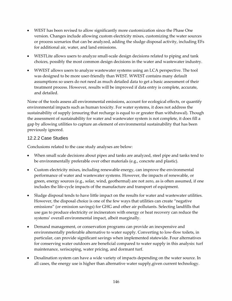
146

• WEST has been revised to allow significantly more customization since the Phase One version. Changes include allowing custom electricity mixes, customizing the water sources or process scenarios that can be analyzed, adding the sludge disposal activity, including EFs for additional air, water, and land emissions.

• WESTLite allows users to analyze small‐scale design decisions related to piping and tank choices, possibly the most common design decisions in the water and wastewater industry.

• WWEST allows users to analyze wastewater systems using an LCA perspective. The tool was designed to be more user‐friendly than WEST. WWEST contains many default assumptions so users do not need as much detailed data to get a basic assessment of their treatment process. However, results will be improved if data entry is complete, accurate, and detailed.

None of the tools assess all environmental emissions, account for ecological effects, or quantify environmental impacts such as human toxicity. For water systems, it does not address the sustainability of supply (ensuring that recharge is equal to or greater than withdrawal). Though the assessment of sustainability for water and wastewater system is not complete, it does fill a gap by allowing utilities to capture an element of environmental sustainability that has been previously ignored.

12.2.2 Case Studies

Conclusions related to the case study analyses are below:

• When small scale decisions about pipes and tanks are analyzed, steel pipe and tanks tend to be environmentally preferable over other materials (e.g., concrete and plastic).

• Custom electricity mixes, including renewable energy, can improve the environmental performance of water and wastewater systems. However, the impacts of renewable, or green, energy sources (e.g., solar, wind, geothermal) are not zero, as is often assumed, if one includes the life‐cycle impacts of the manufacture and transport of equipment.

• Sludge disposal tends to have little impact on the results for water and wastewater utilities. However, the disposal choice is one of the few ways that utilities can create “negative emissions” (or emission savings) for GHG and other air pollutants. Selecting landfills that use gas to produce electricity or incinerators with energy or heat recovery can reduce the systems’ overall environmental impact, albeit marginally.

• Demand management, or conservation programs can provide an inexpensive and environmentally preferable alternative to water supply. Converting to low‐flow toilets, in particular, can provide significant savings when implemented statewide. Four alternatives for conserving water outdoors are beneficial compared to water supply in this analysis: turf maintenance, xeriscaping, water pricing, and dormant turf.

• Desalination system can have a wide variety of impacts depending on the water source. In all cases, the energy use is higher than alternative water supply,given current technology.

147

• Wastewater system results can be significantly improved by using methane to offset other electricity supplies. For the case study utility herein, the plant is able to meet approximately 90 percent of its electricity needs using captured CH4. The utility plant’s GHG was 435 Mg per MG less than the potential emissions from the hypothetical plant.

• The economies of scale associated with centralized water and wastewater treatment plants results in lower energy requirements, for a given amount of treated water, relative to decentralized systems compared in this report.

• Case study results are site‐specific and will vary by geography, hydrology, system design, water sources, and other factors. The case study results in this report can be used as guidance, but may not be directly applicable to other utilities.

12.3 Project Recommendations The primary recommendation of this research is that WEST and WWEST should be introduced to utilities to educate them about the tools themselves and, perhaps more importantly, about life‐cycle thinking itself. Utilities should be encouraged to take a long‐term and life‐cycle perspective on energy use and environmental emissions, including indirect emissions associated with the supply chain. LCA should be encouraged for design and planning of new water and wastewater systems and major system expansions and retrofits.

Other, more specific recommendations are summarized here:

• Desalination is an oft‐discussed alternative for coastal water systems wanting a flexible and reliable water source. However, the energy and environmental effects should be accounted for in decision making. If implemented in several large cities, the impact on the state’s energy supplies will be significant.

• Some wastewater treatment processes allow opportunities for heat and energy recovery which can offset fossil fuel consumption and prevent GHG emissions. Anaerobic treatment processes which produce CH4 are particularly good candidates.

• Disposal choices may also be important for water and wastewater systems that want to limit environmental burden. Offsets with fuel or electricity consumption or generation as well as other materials (e.g., fertilizers) can be important to limiting the system’s effect on the environment.

• California’s climate change regulations are ground‐breaking and encouraging for those concerned about long‐term environmental health. However, this research shows that analyzing climate change effects requires a broader vision than the reporting required currently by the legislation.

• The interest in this research at the two workshops conducted as part of this work indicate that the researchers, and the Energy Commission, should keep the participants, and other interested parties, apprised of the latest research and tools available for evaluating these issues after this contract ends.

148

Water and wastewater design decisions are made based on several factors, including economic, engineering, and political concerns. The comprehensive and systemwide life‐cycle environmental effects of the water infrastructure have not been a factor in these decisions. Generally, utilities, designers, and system planners are not aware that it is possible to assess the environmental effects of their systems using LCA; as a result, the analysis is not included in decision‐making.

For a more comprehensive picture of the costs associated with water supply choices, LCA using WEST, WWEST, or similar methodology should be conducted routinely. This would allow the industry to develop a comprehensive list of design recommendations for systems of differing parameters (e.g., scale, water quality, process selection). The model and tools described herein will allow utilities and other planners to incorporate these effects into their decision processes, and with more informed analyses strive for sustainable solutions.

149

GLOSSARY

Term Definition

AC Asbestos cement AF AF AF acre-foot Assump Assumption worksheet designation AWWA American Water Works Associate Calc Calculation worksheet designationCBOD Carbonaceous oxygen demand CH4 Methane CI Cast iron CIEE California Institute for Energy and Environment CII Commercial, Institutional, and Industrial sector CO Carbon monoxide CO2(e) Carbon dioxide equivalents COL Collection COM Scenario: A commercial facility (i.e., big box store) in the desert region Conv Conversion worksheet designation CRA Colorado River Aqueduct d Day DEF Default calculation worksheet designation DI ductile iron DIS Distribution (water) or discharge (wastewater) EBMUD East Bay Municipal Utility District EF Emission factor EGRID Emissions and Generation Resource Integrated Database EIO-LCA Economic Input-Output Analysis-based LCA Energy C i i

California Energy Commission EP Energy production activity EU Equipment use activity FEPA Federal Energy Policy Act g gram g/kWh grams per kilowatt-hour gal Gallon GHG greenhouse gas GJ Gigajoules gpd Gallons per day gpd gallons per day gpm gallons per minute GREET Greenhouse Gases, Regulated Emissions, and Energy Use in Transportation GWE Global warming effect GWP Global warming potential HC Hydrocarbons

150

hh Household in Inch IND Scenario: A 40,000 m2 (10-acre) industrial site in the central region ISO International Organization of Standardization kl or kl Kiloliter km Kilometer LCA Life-cycle Assessment lpf Liters per flush lpm Liters per minute LTRT Liquid treatment (wastewater) m2 Square meters m3 Cubic meter MBR Membrane bioreactor MD Material delivery activity MF Scenario: A hypothetical multi-family unit in the coastal region Mg Million grams MG Million gallons mg/l milligrams per liter MGD Million gallons per day MJ Megajoules Ml or Ml Million liters MMWD Marin Municipal Water District MP Material production activity MSW Municipal solid waste MWh Megawatt-hours N2O Nitrous oxide NA Not available NC-Current Northern California case study utility (Current Water Supply) NC-Proposed Northern California case study utility (Proposed Water Supply)

NMVOCs Non-methane volatile organic compounds NOx Nitrogen oxides NREL National Renewable Energy Laboratory OWD Oceanside Water District PE Polyethylene PIER-EA Public Interest Energy Research- Environmental Area POE Point of entry PM Particulate matter PV Photovoltaics PVC Polyvinyl chloride PVDF Polyvinylidene flouride RO Reverse osmosis SC Southern California case study utility SD Sludge disposal activity

151

SETAC Society for Environmental Toxicology and Chemistry SF1 Scenario: An average-sized single family home and lot in the coastal region SF2 Scenario: An average single family home and lot in the inner coastal region SF3 Scenario: An average sized single-family home and lot in the desert region SF4 Scenario: A single family home on a large lot in the central region SOx Sulfur oxides SPU Seattle Public Utility STRT Sludge treatment (wastewater) SWP State Water Project Tg Teragrams TJ Terajoules TRT Treatment TWD Tampa Water Department U.S. EPA United States Environmental Protection Agency UV Ultraviolet VOC Volatile organic compounds WEST Water-Energy Sustainability Tool WWEST Wastewater-Energy Sustainability Tool WWTP wastewater treatment plant yr Year

152

REFERENCES

Allen, C. and E. Vonghia (2009). “Sustainable Development through Decentralized Water Reuse Technology.” Proceedings of 2009 WateReuse California Conference.

ASE (2002). “Watergy: Taking Advantage of Untapped Energy and Water Efficiency Opportunities in Municipal Water Systems.” Washington, D.C., Alliance to Save Energy/USAID.

American Society of Civil Engineers (2009). “ASCE’s Infrastructure Report Card Gives Nation a D, Estimates Costs at $2.2 Trillion.” ASCE Journal 34(2). http://www.asce.org/PPLContent.aspx?id=2147484137

Aquacraft (2005). “Water and Energy Savings from High Efficiency Fixtures and Appliances in Single Family Homes: Volume 1.” Boulder, Colorado.

AWWA (1999) American Water Works Association Research Foundation, “Residential End Uses of Water Study.” Retrieved October 1, 2010 from www.waterresearchfoundation.org

Beavis, P. and S. Lundie (2003). ʺIntegrated Environmental Assessment of Tertiary and Residuals Treatment ‐ LCA in the Wastewater Industry.ʺ Water Science and Technology 47(7‐8): 109‐116.

CEC (2005). “Californiaʹs Water‐Energy Relationship.” Sacramento, CA, California Energy Commission.

CEC (2008). “Process Energy ‐ Water/Wastewater Efficiency.” California Energy Commission. Retrieved October 7, 2008, from www.energy.ca.gov/process/water/index.html.

CARB (2002). ʺOff‐Road Emissions Model.ʺ Retrieved May 1, 2002, from www.arb.ca.gov/msei/msei.html.

Carnegie Mellon University Green Design Institute (2007). ʺEconomic Input‐Output Life Cycle Assessment (EIO‐LCA).ʺ Retrieved October 23, 2007, from www.eiolca.net.

CBO (2003). United States Congressional Budget Office, “Prospects for Distributed Electricity Generation”, September. Retrieved October 7, 2007, from http://www.cbo.gov/showdoc.cfm?index=4552&sequence=4 (Accessed December 6, 2006).

Chester, M. V. and A. Horvath. (2009). “Environmental assessment of passenger transportation should include infrastructure and supply chains.” Environmental Research Letters 4: 024008.

Chester, M. V. (2008). Life‐cycle Environmental Inventory of Passenger Transportation in the United States. Unpublished Ph.D. Dissertation, Department of Civil and Environmental Engineering, University of California, Berkeley.

153

Corti, A. and L. Lombardi (2004). ʺBiomass Integrated Gasification Combined Cycle with Reduced CO2 Emissions: Performance Analysis and Life Cycle Assessment (LCA).ʺ Energy 29(12‐15): 2109‐2124.

Crites, R. (1998). “Small & Decentralized Wastewater Management Systems.” McGraw‐Hill Science/Engineering/Math. Boston, MA. ISBN‐10:0072890878

Crites, R., C. Lekven, S. Wert, G. Tchobanoglous (1997). “A Decentralized Wastewater System for a Small Residential Development in California.” The Small Flows Journal 3(1), Winter 1997.

Cuddihy, J., C. Kennedy, P. Byer (2005). ʺEnergy Use in Canada: Environmental Impacts and Opportunities in Relationship to Infrastructure Systems.ʺ Canadian Journal of Civil Engineering 32(1): 1‐15.

Curran, M. A. (1996). “Environmental Life‐cycle Assessment.” New York, McGraw‐Hill.

Denison, R. (1996). “Environmental Life‐cycle Comparisons of Recycling, Landfilling, and Incineration: A Review of Recent Studies.” Annual Review of Energy and the Environment. 21: 191‐237.

Deru, M. and P. Torcellini (2007). “Source Energy and Emission Factors for Energy Use in Buildings.” National Renewable Energy Laboratory.

Dickie, P. (2007). “Making Water‐Desalination: Option or Distraction for a Thirsty World?” Switzerland, WWF Global Freshwater Programme.

EGRID (2002) “The Emissions and Generation Resource Integrated Database (E‐GRID2002) Version 1.0, 2000 Data.” U.S. Environmental Protection Agency: Washington, D.C.

Energy Star (2007). ʺLife‐cycle Cost Estimate for Energy Star Qualified Residential Clothes Washers.ʺ Retrieved October 7, 2007, from www.energystar.gov/ia/business/bulk_purchasing/bpsavings_calc/CalculatorConsumerClothesWasher.xls.

Facanha, C. and A. Horvath (2007). ʺEvaluation of Life‐cycle Air Emission Factors of Freight Transportation.ʺ Environmental Science & Technology 41(20): 7138‐7144.

Friedrich, E. (2002). ʺLife‐cycle Assessment as an Environmental Management Tool in the Production of Potable Water.ʺ Water Science and Technology 46(Part 9): 29‐36.

GaBi (2003). ʺGaBI Software.ʺ Retrieved March 20, 2003, from http://www.gabi‐software.com.

GaBi (2005). ʺGaBI Software.ʺ Retrieved March 20, 2003, from http://www.gabi‐software.com.

Gagnon, L., C. Belanger, Y. Uchiyama. (2002). ʺLife‐cycle Assessment of Electricity Generation Options: The Status of Research in Year 2001.ʺ Energy Policy 30(14): 1267‐1278.

General Electric (2008) Corona Wastewater Treatment Plant. General Electric Water Process Technologies. Retrieved October 7, 2010 from

154

www.gewater.com/pdf/Case%20Studies_Cust/Americas/English/CS‐CORO‐MUNWW‐EN‐1106‐NA%20GE%20Logo.pdf.

Gleick, P. H. (1995). “California Water 2020: A Sustainable Vision.” Oakland, CA, Pacific Institute for Studies in Development, Environment and Security.

Gleick, P.H., D. Haasz, C. Henges‐Jeck, V. Srinivasan, G. Wolff, K. Cushing, and A. Mann (2003). “Waste Not, Want Not: The Potential for Urban Water Conservation in California.” Oakland, California, Pacific Institute for Studies in Development, Environment, and Security: 176.

Graedel, T. E. and B. R. Allenby (2003). “Industrial Ecology.” Upper Saddle River, N.J.: Prentice Hall.

Hanak, E. (2005). “Water for Growth: Californiaʹs New Frontier.” Public Policy Institute of California: San Francisco, California.

Hanak, E. and M. Davis (2006). ʺLawns and Water Demand in California.ʺ California Economic Policy 2(2): 24.

Heller, M. C., G. A. Keoleian, M. Mann, T.A. Volk (2004). ʺLife Cycle Energy and Environmental Benefits of Generating Electricity from Willow Biomass.ʺ Renewable Energy 29(7): 1023‐1042.

Hendrickson, C., A. Horvath, S. Joshi, L. Lave (1998). “Economic Input‐Output Models for Environmental Life‐Cycle Assessment” Environmental Science & Technolog; 32, 184A‐191A.

Hendrickson, C. T., L. B. Lave, and H. Scott Matthews (2006). ʺEnvironmental Life Cycle Assessment of Goods and Services: An Input‐Output Approach.ʺ Washington, D.C.: Resources for the Future.

Herz, R. and A. Lipkow (2002). ʺLife‐cycle Assessment of Water Mains and Sewers.ʺ Water Science and Technology: Water Supply 2(4): 51.

Horvath, A. (2005). “Life‐cycle Energy Assessment of Alternative Water Supply Systems in California.” California Energy Commission, PIER Energy‐Related Environmental Research. CEC‐500‐2005‐101.

Houillon, G. and O. Jolliet (2005). ʺLife cycle assessment of processes for the treatment of wastewater urban sludge: energy and global warming analysis.ʺ Journal of Cleaner Production 13(3): 287‐299.

[IPCC] Intergovernmental Panel on Climate Change (2006). ʺ2006 IPCC guidelines for national greenhouse gas inventories.ʺ 2006, from http://www.ipcc‐nggip.iges.or.jp/public/2006gl/index.htm

John Deere. (2004). ʺConstruction Equipment.ʺ Retrieved January, 2004, from www.deere.com/en_US/cfd/construction/deere_const/crawlers/deere_dozer_selection.htm.

155

Kannan, R., K. C. Leong, R. Osmana, H.K. Ho (2007). ʺLife cycle energy, emissions and cost inventory of power generation technologies in Singapore.ʺ Renewable & Sustainable Energy Reviews 11(4): 702‐715.

Keller, J. and K. Hartley (2003). ʺGreenhouse gas production in wastewater treatment: Process selection is the major factor.ʺ Water Science and Technology 47(12): 43‐48.

Koch, F.H. (2001). “Hydropower‐Internalised Costs and Externalised Benefits” in Externalities and Energy Policy: The Life Cycle Analysis Approach. 2001. Paris, France: Nuclear Energy Agency.

Lee, K. M., S. Y. Lee, T. Hur. (2004). ʺLife cycle inventory analysis for electricity in Korea.ʺ Energy 29(1): 87‐101.

Lenzen, M. and J. Munksgaard (2002). ʺEnergy and CO2 life‐cycle analyses of wind turbines‐‐review and applications.ʺ Renewable Energy 26(3): 339‐362.

Lundie, S., G. M. Peters, P.C. Beavis. (2004). ʺLife cycle assessment for sustainable metropolitan water systems planning.ʺ Environmental Science and Technology 38(13): 3465‐3473.

Lundin, M. and G. Morrison (2002). ʺA Life Cycle Assessment Based Procedure for Development of Environmental Sustainability Indicators for Urban Water Systems.ʺ Urban Water 4: 145‐152.

Matthews, H. S. and L. B. Lave (2000). ʺApplications of Environmental Valuation for Determining Externality Costs.ʺ Environmental science & technology 34(8): 6.

Mayer, P., W. B. DeOreo, D.M. Lewis (2000). Seattle Home Water Conservation Study: The Impacts of High Efficiency Plumbing Fixture Retrofits in Single Family Homes. Boulder, Colorado, Aquacraft, Inc.

Mayer, P. W., W. B. DeOreo, E. Towler, D.M. Lewis (2003). Residential Indoor Water Conservation Study: Evaluation of High Efficiency Indoor Plumbing Fixture Retrofits in Single‐Family Homes in the East Bay Municipal Utility District Service Area. Boulder, Colorado, Aquacraft, Inc. for US Environmental Protection Agency and EBMUD: 172.

Mayer, P., W. B. DeOreo, E. Towler, L. Martien, D.M. Lewis (2004). Tampa Water Department Residential Water Conservation Study: The Impacts of High Efficiency Plumbing Fixture Retrofits in Single‐Family Homes, Aquacraft, Inc. for USEPA and Tampa Water Department.

Means, R. S. (1997). Heavy Construction Cost Data. Kingston, MA.

Means R. S. (2004). Site work and landscape cost data. Kingston, Massachusetts, R.S. Means Co.

Meier, P. (2002). Life‐cycle Assessment of Electricity Generation Systems and Applications for Climate Change Policy Analysis. Land Resources. Madison, Wisconsin, University of Wisconsin.

Metcalf and Eddy (2003). Wastewater Engineering. Boston, MA.

156

Monteith, H. D., H. R. Sahely, H.L. MacLean, D.M. Bagley (2005). ʺA rational procedure for estimation of greenhouse‐gas emissions from municipal wastewater treatment plants.ʺ Water Environment Research 77(4): 390‐403.

Murray, A., A. Hovath, K.L. Nelson (2008). ʺHybrid Life‐Cycle Environmental and Cost Inventory of Sewage Sludge Treatment and End‐Use Scenarios: A Case Study from China.ʺ Environ. Sci. Technol. 42(9): 3163‐3169.

MWD (1996). Southern Caiforniaʹs Integrated Water Resources Plan. Los Angeles, Metropolitan Water District of Southern California.

Nelson, K. L, (2005). Water Conservation, Reuse, and Recycling: Proceedings of an Iranian‐American Workshop, National Research Council Council, ed., The National Academies Press, Washington, D.C., ʺSmall and Decentralized Systems for Wastewater Treatment and Reuseʺ, January 2005.

Navigant (2006). Refining Estimates of Water‐Related Energy Use in California. Navigant Consulting, Inc. California Energy Commission, PIER Industrial/Agricultural/Water End Use Energy Efficiency Program. CEC‐500‐2006‐118.

OECD (1997). The Environmental Effects of Freight. Paris, Organization for Economic Cooperation and Development.

Ortiz, M., R.G. Raluy, L. Serra, J. Uche (2007) Life cycle assessment of water treatment technologies: wastewater and water‐reuse in a small town, Desalination 204:121–131.

Pacca, S. and A. Horvath (2002). ʺGreenhouse Gas Emissions from Building and Operating Electric Power Plants in the Upper Colorado River Basin.ʺ Environmental science & technology 36(14): 3194.

Pehnt, M. (2006). ʺDynamic life cycle assessment (LCA) of renewable energy technologies.ʺ Renewable Energy 31(1): 55‐71.

PlasticsEurope (2010). ʺEco‐profiles of the European Plastics Industry.ʺ Retrieved March 10, 2010, from http://lca.plasticseurope.org/index.htm.

Palme, U., M. Lundin, A.M. Tillman, S. Molande (2005). ʺSustainable development indicators for wastewater systems ‐ researchers and indicator users in a co‐operative case study.ʺ Resources Conservation and Recycling 43(3): 293‐311.

Rashad, S. M. and F. H. Hammad (2000). ʺNuclear power and the environment: comparative assessment of environmental and health impacts of electricity‐generating systems.ʺ Applied Energy 65(1‐4): 211‐229.

Renwick, M. E. and S. O. Archibald (1998). ʺDemand side management policies for residential water use: Who bears the conservation burden?ʺ Land Economics 74(3): 343‐359.

Riva, A., S. DʹAngelosante, C. Trebeschi (2006). ʺNatural gas and the environmental results of life cycle assessment.ʺ Energy 31(1): 138‐148.

157

Sahely, H. R., H. L. MacLean, H.D. Monteith, D.M. Bagley (2006). ʺComparison of on‐site and upstream greenhouse gas emissions from Canadian municipal wastewater treatment facilities.ʺ Journal of Environmental Engineering and Science 5(5): 405‐415.

Schleisner, L. (2000). ʺLife cycle assessment of a wind farm and related externalities.ʺ Renewable Energy 20(3): 279‐288.

Spath, P. and M. Mann (1997). Life‐cycle Assessment of a Biomass Gasification Combined Cycle Power System. Midwest Resesarch Institute, DC‐AC‐83CH10093.

Spath, P., M. Mann, and D. Kerr (1999). Cycle Assessment of Coal‐fired Power Production. Golden, Colorado, National Renewable Energy Laboratory.

Spath, P. and M. Mann (2000). Life Cycle Assessment of a Natural Gas Combined‐Cycle Power Generation System. Golden, Colorado, National Renewable Energy Laboratory.

Stokes, J. (2004). Life‐cycle Assessment of Alternative Water Supply Sources in California. Civil and Environmental Engineering. Berkeley, California, University of California: 284.

Stokes, J. and A. Horvath (2005). “Life‐Cycle Energy Assessment of Alternative Water Supply Systems.”International Journal of LCA, In print, OnlineFirst, DOI: http://dx.doi.org/10.1065/lca2005.06.214

Stokes, J. and A. Horvath (2006). ʺLife cycle energy assessment of alternative water supply systems.ʺ International Journal of Life Cycle Assessment 11(5): 335‐343.

Stokes, J. and A. Horvath (2009). ʺEnergy and Air Emission Effects of Water Supply.ʺ Environmental Science and Technology 43(8): 2680–2687.

Stokes, J. and A. Horvath (2010). ʺSupply‐chain environmental effects of wastewater utilities.ʺ Environmental Research Letters 5(1): 014015

Stokes, J. and A. Horvath (2011). ʺLife‐cycle Assessment of Urban Water Provision: A Tool and Case Study in California.ʺ Journal of Infrastructure Systems 17(1).

Suh, S. and G. Huppes (2002). ʺMissing Inventory Estimation Tool using Extended Input‐Output Analysis.ʺ International Journal of Life Cycle Assessment 7(3): 134‐140.

Tchobanoglous, G., F. L. Burton, D.H. Stensel (2003). Wastewater Engineering: Treatment and Reuse. Boston, McGraw‐Hill.

University of Sydney (2006). Life‐cycle Energy Balance and Greenhouse Gas Emissions of Nuclear Energy in Australia. Sydney, Australia, Integrated Sustainability Analysis.

USEPA. (1995). ʺAP‐42 Compilation of Air Pollutant Emission Factors‐ Mobile Sources.ʺ Retrieved March 20, 2002, from http://www.epa.gov/otaq/models/ap42/ap42‐h7.pdf.

USEPA (1996). Gasoline and Diesel Industrial Engines‐ Emission Factor Documentation for AP‐42: Compilation of Air Pollution Emission Factors, Vol. 1: Stationary Sources, Section 3.3:

158

Gasoline and Diesel Industrial Engines, Supplement B. Washington, DC, Environmental Protection Agency.

USEPA (1998). Natural Gas Combustion‐ Emission Factor Documentation for AP‐42, Section 1.4.

USEPA (2000). ʺFederal Certification Exhaust Emission Standards for Light‐Duty Vehicles (Passenger Cars) and Light Light‐Duty Trucks.ʺ Retrieved October 10, 2008, from http://www.epa.gov/otaq/cert/veh‐cert/b00001a.pdf.

USEPA (2001). United States Environmental Protection Agency, “Compilation of Air Pollutant Emission Factors, AP‐42,” Fifth Edition, Volume 1, Research Triangle Park, NC, 2001 and updates through September 2002.

USEPA (2002). The Emissions and Generation Resource Integrated Database (E‐GRID2002) Version 1.0, 2000 Data. Dec. [cited 2003 August 13]; http://www.epa.gov/airmarkets/egrid/.

USEPA, (2005) EPA Guidelines for Management of Onsite/Decentralized Wastewater Treatment Systems. Office of Wastewater Management, Washington, DC. www.epa.gov/owm/septic/pubs/onsite_handbook.pdf.

USEPA. (2006). ʺWAste Reduction Model (WARM)‐ Excel Version.ʺ Retrieved May, 2007, from http://epa.gov/climatechange/wycd/waste/calculators/Warm_home.html.

USEPA. (2007). ʺThe Emissions and Generation Resource Integrated Database (E‐GRID2006) Version 2.01, 2006 Data.ʺ Retrieved April, 2007, from http://www.epa.gov/cleanenergy/egrid/index.htm.

USEPA (2009). 2007 Drinking water Infrastructure Needs Survey and Assessment, Fourth Report to Congress, Environmental Protection Agency, Drinking Water Protection Division, Washington, D.C., EPA 816‐R‐09‐001, March.

USDOE (2009). ʺGreenhouse Gases, Regulated Emissions, and Energy Use in Transportation (GREET) Model.ʺ US Department of Energy 1.8c.0. Retrieved February 15, 2010, from http://www.transportation.anl.gov/modeling_simulation/GREET/index.html.

Vickers, A. (2001). Handbook of Water Use and Conservation. Amherst, Massachusetts, Waterplow Press.

Vigon, B. W. (1993). “Life‐cycle Assessment: Inventory Guidelines and Principles,” U.S. Environmental Protection Agency: Washington, DC, EPA 600/R‐92/245, February 1993.

Von Sperling, M. and C. Chernicharo (2005). Biological Wastewater Treament in Warm Climate Regions. London, IWA Publishing.

Wilson, D. (1990). ʺQuantifying and Comparing Fuel‐Cycle Greenhouse‐Gas Emissions ‐ Coal, Oil and Natural‐Gas Consumption.ʺ Energy Policy 18(6): 550‐562.

LIFE CYCLE ENERGY ASSESSMENT OF ALTERNATIVE WATER SUPPLY ...€¦ · OF ALTERNATIVE WATER SUPPLY...

Documents

Transcript of LIFE CYCLE ENERGY ASSESSMENT OF ALTERNATIVE WATER SUPPLY ...€¦ · OF ALTERNATIVE WATER SUPPLY...