Life cycle assessment of ethanol production from bagasse ...

Life cycle assessment of ethanol production from bagasse using MicroBioGen yeast strains Final report Undertaken by Lifecycles

For MicroBioGen Pty Ltd

29th March 2021

Citation Bontinck P-A. & Grant T.F. (2021) Life cycle assessment of ethanol production from bagasse using MicroBioGen yeast strains, Lifecycles, Australia.

Copyright © 2021 Lifecycles. To the extent permitted by law, all rights are reserved, and no part of this publication covered by copyright may be reproduced or copied in any form or by any means except with the written permission of Lifecycles.

Important disclaimer Lifecycles advises that the information contained in this publication comprises general statements based on scientific research. The reader is advised and needs to be aware that such information may be incomplete or unable to be used in any specific situation. No reliance or actions must therefore be made on that information without seeking prior expert professional, scientific and technical advice. To the extent permitted by law, Lifecycles (including its employees and consultants) excludes all liability to any person for any consequences, including but not limited to all losses, damages, costs, expenses and any other compensation, arising directly or indirectly from using this publication (in part or in whole) and any information or material contained in it.

| i

Contents

1 Introduction 1

1.1 Life cycle assessment ........................................................................................................................... 1

2 Goal 2

2.1 Reason for the study ............................................................................................................................. 2 2.2 Audience................................................................................................................................................ 2

3 Scope 3

3.1 Functional unit ....................................................................................................................................... 3 3.2 System boundary .................................................................................................................................. 3

3.2.1 Included processes ..................................................................................................................... 5 3.2.2 Cut-off criteria .............................................................................................................................. 5

3.3 Flows included in the LCA ..................................................................................................................... 5 3.4 Environmental impact categories .......................................................................................................... 6

4 Inventory analysis 7

4.1 Foreground data .................................................................................................................................... 8 4.2 Background data ................................................................................................................................. 13 4.3 Multi-functionality ................................................................................................................................. 13 4.4 Temporal aspects ................................................................................................................................ 14 4.5 Treatment of fossil, biogenic and atmospheric carbon ....................................................................... 14 4.6 Land use change (LUC) ...................................................................................................................... 15 4.7 Reference system ............................................................................................................................... 15

5 Impact assessment 16

5.1 Impact assessment indicators and characterisation models ............................................................... 16 5.2 Results ................................................................................................................................................. 16

6 Interpretation 17

6.1 Contribution analysis ........................................................................................................................... 17 6.1.1 Climate change ......................................................................................................................... 17 6.1.2 Fossil fuel use ........................................................................................................................... 18 6.1.3 Eutrophication ........................................................................................................................... 19 6.1.4 Particulate matter ...................................................................................................................... 20 6.1.5 Land use ................................................................................................................................... 21 6.1.6 Consumptive water use............................................................................................................. 22

6.2 Sensitivity analysis .............................................................................................................................. 23 6.2.1 Marginal supplier of electricity ................................................................................................... 23 6.2.2 Energy self-sufficiency .............................................................................................................. 24

7 Discussion and conclusions 25

References 26

ii |

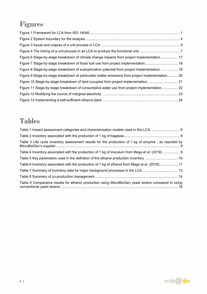
Figures Figure 1 Framework for LCA from ISO 14040. ............................................................................................. 1 Figure 2 System boundary for the analysis. ................................................................................................. 4 Figure 3 Inputs and outputs of a unit process in LCA. ................................................................................. 5 Figure 4 The linking of a unit process in an LCA to produce the functional unit. ......................................... 7 Figure 6 Stage-by-stage breakdown of climate change impacts from project implementation. ................. 17 Figure 7 Stage-by-stage breakdown of fossil fuel use from project implementation. ................................. 18 Figure 8 Stage-by-stage breakdown of eutrophication potential from project implementation. ................. 19 Figure 9 Stage-by-stage breakdown of particulate matter emissions from project implementation........... 20 Figure 10 Stage-by-stage breakdown of land occupied from project implementation. .............................. 21 Figure 11 Stage-by-stage breakdown of consumptive water use from project implementation. ................ 22 Figure 12 Modifying the source of marginal electricity. .............................................................................. 23 Figure 13 Implementing a self-sufficient ethanol plant. .............................................................................. 24

Tables Table 1 Impact assessment categories and characterisation models used in this LCA. ............................. 6 Table 2 Inventory associated with the production of 1 kg of bagasse. ......................................................... 8 Table 3 Life cycle inventory assessment results for the production of 1 kg of enzyme , as reported by MicroBioGen’s supplier. ................................................................................................................................ 9 Table 4 Inventory associated with the production of 1 kg of inoculum from Maga et al. (2019). ................. 9 Table 5 Key parameters used in the definition of the ethanol production inventory. ................................. 10 Table 6 Inventory associated with the production of 1 kg of ethanol from Maga et al. (2019). .................. 11 Table 7 Summary of inventory data for major background processes in the LCA. .................................... 13 Table 8 Summary of co-production management. ..................................................................................... 14 Table 9 Comparative results for ethanol production using MicroBioGen yeast strains compared to using conventional yeast strains. ......................................................................................................................... 16

| 1

1 Introduction

MicroBioGen, in conjunction with its global partner, is developing a ‘fuel and food’ biorefinery concept, which will provide a novel process for converting sugarcane bagasse into ethanol, animal feed and solid fuel, resulting in higher efficiencies than conventional ethanol conversion technologies.

MicroBioGen is completing an A$8 million optimisation project with funding support from the Australian Renewable Energy Agency (ARENA). As a requirement for the funding, a preliminary desktop-based life cycle analysis (LCA) accounting for all factors influencing climate effects (e.g. electricity, transport, waste diversion) is to be completed in order to demonstrate the potential benefits and impacts of the proposal and provide insights into design considerations, in order to optimise the environmental performance of the project.

The study has been undertaken following the requirements of ISO 14044 (International Organization for Standardization 2006a) and in line with the requirements for biofuels and bioenergy assessments established by ARENA (Grant and Bengtsson 2016).

1.1 Life cycle assessment

LCA is a methodology for assessing the full ‘cradle-to-grave’ environmental benefits of products and processes by assessing environmental flows (i.e. impacts) at each stage of the life cycle. LCA aims to include all important environmental impacts for the product system being studied. In doing so, LCA seeks to avoid shifting impacts from one life cycle stage to another or from one environmental impact to another.

The method and guidance for undertaking LCAs of bioenergy products and projects developed by ARENA (Grant and Bengtsson 2016) requires LCAs to be undertaken using the framework, principles and specific requirements defined in both of the international standards, ISO 14040:2006 and ISO 14044:2006 (International Organization for Standardization 2006b). The general structure of the LCA framework is shown in Figure 1.

Figure 1 Framework for LCA from ISO 14040.

The first stage (goal and scope) describes the reasons for the LCA, scenarios, boundaries, indicators and other methodological approaches used. The second stage (inventory analysis) builds a model of the production systems involved in each scenario and describes how each stage of the production process interacts with the environment. The third stage (impact assessment) assesses the inventory data against key indicators to produce an environmental profile of each scenario. The final stage (interpretation) analyses the results and undertakes systematic checks of the assumptions and data to ensure robust results.

2 |

2 Goal

2.1 Reason for the study

This analysis is conducted to meet the requirements of ARENA and provide insights into the environmental impacts and benefits of the optimisation project. As such, the study aims to quantify the environmental impacts and benefits of the fuel and food biorefinery proposed by MicroBioGen and compare it with a ‘business-as-usual’ scenario where ethanol is produced using standard yeast.

This will allow MicroBioGen to ascertain the likelihood of a positive greenhouse gas and energy balance, identify any unintended environmental impacts, and to optimise the overall environmental outcomes of the project.

The aim of the study is focused on comparing the business-as-usual and proposed project scenarios. It is not the intention to assess the environmental effect of producing ethanol in a broader sense. We strongly advise against using the results of this study for that purpose.

2.2 Audience

The primary audience for the study is ARENA and MicroBioGen’s internal team. Audiences may also include external stakeholders, current and future collaborators, investors and prospective investors. Extracts of the information contained herein will be published on MicroBioGen’s website and social media profiles and may from time to time be used in general marketing communications. It will also form part of MicroBioGen’s commitment to ARENA for knowledge sharing to the general public.

| 3

3 Scope

3.1 Functional unit

The international standard on LCA describes the functional unit as defining what is being studied, and states that all analyses should be expressed relative to the functional unit. The definition of the functional unit needs to clearly articulate the function or service that is under investigation. In this study, the two scenarios described below are compared.

1. A ‘proposed project’ scenario where ethanol is produced from bagasse, using a yeast strain produced by MicroBioGen in conjunction with its global partner, and the associated production of yeast-based animal feed and a residual solid waste used as fuel (see Figure 2 for a graphical overview).

2. A ‘business-as-usual’ scenario where ethanol is produced from bagasse, using a standard yeast strain (see Figure 2). Under this scenario, no yeast-based animal feed is produced, but a residual solid waste is still produced.

The functional unit defines the common basis for comparison of alternative options being assessed. In this case, the common basis for comparison between the two scenarios described above is the production of ethanol. Thus, the functional unit is as follows:

“the production of 1 kg of ethanol from waste bagasse arising from sugarcane processing in Queensland.”

The reference flow in an LCA is the amount of the system under study required to deliver the functional unit. In this case, the reference flow is equal to the functional unit.

3.2 System boundary

The system boundary describes the life cycles, stages and processes included in the LCA. In this study, the function was the production of ethanol from bagasse. The project and business-as-usual scenarios are closely aligned, with variations linked to fermentation efficiencies. Both systems are represented in Figure 2 overleaf.

Typically, system boundaries should include everything that is substantially affected by demand for the fuels. This includes extraction and production processes and any additional activities required to make each option functionally equivalent, such as the manufacturing of inputs or the production of heat and electricity. It also includes the effects of co-products along the supply chain.

4 |

Figure 2 System boundary for the analysis.

| 5

3.2.1 Included processes

The LCA includes energy production activities, including bagasse transport and ethanol production in the plant. Infrastructure elements, such as the construction of the plant, were also included, based on generic models rather than primary data collection. Finally, heat produced from natural gas and electricity delivered from the Queensland grid were included, using available models from the AusLCI v1.35 library (ALCAS 2020).

The production of inoculum is included as an alternate path, being only relevant for the business-as-usual scenario. In the case of MicroBioGen, aerobically produced yeast is a by-product of the fermentation process and can be reused, rather than purchased and stocked as dormant yeast. This avoids the need to produce inoculum to bring dormant yeast to optimal conditions. Similarly, the production of feed from excess yeast is only relevant for the proposed project scenario, as no excess yeast is produced in the business-as-usual practice (see Section 4.1 for more details).

3.2.2 Cut-off criteria

The system boundary allowed for the exclusion from the inventory of any flows expected to be less than 1% of any impact category. A cut-off criterion of 1% of mass or energy flows was allowed for with the aim that not more than 5% of flows were excluded from the study. For small flows, estimates were used in preference to exclusion, where possible.

3.3 Flows included in the LCA

Figure 3 shows the characterisation of flows included in the LCA. These included flows to and from the environment as well as flows to and from other technical processes (the technosphere).

Figure 3 Inputs and outputs of a unit process in LCA.

6 |

3.4 Environmental impact categories

Table 1 describes each of the indicators chosen for LCA and the source of the characterisation factors.

Table 1 Impact assessment categories and characterisation models used in this LCA.

INDICATOR DESCRIPTION CHARACTERISATION MODEL Climate change Measured in kg CO2 eq.

This is governed by the increased concentrations of greenhouse gases in the atmosphere, that is, gases that trap heat and lead to higher global temperatures. The principal anthropogenic greenhouse gases are carbon dioxide, methane and nitrous oxide.

IPCC Global warming potential model based on 100-year timeframe (IPCC 2013).

Fossil energy use Measured in MJ lower heating value. It includes all energy resources extracted and used in any way. It does not include renewable energy, energy from waste or nuclear energy.

All fossil energy carriers based on lower heating values.

Eutrophication Measured in g PO4-3 eq. Algal growth from nutrient enrichment in freshwater and marine environments. Emission of nitrogen and phosphorus contribute with the model being based on the redfield ratio.

CML method based on redfield ratio (Institute of Environmental Sciences (CML) 2016).

Particulate matter Measured in g PM2.5 eq. This impact category looks at the health impacts from particulate matter for PM10 and PM2.5. This is one of the most dominant immediate risks to human health as identified in the global burden of disease.

IMPACT World+ method, based on Humbert et al. (2011) and Bulle et al. (2019).

Land use Measured in ha of land occupied per year. This indicator measures the area of land occupied by the system.

All land use based on area occupied.

Consumptive water use

Measured in litres of water. This indicator measures the net volume of water consumed by the system under assessment.

Net water use based on extraction minus release.

| 7

4 Inventory analysis

Inventory analysis is the stage of the LCA in which the system being studied is broken up into unit processes. The unit processes fall within the foreground or background of the model, as defined below:

• Model foreground includes unit processes for which specific data are collected for the study, refer to as foreground processes. The model foreground may also include secondary data from published papers and modified background processes from LCA databases.

• Model background includes unit processes for which data are typically sourced from pre-existing databases. The background data are either less important to the study outcomes or are already well-characterised in the existing data sets and therefore do not warrant specific modelling. In some instances, background unit processes may be modified to better reflect the conditions of the study. (e.g. to reflect greenhouse gas intensity of local electricity supply). In that case, they become part of the foreground

Figure 4 shows how unit processes were linked to create a system that produces the functional unit of the study. The following sections outline the sources of the background and foreground inventory data.

Figure 4 The linking of a unit process in an LCA to produce the functional unit.

8 |

4.1 Foreground data

A summary of the data sources and assumptions for the foreground data are described in this section.

• Inputs associated with bagasse production are reported in Table 2. • Enzymes were modelled based on impact assessment results provided by MicroBioGen enzyme’s

supplier, as reported in Table 3. • Inputs required to produce inoculum are shown in Table 4. • Key parameters influencing the ethanol production inventory are listed in Table 5. • Ethanol production, for both the business-as-usual and project scenarios, was modelled as reported

in Table 6.

The issue of allocation of flows is reported in Section 4.3. This applies to key aspects of the model, namely the input of bagasse (a co-product of the sugar milling process), and the output of a yeast-based animal feed and residual solid waste used for energy generation.

Table 2 Inventory associated with the production of 1 kg of bagasse.

DATA UNIT VALUE COMMENT Transport kg.km 5 As reported by MicroBioGen, the ethanol plant is likely to be

located in close proximity to a sugar mill, to limit double handling and transport costs.

Avoided electricity export

kWh 0.065 In FY12, the sugar industry exported 488 GWh of electricity to the Queensland grid, produced from the combustion of bagasse at the sugar mills (Department of Infrastructure and Regional Development 2015). The total bagasse production for the same year was reported as 7.5 million tonnes (Department of Infrastructure and Regional Development 2015). These factors allow to estimate the electricity exported to the grid per kg of bagasse produced.

Avoided bagasse combustion

Assuming emissions occur in low population areas. This is particularly relevant for the Particulate Matter impact indicator. Emissions in high population areas are assumed to have more significant effects on human health than in low population areas. This is reflected in the definition of the impact assessment factors, where PM2.5 emitted in high population area has an emission factor of 3.33 while it is 0.35 in low population areas.

− Carbon monoxide g 2.61 Assuming the use of a wet scrubber. Emissions representative of a boiler, as reported in NPI (2011).

− Nitrogen oxides g 0.76 Assuming the use of a wet scrubber. Emissions representative of a boiler, as reported in NPI (2011).

− Particulate matter, >2.5 µm, <10 µm

g 0.22 Assuming the use of a wet scrubber. Emissions representative of a boiler, as reported in NPI (2011).

− Particulate matter <2.5 µm

g 0.126 Assuming the use of a wet scrubber. Emissions representative of a boiler, as reported in NPI (2011).

− Polycyclic aromatic hydrocarbons

g 5e-4 Assuming the use of a wet scrubber. Emissions representative of a boiler, as reported in NPI (2011).

− Sulphur dioxide g 0.25 Assuming the use of a wet scrubber. Emissions representative of a boiler, as reported in NPI (2011).

− Polychlorinated dioxins and furans

g 4.75e-

10 Assuming the use of a wet scrubber. Emissions representative of a boiler, as reported in NPI (2011).

MicroBioGen reported that enzymes would be externally supplied rather than produced on-site, with a major enzyme manufacturer being the expected supplier. MicroBioGen’s international partner provided life cycle inventory assessment results for the six indicators considered in this study, using the same impact

| 9

assessment methods, the result of which is reported in the table below. These values are used to represent the production of enzymes in the model.

Table 3 Life cycle inventory assessment results for the production of 1 kg of enzyme , as reported by MicroBioGen’s supplier.

IMPACT CATEGORY UNIT VALUE Climate change kg CO2 eq 2.25

Fossil energy use MJ 27.1

Eutrophication kg PO43- eq 0.0116

Particulate matter kg PM2.5 eq 0.00153

Land use m2.year-1 0.556

Consumptive water use m3 0.0301

During the inoculum development stage, a dormant stock culture of microorganisms is raised to a state at which can be used to inoculate a hydrolysed batch of bagasse and start the fermentation process (Webb and Kamat 1993). Typically, dormant stocks of yeast are purchased by ethanol plant, and inoculum development happens on-site. This production system is used to represent the business-as-usual scenario. At the end of the ethanol production chain, the yeast that is left from the fermentation is found in the liquid waste arising from the process, the vinasse. Typically, yeasts are inhibited by the mix of chemical found in vinasse, which is why inoculum must be continuously produced to support the production of ethanol. The model used to represent inoculum development is based on the literature (Maga et al. 2019), and subsequently regionalised to be representative of Australian production.

In the case of MicroBioGen, the yeast is able to survive and grow on by-products of the fermentation such as xylose and can therefore be left to grow on the vinasse and subsequently reused. The surplus yeast from this step can then be separated to produce animal feed.

Table 4 Inventory associated with the production of 1 kg of inoculum from Maga et al. (2019).

DATA UNIT VALUE DATA UNIT VALUE Input Output

Diammonium phosphate kg 0.221 Carbon dioxide, to air kg 0.63

Molasses kg 1.51 Wastewater litres 20

Liquid oxygen kg 0.462

Water kg 19.4

Electricity kWh 0.348

The inventory developed to represent ethanol production is built using from data published in the report documenting the ecoinvent inventory for ethanol produced from wood chips an (Jungbluth et al. 2007), modified with data from a recent scientific publication focusing on second generation ethanol production from bagasse in Brazil (Maga et al. 2019), and a series of critical parameters provided by MicroBioGen.

A summary of key parameters used throughout the inventory is provided in Table 5.

10 |

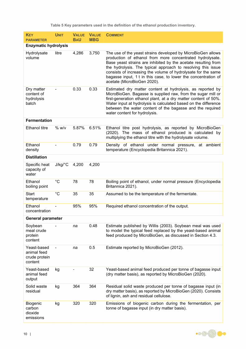
Table 5 Key parameters used in the definition of the ethanol production inventory.

KEY PARAMETER

UNIT VALUE BAU

VALUE MBG

COMMENT

Enzymatic hydrolysis

Hydrolysate volume

litre 4,286 3,750 The use of the yeast strains developed by MicroBioGen allows production of ethanol from more concentrated hydrolysate. Base yeast strains are inhibited by the acetate resulting from the hydrolysis. The typical approach to resolving this issue consists of increasing the volume of hydrolysate for the same bagasse input, 1 t in this case, to lower the concentration of acetate (MicroBioGen 2020).

Dry matter content of hydrolysis batch

- 0.33 0.33 Estimated dry matter content at hydrolysis, as reported by MicroBioGen. Bagasse is supplied raw, from the sugar mill or first-generation ethanol plant, at a dry matter content of 50%. Water input at hydrolysis is calculated based on the difference between the water content of the bagasse and the required water content for hydrolysis.

Fermentation

Ethanol titre % w/v 5.87% 6.51% Ethanol titre post hydrolysis, as reported by MicroBioGen (2020). The mass of ethanol produced is calculated by multiplying the ethanol titre with the hydrolysate volume.

Ethanol density

- 0.79 0.79 Density of ethanol under normal pressure, at ambient temperature (Encyclopedia Britannica 2021).

Distillation

Specific heat capacity of water

J/kg/°C 4,200 4,200

Ethanol boiling point

°C 78 78 Boiling point of ethanol, under normal pressure (Encyclopedia Britannica 2021).

Start temperature

°C 35 35 Assumed to be the temperature of the fermentate.

Ethanol concentration

- 95% 95% Required ethanol concentration of the output.

General parameter

Soybean meal crude protein content

- na 0.48 Estimate published by Willis (2003). Soybean meal was used to model the typical feed replaced by the yeast-based animal feed produced by MicroBioGen, as discussed in Section 4.3.

Yeast-based animal feed crude protein content

- na 0.5 Estimate reported by MicroBioGen (2012).

Yeast-based animal feed output

kg - 32 Yeast-based animal feed produced per tonne of bagasse input (dry matter basis), as reported by MicroBioGen (2020).

Solid waste residual

kg 364 364 Residual solid waste produced per tonne of bagasse input (in dry matter basis), as reported by MicroBioGen (2020). Consists of lignin, ash and residual cellulose.

Biogenic carbon dioxide emissions

kg 320 320 Emissions of biogenic carbon during the fermentation, per tonne of bagasse input (in dry matter basis).

| 11

A key aspect of the analysis is the process yield. MicroBioGen shared the ethanol titre of the fermentate, and the hydrolysate volume for a bagasse input of 1 tonne. This allows us to estimate the mass of bagasse required to produce 1 kg of ethanol. The mass of ethanol produced is calculated by multiplying the ethanol titre with the hydrolysate volume. Based on the key parameters provided by MicroBioGen, we estimated that 1 tonne of bagasse will produce 244 kg of ethanol using the MicroBioGen yeast, while a base strain will produce 252 kg. Although the ethanol yield is lower, the yeast strains developed by MicroBioGen are resistant to acetate, which is a by-product of hydrolysis and tends to inhibit typical yeast strains. Thus, MicroBioGen can process a similar volume of bagasse in a smaller hydrolysate volume. At the distillation stage, it means that a lower volume of liquid needs to be heated to distil the ethanol, leading to improved energy efficiencies. In addition, MicroBioGen is able to produce a yeast-based animal feed from the excess yeast separated post-fermentation, which would die off in the business-as-usual scenario.

The heat requirement at distillation was estimated using the equation:

𝐸𝑑𝑖𝑠𝑡𝑖𝑙𝑙𝑎𝑡𝑖𝑜𝑛 = 𝐶𝑤𝑎𝑡𝑒𝑟 × 𝑉ℎ𝑦𝑑𝑟𝑜𝑙𝑦𝑠𝑎𝑡𝑒 × (𝐵𝑃𝑒𝑡ℎ𝑎𝑛𝑜𝑙 − 𝑇𝑓𝑒𝑟𝑚𝑒𝑛𝑡𝑎𝑡𝑒) (1)

Where 𝐸𝑑𝑖𝑠𝑡𝑖𝑙𝑙𝑎𝑡𝑖𝑜𝑛 is the heat requirements at distillation, in joules per tonne of bagasse, 𝐶𝑤𝑎𝑡𝑒𝑟 is the amount of energy required to raise 1 kg of water by 1°C, 𝑉ℎ𝑦𝑑𝑟𝑜𝑙𝑦𝑠𝑎𝑡𝑒 is the volume of hydrolysate to be distilled (assuming a density of 1), 𝐵𝑃𝑒𝑡ℎ𝑎𝑛𝑜𝑙 the boiling point of ethanol and 𝑇𝑓𝑒𝑟𝑚𝑒𝑛𝑡𝑎𝑡𝑒 the assumed temperature of the solution post-fermentation.

Table 6 Inventory associated with the production of 1 kg of ethanol from Maga et al. (2019).

DATA UNIT VALUE BAU

VALUE MBG

COMMENT

INPUTS

Pre-treatment

Bagasse (wet mass)

kg 7.95 8.19 Calculated as 1,000 kg bagasse (in dry matter basis) divided by the mass of ethanol produced, assuming 50% water content in bagasse.

Sulfuric acid kg 0.85 0.088 Reported in ecoinvent as 0.012 kg per 0.555 kg dried wood chips, pro-rated to the bagasse inputs (dry matter basis).

Quicklime kg 0.033 0.034 Reported in ecoinvent as 0.0046 kg per 0.555 kg dried wood chips, pro-rated to the bagasse inputs (dry matter basis).

Organic chemicals

kg 2.5e-4 2.5e-4 Reported in ecoinvent as 3.45e-5 per 0.555 kg dried wood chips, pro-rated to the bagasse inputs (dry matter basis).

Electricity kWh 0.096 0.099 Electricity reported in ecoinvent as 13.5 kWh per 0.555 kg dried wood chips, pro-rated to the bagasse inputs (dry matter basis).

Heat MJ 7.06 7.28 Heat reported in ecoinvent as 987 MJ per 0.555 kg dried wood chips, pro-rated to the bagasse inputs (dry matter basis).

Enzymatic hydrolysis

Enzyme solution

kg 0.063 0.063 Enzyme will be produced by leading enzyme manufacturer with an Australian manufacturing site. Transport was estimated as 250 km by road. Input estimated based on information provided by MicroBioGen’s enzyme supplier.

Water litres 4.1 4.22 Water volume required to achieve 33% dry matter content in the hydrolysate.

Electricity kWh 0.43 0.44 Based on a value of 10,431 kWh for 127 t bagasse (50% DM) and 40 t trash (15% DM) (Maga et al. 2019).

12 |

Cooling water litres 49.9 51.5 Based on a value of 1,222 m3 for 127 t bagasse (50% DM) and 40 t trash (15% DM) (Maga et al. 2019).

Fermentation

Inoculum kg 0.19 - Based on a value of 4.7 kg for 127 t bagasse (50% DM) and 40 t trash (15% DM) (Maga et al. 2019).

Water litres 7.7 5.78 Assumed to be the difference between the volume of hydrolysate reported in Table 5, and the volume of ethanol produced (calculated as the mass of ethanol divided by the density).

Electricity kWh 0.18 0.19 Based on a value of 4,497 kWh for 127 t bagasse (50% DM) and 40 t trash (15% DM) (Maga et al. 2019).

Cooling water litres 65.4 67.4 Based on a value of 1,600 m3 for 127 t bagasse (50% DM) and 40 t trash (15% DM) (Maga et al. 2019).

Distillation

Heat MJ 3.08 2.77 Estimated based on the amount of energy required to heat the fermentate above the boiling point of ethanol, but under the boiling point of water (for the purpose of the analysis, we used 85°C).

Cooling water litres 441 454 Based on a value of 10,789 m3 for 127 t bagasse (50% DM) and 40 t trash (15% DM) (Maga et al. 2019).

Infrastructure

Ethanol fermentation plant

unit 3.7e-10 3.7e-10 The model used is sourced from ecoinvent and represents a 90,000 t production capacity plant. The plant lifetime is assumed to be 30 years.

OUTPUT

Ethanol (95% concentration)

kg 1 1

Yeast-based animal feed

kg - 0.19 Based on information reported by MicroBioGen, estimating 32 kg of yeast produced from 1 t of bagasse.

Solid residue (lignin, ash and cellulose)

kg 1.45 1.49 Based on information reported by MicroBioGen, estimating 364 kg of residue produced from 1 t of bagasse. It is assumed to displace the production of electricity from coal in Queensland and is modelled to be equal to bagasse in terms of emissions and avoided electricity production (adjusting for the moisture content).

Wastewater litres 15.9 14 All process water entering the system is assumed to be treated in wastewater treatment plants. The inoculum is also accounted here when relevant.

Water release to nature

litres 556 573 All cooling water entering the system is assumed to be released into the environment (Maga et al. 2019).

Biogenic carbon dioxide emissions

kg 1.27 1.31 Emissions associated with yeast respiration during fermentation, based on data reported by MicroBioGen. Note that this emission is assumed to be neutral on the Climate Change indicator, but is reported due to its significance on the mass balance of the process.

| 13

4.2 Background data

While hundreds of background processes contributed to the LCA, the most important processes were those that affected the results or those that were modified from the original source to better represent an input to this LCA. These background processes, data sources and modifications are summarised in Table 7.

Table 7 Summary of inventory data for major background processes in the LCA.

PROCESS/EMISSION SOURCE COMMENT Electricity, Queensland (ALCAS 2020) Unmodified AusLCI v1.35 inventory Heat from natural gas, Queensland

(ALCAS 2020) Unmodified AusLCI v1.35 inventory

Ethanol fermentation plant

(ALCAS 2020) Modified ecoinvent inventory integrated into AusLCI v1.35

Sulfuric acid (ALCAS 2020) Modified ecoinvent inventory integrated into AusLCI v1.35

Quicklime (ALCAS 2020) Modified ecoinvent inventory integrated into AusLCI v1.35

Organic chemical (ALCAS 2020) Modified ecoinvent inventory integrated into AusLCI v1.35

Road transport (ALCAS 2020) Unmodified AusLCI v1.35 inventory Sea transport (ALCAS 2020) Unmodified AusLCI v1.35 inventory Process water, Australia (ALCAS 2020) Unmodified AusLCI v1.35 inventory Wastewater treatment, Queensland

(ALCAS 2020) Unmodified AusLCI v1.35 inventory

Diammonium phosphate (ALCAS 2020) Modified ecoinvent inventory integrated into AusLCI v1.35

Molasses (ALCAS 2020) Unmodified AusLCI v1.35 inventory Liquid oxygen, Australia (ALCAS 2020) Modified ecoinvent inventory integrated into AusLCI

v1.35 Soybean meal (Weidema et al. 2018) Unmodified ecoinvent v3.5 inventory (cut-off),

representative of the global market

4.3 Multi-functionality

Multi-functionality occurs when a single process or group of processes produces more than one usable output, or ‘co-product’. ISO defines a co-product1 as “any of two or more products coming from the same unit process or product system”. A product is any good or service, so by definition it has some value for the user. This is distinct from a ‘waste’, which ISO defines as “substances or objects which the holder intends or is required to dispose of”, and therefore has no value to the user.

As LCA identifies the impacts associated with a discrete product or system, it is necessary to separate the impact of co-products arising from multifunction processes.

Many co-products are used and produced when making biofuels. In fact, the drive to produce fuels from non-food sources and to minimise competition with food and feed production, encourages fuel producers to use waste and co-products from other sectors in their production.

Processes presenting an issue of multi-functionality were handled by expanding the boundary of the system. This is graphically represented in Figure 2. A summary of the approach for each co-product is presented in Table 8.

1 While there are subtle differences that can be found between by-products and co-products in LCA there is no distinction in this study between a co-product and a by-product.

14 |

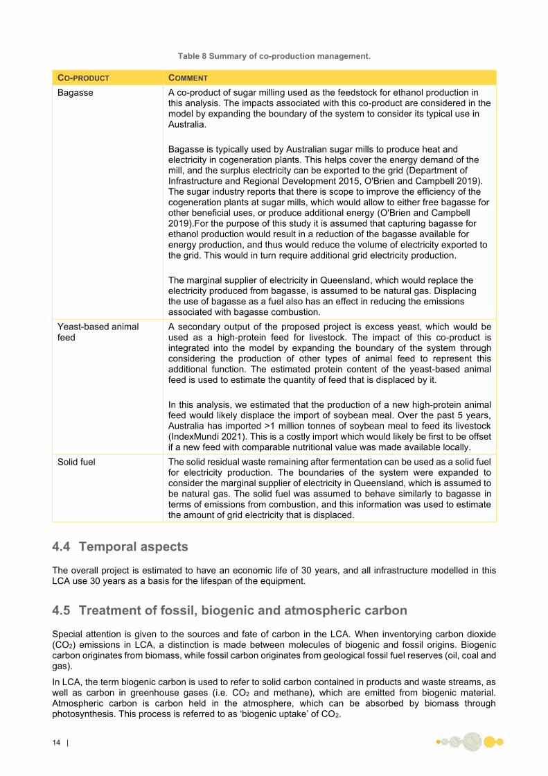
Table 8 Summary of co-production management.

CO-PRODUCT COMMENT Bagasse A co-product of sugar milling used as the feedstock for ethanol production in

this analysis. The impacts associated with this co-product are considered in the model by expanding the boundary of the system to consider its typical use in Australia. Bagasse is typically used by Australian sugar mills to produce heat and electricity in cogeneration plants. This helps cover the energy demand of the mill, and the surplus electricity can be exported to the grid (Department of Infrastructure and Regional Development 2015, O'Brien and Campbell 2019). The sugar industry reports that there is scope to improve the efficiency of the cogeneration plants at sugar mills, which would allow to either free bagasse for other beneficial uses, or produce additional energy (O'Brien and Campbell 2019).For the purpose of this study it is assumed that capturing bagasse for ethanol production would result in a reduction of the bagasse available for energy production, and thus would reduce the volume of electricity exported to the grid. This would in turn require additional grid electricity production. The marginal supplier of electricity in Queensland, which would replace the electricity produced from bagasse, is assumed to be natural gas. Displacing the use of bagasse as a fuel also has an effect in reducing the emissions associated with bagasse combustion.

Yeast-based animal feed

A secondary output of the proposed project is excess yeast, which would be used as a high-protein feed for livestock. The impact of this co-product is integrated into the model by expanding the boundary of the system through considering the production of other types of animal feed to represent this additional function. The estimated protein content of the yeast-based animal feed is used to estimate the quantity of feed that is displaced by it. In this analysis, we estimated that the production of a new high-protein animal feed would likely displace the import of soybean meal. Over the past 5 years, Australia has imported >1 million tonnes of soybean meal to feed its livestock (IndexMundi 2021). This is a costly import which would likely be first to be offset if a new feed with comparable nutritional value was made available locally.

Solid fuel The solid residual waste remaining after fermentation can be used as a solid fuel for electricity production. The boundaries of the system were expanded to consider the marginal supplier of electricity in Queensland, which is assumed to be natural gas. The solid fuel was assumed to behave similarly to bagasse in terms of emissions from combustion, and this information was used to estimate the amount of grid electricity that is displaced.

4.4 Temporal aspects

The overall project is estimated to have an economic life of 30 years, and all infrastructure modelled in this LCA use 30 years as a basis for the lifespan of the equipment.

4.5 Treatment of fossil, biogenic and atmospheric carbon

Special attention is given to the sources and fate of carbon in the LCA. When inventorying carbon dioxide (CO2) emissions in LCA, a distinction is made between molecules of biogenic and fossil origins. Biogenic carbon originates from biomass, while fossil carbon originates from geological fossil fuel reserves (oil, coal and gas).

In LCA, the term biogenic carbon is used to refer to solid carbon contained in products and waste streams, as well as carbon in greenhouse gases (i.e. CO2 and methane), which are emitted from biogenic material. Atmospheric carbon is carbon held in the atmosphere, which can be absorbed by biomass through photosynthesis. This process is referred to as ‘biogenic uptake’ of CO2.

| 15

In this analysis, bagasse is used to produce ethanol. A significant proportion of the original biomass is not converted to ethanol and used as a fuel. Data from AusLCI (ALCAS 2020) suggest that bagasse has a carbon content of 0.5 (in dry matter basis), which allows us to estimate that the carbon equivalent of 1.83 kg CO2 was sequestered per kilogram of plant biomass. The sequestered CO2 is assumed to be released either during the combustion of the residual waste or as a by-product of the fermentation process. As such, the sequestration and emissions of biogenic carbon dioxide are modelled as being neutral on the climate change indicator.

4.6 Land use change (LUC)

In this project, there is no dedicated production system used to supply feedstock to the ethanol plant. Thus, land use change is not expected to have any impact on the results of this analysis.

4.7 Reference system

The reference system utilises conventional yeast strains to produce ethanol using a similar production system to the proposed project. It requires the development of inoculum from dormant yeast, while the proposed project does not. In both cases, the residual solid waste output is used to produce electricity, displacing conventional energy sources. To account for the production of yeast-based animal feed in the proposed project, the system boundaries have been expanded to include the production of an equivalent volume of conventional animal feed (assuming soybean meal).

16 |

5 Impact assessment

5.1 Impact assessment indicators and characterisation models

The impact assessment stage relates the inventory flows to the indicators chosen for the LCA. This is done by classifying which flows relate to which impact indicator and then selecting a characterisation model that quantifies the relationship of each inventory type to the indicator in question. For example, flows of carbon dioxide and methane are both known to contribute to the climate change indicator. The characterisation model chosen for the study was the 2013 Intergovernmental Panel on Climate Change 100-year Global Warming Potential model. This uses carbon dioxide as the reference substance with a characterisation factor of 1 and methane with a characterisation factor of 25 carbon dioxide equivalents. An equivalent approach is applied across all indicators. The calculation of the indicator results is the summation of all inventory flows multiplied by their relevant characterisation factors. This step is referred to as characterisation. The results are in equivalent units, such as kg CO2 eq., for each indicator.

Note: a positive value denotes an impact, while a negative value can be interpreted as a reduction of the impacts.

5.2 Results

The high-level results of the analysis are presented in Table 9 below. Comparative results show the difference between the impacts of the proposed project and the business-as-usual scenarios. A detailed analysis of each indicator, including an explanation of the underlying trends, is reported in Sections 6.1 to 0.

Table 9 Comparative results for ethanol production using MicroBioGen yeast strains compared to using conventional yeast strains.

CLIMATE CHANGE

FOSSIL ENERGY USE

PARTICULATE MATTER EUTROPHICATION CONSUMPTIVE

WATER USE LAND USE

kg CO2 eq. MJ NCV g PM2.5 t PO4-3 eq. L m2.year-1

Proposed project 1.32 22.2 -0.02 0.83 4.6 -2.32

Business-as-usual 1.85 25.0 0.25 1.66 18.8 1.66

Comparative results -29% -11% -108% -50% -75% -240%

| 17

6 Interpretation

The interpretation step examines the results through a series of steps used to ensure that the conclusions drawn from the LCA are robust and well supported by the data and selected impact modelling. A contribution analysis is conducted to identify the hotspots in the system analysed for all six of the considered indicators.

6.1 Contribution analysis

6.1.1 Climate change

Impacts associated with the operation of the proposed project are partly offset by the production of animal feed from excess yeast production and avoided electricity production through the solid fuel output (Figure 5).

Displacing bagasse from its conventional use in sugar mills for energy production and export a significant driver of emissions in the model. The amount of additional electricity that needs to be produced to cover the losses associated with capturing bagasse for ethanol production is close to the total electricity requirement of producing ethanol.

Emissions at pre-processing are driven by the heat requirements estimated for the pre-processing step, while emissions at hydrolysis are strongly linked to the estimated electricity requirements, as well as enzymes input. The benefits associated with the avoided animal feed are notably driven by the avoided emissions associated with land use change for the production of soybeans. Apart from the production of a yeast-based animal feed, the proposed project benefits from not requiring external input of inoculum to start the fermentation process, notably due to the energy and nutrients requirements reported in Table 4.

Figure 5 Stage-by-stage breakdown of climate change impacts from project implementation.

-0.4

-0.2

0.0

0.2

0.4

0.6

0.8

Bagasse(displaced fromenergy prod.)

Pre-processing Hydrolysis Fermentation Ethanoldistillation

Infrastructure Residual wastecombustion

(displacing conv.electricity)

Yeast-basedanimal feed

(displacing conv.feed)

kg C

O2e

/ kg

eth

anol

18 |

6.1.2 Fossil fuel use

The way fossil fuel use is distributed throughout the system is closely aligned with what has been reported for climate change. Here, we can observe that fossil fuel use from pre-processing and hydrolysis is significant (Figure 6). Pre-processing requires a significant input of heat, provided by natural gas. Heat production from natural gas has a much lower emission profile than electricity from the grid, which explains the variation. On the other hand, the hydrolysis stage requires a significant input of electricity.

Another significant difference with the climate change results is the impact of avoided animal feed, which does not play a significant role when comparing the two scenarios against the fossil fuel use indicator. This is because the impacts of the avoiding conventional animal feed on climate change are mostly related to issues of land use and land use change, which plays not part in the fossil fuel use indicator.

Figure 6 Stage-by-stage breakdown of fossil fuel use from project implementation.

-4

-2

0

2

4

6

8

10







MJ

/ kg

etha

nol

| 19

6.1.3 Eutrophication

Eutrophication impacts result from the emission of pollutants, which eventually end up in a water body. These molecules are generally nitrogen or phosphorous based, and they set off a chain reaction that starts with significant algal growth and ends with the depletion of oxygen resources in the water and a significant decline in wildlife population as a consequence.

Impacts against this indicator are offset in part by the displacement of soybean meal through the production of yeast-based animal feed, as is apparent in Figure 7. Soy production involves the application of phosphorous fertiliser, which contributes to eutrophication. The main drivers for eutrophication impacts are linked to the use of electricity throughout the ethanol production process, as well as emissions associated with wastewater treatment during the process.

One significant benefit of the proposed project over the business-as-usual scenario is avoiding the need to develop an inoculum. The production of inoculum as reported in Table 4 requires the use of molasses, which drives the eutrophication impacts through its link to sugar cane production.

Figure 7 Stage-by-stage breakdown of eutrophication potential from project implementation.

-0.6

-0.4

-0.2

0.0

0.2

0.4

0.6

0.8

1.0

1.2







kg P

O43-

eq/ k

g et

hano

l

20 |

6.1.4 Particulate matter

The exposure to particulate matter has a direct effect on human health, being a major cause of respiratory disease globally. Although overall exposure of the population is low in regional Australia, the exposure of the population can still have significant health consequences.

The trend regarding emissions of particulate matter is closely linked to combustion processes. Here, it appears that displacing bagasse from energy production towards ethanol production has a beneficial impact on particulate matter (Figure 8). Emissions from biomass combustion occur later when the solid fuel resulting from ethanol production is used to produce energy and displace electricity.

Avoiding the production of conventional animal feed, in this case of soybean meal, has a significant beneficial impact on the results. Emissions of particulate matter from the global soybean supply chain are mostly linked to land use change issues associated with the production of soybean.

Avoiding the development of inoculum in the proposed project reduces the impacts of fermentation significantly. As reported in Table 4, the inoculum requires an input of diammonium phosphoate, which drives the impacts on particulate matter through emissions in its supply chain

Figure 8 Stage-by-stage breakdown of particulate matter emissions from project implementation.

-0.30

-0.25

-0.20

-0.15

-0.10

-0.05

0.00

0.05

0.10

0.15

0.20



Infrastructure Residual wastecombustion(displacing

conv. electricity)

Yeast-basedanimal feed(displacingconv. feed)

g PM

2.5

/ kg

etha

nol

| 21

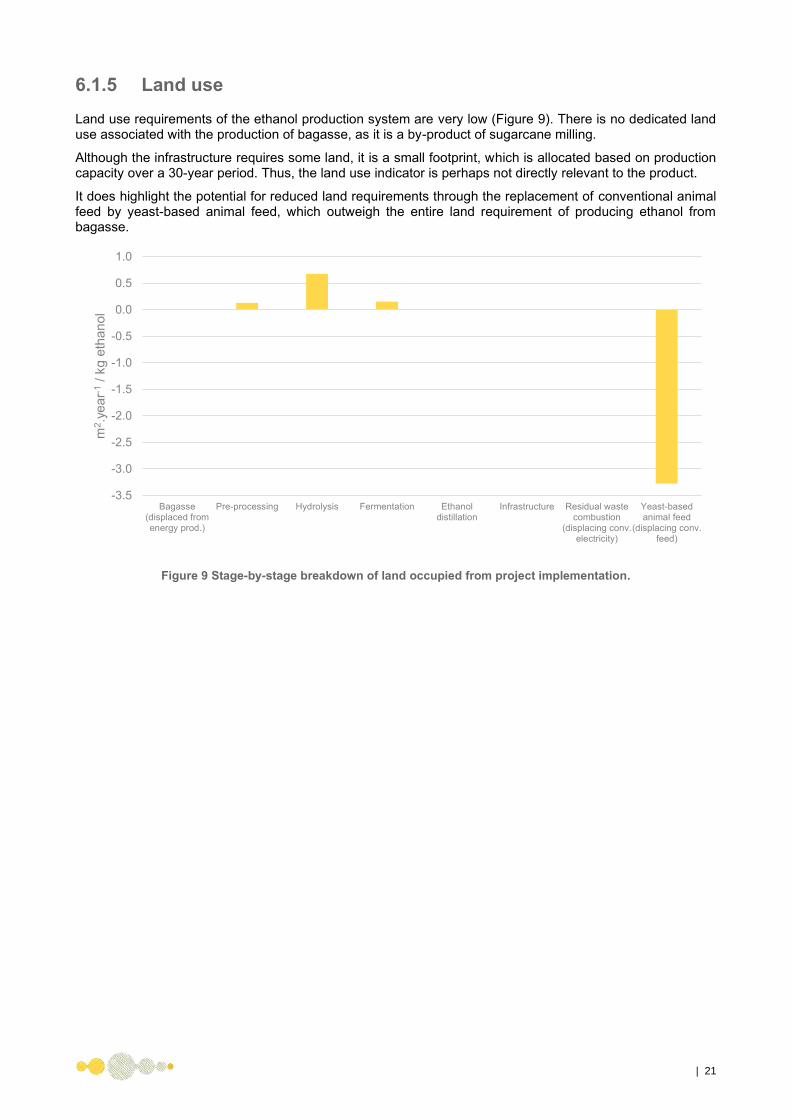
6.1.5 Land use

Land use requirements of the ethanol production system are very low (Figure 9). There is no dedicated land use associated with the production of bagasse, as it is a by-product of sugarcane milling.

Although the infrastructure requires some land, it is a small footprint, which is allocated based on production capacity over a 30-year period. Thus, the land use indicator is perhaps not directly relevant to the product.

It does highlight the potential for reduced land requirements through the replacement of conventional animal feed by yeast-based animal feed, which outweigh the entire land requirement of producing ethanol from bagasse.

Figure 9 Stage-by-stage breakdown of land occupied from project implementation.

-3.5

-3.0

-2.5

-2.0

-1.5

-1.0

-0.5

0.0

0.5

1.0







m2 .y

ear-1

/ kg

etha

nol

22 |

6.1.6 Consumptive water use

The water requirement associated with producing ethanol is relatively high, at ~10 litre process water/kg ethanol (Figure 10), though it is mitigated by the high water content of the bagasse feedstock. The hydrolysis stage is where most process water is required. A significant volume of cooling water is used throughout the process, though it is assumed to be released into the environment, and thus is considered neutral. The proposed project allows the production of ethanol in a more concentrated hydrolysate, which allows a reduction in water requirements.

Here, the fermentation process is reported as net negative, as the water inputs throughout the process are modelled as being treated and released in the environment at the end of the fermentation process.

Figure 10 Stage-by-stage breakdown of consumptive water use from project implementation.

-10

-8

-6

-4

-2

0

2

4

6

8

10







litre

/ kg

eth

anol

| 23

6.2 Sensitivity analysis

Specific aspects of the analysis rely on key assumptions which are critical to the results. Two significant points where identified during this analysis, and are reviewed in the following subsections:

1. the definition of the marginal supplier of electricity; 2. the export of residual solid waste off-site rather than its use to power the ethanol plant.

6.2.1 Marginal supplier of electricity

The food and fuel biorefinery planned by MicroBioGen, if successfully built, would start producing in approximately five years, and would be productive for several decades after that. It is of course impossible to know with certainty what the marginal supplier of electricity will be decades from now, though we can rely on trends and current policies to make an educated guess.

The three principal candidates are coal, natural gas, and renewable electricity. An analysis was conducted to assess the impacts of modifying our assumption regarding the marginal supplier of electricity. The results of the analysis are shown in Figure 11, showing natural gas to be a middle ground between coal and renewable energy. The use of renewable energy as the marginal supplier would reduce the impacts on climate change by 10%, while they would increase by 13% if coal was the marginal supplier.

This suggests that using natural gas as the marginal supplier is a balanced assumption and is appropriate for the purpose of this analysis. It should be noted that this assumption used is applied for both the business-as-usual and proposed project, and as such would not impact the result of the assessment, which is strictly to compare the two scenarios.

Figure 11 Modifying the source of marginal electricity.

-0.5

0.0

0.5

1.0

1.5

2.0

kg C

O2e

/ kg

eth

anol

Proposed project - coal Proposed project - Natural gas Proposed project - renewable

24 |

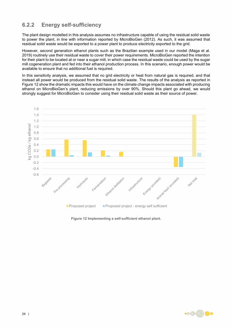
6.2.2 Energy self-sufficiency

The plant design modelled in this analysis assumes no infrastructure capable of using the residual solid waste to power the plant, in line with information reported by MicroBioGen (2012). As such, it was assumed that residual solid waste would be exported to a power plant to produce electricity exported to the grid.

However, second generation ethanol plants such as the Brazilian example used in our model (Maga et al. 2019) routinely use their residual waste to cover their power requirements. MicroBioGen reported the intention for their plant to be located at or near a sugar mill, in which case the residual waste could be used by the sugar mill cogeneration plant and fed into their ethanol production process. In this scenario, enough power would be available to ensure that no additional fuel is required.

In this sensitivity analysis, we assumed that no grid electricity or heat from natural gas is required, and that instead all power would be produced from the residual solid waste. The results of the analysis as reported in Figure 12 show the dramatic impacts this would have on the climate change impacts associated with producing ethanol on MicroBioGen’s plant, reducing emissions by over 90%. Should this plant go ahead, we would strongly suggest for MicroBioGen to consider using their residual solid waste as their source of power.

Figure 12 Implementing a self-sufficient ethanol plant.

-0.6

-0.4

-0.2

0.0

0.2

0.4

0.6

0.8

1.0

1.2

1.4

1.6

kg C

O2e

/ kg

eth

anol

Proposed project Proposed project - energy self sufficient

| 25

7 Discussion and conclusions

Based on the data available and assumptions applied throughout this LCA, the proposed project appears to be beneficial on all indicators considered. This is linked to:

• avoiding the need to rely on the development of inoculum in the fermentation stage • allowing the production of ethanol from a more concentrated hydrolysate using MicroBioGen yeast

strains, thus reducing distillation impacts • the production of an animal feed which displaces conventional feed such as soybean meal

This study, like any LCA, has limitations – some of which have already been discussed throughout the report. It is worth pointing out that an LCA is a model, and as such it relies on assumptions and approximations. The ability to use these assumptions and approximations is what enables the completion of an LCA.

Apart from some key parameters shared by MicroBioGen, the ethanol production model is based on data reported in Jungbluth et al. (2007), which itself largely relies on published data from the 2000’s. Aspects of the model are based on a more recent study published by Maga et al. (2019). This is appropriate for the purpose of this study, which is to compare using a strain of yeast produced by MicroBioGen with the use of a conventional yeast strain with the most uncertain parameters being common to both. It would however be inappropriate to take the results of this analysis outside of this context, and assume they broadly represented the environmental impacts associated with ethanol production.

There are several aspects of the proposed project which are significant to the final results. The first one is the energy and water requirements associated with ethanol production, which are based on literature data from overseas, and are significant contributors to several indicators. The second is avoiding the need for an inoculum to activate the yeasts, as excess yeast is produced by the process and can be reused later. The choice of displaced animal feed also plays an important role. Soybean meal appears to be an appropriate choice, based on the level of import and its crude protein content which align with the yeast-based animal feed that would be produced. The use of the global soybean supply chain links back to Brazilian production, which is modelled as includes direct land use change in its production. These aspects drive the results and would need more specific information for the ‘process optimisation’ step of the ARENA application.

Additionally, we would encourage MicroBioGen to consider using their residual waste internally to guarantee the self-sufficiency of their plant. This would drastically reduce the footprint of the ethanol produced, as it would cover both the heat and electricity requirements.

26 |

References ALCAS (2020) Australian Life Cycle Inventory Database (AusLCI) Version 1.35. Australian Life Cycle Assessment Society. Melbourne.

Bulle, C., M. Margni, L. Patouillard, A.-M. Boulay, G. Bourgault, V. De Bruille, V. Cao, M. Hauschild, A. Henderson, S. Humbert, S. Kashef-Haghighi, A. Kounina, A. Laurent, A. Levasseur, G. Liard, R. K. Rosenbaum, P.-O. Roy, S. Shaked, P. Fantke and O. Jolliet (2019) IMPACT World+: a globally regionalized life cycle impact assessment method The International Journal of Life Cycle Assessment.

Department of Infrastructure and Regional Development (2015) Freightline 3 - Australian sugar freight transport.

Encyclopedia Britannica. (2021) "Physical properties of alcohols." Retrieved 09/02/2021, from HTTPS://WWW.ENGINEERINGTOOLBOX.COM/ETHANOL-ETHYL-ALCOHOL-DENSITY-SPECIFIC-WEIGHT-TEMPERATURE-PRESSURE-D_2028.HTML.

Grant, T. and J. Bengtsson (2016) Life Cycle Assessment (LCA) of Bioenergy Products and Projects. Canberra, ARENA.

Humbert, S., J. D. Marshall, S. Shaked, J. V. Spadaro, Y. Nishioka, P. Preiss, T. E. McKone, A. Horvath and O. Jolliet (2011) Intake Fraction for Particulate Matter: Recommendations for Life Cycle Impact Assessment Environmental Science & Technology 45(11): 4808-4816.

IndexMundi (2021) Australia soybean meal imports by year. IndexMundi.

Institute of Environmental Sciences (CML) (2016) CML-IA Characterisation Factors Version 4.7. University of Leiden. Leiden, The Netherlands.

International Organization for Standardization (2006a) International Standard, ISO 14044, Environmental Management Standard- Life Cycle Assessment, Requirements and Guidelines. Switzerland.

International Organization for Standardization (2006b) International Standard, ISO/DIS14040, Environmental Management Standard- Life Cycle Assessment, Principles and Framework. Switzerland.

IPCC (2013) Climate Change 2013: The Physical Science Basis. Contribution of Working Group I to the Fifth Assessment Report of the Intergovernmental Panel on Climate Change. Cambridge University Press. Cambridge, United Kingdom and New York, NY, USA.

Jungbluth, N., F. Dinkel, G. Doka, M. Chudacoff, A. Dauriat, M. Spielmann, J. Sutter, N. Kljun and K. Schleiss (2007) Life Cycle Inventories of Bioenergy. Version 2.0, Ecoinvent report number 17. Dübendorf, Swiss Centre for Life Cycle Inventories,.

Maga, D., N. Thonemann, M. Hiebel, D. Sebastião, T. F. Lopes, C. Fonseca and F. Gírio (2019) Comparative life cycle assessment of first-and second-generation ethanol from sugarcane in Brazil The International Journal of Life Cycle Assessment 24(2): 266-280.

MicroBioGen (2012) Gen 2 Technical and Financial Model (shared in confidence).

MicroBioGen (2020) Additional LCA data (shared in confidence).

NPI (2011) National Pollutant Inventory Emission estimation technique manual for combustion in boilers. Version 3.6., Australian Federal Government. National Pollutant Inventory.

O'Brien, E. and T. Campbell (2019) Industry priorities for value add and diversification opportunities in the sugar industry.

Webb, C. and S. P. Kamat (1993) Improving fermentation consistency through better inoculum preparation World Journal of Microbiology and Biotechnology 9(3): 308-312.

Weidema, B. P., C. Bauer, R. Hischier, C. Mutel, T. Nemecek, J. Reinhard, C. O. Vadenbo and G. Wernet (2018) Overview and methodology. Data quality guideline for the ecoinvent database version 3. Ecoinvent Report 1(v3.5). St. Gallen, The ecoinvent Centre.

Willis, S. (2003) The use of Soybean Meal and Full Fat Soybean Meal by the Animal Feed Industry. 12th Australian Soybean Conference.

https://www.engineeringtoolbox.com/ethanol-ethyl-alcohol-density-specific-weight-temperature-pressure-d_2028.html

https://www.engineeringtoolbox.com/ethanol-ethyl-alcohol-density-specific-weight-temperature-pressure-d_2028.html

| 27

Critical review report

30 |

CONTACT US t +61 (0)3 9417 1190 e [email protected] w www.lifecycles.com.au

Life cycle assessment of ethanol production from bagasse ...

Documents

Transcript of Life cycle assessment of ethanol production from bagasse ...