East Tennessee State UniversityDigital Commons @ East

Tennessee State University

Electronic Theses and Dissertations Student Works

8-2001

Life Annuities under Random Rates of Interest.Lesley J. BakerEast Tennessee State University

Follow this and additional works at: https://dc.etsu.edu/etd

Part of the Physical Sciences and Mathematics Commons

This Thesis - Open Access is brought to you for free and open access by the Student Works at Digital Commons @ East Tennessee State University. Ithas been accepted for inclusion in Electronic Theses and Dissertations by an authorized administrator of Digital Commons @ East Tennessee StateUniversity. For more information, please contact digilib@etsu.edu.

Recommended CitationBaker, Lesley J., "Life Annuities under Random Rates of Interest." (2001). Electronic Theses and Dissertations. Paper 135.https://dc.etsu.edu/etd/135

Life Annuities Under Random Rates of Interest

A Thesis

Presented to the faculty of the Department of Mathematics

East Tennessee State University

In partial fulfillment of the requirements for the degree

Master of Science in Mathematical Sciences

by

Lesley J. Baker

August, 2001

Dr. Don Hong, Chair

Dr. James Boland

Dr. Robert Price

Keywords: Annuities, Life Annuities, Random Interest

ABSTRACT

Life Annuities Under Random Rates of Interest

by

Lesley J. Baker

We begin by examining the accumulated value functions of some annuities-certain.We then investigate the accumulated value of these annuities where the interest is arandom variable under some restrictions. Calculations are derived for the expectedvalue and the variance of these accumulated values and present values. In particularwe will examine an annuity-due of k yearly payments of 1. Then we will consider anincreasing annuity-due of k yearly payments of 1, 2, · · · , k. And finally, we examine adecreasing annuity-due of k yearly payments of n, n− 1, · · · , n− k + 1, for k ≤ n.

Finally we extend our analysis to include a contingent annuity. That is an annuity inwhich each payment is contingent on the continuance of a given status. Specifically,we examine a life annuity under which each payment is contingent on the survival ofone or more specified persons. We extend our methods from the previous sections toderive the formula of the expected value for the present value of the life annuities ofa future life time at a random rate of interest.

2

Copyright by Lesley J. Baker 2001

3

DEDICATION

I would like to dedicate this thesis in memory of my grandfather, James Emerson

Roller, who graduated with a Masters of Arts Degree From East Tennessee State

University in 1954. Also to my parents, Hayden and Kathy Baker, who taught me

that through God all things are possible. Without their support this thesis would

not have been possible. And finally to my beautiful daughter Kasey, who’s love and

patience were never ending, and for reminding me that one plus one is equal to two.

To all of you, I am truly grateful.

4

ACKNOWLEDGEMENTS

I would like to thank Dr. Don Hong for his patience and guidance through out this

process. I would also like to thank the Lord God Almighty for his love, grace, and

mercy.

5

Contents

ABSTRACT 2

COPYRIGHT 3

DEDICATION 4

ACKNOWLEDGEMENTS 5

1. INTRODUCTION . . . . . . . . . . . . . . . . . . . . . . . . . . . . 7

1.1 Definitions And Notations . . . . . . . . . . . . . . . . . . . . . . . . 7

1.2 Annuities Under Constant Rates of Interest . . . . . . . . . . . . . . 9

2. ANNUITIES-CERTAIN WITH RANDOM RATES OF INTEREST . 12

2.1 Single Payments and Level Payments . . . . . . . . . . . . . . . . . . 12

2.2 Increasing Payments . . . . . . . . . . . . . . . . . . . . . . . . . . . 19

3. LIFE ANNUITIES . . . . . . . . . . . . . . . . . . . . . . . . . . . . 23

3.1 Preliminaries . . . . . . . . . . . . . . . . . . . . . . . . . . . . . . . 23

3.2 Life Annuities With Constant Interest Rates . . . . . . . . . . . . . . 24

4. LIFE ANNUITIES UNDER RANDOM RATES OF INTEREST . . . 27

4.1 Present Value . . . . . . . . . . . . . . . . . . . . . . . . . . . . . . . 27

4.2 Life Annuities With Random Rates of Interest . . . . . . . . . . . . . 29

BIBLIOGRAPHY 31

VITA 33

6

CHAPTER 1

INTRODUCTION

1.1 Definitions And Notations

A brief introduction to the theory of interest can be found in [3]. We define interest

as the compensation that a borrower of capital pays to a lender of capital for its

use [4]. The effective rate of interest is a measure of interest paid at the end of the

period. And, the effective rate of discount, denoted by d, is a measure of interest paid

at the beginning of the period. The theory of compound interest assumes that the

interest earned is automatically reinvested. In this paper we assume the interest is

compounded unless otherwise stated. Thus using compounded interest, if we invest

1 at an effective yearly rate of interest i, then the accumulated value at time t ≥ 0 is

given by

a(t) = (1 + i)t.

a(t) is called the accumulation function. Also, we define an amount function A(t) to

give the accumulated value at time t ≥ 0 of an original investment of P . Hence we

have [4]

A(t) = P ∗ a(t).

In addition, it is sometimes desired to determine how much a person must invest

initially in order to accumulate an amount of 1 at the end of t years. This is called

the present value and is denoted by vt. So that for t ≥ 0

vt = a−1(t) =1

(1 + i)t.

7

Notice if t=1 we have

v(1 + i) = 1.

Kellison states two rates of discount or interest are equivalent if a given amount

is invested for the same length of time at each of the rates and produces the same

accumulated value [4]. We may express d as a function of i to be

d =i

(1 + i)

so we have the equalities

d = iv,

v + d = 1.

Now we can define an annuity as a series of payments made at equal intervals of

time, called payment periods [4]. Examples of annuities include house rents, mortgage

payments, installment payments on automobiles, and interest payments on money. If

the payments are made at the end of each payment period for n periods, the annuity

is called an annuity-immediate. If instead, the payments are made at the beginning

of each interval, the annuity is called an annuity-due.

An annuity-certain is one for which the payments begin and end at fixed dates.

That is, payments are certain to be made for a fixed period of time. This fixed period,

from the beginning of the first interval of payment to the end of the last interval is the

8

term of the annuity-certain. For example, mortgage payments constitute an annuity-

certain. [4]

1.2 Annuities Under Constant Rates of Interest

Now let us consider an n-period annuity due with yearly interest rate i and yearly

payments of 1. We will assume k ≤ n in this paper, unless otherwise stated. We

denote the accumulated value after k years as sk|i. So we have

sn|i = (1 + i)n + (1 + i)n−1 + · · ·+ (1 + i)2 + (1 + i)

=(1 + i)[(1 + i)n − 1]

(1 + i)− 1

=(1 + i)n − 1

d.

We also note that the accumulated value at time k can be written as

sk|i = (1 + i)(1 + sk−1|i).

Next we will consider an increasing annuity-due. In particular, we will exam the

accumulated value after k years of an increasing annuity-due of k yearly payments

of 1, 2, ..., k, respectively, and denote it as (Is)k|i. This is a common case in interest

theory and is known to be given by the formula

(Is)k|i =sk|i − k

d.

However, we will note that we can also write

(Is)k|i = (1 + i)k + 2(1 + i)k−1 + · · ·+ (k − 1)(1 + i)2 + k(1 + i)

9

In addition to the traditional increasing annuity, Zaks derives an equation for the

accumulated value after k years of an increasing annuity-due of k yearly payments of

12, 22, ..., k2, respectively, which he denotes by (I2s)k|i [6]. By definition we know

(I2s)k|i = (1 + i)k + 22(1 + i)k−1 + · · ·+ (k − 1)2(1 + i)2 + k2(1 + i).

Next, we note that

(I2s)k|i − v(I2s)k|i = (1− v)(I2s)k|i = d(I2s)k|i.

Since d = 1− 11+i

, we have

d(I2s)k|i = [(1 + i)2 − (1 + i)k−1] + 22[(1 + i)k−1 − (1 + i)k−2]

+ · · ·+[(k − 1)2(1 + i)2 − (k − 1)2(1 + i)] + [k2(1 + i)− k2].

Combining like terms we obtain

d(I2s)k|i = (1 + i)k + · · ·+ (2k − 1)(1 + i)− k2.

From which we have

d(I2s)k|i = 2[(1 + i)k + · · ·+ k(1 + i)]− [(1 + i)k + · · ·+ (1 + i)]− k2.

Thus,

(I2s)k|i =2(Is)k|i − sk|i − k2

d.

Similarly, it can be shown that for m = 3, 4, ..., a recursive formula of the above

can be derived for (Ims)k|i, which is defined as the accumulation of an annuity-due

of k payments of 1m, 2m, ...km.

10

Thus we have now established formulae for annuities-due with constant rates of

interest having level payments, having k yearly increasing payments of 1, 2, ..., k, and

having k yearly increasing payments of 12, 22, ..., k2.

11

CHAPTER 2

ANNUITIES-CERTAIN WITH RANDOM RATES OF INTEREST

Thus far we have assumed a constant rate of interest throughout the term of the

annuity. Yet, in our economic world, a level rate of interest is not always the case.

Thus it is necessary to consider the case of random rates of interest. Many attempts

have been made to evaluate stochastic interest rate models and to investigate their

impact under various scenarios: see Kellison (1991), Bowers, et al (1997), and Zaks

(2001). In this chapter we will examine the accumulated value of some annuities-

certain over a term in which the rate of interest is a random variable under some

restrictions. We will use a method developed by Zaks in his paper, ‘Annuities under

random rates of interest’in which we derive the expected value and the variance of

the accumulated value.

2.1 Single Payments and Level Payments

We will let ik denote the rate of interest for year k, that is for the interval k− 1 to k,

for k = 1, 2, · · ·, n. And we assume that i1, · · ·, in are independent random variables.

Now, let us first consider the case of a single payment of 1 at the start of the term.

That is c1 = 1, c2 = c3 = · · · = ck = 0. We will let Ck be the accumulated value after

k years. Then we have

Ck = (1 + i1)(1 + i2) · · · (1 + ik)

or

Ck = Ck−1(1 + ik) for k = 2, · · ·, n.

12

Next lets consider the case where Ck is the accumulation after k years of an

annuity-due of k yearly payments of 1. So c1 = c2 = · · · = cn = 1. In this case we

have

Ck = (1+i1)(1+i2)···(1+ik)+(1+i2)(1+i3)···(1+ik)+···+(1+ik−1)(1+ik)+(1+ik).

Equivalently we have, [4]

Ck = (Ck−1 + k)(1 + ik).

or

Ck =t∑

t=1

t∏s=1

(1 + in−s+1).

Notice this is a long and tedious calculation.

However, let us suppose that for each k, we have E(ik) = j and V ar(ik) = s2.

Zaks [6] expresses the expected value of a payment of 1 in year k and the interest

earned in the kth year as

E(1 + ik) = 1 + j = µ.

So,

E[(1 + i)2] = E(1 + 2ik + i2k)

= 1 + 2j + E(i2k).

Recall that

V ar(ik) = s2 = E(i2k)− [E(ik)]2

= E(i2k)− j2,

13

or equivalently we have

E(i2k) = s2 + j2.

Hence,

E[(1 + ik)2] = 1 + 2j + j2 + s2

= (1 + j)2 + s2.

If we let

f = 2j + j2 + s2

we obtain

E[(1 + ik)2] = 1 + f =: m.

Thus the variance of the amount accumulated during year k can be denoted as

V ar(1 + ik) = m− µ2.

Now let us again consider the case of a single investment at the beginning of the

first year. In particular, let c1 = 1, c2 = c3 = · · · = ck = 0. Recall we found

Ck = (1 + i1) · · · (1 + ik) = Ck−1(1 + ik) for k = 2, · · ·, n.

We define E[Ck] to be µk. Since the ik’s are independent we have

µk = µk−1µ,

and thus

µk = µk.

14

Notice this is our expected value for the accumulated value after k years with a single

investment of 1 at the beginning. Now we wish to find the variance. Using the same

reasoning as above, we can write

mk = mk−1m.

And so

mk = mk.

Hence we have

V ar(Ck) = mk − µ2k.

We can generalize these findings as the following theorem [6].

Theorem 2.1 If Ck denotes the future value after k years of a single initial invest-

ment of 1. And, if the yearly rate of interest during the kth year is a random variable

ik such that E(1 + ik) = 1 + j and V ar(ik) = s2, and i1, i2, ..., in are independent

variables, then

E(Cn) = (1 + j)n

and,

V ar(Cn) = ((1 + j)2 + s2)n − (1 + j)2n.

Next, we will reconsider the case of an annuity-due with k yearly payments of 1.

That is, c1 = · · · = cn = 1. Letting Ck be the accumulated value of the annuity we

have

Ck = (1 + ik)(1 + Ck−1) for k = 2, · · ·, n.

15

Zaks uses straight forward reasoning to find E(Ck) to be

µk = µ(1 + µk−1).

And,

mk = m(1 + 2µk−1 + mk−1).

Next, by applying sk|j = (1+j)+ · · ·+(1+j) = (1+j)(1+ sk−1|j) to µk = µ(1+µk−1)

Zaks obtains the following result[6].

Theorem 2.2 If Ck denotes the future value after k years of an annuity-due of k

yearly payments of 1 and if the yearly rate of interest during the kth year is a random

variable ik such that E(1+ ik) = 1+j and V ar(ik) = s2, and i1, ..., in are independent

variables, then µk = E(Ck) = sk|j; in general, µn = E(Cn) = sn|j.

We now wish to derive the value of V ar(Ck). We have shown this value to be

V ar(Ck) = mk−µ2k. Thus we need a closed value of E(C2

k) = mk. Zaks uses induction

to show

mk = (m + · · ·+ mk) + 2(msk−1|j + m2sk−2|j + · · ·+ mk−1s1|j.

For simplicity we will let

M1k = m + · · ·+ mk,

M2k = msk−1|j + · · ·+ mk−1s1|j.

Recall, we defined m to be m = 1 + f . Thus it follows that

M1k = sk|f .

16

Further,

M2k = (1 + f)(1 + j)k−1 − 1

d+ · · ·+ (1 + f)k−1 (1 + j)− 1

d.

Next we will define the r to be the solution of

1 + r =1 + f

1 + j.

By applying this and using the equivalent rate of interest j for d, we easily derive.

M2k =(1 + j)k+1

j

[(1 + f)

(1 + j)+ · · ·+ (1 + f)

(1 + j)

k−1]− 1 + j

j[(1 + f) + · · ·+ (1 + f)k−1].

Hence we have

M2k =(1 + j)k+1sk|r − (1 + j)sk|f

j.

By substitution,

mk = M1k + 2M2k,

is equivalent to

mk = sk|f + 2

(1 + j)k+1sk|r − (1 + j)sk|f

j

Applying basic algebra gives

mk =2(1 + j)k+1sk|j

j−

2sk|r − jsk|f

j.

Thus,

mk =2(1 + j)k+1sk|r

j−

(2− j)sk|f

j.

We have thus established a closed formula for mk. [6]

We have now reached an equation for E(C2k). However, we still require a formula

for [E(Ck)]2 = µ2

k = (sk|j)2. Zaks obtains the following lemma [6].

17

Lemma 2.3

(sk|j)2 =

s2k|j − 2sk|j

d.

Proof. Using straight forward calculations we find

(sk|j)2 =

[(1 + j)2 − 1]2

d2=

(1 + j)2k − 2(1 + j)k + 1

d2.

We manipulate the equation to obtain

(sk|j)2 =

[(1 + j)2k − 1]− 2[(1 + j)k − 1]

d2.

Which is equivalent to

(sk|j)2 =

(1+j)2k−1d

− 2(

(1+j)k−1d

)d

.

And thus we have

(sk|j)2 =

s2k|j − 2sk|j

d.

This concludes the proof. QED

Hence we can now establish a formula for V ar(Ck) in terms of the future values

of annuities due for periods of k and 2k and in terms of interest j, f and r. Thus we

reach the following theorem[6].

Theorem 2.4 If Ck denotes the future value after k years of an annuity-due of k

yearly payments of 1 and if the yearly rate of interest during the kth year is a random

variable ik such that E(1+ik) = 1+j and V ar(ik) = s2, and i1, · · ·, in are independent

variables, then

E(Ck) = sk|j

18

and

V ar(Ck) =2(1 + j)k+1sk|r − (2 + j)sk|f − (1 + j)s2k|j + 2(1 + j)sk|j

j.

2.2 Increasing Payments

In the previous section we studied fixed annuities-due. Let us now consider the case

corresponding to the increasing annuity-due. That is the case in which ck = k for

k = 1, 2, · · ·, n. Thus we have n payments of 1, 2, · · ·, n. Therefore the accumulated

value at time k can be given as

Ck = (1 + ik)(Ck−1 + k).

From this Zaks uses straight forward reasoning to derive [6],

µk = µ(µk−1 + k) for k = 2, · · ·, n,

mk = m(mk−1 + 2kµk−1 + k2) for k = 2, · · ·, n.

Recall, µ = 1+ j, which is equivalent to (Is)1|j. Hence, we have the following theorem

[6].

Theorem 2.5 If Ck denotes the future value after k years of an increasing annuity-

due of k yearly payments of 1, · · ·, k, and if the yearly rate of interest during the kth

year is a random variable, ik, so that E(1 + ik) = 1 + j and V ar(ik) = s2, and so

i1, · · ·, in are independent variables, then

µk = E(Ck) = (Is)k|j for k = 1, · · ·, n

and in general, µn = E(Cn) = (Is)n|j.

19

Next, recall we can denote mk = m(1 + 2µk−1 + mk−1) This leads to the following

lemma [6]

Lemma 2.6 Under the assumptions of Theorem 2.5, we have

mk = (mk + 22mk−1 + · · ·+ k2m) + 2(2mk−1(Is)1|j + · · ·+ km(Is)k−1|j).

Proof. Let

M1k = mk + 22mk−1 + · · ·+ k2m,

M2k = 2mk−1(I2s)1|j + · · ·+ km(I2s)k−1|j.

We must show that mk = M1k + 2M2k. We proceed by induction. The result holds

for k = 2 since µ = (Is)1|j and m1 = m. So

m2 = m(m1 + 4µ + 4) = m2 + 4(Is)1|j + 4

Now assuming our result is true for 2 ≤ k ≤ n− 1, it follows from mk = m(1 +

2µk−1 + mk−1 that it is also true for k + 1. QED

Since m = 1 + f , we find

M1k = (Is)k|f.

Next, recall we have defined (Is)k|j =sk|j−j

dand 1 + r = 1+f

1+j. Hence we can deduce

M2k =2(1 + f)k−1 [s1|j] + · · ·+ k(1 + f)[sk−1|j − (k− 1)]

d

=

2(1 + f)k−1[

(1+j)−1d

]+ · · ·+ k(1 + f)

[(1+j)k−1−1

d

]d

−(2(1 + f)k−1 + · · ·+ k(k− 1)(1 + f)

d

)

20

=

((1 + j)k2(1 + r)k−1 + · · ·+ k(k− 1)(1 + f)

d2

)−(

2(1 + f)k−1 + · · ·+ k(1 + f)

d2

)

−(

22(1 + f)k−1 + · · ·+ k2(1 + f)

d

)+

(2(1 + f)k−1 + · · ·+ k(1 + f)

d

)

=(1 + j)k[(Is)k|r − (1 + r)k − (Is)k|f − (1 + f)k

d2−

(I2s)k|f − (1 + f)k + (Is)k|f − (1 + f)k

d

=(1 + j)k(Is)k|r

d2−

(Is)k|f

d2−

(I2s)k|f

d+

(Is)k|f

d

=(1 + j)k+2(Is)k|r

j2−

(1 + j)(Is)k|f

j2−

(1 + j)(I2s)k|f

j.

Which gives us the following lemma [6].

Lemma 2.7 Under the assumptions of Theorem 2.5, we have

M2k =(1 + j)k=2(Is)k|r − (2 + 2k− j2)(Is)k|f − j(1 + j)(I2s)k|f

j2.

Now we obtain the following theorem.

Theorem 2.8 Under the assumptions of Theorem 2.5, we have

mk =2(1 + j)k+2(Is)k|r − (2 + 2k− j2)(Is)k|f − (j + j)2(I2s)k|f

j2.

We now only need E(Ck)2 = µ2

k = [(Is)k|j]2 in order to evaluate V ar(Ck). So,

[(Is)k|j]2 =

(sk|j − k)2

d2=

s2k|j − 2ksk|j + k2

d2=

s2k|j−2s

k|jd

− 2ksk|j + k2

d2.

Notice that s2k|j − 2sk|j = (s2k|j − 2k)− 2(sk|j − k). Hence we have

[(Is)k|j]2 =

(Is)2k|j − 2(Is)k|j − 2k(sk|j − k)− k2

d2.

21

Thus,

[(Is)2k|j]

2 =(Is)2k|j − 2(1 + kd)(Is)k|j − k2

d2.

Which leads us to the following theorem [6].

Theorem 2.9 If Ck denotes the future value after k years of an increasing annuity-

due of k yearly payments of 1, · · ·, k, and if the yearly rate of interest during the kth

year is a random variable, ik, so that E(1+ ik) = 1+ j and V ar(ik) = s2, and so that

i1, · · ·, in are independent variables, then

E(Ck) = (Is)k|j

and,

V ar(Ck) =2(1 + j)k+2(Is)k|r − (2 + 2j− j2)(Is)k|f − (j + j2)(I2s)k|f

j2

−(Is)2k|j − 2(1 + kd)(Is)k|j − k2

d2.

Hence we have established formulae to evaluate E(Ck) and Var(Ck) in terms of

future values of increasing annuities-due for periods of k to 2k, and in terms of rates

of interest j, f, and, r.

22

CHAPTER 3

LIFE ANNUITIES

Thus far we have focused our discussion on annuities-certain. That is, the pay-

ments have extended over a fixed term. However not all annuities are annuities-

certain. A contingent annuity is one whose payments extend over a period of time

whose length cannot be accurately foretold [2]. A common type of contingent annuity

is a life annuity. A life annuity is one in which payments are made only if a person is

alive. An example would be monthly retirement benefits from a pension plan, which

continue for the life of a retiree. Thus it is a model, often utilized for insurance sys-

tems, designed to manage random losses where the randomness is related to how long

an individual will survive. The time-until-death random variable, T (x), is the basic

building block.

As in previous chapters we will focus our discussion on annuities-due as they have

a more prominent role in actuarial applications. In particular we will consider an

annuity which pays a unit amount at the beginning of each year that the annuitant

(x) survives. We will see that life annuity theory is comparable to annuities-certain,

but brings in survival as a condition for payment.

3.1 Preliminaries

In this section, we introduce some basic actuarial terminologies. Let X denote the

random variable of age-at-death and (x) the life of age x. We use T (x) to denote

the random variable of the future life time. Thus, T (x) = X − x. The survival

23

function s(x) of (x) is the probability function Pr[X > x]. Also, we let t qx denote

the probability that (x) will die within t years. Therefore, t px = 1 −t qx is the

probability that (x) will attain age x + t, or the survival function of (x). Note that

T (0) = X and x p0 = s(x) for x ≥ 0.

If t = 1, we use qx and px to replace 1 qx and 1 px, respectively.

Or in terms of the survival function, we have

t px =s(x + t)

s(x),

and

t qx =s(x)− s(x + t)

s(x).

A discrete random variable associated with the future life time is the number of

future years completed by (x) prior to death. It is called curtate-future-lifetime of

(x), denoted by K(x). Thus, K(x) = bT (x)c and

Pr[K(x) = k] = kpx − k+1px.

3.2 Life Annuities With Constant Interest Rates

In this section we assume a constant effective annual rate of interest. Let Y be the

present value of a life annuity-due with yearly payment of 1. We note that Y is a

random variable for such an annuity and is know to be [1]

Y = aK+1|i.

The probability associated with the value aK+1|i is Pr[K = k]. The possible values

of K are discrete, and its probability function is,

Pr[K = k] = Pr[k ≤ T (x) ≤ k + 1].

24

Recall that

tqx = Pr[T (x) ≤ t] for t ≥ 0

tpx = 1− tqx = Pr[T (x) > t] for t ≥ 0.

So we can write, [1]

Pr[K = k] = kpx − k+1px = kpx qx+k.

We will now consider the actuarial present value of the life annuities (see [1]). Life

annuities play a major role in life insurance operations. A whole life annuity is a

series of payments made continuously or at equal intervals while a given life survives.

The actuarial present value of a discrete type of whole life annuity-due payable

annually at the rate of 1 per year at the beginning is denoted, ax, which is the expected

value of the annuity.

The present value random variable of payments is

Y = aK+1.

Therefore,

ax = E[aK+1|i] =∞∑

k=0

ak+1|i kpx qx+k.

Or we may rewrite the actuarial present as

ax =∞∑

k=0

vkkpx,

by using summation-by-parts, where kpx is the probability of a payment of size 1

being made at time k (that is, the probability that (x) attains the age x + k).

The following recursion formula holds

ax = 1 + v px ax+1.

25

For whole life annuity-immediate, we have

ax = E[aK|i] =∞∑

k=1

ak|i kpx qx+k = ax =∞∑

k=1

vkkpx.

26

CHAPTER 4

LIFE ANNUITIES UNDER RANDOM RATES OF INTEREST

4.1 Present Value

In Chapter 2 we found the expected value and the variance of the accumulated value of

some annuities. In this section we use the same methods to examine the present value

of the expected accumulated value of annuities-certain. We examine the present value

of a single investment and the present value of an annuity-due with yearly payments

of 1. Once these are obtained, we extend our results to apply to life annuities. That is

we are able to evaluate an annuity with both time and rate of interest being random

variables.

As in Chapter 2, we let ik denote the rate of interest for year k, that is for the

interval k − 1 to k for k = 1, 2, · · ·, n. And we assume i1, · · ·, in are independent

random variables. Now we first consider the case of a single payment at the start of

the term We let PVk denote the present value of the expected accumulated amount.

Recall we can take the present value of an accumulation Xt at time t by 1Xt

. We found

E(1 + ik) = 1 + j which is the expected accumulation at time 1. So the present value

of this expected amount is

[E(1 + ik)]−1 =

1

E[(1 + ik)]=

1

1 + j=: µ∗

Thus

PKk =1

1 + j· · · 1

(1 + j)k

27

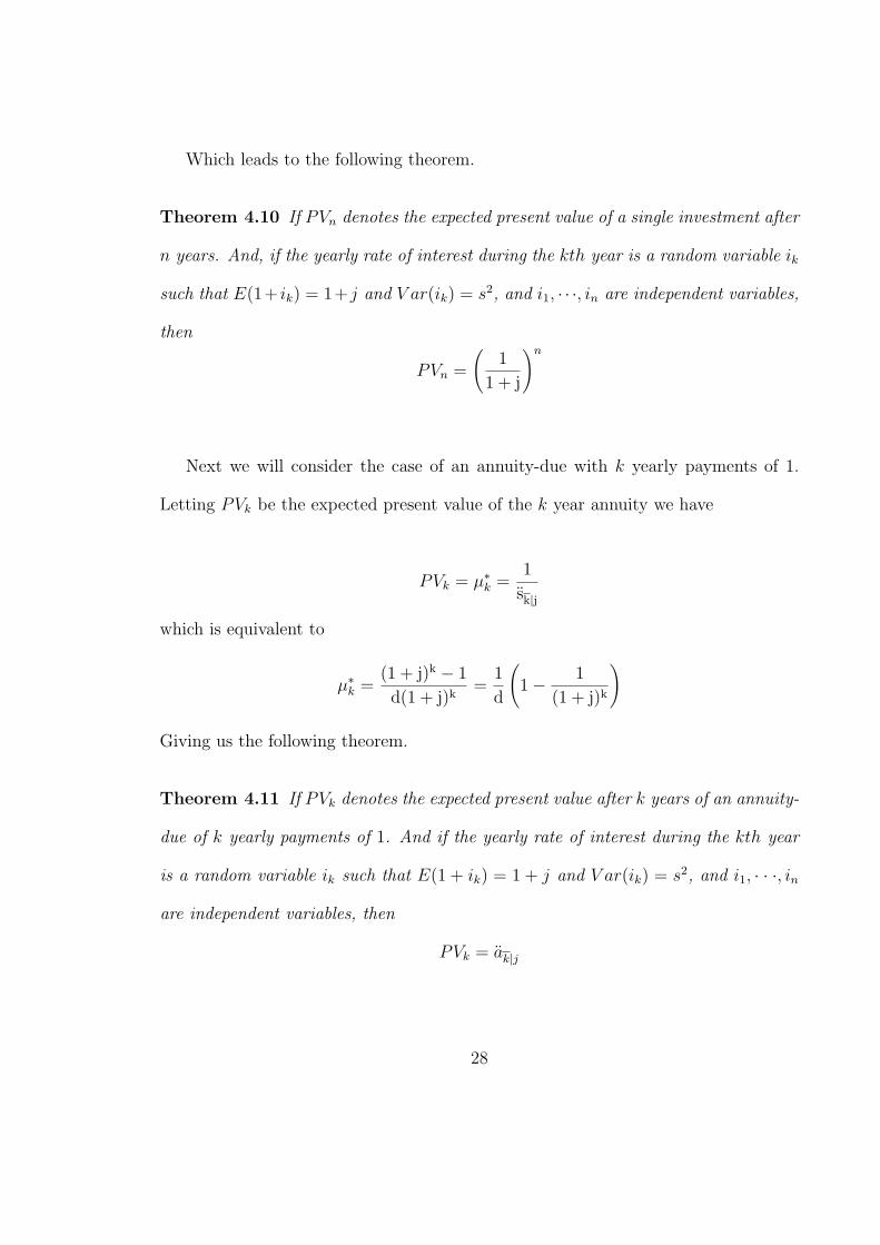
Which leads to the following theorem.

Theorem 4.10 If PVn denotes the expected present value of a single investment after

n years. And, if the yearly rate of interest during the kth year is a random variable ik

such that E(1+ ik) = 1+ j and V ar(ik) = s2, and i1, · · ·, in are independent variables,

then

PVn =

(1

1 + j

)n

Next we will consider the case of an annuity-due with k yearly payments of 1.

Letting PVk be the expected present value of the k year annuity we have

PVk = µ∗k =

1

sk|j

which is equivalent to

µ∗k =

(1 + j)k − 1

d(1 + j)k=

1

d

(1− 1

(1 + j)k

)

Giving us the following theorem.

Theorem 4.11 If PVk denotes the expected present value after k years of an annuity-

due of k yearly payments of 1. And if the yearly rate of interest during the kth year

is a random variable ik such that E(1 + ik) = 1 + j and V ar(ik) = s2, and i1, · · ·, in

are independent variables, then

PVk = ak|j

28

4.2 Life Annuities With Random Rates of Interest

The equations for life annuities in chapter 3 assume that time until death is a random

variable and the distribution is known. The interest rates in the models were assumed

to be constant. Yet examination of observed interest rates confirms this assumption

can be unrealistic. Thus in this section we will again consider the actuarial present

value of life annuities, but we will now assume both time until death and the rate of

interest are random variables.

We will assume there to be n possible values for our interest rate. We will denote

each of these as il where l ≤ n. As in previous work, we will assume that each

individual interest rate il has E(il) = j and V ar(il) = s2. And, 1E(1+il)

= 11+j

. Now

recall the actuarial present value of a life annuity with constant interest rates was

defined to be

ax = E[aK+1|] =∞∑

k=0

vkkpx.

Where K is the random variable defined as the number of complete future life years

of a life at age x. Now let ∗ax denote the actuarial present value of a life annuity with

random interest rates. Thus we must now consider the expectation with respect to

both K, and the interest rate il. We will assume that K and the i′ls are independent.

In addition we will introduce the actuarial notions EK to be the expectation with

respect to K, and Eil|K to be the expectation with respect to il given K. Thus we

can write

∗ax = EK Eil|K [il aK+1|].

29

Applying theorem 4.12 we obtain

∗ax = EK [aK+1|j].

Hence we have

∗ax =∞∑

k=0

ak+1|j kpx qx+k

or equivalently we can write

∗ax =∞∑

k=0

(1

1 + j

)k

kpx.

30

BIBLIOGRAPHY

31

[1] N.L. Bowers, Jr., H.U. Gerber, J.C. Hickman, D.A. Jones, and C.J. Nesbitt,

—em Actuarial Mathematics, The Society of Actuaries, Schaumburg, IL, 1997.

[2] W.L. Hart, Mathematics of Investment, D.C. Health and Company, (1958), 4.

[3] D. Hong, Course Packet for Actuarial Mathematics, East Tennessee State Uni-

versity, Spring 1999.

[4] S.G. Kellison, The Theory of Interest, Irwin, (1991), 2.

[5] S.G. Kellison, Fundamentals of Numerical Analysis, Irwin, (1975).

[6] A. Zaks, Annuities under random rates of interest. Insurance Mathematics &

Economics. 28 (2001) 1–11.

32

VITA

LESLEY J. BAKER

Education: East Tennessee State University, Johnson City, TN;Mathematics, B.S. 1999.

East Tennessee State University, Johnson City, Tennessee;Mathematics, M.S. 2001.

Professional MathLab Director,Experience: ETSU, August, 2000-August, 2001;

Graduate Assistant, East Tennessee State University;Johnson City, Tennessee, January 2001 – May 2001

Vice President of Actuarial Students Association,ETSU, Johnson City, Tennessee, August, 1999 – August, 2000.

President of Actuarial Students Association,ETSU, Johnson City, Tennessee, August, 2000 – August, 2001.

33