Life and Growth - Stanford Universityweb.stanford.edu/~chadj/LifeandGrowthJPE2016.pdf · Life and...

Life and Growth

Charles I. Jones

Stanford University and National Bureau of Economic Research

Tham gLicanat BeEconsity oNatioVijveras sup

Electro[ Journa© 2016

All us

Some technologies save lives—new vaccines, new surgical techniques,safer highways. Others threaten lives—pollution, nuclear accidents,global warming, and the rapid global transmission of disease. How isgrowth theory altered when technologies involve life and death insteadof just higher consumption? This paper shows that taking life into ac-count has first-order consequences. Under standard preferences, thevalue of life may rise faster than consumption, leading society to valuesafety over consumption growth. As a result, the optimal rate of con-sumption growth may be substantially lower than what is feasible, insome cases falling all the way to zero.

I. Introduction

Some technologies save lives—new vaccines, new surgical techniques, saferhighways. Others threaten lives—pollution, nuclear accidents, globalwarming, the rapid global transmission of disease, and bioengineered vi-ruses. How is growth theory altered when technologies involve life anddeath instead of just higher consumption?To begin, consider what might be called a “Russian roulette” theory of

economic growth. Suppose the overwhelming majority of new ideas are

is paper was previously circulated under the title “The Costs of Economic Growth.” Irateful to Raj Chetty, Christian Groth, Bob Hall, Peter Howitt, Pete Klenow, Omardro, David Romer, Michele Tertilt, Martin Weitzman, and participants in seminarsrkeley, Columbia, the Federal Reserve Bank of San Francisco, a National Bureau ofomic Research Economic Fluctuations and Growth meeting, Rand, Stanford, Univer-f California, Irvine, and University of California, San Diego, for comments and to thenal Science Foundation for financial support. Arthur Chiang, Jihee Kim, Williamberg, and Mu-Jeung Yang provided excellent research assistance. Data are providedplementary material online.

nically published March 8, 2016l of Political Economy, 2016, vol. 124, no. 2]by The University of Chicago. All rights reserved. 0022-3808/2016/12402-0002$10.00

539

This content downloaded from 171.067.216.021 on April 15, 2016 08:50:41 AMe subject to University of Chicago Press Terms and Conditions (http://www.journals.uchicago.edu/t-and-c).

540 journal of political economy

All

beneficial and lead to growth in consumption. However, there is a smallchance that a new idea will be dangerous and cause substantial loss oflife. Do discovery and economic growth continue forever in such a frame-work, or should society eventually decide that consumption is high enoughand stop playing the game of Russian roulette? How is this conclusion af-fected if researchers can also develop lifesaving technologies?This paper shows that taking life and death into account has first-order

consequences. The answers to these questions depend crucially on theshape of preferences. For a large class of conventional specifications, in-cluding log utility, the value of life rises faster than consumption, lead-ing society to value safety over consumption growth. As a result, the op-timal rate of consumption growth may be substantially lower than whatis feasible, in some cases falling all the way to zero.This project builds on a diverse collection of papers. Murphy and Topel

ð2003Þ, Nordhaus ð2003Þ, and Becker, Philipson, and Soares ð2005Þ em-phasize a range of economic consequences of the high value attachedto life. Murphy and Topel ð2006Þ extend this work to show that the eco-nomic value of future innovations that reduce mortality is enormous.Weisbrod ð1991Þ early on emphasized that the nature of health spend-ing surely influences the direction and rate of technical change. Hall andJones ð2007Þ—building on Grossman ð1972Þ and Ehrlich and Chumað1990Þ—is a direct precursor to the present paper, in ways that will be dis-cussed in detail below.1

The paper is organized as follows. Section II presents a simple versionof the “Russian roulette”model outlined above. Themodel is interestingin its own right, but it also serves to introduce the key role that the valueof life and the shape of preferences play in the analysis. A limitation ofthis framework is that it does not recognize that technological changearguably reduces mortality more than it increases it. Section III there-fore develops a richer model that features both “standard” ideas that raiseconsumption and “lifesaving” ideas that reduce mortality. This frame-work allows the growth rate to vary continuously, permitting a careful studyof the mechanisms highlighted in the simple model. Section IV discussesa range of empirical evidence that is helpful in judging the relevance ofthese results. Section V presents a calibration of the consumption growthslowdown and a numerical example illustrating that the asymptotic re-sults of the theory have similar implications for the transition path. Sec-tion VI presents conclusions.

1 Other related papers take these ideas in different directions. Acemoglu and Johnsonð2007Þ estimate the causal impact of changes in life expectancy on income. Malani andPhilipson ð2011Þ provide a careful analysis of the differences between medical researchand research in other sectors. Dalgaard and Strulik ð2014Þ model aging as the accumula-tion of “deficits” and consider how this process can be slowed by health spending.

This content downloaded from 171.067.216.021 on April 15, 2016 08:50:41 AM use subject to University of Chicago Press Terms and Conditions (http://www.journals.uchicago.edu/t-and-c).

life and growth 541

II. The Russian Roulette Model

A “Russian roulette” model of growth allows us to see some of the mainissues in this paper in the clearest way. Suppose the overwhelming major-ity of new ideas are beneficial and lead to consumption growth. However,there is a small chance that research will result in a disaster that kills somefraction of the population. What does growth look like in this setting?In the economy, a single agent is born at the start of each period and

lives for at most one period. The agent is endowed with some initial stockof knowledge that generates a consumption level c and has a utility func-tion uðcÞ5 �u 1 ½c12g=ð12 gÞ�. The parameter �u is a constant that will bediscussed in more detail below.The only decision faced by the agent is whether or not to conduct re-

search. With some ðhighÞ probability 12 p, research leads to a new ideathat increases consumption by the growth rate �g . With some small prob-ability p, however, the research results in a disaster that kills the agent.2

We are free to normalize the utility associated with death to any valueand therefore choose zero. Finally, if there is no research, consumptionremains constant at the level associated with the original stock of knowl-edge and there is no risk of a disaster.Expected utility for the two options “Research” and “Stop” is given by

U Research 5 ð12 pÞuðc1Þ1 p � 05 ð12 pÞuðc1Þ; c1 5 cð11 �g Þ;U Stop 5 uðcÞ:

The agent engages in research if U Research > U Stop. This condition is it-self amenable to analysis, but more intuition is available—intuition thatsheds light on the richer model I present later—if we take a first-orderTaylor expansion around uðcÞ. Using the approximation uðc1Þ ≈ uðcÞ1u0ðcÞ � ðc1 2 cÞ5 uðcÞ1 u0ðcÞ�g c, the agent chooses to undertake researchif

ð12 pÞu0ðcÞ�g c > puðcÞ:

This expression has a nice interpretation: the left side is the benefit ofengaging in research and the right side is the cost. For the benefit, withprobability 1 2 p the research is successful and increases consumptionby the amount �g � c, which gets converted into utility units by the conver-sion factor u0ðcÞ. On the cost side, with probability p, the research endsin failure and the utility flow uðcÞ never gets to be enjoyed.

2 Extending the model to include a population of representative agents, there is anequivalence in this setup between a fraction p of the existing population dying and the en-tire population facing a probability p of extinction. Both interpretations are useful.

This content downloaded from 171.067.216.021 on April 15, 2016 08:50:41 AMAll use subject to University of Chicago Press Terms and Conditions (http://www.journals.uchicago.edu/t-and-c).


All

Rearranging this expression, research occurs as long as

�g >p

12 p� uðcÞu0ðcÞc : ð1Þ

Because �g and p are both parameters, the key variable in this expressionis the term uðcÞ=u0ðcÞc. This term has a natural economic interpretation:uðcÞ is the value of life in utils, and dividing by u0ðcÞ converts this intoconsumption units. Therefore, this term is the value of life as a ratio tothe level of consumption.With uðcÞ5 �u 1 ½c12g=ð12 gÞ�, this value of life expression is

uðcÞu0ðcÞc 5 �ucg21 1

1

12 g: ð2Þ

It turns out to be convenient to analyze three cases separately: g < 1, g > 1,and log utility ðg 5 1Þ.

A. Exponential Growth: 0 < g < 1

To begin, let us assume g < 1 and set �u 5 0, as this parameter does notplay a crucial role in this case.With these parameter restrictions, the valueof life relative to consumption in ð2Þ is constant and equal to 1=ð12 gÞ.Substituting back into ð1Þ, research continues forever as long as �g is suf-ficiently large relative to the probability of a research disaster. In this case,the economy will grow exponentially across generations, apart from raredisasters. Of course, each generation is also taking a risk, and occasionallya research disaster kills off a generation before they can enjoy the utilityassociated with consumption.3

B. The End of Growth: g > 1

With g > 1, the constant �u plays an essential role. In particular, recall thatI have normalized the utility associated with “death” to be zero: the indi-vidual gets uðcÞ if she lives and gets zero if she dies. But this means thatuðcÞ must be greater than zero for life to be worth living. Otherwise,death is preferred to life.Withg>1, however, c12g=ð12 gÞ is less than zero.For example, this flow is21/c forg5 2.Anobviousway tomakeour prob-lem interesting is to add a positive constant to flow utility, and this moti-vates the introduction of �u, which represents the upper bound for utility.4

3 Without using the Taylor series approximation, the exact condition for research tocontinue is ð12 pÞð11 �g Þ12g > 1. If one allows for �u > 0, then the value of life relative toconsumption is initially even higher but then falls asymptotically to 1=ð12 gÞ, so the sameconditions apply.

4 There exists a value of consumption below which flow utility is still negative. Below thislevel, individuals would prefer death to life; see Rosen ð1988Þ. This level is very low for plau-


life and growth 543

Assuming g > 1 and �u > 0, notice that the value of life relative to con-sumption in equation ð2Þ increases with consumption. That is, as eachgeneration gets richer, life becomes increasingly valuable relative to con-sumption. Substituting this expression back into the research choice inequation ð1Þ then leads to the following result: When consumption issmall, each generation chooses to engage in research. However, even-tually society becomes sufficiently rich that the gains from higher con-sumption growth are outweighed by the risks of a disaster and economicgrowth comes to an end.Without making the Taylor series approximation, this choice can be

illustrated graphically, as in figure 1, and the same basic conclusion fol-lows: once society reaches ðor exceedsÞ consumption level c *, no addi-tional research is undertaken and growth stops.

C. Log Utility

The case of log utility is more subtle. In contrast to the case of g > 1, flowutility is unbounded in the log case. However, it turns out that growth

FIG. 1.—The research decision when g > 1. As long as consumption is less than c*, eachgeneration engages in research. Once consumption reaches ðor exceedsÞ c*, even a tinyrisk of a research disaster is not worth taking because life becomes too valuable. Color ver-sion available as an online enhancement.

sible parameter values and can be ignored here. The role of the constant in flow utility isalso discussed by Murphy and Topel ð2003Þ, Nordhaus ð2003Þ, Becker et al. ð2005Þ, andHall and Jones ð2007Þ.



All

eventually ceases in this case as well. The value of life expression inthe log case is uðcÞ=u0ðcÞc 5 �u 1 logc. So even in this case the value of liferises relative to consumption and the condition in ð1Þ for research tocontinue is eventually violated.5

D. Summary of the Russian Roulette Model

The simple model illustrates that a key consideration in the trade-off be-tween safety and consumption growth is the value of life relative to con-sumption. If the value of life rises more slowly than consumption ðg < 1Þ,then safety considerations fade in importance and growth continues for-ever. However, if the value of life rises faster than consumption, safetyconsiderations become increasingly important over time and can even-tually lead to a cessation of research and consumption growth.

III. Life and Growth in a Richer Setting

The Russian roulette model in the previous section is elegant and deliv-ers intuitive results for the interaction between safety and growth. How-ever, that setup ignores the important possibility that research can makethe world safer rather than more dangerous. Medical innovations, anti-lock brakes, and autopilots for airplanes are examples of technologiesthat save lives rather than endanger them. The simple model also treatsgrowth as a “black box.”In this section, I address these concerns by adding safety consider-

ations to a standard growth model based on the discovery of new ideas.The result deepens our understanding of the interactions between safetyand growth. For instance, in this framework, concerns for safety can slowthe rate of consumption growth ðe.g., from 4 percent to 1 percentÞ butwill never lead to a steady-state level of consumption. The model alsohighlights the distinction between GDP growth and consumptiongrowth: here, it is only the latter that is affected.The model below can be viewed as combining the “direction of tech-

nical change” work by Acemoglu ð2002Þ with the health spending modelof Hall and Jones ð2007Þ. That is, I posit a standard idea-based growthmodel in which there are two types of ideas instead of one: ideas that en-hance consumption and ideas that save lives. The key allocative decisionsin the economy are ðiÞ how many scientists to put into the consumptionversus lifesaving sectors and ðiiÞ how many workers to put into using theseideas to manufacture goods.

5 Without taking the Taylor approximation, we get the same result: the condition for re-search to continue is ð12 pÞlogð11 �g Þ > pð�u 1 logcÞ.


life and growth 545

A. The Economic Environment

The economy features two main sectors, a consumption sector and a life-saving sector. On the production side, both sectors are quite similar, andeach looks very much like the Jones ð1995Þ version of the Romer ð1990Þgrowth model. In fact, I will purposefully make the production side ofthe two sectors as similar as possible ði.e., using the same parametersÞso it will be clear where the results come from.Total production of the consumption good Ct and the lifesaving good

Ht are given by

Ct 5 EAt

0

x1=ð11aÞit di

" #11a

and Ht 5 EBt

0

z1=ð11aÞit di

" #11a

: ð3Þ

Each sector uses a variety of intermediate goods to produce output withthe same basic production function. The main difference is that differ-ent varieties—different ideas—are used for each sector: At represents therange of technologies available to produce consumption goods, while Bt

represents the range used to produce lifesaving goods. It might be help-ful to think of the zit as purchases of different types of pharmaceuticalsand surgical techniques. But I have in mind a broader category of goodsas well, such as pollution scrubbers in coal plants, seatbelts and airbags,child safety locks, lifeguards at swimming pools, and warning labels oncigarettes.Once the blueprint for a variety has been discovered, one unit of labor

can be used to produce one unit of that variety. The number of peopleworking as labor is denoted Lt, so the resource constraint for this labor is

EAt

0

xitdi

︸�Lct

1EBt

0

zitdi

︸�Lht

� Lt : ð4Þ

People can produce either goods, as above, or ideas. When they pro-duce ideas, we call them scientists, and the production functions for newideas are given by

_At 5 Sl

atAf

t and _Bt 5 Sl

btBf

t ; ð5Þwhere I assume f < 1. Once again, notice that I assume the same param-eters for the idea production functions in the two sectors; this assump-tion could be relaxed but is useful because it helps to clarify where themain results come from.The resource constraints on scientists and people more generally are

Sat 1 Sbt � St ð6Þ



All

and

St 1 Lt � N t : ð7Þ

That is, Nt denotes the total number of people, who can work as scien-tists or labor. In turn, scientists and labor can work in either the consump-tion sector or the lifesaving sector.Next, consider mortality. Individuals face a time-varying mortality rate dt.

The probability that an agent born at date 0 survives to date t is given by

Mt 5 e2∫t

0dsds:

Equivalently, the law of motion for this survival probability is

_Mt 52dtMt ; M 0 5 1: ð8ÞThe mortality rate is endogenous and can be reduced by purchasing life-saving goods. An individual who purchases ht � Ht=Nt faces a mortalityrate

dt 5 h2b

t : ð9ÞExpected lifetime utility, taking mortality into account, is then

U 5E∞

0

e2rtuðctÞMtdt: ð10Þ

See Arthur ð1981Þ, Rosen ð1988Þ, and Murphy and Topel ð2006Þ for sim-ilar formulations of expected utility with time-varying mortality.As discussed earlier, I specify flow utility as

uðctÞ5 �u 1c12gt

12 g; ct � Ct=N t : ð11Þ

Flow utility takes a standard form, augmented by a constant �u, whichis related to the overall value of life versus death.6

Finally, for population growth, there are two relatively natural ways toproceed. One can assume exogenous fertility so that reductions in mor-tality raise population growth. Alternatively, one can assume that fertil-ity adjusts so that the rate of population growth is exogenously constant.It turns out that the main results go through in either case. I assume thelatter here, so that population growth occurs at a constant positive rate:7

_Nt 5 �nNt : ð12Þ

6 As usual, r must be sufficiently large given growth so that utility is finite.7 The working paper version in Jones ð2011Þ considers the former case.


life and growth 547

B. Allocating Resources

This economic environment features 14 unknowns—Ct, Ht, ct, ht, At, Bt, xit,zit, Sat, Sbt, St, Lt,Mt, dt—and 11 equations—equations ð3Þ–ð9Þ, together withthe definitions for ht and ct ðI am not counting lifetime utility, flow utility,and the exogenous population process in this numerationÞ.There are, not surprisingly then, three key allocative decisions that have

to be made in the economy, summarized by three allocative fractions st,ℓt, and jt :

1. How many scientists make consumption ideas versus lifesavingideas: st � Sat=St .

2. How many workers make consumption goods versus lifesavinggoods: ‘t � Lct=Lt . ðGiven the symmetry of the setup, it is efficientto allocate the xit and the zit symmetrically across varieties, so I willjust impose this throughout the paper to simplify things.Þ

3. How many people are scientists versus workers: jt � St=Nt .

C. A Rule of Thumb Allocation

For reasons that will become clear, it is convenient to begin with a simple“rule of thumb” allocation, analogous to Solow’s assumption of a fixedsaving rate in his version of the neoclassical growth model.In particular, consider the following rule of thumb allocation: st 5 �s, ‘t 5 �‘,

and jt 5 �j, where each of these new parameters is between zero andone. That is, consider putting a fixed fraction of the scientists in each re-search sector and a fixed fraction of the workers in each goods sector,and let a fixed fraction of the population work as scientists.It is straightforward to show the following result.Proposition 1 ðBGP under the rule of thumb allocationÞ. Under the

rule of thumb allocation, where st 5 �s, ‘t 5 �‘, and jt 5 �j, all between zeroand one, there exists a balanced growth path ðBGPÞ such that

g *A5 g *

B5

l�n

12 f; ð13Þ

g *c5 g *

h5 ag *

A5 ag *

B5 �g � al�n

12 f; ð14Þ

and

g *d 52b�g ; dt ! 0: ð15Þ

This is basically the expected outcome in a growth model of this fla-vor. With labor allocated symmetrically within the consumption and lifesectors, the production functions are Ct 5 Aa

t Lct and Ht 5 Bat Lht . No-



All

tice that each production function exhibits increasing returns to scalemeasured by a, reflecting the nonrivalry of both kinds of ideas. Theidea production functions are also symmetric in form. For instance,_At=At 5 Sl

at=A12f

t . So along a BGP, Sl

at and A12f

t must grow at the samerate. Since the growth rate of scientists is pinned down by the popula-tion growth rate, this means that the growth rate of At ðand BtÞ will be aswell. Therefore, Bt goes to infinity, which means that the mortality ratedt falls to zero, and so on.The rule of thumb allocation suggests that this model will deliver a

BGP with ever-increasing life expectancy. Moreover, growth is balancedin a particular way: technical change occurs at the same rate in both theconsumption and life sectors, so the relative price of the consumptionand life aggregates is constant. And by assumption, a constant fractionof labor and scientists work in each sector. Of course, I could have alteredsome of these results simply by making the elasticity of substitution orthe parameters of the idea production function differ between the twosectors. But that is not where I wish to go. For the moment, simply notethat everything is nicely behaved and straightforward in the rule of thumballocation.

D. The Optimal Allocation

Somewhat surprisingly, the rule of thumb allocation turns out not to bea particularly good guide to the dynamics of the economy under the op-timal allocation. Instead, as suggested by the Russian roulette model atthe start of this paper, there is a sense in which consumption growth isslower thanwhat is feasible because of a shift in the allocation of resourceswhen diminishing returns to consumption are sufficiently strong.There are many interesting questions related to welfare theorems

in this type of model: is a decentralized market allocation efficient? Onecan imagine various externalities related to safety, particularly when “ex-istential” risks are under consideration. For now, however, I put these in-teresting questions aside. My concern instead is with how safety consid-erations affect the economy even when resources are allocated optimally.The optimal allocation of resources is a time path for ct, ht, st, ℓt, jt, At,

Bt, Mt, dt that maximizes the utility of a representative agent, solving thefollowing problem:

maxfst ;‘t ;jtg

U 5E∞

0

MtuðctÞe2rtdt ð16Þ

subject to

ct 5 Aa

t ‘tð12 jtÞ; ð17Þ


life and growth 549

ht 5 Ba

t ð12 ‘tÞð12 jtÞ; ð18Þ

_At 5 slt jl

t Nl

t Af

t ; ð19Þ

_Bt 5 ð12 stÞljl

t Nl

t Bf

t ; ð20Þ

_M t 52dtM t ; dt 5 h2b

t : ð21Þ

Note that other definitions of “optimal” are possible here; for example,the representative agent here does not care about future generations.The results below would continue to hold even with altruistic individualsor with a social welfare function that puts weight on future generations.The “selfish” approach here illustrates that none of the results come fromthese additional considerations.8

To solve for the optimal allocation, I define the Hamiltonian:

H5MtuðctÞ1 patslt j

l

t Nl

t Af

t 1 pbtð12 stÞljl

t Nl

t Bf

t 2 vtdtM t ; ð22Þ

where ct 5 Aa

t ‘tð12 jtÞ and dt 5 h2b

t 5 ½Bat ð12 ‘tÞð12 jtÞ�2b. The costate

variables—pat, pbt, and vt—capture the shadow values of an extra con-sumption idea, an extra lifesaving idea, and an extra lifetime ðresettingM to oneÞ to maximized welfare.Using the maximum principle and solving the first-order necessary

conditions for the optimal allocation, we can derive several results. Themost important of these is given in the next proposition ðproofs are rel-egated to App. AÞ.9Proposition 2 ðOptimal growth with g > 11 bÞ. Assume that the mar-

ginal utility of consumption falls rapidly, in the sense that g > 11 b. Thenthe optimal allocation features an asymptotic constant growth path suchthat as t → ∞, the fraction of labor working in the consumption sector ℓt

8 For example, one could multiply flow utility by the size of the population Nt in eq. ð16Þto include weight on future generations, but this is essentially equivalent to changing therate of time preference.

9 The argument that these first- order conditions characterize the solution is more sub-tle than usual. The standard very stringent Arrow/Mangasarian conditions for concavity donot hold for this problem, nor even for Jones ð1995Þ ðdespite the fact that they hold forRomer [1990]!Þ. However, Romer ð1986Þ developed a different approach for growth mod-els with increasing returns, and that approach works here: one can use the arguments inRomer ð1986Þ to show that there exists a solution to this problem and show that it is inte-rior. Since the first-order conditions characterize any interior solution and they identify aunique path here, it must indeed be the solution.



All

and the fraction of scientists making consumption ideas st both fall tozero at constant exponential rates, and asymptotic growth is given by10

g *s5 g *

‘ 52�g ðg2 12 bÞ

11 ðg2 1Þ 11al

12 f

� � < 0; �g � al�n

12 f; ð23Þ

g *A5

lð�n 1 g *sÞ

12 f; g *

B5

l�n

12 f> g *

A; ð24Þ

g *d 52b�g ; g *

h5 �g ; ð25Þ

g *c5 ag *

A1 g *

‘ 5 �g �11 b 11

al

12 f

� �

11 ðg2 1Þ 11al

12 f

� � < �g : ð26Þ

This proposition echoes the key result from the Russian roulette modelat the start of the paper: if the marginal utility of consumption runs intosufficiently sharp diminishing returns, safety considerations alter the es-sential nature of optimal growth. While in the earlier setup it was possiblefor consumption growth to cease, the model given here displays a moresubtle result.First, the economy optimally settles down to an asymptotic constant

growth path ðone in which all variables grow at constant ratesÞ. However,along this path, consumption grows at a rate that is slower than what isfeasible. This can be seen by comparing the consumption growth ratesfor the rule of thumb allocation in ð14Þ and the optimal allocation inð26Þ: when g 2 1 > b, g *

c< �g .

Second, the proximate cause of this slower growth is an exponentialshift in the allocation of resources. Both the fraction of scientists andthe fraction of workers engaged in the consumption sector—st and ℓt—fallexponentially over time along the BGP.To see how this shift slows growth, recall the production functions for

ideas, writing them as follows:

_Bt

Bt

5ð12 stÞljl

t Nlt

B12ft

and _At

At

5slt j

lt N

lt

A12f

t

:

The share 1 2 st in the lifesaving sector converges to one, leading tothe expected result for gB: since jt is also constant asymptotically, a con-

10 These results, and indeed the results throughout the remainder of this paper, havethe following form: limt!∞g ct

5 g *c, and so on.


life and growth 551

stant value of _Bt=Bt requires Nlt and B12f

t to grow at the same rate; there-fore, g *

B 5 l�n=ð12 fÞ. In contrast, the share st in the consumption ideasproduction function falls exponentially toward zero. The exponentialshift of scientists out of this sector means that a constant _At=At occursif and only if slt N

lt and A12f

t grow at the same rates. But in this case, theshift of scientists out of the consumption sector leads the numerator togrow more slowly than l�n, leading to g *

A 5 lðg *s1 �nÞ=ð12 fÞ. The nega-

tive trend in st slows growth in At relative to what is feasible with a con-stant allocation of scientists.This result makes a clear prediction: we should see the composition

of research shifting over time away from consumption ideas and towardlifesaving ideas if the model is correct and if the marginal utility of con-sumption falls sufficiently fast. I will provide empirical evidence on thisprediction later in the paper.To understand the fundamental cause for this structural change in the

economy, consider the following equation, which is the first-order con-dition for allocating labor between the consumption and life sectors:

12 ‘t‘t

5 bdtvt

u0ðctÞct : ð27Þ

The left side of this equation is just the ratio of labor working in thelife sector to labor working in the consumption sector. This equation saysthat the ratio of workers is proportional to the ratio of what these work-ers can produce. In the numerator is the death rate dt multiplied by thevalue of a life in utils, vt: this is the total value of what can potentiallybe gained by making a lifesaving good. The denominator, in contrast,is proportional to what can be gained by making consumption goods:the level of consumption multiplied by the marginal utility of consump-tion to put it in utils, as in the numerator.In the analysis of this equation, it turns out to be useful to define ~v t �

vt=u0ðctÞct : the value of a life in consumption units as a ratio to the level

of consumption. This is the analogue to uðcÞ=u0ðcÞc in the Russian rou-lette model, where lives last for one period; in fact, one can show—seeequation ðA4Þ in Appendix A—that the two are proportional here.The allocation of workers then depends on the product dt~vt . In fact,

as shown in Appendix A, the allocation of scientists depends on exactlythis same term; see equation ðA3Þ. Over time, the number of deaths thatcan potentially be avoided, dt, declines. However, the value of each liferises. When g > 1, the value of life rises even as a ratio to consumption,so ~vt rises. Then it is a race: dt falls at a rate proportional to b, while ~vt

rises at a rate proportional to g 2 1; hence the critical role of g 2 1 2 b.In particular, when g is large, as in the proposition just stated, the valueof life rises very rapidly, so that dt~vt rises to infinity. In this case, the op-timal allocation shifts all the labor and scientists into the life sector: the



All

value of the lives that can be saved rises so fast that it is optimal to devoteever-increasing resources to saving lives.

E. The Optimal Allocation with g < 1 1 β

What happens if the marginal utility of consumption does not fall quiteso rapidly? The intuition is already suggested by the analysis just provided,and the result is given explicitly in the next proposition.Proposition 3 ðOptimal growth with g < 1 1 bÞ. Assume that the

marginal utility of consumption falls, but not too rapidly, in the sensethat g < 1 1 b. Then the optimal allocation features an asymptotic con-stant growth path such that as t → ∞, the fraction of labor working inthe life sector ~‘t � 12 ‘t and the fraction of scientists making lifesavingideas ~st � 12 st both fall to zero at constant exponential rates, and as-ymptotic growth is given by

g *A5

l�n

12 f; g *

B5

lð�n 1 g *~s Þ

12 f< g *

A;

g *c5 �g � al�n

12 f; g *

d 52bg *h;

and the exact values for g~s* and g *h depend on whether g > 1 or g ≤ 1.

In particular, if 1 < g < 11 b,

g *~s 5 g *

~‘5

2�g ðb1 12 gÞ11 b 11

al

12 f

� � < 0; ð28Þ

g *h5 �g �

11 ðg2 1Þ 11al

12 f

� �

11 b 11al

12 f

� �2664

3775 < �g : ð29Þ

While if g ≤ 1,

g *~s 5 g *

~‘5

2b�g

11 b 11al

12 f

� � < 0; ð30Þ

g *h5 �g � 1

11 b 11al

12 f

� �2664

3775 < �g : ð31Þ


life and growth 553

This proposition shows that when g < 1 1 b, the results flip-flop. Thatis, there is still a trend in the allocation of scientists and workers, butthe trend is now away from the health/life sector and toward the con-sumption sector. In this case, the death rate falls faster than the value oflife rises. Looking back at equation ð27Þ, the denominator u0ðctÞct risesfaster than the numerator: the greater gain is in providing consump-tion goods rather than in saving lives. We once again get an unbalancedgrowth result, but now it is the consumption sector that grows faster.

F. “Interior” Growth When g 5 1 1 β

Proposition 4 ðOptimal growth with g 5 1 1 bÞ. Assume the fol-lowing knife-edge condition relating preferences and technology: g 51 1 b. Then the optimal allocation features an asymptotic balancedgrowth path such that as t → ∞, the key allocation variables ℓt and st settledown to constants strictly between zero and one, and asymptotic growthis given by

g *A5 g *

B5

l�n

12 f;

g *c5 g *

h5

al�n

12 f5 �g ; g *

d 52b�g :

This is the one case in which growth is “balanced” in the sense that theconsumption and life sectors grow at the same rate and labor and scien-tists do not all end up in one sector. But, as stated above, this requires asomewhat arbitrary knife-edge condition relating technology and prefer-ences. The intuition for this knife edge is that the model features twogoods: consumption, whose marginal utility falls at rate 1 2 g, and h,whose marginal utility falls at rate b. Unless these two rates are the same,the allocation will tilt in one direction or the other.

G. Discussion

Several points now merit discussion. First, the results suggest that growthin one sector is slower than what is feasible. What about overall GDPgrowth? To answer this question, one needs to construct a measure ofGDP for this two-sector economy. Per capita GDP is p

cc 1 p

hh. We choose

consumption as our numeraire ðpc ; 1Þ. The relative price of h is theneasy to obtain in this economy: given that one unit of labor can produceeither Aa units of consumption or Ba units of the lifesaving good, the rel-ative price of h is the marginal rate of transformation ðA/BÞa.The growth rate of per capita GDP can then be calculated using the

Divisia method, as a weighted average of the growth rates of c and h,



All

where the weights are the nominal shares of c and h in GDP. Perhaps notsurprisingly, it turns out that the share of consumption in GDP, p

cc=ðp

cc 1

phhÞ, is equal to ℓ, the share of labor working in the consumption sector.

Per capita GDP growth is then ‘gc1 ð12 ‘Þg

h. But this means that GDP

growth is asymptotically equal to �g in all three cases above.11 Our key re-sult is about the composition of growth, and especially about the growthrate of consumption relative to what is feasible, rather than being a state-ment about overall GDP growth.Next, notice another important point: the Russian roulette model at

the start of the paper and the richer model developed subsequently leadto slightly different conclusions. In the Russian roulette model, consump-tion growth falls to zero when the marginal utility of consumption dimin-ishes rapidly, while in the richer model consumption growth is only slowedby some proportion. Why the difference?The answer turns on functional forms and modeling choices about

which we have relatively little information. In the Russian roulette model,the mortality rate depends on the growth rate of the economy rather thanon the level of technology, and this difference is evidently important. Pre-serving life there requires the growth rate to fall all the way to zero. Onecould enrich the Russian roulette model, for example, by embedding itin a Schumpeterian quality ladder model as in Aghion and Howitt ð1992Þ,where each idea increases consumption by a constant percentage whilehaving a small risk of a disaster. One could even add a second lifesavingtechnology to this framework. Nevertheless, since the mortality rate andthe growth rate of consumption would be linked, the logic just providedsuggests that consumption growth would still optimally fall to zero in thecase in which marginal utility declines rapidly.In this sense, the Russian roulette model and the richer model of Sec-

tion III are complements rather than substitutes. The general result is thatconcerns for safety can slow consumption growth, with the precise natureof the slowdown depending on modeling details.

IV. Empirical Evidence

The main model in this paper makes stark predictions regarding thecomposition of research. Depending on the relative magnitudes of g 2 1and b, the direction of technical change should shift either toward oraway from lifesaving technologies. In particular, if g is large—so that themarginal utility of consumption declines rapidly—one would expect tosee the composition of research shifting toward lifesaving technologies,thereby slowing consumption growth.

11 Intuitively, workers and researchers are leaving the slow-growing sector; indeed, it isthis fact that makes it slow growing. The sector they are attracted to does not suffer thisdepletion and grows at the expected semi-endogenous rate.


life and growth 555

In this section, I discuss a range of evidence on b, g, and the compo-sition of research. While not entirely decisive, the bulk of the evidenceis consistent with the first case considered, where there is an income ef-fect for livesaving technologies and consumption growth is slowed.Some general caveats should be noted before turning to the evidence.

The analysis so far has considered an allocation chosen by a social plan-ner. The evidence below, however, comes from real-world economies thatfeaturea rangeof institutions, taxes, and imperfections.Onecanshow thatsimple equilibrium allocations in our model ðe.g., a Romer-style equilib-rium with imperfect competitionÞ would also display trends in allocationsin the same cases, but this distinction is still worth noting. Second, the “life-saving” sector in the model and the “health” sector in the data are not thesame thing. The former includes goods such as fences around swimmingpools and safer highways, while the latter includes cosmetic surgery andknee replacements. The overall point of the evidence below is not to testthe model but rather to suggest that the case in which consumption growthis slowedmay be empirically relevant.

A. The Composition of Research

One might think that the main prediction on the composition of re-search would be an easy prediction to test: surely there must be readilyavailable statistics on research spending by the health sector of the econ-omy. Unfortunately, this is not the case. The main reason appears to bethat both the spending and performance of health research are donein several different organizations in the economy: industry, government,nonprofits, and academia. Thus, the construction of such numbers re-quiresmerging the results of different surveys, being careful to avoid dou-ble counting, considering changes in the surveys over time, and so on. Be-tween the 1970s and the early 1990s, the National Institutes of HealthðNIHÞundertook this calculation and reported a health researchnumber.But, unfortunately, I have not been able to find any other source that doesthis for the last 20 years.Figure 2 shows the original NIH numbers for the United States, along

with several attempts to extend this series to more recent years. Detailsare discussed in Appendix B.12 In addition to the original NIH estimates,figure 2 shows three other series. The longest is noncommercial healthresearch from the National Health Expenditure Accounts of the Cen-ters for Medicare and Medicaid Services ðCMMSÞ. The remaining twoseries add estimates of commercial research to the CMMS estimate, us-ing two different collections of surveys by the National Science Founda-tion ðNSFÞ. The fact that the NIH series and the CMMS1NSF series co-incide during overlapping years is somewhat reassuring.

12 I am grateful to Raymond Wolfe for guidance and suggestions with these data.



All

Figure 2 indicates that whether we look at noncommercial researchor the broader estimates for total research, the composition of R&D ap-pears to be shifting distinctly toward health over time. For example, theearliest estimates from 1960 suggest that the health sector accounted foronly about 7 percent of all R&D, while the most recent estimates from2007 are around 25 percent.Lifesaving technologies are invented around the world, not just in the

United States. Figure 3 uses OECD sources to study how the compositionof R&D is changing internationally. These data are available only since1991 but tell the same basic story: the composition of research is shiftingdistinctly toward health. In 1991, around 9 percent of OECD researchspending was on health, and this share rose to 16 percent by 2006. Thefigure also shows the corresponding share for the United States ðestimatedusing slightly different assumptions with theseOECD sourcesÞ, confirmingthe sharp rise that we saw earlier in figure 2.Of course, there are other possible explanations for the changing

composition of research. Perhaps the rise in the share of health spend-ing in the economy is due to other factors ðe.g., the insurance systemfavoring expensive technologies as in Weisbrod [1991]Þ, and health re-search is simply responding to these factors as well.

FIG. 2.—The changing composition of US R&D spending. The graph shows the risein the share of R&D spending in the United States that is devoted to health, accordingto several different measures. See Appendix B for sources and methodology. Color versionavailable as an online enhancement.


life and growth 557

B. Patents

As an alternative to looking at the inputs to idea production, one canconsider the output. Figure 4 shows the fraction of all patents grantedby the US Patent Office between 1963 and 1999 for medical equipmentand pharmaceuticals.13 There are well-known limitations to using the pat-ent data as a measure of idea production ðe.g., the distribution of patentvalues is very skewed; see Griliches [1990] for a detailed discussionÞ. How-ever, as one of many pieces of evidence, patents are useful. The share ofpatents for medical equipment and pharmaceuticals rises from around4 percent in 1963 to more than 13 percent in 1999. The dashed linein the figure shows one alternative cut of the data, restricting the uni-verse to patents by US innovators. Similar strong upward trends can befound in other cuts of the data: just restricting to foreign innovators orfor medical equipment and patents separately.

C. Empirical Evidence on β

The parameter b is readily interpreted as the elasticity of the mortalityrate with respect to real lifesaving expenditures. A rough estimate for

FIG. 3.—The changing composition of OECD R&D spending. The trend toward healthis apparent in OECDmeasures of R&D expenditures as well. The OECD estimate reportedhere includes data from the United States, Canada, France, Germany, Italy, Japan, Spain,and the United Kingdom. See Appendix B for sources and methodology. Color versionavailable as an online enhancement.

13 These data have been provided by Jeffrey Clemens and are discussed in detail in Clem-ens ð2013Þ.



All

this parameter can be obtained by considering the relative trends inmor-tality and health spending: this calculation attributes all the decline inmortality to health spending, which is probably an overestimate giventhe contributionof other factors such as education to decliningmortality.According to Health, United States 2009, age-adjusted mortality rates

fell at an average annual rate of 1.2 percent between 1960 and 2007, whileconsumer price index ðCPIÞ deflated health spending rose at an averageannual rate of 4.1 percent.14 The ratio of these two growth rates gives anestimate for b of 0.291. Hall and Jones ð2007Þ conduct a more formal anal-ysis along these lines using age-specific mortality rates and age-specifichealth spending and allowing for other factors to enter. For people be-tween the ages of 20 and 80, they find estimates for this elasticity rangingfrom 0.10 to 0.25. These different estimates suggest that values of b sub-stantially below one are plausible.

D. Estimates of γ

Given the estimates for b just reported, life considerations may domi-nate in the model if g is larger than about 1.3. In the most common

FIG. 4.—The fraction of patents for medical equipment or pharmaceuticals. “Total” re-fers to all patent grants in the NBER Patent Database. “US only” restricts the sample to pat-ents granted to US innovators. See Clemens ð2013Þ. Color version available as an onlineenhancement.

14 See tables 26 and 122 of that publication, available at http://www.cdc.gov/nchs/hus.htm.


life and growth 559

way of specifying preferences for macro applications, the coefficient ofrelative risk aversion, g in our notation, equals the inverse of the elas-ticity of intertemporal substitution. Large literatures on asset pricingðLucas 1994Þ and labor supply ðChetty 2006Þ suggest that g > 1 is a reason-able value, and values above 1.5 are quite common in this literature.Evidence on the elasticity of intertemporal substitution, 1/g in our

notation, is more mixed. The traditional view, such as Hall ð1988Þ, is thatthis elasticity is well below one, consistent with the case of g > 1.3. Thisview is supported by a range of careful microeconometric work, includ-ing Attanasio andWeber ð1995Þ, Barsky et al. ð1997Þ, and Guvenen ð2006Þ;see Hall ð2009Þ for a survey of this evidence. On the other hand, Vissing-Jorgensen and Attanasio ð2003Þ and Gruber ð2006Þ find evidence thatthe elasticity of intertemporal substitution is greater than one, suggestingthat g < 1 could be appropriate.Empirical evidence on the value of life.—Direct evidence on how the value

of life changes with income—another way to gauge the magnitude ofg—is surprisingly difficult to come by. Most of the empirical work in thisliterature is cross-sectional in nature and focuses on getting a single mea-sure of the value of life ðor perhaps a value by ageÞ; see Ashenfelter andGreenstone ð2004Þ, for example. There are a few studies that containimportant information on the income elasticity, however. Viscusi andAldy ð2003Þ conduct a meta-analysis and find that across studies, the valueof life exhibits an income elasticity below one. On the other hand, Ham-mitt, Liu, and Liu ð2000Þ and Costa and Kahn ð2004Þ consider explicitlyhow the value of life changes over time. These studies find that the valueof life rises roughly twice as fast as income, consistent with a value of garound 2.Evidence from health spending.—The key mechanism at work in this

paper is that the marginal utility of consumption falls quickly if g > 1,leading the value of life to rise faster than consumption. This tilts the al-location in the economy away from consumption growth and toward pre-serving lives. Exactly this same mechanism is at work in Hall and Jonesð2007Þ, which studies health spending. In that paper, g > 1 leads to an in-come effect: as the economy gets richer over time ðexogenouslyÞ, it is op-timal to spend an increasing fraction of income on health care in an effortto reduce mortality. The same force is at work here in a very different con-text. Economic growth combines with sharply diminishing marginal util-ity to make the preservation of life a luxury good. The novel finding is thatthis force has first-order effects on the determination of economic growthitself.Figure 5 shows international evidence on health spending as a share

of GDP. This share is rising in many countries of the world, not onlyin the United States. Indeed, for the 16 OECD countries reporting data



All

in both 1971 and 2010 ðmany not shownÞ, all experienced a rising healthshare.15

E. Growth in Health and Nonhealth Consumption

The results from our model suggest that, apart from a knife-edge case,the composition of research will shift toward either the consumptionsector or the lifesaving sector. Moreover, at least insofar as the parame-ters of the idea production function are similar in those two sectors ðandwe have no real evidence pushing us one way or the other on thisÞ, thesector that sheds its researchers will grow more slowly in the long run.This prediction prompts us to look at the historical evidence on the

growth of per capita consumption for both the health and nonhealth

FIG. 5.—International evidence on the income effect in health spending. Data are fromOECDHealth Data 2012 and are reported every 10 years. Color version available as an onlineenhancement.

15 Acemoglu, Finkelstein, and Notowidigdo ð2009Þ estimate an elasticity of hospitalspending with respect to transitory income of 0.7, less than one, using oil price movementsto instrument local income changes at the county level in the southern part of the UnitedStates. ðThe instrument helps control for reverse causality, where poor health may causelower incomes or where a third factor moves both health and income.Þ While useful, itis not entirely clear that this bears on the key parameter here, as that paper considers in-come changes that are temporary ðand hence might reasonably be smoothed and not havea large effect on health spendingÞ and local ðand hence might not alter the limited selec-tion of health insurance contracts that are availableÞ.


life and growth 561

sectors, respectively. Figure 6 shows this evidence, taken from the Na-tional Income and Product Accounts ðNIPAÞ for the United States.The figure shows two lines for each sector, differing according to

which price deflators are used. The “official” lines report the results us-ing the official Bureau of Economic Analysis ðBEAÞ deflators for healthand nonhealth consumption. These results already suggest faster growthin health than in consumption, consistent with the evidence on the com-position of research.There is ample evidence, however, that serious measurement prob-

lems associated with quality change plague the construction of these de-flators. Triplett and Bosworth ð2000Þ, for example, show that they implynegative labor productivity growth in the health sector, a finding thatrings hollow given the rapid technological advances in that sector. Manycase studies of particular health treatments find that quality-adjustedprices are actually falling rather than rising relative to the CPI.16 The per-sonal consumption expenditure ðpceÞmeasures in figure 6 therefore de-flate both nominal health spending and nominal consumption spend-ing by the overall NIPA deflator for pce, implicitly assuming that rates oftechnological change are the same in the two sectors. Of course, giventhe changing composition of research, even this correction arguably fallsshort. Nevertheless, one can see that it suggests a large difference in growthbetween the two sectors, with growth in health averaging 4.67 percentper year between 1950 and 2009 versus only 1.84 percent for per capitaconsumption.If the economy were already in a steady state, the growth rates re-

ported in figure 6 would be direct evidence on the magnitude of the“growth drag”—the extent to which consumption growth is reducedby life considerations relative to what is feasible. This estimate is substan-tial: 1.84/4.67 ≈ 0.4, for example, suggesting that consumption growth isreduced to only 40 percent of its feasible rate because of the rising im-portance of life.However, the evidence on the composition of research suggests that

the economy is far from its steady state, since the research share in healthis well below one. This evidence on the growth drag, then, is only sugges-

16 Cutler et al. ð1998Þ find that the real quality-adjusted price for treating heart attacksdeclines at a rate of 1.1 percent per year between 1983 and 1994. Shapiro, Shapiro, andWilcox ð1999Þ examine the treatment price for cataracts between 1969 and 1994. Whilea CPI-like price index for cataracts increased at an annual rate of 9.2 percent over this pe-riod, their alternative price index, only partially incorporating quality improvements, grewonly 4.1 percent per year, falling relative to the total CPI at a rate of about 1.5 percent peryear. Berndt et al. ð2000Þ estimate that the price of treating incidents of acute phase majordepression declined in nominal terms by between 1.7 percent and 2.1 percent per year be-tween 1991 and 1996, corresponding to a real rate of decline of more than 3 percentðthough over a relatively short time periodÞ. Lawver ð2011Þ obtains similar results usinga structural model and more aggregate data.



All

tive. As the next section shows, one can calibrate the model to get an es-timate of the growth drag that is in the same ballpark as this historicalevidence.

V. Calibration and Quantitative Results

A. Calibrating the Growth Drag

The previous section discussed a range of evidence: the shift in the com-position of research and patenting toward health, empirical estimatesof b and g, how the value of life changes with income, the rise in healthspending as a share of GDP, and the historical evidence on the growthrates of health spending versus nonhealth consumption. While none isentirely decisive, the evidence suggests that the possibility of an incomeeffect favoring lifesaving technologies should be considered carefully. Thecase studied in proposition 2 in which g > 1 1 b may be the relevant one.Here, I follow this logic and, using a range of parameter values con-

sistent with the evidence just discussed, report the magnitude of the con-sumption “growth drag” that is implied. More precisely, recall that accord-

FIG. 6.—Health and consumption. The plot shows real per capita consumption expen-ditures for health and nonhealth in the United States. Two different methods are usedto deflate nominal expenditures. The “official” lines are deflated by the price indices con-structed by the BEA, which show more rapid price increases in the health sector. The “pce”lines are both deflated by the overall deflator for personal consumption expenditures, im-plicitly assuming that technical change in the two sectors occurs at the same rate ða con-servative assumption given the general empirical evidence reported in this paperÞ. Colorversion available as an online enhancement.


life and growth 563

ing to proposition 2, long-run growth rates in the two sectors are givenby

g *h5

al�n

12 f5 �g ; ð32Þ

g *c5 �g �

11 b 11al

12 f

� �

11 ðg2 1Þ 11al

12 f

� � < �g : ð33Þ

That is, when g 2 1 > b, the consumption sector grows more slowly thanthe health sector—and more slowly than what is feasible—by a factor thatis given in the last equation.To estimate this factor, we require estimates of g, b, and al=ð12 fÞ. I

have already discussed evidence on the first two of these above. Noticefrom equation ð32Þ that the last is just given by the factor by which thelong-run growth rate of the health sector is “marked up” over the rate ofpopulation growth. Estimates of this factor for the economy as a wholeare discussed in Jones and Romer ð2010Þ; a broad but plausible rangefor this factor is [1/2, 2]; larger values would simply make the growth drageven more dramatic.Table 1 reports estimates of the “growth drag” factor in equation ð33Þ.

These factors range from a low of 0.33 to a high of 0.79, with the meanvalue equal to 0.56. That is, according to the mean value, long-rungrowth in the consumption sector is only 56 percent of its feasible ratein the optimal allocation. It would be feasible to keep the research shares

All use subj

TABLE 1The Consumption Growth Drag

b 5 .25 b 5 .10

al/ð1 2 fÞ g 5 1.5 g 5 2 g 5 1.5 g 5 2

.50 .79 .55 .66 .461.00 .75 .50 .60 .402.00 .70 .44 .52 .33

This content dowect to University of C

nloaded from 171.067.216.02hicago Press Terms and Con

1 on April 15, ditions (http://w

Note.—The table reports the ratio of gc to gh in the steady stateaccording to proposition 2 for various values of the parameters.That is, it reports the factor by which consumption growth gets re-duced because of the trend in the research share. The factor is

11 b 11al

12 f

� �

11 ðg2 1Þ 11al

12 f

� � :

The mean across the various estimates is 0.56.

2016 08:50:41 AMww.journals.uchicago.edu/t-and-c).


All

constant and let consumption grow much faster, but the rising value oflife means this is not optimal.17

This growth drag calculation illustrates a deeper conceptual pointabout the model. The standard interpretation of semi-endogenous growthmodels ðlike this oneÞ is that conventional policies cannot affect the long-run growth rate. However, that is incorrect in this case. Policies that alterthe rate at which the consumption sector sheds researchers can changethe magnitude of the growth drag and hence affect the long-run growthrate of consumption.

B. Numerical Results for Transition Dynamics

The analysis so far suggests that consumption growth in the long-runmay be substantially less than what is feasible. However, this is an asymp-totic result. To see the relevance of the analysis to an economy away fromthe steady state, I solve the model numerically.I choose parameter values, including b and g, to target several stylized

facts for the US economy. In particular, I seek to find a year t0 in whichthe value of a year of life as a ratio to per capita consumption is 3.5ðe.g., a value of a life year of $125,000 and per capita consumption of$36,000Þ, in which per capita GDP growth is 2 percent, and in which25 percent of research scientists work in the life sector. This leads to b 50.6006 and g 5 2.6953; details of the solution method and other param-eter values are given in Appendix C.This exercise should not be viewed as a formal calibration designed

to replicate the US data. First, the model is based on the optimal alloca-tion, but there are ample reasons to doubt that the US allocation—withvarious institutions such as Medicare and the NIH, with market failuresin the health system—is optimal. Second, there are too many parametersof the model, such as the parameters of the two idea production func-tions, that we do not have good information about. Finally, the mappingbetween the data and the model is imprecise. What counts as research ac-cording to the NSF is much narrower than what an economist would countas research, and the health sector in the data is only a rough match to thelife sector in the model. Instead, it is best to view the numerical exerciseas an illustration of the basic transition dynamics that are possible in thisframework.

17 Stokey ð1998Þ and Brock and Taylor ð2005Þ document a related “growth drag” associ-ated with environmental considerations. In these papers, pollution enters the utility func-tion as a cost in an additively separable fashion from consumption. These models featurean income effect for g > 1 because the utility from growing consumption is bounded. Thisleads to a growth drag from the environment: consumption growth is slower than it wouldotherwise be because of environmental concerns.


life and growth 565

Figure 7 show the key allocation variables, and figure 8 shows variousgrowth rates along the transition path. In these figures, the date t 0 5 66corresponds to the US economy today, and a period represents a year.Consider first the allocation variables shown in figure 7. The frac-

tion of research scientists working in the consumption sector, s, startsextremely close to 100 percent, as does the fraction of workers in theconsumption sector, ℓ. Recall that this latter variable also equals the con-sumption share of GDP. Both s and ℓ decline steadily in this calibration,asymptoting to zero. In the year t0 5 66, we have s 5 .79 and ℓ 5 .64, cor-responding to a 21 percent share of researchers in the life sector and anoptimal “life” share of GDP of 36 percent.The other allocation shown in the figure is j, the fraction of the pop-

ulation optimally engaged in research. From an initial value of around10 percent, this fraction rises to its steady-state value of 28 percent.Figure 8 shows various growth rates along the transition path, includ-

ing the growth rate of per capita GDP. Several key features of the growthfigure stand out. First, the growth rate of per capita GDP in year t 0 is1.9 percent per year. This rate is in turn an average of a consumptiongrowth rate of 1.6 percent and a life sector growth rate of 2.2 percent.While the growth rate of h substantially exceeds the growth rate of

c in the early years of the simulation, it is interesting to notice that the

FIG. 7.—The allocation along the transition path. Time t0 5 66 corresponds to “today,”and values at this date are highlighted by filled circles. Key parameter values are g 52.6953, b 5 0.6006, �u 5 :001, l 5 .5377, dT 5 .0002, and f 5 5/6. See Appendix C forthe details of the numerical solution. Color version available as an online enhancement.



All

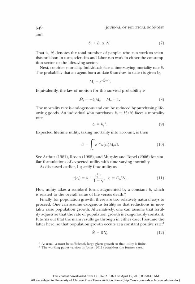
reverse is true for the rates of technological change. That is, gAt is muchfaster than gBt initially. The life sector grows rapidly at first because moreand more people are shifting to work in that sector, not because of fastertechnological change. The relative price of h is therefore actually rising forthe first 130 years of the numerical example, much as it is in the official USdata.Turning now to the long run, notice that the long-run feasible growth

rate of both sectors is �g 5 3:2 percent. The life sector achieves this growthrate in the long run, as does per capita GDP since the life share goes toone. In contrast, the long-run growth rate of the consumption sectoris just 1.3 percent. So this numerical example features a rising growthrate of per capita GDP as the economy shifts toward the life sector buta declining growth rate of ðnonhealthÞ consumption per person.As discussed in Appendix C, other qualitatively different transition dy-

namics are possible in this model, depending on parameter choices. Whatthis numerical example shows is one possibility in which the parameter val-ues are chosen to target a few key moments in the data.

VI. Conclusion

Technological progress involves life and death, and augmenting stan-dard growthmodels to take this into account leads potentially to first-orderchanges in the theory of economic growth. This paper explores these pos-

FIG. 8.—Growth rates along the transition path ðsee fig. 7Þ. Color version available asan online enhancement.


life and growth 567

sibilities, first in a simple “Russian roulette” style model in which new ideascan rarely cause disasters and then in a richer model that features twokinds of ideas, those that increase consumption and those that save lives.The results depend somewhat on the details of the model and, crucially,on how rapidly the marginal utility of consumption declines. It may beoptimal for consumption growth to continue exponentially despite thepresence of life-and-death considerations. Or it may be optimal for con-sumption growth to slow substantially relative to what is feasible, even po-tentially leading to a steady-state level of consumption.The intuition for these results turns out to be straightforward. For a

large class of standard preferences, safety is a luxury good. The marginalutility associated with more consumption on a given day runs into sharpdiminishing returns, and ensuring additional days of life on which to con-sume is a natural, welfare-enhancing response. When the value of life risesfaster than consumption, economic growth leads to a disproportionateconcern for safety. This concern can be so strong that it is desirable thatconsumption growth be restrained.This paper suggests a number of different directions for future re-

search on the economics of safety. It would clearly be desirable to haveprecise estimates of the value of life and how this has changed over time;in particular, does it indeed rise faster than consumption? More empir-ical work on how safety standards have changed over time—and esti-mates of their impacts on economic growth—would also be valuable. Fi-nally, the basic mechanism at work in this paper over time also appliesacross countries. Countries at different levels of income may have verydifferent values of life and therefore different safety standards. This mayhave interesting implications for international trade, standards for pollu-tion and global warming, and international relations more generally.

Appendix A

Derivations and Proofs

This appendix contains outlines of the proofs of the propositions reported inthe paper. As a prelude to these propositions, I first consider the optimal alloca-tion problem in equations ð16Þ–ð21Þ. Using theHamiltonian in ð22Þ and applyingthe maximum principle, the first-order necessary conditions for a solution are

12 stst

5pbt_Bt

pat_At

; ðFOC : sÞ

12 ‘t‘t

5 bdt � vt

u0ðctÞct ; ðFOC : ℓÞ

ðFOC: sÞ

ðFOC: ℓÞ



All

jt

12 jt

5lðp

at_At 1 p

bt_BtÞ

Mt ½u0ðctÞct 1 bdt vt � ; ðFOC : jÞ

r5_vt

vt

11

vt

½uðctÞ2 vtdt �; ðFOC : MÞ

r5_pat

pat

11

pat

Mtu0ðctÞa ct

At

1 patf_At

At

� �; ðFOC : AÞ

r5_pbt

pbt

11

pbt

pbtf_Bt

Bt

1 abvtM t

dt

Bt

� �; ðFOC : BÞ

plus the three standard transversality conditions.It will be convenient, for reasons discussed in the main text, to define

~v t � vt

u0ðctÞct :

This variable denotes the ratio of the value of life to consumption per person.

ðFOC: σ Þ

ðFOC: MÞ

ðFOC: BÞ

ðFOC: AÞ

Proof of Proposition 2: Optimal Growth with γ > 1 1 β

The essence of the result is that the key allocation variables st and ℓt decline ex-ponentially to zero at a constant rate. This exponential shift of scientists towardthe life sector slows the growth rate of consumption ideas. To derive the result, Iuse the various first-order conditions for the optimal allocation.

1. Look back at the first-order condition characterizing the allocation of scien-tists, equation ðFOC: sÞ. To solve for this allocation, we need to solve for the rel-ative price of ideas, p

b=p

a. From equations ðFOC: AÞ and ðFOC: BÞ, we have

pat5

aMtu0ðctÞct=At

r2 gpat2 fg

At

and pbt5

abMtvtdt=Bt

r2 gpbt2 fg

Bt

: ðA1Þ

A condition on the parameter values ðbasically that r is sufficiently largeÞ keepsthe denominators of these expressions positive. This means that the relativeprice satisfies

pbtBt

patAt

5 bdt~v t �r2 g

pat2 fg

At

r2 gpbt2 fg

Bt

: ðA2Þ

This content downloaded from 171.067.216.021 on April 15, 2016 08:50 use subject to University of Chicago Press Terms and Conditions (http://www.journal

:41 AMs.uchicago.edu/t-and-c).

life and growth 569

2. Substituting this expression into ðFOC: sÞ yields

12 stst

5 bdt~v t �r2 g

pat2 fg

At

r2 gpbt2 fg

Bt

� gBtgAt

: ðA3Þ

Recall from ðFOC: ℓÞ that ð12 ‘tÞ=‘t 5 bdt~v t , so both of these key allocation var-iables depend on dt~vt , that is, on the race between the decline in the mortalityrate and the possible rise in the value of life relative to consumption. The nextseveral steps characterize the behavior of dt~vt , which we will then plug back intothis expression.

3. First, consider ~vt . Using ðFOC: MÞ, we obtain

~v t 5uðctÞ=u0ðctÞctr1 dt 2 g

vt

: ðA4Þ

This is a key expression: the value of life in the economy ðas a ratio to con-sumptionÞ depends crucially on the extra utility that person enjoys. The denom-inator essentially converts this flow dividend into a present discounted value.

4. Now recall that given our constant relative risk aversion form for flow utility,

uðctÞu0ðctÞct 5 �ucg21

t 11

12 g:

Since g > 1, along an asymptotic BGP in which ct → ∞,

g ~v 5 ðg2 1Þgc

ðA5Þ

as long as dt converges to some constant.5. Now let us guess that the solution for the asymptotic BGP takes the following

form: st and ℓt fall toward zero at a constant exponential rate, while jt ! j*. Wewill see that the key condition delivering this result will be g > 1 1 b.

6. Under this proposed solution, consumption growth is

gc5 ag

A1 g

‘5 ag

A1 g

s; ðA6Þ

where the last equality comes from observing that along our proposed asymp-totic BGP, g

‘5 g

ssince both st and ℓt are inversely proportional to dt~vt ; see

ðA3Þ above.7. A number of other growth rates follow in a straightforward way from the

various production functions. Most important of these is the growth rate of At.Recall _At 5 slt j

lt N

lt A

f

t and _Bt 5 ð12 stÞljlt N

lt B

ft . The exponential decline in st

will then crucially distinguish the growth rates of At and Bt, since 12 st ! 1 willbe asymptotically constant, while st falls exponentially. Therefore, taking logsand derivatives of these equations, their asymptotic growth rates must satisfy

gA5

lð�n 1 gsÞ12 f

and gB5

l�n

12 f: ðA7Þ



All

8. Combining ðA5Þ, ðA6Þ, and ðA7Þ gives

g ~v 5 ðg2 1Þ alð�n 1 gsÞ

12 f1 g

s

� �: ðA8Þ

9. So to get the growth rate of dt~vt , we now need an expression for gd. Recalldt 5 ½Ba

t ð12 ‘tÞð12 jtÞ�2b. Since 1 2 ℓt converges to one while jt ! j*,

gd52abg

B: ðA9Þ

10. Now, finally, look back at ðA3Þ and consider the asymptotic growth rate ofeach side of the equation. Along our proposed BGP, 1 2 st converges to one, soits growth rate converges to zero. The share st falls exponentially, leading the leftside to grow, while the right side of the equation grows as dt~vt . Using the last tworesults in ðA8Þ and ðA9Þ, taking growth rates of ðA3Þ gives

2gs52abg

B1 ðg2 1Þ alð�n 1 g

sÞ

12 f1 g

s

� �: ðA10Þ

Solving for gs then gives

gs5

2agBðg2 12 bÞ

11 ðg2 1Þ 11al

12 f

� � : ðA11Þ

Under the key assumption that g > 11 b, this solution for gs is negative, as I con-jectured earlier.

11. For completeness, one can also solve for j*, the share of the populationthat becomes scientists. Using ðFOC: jÞ and making some natural substitutions,we find

j*

12 j*5

algB

r2 gpb

2 fgB

;

where, from ðA1Þ, gpb

52ð11 abÞgB. This means that

j*

12 j*5

algB

r1 ð12 f1 abÞgB

: ðA12Þ

Proof of Proposition 3: Optimal Growth with γ < 1 1 β

The first part of the proof follows exactly what we did earlier in proving propo-sition 2. In particular, steps 1–3 are identical.

4. Here things start to change, depending on whether g ≤ 1 or 1 < g < 1 1 b.Notice that

uðctÞu0ðctÞct 5 �ucg21

t 11

12 g:

If g ≤ 1, this ratio ðthe value of a year of life relative to consumptionÞ will con-verge to a constant as ct → ∞, whereas if g > 1, the ratio will grow to infinity. This


life and growth 571

turns out not to matter very much in what follows. In particular, I will focus onthe g > 1 case below, so that

g ~v 5 ðg2 1Þgc: ðA13Þ

ðTo consider the case in which g < 1, simply replace the g2 1 terms below with azero, reflecting the appropriate value of g

~v.Þ

5. Now we can guess that the solution for the asymptotic BGP takes the follow-ing form: ~st � 12 st and ~‘t � 12 ‘t fall toward zero at a constant exponentialrate, while jt → j*. That is, the allocation of scientists and workers shifts awayfrom life and toward the consumption sector.

6. Under this proposed solution, consumption growth is

gc5 ag

AðA14Þ

while growth of the lifesaving aggregate is

g h 5 ag B 1 g ~‘ 5 ag B 1 g ~s : ðA15ÞThe last inequality comes from noting that g ~‘

5 g~s from step 2 in the proof of

proposition 2; see the discussion surrounding equation ðA3Þ above. In fact, itis helpful to repeat that equation here, written in terms of the tilde variables:

~s t12 ~s t

5 bdt~v t �r2 g

pat2 fg

At

r2 gpbt2 fg

Bt

� g Bt

gAt

: ðA16Þ

7. A number of other growth rates follow in a straightforward way from the var-ious production functions. Most important of these is the growth rate of Bt. Re-call _At 5 ð12 ~stÞljl

t Nlt A

f

t and _Bt 5 ~slt jlt N

lt B

ft . The exponential decline in ~st will

then crucially distinguish the growth rates of At and Bt, since 12 ~st ! 1 will beasymptotically constant, while ~st falls exponentially. Therefore, taking logs andderivatives of these equations, their asymptotic growth rates must satisfy

gA 5l�n

12 f and gB 5

lð�n 1 g ~s Þ12 f

: ðA17Þ

8. Combining ðA13Þ, ðA14Þ, and ðA17Þ givesg ~v 5 ðg2 1Þ�g : ðA18Þ

9. So to get the growth rate of dt~vt , we now need an expression for gd. Recalldt 5 ½Ba

t~‘ tð12 jtÞ�2b. Therefore, g

d52bðag

B1 g ~ℓ

Þ. Using this and the fact thatg ~‘

5 g~sgives

gd52b

alð�n 1 g ~s Þ12 f

1 g ~s

� �: ðA19Þ

Combining ðA18Þ and ðA19Þ leads to

gd1 g ~v 52ð11 b2 gÞ�g 2 bg ~s 11

al

12 f

� �: ðA20Þ

10. Now, look back at ðA16Þ and consider the asymptotic growth rate of eachside of the equation. Along our proposed BGP, 12 ~st converges to one, so its



All

growth rate converges to zero. The share ~st falls exponentially, while the rightside of the equation grows with dt~vt . Using our last several results in ðA18Þ,ðA19Þ, and ðA20Þ gives

g ~s 52ðb1 12 gÞ�g 2 bg ~s 11al

12 f

� �: ðA21Þ

Solving for g~s then gives

g ~s 52�g ðb1 12 gÞ

11 b 11al

12 f

� � : ðA22Þ

Under our key assumption that g < 1 1 b, this solution for g~sis negative, as we

conjectured earlier.11. Substituting this result into ðA15Þ then gives the growth rate of the lifesav-

ing aggregate:

g *h 5 �g �

11 ðg 2 1Þ 11al

12 f

� �

11 b 11al

12 f

� �2664

3775 < �g : ðA23Þ

Proof of Proposition 4: Optimal Growth with γ 5 1 1 β

The proof here is straightforward and follows from the earlier proofs. For exam-ple, since g5 11 b, one can see from equation ðA11Þ that gs 5 0. The key growthrates of the economy are then equal to �g immediately.

Appendix B

Data

This appendix describes the construction of the data on the fraction of R&D ex-penditures associated with health. Two separate efforts are made, one using USdata and the other using OECD data. These are discussed in turn.

A. United States

Several main sources are used to construct the US data underlying figure 2. Aspreadsheet available from the data section of my webpage, http://www.stanford.edu/∼chadj/NSF-AllYears -IndustrialRND.xls, contains the detailed calculations.

First, for the years 1971–93, various issues of the NIH Data Book report a timeseries for the key variable in which we are interested: the fraction of R&D relatedto health. In particular, I use the NIH Data Books for 1982, 1989, and 1994, splic-ing together these series during overlapping years to construct the first measureof health R&D. Unfortunately, these data do not appear to be available online, soI used physical copies of the data books.


life and growth 573

The other measures are obtained from a more involved calculation using thefollowing sources:

• Centers for Medicare and Medicaid Services, National Health ExpenditureAccounts, 1960–2009 ðhttps://www.cms.gov/nationalhealthexpenddata/02_nationalhealthaccountshistorical.aspÞ. This data source provides an ex-tensive account of health expenditures, including a “research” category.However, because the purpose is to provide an accounting of health expen-ditures, the research category includes only noncommercial research. Asstated on page 26 of National Health Expenditure Accounts: Definitions, Sources,and Methods 2009, “Research shown separately in the NHEA is that of non-profit or government entities. Research and development expenditures bydrug and medical supply and equipment manufacturers are not shown inthis line, as those expenditures are treated as intermediate purchases underthe definitions of national income accounting; that is, the value of that re-search is deemed to be recouped through product sales.”

• National Science Foundation Industrial Research and Development Infor-mation System data, 1953–98, table H-25 ðhttp://www.nsf.gov/statistics/iris/excel-files/historical_tables/h-25.xlsÞ. From this source, I obtain “Com-pany and Other ðExcept FederalÞ Funds for Industrial R&D Performance,by Industry” for 1953–98. In particular, I sum three industries to get com-mercial health research: “drugs and medicines” ðStandard Industrial Classi-fication [SIC] 283Þ, “health services” ðSIC 80Þ, and then a fraction of “optical,surgical, photographic, and other instruments” ðSIC 384–387Þ. This fractionis equal to 0.569, which is obtained by using the average ratio of health R&Don “medical equipment and supplies” for 1997 and 1998 ðthe two overlap-ping yearsÞ from the next source.

• National Science Foundation, Research and Development in Industryðhttp://www.nsf.gov/statistics/industry/Þ, various issues ð2000, 2002, 2003,2004, 2005Þ. This source reports “Company and Other Nonfederal Fundsfor Industrial R&D Performance” for various years using the North Ameri-can Industry Classification System. I sum three industries to get commercialhealth research: pharmaceuticals and medicines ð3254Þ, medical equip-ment and supplies ð3391Þ, and health care services ð621–623Þ. RaymondWolfe kindly provided the 2006 and 2007 versions of these data.

• Finally, total spending on R&D is obtained from the National Science Foun-dation, National Patterns of R&D Resources: 2008 Data Update ðhttp://www.nsf.gov/statistics/natlpatterns/, which reports data for 1953–2008.

Notice that the measures of commercial/industry R&D exclude federal fundsbut do include nonprofit or state and local funding for R&D. This may result insome double counting. The comparison of the NIH Data Book numbers to thosethat I construct from the NSF sources suggests that this is not a large problem;see figure 2 in the paper.

B. OECD

TheOECD ðand USÞ data underlying figure 3 are taken from the OECD iLibrary.A spreadsheet available from the data section of my webpage, STAN-Health-



All

RND.xls ðhttp://www.stanford.edu/∼chadj/STAN-HealthRND.xlsÞ, contains thedetailed calculations.

Two sets of data from the OECD iLibrary are used:

• Government budget appropriations or outlays for R&D ðhttp://dx.doi.org/10.1787/strd-data-enÞ: This source provides government spending onR&D for health and overall from 1981 to 2007 in current purchasing powerparity adjusted US dollars.

• STANR&DExpenditure in Industry ðISIC Rev. 3ÞANBERD ed2009 ðhttp://stats.oecd.org/Index.aspx?DataSetCode5ANBERD_REV3Þ: This source pro-vides spending on R&D by industry. Because of a relatively limited indus-try breakdown, the health measure is the sum of spending in the phar-maceutical industry ðC2423Þ and 0.5 times the spending in the “medical,precision, and optical instruments” industry ðC33Þ; this weight of 0.5 is ob-viously arbitrary but was suggested by calculations using the US sources dis-cussed earlier.

From these data, I calculate the health share of R&D for both the UnitedStates and a set of OECD countries. For government R&D, the OECD aggregateincludes the United States, the United Kingdom, France, Germany, Italy, Japan,and Canada. For some reason, the industry data for France and the United King-dom are not available, so these countries are not included in the industry com-ponent.

Appendix C

Solving the Model Numerically

The transition dynamics of the optimal allocation can be studied as a system ofsix differential equations in six “state-like” variables that converge to constant val-ues: st, ℓt, jt, dt, yt, and zt. These variables, their meaning, and their steady-state val-ues are displayed in table C1.

Letting a “hat” denote a growth rate, the laws of motion for these state-like var-iables are

TABLE C1Key Variables for Studying Transition Dynamics

Variable Meaning Steady-State Value

st Share of scientists in the consumption sector s* 5 0ℓt Share of workers in the consumption sector ℓ

* 5 0jt Scientists’ share of the population j* 5

algB

r1ð12f1abÞg B

dt Mortality rate d* 5 0yt ; gAt Growth rate of At y* 5 gAzt ; gBt Growth rate of Bt z* 5 gB

This con use subject to Unive

tent downloaded from 171.067.216.021 on April 15, 201rsity of Chicago Press Terms and Conditions (http://www

6 08:50:41 AM.journals.uchicago.edu/t-and-c).

life and growth 575

s 5 azð12 ‘Þ l

12 l� 12 j

j12

‘

12 ‘� 12 s

s� yz

� �;

‘ 5v‘ð① 1 vjqÞ12 qgvj

;

j 5 vjð ② 1 g‘Þ;

d 5 2abz 1 b‘ � ‘

12 ‘1 bj � j

12 j;

y 5 lð�n 1 s 1 jÞ2 ð12 fÞy;z 5 l �n 2 s � s

12 s1 j

� �2 ð12 fÞy;

where the following definitions have been used:

v‘ 512 ‘

g2 ðg2 12 bÞ‘ ;

vj 51

12 l1gj

12 j

;

① 5 abz 1 bd~u � ‘

12 ‘2 r2 d2 ðg2 1Þay;

② 5 r1 d1 ð12 lÞs � s

12 sl�n 1 ðg2 1Þay 2 alzð12 ‘Þ

12 s� 12 j

j:

I solve the system of differential equations using “reverse shooting”; seeJudd ð1998, 355Þ. That is, I start from the steady state, consider a small devia-tion, and then run time backward. To determine parameter values, I proceededas follows.

1. To get the deviation from the steady state, I first select a mortality rate dT ðIend up choosing dT 5 .0002Þ.

2. Next, I find the values of sT and ℓT that minimize the distance between s T , ‘T ,and jT from their BGP values—gs for the first two and zero for j.

3. Given choices for the parameter values, I can then use the reverse shootingmethod to get a candidate path.

4. I use “fminsearch” in Matlab to find values for �u, b, g, and l that minimizethe weighted sum of squared deviations between a selection of moments and aset of preferred values. These moments and values are given below:

a. Given a candidate path, we first find the year t * such that ~uðt *Þ is the closestto 3.5. That is, we find the year in which the value of a year of life as a ratioto consumption is closest to 3.5. This corresponds, for example, to a valueof a year of life of $125,000 and a consumption per person of $36,000,roughly consistent with the United States today.

b. Our first moment is ~uðt*Þ compared to 3.5.c. Our secondmoment is sðt *Þ compared to 75 percent, motivated by figure 2,

suggesting that around 25 percent of research is for health.



All

d. Our final moment is the growth rate of GDP in the year t *, for which thetarget value is 2 percent.

5. Depending on the initial guess for these parameter values, this process findsdifferent “local” optima, in part because the year t * is free to move around. Ichanged the weights on the various moments and also considered different valuesof f from the set f1/4, 1/2, 3/4, 5/6g to hunt for the best overall fit. The resultsreported in the main text use the following parameter values: g 5 2.6953, b 50.6006, �u 5 :001, l 5 .5377, dT 5 .0002, f 5 5/6, r 5 .02, and a 5 1.

6. In general, two kinds of results emerged from this exercise. The first is whatis shown in the main text, where the growth rate of A falls while the growth rateof B rises. For values of f other than 5/6, one often finds values of sðt *Þ that werevery close to one rather than close to 0.75. The other main dynamic that I foundfeatured growth rates of A and B that started near zero and then rose over time.In these results, it was easy to get sðt*Þ ≈ 0:75 but was hard to get GDP growtharound 2 percent in the same year.

References

Acemoglu, Daron. 2002. “Directed Technical Change.” Rev. Econ. Studies 69 ð4Þ:781–810.

Acemoglu, Daron, Amy Finkelstein, andMatthew J. Notowidigdo. 2009. “Incomeand Health Spending: Evidence from Oil Price Shocks.” Working paper, Mas-sachusetts Inst. Tech.

Acemoglu, Daron, and Simon Johnson. 2007. “Disease and Development: TheEffect of Life Expectancy on Economic Growth.” J.P.E. 115 ð6Þ: 925–85.

Aghion, Philippe, and Peter Howitt. 1992. “A Model of Growth through CreativeDestruction.” Econometrica 60 ð2Þ: 323–51.

Arthur, W. B. 1981. “The Economics of Risk to Life.” A.E.R. 71 ð1Þ: 54–64.Ashenfelter, Orley, andMichael Greenstone. 2004. “Using Mandated Speed Lim-

its to Measure the Value of a Statistical Life.” J.P.E. 112, no. 1, pt. 2 ðFebruaryÞ:S226–S267.

Attanasio, Orazio P., and Guglielmo Weber. 1995. “Is Consumption Growth Con-sistent with Intertemporal Optimization? Evidence from the Consumer Ex-penditure Survey.” J.P.E. 103 ð6Þ: 1121–57.

Barsky, R. B., F. T. Juster, M. S. Kimball, and M. D. Shapiro. 1997. “Preference Pa-rameters and Behavioral Heterogeneity: An Experimental Approach in theHealth and Retirement Study.” Q.J.E. 112 ð2Þ: 537–79.

Becker, Gary S., Tomas J. Philipson, and Rodrigo R. Soares. 2005. “The Quantityand Quality of Life and the Evolution of World Inequality.” A.E.R. 95 ð1Þ: 277–91.

Berndt, Ernst R., Anupa Bir, Susan H. Busch, Richard G. Frank, and Shaon-LiseT. Normand. 2000. “The Medical Treatment of Depression, 1991–1996: Pro-ductive Inefficiency, Expected Outcome Variations, and Price Indexes.”Work-ing Paper no. 7816, NBER, Cambridge, MA.

Brock, William, and M. Scott Taylor. 2005. “Economic Growth Theory and theEnvironment: A Review of Theory and Empirics.” In Handbook of EconomicGrowth, edited by Philippe Aghion and Steven N. Durlauf, 1749–1821. Amster-dam: Elsevier.


http://www.journals.uchicago.edu/action/showLinks?crossref=10.1162%2F003355397555280

http://www.journals.uchicago.edu/action/showLinks?system=10.1086%2F529000



http://www.journals.uchicago.edu/action/showLinks?crossref=10.1111%2F1467-937X.00226

life and growth 577

Chetty, Raj. 2006. “A New Method of Estimating Risk Aversion.” A.E.R. 96 ð5Þ:1821–34.

Clemens, Jeffrey P. 2013. “The Effect of U.S. Health Insurance Expansions onMedical Innovation.” Technical report, Univ. California, San Diego.

Costa, Dora L., and Matthew E. Kahn. 2004. “Changes in the Value of Life, 1940–1980.” J. Risk and Uncertainty 29 ð2Þ: 159–80.

Cutler, David M., Mark B. McClellan, Joseph P. Newhouse, and Dahlia Remler.1998. “Are Medical Prices Declining? Evidence from Heart Attack Treat-ments.” Q.J.E. 113 ð4Þ: 991–1024.

Dalgaard, Carl-Johan, and Holger Strulik. 2014. “Optimal Aging and Death: Un-derstanding the Preston Curve.” J. European Econ. Assoc. 12 ð3Þ: 672–701.

Ehrlich, Isaac, and Hiroyuki Chuma. 1990. “A Model of the Demand for Longev-ity and the Value of Life Extension.” J.P.E. 98 ð4Þ: 761–82.

Griliches, Zvi. 1990. “Patent Statistics as Economic Indicators: A Survey.” J. Econ.Literature 28 ð4Þ: 1661–1707.

Grossman, Michael. 1972. “On the Concept of Health Capital and the Demandfor Health.” J.P.E. 80 ð2Þ: 223–55.

Gruber, Jonathan. 2006. “ATax-Based Estimate of the Elasticity of IntertemporalSubstitution.” Working Paper no. 11945, NBER, Cambridge, MA.

Guvenen, Fatih. 2006. “Reconciling Conflicting Evidence on the Elasticity ofIntertemporal Substitution: A Macroeconomic Perspective.” J. Monetary Econ.53 ð7Þ: 1451–72.

Hall, Robert E. 1988. “Intertemporal Substitution in Consumption.” J.P.E. 96 ð2Þ:339–57.

———. 2009. “Reconciling Cyclical Movements in the Marginal Value of Timeand the Marginal Product of Labor.” J.P.E. 117 ð2Þ: 281–323.

Hall, Robert E., and Charles I. Jones. 2007. “The Value of Life and the Rise inHealth Spending.” Q.J.E. 122 ð1Þ: 39–72.

Hammitt, James K., Jin-Tan Liu, and Jin-Long Liu. 2000. “Survival Is a LuxuryGood: The Increasing Value of a Statistical Life.” Manuscript, Harvard Univ.

Jones, Charles I. 1995. “R&D-Based Models of Economic Growth.” J.P.E. 103 ð4Þ:759–84.

———. 2011. “Life and Growth.” Working Paper no. 17094, NBER, Cambridge,MA.

Jones, Charles I., and Paul M. Romer. 2010. “The New Kaldor Facts: Ideas, Insti-tutions, Population, and Human Capital.” American Econ. J.: Macroeconomics 2ð1Þ: 224–45.

Judd, Kenneth L. 1998. Numerical Methods in Economics. Cambridge, MA: MITPress.

Lawver, Daniel. 2011. “Measuring Quality Increases in the Medical Sector.”Man-uscript, Arizona State Univ.

Lucas, Deborah. 1994. “Asset Pricing with Undiversifiable Risk and Short SalesConstraints: Deepening the Equity Premium Puzzle.” J. Monetary Econ. 34 ð3Þ:325–42.

Malani, Anup, and Tomas J. Philipson. 2011. “Can Medical Progress Be Sus-tained? Implications of the Link between Development and Output Markets.”Working Paper no. 17011, NBER, Cambridge, MA.

Murphy, Kevin M., and Robert Topel. 2003. “The Economic Value of Medical Re-search.” In Measuring the Gains from Medical Research: An Economic Approach, ed-ited by Kevin M. Murphy and Robert Topel, 41–73. Chicago: Univ. ChicagoPress.

———. 2006. “The Value of Health and Longevity.” J.P.E. 114 ð5Þ: 871–904.





http://www.journals.uchicago.edu/action/showLinks?crossref=10.1162%2Fqjec.122.1.39



http://www.journals.uchicago.edu/action/showLinks?crossref=10.1111%2Fjeea.12071

http://www.journals.uchicago.edu/action/showLinks?crossref=10.1016%2F0304-3932%2894%2990022-1

http://www.journals.uchicago.edu/action/showLinks?crossref=10.1016%2Fj.jmoneco.2005.06.001

http://www.journals.uchicago.edu/action/showLinks?crossref=10.1016%2Fj.jmoneco.2005.06.001

http://www.journals.uchicago.edu/action/showLinks?crossref=10.1257%2Fmac.2.1.224

http://www.journals.uchicago.edu/action/showLinks?crossref=10.1257%2Fmac.2.1.224


http://www.journals.uchicago.edu/action/showLinks?crossref=10.1023%2FB%3ARISK.0000038942.18349.88



All

Nordhaus, William D. 2003. “The Health of Nations: The Contribution of Im-proved Health to Living Standards.” In Measuring the Gains from Medical Re-search: An Economic Approach, edited by Kevin M. Murphy and Robert Topel,9–40. Chicago: Univ. Chicago Press.

Romer, Paul M. 1986. “Cake Eating, Chattering, and Jumps: Existence Results forVariational Problems.” Econometrica 54:897–908.

———. 1990. “Endogenous Technological Change.” J.P.E. 98, no. 5, pt. 2 ðOcto-berÞ: S71–S102.

Rosen, Sherwin. 1988. “The Value of Changes in Life Expectancy.” J. Risk and Un-certainty 1:285–304.

Shapiro, Irving, Matthew D. Shapiro, and David W. Wilcox. 1999. “Measuring theValue of Cataract Surgery.” Manuscript, Univ. Michigan.

Stokey, Nancy L. 1998. “Are There Limits to Growth?” Internat. Econ. Rev. 39:1–31.

Triplett, Jack E., and Barry P. Bosworth. 2000. “Productivity in the Services Sec-tor.” Manuscript, Brookings Inst., Washington, DC.

Viscusi, W. Kip, and Joseph E. Aldy. 2003. “The Value of a Statistical Life: A Crit-ical Review of Market Estimates throughout the World.” J. Risk and Uncertainty27:5–76.

Vissing-Jorgensen, Annette, and Orazio P. Attanasio. 2003. “Stock-Market Partic-ipation, Intertemporal Substitution, and Risk-Aversion.” A.E.R. Papers andProc. 93 ð2Þ: 383–91.

Weisbrod, Burton A. 1991. “The Health Care Quadrilemma: An Essay on Tech-nological Change, Insurance, Quality of Care, and Cost Containment.” J. Econ.Literature 29:523–52.



http://www.journals.uchicago.edu/action/showLinks?crossref=10.1023%2FA%3A1025598106257


http://www.journals.uchicago.edu/action/showLinks?crossref=10.1007%2FBF00056139

http://www.journals.uchicago.edu/action/showLinks?crossref=10.1007%2FBF00056139


Life and Growth - Stanford Universityweb.stanford.edu/~chadj/LifeandGrowthJPE2016.pdf · Life and...

Documents

Transcript of Life and Growth - Stanford Universityweb.stanford.edu/~chadj/LifeandGrowthJPE2016.pdf · Life and...