1

Life After the EM Algorithm: The Variational Approximation for Bayesian Inference.

Dimitris Tzikas, Aristidis Likas, Senior Member, IEEE

and Nikolaos Galatsanos, Senior Member, IEEE

Department of Computer Science, University of Ioannina

GR 45110, Ioannina, Greece

{tzikas, arly, galatsanos}@cs.uoi.gr

Thomas Bayes (1701-1761), shown in the upper left, first discovered “Bayes’ theorem” in a paper that was published in 1764 three years after his death, as the name suggests. However, Bayes in his theorem used uniform priors [1] and [2]. Pierre-Simon Laplace (1749-1827), shown in the lower right, unaware of Bayes’ work, discovered the same theorem in its general form in a memoir he wrote at the age of 25. In this memoir he also introduced “Bayesian Inference” to statistics [2]. Regarding these issues S. M. Stiegler writes in [3] “The influence of this memoir was immense. It was from here that “Bayesian” ideas first spread through the mathematical world, as Bayes’s own article was ignored until 1780 and played no important role in scientific debate until the twentieth century. It was also this article of Laplace’s that introduced the mathematical techniques for the asymptotic analysis of posterior distributions that are still employed today. And it was here that the earliest example of optimum estimation can be found, the derivation and characterization of an estimator that minimized a particular measure of posterior expected loss. After more than two centuries, we mathematicians, statisticians cannot only recognize our roots in this masterpiece of our science, we can still learn from it.”

2

Abstract

Maximum Likelihood (ML) estimation is one of the most popular methodologies

used in modern statistical signal processing. The Expectation Maximization (EM) algorithm

is an iterative algorithm for ML estimation that has a number of advantages and has become a

standard methodology for solving statistical signal processing problems. However, the EM

has certain requirements that seriously limit its applicability to complex problems. Recently, a

new methodology termed “variational Bayesian inference” has emerged, which relaxes some

of the limiting requirements of the EM algorithm and is gaining rapidly popularity.

Furthermore, one can show that the EM algorithm can be viewed as a special case of this

methodology. In this paper we first present a tutorial introduction of Bayesian variational

inference aimed at the signal processing community. Then, we use linear regression and

Gaussian mixture modeling as examples to demonstrate the additional capabilities that

Bayesian variational inference offers as compared to the EM algorithm.

1. Introduction

The maximum likelihood (ML) methodology is one of the basic staples of modern

statistical signal processing. The expectation-maximization (EM) algorithm is an iterative

algorithm that offers a number of advantages for obtaining ML estimates. Since its formal

introduction in 1977 by Dempster et al. [4], the EM algorithm has become a standard

methodology for ML estimation. In the IEEE community, the EM is steadily gaining

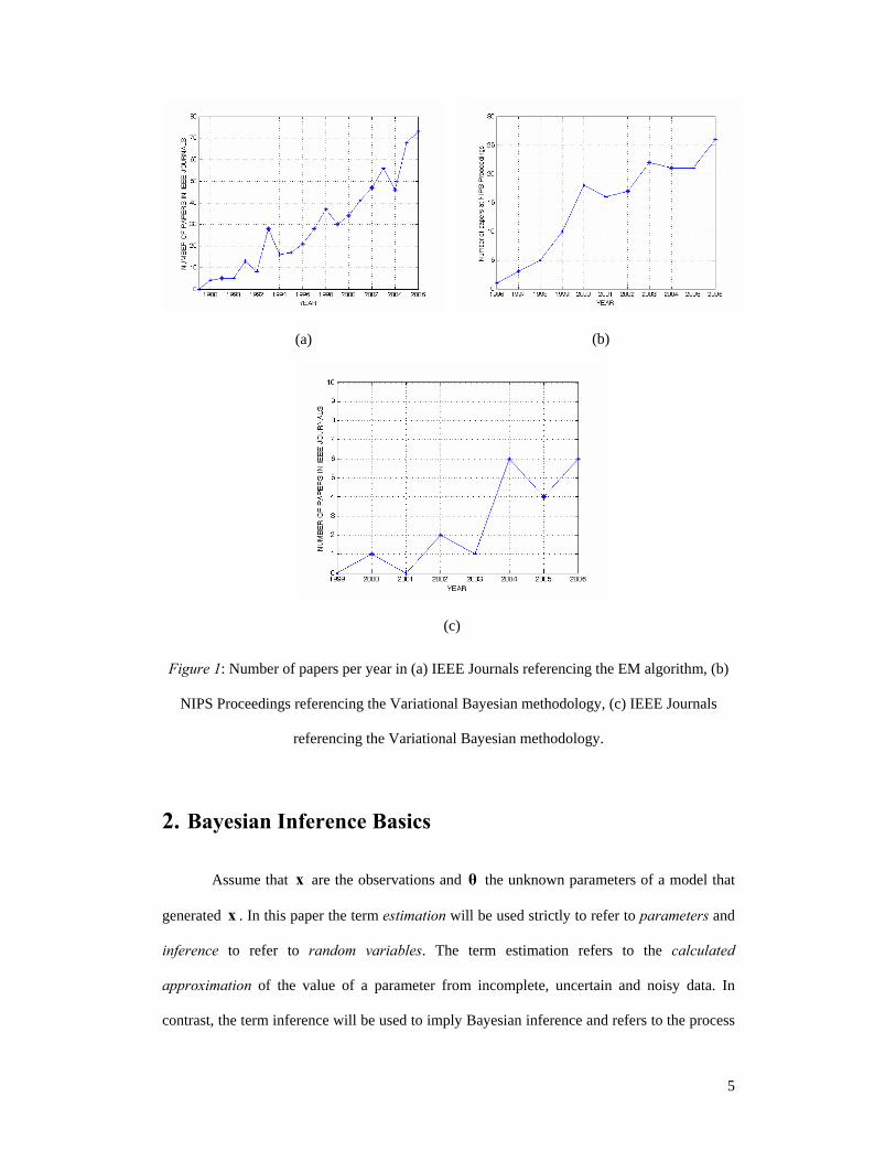
popularity and is being used in an increasing number of applications. To substantiate this

point in Figure 1(a) we show the number of IEEE journal papers per year1 for the period

1988-2006 which refer to the EM algorithm. In this figure we observe an almost exponential

growth during this time period. The first publications in IEEE journals making reference to

the EM algorithm appeared in 1988 and dealt with the problem of tomographic reconstruction

3

of photon limited images [5] and [6]. Since then, the EM algorithm has become a popular tool

for statistical signal processing used in a wide range of applications, such as recovery and

segmentation of images and video, image modelling, carrier frequency synchronization,

channel estimation in communications and speech recognition.

The concept behind the EM algorithm is very intuitive and natural. EM-like

algorithms existed in the statistical literature even before [4], however such algorithms were

actually EM algorithms in special contexts. The first known such reference dates back to

1886. There Newcomb considers the estimation of the parameters of a mixture of two

univariate normals [7]. However, it was in [4] where such ideas were synthesized and the

general formulation of the EM algorithm was established. A good survey on the history of the

EM algorithm before [4] can be found in [8].

The present article is not a tutorial on the EM algorithm. Such a tutorial appeared in

1996 in the Signal Processing Magazine [9]. The present article is aimed at presenting an

emerging new methodology for Statistical Inference which ameliorates certain shortcomings

of the EM. This methodology is termed Variational Approximation and can be used to solve

complex Bayesian models where the EM algorithm cannot be applied. Bayesian Inference

based on the Variational approximation has been used extensively by the Machine Learning

community since the mid 90 when it was first introduced. As an indication of this, in Figure

1(b) we show the number of papers per year at the Proceedings of Neural Information

Processing Systems (NIPS) conference (one of the flagship conferences of this community),

that use the Variational methodology from 1996, when the first such paper [12] appeared, till

2006.

In the IEEE community recently there is a budding interest in this methodology [28].

To get a better feeling for this, Figure 1(c) shows the number of IEEE journal papers per

year2 that use the Variational Bayesian methodology from 2000, when the first such paper

[11] appeared, till 2006. Comparing Figures 1(a) and 1(c) one could say that in terms of trend

1 From IEEE Xplore 2 From IEEE Xplore

4

line the present status of the Variational methodology is reminiscent to the status of the EM

algorithm in the early 90s. To our knowledge this methodology has been already been applied

to certain signal processing applications. For example, it has been applied to speech

processing problems [31], [32], and [33], inverse problems in imaging; [17], [37], [36], [38],

and [39], and processing of biomedical signals [34] and [35].

The objective of this tutorial is to help popularize this methodology within the IEEE

Signal Processing community. The rest of this tutorial paper is organized as follows: in

Section 2 we introduce some basic concepts of Bayesian Inference. In Section 3 we present

Graphical Models, a convenient tool for visualizing Bayesian models. In Section 4 we present

the EM algorithm from a perspective that allows its subsequent generalization which is

presented in Section 5 termed Variational EM. In Section 6 we use three different Linear

Regression (LR) models as examples to demonstrate the theory in Sections 4 and 5. In

Section 7 we use Gaussian Mixture Models (GMM) as another example to the previous

theory. Finally, in Section 8 we present our concluding remarks. Also in Appendix-A of this

tutorial paper we introduce MAP estimation and we show how a MAP-EM algorithm can be

derived and in Appendix-B we discuss why Bayesian inferenc is tractable when using

conjugate prior distributions.

5

Figure 1: Number of papers per year in (a) IEEE Journals referencing the EM algorithm, (b)

NIPS Proceedings referencing the Variational Bayesian methodology, (c) IEEE Journals

referencing the Variational Bayesian methodology.

2. Bayesian Inference Basics

Assume that x are the observations and θ the unknown parameters of a model that

generated x . In this paper the term estimation will be used strictly to refer to parameters and

inference to refer to random variables. The term estimation refers to the calculated

approximation of the value of a parameter from incomplete, uncertain and noisy data. In

contrast, the term inference will be used to imply Bayesian inference and refers to the process

(a)

(b)

(c)

6

in which prior evidence and observations are used to infer the posterior probability ( )p |θ x

of the random variables θ given the observations x .

One of the most popular approaches for parameter estimation is maximum likelihood

(ML). According to this approach, the ML estimate is obtained as

ˆ arg max ( )ML p= ;θ

x θθ . (2.1)

where ( )p ;x θ describes the probabilistic relationship between the observations and the

parameters based on the assumed model that generated the observations x . At this point we

would like to clarify the difference between the notation ( )p ;x θ and ( )p |x θ . When we

write ( )p ;x θ we imply that θ are parameters and as a function of θ is called the likelihood

function. In contrast, when we write ( )p |x θ we imply that θ are random variables.

In many cases of interest direct assessment of the likelihood function ( )p ;x θ is

complex and is either difficult or impossible to compute it directly or optimize it. In such

cases the computation of this likelihood is greatly facilitated by the introduction of hidden

variables z . These random variables act as “links” that connect the observations to the

unknown parameters via Bayes’ law. The choice of hidden variables is problem dependent.

However, as their name suggests, these variables are not observed and they provide enough

information about the observations so that the conditional probability ( )p |x z is easy to

compute. Apart from this role, hidden variables play another role in statistical modelling.

They are an important part of the probabilistic mechanism that is assumed to have generated

the observations and can be described very succinctly by a graph that is termed “graphical

model”. More details on graphical models is given in Section 3.

Once hidden variables and a prior probability for them ( )p ;z θ have been introduced,

one can obtain the likelihood or the marginal likelihood as it is called at times by integrating

out (marginalizing) the hidden variables according to

( ) ( ) ( ) ( )p p d p p d; = , ; = | ; ;∫ ∫x θ x z θ z x z θ z θ z . (2.2)

This seemingly simple integration is the crux of the Bayesian methodology because

7

in this manner we can obtain both the likelihood function, and by using Bayes’ theorem, the

posterior of the hidden variables according to

( ) ( ) ( )( )

|;

p pp

p| ; ;

; =x z θ z θ

z x θx θ

. (2.3)

Once the posterior is available, inference as explained above for the hidden variables is also

possible. Despite the simplicity of the above formulation, in most cases of interest the integral

in Eq. (2.2) is either impossible or very difficult to compute in closed form. Thus, the main

effort in Bayesian Inference is concentrated on techniques that allow us to bypass or

approximately evaluate this integral.

Such methods can be classified into two broad categories. The first is numerical

sampling methods also known as Monte Carlo techniques and the second is deterministic

approximations. This paper will not address at all Monte Carlo methods. The interested reader

for such methods is referred to a number of books and survey articles on this topic, for

example [10] and [11].

As it will be shown in what follows, the EM algorithm is a Bayesian inference

methodology that assumes knowledge of the posterior ( )|p ;z x θ and iteratively maximizes

the likelihood function without explicitly computing it. A serious shortcoming of this

methodology is that in many cases of interest this posterior is not available. However, recent

developments in Bayesian inference allow us to bypass this difficulty by approximating the

posterior. They are termed “Variational Bayesian” and they will be the focus of this tutorial.

3. Graphical Models

Graphical Models provide a framework for representing dependencies among the

random variables of a statistical modelling problem and they constitute a comprehensive and

elegant way to graphically represent the interaction among the entities involved in a

probabilistic system. A graphical model is a graph whose nodes correspond to the random

variables of a problem and the edges represent the dependencies among the variables. A

8

directed edge from a node A to a node B in the graph denotes that the variable B stochastically

depends on the value of the variable A. Graphical models can be either directed or undirected.

In the second case they are also known as Markov Random Fields [11], [24] and [25]. In the

rest of this tutorial, we will focus on directed graphical models also called Bayesian

Networks, where all the edges are considered to have a direction from parent to child denoting

the conditional dependency among the corresponding random variables. In addition we

assume that the directed graph is acyclic (i.e. contains no cycles).

Let ( ),G V E= be a directed acyclic graph with V being the set of nodes and E the

set of directed edges. Let also sx denote the random variable associated with node s and

( )sπ the set of parents of node s . Associated with each node s is also a conditional

probability density ( )( )|s sp x xπ that defines the distribution of sx given the values of its

parent variables. Therefore, for a graphical model to be completely defined, apart from the

graph structure, the conditional probability distribution at each node should also be specified.

Once these distributions are known, the joint distribution over the set of all variables can be

computed as the product:

( ) ( )( )| .s ss

p x p x xπ=∏ (3.1)

The above equation constitutes a formal definition of a directed graphical model [13] as a

collection of probability distributions that factorize in the way specified in the above equation

(which of course depends on the structure of the underlying graph).

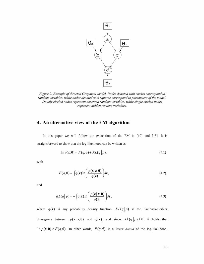
In Figure 2 we show an example of a directed Graphical Model. The random

variables depicted at the nodes are a,b,c and d. Each node represents a conditional probability

density that quantifies the dependency of the node from its parents. The densities at the nodes

might not be exactly known and can be parameterized by a set of parameters iθ . Using the

chain rule of probability we would write the joint distribution as:

( ) ( ) ( ) ( ) ( )1 2 3 4, , , ; ; ; | , ; , , ; .p a b c d p a p b a p c a b p d a b cθ θ θ θ=θ (3.2)

9

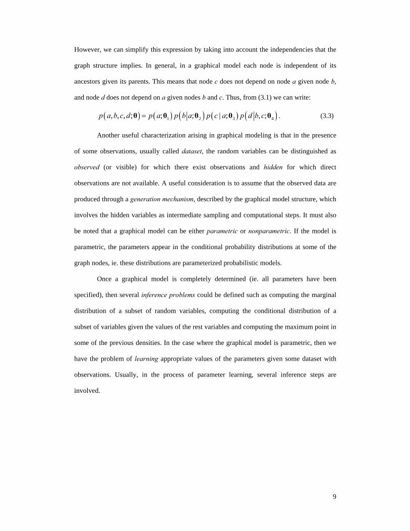
However, we can simplify this expression by taking into account the independencies that the

graph structure implies. In general, in a graphical model each node is independent of its

ancestors given its parents. This means that node c does not depend on node a given node b,

and node d does not depend on a given nodes b and c. Thus, from (3.1) we can write:

( ) ( ) ( ) ( ) ( )1 2 3 4, , , ; ; ; | ; , ;p a b c d p a p b a p c a p d b c=θ θ θ θ θ . (3.3)

Another useful characterization arising in graphical modeling is that in the presence

of some observations, usually called dataset, the random variables can be distinguished as

observed (or visible) for which there exist observations and hidden for which direct

observations are not available. A useful consideration is to assume that the observed data are

produced through a generation mechanism, described by the graphical model structure, which

involves the hidden variables as intermediate sampling and computational steps. It must also

be noted that a graphical model can be either parametric or nonparametric. If the model is

parametric, the parameters appear in the conditional probability distributions at some of the

graph nodes, ie. these distributions are parameterized probabilistic models.

Once a graphical model is completely determined (ie. all parameters have been

specified), then several inference problems could be defined such as computing the marginal

distribution of a subset of random variables, computing the conditional distribution of a

subset of variables given the values of the rest variables and computing the maximum point in

some of the previous densities. In the case where the graphical model is parametric, then we

have the problem of learning appropriate values of the parameters given some dataset with

observations. Usually, in the process of parameter learning, several inference steps are

involved.

10

Figure 2: Example of directed Graphical Model. Nodes denoted with circles correspond to random variables, while nodes denoted with squares correspond to parameters of the model.

Doubly circled nodes represent observed random variables, while single circled nodes represent hidden random variables.

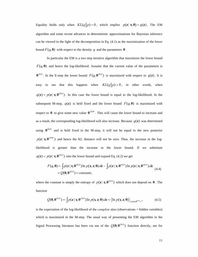
4. An alternative view of the EM algorithm

In this paper we will follow the exposition of the EM in [10] and [13]. It is

straightforward to show that the log-likelihood can be written as

ln ( ) ( ) ( )p F q KL q p; = , +x θ θ , (4.1)

with

( )( ) ( ) ln

( )pF q q d

q⎛ ⎞, ;

, = ⎜ ⎟⎝ ⎠

∫x z θθ z z

z, (4.2)

and

( )( ) ( ) ln

( )pKL q p q d

q⎛ ⎞| ;

= − ⎜ ⎟⎝ ⎠

∫z x θz z

z, (4.3)

where ( )q z is any probability density function. ( )KL q p is the Kullback-Leibler

divergence between ( )p | ;z x θ and ( )q z , and since ( ) 0KL q p ≥ , it holds that

ln ( ) ( )p F q; ≥ ,x θ θ . In other words, ( )F q θ, is a lower bound of the log-likelihood.

11

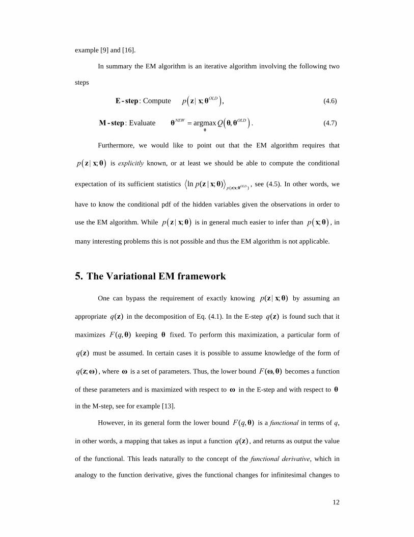
Equality holds only when ( ) 0KL q p = , which implies ( ) ( )p q| ; =z x θ z . The EM

algorithm and some recent advances in deterministic approximations for Bayesian inference

can be viewed in the light of the decomposition in Eq. (4.1) as the maximization of the lower

bound ( )F q,θ with respect to the density q and the parameters θ .

In particular the EM is a two step iterative algorithm that maximizes the lower bound

( )F q,θ and hence the log-likelihood. Assume that the current value of the parameters is

OLDθ . In the E-step the lower bound ( )OLDF q,θ is maximized with respect to ( )q z . It is

easy to see that this happens when ( ) 0KL q p = , in other words, when

( ) ( )OLDq p= | ;z z x θ . In this case the lower bound is equal to the log-likelihood. In the

subsequent M-step, ( )q z is held fixed and the lower bound ( )F q,θ is maximized with

respect to θ to give some new value NEWθ . This will cause the lower bound to increase and

as a result, the corresponding log-likelihood will also increase. Because ( )q z was determined

using OLDθ and is held fixed in the M-step, it will not be equal to the new posterior

( )NEWp | ;z x θ and hence the KL distance will not be zero. Thus, the increase in the log-

likelihood is greater than the increase in the lower bound. If we substitute

( ) ( )OLDq p= | ;z z x θ into the lower bound and expand Eq. (4.2) we get

( ) ( | ) ln ( ) ( | ) ln ( | )

( ) ,

OLD OLD OLD

OLD

F q p p d p p d

Q constant

, = ; , ; − ; ;

= , +∫ ∫θ z x θ x z θ z z x θ z x θ z

θ θ (4.4)

where the constant is simply the entropy of ( )OLDp | ;z x θ which does not depend on θ . The

function

( | )( ) ( | ) ln ( ) ln ( ) ,OLD

OLD OLDp

Q p p d p;

, = ; , ; = , ;∫ z x θθ θ z x θ x z θ z x z θ (4.5)

is the expectation of the log-likelihood of the complete data (observations + hidden variables)

which is maximized in the M-step. The usual way of presenting the EM algorithm in the

Signal Processing literature has been via use of the ( )OLDQ ,θ θ function directly, see for

12

example [9] and [16].

In summary the EM algorithm is an iterative algorithm involving the following two

steps

( )Compute ,OLDp: | ;E - step z x θ (4.6)

( )Evaluate argmaxNEW OLDQ: = ,θ

M - step θ θ θ . (4.7)

Furthermore, we would like to point out that the EM algorithm requires that

( )p | ;z x θ is explicitly known, or at least we should be able to compute the conditional

expectation of its sufficient statistics ( | )

ln ( | ) OLDpp

;;

z x θz x θ , see (4.5). In other words, we

have to know the conditional pdf of the hidden variables given the observations in order to

use the EM algorithm. While ( )p | ;z x θ is in general much easier to infer than ( )p ;x θ , in

many interesting problems this is not possible and thus the EM algorithm is not applicable.

5. The Variational EM framework

One can bypass the requirement of exactly knowing ( )p | ;z x θ by assuming an

appropriate ( )q z in the decomposition of Eq. (4.1). In the E-step ( )q z is found such that it

maximizes ( )F q,θ keeping θ fixed. To perform this maximization, a particular form of

( )q z must be assumed. In certain cases it is possible to assume knowledge of the form of

( )q ;z ω , where ω is a set of parameters. Thus, the lower bound ( )F ,ω θ becomes a function

of these parameters and is maximized with respect to ω in the E-step and with respect to θ

in the M-step, see for example [13].

However, in its general form the lower bound ( )F q,θ is a functional in terms of q,

in other words, a mapping that takes as input a function ( )q z , and returns as output the value

of the functional. This leads naturally to the concept of the functional derivative, which in

analogy to the function derivative, gives the functional changes for infinitesimal changes to

13

the input function. This area of mathematics is called calculus of variations [18] and has been

applied to many areas of mathematics, physical sciences and engineering, for example fluid

mechanics, heat transfer and control theory to name a few.

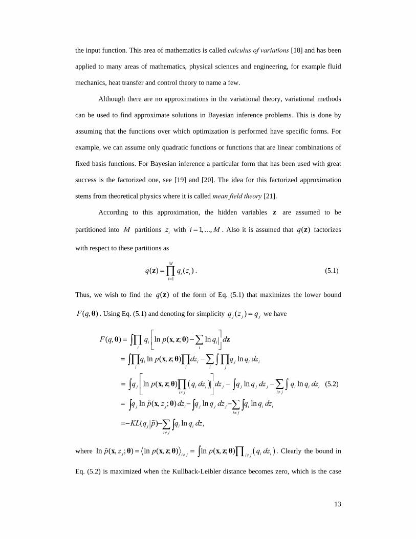
Although there are no approximations in the variational theory, variational methods

can be used to find approximate solutions in Bayesian inference problems. This is done by

assuming that the functions over which optimization is performed have specific forms. For

example, we can assume only quadratic functions or functions that are linear combinations of

fixed basis functions. For Bayesian inference a particular form that has been used with great

success is the factorized one, see [19] and [20]. The idea for this factorized approximation

stems from theoretical physics where it is called mean field theory [21].

According to this approximation, the hidden variables z are assumed to be

partitioned into M partitions iz with 1 ,i … M= , . Also it is assumed that ( )q z factorizes

with respect to these partitions as

1

( ) ( )M

i ii

q q z=

=∏z . (5.1)

Thus, we wish to find the ( )q z of the form of Eq. (5.1) that maximizes the lower bound

( )F q,θ . Using Eq. (5.1) and denoting for simplicity ( )j j jq z q= we have

( )

( ) ln ( ) ln

ln ( ) ln

ln ( ) ln ln

ln ( ) ln ln

( ) ln

i iii

i i j i iii i j

j i i j j j j i i ii ji j

j j i j j j i i ii j

i iji j

F q q p q d

q p dz q q dz

q p q dz dz q q dz q q dz

q p z dz q q dz q q dz

KL q p q q dz

≠≠

≠

≠

⎡ ⎤, = , ; −⎢ ⎥⎣ ⎦

= , ; −

⎡ ⎤= , ; − −⎢ ⎥

⎣ ⎦= , ; − −

=− −

∑∏∫

∑∏ ∏ ∏∫ ∫

∑∏∫ ∫ ∫

∑∫ ∫ ∫

∑

θ x z θ z

x z θ

x z θ

x θ

,∫

(5.2)

where ( )ln ( ) ln ( ) ln ( )j i ii j i jp z p p q dz

≠ ≠, ; = , ; = , ; ∏∫x θ x z θ x z θ . Clearly the bound in

Eq. (5.2) is maximized when the Kullback-Leibler distance becomes zero, which is the case

14

for ( ) ( )j j jq z p z= , ;x θ , in other words the expression for the optimal distribution ( )j jq z∗ is

ln ( ) ln ( )j j i jq z p const∗

≠= , ; +x z θ . (5.3)

The additive constant in Eq. (5.3) can be obtained through normalization, thus we have

exp ln ( )

( )exp ln ( )

i jj j

ji j

pq z

p dz

⎛ ⎞⎜ ⎟⎜ ⎟≠∗ ⎝ ⎠

⎛ ⎞⎜ ⎟⎜ ⎟≠⎝ ⎠

, ;=

, ;∫x z θ

x z θ. (5.4)

The above equations for 1j … M= , , are a set of consistency conditions for the

maximum of the lower bound subject to the factorization of Eq. (5.1). They do not provide an

explicit solution since they depend on the other factors ( )i iq z for i j≠ . Therefore, a

consistent solution is found by cycling through these factors and replacing each in turn with

the revised estimate.

In summary, the Variational EM algorithm is given by the following two steps:

Variational E-Step: Evaluate ( )NEWq z to maximize ( ), OLDF q θ solving the system

of Eq. (5.4).

Variational M-Step: Find ( )arg max ,NEW NEWF q=θ

θ θ .

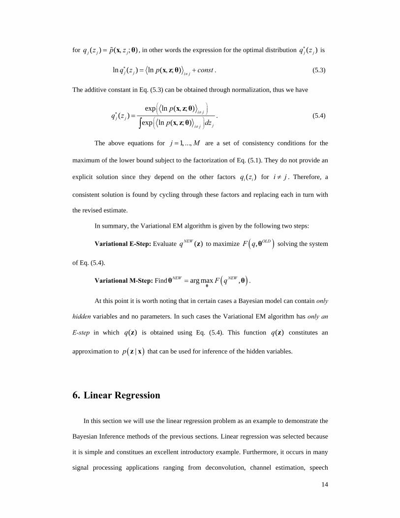
At this point it is worth noting that in certain cases a Bayesian model can contain only

hidden variables and no parameters. In such cases the Variational EM algorithm has only an

E-step in which ( )q z is obtained using Eq. (5.4). This function ( )q z constitutes an

approximation to ( )|p z x that can be used for inference of the hidden variables.

6. Linear Regression

In this section we will use the linear regression problem as an example to demonstrate the

Bayesian Inference methods of the previous sections. Linear regression was selected because

it is simple and constitues an excellent introductory example. Furthermore, it occurs in many

signal processing applications ranging from deconvolution, channel estimation, speech

15

recognition, frequency estimation, time series prediction and system identification.

For this problem, we consider an unknown signal ( )y ∈ℜx , N∈Ω⊆ℜx and want to

predict its value ( )t y∗ ∗= x at an arbitrary location ∗ ∈Ωx , using a vector 1( )TNt … t= , ,t of

N noisy observations ( )n n nt y ε= +x , at locations 1( )TN…= , ,x x x , n ∈Ωx , 1n … N= , , .

The additive noise nε is commonly assumed to be independent, zero-mean, Gaussian

distributed:

1( ) ( 0 )p N β −= | , ,ε ε I (6.1)

where β is the inverse variance and 1( )TN…ε ε= , ,ε .

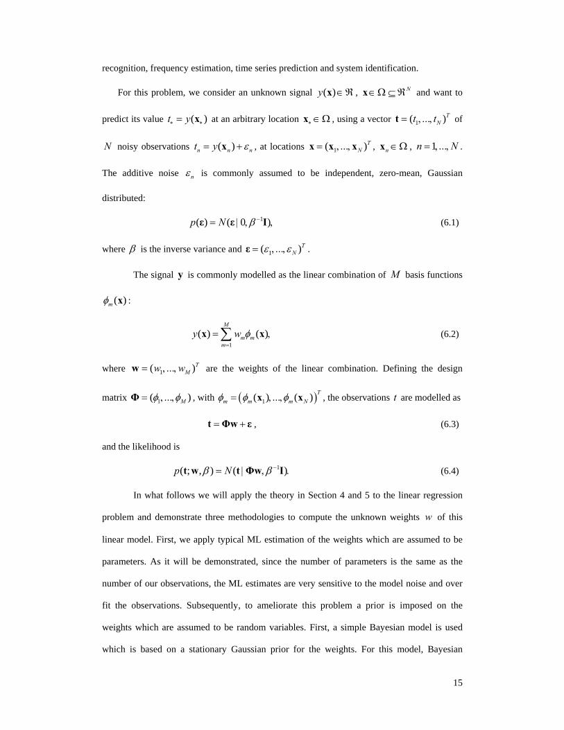
The signal y is commonly modelled as the linear combination of M basis functions

( )mφ x :

1

( ) ( )M

m mm

y w φ=

= ,∑x x (6.2)

where 1( )TMw … w= , ,w are the weights of the linear combination. Defining the design

matrix 1( )M…φ φ= , ,Φ , with ( )1( ) ( ) Tm m m N…φ φ φ= , ,x x , the observations t are modelled as

= +t Φw ε , (6.3)

and the likelihood is

1( ; , ) ( )p Nβ β −= | , .t w t Φw I (6.4)

In what follows we will apply the theory in Section 4 and 5 to the linear regression

problem and demonstrate three methodologies to compute the unknown weights w of this

linear model. First, we apply typical ML estimation of the weights which are assumed to be

parameters. As it will be demonstrated, since the number of parameters is the same as the

number of our observations, the ML estimates are very sensitive to the model noise and over

fit the observations. Subsequently, to ameliorate this problem a prior is imposed on the

weights which are assumed to be random variables. First, a simple Bayesian model is used

which is based on a stationary Gaussian prior for the weights. For this model, Bayesian

16

inference is performed using the EM algorithm and the resulting solution is robust to noise.

Nevertheless, this Bayesian model is very simplistic and does not have the ability to capture

the local signal properties. For this purpose it is possible to introduce a more sophisticated

spatially varying hierarchical model which is based on a non-stationary Gaussian prior for the

weights and a hyperprior. This model is too complex to solve using the EM algorithm. For

this purpose, the variational Bayesian methodology described in Section 5 is used to infer

values for the unknowns of this model. Finally, the three methods are used to obtain

estimates of a simple artificial signal, in order to demonstare that the added complexity in the

Bayesian model improves the solution quality. In Figure 3(a), (b) and (c) we show the

graphical models for the three approaches to Linear Regression.

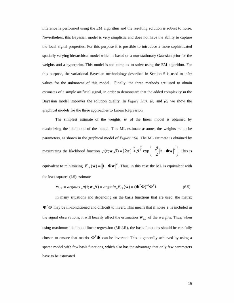
The simplest estimate of the weights w of the linear model is obtained by

maximizing the likelihood of the model. This ML estimate assumes the weights w to be

parameters, as shown in the graphical model of Figure 3(a). The ML estimate is obtained by

maximizing the likelihood function ( ) 222( ; , ) 2 exp2

NN

p ββ π β− ⎛ ⎞= − −⎜ ⎟⎝ ⎠

t w t Φw . This is

equivalent to minimizing 2( )LSE = −w t Φw . Thus, in this case the ML is equivalent with

the least squares (LS) estimate

1( ; , ) ( ) ( )T TLS LSw wp Eargmax argminβ −= = = .w t w w Φ Φ Φ t (6.5)

In many situations and depending on the basis functions that are used, the matrix

TΦ Φ may be ill-conditioned and difficult to invert. This means that if noise ε is included in

the signal observations, it will heavily affect the estimation LSw of the weights. Thus, when

using maximum likelihood linear regression (MLLR), the basis functions should be carefully

chosen to ensure that matrix TΦ Φ can be inverted. This is generally achieved by using a

sparse model with few basis functions, which also has the advantage that only few parameters

have to be estimated.

17

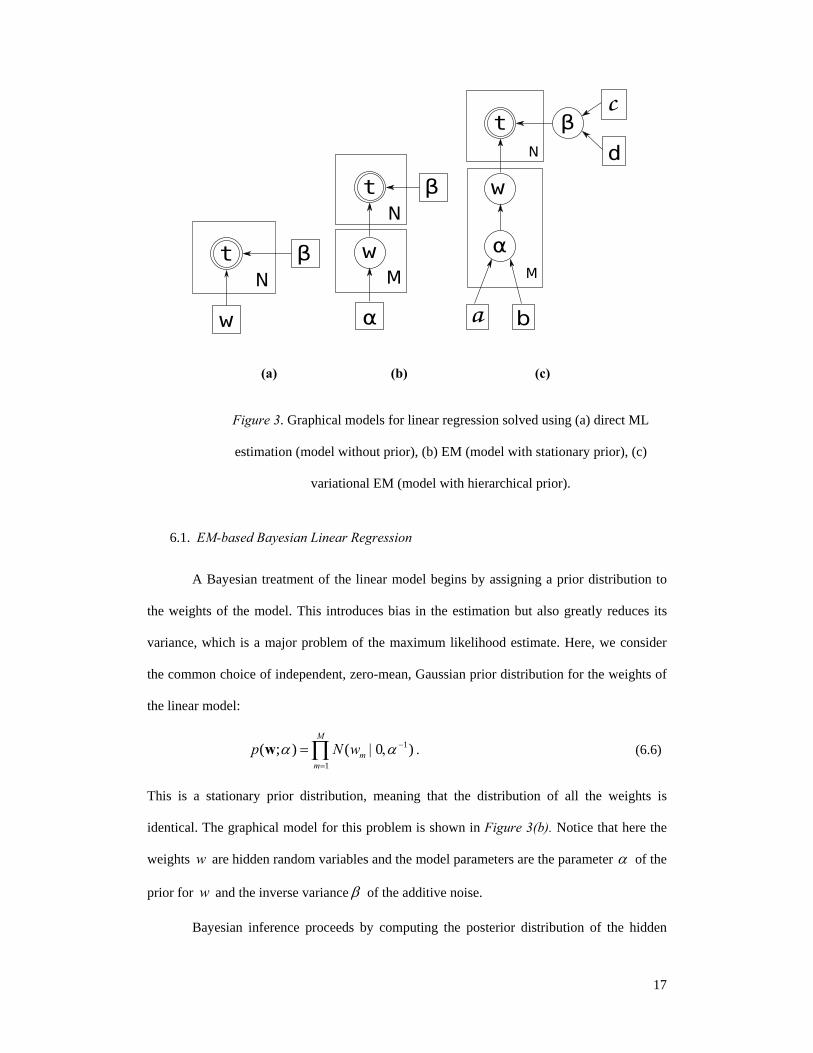
(a) (b) (c)

Figure 3. Graphical models for linear regression solved using (a) direct ML

estimation (model without prior), (b) EM (model with stationary prior), (c)

variational EM (model with hierarchical prior).

6.1. EM-based Bayesian Linear Regression

A Bayesian treatment of the linear model begins by assigning a prior distribution to

the weights of the model. This introduces bias in the estimation but also greatly reduces its

variance, which is a major problem of the maximum likelihood estimate. Here, we consider

the common choice of independent, zero-mean, Gaussian prior distribution for the weights of

the linear model:

1

1

( ; ) ( 0 )M

mm

p N wα α −

=

= | ,∏w . (6.6)

This is a stationary prior distribution, meaning that the distribution of all the weights is

identical. The graphical model for this problem is shown in Figure 3(b). Notice that here the

weights w are hidden random variables and the model parameters are the parameter α of the

prior for w and the inverse variance β of the additive noise.

Bayesian inference proceeds by computing the posterior distribution of the hidden

18

variables:

( ) ( )( )

( )p pp

pβ αα βα β

| ; ;| ; , = .

; ,t w ww t

t (6.7)

Notice, that the marginal likelihood ( )p α β; ,t that appears on the denominator can be

computed analytically:

1 1( ) ( ) ( ) ( 0 )Tp p p d Nα β β α β α− −; , = | ; ; = | , + .∫t t w w w t I ΦΦ (6.8)

Then, the posterior of the hidden variables is:

( ) ( )p Nα β| ; , = | , ,w t w μ Σ (6.9)

with

Tβ= ,μ ΣΦ t (6.10)

1( )Tβ α −= + .Σ Φ Φ I (6.11)

The parameters of the model can be estimated by maximizing the logarithm of the marginal

likelihood ( )p α β; ,t which yields

( ){ }11 1 1 1

,( , ) argmin log T T T

ML MLα β

α β β α β α−− − − −= + + +I ΦΦ t I ΦΦ t . (6.12)

Direct optimization of (6.12) presents several computational difficulties, since its

derivatives with respect to the parameters ( ),α β are difficult to compute. Furthermore, the

problem requires a constrained optimization algorithm since the estimates of ( ),α β have to

be positive since they represent inverse variances. Instead, the EM algorithm described in

Section 4, provides an efficient framework to simultaneously obtain estimates for ( ),α β and

infer values for w . Notice, that although the EM algorithm does not involve computations

with the marginal likelihood (6.8), the algorithm converges to a local maximum of it. After

initializing the parameters to some values ( )(0) (0),α β , the algorithm proceeds by iteratively

performing the following steps:

19

• E- step

Compute the expected value of the logarithm of the complete likelihood :

( ) ( )

( ) ( )

( )

( )

( )

( ) ln ( )

ln ( ) ( ) .

t t

t t

t

p

p

Q p

p pα β

α β

α β α β

α β α β| ; ,

| ; ,

, ; , = , ; , =

| ; , ; ,w t

w t

t w t w

t w w (6.13)

This is computed using equations (6.4) and (6.6) as

( ) ( )

( )

2 2( )

2 2

( ) ln ln const2 2 2 2

ln ln const.2 2 2 2

t N MQ

N M

β αα β β α

β αβ α

, ; , = − − + − +

= − − + − +

t w t Φw w

t Φw w(6.14)

These expected values are with respect to ( ) ( )( )t tp α β| ; ,w t and can be computed from (6.9), giving

( )( )

2( ) ( ) ( )

2( ) ( )

( ) ln [ ]2 2

ln [ ] const, 2 2

t t T t

t t

NQ tr

M tr

βα β β

αα

, ; , = − − + +

− + +

t w t Φμ Φ Σ Φ

μ Σ (6.15)

where ( )tμ and ( )tΣ are computed using the current estimates of the parameters ( )tα and

( )tβ :

( ) ( ) ( )t t t Tβ= ,μ Σ Φ t (6.16)

( ) ( ) ( ) 1( )t t T tβ α −= + .Σ Φ Φ I (6.17)

• M-step

Maximize ( ) ( )tQ α β, ; ,t w with respect to the parameters α and β :

( 1) ( 1) ( )( )( ) ( )t t tQargmax α βα β α β+ +

,, = , ; ,t w . (6.18)

The derivatives of ( ) ( )tQ α β, ; ,t w with respect to the parameters are:

( )( ) 2( ) ( )( ) 1 [ ]

2 2

tt tQ M trα β

α α∂ , ; ,

= − + ,∂t w μ Σ (6.19)

( )( ) 2( ) ( )( ) 1 [ ]

2 2

tt T tQ N trα β

β β∂ , ; ,

= − − +∂t w t Φμ Φ Σ Φ . (6.20)

Setting these to zero, we obtain the following formulas to update the parameters α and β :

20

( 1)2( ) ( )[ ]

t

t t

M

trα + = ,

+μ Σ (6.21)

( 1)2( ) ( )[ ]

t

t T t

N

trβ + = .

− +t Φμ Φ Σ Φ (6.22)

Notice, that the maximization step can be analytically performed, in contrast to direct

maximization of the marginal likelihood in (6.8), which would require numerical

optimization. Furthermore, equations (6.21) and (6.22) guarantee that positive estimations for

the parameters α and β are produced, which is a requirement since these represent inverse

variance parameters. However, the parameters should be initialized with care, since

depending on the initialization a different local maximum may be attained. Inference for w is

obtained directly since the sufficient statistics of the posterior ( )p α β| ; ,w t are computed in

the E-step. The mean of this posterior (Eq (6.16)) can be used as Bayesian linear minimum

mean square error (LMMSE) inference for w .

6.2. Variational EM-Based Bayesian Linear Regression

In the Bayesian approach described in the previous section, due to the use of a

stationary Gaussian prior distribution for the weights of the linear model, exact computation

of the marginal likelihood is possible and Bayesian inference is performed analytically.

However, in many situations, it is important to allow the flexibility to model local

characteristics of the signal, which the simple stationary Gaussian prior distribution is unable

to do. For this reason, a non-stationary Gaussian prior distribution with a distinct inverse

variance mα for each weight is considered:

1

1

( ) ( 0 )M

m mm

p N w α−

=

| = | ,∏w α . (6.23)

However, such a model is over-parameterized since there are almost as many observations as

parameters to be estimated. For this purpose the precision parameters 1( )TMα α= , ,α … are

constrained, by treating them as random variables and imposing a Gamma prior distribution

21

to them according to

1

( ) ( )M

mm

p a b Gamma a bα=

; , = | ,∏α . (6.24)

This prior is selected because it is “conjugate” to the Gaussian [13]. Furthermore, we assume

a Gamma distribution as prior for the noise inverse variance β :

( ) ( )p c d Gamma c dβ β; , = | , . (6.25)

The graphical model for this Bayesian approach is shown in Figure 3(c) where the

dependence of the hidden variables w on the hidden variables α is apparent. Also the

parameters , ,a b c and d of this model and the hidden variables that depend on them are also

apparent.

Bayesian inference requires the computation of the posterior distribution

( | , ) ( | ) ( ) ( )( , , | )

( )p p p pp

pβ ββ =

t w w α αw α tt

. (6.26)

However, the marginal likelihood ( ) ( | , ) ( | ) ( ) ( )p p p p p d d dβ β β= ∫t t w w α α w α cannot

be computed analytically, and thus the normalization constant in Eq. (6.26) cannot be

computed. Thus, we resort to approximate Bayesian inference methods and specifically to the

variational inference methodology. Assuming posterior independence between the weights w

and the variance parameters α and β ,

( ) ( ) ( ) ( ) ( )p a b c d q q q qβ β β, , | ; , , , ≈ , , = ,w α t w α w α (6.27)

the approximate posterior distributions q can be computed from (5.3) as follows. Keeping

only the terms of ln ( )q w that depend on w , we have:

22

( )

( ) ( )

( ) ( )

( ) ( )

2

1 ( ) ( )

2

1

ln ( ) ln ( ) const

ln ( ) ( ) const

ln ( ) ln ( ) const

1( ) ( ) const2 2

1[ 2 ] const2 2

12

q q

q q

q q

MT

m mm q q

MT T T T

m mm

TT T

q p

p t p

p t p

w

w

β

β

β

β

β

β

β

β α

β α

β β

=

=

= , , , +

= | , | +

= | , + | +

= − − − − +

=− − + − +

=− + −

∑

∑

α

α

α

α

w t w α

w w α

w w α

t Φw t Φw

t t t Φw w Φ Φw

w Φ Φ A w w

1 1

const

1 const,2

T

T T− −

+

= − − +

Φ t

w Σ w w Σ μ

(6.28)

where 1 Mdiag( ,..., )α α=A .

Notice, that this is the exponent of a Gaussian distribution with mean μ and

covariance matrix Σ given by

Tβ= ,μ ΣΦ t (6.29)

( ) 1Tβ−

= + .Σ Φ Φ A (6.30)

Therefore, ( )q w is given by:

( ) ( )q N= | , .w w μ Σ (6.31)

The posterior ( )q α is similarly obtained by computing the terms of ln ( )q α that

depend on α :

( ) ( )

( )

2

1 1 1 1

2

1 1

1 1

ln ( ) ln ( )

ln ( ) ( )

1 ln ( 1) ln2

1 1ln2 2

ln ,

q q

q

M M M M

m m m m mm m m m

M M

mmm m

M M

m mmm m

q p

p p

w a b

a w b

a constb

ββ

α α α α

α

α α

= = = =

= =

= =

= , , ,

= |

= − + − −

⎛ ⎞ ⎛ ⎞= − − +⎜ ⎟ ⎜ ⎟⎝ ⎠ ⎝ ⎠

= − +

∑ ∑ ∑ ∑

∑ ∑

∑ ∑

w

w

α t w α

w α α

(6.32)

This is the exponent of the product of M independent Gamma distributions with

parameters a and mb , given by

23

1 2a a= + / , (6.33)

212m mb b w= + . (6.34)

Thus, ( )q α is given by:

1

( ) ( )M

m mm

q Gamma a bα=

= | , .∏α (6.35)

The posterior distribution of the noise inverse variance can be similarly computed as:

( ) ( )q Gamma c dβ β= | , , (6.36)

with

2c c N= + / , (6.37)

21

2d d= + − .t Φw (6.38)

The approximate posterior distributions in equations (6.31), (6.35) and (6.36) are then

iteratively updated until convergence, since they depend on the statistics of each other, see for

details [29].

Notice here, that the ‘true’ prior distribution of the weights can be computed by

marginalizing the hyper-parameters α

1

1

1

( ) ( ) ( )

( 0 ) ( )

( ).

M

m m m mm

m

mm

p b p p a b d

N w Gamma a b d

St w

α α α

λ ν

−

=

=

; , = | ; ,

= | , | ,

= | ,

∫

∏∫

∏

w a w α α α

(6.39)

and is a Student-t pdf, ( 1)/21/2 2(( 1) / 2) ( )( | , , ) 1

( / 2)xSt x

νν λ λ μμ λ νν πν ν

− +⎡ ⎤Γ + −⎛ ⎞= +⎜ ⎟ ⎢ ⎥Γ ⎝ ⎠ ⎣ ⎦

, with

mean 0μ = , parameter /a bλ = and degrees of freedom 2aν = . This distribution, for

small degrees of freedom ν , exhibits very heavy tails. Thus, it favours sparse solutions,

24

which include only few of the basis functions and prunes the remaining basis functions by

setting the corresponding weights to very small values. Those basis functions that are actually

used in the final model are called relevance basis functions.

Notice, that for simplicity we have assumed fixed the parameters a , b , c and d of the

Student-t distributions. In practice we can often obtain good results by assuming

uninformative distributions, which are obtained by setting these parameters to very small

values, i.e. 610a b c d −= = = = . Alternatively, we can estimate these parameters using a

Variational EM algorithm. Such an algorithm would add an M-step to the described method,

in which the Variational bound would be maximized with respect to these parameters.

However, the typical approach in Bayesian modeling is to fix the hyperparameters to define

uninformative hyperpriors at the highest level of the model.

6.3. Linear Regression Examples

Next, we present numerical examples to demonstrate the properties of the previously

described linear regression models. We also demonstrate the advantages that can be reaped by

using the variational Bayesian inference. An artificially generated signal ( )y x is used so that

the “ground truth” is known. We have obtained 50N = samples of the signal and added

Gaussian noise of variance 2 24 10σ −= × , which corresponds to signal to noise ratio

6.6SNR dB= . We used N basis functions and, specifically, one basis function centred at

the location of each signal observation. The basis functions were Gaussian kernels of the form

2

212

( ) ( ) exp( )i i iKφσ

φ = , = − −x x x x x . (6.40)

In this example we set 0a b= = , in order to obtain a very heavy-tailed, uninformative

Student-t distribution.

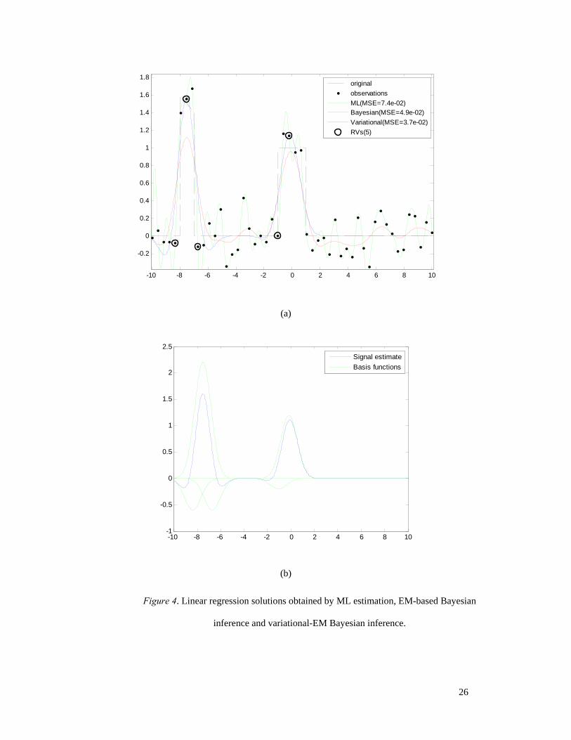
We then used the observations to predict the output of the signal, using i) ML

estimation, Eq. (6.5) ii) EM-based Bayesian inference, Eq. (6.16) and iii) variational EM-

based Bayesian inference, Eq. (6.29). Results are shown in Fig. 4(a). Notice, that the ML

estimate follows exactly the noisy observations. Thus, it is the worst in terms of mean square

25

error. This should be expected, since in this formulation we use as many basis functions as the

observations and there is no constraint on the weights. The Bayesian methodology overcomes

this problem since the weights are constrained by the priors. However, since this signal

contains regions with large variance and some with very small variance, it is clear that the

stationary prior is not capable of accurately modelling its local behaviour. In contrast, the

hierarchical non-stationary prior is more flexible and seems to achieve better local fit.

Actually, the solution corresponding to the latter prior, uses only a small subset of the basis

functions, whose locations are shown as circled observations in Fig. 4(a). This happens

because we have set 0a b= = , which defines an uninformative Student-t distribution.

Therefore, most weights are estimated to be exactly zero and only few basis functions are

used in the signal estimation. Those basis functions that are actually used in the final model

are called relevance basis function and the vectors where they are centered are called

relevance vectors and denoted as (RV) in Fig. 4(a). The relevance basis functions are plotted

in Fig. 4(b) in order to demonstrate how the signal estimation is obtained by addition of these

basis functions.

26

-10 -8 -6 -4 -2 0 2 4 6 8 10

-0.2

0

0.2

0.4

0.6

0.8

1

1.2

1.4

1.6

1.8

originalobservationsML(MSE=7.4e-02)Bayesian(MSE=4.9e-02)Variational(MSE=3.7e-02)RVs(5)

(a)

-10 -8 -6 -4 -2 0 2 4 6 8 10-1

-0.5

0

0.5

1

1.5

2

2.5

Signal estimateBasis functions

(b)

Figure 4. Linear regression solutions obtained by ML estimation, EM-based Bayesian

inference and variational-EM Bayesian inference.

27

7. Gaussian Mixture Models

Gaussian mixture models (GMM) are a valuable statistical tool for modelling

densities. They are flexible enough to approximate any given density with high accuracy and

in addition, they can be interpreted as a soft clustering solution. They have been widely used

in a variety of signal processing problems ranging from speech understanding, image

modelling, tracking, segmentation, recognition, watermarking, and denoising.

A GMM is defined as a convex combination of Gaussian densities and is widely used

to describe the density of a dataset in cases where a single distribution does not suffice. To

define a mixture model with M components we have to specify the probability density

( )jp x of each component j as well as the probability vector 1( )M…π π, , containing the

mixing weights jπ of the components ( 0jπ ≥ and 1

1Mjj

π=

=∑ ).

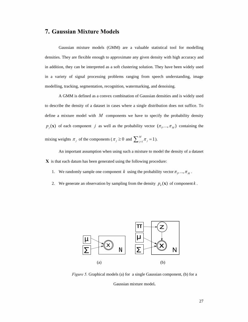
An important assumption when using such a mixture to model the density of a dataset

X is that each datum has been generated using the following procedure:

1. We randomly sample one component k using the probability vector 1 M…π π, , .

2. We generate an observation by sampling from the density ( )kp x of component k .

(a) (b)

Figure 5. Graphical models (a) for a single Gaussian component, (b) for a

Gaussian mixture model.

28

The graphical model corresponding to above generation process is presented in Figure 5 (b),

where the discrete hidden random variable Z represents the component that has been

selected to generate an observed sample x , i.e. to assign the value =X x to the observed

random variable X . In this graphical model the node distributions are ( ) jP Z j π= = and

( ) ( )jP Z j p= | = =X x x . For the joint pdf of X and Z it holds that

( ) ( ) ( )p Z p Z p Z, = |X X , (7.1)

and through marginalization of Z we obtain the well-known formula for mixture models:

1 1

( ) ( ) ( ) ( )M M

j jj j

p p Z j p Z j pπ= =

= = = | = = =∑ ∑X x X x x . (7.2)

In the case of GMMs, the density of each component j is ( ) ( )j j jp N= ; ,x x μ Σ

where dj ∈ℜμ denotes the mean and jΣ is the d d× covariance matrix. Therefore

1

( ) ( )M

j j jj

p Nπ=

= ; ,∑x x μ Σ . (7.3)

A notable convenience in mixture models is that using Bayes’ theorem it is

straightforward to compute the posterior probability ( ) ( )P j p Z j| = = |x x that an

observation x has been generated by sampling from the distribution of mixture component j :

1

( )( ) ( )( )( ) ( )

j j jM

l l ll

Np Z j p Z jP jp N

π

π=

| ,| = =| = =

| ,∑x μ Σxx

x x μ Σ. (7.4)

This probability is sometimes referred to as the responsibility of component j for generating

observation x . In addition, by assigning a data point x to the component with maximum

posterior, it is easy to obtain a clustering of the dataset X into M clusters, with one cluster

corresponding to each mixture component.

7.1. EM for GMM training

Let { }1dn n n … N= | ∈ℜ , = , ,X x x denote a set of data points to be modelled using

29

a GMM with M components: 1

( ) ( )Mj n j jj

p Nπ=

= | ,∑x x μ Σ . We assume that the number

of components M is specified in advance. The vector θ of mixture parameters to be

estimated consists of the mixing weights and the parameters of each component, i.e.

{ }1j j j j … Mπ= , , | = , ,θ μ Σ .

Parameter estimation can be achieved through the maximization of the log-likelihood:

log ( )ML argmax p= ;θθ X θ , (7.5)

where assuming independent and identically distributed observations the likelihood can be

written as

11 1

( ) ( ) ( )N N M

n j n j jjn n

p p Nπ== =

; = ; = ; ,∑∏ ∏X θ x θ x μ Σ . (7.6)

From the graphical model in Fig. 5(b) it is clear that to each observed variable

n ∈x X corresponds a hidden variable nz representing the component that was used to

generate nx . This hidden variable can be represented using a binary vector with M elements

jnz , such that 1jnz = if nx has been generated from mixture component j and 0jnz =

otherwise. Since 1jnz = with probability jπ and 1

1Mjj

π=

=∑ , then nz follows the

multinomial distribution. Let { }1n n … N= , = , ,Z z denote the set of hidden variables. Then

( )p |Z θ is written

1 1

( ) jnN M

zj

n j

p π= =

; =∏∏Z θ , (7.7)

and

1 1

( | ; ) ( ) jnN M

zn j j

n j

p N= =

= ; ,∏∏X Z θ x μ Σ . (7.8)

As previously noted, the convenient issue with mixture models is that we can easily compute

the exact posterior ( 1 )jn np z = | ;x θ of the hidden variables given the observations using Eq.

(7.4). Therefore application of the exact EM algorithm is feasible.

30

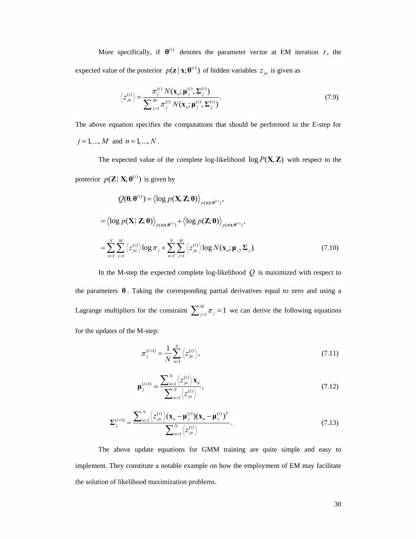
More specifically, if ( )tθ denotes the parameter vector at EM iteration t , the

expected value of the posterior ( )( | ; )tp z x θ of hidden variables jnz is given as

( ) ( ) ( )

( )( ) ( ) ( )

1

( )

( )

t t tj n j jt

jn M t t tj n j jj

Nz

N

π

π=

; ,=

; ,∑x μ Σ

x μ Σ. (7.9)

The above equation specifies the computations that should be performed in the E-step for

1j … M= , , and 1n … N= , , .

The expected value of the complete log-likelihood log ( )P ,X Z with respect to the

posterior ( )( )tp | ;Z X θ is given by

( )( )

( | ; )( ) log ( ) t

tp

Q p, = , ;z x θ

θ θ X Z θ ,

( ) ( )( | ; ) ( | ; )log ( ) log ( )t tp p

p p= | ; + ;z x θ z x θ

X Z θ Z θ ,

( ) ( )

1 1 1 1log log ( )

N M N Mt t

jn j jn n j jn j n j

z z Nπ= = = =

= + ; , .∑∑ ∑∑ x μ Σ (7.10)

In the M-step the expected complete log-likelihood Q is maximized with respect to

the parameters θ . Taking the corresponding partial derivatives equal to zero and using a

Lagrange multipliers for the constraint 1

1Mjj

π=

=∑ we can derive the following equations

for the updates of the M-step:

( 1) ( )

1

1 ,N

t tj jn

nz

Nπ +

=

= ∑ (7.11)

( )

( 1) 1( )

1

,N t

jn nt nj N t

jnn

z

z+ =

=

= ∑∑

xμ (7.12)

( ) ( ) ( )

( 1) 1( )

1

( )( )N t t t Tjn n j n jt n

j N tjnn

z

z+ =

=

− −= ∑

∑x μ x μ

Σ . (7.13)

The above update equations for GMM training are quite simple and easy to

implement. They constitute a notable example on how the employment of EM may facilitate

the solution of likelihood maximization problems.

31

−6 −4 −2 0 2 4 6

−6

−4

−2

0

2

4

6

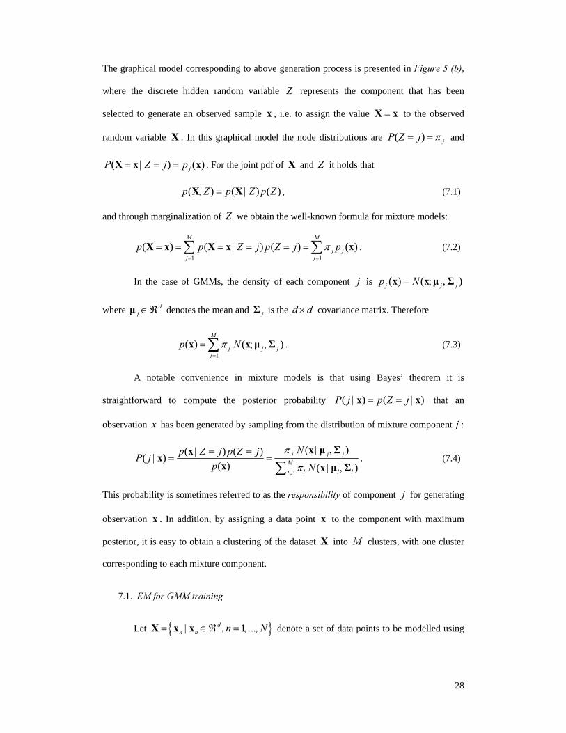
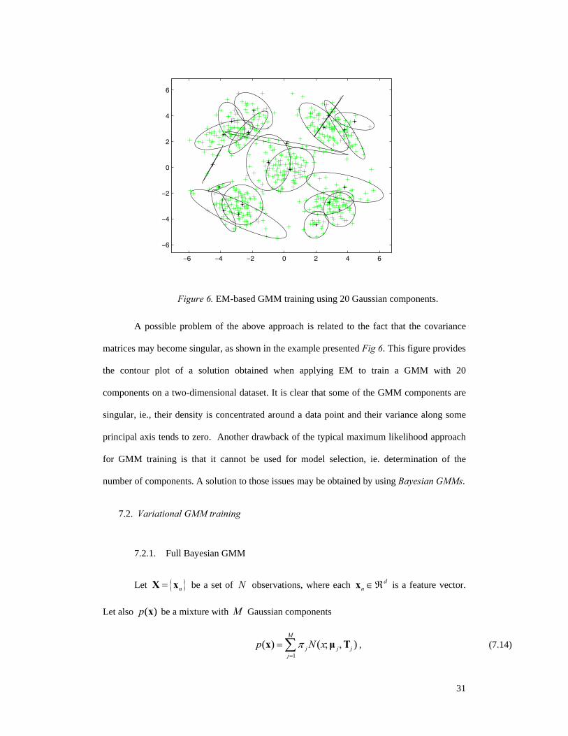
Figure 6. EM-based GMM training using 20 Gaussian components.

A possible problem of the above approach is related to the fact that the covariance

matrices may become singular, as shown in the example presented Fig 6. This figure provides

the contour plot of a solution obtained when applying EM to train a GMM with 20

components on a two-dimensional dataset. It is clear that some of the GMM components are

singular, ie., their density is concentrated around a data point and their variance along some

principal axis tends to zero. Another drawback of the typical maximum likelihood approach

for GMM training is that it cannot be used for model selection, ie. determination of the

number of components. A solution to those issues may be obtained by using Bayesian GMMs.

7.2. Variational GMM training

7.2.1. Full Bayesian GMM

Let { }n=X x be a set of N observations, where each dn ∈ℜx is a feature vector.

Let also ( )p x be a mixture with M Gaussian components

1

( ) ( )M

j j jj

p N xπ=

= ; ,∑x μ T , (7.14)

32

where jπ⎧ ⎫⎨ ⎬⎩ ⎭

=π are the mixing coefficients (weights), j⎧ ⎫⎨ ⎬⎩ ⎭

=μ μ the means (centers) of the

components, and j⎧ ⎫⎨ ⎬⎩ ⎭

=T T the precision (inverse covariance) matrices (it must be noted that

in Bayesian GMMs it is more convenient to use the precision matrix instead of the covariance

matrix).

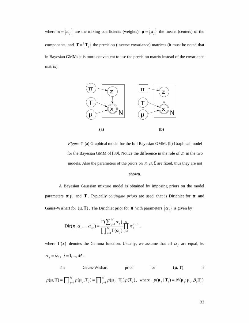
(a) (b)

Figure 7. (a) Graphical model for the full Bayesian GMM. (b) Graphical model

for the Bayesian GMM of [30]. Notice the difference in the role of π in the two

models. Also the parameters of the priors on , ,π μ Σ are fixed, thus they are not

shown.

A Bayesian Gaussian mixture model is obtained by imposing priors on the model

parameters ,π μ and T . Typically conjugate priors are used, that is Dirichlet for π and

Gauss-Wishart for ( ),μ T . The Dirichlet prior for π with parameters jα⎧ ⎫⎨ ⎬⎩ ⎭

is given by

111

11

( )Dir( )

( )j

MMjj

M jMjjj

… ααα α π

α−=

==

Γ| , , =

Γ

∑∏

∏π ,

where ( )xΓ denotes the Gamma function. Usually, we assume that all jα are equal, ie.

0jα α= , 1j … M= , , .

The Gauss-Wishart prior for ( ),μ T is

1 1( ) ( ) ( ) ( )M M

j j j j jj jp p p p

= =, = , = |∏ ∏μ T μ T μ T T , where 0 0( ) ( )j j j jp N β| = ; ,μ T μ μ T

33

(with parameters 0μ and 0β ) and ( )jp T is the Wishart distribution

( 1) 2 12

2 ( 1) 4 21

expW( )

2 (( 1 ) 2)

dj j

j dd d d ni

tr

i

ν

νν

π ν

− − / ⎧ ⎫⎨ ⎬⎩ ⎭

/ − / − /=

| | −| , =

| | Γ + − /∏T VT

T VV

,

with parameters ν and V denoting the degrees of freedom and the scale matrix respectively.

Notice, that the Wishart distribution, is the multidimensional generalization of the Gamma

distribution. In linear regression we used the Gauss – Gamma prior, assuming independent

precisions iα and thus assigning them independent Gamma prior distributions. Here,

however, because there may be significant correlations between data, we could use the

Wishart prior to capture these correlations.

The graphical model corresponding to this Bayesian GMM is presented in Fig. 7(a).

This is a full Bayesian GMM and if all the hyperparameters (ie. the parameters 0 0α μ β ν, , ,

and V of the priors) are specified in advance, then the model does not contain any parameter

to be estimated, but only hidden random variables ( )h = , , ,Z π μ T whose posterior ( )p |h X

given the data must be computed. It is obvious that in this case the posterior cannot be

computed analytically, thus an approximation ( )q h is computed by applying the variational

mean-field equations (5.3) to the specific Bayesian model [30].

The mean-field approximation assumes q to be a product of the form

( ) ( ) ( ) ( , )Z Tq q q qπ μ= .h Z π μ T (7.15)

and the solution is given by eq. (5.3). After performing the necessary calculations, the result is

the following set of densities:

1 1

( ) jnN M

zZ jn

n j

q r= =

=∏∏Z , (7.16)

( ) ( { })jq Dirπ λ= |π π , (7.17)

1

( ) ( ) ( )M

T j j T jj

q q qμ μ=

, = |∏μ T μ T T , (7.18)

34

1

( ) ( )M

j j j j jj

q Nμ β=

| = ; ,∏μ T μ m T , (7.19)

1

( ) ( )M

T j j jj

q W η=

= ; ,∏T T U . (7.20)

and the detailed formulas for updating the parameters ( jn j j j j jr λ β η, , , , ,m U ) of the densities

can be found in [30]. By solving the above system of equations using a simple iterative update

procedure we obtain an optimal approximation ( )q h to the true posterior ( )p |h X under the

mean-field constraint.

The typical approach in Bayesian modelling is to specify the hyperparameters α , ν ,

V , 0μ , 0β of the model so that uninformative prior distributions are defined. We follow this

approach, although it would be possible to incorporate an M-step to the algorithm, in order to

adjust these parameters. However, this is usually not followed.

An advantage of the full Bayesian GMM compared to GMM without priors is that it

does not allow the singular solutions often arising in the maximum likelihood approach where

a Gaussian component becomes responsible for a single data point. A second advantage is

that it is possible to use the Bayesian GMM for directly determining the optimal number of

components without resorting to methods such as cross-validation. However, the

effectiveness of the full Bayesian mixture is limited for this problem, since the Dirichlet prior

does not allow mixing weight of a component to become zero and to be eliminated from the

mixture. Also in this case the final result depends highly on the hyperparameters of the priors

(and especially of the parameters of the Dirichlet prior) that must be specified in advance

[13]. For a specific set of hyperparameters, it is possible to run the variational algorithm for

several values of the number M of mixture components and keep the solution corresponding

to the best value of the variational lower bound.

7.2.2. Removing the prior from the mixing weights

In [22] another example of a Bayesian GMM model has been proposed that does not

35

assume a prior on the mixing weights jπ⎧ ⎫⎨ ⎬⎩ ⎭

, which are treated as parameters and not as

random variables. The graphical model for this approach is depicted in Fig. 7(b).

In this Bayesian GMM, which we will call CB model from the initials of the two

authors of this work, Gaussian and Wishart priors are assumed for μ and T respectively

1

( ) ( 0 )M

jj

p N β=

= | ,∏μ μ I , (7.21)

1

( ) ( )M

jj

p W ν=

= | , .∏T T V (7.22)

This Bayesian model is capable (to some extent) to estimate the optimal number of

components. This is achieved through maximization of the marginal likelihood ( )p ;X π

obtained by integrating out the hidden variables { }= , ,h Z μ T

( ) ( )p p d; = , ;∫X π X h π h , (7.23)

with respect to the mixing weights π that are treated as parameters. The variational

approximation suggests the maximization of a lower bound of the logarithmic marginal

likelihood

( )[ ] ( ) log log ( )( )

pF q q d pq, ;

, = ≤ ;∫X h ππ h h X π

h, (7.24)

where ( )q h is an arbitrary distribution approximating the posterior ( )p |h X . A notable

property is that during maximization of F , if some of the components fall in the same region

in the data space, then there is strong tendency in the model to eliminate the redundant

components (ie. setting their jπ equal to zero), once the data in this region are sufficiently

explained by fewer components. Consequently, the competition between mixture components

suggests a natural approach for addressing the model selection problem: fit a mixture

initialized with a large number of components, and let competition eliminate the redundant.

Following the variational methodology our aim is to maximize the lower bound F of

the logarithmic marginal likelihood log ( )p ;X π :

36

( )[ ] ( ) log( )

pF q q d dq, , , ;

, = , ,, ,∑ ∫

Z

X Z μ T ππ Z μ T μ TZ μ T

, (7.25)

where q is an arbitrary distribution that approximates the posterior distribution

( )p , , | ;Z μ T X π . The maximization of F is performed in an iterative way using the

Variational EM algorithm. At each iteration two steps take place: first maximization of the

bound with respect to q and, subsequently, maximization of the bound with respect to π .

To implement the maximization with respect to q the mean-field approximation has

been adopted (eq. (5.1)) that assumes q to be a product of the form

( ) ( ) ( ) ( )Z Tq q q qμ=h Z μ T . (7.26)

After performing the necessary calculations in eq.(5.3), the result is the following set of

densities:

1 1

( ) jnN M

zZ jn

n j

q r= =

=∏∏Z , (7.27)

1

( ) ( )M

j j jj

q Nμ=

= | ,∏μ μ m S , (7.28)

1

( ) ( )M

T j j jj

q W η=

= | ,∏T T U , (7.29)

where the parameters of the densities can be computed as:

1

jnjn M

knk

rrr=

=∑

, (7.30)

{1 1exp log

2 2TT T T

jn j j j n n n j j n j jtrr π⎫⎧ ⎫⎛ ⎞⎪ ⎪⎪⎜ ⎟⎨ ⎬⎬⎜ ⎟⎪ ⎪⎪⎝ ⎠⎩ ⎭⎭

= | | − − + +T T x x x μ μ x μ μ ,(7.31)

1

1

N

j j j jn nn

z−

=

= ∑m S T x , (7.32)

1

N

j j jnn

zβ=

= + ∑S I T , (7.33)

1

,N

j jnn

zη ν=

= +∑ (7.34)

37

1

N TT T Tj jn n n n j j n j j

n

z⎛ ⎞⎜ ⎟⎜ ⎟⎝ ⎠=

= + − − +∑U V x x x μ μ x μ μ . (7.35)

The expectations with respect to ( )q h used in the above equations satisfy the

equations: 1j j jη −=T U ,

1log (0 5( 1 )) ln 2 lnd

j j jii dψ η

=| | = . + − + − | |∑T U , where ψ

denotes the digamma function, defined as '( )ln ( )( )

d xxdx x

ΓΓ =

Γ, j j=μ m ,

1T Tj j j j j

−= +μ μ S m m and jn jnz r= . It can be observed that the densities are coupled

through their expectations, thus an iterative estimation of the parameters is needed. However

in practice a single pass seems to be sufficient for the variational E-step.

After the maximization of F with respect to q , the second step of each iteration of

the training method requires maximization of F with respect to π , leading to the following

simple update equation for the variational M-step:

1

1 1

Njnn

j M Nknk n

r

rπ =

= =

= .∑∑ ∑ (7.36)

The above Variational EM update equations are applied iteratively and converge to a local

maximum of the variational bound. During the optimization some of the mixing coefficients

converge to zero thus the corresponding components are eliminated from the mixture. In this

way complexity control is achieved. This happens because the prior distribution on μ and T

penalizes overlapping components. Qualitatively speaking, the variational bound can be

written as a sum of two terms: the first one is a likelihood term (that depends on the quality of

data fitting) and the other is a penalty term due to the priors that penalizes complex models.

38

−2.5 −2 −1.5 −1 −0.5 0 0.5 1 1.5 2

−2

−1.5

−1

−0.5

0

0.5

1

1.5

2

(a)

−2.5 −2 −1.5 −1 −0.5 0 0.5 1 1.5 2

−2

−1.5

−1

−0.5

0

0.5

1

1.5

2

(b)

−2.5 −2 −1.5 −1 −0.5 0 0.5 1 1.5 2

−2

−1.5

−1

−0.5

0

0.5

1

1.5

2

(c)

−2.5 −2 −1.5 −1 −0.5 0 0.5 1 1.5 2

−2

−1.5

−1

−0.5

0

0.5

1

1.5

2

(d)

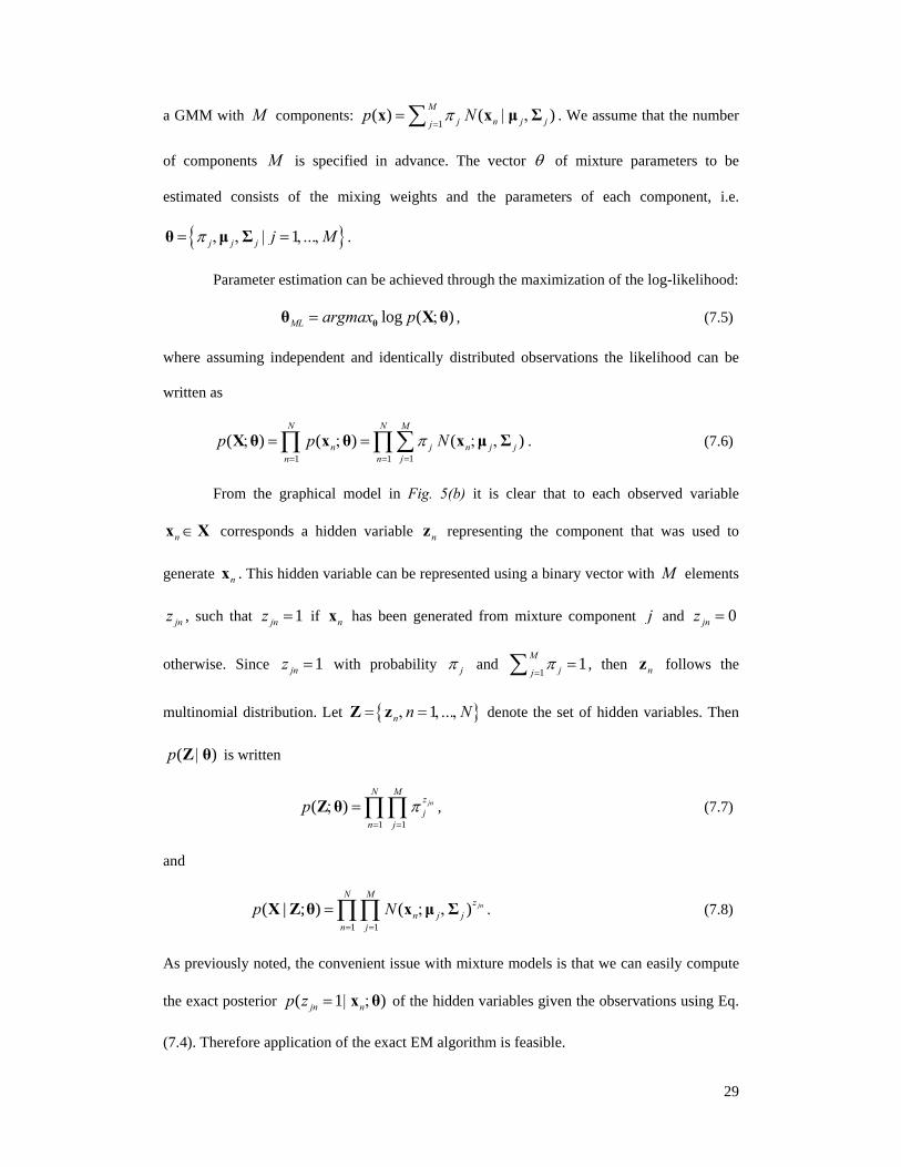
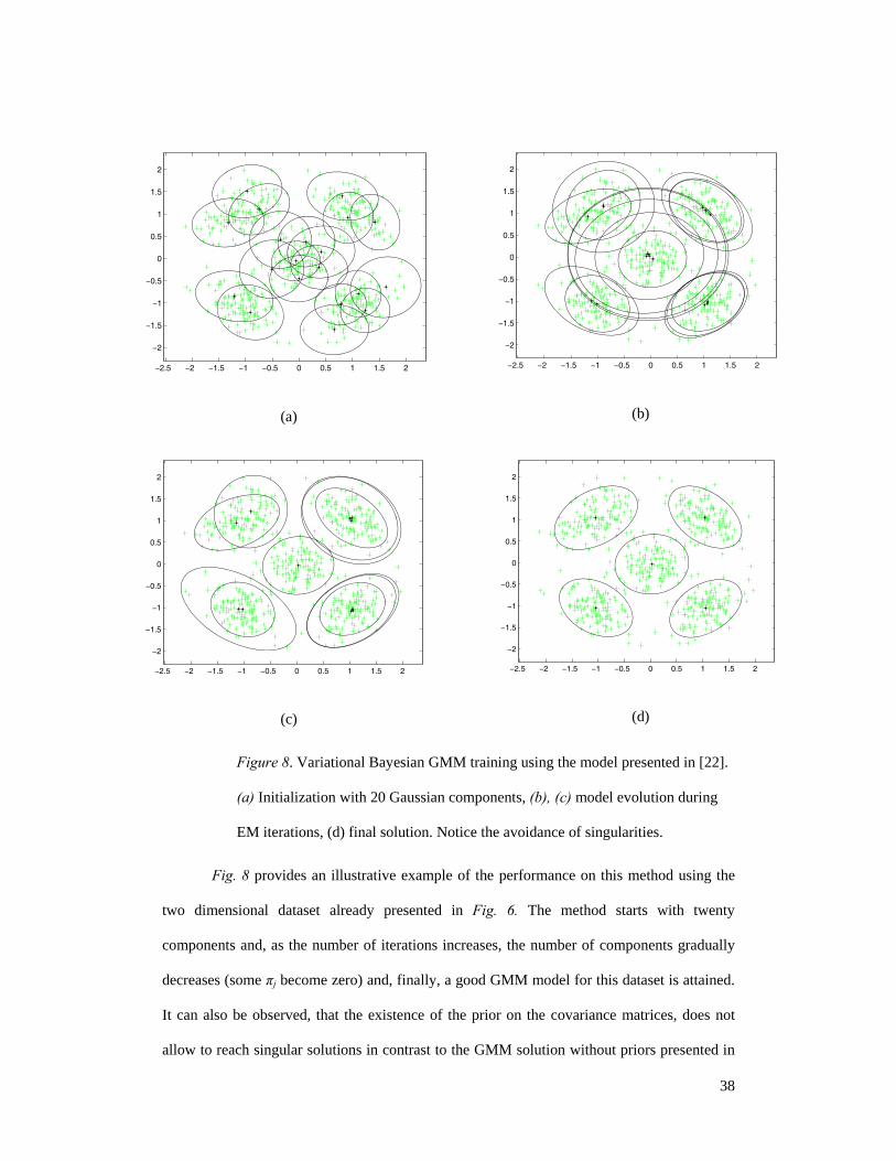
Figure 8. Variational Bayesian GMM training using the model presented in [22].

(a) Initialization with 20 Gaussian components, (b), (c) model evolution during

EM iterations, (d) final solution. Notice the avoidance of singularities.

Fig. 8 provides an illustrative example of the performance on this method using the

two dimensional dataset already presented in Fig. 6. The method starts with twenty

components and, as the number of iterations increases, the number of components gradually

decreases (some πj become zero) and, finally, a good GMM model for this dataset is attained.

It can also be observed, that the existence of the prior on the covariance matrices, does not

allow to reach singular solutions in contrast to the GMM solution without priors presented in

39

Fig. 6.

The CB in general constitutes an effective method exhibiting good performance in the

case where the components are well separated. However its performance exhibits sensitivity

on the specification of the scale matrix V of the Wishart prior imposed on the precision

matrix. In [23] an incremental method for building the above mixture model has been

proposed. At each step learning is restricted in the data region occupied by a specific mixture

component j , thus a local precision prior can be specified based on the precision matrix jT .

In order to achieve this behavior, a modification to the generative model of Fig. 7 was made

that restricts the competition in a subset of the components only.

8. Summary

The EM algorithm is an iterative methodology that offers a number of advantages for

ML estimation. It provides simple iterative solutions, with guaranteed local convergence, for

problems where direct optimization of the likelihood function is difficult. In many cases it

provides solutions that satisfy several constraints for the estimated parameters, for example

covariance matrices are positive definite, probability vectors are positive and sum to one, etc.

Furthermore, the application of EM does not require explicit evaluation of the likelihood

function.

However, in order to apply the EM algorithm we must have knowledge of the

posterior of the hidden variables given the observations. This is a serious drawback since the

EM cannot be applied to complex Bayesian models. However, complex Bayesian models can

be very useful since, if properly constructed, they have the ability to model salient properties

of the data generation mechanism and provide very good solutions to difficult problems.

The variational methodology is an iterative approach that is gaining popularity within

the signal processing community to ameliorate this shortcoming of the EM algorithm.

According to this methodology an approximation to the posterior of the hidden variables

given the observations is used. Based on this approximation Bayesian inference is possible by

40

maximizing a lower bound of the likelihood function which also guarantees local

convergence. This methodology allows inference in the case of complex graphical models,

that in certain cases provide significant improvements as compared to simpler ones that can

be solved via the EM.

This issue was demonstrated in this tutorial paper within the context of linear

regression and Gaussian mixture modeling, which are two fundamental problems for signal

processing applications. More specifically, we demonstrated that complex Bayesian models

that were solved by the variational methodology, in the context of linear regression were able

to better capture local signal properties and avoid ringing in areas of signal discontinuities. In

the context of Gaussian mixture modeling, the models solved by the variational methodology

were able to avoid singularities and to estimate the number of the model components. These

results demonstrate the power of the variational methodology to provide solution to difficult

problems that have plagued signal processing applications for a long time. The main

drawback of this methodology is the lack of results that allow (at least for the time being)

assessing the tightness of the bound that is used.

APPENDIX A: Maximum A Posteriori (MAP): Poor Man’s

Bayesian Inference

One of the most commonly used methodologies in the statistical signal processing

literature is the maximum a posteriori (MAP) method. MAP is often referred to as Bayesian,

since the parameter vector θ is assumed to be a random variable and a prior distribution

( )p θ is imposed on θ . In this appendix we would like to illuminate the similarities and

differences between MAP estimation and Bayesian inference. For x the observation and θ

an unknown quantity the MAP estimate is defined as

( )ˆ argmaxMAP p= |θ

θ θ x . (A.1)

41

Using, Bayes theorem the MAP estimate can be obtained from

ˆ argmax ( ) ( )MAP p p= |θ

θ x θ θ , (A.2)

where ( )p |x θ is the likelihood of the observations. The MAP estimate is easier to obtain

from Eq. (A.2) than (A.1). The posterior in Eq. (A.1) based on Bayes’ theorem is given by

( ) ( )( )

( ) ( )p pp

p p d|

| =|∫

x θ θθ xx θ θ θ

, (A.3)

and requires the computation of the Bayesian integral in the denominator of Eq. (A.3) to

marginalize θ .

From the above it is clear that both MAP and Bayesian estimators assume that θ is a

random variable and use Bayes’ theorem, however, their similarity stops there. For Bayesian

inference the posterior is used and thus θ has to be marginalized. In contrast for MAP the

mode of the posterior is used. One can say that Bayesian inference, unlike MAP averages

over all the available information about θ . Thus, it can be stated that MAP is more like

“poor man’s” Bayesian inference.

The EM can be used to also obtain MAP estimates of θ . Using Bayes’ theorem we

can write

ln ( ) ln ( , ) ln ( ) ln ( | ) ln ( ) ln ( )p p p p p p| = − = + −θ x x θ x x θ θ x . (A.4)

Using a similar framework as for the ML-EM case in Section 4 we can write

( ) ( ) ( ) ( ) ( )( ) ( ) ( )

ln , || ln ln

, ln ln ,

p F q KL q p p p

F q p p

| = + + −

≥ + −

θ x θ θ x

θ θ x (A.5)

where in this context ( )ln p x is a constant. The right hand side of Eq. (A.5) can be

maximized in an alternating fashion as in the EM algorithm. Optimization with respect to

( )q z gives an identical E-step as for the ML case previously explained. Optimization with

respect to θ gives a different M-step since the objective function now contains also the term

( )ln p θ . In general the M-step for the MAP-EM algorithm is more complex than in its ML

counterpart, see for example [26] and [27]. Strictly speaking in such a model MAP estimation

42

is used only for the θ random variables, while Bayesian inference is used for hidden

variables z .

Appendix B: Conjugate Distributions

Conjugate priors play an important role in facilitating Bayesian calculations. More

specifically, assume a Bayesian model with hidden variables z , observed variables x , prior

distribution ( )p z and conditional likelihood ( )p |x z . Then, the marginal likelihood is

given by

( ) ( ) ( ) ( )p p d p p d= , = |∫ ∫x x z z x z z z , (B.1)

which cannot always be computed analytically. The marginalized likelihood is essential in

order to compute the posterior distribution according to ( | ) ( )( | )

( )p pp

p=

x z zz xx

which is

used for Bayesian inference. Thus, it is important to find prior that when multiplied with a

likelihood distribution allows analytical computation of the marginalization integral. A

common practice is to chose the prior distribution such that it has the same form as the

likelihood, so that the resulting posterior distribution has the same form as conditional

likelihood when viewed as a function of the hidden variable. Such prior distributions allow

closed form marginalization of the hidden variables and are said to be conjugate to the

likelihood distribution.

For example consider a Gaussian conditional likelihood zero mean with hidden

variable α the precision ( ) ( )11 222 1( | ) 2 exp 2p x xα π α α−

= − . This likelihood when

viewed as a function of α has the form of a Gamma pdf given

by( ) ( )1( ; , ) exp

aabp z a b z zb

a−= −

Γ. Thus, the marginalization of the precision of a Gaussian

pdf when a Gamma conjugate prior is used for it is doable in closed form according to

43

( ) ( ) ( )( )( ) ( )

( )12 2

12

12; , / ; , ,

22

aaa b xp x a b p z p a b da ba

α απ

− +Γ + ⎛ ⎞= = +⎜ ⎟Γ ⎝ ⎠∫ (B.2)

and gives the well known Student-t pdf.

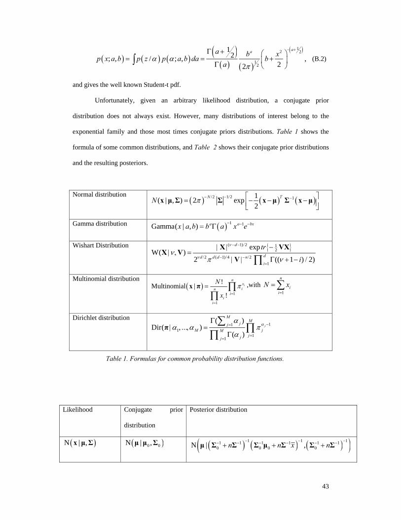
Unfortunately, given an arbitrary likelihood distribution, a conjugate prior

distribution does not always exist. However, many distributions of interest belong to the

exponential family and those most times conjugate priors distributions. Table 1 shows the

formula of some common distributions, and Table 2 shows their conjugate prior distributions

and the resulting posteriors.

Normal distribution ( ) ( ) ( )1/2/2 11( | , ) 2 exp

2N TN π −− −⎡ ⎤= − − −⎢ ⎥⎣ ⎦

x μ Σ Σ x μ Σ x μ

Gamma distribution ( ) 1 1Gamma( | , ) a a bxx a b b a x e− − −= Γ

Wishart Distribution { }( 1) 2 12

2 ( 1) 4 21

expW( )

2 (( 1 ) 2)

d

dd d d ni

tr

i

ν

νν

π ν

− − /

/ − / − /=

| | −| , =

| | Γ + − /∏X VX

X VV

Multinomial distribution ( )

1

1

!Multinomial |!

i

nxin

ii

i

N

xπ

=

=

= ∏∏

x π ,with 1

n

ii

N x=

=∑

Dirichlet distribution 11

11

1

( )Dir( )

( )j

MMjj

M jMjjj

… ααα α π

α−=

==

Γ| , , =

Γ

∑∏

∏π

Table 1. Formulas for common probability distribution functions.

Likelihood Conjugate prior

distribution

Posterior distribution

( )N | ,x μ Σ ( )0 0N | ,μ μ Σ ( ) ( ) ( )( )1 1 11 1 1 1 1 10 0 0 0N | ,n n x n

− − −− − − − − −+ + +μ Σ Σ Σ μ Σ Σ Σ

44

( )2N | ,x μ σ 2Gamma( | , )a bσ − ( )2 21

Gamma | / 2, ( ) / 2nii

a n b xσ μ−=

+ + −∑

( )N | ,x μ Σ ( )1Wishart | ,ν−Σ V ( ) ( )( )11

Wishart | , n Ti ii

nν−=

+ + − −∑Σ V x μ x μ

( )Multinomial |x π Dir( | )π a 1

Dir( | )nii

x=

+∑π a

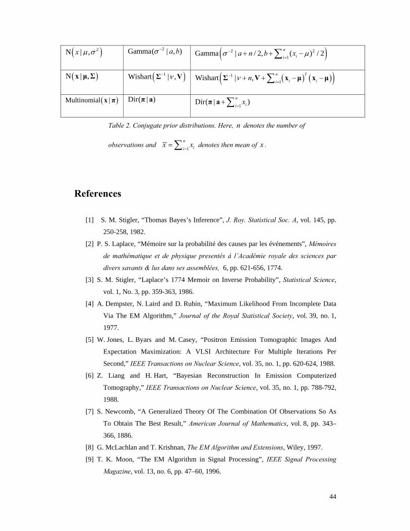
Table 2. Conjugate prior distributions. Here, n denotes the number of

observations and 1

nii

x x=

= ∑ denotes then mean of x .

References

[1] S. M. Stigler, “Thomas Bayes’s Inference”, J. Roy. Statistical Soc. A, vol. 145, pp.

250-258, 1982.

[2] P. S. Laplace, “Mémoire sur la probabilité des causes par les événements”, Mémoires

de mathématique et de physique presentés á l’Académie royale des sciences par

divers savants & lus dans ses assemblées, 6, pp. 621-656, 1774.

[3] S. M. Stigler, “Laplace’s 1774 Memoir on Inverse Probability”, Statistical Science,

vol. 1, No. 3, pp. 359-363, 1986.

[4] A. Dempster, N. Laird and D. Rubin, “Maximum Likelihood From Incomplete Data

Via The EM Algorithm,” Journal of the Royal Statistical Society, vol. 39, no. 1,

1977.

[5] W. Jones, L. Byars and M. Casey, “Positron Emission Tomographic Images And

Expectation Maximization: A VLSI Architecture For Multiple Iterations Per

Second,” IEEE Transactions on Nuclear Science, vol. 35, no. 1, pp. 620-624, 1988.

[6] Z. Liang and H. Hart, “Bayesian Reconstruction In Emission Computerized

Tomography,” IEEE Transactions on Nuclear Science, vol. 35, no. 1, pp. 788-792,

1988.

[7] S. Newcomb, “A Generalized Theory Of The Combination Of Observations So As

To Obtain The Best Result,” American Journal of Mathematics, vol. 8, pp. 343–

366, 1886.

[8] G. McLachlan and T. Krishnan, The EM Algorithm and Extensions, Wiley, 1997.

[9] T. K. Moon, “The EM Algorithm in Signal Processing”, IEEE Signal Processing

Magazine, vol. 13, no. 6, pp. 47–60, 1996.

45

[10] R. M. Neal and G. E. Hinton, “A View Of The EM Algorithm That Justifies

Incremental, Sparse And Other Variants,” in Learning in Graphical Models, M. I.

Jordan, Ed, pp. 355–368, MIT Press, 1998.

[11] M. N. Gibbs and D. J. C. Mackay, “Variational Gaussian Process Classifiers”,

IEEE Trans. Neural Networks, vol. 11 , no. 6, pp. 1458 – 1464, Nov. 2000.

[12] S. Waterhouse, D. McKay, T. Robinson, “Bayesian Methods for Mixtures of

Experts”, Advances in Neural Information Processing Systems 8, D. S. Touretzky,

M. Mozer, M. E. Hasselmo (Eds.), pp. 351-357, MIT Press 1996.

[13] C. Bishop, Pattern Recognition and Machine Learning, Springer Verlag, 2006.

[14] C. Robert and G. Cassela, Monte Carlo Statistical Methods, Springer Verlag, 1999.

[15] C. Andrieu, N. de Freitas, A. Doucet and M. Jordan, “An Introduction To MCMC

For Machine Learning”, Machine Learning, vol. 50, pp. 5–43, 2003.

[16] S. M. Kay, Fundamentals of Statistical Signal Processing: Estimation Theory,

Prentice-Hall, 1993.

[17] A. Likas, N.P. Galatsanos, “A Variational Approach For Bayesian Blind Image

Deconvolution”, IEEE Transactions on Signal Processing, vol. 52, no. 8, p. 2222–

2233, Aug 2004.

[18] R. Weinstock, Calculus of Variations, Dover Publications, 1974.

[19] T. S. Jaakkola, Variational Methods for Inference and Learning in Graphical

Models, Ph.D. Thesis, MIT, 1997.

[20] M. Jordan, Z. Gharamani, T. Jaakkola, and L. Saul, “An Introduction To

Variational Methods For Graphical Models,” in Learning in Graphical Models,

M. Jordan, Ed., pp. 105–162, MIT Press, 1998.

[21] G. Parisi, Statistical Field Theory, Addison-Wesley, 1988.

[22] A. Corduneanu and C. Bishop, “Variational Bayesian Model Selection for Mixture

Distributions“, Proc. AI and Statistics Conference, January 2001

[23] C. Constantinopoulos and A. Likas, "Unsupervised Learning of Gaussian Mixtures

Based on Variational Component Splitting", IEEE Trans. on Neural Networks, vol.

18, no.2, pp. 745-755, March 2007.

[24] C. Borgelt and R. Kruse, Graphical Models Methods for Data Analysis and

Mining, Wiley, 2002.

[25] R. Neapolitan, Learning Bayesian Networks, Prentice Hall, 2004.

[26] K. Blekas, A. Likas, N. Galatsanos and I. E. Lagaris. "A Spatially-Constrained

Mixture Model for Image Segmentation". IEEE Transactions on Neural Networks,

vol. 16, no 2, pp. 494-498, 2005.

[27] C. Nikou, N. Galatsanos, and A. Likas, "A Class-Adaptive Spatially Variant

Mixture Model for Image Segmentation", IEEE Trans. on Image Processing, Vol.

46

16, No. 4, pp. 1121-1130, April 2007.

[28] V. Smídl, A. Quinn, The Variational Bayes Method in Signal Processing, Springer,

2005.

[29] C. Bishop, M. Tipping, “Variational Relevance Vector Machines”, Proc. of the

16th Conference on Uncertainty in Artificial Intelligence, pp. 46-53, 2000.

[30] H. Attias, "A Variational Bayesian Framework for Graphical Models", Proc. NIPS

12, pp. 209-216, MIT Press, 2000.

[31] Watanabe, S.; Minami, Y.; Nakamura, A.; Ueda, N.; “Variational Bayesian

estimation and clustering for speech recognition”, IEEE Transactions on Speech

and Audio Processing, Volume 12, Issue 4, Page(s):365 – 381, July 2004.

[32] Watanabe, S.; Sako, A.; Nakamura, A., “Automatic determination of acoustic

model topology using variational Bayesian estimation and clustering for large

vocabulary continuous speech recognition”, IEEE Transactions on Audio, Speech

and Language Processing, Volume 14, Issue 3, Page(s):855 – 872, May 2006.

[33] Oh-Wook Kwon; Kwokleung Chan; Te-Won Lee; “Speech feature analysis using

variational Bayesian PCA”, IEEE Signal Processing Letters, Volume 10, Issue 5,

Page(s):137 – 140, May 2003.

[34] Sykacek, P.; Roberts, S.J.; Stokes, M.; “Adaptive BCI based on variational

Bayesian Kalman filtering: an empirical evaluation”, IEEE Transactions on

Biomedical Engineering, Volume 51, Issue 5, May 2004 Page(s):719 – 727

[35] Roberts, S.J.; Penny, W.D.; “Variational Bayes for generalized autoregressive

models”, IEEE Transactions on Signal Processing, Volume 50, Issue 9, Sept.

2002 Page(s):2245 – 2257

[36] Molina, R.; Mateos, J.; Katsaggelos, A. K.; “Blind Deconvolution Using a

Variational Approach to Parameter, Image and Blur Estimation”, IEEE

Transactions on Image Processing, Volume 15, Issue 12, Page(s):3715 – 3727,

Dec. 2006.

[37] D. Tzikas, A. Likas, and N. Galatsanos, “Variational Bayesian Blind Image

Deconvolution with Student-T Priors”, IEEE International Conference on Image

Processing, (ICIP), Volume 1, Page(s): I - 109 - I – 112, September 2007.

[38] Babacan, S. D.; Molina, R.; Katsaggelos, A. K.; “Total Variation Image

Restoration and Parameter Estimation using Variational Posterior Distribution

Approximation”, IEEE International Conference on Image Processing, Volume 1,

Page(s):I - 97 - I – 100, September 2007.

[39] Chantas, G.; Galatsanos, N.; Likas, A.; “Bayesian Image Restoration Based On

Variatonal Inference and a Product of Student-t Priors”, IEEE Workshop on

Machine Learning for Signal Processing, Page(s):93 – 98, Aug. 2007