Lie Groups - Department of Physics | CoAS | Drexel …bob/LieGroups/LG_01.pdf · Lie Groups Robert...
34
Lie Groups Robert Gilmore
Transcript of Lie Groups - Department of Physics | CoAS | Drexel …bob/LieGroups/LG_01.pdf · Lie Groups Robert...

Lie Groups
Robert Gilmore

iii
Many years ago I wrote the book Lie Groups, Lie Algebras, and Some
of Their Applications (NY: Wiley, 1974). That was a big book: long
and difficult. Over the course of the years I realized that more than
90% of the most useful material in that book could be presented in less
than 10% of the space. This realization was accompanied by a promise
that some day I would do just that — rewrite and shrink the book to
emphasize the most useful aspects in a way that was easy for students to
acquire and to assimilate. The present work is the fruit of this promise.
In carrying out the revision I’ve created a sandwich. Lie group theory
has its intellectual underpinnings in Galois theory. In fact, the original
purpose of what we now call Lie group theory was to use continuous
groups to solve differential (continuous) equations in the spirit that finite
groups had been used to solve algebraic (finite) equations. It is rare
that a book dedicated to Lie groups begins with Galois groups and
includes a chapter dedicated to the applications of Lie group theory
to solving differential equations. This book does just that. The first
chapter describes Galois theory, and the last chapter shows how to use
Lie theory to solve some ordinary differential equations. The fourteen
intermediate chapters describe many of the most important aspects of
Lie group theory and provide applications of this beautiful subject to
several important areas of physics and geometry.
Over the years I have profitted from the interaction with many stu-
dents through comments, criticism, and suggestions for new material
or different approaches to old. Three students who have contributed
enormously during the past few years are Dr. Jairzinho Ramos-Medina,
who worked with me on Chapter 15 (Maxwell’s Equations), and Daniel
J. Cross and Timothy Jones, who aided this computer illiterate with
much moral and ebit ether support. Finally, I thank my beautiful wife
Claire for her gracious patience and understanding throughout this long
creation process.
Contents
1 Introduction page 1
1.1 The Program of Lie 1
1.2 A Result of Galois 3
1.3 Group Theory Background 4
1.4 Approach to Solving Polynomial Equations 9
1.5 Solution of the Quadratic Equation 10
1.6 Solution of the Cubic Equation 12
1.7 Solution of the Quartic Equation 15
1.8 The Quintic Cannot be Solved 18
1.9 Example 19
1.10 Conclusion 22
1.11 Problems 23
2 Lie Groups 25
2.1 Algebraic Properties 25
2.2 Topological Properties 27
2.3 Unification of Algebra and Topology 29
2.4 Unexpected Simplification 31
2.5 Conclusion 31
2.6 Problems 32
3 Matrix Groups 37
3.1 Preliminaries 37
3.2 No Constraints 39
3.3 Linear Constraints 39
3.4 Bilinear and Quadratic Constraints 42
3.5 Multilinear Constraints 46
3.6 Intersections of Groups 46
3.7 Embedded Groups 47
iv

Contents v
3.8 Modular Groups 48
3.9 Conclusion 50
3.10 Problems 50
4 Lie Algebras 61
4.1 Why Bother? 61
4.2 How to Linearize a Lie Group 63
4.3 Inversion of the Linearization Map: EXP 64
4.4 Properties of a Lie Algebra 66
4.5 Structure Constants 68
4.6 Regular Representation 69
4.7 Structure of a Lie Algebra 70
4.8 Inner Product 71
4.9 Invariant Metric and Measure on a Lie Group 74
4.10 Conclusion 76
4.11 Problems 76
5 Matrix Algebras 82
5.1 Preliminaries 82
5.2 No Constraints 83
5.3 Linear Constraints 83
5.4 Bilinear and Quadratic Constraints 86
5.5 Multilinear Constraints 89
5.6 Intersections of Groups 89
5.7 Algebras of Embedded Groups 90
5.8 Modular Groups 91
5.9 Basis Vectors 91
5.10 Conclusion 93
5.11 Problems 93
6 Operator Algebras 98
6.1 Boson Operator Algebras 98
6.2 Fermion Operator Algebras 99
6.3 First Order Differential Operator Algebras 100
6.4 Conclusion 103
6.5 Problems 104
7 EXPonentiation 110
7.1 Preliminaries 110
7.2 The Covering Problem 111
7.3 The Isomorphism Problem and the Covering Group 116
7.4 The Parameterization Problem and BCH Formulas 121
7.5 EXPonentials and Physics 127

vi Contents
7.5.1 Dynamics 127
7.5.2 Equilibrium Thermodynamics 129
7.6 Conclusion 132
7.7 Problems 133
8 Structure Theory for Lie Algebras 145
8.1 Regular Representation 145
8.2 Some Standard Forms for the Regular Representation 146
8.3 What These Forms Mean 149
8.4 How to Make This Decomposition 152
8.5 An Example 153
8.6 Conclusion 154
8.7 Problems 154
9 Structure Theory for Simple Lie Algebras 157
9.1 Objectives of This Program 157
9.2 Eigenoperator Decomposition – Secular Equation 158
9.3 Rank 161
9.4 Invariant Operators 161
9.5 Regular Elements 164
9.6 Semisimple Lie algebras 166
9.6.1 Rank 166
9.6.2 Properties of Roots 166
9.6.3 Structure Constants 168
9.6.4 Root Reflections 169
9.7 Canonical Commutation Relations 169
9.8 Conclusion 171
9.9 Problems 173
10 Root Spaces and Dynkin Diagrams 179
10.1 Properties of Roots 179
10.2 Root Space Diagrams 181
10.3 Dynkin Diagrams 185
10.4 Conclusion 189
10.5 Problems 191
11 Real Forms 194
11.1 Preliminaries 194
11.2 Compact and Least Compact Real Forms 197
11.3 Cartan’s Procedure for Constructing Real Forms 199
11.4 Real Forms of Simple Matrix Lie Algebras 200
11.4.1 Block Matrix Decomposition 201
11.4.2 Subfield Restriction 201
Contents vii
11.4.3 Field Embeddings 204
11.5 Results 204
11.6 Conclusion 205
11.7 Problems 206
12 Riemannian Symmetric Spaces 213
12.1 Brief Review 213
12.2 Globally Symmetric Spaces 215
12.3 Rank 216
12.4 Riemannian Symmetric Spaces 217
12.5 Metric and Measure 218
12.6 Applications and Examples 219
12.7 Pseudo Riemannian Symmetic Spaces 222
12.8 Conclusion 223
12.9 Problems 224
13 Contraction 232
13.1 Preliminaries 233
13.2 Inonu–Wigner Contractions 233
13.3 Simple Examples of Inonu–Wigner Contractions 234
13.3.1 The Contraction SO(3) → ISO(2) 234
13.3.2 The Contraction SO(4) → ISO(3) 235
13.3.3 The Contraction SO(4, 1) → ISO(3, 1) 237
13.4 The Contraction U(2) → H4 239
13.4.1 Contraction of the Algebra 239
13.4.2 Contraction of the Casimir Operators 240
13.4.3 Contraction of the Parameter Space 240
13.4.4 Contraction of Representations 241
13.4.5 Contraction of Basis States 241
13.4.6 Contraction of Matrix Elements 242
13.4.7 Contraction of BCH Formulas 242
13.4.8 Contraction of Special Functions 243
13.5 Conclusion 244
13.6 Problems 245
14 Hydrogenic Atoms 250
14.1 Introduction 251
14.2 Two Important Principals of Physics 252
14.3 The Wave Equations 253
14.4 Quantization Conditions 254
14.5 Geometric Symmetry SO(3) 257
14.6 Dynamical Symmetry SO(4) 261
viii Contents
14.7 Relation With Dynamics in Four Dimensions 264
14.8 DeSitter Symmetry SO(4, 1) 266
14.9 Conformal Symmetry SO(4, 2) 270
14.9.1 Schwinger Representation 270
14.9.2 Dynamical Mappings 271
14.9.3 Lie Algebra of Physical Operators 274
14.10 Spin Angular Momentum 275
14.11 Spectrum Generating Group 277
14.11.1 Bound States 278
14.11.2 Scattering States 279
14.11.3 Quantum Defect 280
14.12 Conclusion 281
14.13 Problems 282
15 Maxwell’s Equations 293
15.1 Introduction 294
15.2 Review of the Inhomogeneous Lorentz Group 295
15.2.1 Homogeneous Lorentz Group 295
15.2.2 Inhomogeneous Lorentz Group 296
15.3 Subgroups and Their Representations 296
15.3.1 Translations {I, a} 297
15.3.2 Homogeneous Lorentz Transformations 297
15.3.3 Representations of SO(3, 1) 298
15.4 Representations of the Poincare Group 299
15.4.1 Manifestly Covariant Representations 299
15.4.2 Unitary Irreducible Representations 300
15.5 Transformation Properties 305
15.6 Maxwell’s Equations 308
15.7 Conclusion 309
15.8 Problems 310
16 Lie Groups and Differential Equations 320
16.1 The Simplest Case 322
16.2 First Order Equations 323
16.2.1 One Parameter Group 323
16.2.2 First Prolongation 323
16.2.3 Determining Equation 324
16.2.4 New Coordinates 325
16.2.5 Surface and Constraint Equations 326
16.2.6 Solution in New Coordinates 327
16.2.7 Solution in Original Coordinates 327
Contents ix
16.3 An Example 327
16.4 Additional Insights 332
16.4.1 Other Equations, Same Symmetry 332
16.4.2 Higher Degree Equations 333
16.4.3 Other Symmetries 333
16.4.4 Second Order Equations 333
16.4.5 Reduction of Order 335
16.4.6 Higher Order Equations 336
16.4.7 Partial Differential Equations: Laplace’s
Equation 337
16.4.8 Partial Differential Equations: Heat Equation338
16.4.9 Closing Remarks 338
16.5 Conclusion 339
16.6 Problems 341
Bibliography 347
Index 351


1
Introduction
Contents
1.1 The Program of Lie 11.2 A Result of Galois 31.3 Group Theory Background 41.4 Approach to Solving Polynomial
Equations 91.5 Solution of the Quadratic Equation 101.6 Solution of the Cubic Equation 121.7 Solution of the Quartic Equation 151.8 The Quintic Cannot be Solved 181.9 Example 191.10 Conclusion 221.11 Problems 23
Lie groups were initially introduced as a tool to solve or simplify ordinaryand partial differential equations. The model for this application wasGalois’ use of finite groups to solve algebraic equations of degree two,three, and four, and to show that the general polynomial equation ofdegree greater than four could not be solved by radicals. In this chapterwe show how the structure of the finite group that leaves a quadratic,cubic, or quartic equation invariant can be used to develop an algorithmto solve that equation.
1.1 The Program of Lie
Marius Sophus Lie (1842 - 1899) embarked on a program that is still not
complete, even after a century of active work. This program attempts
to use the power of the tool called group theory to solve, or at least
simplify, ordinary differential equations.
Earlier in that century, Evariste Galois (1811 - 1832) had used group
theory to solve algebraic (polynomial) equations that were quadratic,
cubic, and quartic. In fact, he did more. He was able to prove that
1
2 Introduction
no closed form solution could be constructed for the general quintic (or
any higher degree) equation using only the four standard operations of
arithmetic (+,−,×,÷) as well as extraction of the nth roots of a complex
number.
Lie initiated his program on the basis of analogy. If finite groups
were required to decide on the solvability of finite-degree polynomial
equations, then ‘infinite groups’ (i.e., groups depending continuously on
one or more real or complex variables) would probably be involved in
the treatment of ordinary and partial differential equations. Further, Lie
knew that the structure of the polynomial’s invariance (Galois) group
not only determined whether the equation was solvable in closed form,
but also provided the algorithm for constructing the solution in the case
that the equation was solvable. He therefore felt that the structure
of an ordinary differential equation’s invariance group would determine
whether or not the equation could be solved or simplified and, if so, the
group’s structure would also provide the algorithm for constructing the
solution or simplification.
Lie therefore set about the program of computing the invariance group
of ordinary differential equations. He also began studying the structure
of the children he begat, which we now call Lie groups.
Lie groups come in two basic varieties: the simple and the solvable.
Simple groups have the property that they regenerate themselves under
commutation. Solvable groups do not, and contain a chain of subgroups,
each of which is an invariant subgroup of its predecessor.
Simple and solvable groups are the building blocks for all other Lie
groups. Semisimple Lie groups are direct products of simple Lie groups.
Nonsemisimple Lie groups are semidirect products of (semi)simple Lie
groups with invariant subgroups that are solvable.
Not surprisingly, solvable Lie groups are related to the integrability, or
at least simplification, of ordinary differential equations. However, sim-
ple Lie groups are more rigidly constrained, and form such a beautiful
subject of study in their own right that much of the effort of mathe-
maticians during the last century involved the classification and com-
plete enumeration of all simple Lie groups and the discussion of their
properties. Even today, there is no complete classification of solvable
Lie groups, and therefore nonsemisimple Lie groups.
Both simple and solvable Lie groups play an important role in the
study of differential equations. As in Galois’ case of polynomial equa-
tions, differential equations can be solved or simplified by quadrature if
their invariance group is solvable. On the other hand, most of the classi-

1.2 A Result of Galois 3
cal functions of mathematical physics are matrix elements of simple Lie
groups in particular matrix representations. There is a very rich con-
nection between Lie groups and special functions that is still evolving.
1.2 A Result of Galois
In 1830 Galois developed machinery that allowed mathematicians to
definitively resolve questions that had eluded answers for 2000 years or
longer. These questions included the three famous challenges to ancient
Greek geometers: Whether by ruler and compasses alone it was possible
to
• square a circle
• trisect an angle
• double a cube.
His work helped to resolve longstanding questions of an algebraic nature:
Whether it was possible, using only the operations of arithmetic together
with the operation of constructing radicals, to solve
• cubic equations
• quartic equations
• quintic equations.
This branch of mathematics, now called Galois theory, continues to pro-
vide powerful new results, such as supplying answers and solution meth-
ods to the following questions:
• Can an algebraic expression be integrated in closed form?
• Under what conditions can errors in a binary code be corrected?
This beautiful machine, applied to a problem, provides important re-
sults. First, it can determine whether a solution is possible or not under
the conditions specified. Second, if a solution is possible, it suggests the
structure of the algorithm that can be used to construct the solution in
a finite number of well-defined steps.
Galois’ approach to the study of algebraic (polynomial) equations in-
volved two areas of mathematics, now called field theory and group
theory. One useful statement of Galois’ result is [50, 66]:
Theorem: A polynomial equation over the complex field is solvable
by radicals if and only if its Galois group G contains a chain of subgroups
G = G0 ⊃ G1 ⊃ · · · ⊃ Gω = I with the properties:
4 Introduction
1. Gi+1 is an invariant subgroup of Gi;
2. Each factor group Gi/Gi+1 is commutative.
In the statement of this theorem the field theory niceties are contained
in the term ‘solvable by radicals.’ This means that in addition to the four
standard arithmetic operations +,−,×,÷ one is allowed the operation
of taking nth roots of complex numbers.
The principal result of this theorem is stated in terms of the structure
of the group that permutes the roots of the polynomial equation among
themselves. Determining the structure of this group is a finite, and in
fact very simple, process.
1.3 Group Theory Background
A group G is defined as follows: It consists of a set of operations
G = {g1, g2, . . . }, called group operations, together with a combina-
torial operation, ·, called group multiplication, such that the following
four axioms are satisfied:
(i) Closure: If gi ∈ G, gj ∈ G, then gi · gj ∈ G.
(ii) Associativity: for all gi ∈ G, gj ∈ G, gk ∈ G,
(gi · gj) · gk = gi · (gj · gk)
(iii) Identity: There is a group operation, I (identity operator), with
the property that
gi · I = gi = I · gi
(iv) Inverse: Every group operation gi has an inverse (called g−1i ):
gi · g−1i = I = g−1
i · gi
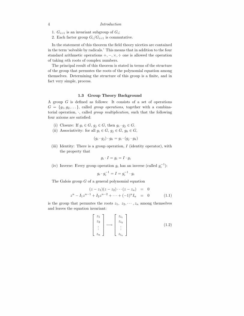
The Galois group G of a general polynomial equation
(z − z1)(z − z2) · · · (z − zn) = 0
zn − I1zn−1 + I2z
n−2 + · · · + (−1)nIn = 0 (1.1)
is the group that permutes the roots z1, z2, · · · , zn among themselves
and leaves the equation invariant:
z1
z2
...
zn
−→
zi1
zi2...
zin
(1.2)
1.3 Group Theory Background 5
This group, called the permutation group Pn or the symmetric group
Sn, has n! group operations. Each group operation is some permutation
of the roots of the polynomial; the group multiplication is composition
of successive permutations.
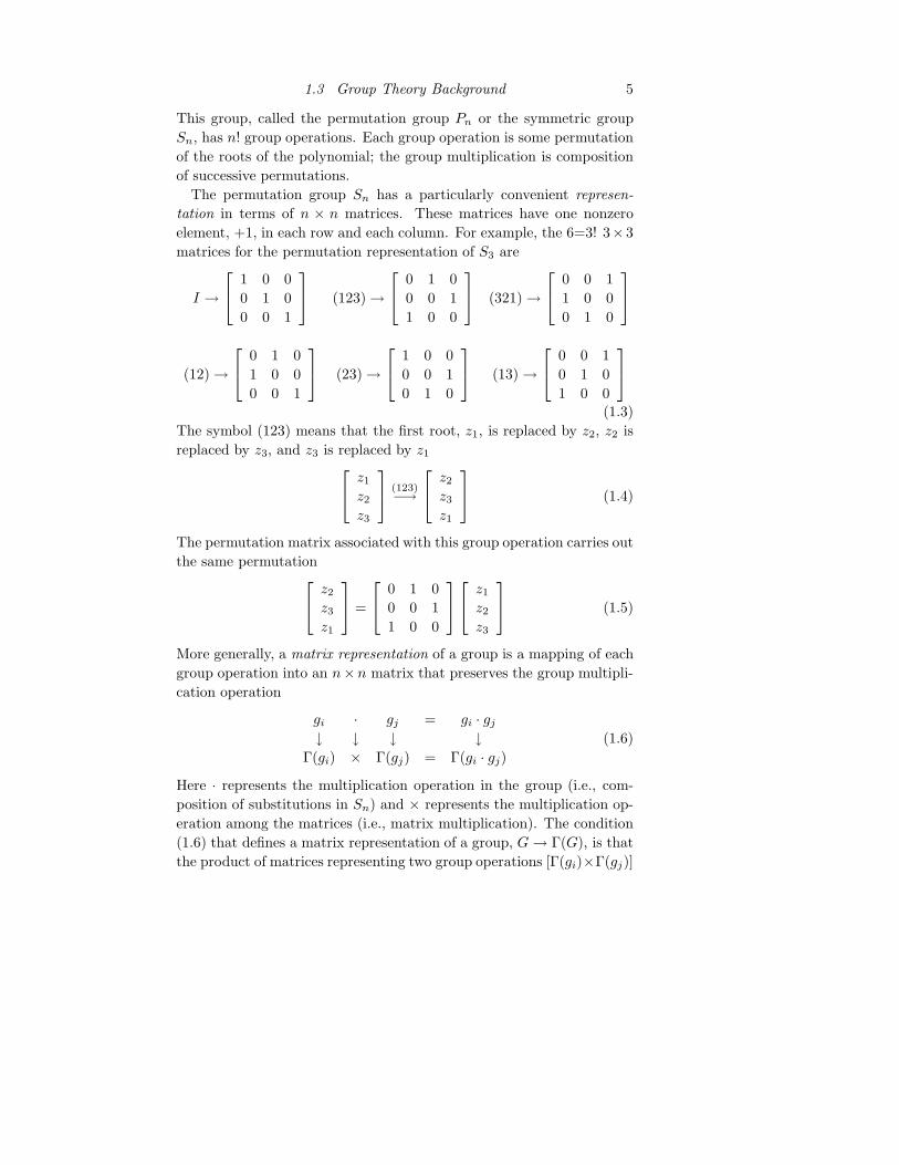
The permutation group Sn has a particularly convenient represen-
tation in terms of n × n matrices. These matrices have one nonzero
element, +1, in each row and each column. For example, the 6=3! 3×3
matrices for the permutation representation of S3 are
I →
1 0 0
0 1 0
0 0 1
(123) →
0 1 0
0 0 1
1 0 0
(321) →
0 0 1
1 0 0
0 1 0
(12) →
0 1 0
1 0 0
0 0 1
(23) →
1 0 0
0 0 1
0 1 0
(13) →
0 0 1
0 1 0
1 0 0
(1.3)
The symbol (123) means that the first root, z1, is replaced by z2, z2 is
replaced by z3, and z3 is replaced by z1
z1
z2
z3
(123)−→
z2
z3
z1
(1.4)
The permutation matrix associated with this group operation carries out
the same permutation
z2
z3
z1
=
0 1 0
0 0 1
1 0 0
z1
z2
z3
(1.5)
More generally, a matrix representation of a group is a mapping of each
group operation into an n×n matrix that preserves the group multipli-
cation operation
gi · gj = gi · gj
↓ ↓ ↓ ↓Γ(gi) × Γ(gj) = Γ(gi · gj)
(1.6)
Here · represents the multiplication operation in the group (i.e., com-
position of substitutions in Sn) and × represents the multiplication op-
eration among the matrices (i.e., matrix multiplication). The condition
(1.6) that defines a matrix representation of a group, G → Γ(G), is that
the product of matrices representing two group operations [Γ(gi)×Γ(gj)]
6 Introduction
is equal to the matrix representing the product of these operations in
the group [Γ(gi · gj)] for all group operations gi, gj ∈ G.
This permutation representation of S3 is 1:1, or a faithful representa-
tion of S3, since knowledge of the 3 × 3 matrix uniquely identifies the
original group operation in S3.
A subgroup H of the group G is a subset of group operations in G that
is closed under the group multiplication in G.
Example: The subset of operations I, (123), (321) forms a subgroup
of S3. This particular subgroup is denoted A3 (alternating group). It
consists of those operations in S3 whose determinants, in the permuta-
tion representation, are +1. The group S3 has three two-element sub-
groups:
S2(12) = {I, (12)}S2(23) = {I, (23)}S2(13) = {I, (13)}
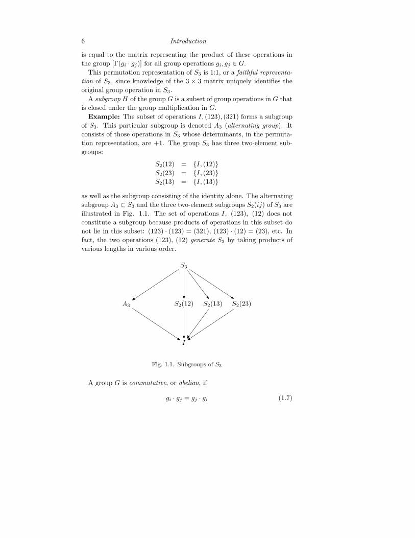
as well as the subgroup consisting of the identity alone. The alternating
subgroup A3 ⊂ S3 and the three two-element subgroups S2(ij) of S3 are
illustrated in Fig. 1.1. The set of operations I, (123), (12) does not
constitute a subgroup because products of operations in this subset do
not lie in this subset: (123) · (123) = (321), (123) · (12) = (23), etc. In
fact, the two operations (123), (12) generate S3 by taking products of
various lengths in various order.
S3
A3 S2(12) S2(13) S2(23)
I
Fig. 1.1. Subgroups of S3
A group G is commutative, or abelian, if
gi · gj = gj · gi (1.7)
1.3 Group Theory Background 7
for all group operations gi, gj ∈ G.
Example: S3 is not commutative, while A3 is. For S3 we have
(12)(23) = (321)
(123) 6= (321)
(23)(12) = (123)
(1.8)
Two subgroups of G, H1 ⊂ G and H2 ⊂ G are conjugate if there is a
group element g ∈ G with the property
gH1g−1 = H2 (1.9)
Example: The subgroups S2(12) and S2(13) are conjugate in S3 since
(23)S2(12)(23)−1 = (23) {I, (12)} (23)−1 = {I, (13)} = S2(13) (1.10)
On the other hand, the alternating group A3 ⊂ S3 is self-conjugate, since
any operation in G = S3 serves merely to permute the group operations
in A3 among themselves:
(23)A3(23)−1 = (23) {I, (123), (321)} (23)−1 = {I, (321), (123)} = A3
(1.11)
A subgroup H ⊂ G which is self-conjugate under all operations in G
is called an invariant subgroup of G, or normal subgroup of G.
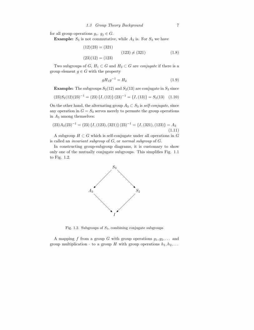
In constructing group-subgroup diagrams, it is customary to show
only one of the mutually conjugate subgroups. This simplifies Fig. 1.1
to Fig. 1.2.
S3
A3 S2
I
Fig. 1.2. Subgroups of S3, combining conjugate subgroups
A mapping f from a group G with group operations g1, g2, . . . and
group multiplication · to a group H with group operations h1, h2, . . .

8 Introduction
and group multiplication × is called a homomorphism if it preserves
group multiplication:
gi · gj = gi · gj
↓ ↓ ↓ ↓f(gi) × f(gj) = f(gi · gj)
(1.12)
The group H is called a homomorphic image of G. Several different
group elements in G may map to a single group element in H . Every
element hi ∈ H has the same number of inverse images gj ∈ G. If each
group element h ∈ H has a unique inverse image g ∈ G (h1 = f(g1) and
h2 = f(g2), h1 = h2 ⇒ g1 = g2) the mapping f is an isomorphism.
Example: The 3:1 mapping f of S3 onto S2 given by
S3f−→ S2
I, (123), (321) −→ I
(12), (23), (31) −→ (12)
(1.13)
is a homomorphism.
Example: The 1:1 mapping of S3 onto the six 3 × 3 matrices given
in (1.3) is an isomorphism.
Remark: Homomorphisms of groups to matrix groups, such as that
in (1.3), are called matrix representations. The representation in (1.3)
is 1:1 or faithful, since the mapping is an isomorphism.
Remark: Isomorphic groups are indistinguishable at the algebraic
level. Thus, when an isomorphism exists between a group and a matrix
group, it is often preferable to study the matrix representation of the
group since the properties of matrices are so well known and familiar.
This is the approach we pursue in Chapter 3 when discussing Lie groups.
If H is a subgroup of G, it is possible to write every group element in
G as a product of an element h in the subgroup H with a group element
in a ‘quotient,’ or coset (denoted G/H). A coset is a subset of G. If the
order of G is |G| (S3 has 3! = 6 group elements, so the order of S3 is 6),
then the order of G/H is |G/H | = |G|/|H |. For example, for subgroups
H = A3 = {I, (123), (321)} and H = S2(23) = {I, (23)} we have
G/H · H = G
{I, (12)} · {I, (123), (321)} = {I, (123), (321), (12), (13), (23)}{I, (12), (321)} · {I, (23)} = {I, (23), (12), (123), (321), (13)}
(1.14)
The choice of the |G|/|H | group elements in the quotient space is not
unique. For the subgroup A3 we could equally well have chosen G/H =
1.4 Approach to Solving Polynomial Equations 9
S3/A3 = {I, (13)} or {I, (23)}; for S2(23) we could equally well have
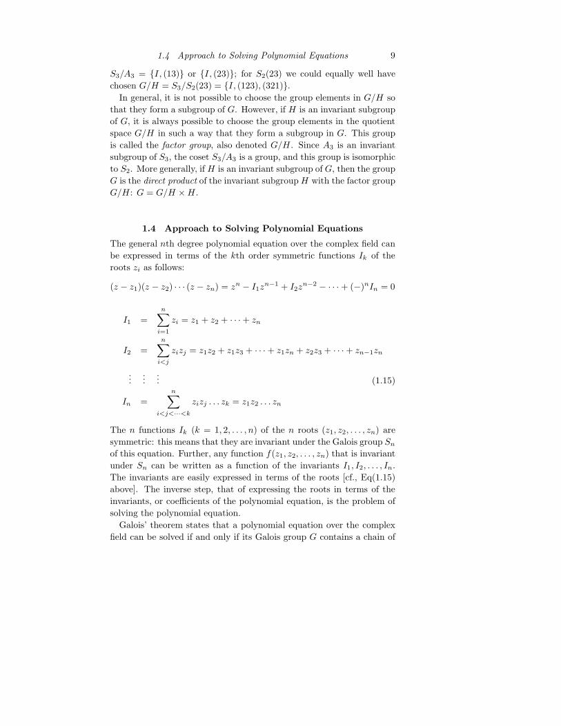
chosen G/H = S3/S2(23) = {I, (123), (321)}.In general, it is not possible to choose the group elements in G/H so
that they form a subgroup of G. However, if H is an invariant subgroup
of G, it is always possible to choose the group elements in the quotient
space G/H in such a way that they form a subgroup in G. This group
is called the factor group, also denoted G/H . Since A3 is an invariant
subgroup of S3, the coset S3/A3 is a group, and this group is isomorphic
to S2. More generally, if H is an invariant subgroup of G, then the group
G is the direct product of the invariant subgroup H with the factor group
G/H : G = G/H × H .
1.4 Approach to Solving Polynomial Equations
The general nth degree polynomial equation over the complex field can
be expressed in terms of the kth order symmetric functions Ik of the
roots zi as follows:
(z − z1)(z − z2) · · · (z − zn) = zn − I1zn−1 + I2z
n−2 − · · · + (−)nIn = 0
I1 =
n∑
i=1
zi = z1 + z2 + · · · + zn
I2 =
n∑
i<j
zizj = z1z2 + z1z3 + · · · + z1zn + z2z3 + · · · + zn−1zn
......
... (1.15)
In =n
∑
i<j<···<k
zizj . . . zk = z1z2 . . . zn
The n functions Ik (k = 1, 2, . . . , n) of the n roots (z1, z2, . . . , zn) are
symmetric: this means that they are invariant under the Galois group Sn
of this equation. Further, any function f(z1, z2, . . . , zn) that is invariant
under Sn can be written as a function of the invariants I1, I2, . . . , In.
The invariants are easily expressed in terms of the roots [cf., Eq(1.15)
above]. The inverse step, that of expressing the roots in terms of the
invariants, or coefficients of the polynomial equation, is the problem of
solving the polynomial equation.
Galois’ theorem states that a polynomial equation over the complex
field can be solved if and only if its Galois group G contains a chain of

10 Introduction
subgroups [50, 66]
G = G0 ⊃ G1 ⊃ · · · ⊃ Gω = I (1.16)
with the properties
(i) Gi+1 is an invariant subgroup of Gi
(ii) Gi/Gi+1 is commutative
The procedure for solving polynomial equations is constructive. First,
the last group-subgroup pair in this chain is isolated: Gω−1 ⊃ Gω = I.
The character table for the commutative group Gω−1/Gω = Gω−1 is con-
structed. This lists the |Gω−1|/|Gω| inequivalent one-dimensional rep-
resentations of Gω−1. Linear combinations of the roots zi are identified
that transform under (i.e., are basis functions for) the one-dimensional
irreducible representations of Gω−1. These functions are
(i) symmetric under Gω = I
(ii) not all symmetric under Gω−1.
Next, the next pair of groups Gω−2 ⊃ Gω−1 is isolated. Starting
from the set of functions in the previous step, one constructs from them
functions that are
(i) symmetric under Gω−1
(ii) not all symmetric under Gω−2.
This bootstrap procedure continues until the last group-subgroup pair
G = G0 ⊃ G1 is treated. At this stage the last set of functions can
be solved by radicals. These solutions are then fed down the group-
subgroup chain until the last pair Gω−1 ⊃ Gω = I is reached. When
this occurs, we obtain a linear relation between the roots z1, z2, . . . , zn
and functions of the invariants I1, I2, . . . , In.
This brief description will now be illustrated by using Galois theory
to solve quadratic, cubic, and quartic equations by radicals.
1.5 Solution of the Quadratic Equation
The general quadratic equation has the form
(z − r1)(z − r2) = z2 − I1z + I2 = 0
I1 = r1 + r2 (1.17)
I2 = r1r2
1.5 Solution of the Quadratic Equation 11
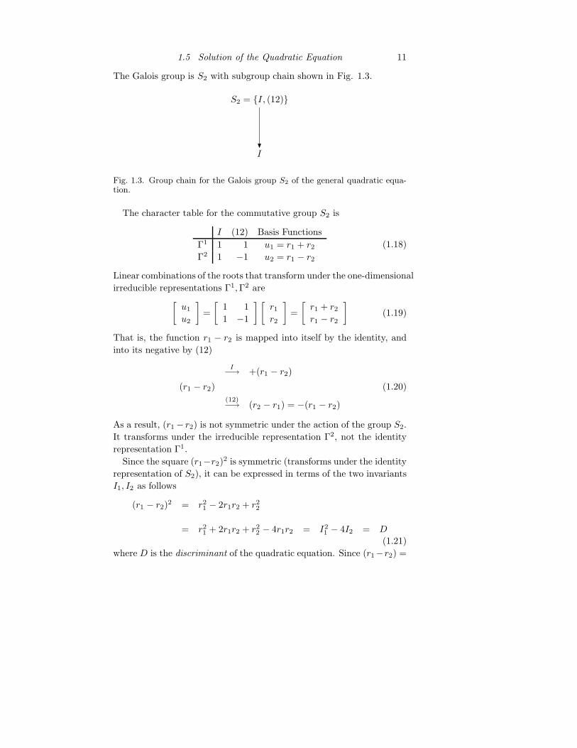
The Galois group is S2 with subgroup chain shown in Fig. 1.3.
S2 = {I, (12)}
I
Fig. 1.3. Group chain for the Galois group S2 of the general quadratic equa-tion.
The character table for the commutative group S2 is
I (12) Basis Functions
Γ1 1 1 u1 = r1 + r2
Γ2 1 −1 u2 = r1 − r2
(1.18)
Linear combinations of the roots that transform under the one-dimensional
irreducible representations Γ1, Γ2 are[
u1
u2
]
=
[
1 1
1 −1
] [
r1
r2
]
=
[
r1 + r2
r1 − r2
]
(1.19)
That is, the function r1 − r2 is mapped into itself by the identity, and
into its negative by (12)
I−→ +(r1 − r2)
(r1 − r2) (1.20)
(12)−→ (r2 − r1) = −(r1 − r2)
As a result, (r1 − r2) is not symmetric under the action of the group S2.
It transforms under the irreducible representation Γ2, not the identity
representation Γ1.
Since the square (r1−r2)2 is symmetric (transforms under the identity
representation of S2), it can be expressed in terms of the two invariants
I1, I2 as follows
(r1 − r2)2 = r2
1 − 2r1r2 + r22
= r21 + 2r1r2 + r2
2 − 4r1r2 = I21 − 4I2 = D
(1.21)
where D is the discriminant of the quadratic equation. Since (r1−r2) =
12 Introduction
±√
D, we have the following linear relation between roots and symmetric
functions:[
1 1
1 −1
] [
r1
r2
]
=
[
I1
±[I21 − 4I2]
1/2
]
(1.22)
Inversion of a square matrix involves a sequence of linear operations.
We find[
r1
r2
]
=1
2
[
1 1
1 −1
] [
I1
±√
D
]
(1.23)
The roots are
r1, r2 =1
2(I1 ±
√D) (1.24)
We solve the quadratic equation by another procedure, which we use
in the following two sections to simplify the cubic and quartic equa-
tions. This method is to move the origin to the mean value of the roots
by defining a new variable, x, in terms of z [c.f., Equ. (1.15)] by a
Tschirnhaus transformation
z = x +1
2I1 (1.25)
The quadratic equation for the new coordinate is
x2 − I ′1x + I ′2 = x2 + I ′2 = 0
I ′1 = 0 (1.26)
I ′2 = I2 −(
1
2I1
)2
The solutions for this auxiliary equation are constructed by radicals
x = ±√
−I ′2 (1.27)
from which we easily construct the roots of the original equation
r1,2 =1
2
(
I1 ±√
I21 − 4I2
)
(1.28)
1.6 Solution of the Cubic Equation
The general cubic equation has the form
(z − s1)(z − s2)(z − s3) = z3 − I1z2 + I2z − I3 = 0

1.6 Solution of the Cubic Equation 13
I1 = s1 + s2 + s3
I2 = s1s2 + s1s3 + s2s3 (1.29)
I3 = s1s2s3
The Galois group is S3 with subgroup chain shown in Fig. 1.4.
S3
A3 S2
I
Fig. 1.4. Group chain for the Galois group S3 of the general cubic equation.
Since A3 is an invariant subgroup of S3 and I is an invariant subgroup
of A3, the first of the two conditions of the Galois theorem (there exists
a chain of invariant subgroups) is satisfied. Since S3/A3 = S2 is com-
mutative and A3/I = A3 is commutative, the second condition is also
satisfied. This means that the general cubic equation can be solved.
We begin the solution with the last group-subgroup pair in this chain:
A3 ⊃ I. The character table for the commutative group A3 is
I (123) (321) Basis Functions
Γ1 1 1 1 v1 = s1 + s2 + s3
Γ2 1 ω ω2 v2 = s1 + ωs2 + ω2s3
Γ3 1 ω2 ω v3 = s1 + ω2s2 + ωs3
(1.30)
where
ω3 = +1, ω = e2πi/3 =−1 + i
√3
2(1.31)
Linear combinations of the roots that transform under each of the three
one-dimensional irreducible representations are easily constructed
v1
v2
v3
=
1 1 1
1 ω ω2
1 ω2 ω
s1
s2
s3
=
s1 + s2 + s3
s1 + ωs2 + ω2s3
s1 + ω2s2 + ωs3
(1.32)
14 Introduction
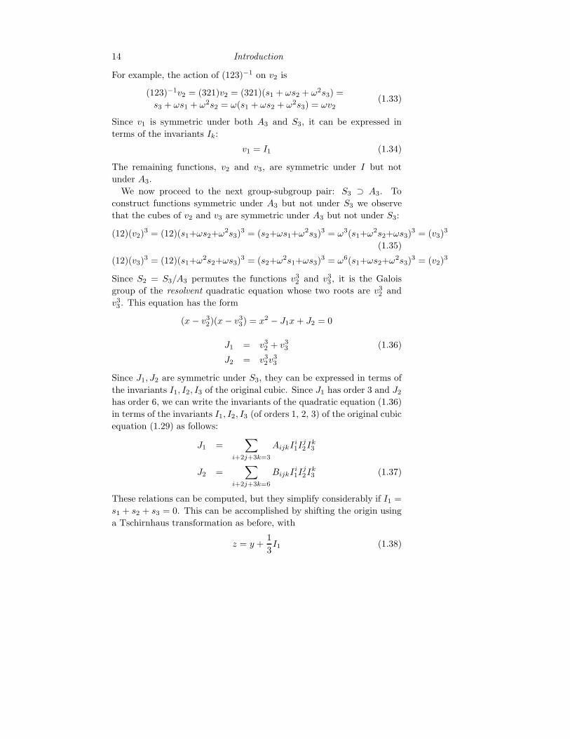
For example, the action of (123)−1 on v2 is
(123)−1v2 = (321)v2 = (321)(s1 + ωs2 + ω2s3) =
s3 + ωs1 + ω2s2 = ω(s1 + ωs2 + ω2s3) = ωv2(1.33)
Since v1 is symmetric under both A3 and S3, it can be expressed in
terms of the invariants Ik:
v1 = I1 (1.34)
The remaining functions, v2 and v3, are symmetric under I but not
under A3.
We now proceed to the next group-subgroup pair: S3 ⊃ A3. To
construct functions symmetric under A3 but not under S3 we observe
that the cubes of v2 and v3 are symmetric under A3 but not under S3:
(12)(v2)3 = (12)(s1+ωs2+ω2s3)
3 = (s2+ωs1+ω2s3)3 = ω3(s1+ω2s2+ωs3)
3 = (v3)3
(1.35)
(12)(v3)3 = (12)(s1+ω2s2+ωs3)
3 = (s2+ω2s1+ωs3)3 = ω6(s1+ωs2+ω2s3)
3 = (v2)3
Since S2 = S3/A3 permutes the functions v32 and v3
3 , it is the Galois
group of the resolvent quadratic equation whose two roots are v32 and
v33 . This equation has the form
(x − v32)(x − v3
3) = x2 − J1x + J2 = 0
J1 = v32 + v3
3 (1.36)
J2 = v32v3
3
Since J1, J2 are symmetric under S3, they can be expressed in terms of
the invariants I1, I2, I3 of the original cubic. Since J1 has order 3 and J2
has order 6, we can write the invariants of the quadratic equation (1.36)
in terms of the invariants I1, I2, I3 (of orders 1, 2, 3) of the original cubic
equation (1.29) as follows:
J1 =∑
i+2j+3k=3
AijkIi1I
j2Ik
3
J2 =∑
i+2j+3k=6
BijkIi1I
j2Ik
3 (1.37)
These relations can be computed, but they simplify considerably if I1 =
s1 + s2 + s3 = 0. This can be accomplished by shifting the origin using
a Tschirnhaus transformation as before, with
z = y +1
3I1 (1.38)
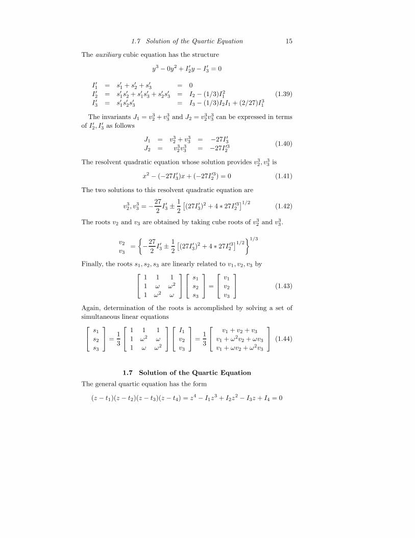
1.7 Solution of the Quartic Equation 15
The auxiliary cubic equation has the structure
y3 − 0y2 + I ′2y − I ′3 = 0
I ′1 = s′1 + s′2 + s′3 = 0
I ′2 = s′1s′
2 + s′1s′
3 + s′2s′
3 = I2 − (1/3)I21
I ′3 = s′1s′
2s′
3 = I3 − (1/3)I2I1 + (2/27)I31
(1.39)
The invariants J1 = v32 + v3
3 and J2 = v32v3
3 can be expressed in terms
of I ′2, I′
3 as follows
J1 = v32 + v3
3 = −27I ′3J2 = v3
2v33 = −27I ′32
(1.40)
The resolvent quadratic equation whose solution provides v32 , v
33 is
x2 − (−27I ′3)x + (−27I ′32 ) = 0 (1.41)
The two solutions to this resolvent quadratic equation are
v32 , v3
3 = −27
2I ′3 ±
1
2
[
(27I ′3)2 + 4 ∗ 27I ′32
]1/2(1.42)
The roots v2 and v3 are obtained by taking cube roots of v32 and v3
3 .
v2
v3=
{
−27
2I ′3 ±
1
2
[
(27I ′3)2 + 4 ∗ 27I ′32
]1/2}1/3
Finally, the roots s1, s2, s3 are linearly related to v1, v2, v3 by
1 1 1
1 ω ω2
1 ω2 ω
s1
s2
s3
=
v1
v2
v3
(1.43)
Again, determination of the roots is accomplished by solving a set of
simultaneous linear equations
s1
s2
s3
=1
3
1 1 1
1 ω2 ω
1 ω ω2
I1
v2
v3
=1
3
v1 + v2 + v3
v1 + ω2v2 + ωv3
v1 + ωv2 + ω2v3
(1.44)
1.7 Solution of the Quartic Equation
The general quartic equation has the form
(z − t1)(z − t2)(z − t3)(z − t4) = z4 − I1z3 + I2z
2 − I3z + I4 = 0

16 Introduction
I1 = t1 + t2 + t3 + t4I2 = t1t2 + t1t3 + t1t4 + t2t3 + t2t4 + t3t4I3 = t1t2t3 + t1t2t4 + t1t3t4 + t2t3t4I4 = t1t2t3t4
(1.45)
For later convenience we will construct the auxiliary quartic by shifting
the origin of coordinates through the Tschirnhaus transformation z =
z′ + 14I1
(z′ − t1)(z′ − t2)(z
′ − t3)(z′ − t4) = z′4 − I ′1z
′3 + I ′2z′2 − I ′3z
′ + I ′4 = 0
I ′1 = 0
I ′2 = I2 − 38I2
1
I ′3 = I3 − 12I2I1 + 1
8I33
I ′4 = I4 − 14I3I1 + 1
16I2I21 − 3
44 I41
(1.46)
S4
V8 A4 S3
V4 A3 S2
I
Fig. 1.5. Group chain for the Galois group S4 of the general quartic equation.
The Galois group is S4. This has the subgroup chain shown in Fig.
1.5. The alternating group A4 consists of the twelve group opera-
tions that have determinant +1 in the permutation matrix represen-
tation. The fourgroup (vierergruppe, Klein group, Klein four-group) V4
is {I, (12)(34), (13)(24), (14), (23)}. The chain
S4 ⊃ A4 ⊃ V4 ⊃ I
satisfies both conditions of Galois’ theorem. In particular
(i) A4 is invariant in S4 and S4/A4 = S2
(ii) V4 is invariant in A4 and A4/V4 = C3 = {I, (234), (432)}
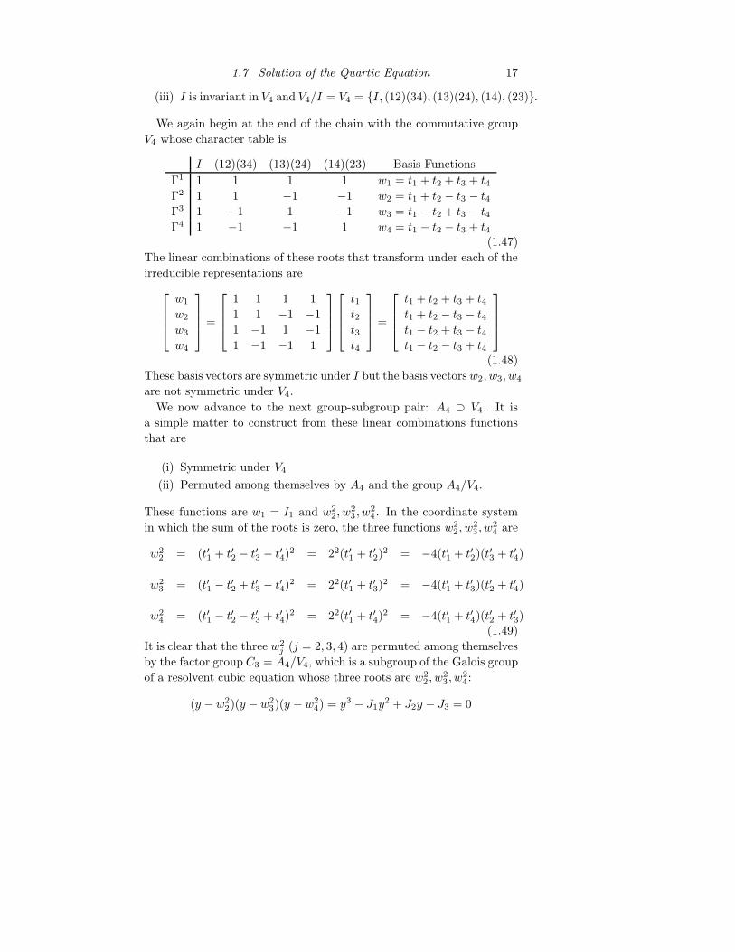
1.7 Solution of the Quartic Equation 17
(iii) I is invariant in V4 and V4/I = V4 = {I, (12)(34), (13)(24), (14), (23)}.
We again begin at the end of the chain with the commutative group
V4 whose character table is
I (12)(34) (13)(24) (14)(23) Basis Functions
Γ1 1 1 1 1 w1 = t1 + t2 + t3 + t4Γ2 1 1 −1 −1 w2 = t1 + t2 − t3 − t4Γ3 1 −1 1 −1 w3 = t1 − t2 + t3 − t4Γ4 1 −1 −1 1 w4 = t1 − t2 − t3 + t4
(1.47)
The linear combinations of these roots that transform under each of the
irreducible representations are
w1
w2
w3
w4
=
1 1 1 1
1 1 −1 −1
1 −1 1 −1
1 −1 −1 1
t1t2t3t4
=
t1 + t2 + t3 + t4t1 + t2 − t3 − t4t1 − t2 + t3 − t4t1 − t2 − t3 + t4
(1.48)
These basis vectors are symmetric under I but the basis vectors w2, w3, w4
are not symmetric under V4.
We now advance to the next group-subgroup pair: A4 ⊃ V4. It is
a simple matter to construct from these linear combinations functions
that are
(i) Symmetric under V4
(ii) Permuted among themselves by A4 and the group A4/V4.
These functions are w1 = I1 and w22, w
23 , w
24 . In the coordinate system
in which the sum of the roots is zero, the three functions w22 , w
23 , w
24 are
w22 = (t′1 + t′2 − t′3 − t′4)
2 = 22(t′1 + t′2)2 = −4(t′1 + t′2)(t
′
3 + t′4)
w23 = (t′1 − t′2 + t′3 − t′4)
2 = 22(t′1 + t′3)2 = −4(t′1 + t′3)(t
′
2 + t′4)
w24 = (t′1 − t′2 − t′3 + t′4)
2 = 22(t′1 + t′4)2 = −4(t′1 + t′4)(t
′
2 + t′3)(1.49)
It is clear that the three w2j (j = 2, 3, 4) are permuted among themselves
by the factor group C3 = A4/V4, which is a subgroup of the Galois group
of a resolvent cubic equation whose three roots are w22 , w
23 , w
24 :
(y − w22)(y − w2
3)(y − w24) = y3 − J1y
2 + J2y − J3 = 0
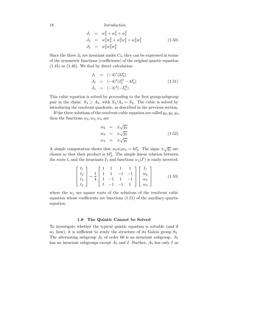
18 Introduction
J1 = w22 + w2
3 + w24
J2 = w22w
23 + w2
2w24 + w2
3w24 (1.50)
J3 = w22w
23w
24
Since the three Jk are invariant under C3, they can be expressed in terms
of the symmetric functions (coefficients) of the original quartic equation
(1.45) or (1.46). We find by direct calculation
J1 = (−4)1(2I ′2)
J2 = (−4)2(I ′22 − 4I ′4) (1.51)
J3 = (−4)3(−I ′23 )
This cubic equation is solved by proceeding to the first group-subgroup
pair in the chain: S4 ⊃ A4, with S4/A4 = S2. The cubic is solved by
introducing the resolvent quadratic, as described in the previous section.
If the three solutions of the resolvent cubic equation are called y2, y3, y4,
then the functions w2, w3, w4 are
w2 = ±√y2
w3 = ±√y3 (1.52)
w4 = ±√y4
A simple computation shows that w2w3w4 = 8I ′3. The signs ±√yj are
chosen so that their product is 8I ′3. The simple linear relation between
the roots ti and the invariants I1 and functions wj(I′) is easily inverted:
t1t2t3t4
=1
4
1 1 1 1
1 1 −1 −1
1 −1 1 −1
1 −1 −1 1
I1
w2
w3
w4
(1.53)
where the wj are square roots of the solutions of the resolvent cubic
equation whose coefficients are functions (1.51) of the auxiliary quartic
equation.
1.8 The Quintic Cannot be Solved
To investigate whether the typical quintic equation is solvable (and if
so, how), it is sufficient to study the structure of its Galois group S5.
The alternating subgroup A5 of order 60 is an invariant subgroup. S5
has no invariant subgroups except A5 and I. Further, A5 has only I as
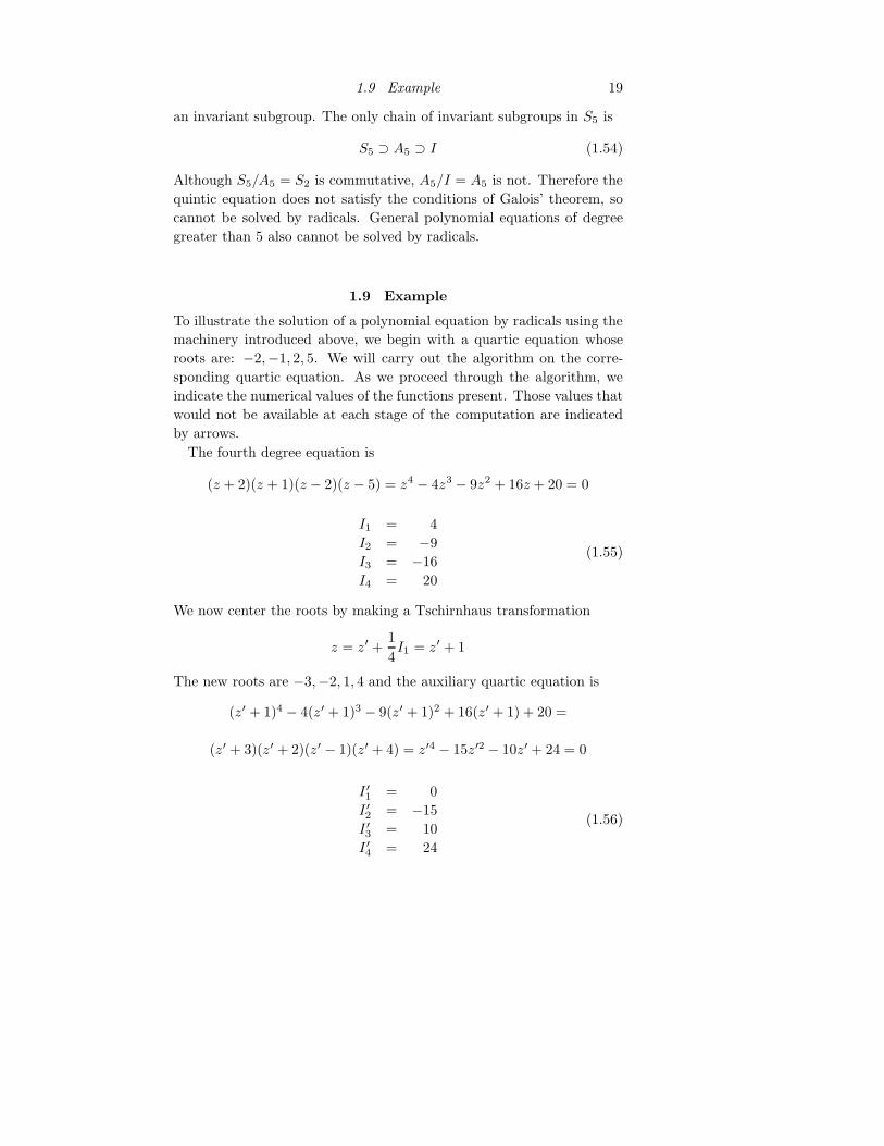
1.9 Example 19
an invariant subgroup. The only chain of invariant subgroups in S5 is
S5 ⊃ A5 ⊃ I (1.54)
Although S5/A5 = S2 is commutative, A5/I = A5 is not. Therefore the
quintic equation does not satisfy the conditions of Galois’ theorem, so
cannot be solved by radicals. General polynomial equations of degree
greater than 5 also cannot be solved by radicals.
1.9 Example
To illustrate the solution of a polynomial equation by radicals using the
machinery introduced above, we begin with a quartic equation whose
roots are: −2,−1, 2, 5. We will carry out the algorithm on the corre-
sponding quartic equation. As we proceed through the algorithm, we
indicate the numerical values of the functions present. Those values that
would not be available at each stage of the computation are indicated
by arrows.
The fourth degree equation is
(z + 2)(z + 1)(z − 2)(z − 5) = z4 − 4z3 − 9z2 + 16z + 20 = 0
I1 = 4
I2 = −9
I3 = −16
I4 = 20
(1.55)
We now center the roots by making a Tschirnhaus transformation
z = z′ +1
4I1 = z′ + 1
The new roots are −3,−2, 1, 4 and the auxiliary quartic equation is
(z′ + 1)4 − 4(z′ + 1)3 − 9(z′ + 1)2 + 16(z′ + 1) + 20 =
(z′ + 3)(z′ + 2)(z′ − 1)(z′ + 4) = z′4 − 15z′2 − 10z′ + 24 = 0
I ′1 = 0
I ′2 = −15
I ′3 = 10
I ′4 = 24
(1.56)

20 Introduction
Next, we introduce linear combinations of the four roots t′1 = −3, t′2 =
−2, t′3 = 1, t′4 = 4
w1
w2
w3
w4
=
1 1 1 1
1 1 −1 −1
1 −1 1 −1
1 −1 −1 1
t′1t′2t′3t′4
→
0
−10
−4
2
(1.57)
Observe at this stage that w2w3w4 = 8I ′3.
Now we compute the squares of these numbers
w22 = y2 → (−10)2 = 100
w23 = y3 → (−4)2 = 16
w24 = y4 → (+2)2 = 4
(1.58)
From the auxiliary quartic (1.56) the resolvent cubic equation can be
constructed
y3 − J1y2 + J2y − J3 = 0
J1 = (−4)1[2I ′2] = (−4)(−30) = 120
J2 = (−4)2[I ′22 − 4I ′4] = 16(225 − 4 ∗ 24) = 2064
J3 = (−4)3[−I ′23 ] = (−64)(−100) = 6400
(1.59)
Note that these are the coefficients of the equation
(y − 22)(y − 42)(y − 102) = y3 − 120y2 + 2064y − 6400 = 0 (1.60)
Now we construct the cubic equation auxiliary to this cubic. This is
done by defining y = y′ + 13J1 = y′ + 1
3 (4 + 16 + 100) = y′ + 40. The
roots are now
y′
1 = y1 − 40 → 4 − 40 = −36
y′
2 = y2 − 40 → 16 − 40 = −24
y′
3 = y3 − 40 → 100 − 40 = 60
(1.61)
The auxiliary cubic is
y′3 − J ′
1y′2 + J ′
2y′ − J ′
3 = 0
J ′
1 = 0
J ′
2 = −2736
J ′
3 = 51840
(1.62)
We note that these are the coefficients of the equation
(y′ + 36)(y′ + 24)(y′ − 60) = 0 (1.63)
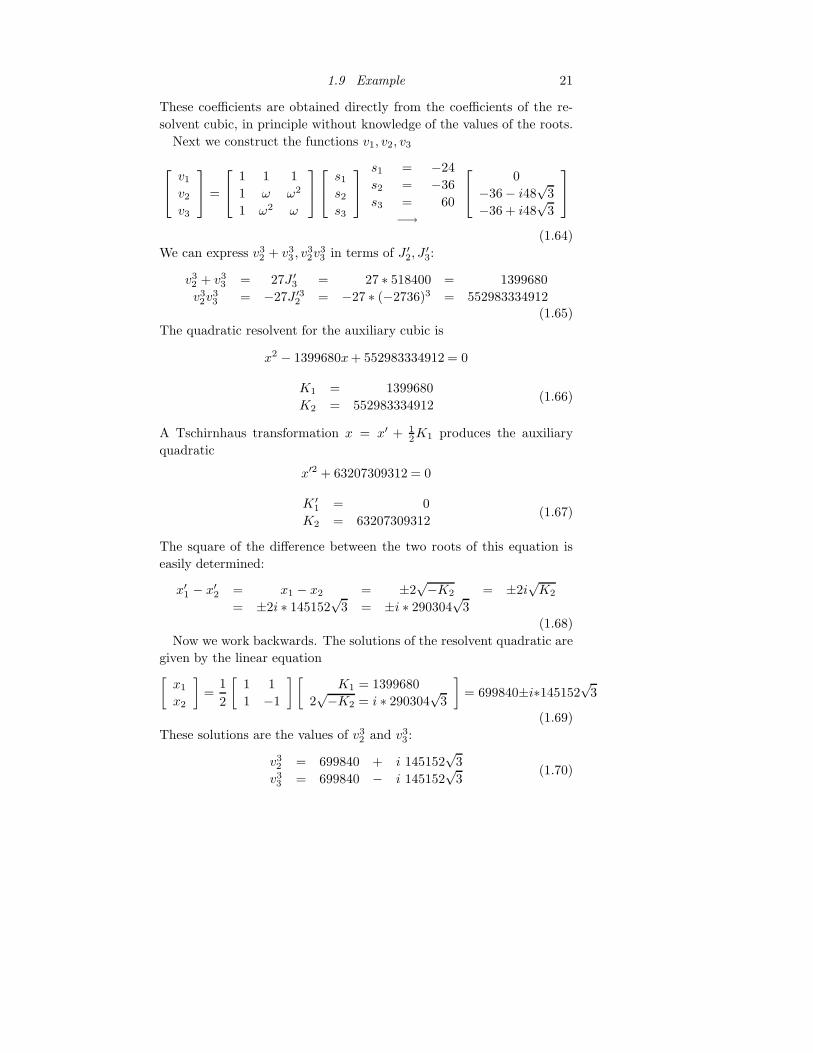
1.9 Example 21
These coefficients are obtained directly from the coefficients of the re-
solvent cubic, in principle without knowledge of the values of the roots.
Next we construct the functions v1, v2, v3
v1
v2
v3
=
1 1 1
1 ω ω2
1 ω2 ω
s1
s2
s3
s1 = −24
s2 = −36
s3 = 60
−→
0
−36 − i48√
3
−36 + i48√
3
(1.64)
We can express v32 + v3
3 , v32v
33 in terms of J ′
2, J′
3:
v32 + v3
3 = 27J ′
3 = 27 ∗ 518400 = 1399680
v32v
33 = −27J ′3
2 = −27 ∗ (−2736)3 = 552983334912(1.65)
The quadratic resolvent for the auxiliary cubic is
x2 − 1399680x + 552983334912 = 0
K1 = 1399680
K2 = 552983334912(1.66)
A Tschirnhaus transformation x = x′ + 12K1 produces the auxiliary
quadratic
x′2 + 63207309312 = 0
K ′
1 = 0
K2 = 63207309312(1.67)
The square of the difference between the two roots of this equation is
easily determined:
x′
1 − x′
2 = x1 − x2 = ±2√−K2 = ±2i
√K2
= ±2i ∗ 145152√
3 = ±i ∗ 290304√
3(1.68)
Now we work backwards. The solutions of the resolvent quadratic are
given by the linear equation[
x1
x2
]
=1
2
[
1 1
1 −1
] [
K1 = 1399680
2√−K2 = i ∗ 290304
√3
]
= 699840±i∗145152√
3
(1.69)
These solutions are the values of v32 and v3
3 :
v32 = 699840 + i 145152
√3
v33 = 699840 − i 145152
√3
(1.70)

22 Introduction
Next, we take cube roots of these quantities. These are unique up to a
factor of ω
v2 = −36 + i48√
3
v3 = −36 − i48√
3(1.71)
The values y1, y2, y3 of the resolvent cubic are complex linear combina-
tions of v2, v3
y1
y2
y3
=1
3
1 1 1
1 ω2 ω
1 ω ω2
J1 = 120
v2 = −36 + i 48√
3
v3 = −36 − i 48√
3
=
16
100
4
(1.72)
w22 = y1 w2 = ±4
w23 = y2 w3 = ±10
w24 = y3 w4 = ±2
(1.73)
Since w2w3w4 = 8I ′3 = 80, an even number of these signs must be neg-
ative. The simplest choice is to take all signs positive. This is different
from the results shown in (1.57); this choice of signs serves only to per-
mute the order of the roots. In the final step, the roots of the original
quartic are linear combinations of w2, w3, w4 and the linear symmetric
function w1 = I1
x1
x2
x3
x4
=1
4
1 1 1 1
1 1 −1 −1
1 −1 1 −1
1 −1 −1 1
I1 = 4
w2 = 4
w3 = 10
w4 = 2
=
20/4 = +5
−4/4 = −1
8/4 = +2
−8/4 = −2
(1.74)
We have recovered the four roots of the original quartic equation using
Galois’ algorithm, based on the structure of the invariance group S4 of
the quartic equation.
1.10 Conclusion
One of the many consequences of Galois’ study of algebraic equations
and the symmetries that leave them invariant is the proof that an al-
gebraic equation can be solved by radicals if and only if its invariance
group has a certain structure. This proof motivated Lie to search for
analogous results involving differential equations and their symmetry
groups, now called Lie groups. We have described in this chapter how
the structure of the discrete symmetry group (Galois group) of a polyno-
mial equation determines whether or not that equation can be solved by

1.11 Problems 23
radicals. If the answer is ‘yes,’ we have shown how the structure of the
Galois group determines the structure of the algorithm for constructing
solutions. This algorithm has been developed for the cubic and quartic
equations, and illustrated by example for a quartic equation.
1.11 Problems
1. Compute S4/A4, A4/V4, V4 and show that they are commutative.
2. Construct the group V8 with the property S4 ⊃ V8 ⊃ V4 (cf. Fig.
1.5). Hint: include a cyclic permutation.
3. For the cubic equation z3 − 7z + 6 = 0 [(z − 1)(z − 2)(z + 3) = 0]
show
I1 = 0 J1 = 162
I2 = −7 J2 = 9261
I3 = −6
Show that the resolvent equation for v32 , v3
3 is (x − v32)(x − v3
3) = x2 −162x + 9261 = 0. Solve this quadratic to find v3
2 , v33 = 81 ± i30
√3, so
that v2, v3 = 12 (3 ± i5
√3). Invert Equ. (1.43) to determine the three
roots of the original equation: (1, 2,−3).
4. Ruler and compass can be used to construct an orthogonal pair
of axes in the plane (Euclid). A compass is used to establish a unit
of length (1). Then by ruler and compass it is possible to construct
intervals of length x, where x is integer. From there it is possible to
construct intervals of lengths x + y, x− y, x ∗ y and x/y using ruler and
compass. It is also possible to construct intervals of length√
x by these
means. The set of all numbers that can be constructed from integers by
addition, subtraction, multiplication, division, and extraction of square
roots is called the set of constructable numbers. This forms a subset of
the numbers x + iy = (x, y) in the complex plane. If a number is (is
not) constructable the point representing that number can (cannot) be
constructed by ruler and compass alone. Since repeated square roots
can be taken, a constructable number satisfies an algebraic equation of
degree K with integer coefficients, where K = 2n must be some power
of two.
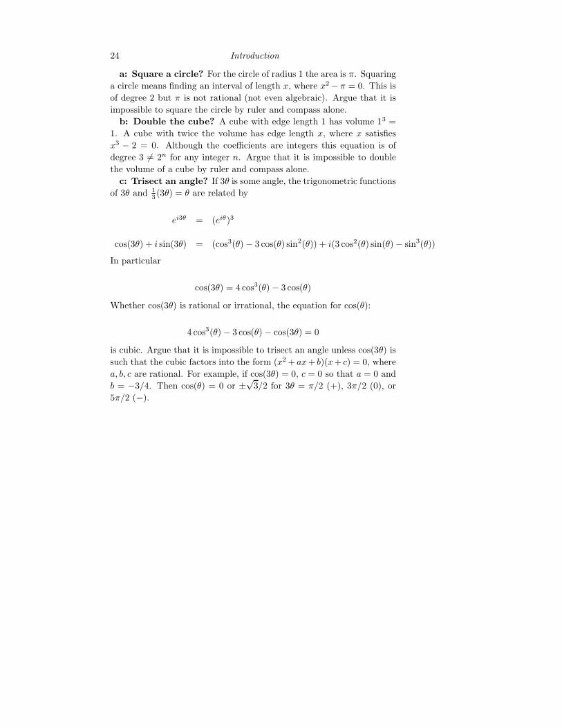
The three geometry problems of antiquity are:
24 Introduction
a: Square a circle? For the circle of radius 1 the area is π. Squaring
a circle means finding an interval of length x, where x2 − π = 0. This is
of degree 2 but π is not rational (not even algebraic). Argue that it is
impossible to square the circle by ruler and compass alone.
b: Double the cube? A cube with edge length 1 has volume 13 =
1. A cube with twice the volume has edge length x, where x satisfies
x3 − 2 = 0. Although the coefficients are integers this equation is of
degree 3 6= 2n for any integer n. Argue that it is impossible to double
the volume of a cube by ruler and compass alone.
c: Trisect an angle? If 3θ is some angle, the trigonometric functions
of 3θ and 13 (3θ) = θ are related by
ei3θ = (eiθ)3
cos(3θ) + i sin(3θ) = (cos3(θ) − 3 cos(θ) sin2(θ)) + i(3 cos2(θ) sin(θ) − sin3(θ))
In particular
cos(3θ) = 4 cos3(θ) − 3 cos(θ)
Whether cos(3θ) is rational or irrational, the equation for cos(θ):
4 cos3(θ) − 3 cos(θ) − cos(3θ) = 0
is cubic. Argue that it is impossible to trisect an angle unless cos(3θ) is
such that the cubic factors into the form (x2 + ax+ b)(x+ c) = 0, where
a, b, c are rational. For example, if cos(3θ) = 0, c = 0 so that a = 0 and
b = −3/4. Then cos(θ) = 0 or ±√
3/2 for 3θ = π/2 (+), 3π/2 (0), or
5π/2 (−).