ent 374 (2007) 156–166www.elsevier.com/locate/scitotenv

Science of the Total Environm

Lidar observations of the diurnal variations in the depthof urban mixing layer: A case study on the air quality

deterioration in Taipei, Taiwan

Charles C.-K. Chou a,⁎, C.-T. Lee b, W.-N. Chen a, S.-Y. Chang a,T.-K. Chen a, C.-Y. Lin a, J.-P. Chen c

a Research Center for Environmental Changes, Academia Sinica, Taipei 115, Taiwan, ROCb Graduate Institute of Environmental Engineering, National Central University, ChungLi 320, Taiwan, ROC

c Department of Atmospheric Sciences, National Taiwan University, Taipei 106, Taiwan, ROC

Received 28 April 2006; received in revised form 1 November 2006; accepted 23 November 2006Available online 31 January 2007

Abstract

An aerosol light detection and ranging (LIDAR) system was used to measure the depth of the atmospheric mixing layer overTaipei, Taiwan in the spring of 2005. This paper presents the variations of the mixing height and the mixing ratios of air pollutantsduring an episode of air quality deterioration (March 7–10, 2005), when Taipei was under an anti-cyclonic outflow of a traveling high-pressure system. It was found that, during those days, the urban mixing height reached its daily maximum of 1.0–1.5 km around noonand declined to 0.3–0.5 km around 18:00 (LST). In terms of hourly averages, the mixing height increased with the ambienttemperature linearly by a slope of 166 m/°C in daytime. The consistency between the changes in the mixing height and in the ambienttemperature implied that the mixing layer dynamics were dominated by solar thermal forcing. As the cap of the mixing layerdescended substantially in the afternoon, reduced dispersion in the shallow mixing layer caused the concentrations of primary airpollutants to increase sharply. Consequently, the pollutant concentration exhibited an anti-correlation with the mixing height. Whileattentions are usually focused on the pollution problems occurring in a morning inversion layer, the results of this study indicatethat the air pollution and its health impacts could be even more severe as the mixing layer is getting shallow in the afternoon.© 2006 Elsevier B.V. All rights reserved.

Keywords: Urban mixing layer; LIDAR; Urban air quality; Tropospheric aerosols

1. Introduction

The mixing layer is the lowest part of the atmospherewhere the constituents of air are mixed due to convectionand mechanical turbulence over the ground (Seibert et al.,

⁎ Corresponding author. Tel.: +886 2 2653 9885; fax: +886 2 27833584.

E-mail address: ckchou@rcec.sinica.edu.tw (C.C.-K. Chou).

0048-9697/$ - see front matter © 2006 Elsevier B.V. All rights reserved.doi:10.1016/j.scitotenv.2006.11.049

2000). Because the emission of air pollutants due tohuman activities are mostly from ground-level sources,mixing layer is usually the most polluted part of theatmosphere, particularly over urban and industrial areas.Considering that the air in the mixing layer is what peopleactually breathe, its composition is therefore of greatpublic concern, and the air quality is generally defined bythe concentrations of air pollutants in the mixing layer.

Given that the dispersion of air pollutants is oftenconfined within the mixing layer, the depth of the

157C.C.-K. Chou et al. / Science of the Total Environment 374 (2007) 156–166

mixing layer, which is usually referred to as the “mixingheight”, is one of the most critical parameters in airquality studies. For decades, there has been a consensusthat the deterioration of air quality is usually caused bythe formation of a shallow mixing layer (e.g., Turner,1969). However, to date, mixing height is not measuredroutinely at most air quality stations. Meteorologicalradiosonde stations may be the only regular data sourcesfor determining this atmospheric structure. Yet theradiosondes are usually launched at 00 and 12 UTConly. Thus, in our time zone (GMT+0800), the sondingmeasurements are made in the morning and earlyevening, respectively, each day. The lack of daytime(particularly mid-day) data prevents us from decipher-ing the diurnal variations of air quality. In recent years,continuous measurements of the mixing height havebeen successfully carried out using the aerosol LIDAR(LIght Detecting And Ranging) technique (e.g., Flamantet al., 1997; Menut et al., 1999; Cohn and Angevine,2000; Chen et al., 2001; Matthias and Bosenberg, 2002;Kunz et al., 2002; Angevine et al., 2003; Mok andRudowicz, 2004). With the advantages of a hightemporal resolution, LIDAR can provide valuable datafor understanding the mixing layer dynamics. Further-more, as the aerosol itself is one of the major airpollutants in an urban atmosphere, the LIDAR signalsare essential for understanding the vertical distributionof air pollutants.

Analyses of the seasonal variations of the airpollutants in Taipei, Taiwan show that their concentra-tions usually reached the maxima in spring. In additionto possible long-range transport from Asian pollutionoutbreaks (e.g., Dibb et al., 2003; Chou et al., 2005),local factors such as a shallow mixing layer may alsocontribute to the high pollution in springtime. In thisstudy, a LIDAR system was used to measure the mixingheight over Taipei Basin, Taiwan during a springpollution episode. The drastic variations of the mixingheight and its implications for the high levels of airpollutants are discussed. Meteorological conditions andmechanism for the development of a shallow mixinglayer in the afternoon are identified. The results indicatethe critical role of the mixing layer dynamics in theformation of a pollution episode.

2. Methods

2.1. Data sources

Data used in this study includes the mass concentra-tions of PM10 and PM2.5 (particulate matter with anaerodynamic diameter of less than 10 and 2.5 μm,

respectively) and light scattering coefficient (at 550 nm)measured at the Taipei (SinJhuang) Supersite. Themixing ratios of gaseous air pollutants (CO, O3, SO2,NOx, Total Hydrocarbons, Non-Methane Hydrocar-bons) measured at the SinJhuang air quality monitoringstation of Taiwan EPA, as well as meteorologicalparameters (barometric pressure, ambient temperature,and surface wind field) measured at the BanChioobservatory of the Central Weather Bureau of Taiwanwere also analyzed. In addition, the vertical profiles ofaerosol in the troposphere, and the depth of the mixinglayer over Taipei were obtained from a ground-basedLIDAR system installed on campus of the NationalTaiwan University. All measurements were assimilatedwith a time resolution of 1 h. These measurement sitesare within 15 km of each other, as shown in the mapgiven in Fig. 1.

2.2. Instrumentation

At the Taipei Supersite, the concentrations of PM10and PM2.5 are measured simultaneously using twoTEOM (Tapered Element Oscillating Microbalance,Model 1400a, Rupprecht and Patashnick Co., Inc.,U.S.A). The light scattering coefficients for 450, 550,and 700 nm are measured by a three-wavelength nephe-lometer (Model 3563, TSI Inc., USA); however, onlythose for 550 nm will be presented in this paper becausethe variations in the scattering coefficients of the othertwo wavelengths were consistent with that of 550 nmin this episode. The sulfate, nitrate, and carbonaceousconstituents in the aerosols are also measured at thesupersite. The results of the aerosol composition will bepresented and discussed in a separate paper.

At the SinJhuang air quality station, which is part ofthe Taiwan Air Quality Monitoring Network (TAQMN)established by the Taiwan EPA in 1993, the mixingratios of SO2, NOx, and O3 are measured using theinstruments manufactured by the Ecotech Inc. (Model9850, 9841, and 9810, respectively), CO is measured bya NDIR-based monitor (Model APMA-360, HORIBALtd., Japan), and those of hydrocarbons are measuredusing a flame ionization detector (Model APHA-360,HORIBA Ltd., Japan).

The LIDAR used in this study is a dual-wavelengthsystem employing the second and third harmonics ofNd-YAG laser at 532 nm and 355 nm with a pulserepetition rate of 20 Hz. The transmitted laser beams aredirected vertically into the atmosphere. A Newtoniantelescope with a diameter of 40 cm is used as thereceiver for the backscattered light. Two narrow bandinterference filters (wavelength center at 355 nm and

Fig. 1. Geographical locations of the observatories in Taipei Basin. (□SJ: SinJhuang air quality station;△S: supersite;●L: lidar observatory;❍BC:BanChiao meteorological station).

158 C.C.-K. Chou et al. / Science of the Total Environment 374 (2007) 156–166

532 nm) with full width at half maximum (FWHM) of0.5 nm are used to reject the background light. Anadditional narrow band filter of 387 nm with an FWHMof 3 nm is employed to measure the Raman signals ofnitrogen at nighttime. The LIDAR was operated 24 heach day to probe the atmosphere, and the signalsreturned from 0.3 to 8 km were analyzed in this work.The raw data resolution of our LIDAR measurement is7.5 m.

2.3. LIDAR data processing and mixing heightdetermination

The signal detected by LIDAR is usually described interms of the range-squared-corrected signal (RSCS),which is defined as

RSCS ¼ P k;zð Þ−PB k;zð Þ½ � � z2 ð1Þ

where P(λ,z) and PB(λ,z) denote the power of thebackscattered light and the background signal from analtitude of z, respectively. The backscattering coefficientof aerosols can be obtained from the inversion of theLIDAR signal following the LIDAR equation:

P k;zð Þ ¼ P0 kð ÞA kð Þz2

bm k;zð Þ þ ba k;zð Þð Þe−2R x

0rm k;zð Þþra k;zð Þ½ �dz

ð2Þ

where P0(λ) is the transmitted power; A(λ) is the systemcalibration factor;σm,a(λ,z) and βm,a(λ,z) denote theextinction and backscattering coefficients of the molec-ular (subscript m) and aerosol (subscript a) constituentsin the atmosphere. For nighttime measurement, thecalculation of βa is based on the Raman inversionalgorithm (Ansmann et al., 1992), whereas the daytimeβa is calculated using a fixed lidar ratio obtained from

159C.C.-K. Chou et al. / Science of the Total Environment 374 (2007) 156–166

the Raman measurements of the previous night (Klett,1981). Lidar ratio depends strongly on the aerosolcomposition as well as the size distribution. Neverthe-less, in this study, the measured lidar ratios (355 nm) foraerosols within boundary layer were mostly ranged from30 sr to 50 sr, and the standard deviation of the lidar ratiofor one night usually less than 10 sr. Thus, in case thenighttime Raman measurement is also not available, afixed lidar ratio of 40 sr would be applied.

Given that the aerosol concentration in the mixinglayer is significantly higher than in the free troposphere,the cap of the mixing layer is characterized by a steepgradient of the aerosol backscattering signal. Flamantet al. (1997) proposed that the altitude of the top of themixing layer could be obtained from the profile of thederivative of the LIDAR signal (i.e. RSCS). In apreliminary study, we have validated the mixing heightmeasurement of our LIDAR system by comparing withthat determined using radiosondes (Chen et al., 2006).Accordingly, in this study, the mixing height is definedat the altitude with the minimum of the first derivative ofRSCS (i.e. dPz2/dz). With this definition, the mixingheight cannot be determined in the case of a stableatmosphere where a very shallow inversion layer couldexist. Given the 300 m altitude gate of our LIDAR, we'llonly report that the mixing height was less than 0.3 kmfor those cases.

3. Results and discussion

3.1. Meteorological conditions

Fig. 2 shows the evolution of the synoptic weathersystems over East Asia, and indicates that a strongtraveling high-pressure system moved along the 30°Nlatitude line, from the Southeast China into the WestPacific Ocean during the period of March 6–10, 2005.Fig. 3(a) illustrates that the barometric pressure (BP) atTaipei reached a high level of 1030 hPa in the earlymorning of March 6, indicating that Taipei was ratherclose to the high center. As the high-pressure systemwas moving away, leaving Taipei under its anti-cyclonicsubsidence, the BP gradually decreased and during thattime the ambient temperature (AT) varied with typicaldiurnal cycles until the next cold front arrived in theearly morning of March 11. The variations of the surface

Fig. 2. Surface weather maps for 0000Z of (a) March 6; (b) March 7; (c)March 10, 2005.A traveling high-pressure systemwasmoving along 30°N from the East China into the West Pacific Ocean. Taipei was on theleeward side of its anti-cyclonic outflow during March 7–10. (Source:Japan Meteorological Agency).

Fig. 3. Hourly variations of (a) barometric pressure, ambienttemperature, and (b) surface winds during the episode of this study.

160 C.C.-K. Chou et al. / Science of the Total Environment 374 (2007) 156–166

winds are shown in Fig. 3(b): When the high-pressuresystem was passing through Taipei, there were firststrong easterlies caused by the steep pressure gradient atthe edge of the high-pressure air mass. The followingdays (March 7–10) were characterized by weaksynoptic winds. Under this setting, moderate sea breezes(2–3 m/s) developed each afternoon as a result of theland-heating effects. It is worth noting that the windspeed decreased drastically while the ambient temper-ature declined, and that the sea-breeze peaks in Fig. 3(b)are exactly coincidental with those of the ambienttemperature shown in Fig. 3(a). The synchronizationbetween the ambient temperature and the wind speedimplies that thermo-forcing was dominant in theboundary layer dynamics in those days, when Taipeiwas on the leeward side of the high mountains(∼2000 m) located on the southeastern rim of the basin.

3.2. Variations in mixing height

The height of the mixing layer was obtained from theprofile of the backscattering signals measured by theLIDAR system. To demonstrate the typical diurnalvariation of the mixing layer, Fig. 4(a)–(b) shows the

time–altitude evolution of the Lidar signal (RSCS) andits first derivative, respectively, for March 7, 2005. Theboundaries between the mixing layer and the freetroposphere were distinctly characterized by the sharpgradient of the aerosol signals. In the morning, most ofthe aerosols were confined within the surface-basedinversion layer. The aerosol layer at 0.8–1 km is mostlikely remnants of the convectively elevated mixinglayer from the previous day. The inversion started tobreak up at about 09:00 (Local Time) and the mixinglayer was thickening. The LIDAR signals clearly showthe evolution of the atmospheric boundary layer,transforming from a stratified to a well-mixed structurein the morning toward the noon. The mixing heightreached a maximum of 1460 m AGL at noon. Fig. 4(b)and (c) illustrates the evolution in the vertical profile ofthe Lidar signal (532 nm). Note that, as shown by theprofiles for 12:00 and 14:00 LST, the aerosol backscat-tering ratio was consistent in the lowest part of theatmosphere, indicating the existence of a well-mixedboundary layer. In this case the boundary layer agreeswith the mixing layer essentially. However, from thederivative of the LIDAR signals shown in Fig. 4(b), wefound that a “sandwich” structure was developed in thelower troposphere in the late afternoon. While the stronginversion between the free troposphere and the bound-ary layer was still there, the vertical mixing had declinedsubstantially and cannot support a mixing layer as highas that at the noontime. As a result, the boundary layerwas divided into two parts: the lower part was themixing layer where the convection was still predomi-nant; the upper part was known as the residual layer thatcontained the aerosols lifted up in the noontimeboundary layer. Fig. 5 shows the temperature profilesretrieved from the radiosonde measurements made at08:00 and 20:00 (LST), respectively, on March 7. Theformation of the surface-based inversion layers shouldhave inhibited the convective mixing, and the mixingheight cannot be defined in this context. One can alsosee the inversion at 1.0–1.2 km in the evening profile,which is corresponding to the boundary between theresidual layer and the free troposphere observed by theLIDAR. The evolution of the boundary layer observedin our study agrees generally with those documented inthe literature (e.g., Stull, 1988; Cohn and Angevine,2000). This consistency warrants a further analysis ofthe boundary layer dynamics based on the LIDARmeasurements.

It is worth noting that the mixing height decreaseddrastically in the afternoon, implying that the develop-ment of the nocturnal boundary layer could have startedseveral hours prior to sunset. Consequently, a substantial

Fig. 4. Evolution of Lidar measurements on March 7, 2005. (a) range-squared-corrected signal; (b) first derivative of the LIDAR signal; (c) verticalprofiles of the backscattering coefficient measured at 9:00, 12:00, 14:00, 16:00, and 18:00 (LST). The offset of each profile was shifted forpresentation. Figures (a) and (b) present 15-min averages of the LIDAR measurements and have a resolution of 7.5 m in altitude.

161C.C.-K. Chou et al. / Science of the Total Environment 374 (2007) 156–166

amount of air pollutants could have been stored in theresidual layer and negatively influencing the air qualityin the downwind area as the mixing layer developed inthe next morning. Such a drastic decrease of the mixingheight in the afternoon is similar to that observed by

Strawbridge and Snyder (2004) in British Columbia,Canada, and the simulation for a case in Barcelona,Spain (Pino et al., 2004). Grimsdell and Angevine(2002) identified two types of afternoon transition of theboundary layer: inversion layer separation (ILS) and

Fig. 5. Radiosonding profiles of (a) temperature and (b) relative humidity in Taipei on March 7, 2005.

162 C.C.-K. Chou et al. / Science of the Total Environment 374 (2007) 156–166

descent. Both types were also observed in our study:Fig. 4 displays a typical ILS transition pattern, and Fig. 6shows the case of descent transition occurred on March

Fig. 6. Time–height plots of (a) range-squared-corrected signal and (b) the ffigures present 15-min averages of the LIDAR measurements and have a re

10. They also noticed that the transition sometimes startsin the very early afternoon, similar to the results reportedin this paper.

irst derivative of the LIDAR signal measured on March 10, 2005. Thesolution of 7.5 m in altitude.

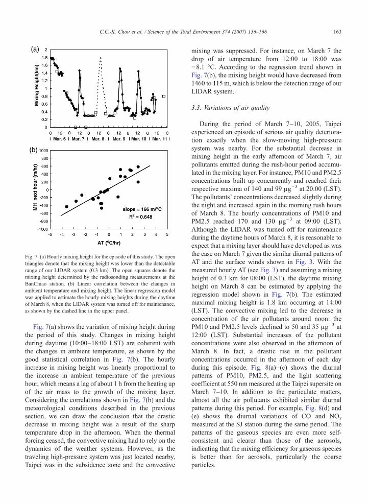
Fig. 7. (a) Hourly mixing height for the episode of this study. The opentriangles denote that the mixing height was lower than the detectablerange of our LIDAR system (0.3 km). The open squares denote themixing height determined by the radiosonding measurements at theBanChiao station. (b) Linear correlation between the changes inambient temperature and mixing height. The linear regression modelwas applied to estimate the hourly mixing heights during the daytimeof March 8, when the LIDAR system was turned off for maintenance,as shown by the dashed line in the upper panel.

163C.C.-K. Chou et al. / Science of the Total Environment 374 (2007) 156–166

Fig. 7(a) shows the variation of mixing height duringthe period of this study. Changes in mixing heightduring daytime (10:00–18:00 LST) are coherent withthe changes in ambient temperature, as shown by thegood statistical correlation in Fig. 7(b). The hourlyincrease in mixing height was linearly proportional tothe increase in ambient temperature of the previoushour, which means a lag of about 1 h from the heating upof the air mass to the growth of the mixing layer.Considering the correlations shown in Fig. 7(b) and themeteorological conditions described in the previoussection, we can draw the conclusion that the drasticdecrease in mixing height was a result of the sharptemperature drop in the afternoon. When the thermalforcing ceased, the convective mixing had to rely on thedynamics of the weather systems. However, as thetraveling high-pressure system was just located nearby,Taipei was in the subsidence zone and the convective

mixing was suppressed. For instance, on March 7 thedrop of air temperature from 12:00 to 18:00 was−8.1 °C. According to the regression trend shown inFig. 7(b), the mixing height would have decreased from1460 to 115 m, which is below the detection range of ourLIDAR system.

3.3. Variations of air quality

During the period of March 7–10, 2005, Taipeiexperienced an episode of serious air quality deteriora-tion exactly when the slow-moving high-pressuresystem was nearby. For the substantial decrease inmixing height in the early afternoon of March 7, airpollutants emitted during the rush-hour period accumu-lated in the mixing layer. For instance, PM10 and PM2.5concentrations built up concurrently and reached theirrespective maxima of 140 and 99 μg–3 at 20:00 (LST).The pollutants’ concentrations decreased slightly duringthe night and increased again in the morning rush hoursof March 8. The hourly concentrations of PM10 andPM2.5 reached 170 and 130 μg–3 at 09:00 (LST).Although the LIDAR was turned off for maintenanceduring the daytime hours of March 8, it is reasonable toexpect that a mixing layer should have developed as wasthe case on March 7 given the similar diurnal patterns ofAT and the surface winds shown in Fig. 3. With themeasured hourly AT (see Fig. 3) and assuming a mixingheight of 0.3 km for 08:00 (LST), the daytime mixingheight on March 8 can be estimated by applying theregression model shown in Fig. 7(b). The estimatedmaximal mixing height is 1.8 km occurring at 14:00(LST). The convective mixing led to the decrease inconcentration of the air pollutants around noon: thePM10 and PM2.5 levels declined to 50 and 35 μg–3 at12:00 (LST). Substantial increases of the pollutantconcentrations were also observed in the afternoon ofMarch 8. In fact, a drastic rise in the pollutantconcentrations occurred in the afternoon of each dayduring this episode. Fig. 8(a)–(c) shows the diurnalpatterns of PM10, PM2.5, and the light scatteringcoefficient at 550 nmmeasured at the Taipei supersite onMarch 7–10. In addition to the particulate matters,almost all the air pollutants exhibited similar diurnalpatterns during this period. For example, Fig. 8(d) and(e) shows the diurnal variations of CO and NOx

measured at the SJ station during the same period. Thepatterns of the gaseous species are even more self-consistent and clearer than those of the aerosols,indicating that the mixing efficiency for gaseous speciesis better than for aerosols, particularly the coarseparticles.

164 C.C.-K. Chou et al. / Science of the Total Environment 374 (2007) 156–166

In addition to the decreased mixing height, the drasticincreases of the ground-level concentrations of airpollutants in the afternoon can also be attributed to otherfactors. One of the possible reasons is a shift in winddirection; however, our results suggest that the influencedue to wind direction was relatively minor in the episodeof this study. Fig. 3(b) shows that there was indeed adiurnal cycle of wind direction during the episode.However, the shift in wind direction usually occurred ataround 19:00–20:00 LST, several hours after the pollutantconcentration started to increase (see Fig. 8). Increases inemissions can certainly result in the observed phenomena.In fact, it is difficult to precisely separate the effect of

Fig. 8. Diurnal patterns of the concentrations of air pollutants and light sca550 nm; (d) CO; (e) NOx; (f) O3.

afternoon rush hours from that of a shrinkingmixing layer.One reasonable approach is to compare the diurnal patternof a pollutant for a specific episode with that for averageconditions. Fig. 9(a)–(b) illustrates such a comparison oftwo typical transportation pollutants, CO and NOx: theaverages for the episode are comparedwith their respectivemonthly averages. One can see that the increases in theambient levels of air pollutants during rush hours are muchmore pronounced in this episode than under averageconditions. The evening peaks of both CO and NOx of theepisode are higher than their respective monthly averagesby a factor of about two, indicating the strong influencesdue to factors other than rush-hour emissions.

ttering coefficient. (a) PM10; (b) PM2.5; (c) scattering coefficient for

Table 1The correlation coefficients between the mixing height and theambient concentrations of the respective air pollutants in the afternoon(13:00–18:00) of each day

March 7 March 9 March 10

PM10 −0.0048 −0.7460 −0.9690PM2.5 −0.2105 −0.7240 −0.9901bscat_550 nm 0.1831 −0.7368 −0.9643CO −0.7045 −0.9268 −0.8200NOx −0.6280 −0.8407 −0.9429NMHC −0.7111 −0.8724 −0.9225THC −0.8095 −0.8286 −0.9440O3 0.6929 0.5052 0.9588SO2 0.4139 −0.8432 0.0088

165C.C.-K. Chou et al. / Science of the Total Environment 374 (2007) 156–166

Table 1 summarizes the linear correlation coefficientsbetween the mixing height and the ambient concentra-tion of each air pollutant for the time periods of 13:00–18:00 of March 7 and March 9–10, respectively. OnMarch 7, prior to the episode, the correlation wasrelatively weak. In contrast, on March 10, almost perfectanti-correlations between the mixing height and thepollutant concentrations were found. The concentrationsof air pollutants and the light scattering by aerosolsincreased proportionally when the mixing heightdecreased in the afternoon. This shows that the airpollutants were concentrated when the cap of the mixinglayer was descending. The poor correlation between SO2

and mixing height is not clear yet. Nevertheless, theresults show that the concentration of SO2 in Taipei basinwas dominated by factors other than the convectivemixing. The concentration of ozone was positivelycorrelated with the mixing height. In Fig. 8(f) the diurnalcycle of ozone mixing ratio indicates that photochemicalreactions prevailed during daytime of the episode. Thus,it is reasonable to infer that there was a substantialamount of secondary pollutants formed through photo-

Fig. 9. Comparison between the diurnal variations of typicaltransportation pollutants (CO and NOx) for the episode (March 7–10)and the monthly average of March 2005. The error bars are for thestandard deviations of the average values.

chemical reactions within the mixing layer. Theformation of secondary aerosols may explain why theparticulate measurements (PM10, PM2.5, and lightscattering coefficient) did not significantly decrease asdid the gaseous species around noontime due toconvective dispersion (Fig. 8). The secondary aerosolswere accumulated in the mixing layer, and wereconcentrated in the afternoon, when the mixing heightwas decreased. The daily-based anti-correlation betweenthe aerosol measurements and the mixing heightwarrants that the ambient concentration of aerosols wasdominated by the mixing layer dynamics. The extent ofphotochemical reactions should also be important to theambient level of aerosols; however, a conclusive remarkfor the interactions between meteorological and photo-chemical effects cannot be drawn in this context.

Another noteworthy feature is the built up ofnighttime pollutant concentrations as shown in Fig. 8.It is suggested that the daily build up of pollutants in thenight could be a result of the weakening winds (shownin Fig. 3(b)). Evidently wind advection played a criticalrole in the nighttime air quality, whereas the convectivemixing predominated in the daytime. In the case wherethe synoptic weather conditions tended to inhibitadvection, a stagnant atmosphere was formed, resultingin the accumulation of air pollutants during the night.

4. Conclusions

The variation of urban mixing layer and itsimplication for the air quality deterioration episode inTaipei, Taiwan was studied with air quality monitoringdata and LIDAR measurements. We found that theurban mixing heights grow proportional to the changesin ambient air temperature with a lag of 1 h. The cap ofthe mixing layer descended drastically as the thermalforcing declined in the afternoon during this springtimeepisode. In addition, the shallow mixing layer in the

166 C.C.-K. Chou et al. / Science of the Total Environment 374 (2007) 156–166

afternoon was also attributed partly to the anti-cyclonicsubsidence of a nearby high-pressure system. Synopticconditions inhibited advection and convection of theboundary layer air mass, and therefore reduced themechanical forcing for the mixing layer.

During the episode examined in this study, theambient levels of the air pollutants, except ozone,increased consistently with the decreases in mixingheight in the afternoon, indicating that the high mixingratios of the air pollutants in the evening resulted from areduced dispersion volume. The mixing ratio of ozone, atypical secondary pollutant due to the photochemistry inthe troposphere, exhibited a positive correlation with themixing height. The positive correlation was a result oftheir common forcing, i.e. solar irradiation. Inferred fromthis is a substantial production of secondary aerosols,which later on accumulated and resulted in highconcentrations of particulate matters in the evening.

The influence of convective mixing on the air qualityhas been recognized for decades, yet data showing thisphenomenon remain rather limited for the lack oftemporal resolution in the mixing height measurement.The development and application of LIDAR have madesuch an investigation possible. Besides, to date, moreattention is usually focused on the pollution problemsoccurring in a morning inversion layer. The results ofthis study indicated that the air pollution could be evenmore severe while the mixing layer is getting shallow inthe afternoon. Considering the fact that an improvementin the understanding of boundary layer dynamics willmost certainly contribute to the development of an airquality forecast model, a well-designed long-term studycombining LIDAR and atmospheric chemistry measure-ments is urgently needed.

Acknowledgements

This work was supported by the Nation ScienceCouncil of Taiwan, R.O.C. through grants NSC-90–2119-M-002–013, NSC-94-EPA-Z-008–003, NSC-94–2111-M-001–004, and NSC-95–2111-M-001–004. Par-tial funding support for the lidar instrument from theCollege of Science, National Taiwan University, is alsogreatly appreciated.

References

Angevine WM, White AB, Senff CJ, Trainer M, Banta RM, AyoubMA. Urban–rural contrasts in mixing height and cloudiness overNashville in 1999. J Geophys Res 2003;108:4092.

Ansmann A, Wandinger U, Riebesell M, Weitkamp C, Michaelis W.Independent measurement of extinction and backscatter profiles incirrus clouds by using a combined Raman elastic-backscatter lidar.Appl Opt 1992;31:7113–31.

Chen W, Kuze H, Uchiyama A, Suzuki Y, Takeuchi N. One-yearobservation of urban mixed layer characteristics at Tsukuba, Japanusing a micro pulse lidar. Atmos Environ 2001;35:4273–80.

Chen WN, Lin PH, Chen TK, Chou CCK, Chen JP. Diurnal cycle ofmixing measured by lidar. 23rd International Laser RadarConference, Nara, Japan, July 24–28; 2006.

Chou CCK, Huang SH, Chen TK, Lin CY, Wang LC. Size-segregatedcharacterization of atmospheric aerosols in Taipei during Asianoutflow episodes. Atmos Res 2005;75:89-109.

Cohn SA, Angevine WM. Boundary layer height and entrainmentzone thickness measured by lidars and wind profiling radars.J Appl Meterol 2000;39:1233–47.

Dibb JE, Talbot RW, Scheuer EM, Seid G, Avery MA, Singh H.Aerosol chemical composition in Asian continental outflow duringthe TRACE-P campaign: comparison with PEM-West B. J Geo-phys Res 2003;108:8815.

Flamant C, Pelon J, Flamant PH, Durand P. Lidar determination of theentrainment zone thickness at the top of the unstable marineatmospheric boundary-layer. Boundary - Layer Meteorol 1997;83:247–84.

Grimsdell AW, Angevine WM. Observations of the afternoontransition of the convective boundary layer. J Appl Meteorol2002;41:3.

Klett JD. Stable analytical inversion solution for processing lidarreturns. Appl Opt 1981;20:211–20.

Kunz GJ, Leeuw G, Becker E, O'Dowd CD. Lidar observations ofatmospheric boundary layer structure and sea spray aerosol plumesgeneration and transport at Mace Head, Ireland (PARFORCEexperiment). J Geophys Res 2002;107:8106.

Matthias V, Bosenberg J. Aerosol climatology for the planetaryboundary layer derived from regular lidar measurements. AtmosRes 2002;63:221–45.

Menut L, Flamant C, Pelon J, Flamant PH. Urban boundary-layerheight determination from lidar measurements over the Paris area.Appl Opt 1999;38:945–54.

Mok TM, Rudowicz CZ. A lidar study of the atmospheric entrainmentzone and mixed layer over Hong Kong. Atmos Res 2004;69:147–63.

Pino D, Vila-Guerau de Arellano J, Comeron A, Rocadenbosch F. Theboundary layer growth in an urban area. Sci Total Environ2004;334–335:207–13.

Seibert P, Beyrich F, Gryning SE, Joffre S, Rasmussen A, Tercier P.Review and intercomparison of operational methods for thedetermination of the mixing height. Atmos Environ 2000;34:1001–27.

Strawbridge KB, Snyder BJ. Planetary boundary layer heightdetermination during Pacific 2001 using the advantage of ascanning lidar instrument. Atmos Environ 2004;38:5861–71.

Stull RB. An introduction to boundary layer meteorology. Nether-lands: Kluwer Academic Publishers; 1988.

Turner DB. Workbook of atmospheric diffusion estimates. U.S. EPAReport 999-AP-26, Washington, D.C.; 1969.