LIDAR and Vision-Based Pedestrian Detection System - …home.isr.uc.pt/~cpremebida/files_cp/LIDAR...

• • • • • • • • • • • • • • • • • • • • • • • • • • • • • • •

LIDAR and Vision-BasedPedestrian Detection System

Cristiano Premebida, Oswaldo Ludwig,and Urbano NunesInstitute for Systems and RoboticsDepartment of Electrical and ComputerEngineeringUniversity of CoimbraCoimbra 3030-290, Portugale-mail: [email protected],[email protected], [email protected]

Received 11 September 2008; accepted 30 July 2009

A perception system for pedestrian detection in urban scenarios using information froma LIDAR and a single camera is presented. Two sensor fusion architectures are described,a centralized and a decentralized one. In the former, the fusion process occurs at the fea-ture level, i.e., features from LIDAR and vision spaces are combined in a single vectorfor posterior classification using a single classifier. In the latter, two classifiers are em-ployed, one per sensor-feature space, which were offline selected based on informationtheory and fused by a trainable fusion method applied over the likelihoods providedby the component classifiers. The proposed schemes for sensor combination, and morespecifically the trainable fusion method, lead to enhanced detection performance and, inaddition, maintenance of false-alarms under tolerable values in comparison with single-based classifiers. Experimental results highlight the performance and effectiveness of theproposed pedestrian detection system and the related sensor data combination strategies.C© 2009 Wiley Periodicals, Inc.

1. INTRODUCTION

Intelligent ground vehicles as well as mobile robots,navigating in environments with static and dynamicobjects around, e.g., other vehicles, mobile robots,and vulnerable road users (particularly pedestrians),should be provided with perception systems whoseprimary function is to detect and classify surround-ing objects, having in view to avoid collisions and tomitigate situations of risk during the navigation. Akey element of a perception system can be a singleand reasonable cost-affordable sensor or, on the otherhand, a set of multiple sensors for providing data

to higher decision levels in charge of performingclassification and/or situation assessment. Thecomplementary and redundant information that canbe obtained using a multisensor architecture shouldbe properly explored to maximize the inferenceand confidence levels in object detection, whichconstitute a prerequisite for a complete pedestrianprotection system.

The integration of a LIDAR (LIght Detection AndRanging) sensor and a camera, to bring redundancyand complementary characteristics for improvingthe detection system’s reliability and accuracy, hadgained the attention of the intelligent vehicles (IV)

Journal of Field Robotics 26(9), 696–711 (2009) C© 2009 Wiley Periodicals, Inc.Published online in Wiley InterScience (www.interscience.wiley.com). • DOI: 10.1002/rob.20312

Premebida et al.: LIDAR and Vision-Based Pedestrian Detection System • 697

SegmentationSegments: Sk

CoordinateTransformation

LIDARfeatures Classifier_LIDAR

Vision features(HOG/COV) Classifier

Fusionscheme

Likelihoodp(X(k)|q)

Likelihoodp(X(k)|q)

ROIFeature

Combination

Classifier_Vision

Preprocessing module Feature extraction Fusion module

Decentralized scheme

Centralized scheme

Figure 1. Sensor fusion architecture composed of three modules: preprocessing, feature extraction, and fusion.

and mobile robotics research communities in the pastfew years. Handling this multisensorial problem isnot just a matter of determining regions of interest(ROI) in the image to perform vision-based classifica-tion; in fact, many important steps have to be prop-erly addressed before a high-level combination canbe achieved. This work attempts to contribute to thesolution of the pedestrian detection problem usingan ensemble of classifiers fusing LIDAR and visiondata.

This paper presents research results on central-ized and decentralized schemes proposed to com-bine range and visual information, gathered by aIbeo Alasca-XT LIDAR and an Allied Guppy camerasetup, mounted in an electrical vehicle (detailed inSection 2), with the main goal of performing pedes-trian detection in outdoor urban-like scenarios. Theproposed system is composed of three main modules:preprocessing, feature extraction, and fusion mod-ules (see Figure 1).

The preprocessing module, presented inSection 2, is in charge of data acquisition, segmen-tation (in the laser space), and ROI determinationin the image plane. Basically, this module generatesthe entities/objects of interest for further classifi-cation. The feature extraction module, detailed inSection 3, calculates two categories of features: a15-dimensional laser-based feature vector and theimage-based feature array composed of histogramof oriented gradients (HOG) and covariance (COV)features. The fusion module involves the classifica-tion methods, described in Section 4, and the fusionarchitectures: centralized and decentralized. In the

former, the best classifier, applied over the wholefeature space, is used to perform the final inference,whereas in the latter the likelihoods provided bytwo classifiers, one per feature space, are combinedthrough a set of fusion methods; the pair of classifierswas selected based on a maximum relevance andminimal redundancy criterion (mRMR) (Peng, Long,& Ding, 2005). Finally, the fusion schemes, catego-rized as trainable fusion methods and nontrainablefusion rules, are outlined in Section 5.

The proposed fusion schemes for pedestrian de-tection were validated using our data set, which waspreviously separated in training and testing parts,each part corresponding to different conditions underwhich the data were collected. Experimental resultsare reported and analyzed in Section 6, with empha-sis on the results obtained with the proposed train-able fusion methods. Finally, conclusions are drawnin Section 7.

Table I surveys some significant related workson pedestrian detection using LIDAR and monocu-lar visible-spectrum cameras. Other relevant relatedworks are Gandhi and Trivedi (2007) on pedestrianprotection systems and Hall and Llinas (1997) onmultisensor data fusion.

This paper makes some contributions withinthe pedestrian detection theme, which are mainlythreefold:

1. LIDAR-based classifiers: A set of consistentmethods is used to classify pedestrians usinga feature vector with 15 components, some ofthem proposed in this work.

Journal of Field Robotics DOI 10.1002/rob

698 • Journal of Field Robotics—2009

Table I. Survey of some related work on vision and LIDAR–based perception systems for pedestrian and on-road objectdetection/classification in outdoor scenarios.

Ref. Vision system LIDAR system Comments

Douillard et al.,2007

Monocular colorcamera. Conditionalrandom fields(CRFs) trained withvirtual evidenceboosting (VEB).

Single-layer LIDAR.Geometrical information isprocessed from the LIDARdata to estimate/classifythe objects as vehicles ornonvehicles.

To deal with the problem of object scalevariations in the images, the rangeinformation provided by the LIDAR isused during the CRF classification. Theclassification method was evaluated andcompared in several features:geometrical (from laser data), visual(color and texture), and combination ofboth. The CRF and a LogitBoost classifierwere also compared.

Spinello andSiegwart,2008

HOG–SVM classifierbased on monocularcolor images.

A multilayer LIDAR (IbeoAlasca XT) is employed todetect on-road objectswhose positions areprojected into the imageplane.

The object’s position is detected by theLIDAR, and the vision-based systemclassifies the detected objects aspedestrian or nonpedestrian. A Bayesiandecomposed expression is used as thereasoning fusion rule.

Pangop,Chapuis,Bonnet,Cornou, andChausse, 2008

An Adaboost classifier,trained withHaar-like features, isused to classifypedestrians.

An Ibeo Alasca XT LIDAR isemployed for objectsegmentation, tracking,and detection.

The speed, estimated during the trackingprocess, and the vision score–basedlikelihood are fused in a Bayesianframework using an autoregressive (AR)formalism to model the observations.

Hwang, Cho,Ryu, Park,and Kim,2007

Monocular colorcamera. Amultiple-SVMclassifier is used toverify the hypothesiscandidates inside theROIs.

Single-layer LIDAR. Theentities detected by theLIDAR generate hypothesiscandidates, which areprojected in the imageplane (ROI) by means ofperspective mapping.

The image plane is subdivided into fiveareas, where different trained SVMs areemployed to classify the vehicles. Acomparison study between single-SVMand five-SVM approaches is presented.

Mahlisch,Schweiger,Ritter, andDietmayer,2006

Monocular colorcamera. AnAdaboost, usingHaar-like features,processes the imagesdelimited by theROIs.

Multilayer LIDAR. Theobjects detected by theLIDAR define the ROI inthe image plane.

The paper is focused on the newlyproposed method designated“cross-calibration.” The idea behind thismethod is to facilitate thecorrespondence between the LIDARspace and the image plane projection.

Szarvas, Sakai,and Ogata,2006

Monocular gray-scalecamera. Aconvolutional NNclassifier is used.

Multilayer LIDAR. Objectsdetected in the LIDARspace are projected to theimage plane (ROI) usingperspective mapping(intrinsic–extrinsicparameters are obtained).

A relaxed flat world is used to model theroad. Some comparisons are presentedconsidering some variations of thesystem: vision, vision and LIDAR–basedROI, flat model, and nonrestricted roadmodel.

Cheng, Zheng,Zhang, Qin,and van deWetering,2007

Two monocular colorcameras: one camerafor lane detectionand the other forvehicle detectionusing Gaborfeatures.

Single-layer LIDAR andradar. Using an extendedKalman filter (EKF), localtracking techniques areused in LIDAR and theradar reference system andfused to form a globaltracking approach.

The fusion strategy using LIDAR and radarinformation, for on-road object detection,constitutes the focus of this paper, withemphasis on a local and global trackingapproach. The vision-based obstacledetection system uses range informationavailable from global tracks, in the formof ROI, as a decision-making system.



Figure 2. Electric vehicle and the sensors used in data set acquisition.

2. Mutual-information-based classifier selec-tion method: A classifier selection approachbased on maximum relevance and minimalredundancy is proposed here as an attemptto obtain an “optimal” classifier ensemble,avoiding brute-force selection methods.

3. Trainable fusion methods: A set of train-able fusion methods is used here to fusethe selected classifiers. The trainable fusionoutperformed the nontrainable-based fusionrules.

We have made our data set available online1 forfurther comparison studies and public usage. It isimportant to clarify that those contributions are stillongoing approaches that will be further exploredand improved bearing in mind feasible and reliablepedestrian protection systems.

2. PREPROCESSING MODULE

The LIDAR used in our system is the Ibeo Alasca-XT, a four-layer laser scanner that was mounted ina “rigid” platform on the frontal part of the vehi-cle, working at 12.5 Hz (scans per second). The datastream is sent to the host laptop by means of anArcnet-PCMCIA adapter, and the acquisition algo-rithm is based on the Ibeo Linux-API. The acquiredscans consist of raw range data that are treated asclouds of points.

1http://www.isr.uc.pt/˜cpremebida/dataset.

The second sensor in use is an Allied Guppycamera, with Bayer-type sensor and IEEE 1394 pro-tocol. The images are acquired using openCV-basedlibraries in a sequential way, having the Ibeo APIthread priority over the process. The images weretransformed to red–green–blue (RGB) standard foroffline processing purpose, i.e., for feature extractionand pedestrian detection.

The data set has been recorded in the Institute forSystems and Robotics–University of Coimbra (ISR-UC) Campus2 open surrounding areas, with manystatic and moving pedestrians and cars around, usingthe vehicle, driven manually, and the sensor appara-tus shown in Figure 2.

For each scan delivered by the LIDAR, some pre-processing tasks have to be processed in advance be-fore the calculation of the feature vectors and the sub-sequent object classification. The tasks performed inthe LIDAR preprocessing module are prefiltering, co-ordinate transformation, and segmentation.

Prefiltering is applied to filter the incomingraw data in order to detect isolated/spurious rangepoints, discarding measurements that occur out ofa predefined field of interest, and to perform per-tinent data processing that leads to decreased com-plexity and processing time of subsequent stages.Coordinate transformation, in our case, is a conver-sion from polar to Cartesian coordinates. The seg-mentation stage constitutes a critical part in such

2http://www.isr.uc.pt/˜cpremebida/PoloII-Google-map.pdf.



perception systems and can be performed by meansof specific methods as presented in Premebida andNunes (2005), Spinello and Siegwart (2008), andStreller and Dietmayer (2004).

For allowing a better generalization of the meth-ods, all the range data are considered as two-dimensional (2D) measurements; for multilayer laserscanners (e.g., Ibeo Alasca), the scanned points areprojected to a single reference plane.

Expressing a 2D full scan as a sequence of NSmeasurement points in the form Scan = {(rl, αl)|l =1, . . . , NS}, where (rl, αl) denotes the polar coordi-nates of the lth scan point, a group of scan points thatconstitute a segment Sk can be expressed as

Sk = {(rn, αn)}, n ∈ [li , lf ], n = 1, . . . , np, (1)

where np is the number of points in the currentsegment and li and lf are the initial and the finalscan points that define the segment. A segment canalso be defined in Cartesian coordinates x = (xk, yk),where (xk = rn cos αn, yk = rn sin αn). Henceforth, asegment is explicitly related to a group of range pointsrelated to one, unambiguously, object of interest andexpressed by Sk .

It is important to mention that to use a multilayerlaser conveniently, each layer has to be processed sep-arately, especially to avoid false alarms due to pitchoscillations or road inclinations, and when the vehi-cle is driving on irregular roads. Furthermore, as wehave used the raw data (i.e., without the Ibeo pro-cessing unit), we faced another problem: the acquireddata came in a nonordered sequence, forcing the us-age of some additional processing steps to separatethe vertical layers properly and to order the data.

As this paper is mainly focused on the fusion andcombination of LIDAR and vision data for pedestriandetection, all the extracted segments Sk that constituteour data set were validated under user supervision toguarantee that each laser segment represents unam-biguously a single object (positive or negative). It isrelevant to note that in realistic situations some prob-lems invariably will arise, such as data association er-rors, oversegmentation, missing measurements, andtracking inconsistencies.

On the other hand, the images extracted fromthe ROIs in the image plane were not postprocessed;this means that all the cropped images in the dataset were extracted automatically from ROIs obtainedusing LIDAR segments projected in the image planeand, as a consequence, are prone to error due to cali-

bration imprecision, road irregularities, vehicle vibra-tions, and so on. Nevertheless, we decided to allowthose cropped images with no user intervention orany correction, resulting in a closer realistic image-based data set.

The calibration procedure is necessary to obtaina mapping to transform points in the laser referencesystem {L} to the camera reference system {C} andthen to the image plane. In the calibration processit was considered that both sensors were stable andthat the mechanical vibrations and oscillations werenegligible. Using a flat target (“checkerboard”), po-sitioned at different distances from the laser–camerasetup, the transformation between {L} and {C} wasobtained under a quadratic error minimization crite-rion using the method proposed by Zhang and Pless(2004). A set of images and laser measurements takenat different positions of the target were used to esti-mate the coordinate transformation and also the cam-era’s intrinsic and extrinsic parameters.

With the LIDAR data it is possible to obtain onlythe horizontal limits of the object position in the im-age. If it is assumed that the vehicle moves on a “flat”surface, and knowing the distance from the laser tothe ground, it is easy to calculate the bottom limit ofthe ROI. The top limit of the ROI was estimated usingthe distance to the object and the maximum height fora pedestrian.

The following estimated matrix, necessary tomake a rigid correspondence between the laser scan-ner and the camera reference system, was obtained:

T LC

=⎡⎣ 0.99986 −0.014149 −0.0093947 11.917

0.014395 0.99954 0.026672 −161.260.009013 −0.026804 0.9996 0.77955

⎤⎦ ,

(2)

where the translational vector components are inmillimeters. The extrinsic and intrinsic pinhole cam-era model, as well as the scripts with all the pertinentvariables necessary to accomplish Eq. (2), are avail-able online.

3. FEATURE EXTRACTION

A 15-dimensional LIDAR-based feature vector andthe well-known HOG and COV image descriptors areaddressed in the next subsections.



Table II. LIDAR features for pedestrian classification.

fi Formula Comments

f 1 np · rmin The product of the number of range points (np) with the minimum range distance(rmin).

f 2 np Number of points. This “simple” feature is here considered just for comparisonpurposes.

f 3√

�X2 + �Y 2 Normalized Cartesian dimension: this feature corresponds to the root mean squareof the segment width (�X) and length (�Y ) dimensions.

f 4√

1np

∑npn=1 ‖xn − x‖ Internal standard deviation: denotes the standard deviation of the range points (xn)

with respect to the segment centroid x.

f 5 Radius ← fitted circle Radius: denotes the radius of a circle extracted from the segment points. Guivant’smethod (Guivant, Masson, & Nebot, 2002) was used in fitting the circle and toextract the corresponding radius.

f 6 1np

∑npn=1 ‖xn − x‖ Mean average deviation from the median x.

f 7 IAV The inscribed angle variance (IAV), proposed by Xavier, Pacheco, Castro, Ruano,and Nunes (2005), corresponds to the mean of the internal angles along theextreme points and the in-between points that constitute the segment.

f 8 std(f 7) Standard deviation of the inscribed angles calculated previously.

f 9 1np

∑npn=1 (xn − xl,n)2 Linearity: this feature measures the straightness of the segment and corresponds to

the residual sum of squares to a line xl,n fitted into the segment in theleast-squares sense.

f 10 1np

∑npn=1 (xn − xc,n)2 Circularity: this feature measures the circularity of a segment. Like for the f 9

feature, we sum up the squared residuals to a fitted circle xc,n.

f 11∑np

n=1(xn−μx)ko

np Second central moment: it is the second moment taken about the mean μx, where ko

is order of the moment, i.e., ko = 2.

f 12 — Third central moment, f 11 with ko = 3.

f 13 — Fourth central moment, f 11 with ko = 4.

f 14∑np

n=1 ‖xn − xn−1‖ Segment length: this feature is defined as the summation over the norm of theEuclidean distance between adjacent points.

f 15 std(f 14) Standard deviation of the segment length.

3.1. LIDAR-Based Features

Feature extraction from LIDAR data and its utiliza-tion for pedestrian detection in urban environmentsis a subject that has not been investigated signifi-cantly, although some works are worthy of mention:Douillard, Fox, and Ramos (2007), Premebida andNunes (2006), and Streller and Dietmayer (2004).Nevertheless, in the mobile robotics field, the work

by Arras, Mozos, and Burgard (2007) is a reference onusing purely LIDAR features3 for human detectionin indoor environments. The components of thelaser-based feature vector used in the present work,many of them based on Arras’s work, are detailed inTable II.

3The object speed could be considered an exception.



0 2 4 6

5

10

15

20

25

30

35

5

6

7

8

9

10

11

Figure 3. An example that illustrates a pedestrian perceived by the laser, as a segment of range points, with its ROI in theimage plane and the corresponding laser features. The images are depicted to facilitate understanding of the scene.

The feature vector extracted from a segment Sk iscalculated using only 2D information in polar and/orCartesian space; hence as said previously for the caseof a multilayer LIDAR, the “vertical” information hasto be projected on a common 2D plane, which meansthat all these features can be used in the case of single-layer lasers. Figure 3 illustrates range readings from ascene where a pedestrian, its corresponding segment,and the image ROI are highlighted as well as the re-lated laser features.

3.2. HOG Features

HOG descriptors (Dalal & Triggs, 2005) are reminis-cent of edge-oriented histograms, scale-invariant fea-ture transform (SIFT) descriptors (Lowe, 2004), andshape contexts. To compose HOG, the cell histogramsof each pixel within the cell cast a weighted vote, ac-cording to the gradient L2-norm, for an orientation-based histogram channel. In this work the histogramchannels are calculated over rectangular cells (i.e., R-HOG) by the computation of unsigned gradient. Thecells overlap half of their area, meaning that each cellcontributes more than once to the final feature vector.To account for changes in illumination and contrast,the gradient strengths were locally normalized, i.e.,normalized over each cell. The HOG parameters wereadopted after a set of experiments performed over thetraining data set using a neural network (NN) as clas-sifier. The highest area under the receiver operatingcharacteristic (ROC) curve (AUC), computed over thevalidation data set, was achieved by means of ninerectangular cells and nine bin histograms per cell. Thenine histograms with nine bins were then concate-nated to make a 81-dimensional feature vector.

3.3. COV Features

The utilization of covariance matrix descriptorsin classification problems was followed by Tuzel,Porikli, and Meer (2006, 2007). Let I be the input im-age matrix and zp the corresponding d-dimensionalfeature vector calculated for each pixel p:

zp =[x, y, |Ix |, |Iy |,

√I 2x + I 2

y , |Ixx |, |Iyy |, arctan|Iy ||Ix |

],

(3)

where x and y are the pixel p coordinates; Ix and Iy

are the first-order intensity derivatives regarding x

and y, respectively; Ixx and Iyy are the second-orderderivatives; and the last term is the edge orientation.

In this work, four subregions are computedwithin a region R, which represents the area of acropped image. Each subregion overlaps half of itsarea, meaning that each subregion contributes morethan once to the final feature vector. For the ith rect-angular subregion Ri , the covariance matrix CRi

is ex-pressed by

CRi= 1

Ni − 1

Ni∑p=1

(zp − μ)(zp − μ)T , (4)

where μ is the statistical mean of zi and Ni is thenumber of pixels of the subregion Ri (in this casei = 1 . . . 4). Notice that, due to the symmetry of CRi

,only the upper triangle part needs to be stored, andhence the covariance descriptor of a subregion isan 8 × 8 matrix. The features of the whole region R

are also calculated; therefore a feature vector with



180 features is generated, i.e., 4 subregions Ri , to-taling 144 features, plus 36 features of the wholeregion R.

4. CLASSIFIERS

Five classifiers are discussed in this section: naiveBayes, GMMC, MCI–NN, FLDA, and RBF–SVM.These classifiers are used in two situations: as singleclassifiers and as the basis of trainable fusion meth-ods.

4.1. Naive Bayes

Based on the assumption that each feature is statis-tically independent, the probability density function(pdf) that characterizes the object class m is mod-eled as the product of each feature-based pdf. A one-dimensional Gaussian θk(μk, σk) was considered inmodeling each pdf:

p(xk|qm, θk) = 1

σk

√(2π )

exp[−(xk − μk)2

2σ 2k

], (5)

where μk is the mean and σk is the statistical vari-ance for the kth feature xk and qm corresponds to the“object” class of interest, i.e., pedestrians q1 and non-pedestrians q2.

For the case q1, the likelihood L is obtained by thenormalization

L(xk|q1) = p(xk|q1, θk)p(xk|q1, θk) + p(xk|q2, θk)

, (6)

and therefore, the combined likelihood is expressedby

L(x|q1) =d∏

k=1

L(xk|q1), (7)

where x corresponds to a d-dimensional featurevector.

4.2. GMMC

For the GMMC classifier, the likelihood is calculatedconsidering a mixture of M Gaussian pdf, defined by�i(ρi, μi,i), where ρi is a weight vector, such that∑M

i=1 ρi = 1, μi is the d-dimensional mean vector, and

i is the covariance matrix. The pdf for a single com-ponent i is modeled as

p(x|qm,�i) = exp[ − 1

2 (x − μi)T

(i)−1(x − μi)]

√(2π )d

. (8)

Finally, the likelihood is the linear composition

L(x|q1) =M∑i=1

ρi · p(x|q1,�i). (9)

4.3. MCI–NN

Minimization of interclass interference (MCI)(Ludwig and Nunes, 2008) is a maximum-margin–based training algorithm for NN. MCI aims to createa NN hidden layer output (i.e., feature space) inwhich the patterns have a desirable statistical distri-bution. Regarding the neural architecture, the linearoutput layer is replaced by the Mahalanobis kernelin order to improve generalization. MCI is applicableon a neural network model with two sigmoidalhidden layers and one output nonlinear layer:

yhf = ϕ(W1 · x + b1), (10)

yhs = ϕ(W2 · yhf + b2), (11)

y = d2 − d1

d2 + d1, (12)

where yhf is the output vector of the first hiddenlayer; yhs is the output vector of the second hid-den layer; Wk (k = 1, 2) is the synaptic weights ma-trix of the layer k; bk is the bias vector of layer k;x is the input vector; ϕ(.) is the sigmoid function;dm = (yhs − μm)T −1(yhs − μm) is the Mahalanobisdistance between yhs and μm; is the covariance ma-trix over all the output vectors yhs, presented by thesecond hidden layer in response to the training dataset; μm = 1

Nm

∑Nm

i=1 yhsm(i) is the prototype of class m;Nm is the number of training patterns that belong toclass m; and yhsm(i) is the second hidden layer out-put for an input that belongs to class m. AnalyzingEq. (12), we can observe that y varies continuouslyfrom −1, for yhs = μ2, to 1, for yhs = μ1. This contin-uous approach enables ROC curve calculation.

The MCI creates a hidden space where the Eu-clidean distance between the prototypes of each classis increased and the pattern dispersion of each classis decreased. The goal is to maximize the objective



function

J = (μ1 − μ2)T (μ1 − μ2) − δ21 − δ2

2, (13)

where δ2m = ∑Nm

i=1[yhm(i) − μm]T [yhm(i) − μm] is thedeviation of class m patterns in the hidden space. Theweights and biases are updated based on the gradientascendant algorithm.

4.4. FLDA

Let us consider w a vector of adjustable gains and{xc} the set of feature vectors that belong to class c,(c = 1, 2) with mean μc, and covariance

∑c. The lin-

ear combination w · xc has mean w · μc and covari-ance wT cw. The ratio, J (w), of the variance betweenthe classes, σ 2

b , by the variance within the classes, σ 2w,

is a suitable measure of separation between these twoclasses:

J (w) = σ 2b

σ 2w

= [w · (μ2 − μ1)]2

wT (1 + 2)w. (14)

To obtain the maximum separation between classes,one has to find the vector w that solves the optimiza-tion problem:

maxw

J (w), (15)

whose solution is

w = (1 + 2)−1(μ2 − μ1). (16)

To find the plane that best separates the data, wT μ1 +b = −(wT μ2 + b) has to be solved for the bias b.

4.5. SVM

Support vector machines (SVM) are based on thestatistical theory of learning, developed by Vapnik(1998). This theory provides a set of principles to befollowed in order to obtain classifiers with good gen-eralization, defined as its ability to predict correctlythe class of new data in the same area where the learn-ing occurred. Table III presents three usual SVM ker-nels, where nd is a natural number denoting the poli-nomial degree.

Table III. Usual SVM kernels.

Kernel name Kernel function

Linear H (x, x′) = xT x′Polynomial H (x, x′) = (xT x′ + 1)nd

RBF H (x, x′) = exp(−γ ‖x − x′‖2)

SVM is very sensitive to the margin parameterC,4 and therefore it is not appropriate to adjust thisparameter based on the SVM performance on the testdata set; otherwise we will bring information fromthe test data set to the SVM. The usual approach is toapply K-fold cross validation over the training dataset.

5. FUSION MODULE

In this section we will cover the following subjects:nontrainable rules and trainable fusion techniques,centralized and decentralized schemes, and, finally,a classifier selection approach.

5.1. Nontrainable Fusion Rules

A fusion strategy is necessary to combine informa-tion from each classifier in order to provide a finalclassification reasoning. The likelihoods Li yieldedby each classifier �i , (i = 1, nc), where nc is the num-ber of classifiers, are fused by three nontrainable fu-sion rules: average FAvage(�i), maximum FMax(�i),and naive-product FNprod(�i) (naive Bayes inspired).The former two are simple and intuitive rules, how-ever important for comparative purposes, and the lat-ter deserves some explanation.

Considering the recursive Bayesian updating ap-proach, the joint probability of the class being apedestrian (q1) is computed as

P (q1|�1, . . . , �nc) = P (q1)P (�1|q1)P (�2|�1 . . . �nc)P (�1, . . . , �nc)

.

(17)

4Margin parameter that determines the trade-off between maxi-mization of the margin and minimization of the classification error(Abe, 2005).



Assuming classifiers’ independence, Eq. (17)becomes

P (q1|�1, . . . , �nc) = P (q1)∏nc

i=1 P (�i |q1)P (�1, . . . , �nc)

. (18)

Equations (18) depend on the prior information P (q1)about the actual detected object being a pedestrian,which can be based on a predefined model or esti-mated during a tracking process. Under the strongassumption of P (q1) = P (q2), the naive-product rulebecomes

FNprod =nc∏i=1

Li . (19)

5.2. Trainable Fusion Methods

The trainable fusion algorithm (Ludwig, Delgado,Goncalves, & Nunes, 2009) (represented by the fu-sion scheme block in Figure 1) is also a classifierthat receives the likelihoods from the single classifiers(Classifier Vision and Classifier LIDAR in Figure 1)and outputs the likelihood of the classifier ensemble(decentralized-fusion scheme case). In this work, fivetrainable fusion algorithms were tested, each one cor-responding to one of the five classifiers described inSection 4. All the single classifiers and the trainablefusion algorithms are trained with the same trainingdata set. However, the single classifiers are trainedbefore, in order to create a likelihood training data set{Utrain}, which is used together with the training la-bels {ytrain} in the fusion algorithm training process.Algorithm 1 details the training process of the fusionclassifier.

5.3. Centralized Fusion Scheme

In this type of fusion scheme the fusion occurs at thefeature level, i.e., the LIDAR and the vision-basedfeatures are combined in a single vector. The classi-fiers are trained with all the available features, andthe best classifier is chosen to assess the final objectclassification.

In our case, three single classifiers, FLDA, RBF–SVM, and MCI–NN, have been trained with the com-plete feature set (all-features vector with 276 compo-nents) and the classifier selection has been done con-sidering the accuracy (Acc) and the balanced errorrate (BER), both of them calculated over the trainingdata set.

Algorithm 1 Training process of the fusion methods

Input: {xtrain}, {ytrain}: training data set and the ground-truth labels

nc: number of single classifiersNF: number of fusion methods (NF = 5)ns: number of training examples�k : set of single classifiers; (k = 1 · · · nc)

Output: set of trained model {Fk}; (k = 1 · · · NF )1: Utrain ← empty matrix;2: for k = 1:nc do3: process {xtrain} through the previous trained

classifier �k , to obtain the ns-dimensionallikelihood vector Lk

train;4: Utrain ← [Utrain|Lk

train]: concatenate the likelihoodvector to create the likelihood training matrix;

5: end for6: for k=1:NF do7: apply Utrain and {ytrain} to train the kth fusion

method Fk .8: end for

5.4. Decentralized Fusion Scheme

In this fusion scheme, each classifier is supposed to bespecialized in a part of the feature set. In the presentcase, it is a straightforward decision to separate thefeature space in LIDAR and vision-based subspaces(see Figure 1). The five single classifiers, described inSection 4, were used in the LIDAR space. As concernsvision space, FLDA, RBF–SVM, and MCI–NN classi-fiers were employed. To avoid singularities on the co-variance matrices and/or likelihoods tending to zero,GMM and naive-Bayes classifiers were discarded.

A key issue is to select the pair of single clas-sifiers, aiming to have one expert in LIDAR spaceand the other expert in vision space. Instead of usingheuristics or empirical approaches for the classifierselection process, we propose to use a method basedon information theory, explained in the next section.

The classifier selection criterion is based on theprinciple of minimal-redundancy-maximal-relevance(mRMR) (Peng et al., 2005). Therefore, consideringthe random variable Li as the likelihood of classifieri and Y as the respective target output (label), the rel-evance V of a set of nc classifiers is the mean value ofthe mutual information I (Li ; Y ) between the classifierlikelihood and the labels:

V = 1nc

nc∑i=1

I (Li ; Y ), (20)



Table IV. Data sets used to train and to evaluate the classifiers.

Designation N frames N pos. N neg. Description

Training data set

ISR − UC train 1,100 550 550 Sunny day, winter, collected between 15:30 and 16:30

Testing data set

ISR − UC test 1,400 400 1,000 Sunny day, winter, collected between 12:00 and 17:30

and the redundancy P is the mean value of the mu-tual information I (Li ;Lj ) among classifier outputs:

P = 1nc2

nc∑i=1

nc∑j=1

I (Li ;Lj ). (21)

The application of the mRMR principle correspondsto searching a set of classifiers to satisfy the maxi-mization problem

maxL1...Lnc

, (22)

where = V − P . The solution of expression (22) isattained when the classifier likelihoods Li are mutu-ally exclusive and totally correlated to the target out-put Y . In other words, the idea is to take advantage ofthe classifier diversity.

6. EXPERIMENTAL RESULTS

The proposed detection system was evaluatedin terms of Acc, AUC, BER, and ROC curves.Data sets, employed in the training and evalua-tion of the classifiers, are summarized in Table IV.The ISR − UC train and ISR − UC test data setswere acquired in the ISR–UC Campus, underthe following configuration: the LIDAR field ofview (FOV) was restricted to 180 deg, with ahorizontal angular resolution of 0.5 deg, verticalresolution of [−1.2 deg,−0.4 deg, 0.4 deg, 1.2 deg],and measurement range up to 30 m; the cam-era FOV was 67 deg approximately. The datasets and the corresponding ground truth, gener-ated under user supervision, are available online(http://www.isr.uc.pt/˜cpremebida/dataset).

The training and the testing data sets were col-lected on different dates. Although both data setswere acquired around the same area, the positives(pedestrians) and the negatives are clearly different;

another relevant aspect is that on the testing part,some samples were acquired at dusk, when the illu-mination condition changed drastically. Some imagesof the data sets are shown in Figure 4.

6.1. Centralized Fusion Scheme:Feature-Level Fusion

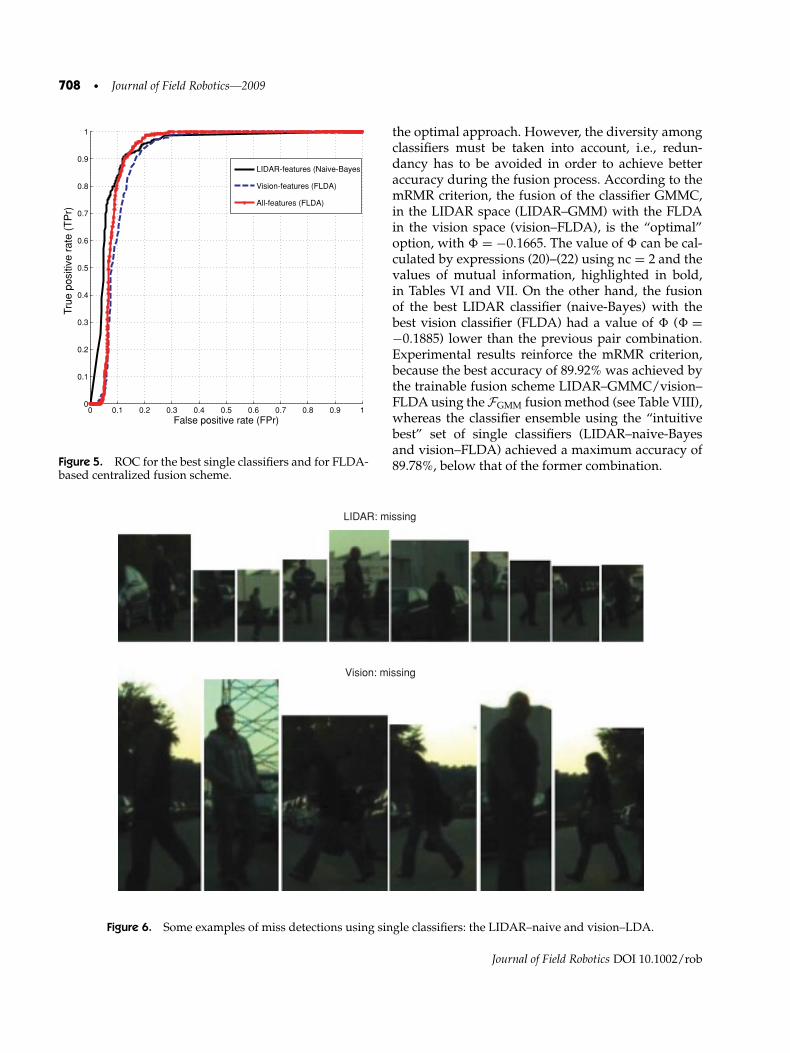
The centralized fusion scheme, in which all the fea-tures are concatenated in a single vector, was testedwith the FLDA, RBF–SVM, and MCI–NN classifiers.Table V summarizes the results obtained by the sin-gle classifiers and the classifier ensemble with thecentralized fusion structure. Regarding single classi-fiers, the naive-Bayes classifier had the best perfor-mance in the LIDAR space and the FLDA achievedthe best scores in the vision feature space. Regardingthe centralized scheme, the FLDA obtained the bestresults. ROC curves of the best single classifier and ofthe FLDA-based centralized fusion classifier are de-picted in Figure 5. Additionally, Figure 6 illustratessome missing detections using single classifiers in theLIDAR and vision feature spaces, giving some insightabout the missing occurrences.

Accuracy, BER, and AUC performance metricsare used throughout the paper. It is important to keepin mind that such metrics are calculated over all sam-ples presented on the testing data set; hence thosescores serve as a global indicator of the classifier per-formance. As a suggestion, we have selected a metricbased on a useful percentile of the AUC, up to 10% offalse positives, named AUC10%, because the optimaloperator point for ROC curves often does not occurout of that interval.

6.2. Classifier Selection for the DecentralizedFusion Scheme

Intuitively, the combination of the best LIDAR clas-sifier with the best vision classifier would result in



Figure 4. Some samples to illustrate the different conditions and situations in which the data set has been acquired.

Table V. Performance metrics: testing data set.

FLDA Naive–Bayes GMMC RBF–SVM MCI–NN

LIDAR-based features

Acc 0.786 0.883 0.875 0.840 0.861BER 0.154 0.108 0.130 0.204 0.124AUC10% 0.128 0.476 0.464 0.370 0.336TPr10% 0.304 0.835 0.842 0.688 0.765

Vision-based features

Acc 0.846 — — 0.841 0.813BER 0.172 — — 0.236 0.157AUC10% 0.178 — — 0.314 0.475TPr10% 0.63 — — 0.60 0.65

Fused features (all features): centralized scheme

Acc 0.880 — — 0.846 0.810BER 0.115 — — 0.231 0.226AUC10% 0.237 — — 0.324 0.198TPr10% 0.80 — — 0.60 0.60



0 0.1 0.2 0.3 0.4 0.5 0.6 0.7 0.8 0.9 10

0.1

0.2

0.3

0.4

0.5

0.6

0.7

0.8

0.9

1

False positive rate (FPr)

Tru

e p

osi

tive r

ate

(T

Pr)

LIDAR-features (Naive-Bayes

Vision-features (FLDA)

All-features (FLDA)

Figure 5. ROC for the best single classifiers and for FLDA-based centralized fusion scheme.

the optimal approach. However, the diversity amongclassifiers must be taken into account, i.e., redun-dancy has to be avoided in order to achieve betteraccuracy during the fusion process. According to themRMR criterion, the fusion of the classifier GMMC,in the LIDAR space (LIDAR–GMM) with the FLDAin the vision space (vision–FLDA), is the “optimal”option, with = −0.1665. The value of can be cal-culated by expressions (20)–(22) using nc = 2 and thevalues of mutual information, highlighted in bold,in Tables VI and VII. On the other hand, the fusionof the best LIDAR classifier (naive-Bayes) with thebest vision classifier (FLDA) had a value of ( =−0.1885) lower than the previous pair combination.Experimental results reinforce the mRMR criterion,because the best accuracy of 89.92% was achieved bythe trainable fusion scheme LIDAR–GMMC/vision–FLDA using the FGMM fusion method (see Table VIII),whereas the classifier ensemble using the “intuitivebest” set of single classifiers (LIDAR–naive-Bayesand vision–FLDA) achieved a maximum accuracy of89.78%, below that of the former combination.

LIDAR: missing

Vision: missing

Figure 6. Some examples of miss detections using single classifiers: the LIDAR–naive and vision–LDA.



Table VI. Mutual information among classifiers (redundancy).

LIDAR feature space Vision feature space

LDA Naive GMM SVM NN LDA SVM NN

LIDARLDA 1.000 0.602 0.621 0.585 0.615 0.574 0.590 0.570Naive 0.602 1.000 0.516 0.593 0.528 0.529 0.529 0.477GMM 0.621 0.516 1.000 0.625 0.609 0.661 0.661 0.608SVM 0.585 0.593 0.625 1.000 0.642 0.598 0.668 0.697NN 0.615 0.528 0.609 0.642 1.000 0.652 0.653 0.570

VisionLDA 0.574 0.529 0.661 0.598 0.652 1.000 0.710 0.622SVM 0.590 0.529 0.661 0.668 0.653 0.710 1.000 0.715NN 0.570 0.477 0.608 0.697 0.570 0.622 0.715 1.000

Table VII. Mutual information between classifiers and thetarget output (relevance).

Feature space Target output

LIDARLDA 0.498Naive 0.466GMM 0.642SVM 0.502NN 0.580

VisionLDA 0.686SVM 0.615NN 0.521

6.3. Decentralized Fusion Scheme:Classifier Fusion

The proposed decentralized fusion architecture wastested with different fusion methods, trainable andnontrainable ones, using the classifiers with maxi-mum relevance and minimal redundancy estimated

Table VIII. Performance metrics for the fusion strategies: testing data set.

Trainable methods Nontrainable rules

FLDA FNaive FGMM FSVM FNN FAvage FMax FNprod

Acc 0.894 0.897 0.899 0.877 0.890 0.878 0.859 0.878BER 0.109 0.108 0.096 0.124 0.102 0.122 0.109 0.122AUC10% 0.391 0.460 0.465 0.412 0.421 0.282 0.178 0.197TPr10% 0.861 0.892 0.912 0.855 0.850 0.684 0.633 0.710

over the training data set (LIDAR–GMMC andvision–FLDA).

Here, the most demanding task is the selectionof the 15 possible combinations, five classifiers in theLIDAR space and three in the vision space. Thisaspect reinforces the need to avoid heuristic, orforce-brute, methods and to consider a mutualinformation-based approach to aid in such labor, asdescribed in the preceding section.

Once the most relevant and less redundant pairof classifiers has been selected, the set of proposedtrainable fusion techniques, denoted FLDA, FNaive,FGMM, FSVM, and FNN, and the nontrainable rules,FAvage, FMax, and FNprod, were applied over the test-ing data set. The results concerning each fusion tech-nique are shown in Table VIII, and correspondingROC curves are depicted in Figures 7(a) and 7(b).

7. CONCLUSION

Most of the works on pedestrian and on-road ob-ject detection using vision and LIDAR (see Table Ifor some relevant cases) employ a LIDAR to detect



0 0.1 0.2 0.3 0.4 0.5 0.6 0.7 0.8 0.9 10

0.1

0.2

0.3

0.4

0.5

0.6

0.7

0.8

0.9

1


Tru

e p

osi

tive r

ate

(T

Pr)

F-Avage

F-Max

F-Nprod

0 0.1 0.2 0.3 0.4 0.5 0.6 0.7 0.8 0.9 10

0.1

0.2

0.3

0.4

0.5

0.6

0.7

0.8

0.9

1


Tru

e p

osi

tive

ra

te (

TP

r)

F-LDA

F-Naive

F-GMM

F-SVM

F-NN

(a) ROC: fusion with nontrainable rules (b) ROC: fusion with trainable methods

Figure 7. The ROC using the decentralized fusion scheme.

objects and to generate target hypotheses inside thecamera FOV, whereas a vision-based classifier is incharge of object validation or final classification. Thepresent work contributes a sensor fusion strategycomposed of centralized and decentralized fusionschemes. In the former the fusion process occurs atthe feature level followed by a single classifier ap-plied over the whole feature vector, and in the latterthe pair of classifiers with max-relevance and min-redundancy is fused by means of a set of trainablemethods and nontrainable rules to improve the finalclassification stage.

Regarding the experimental results, the follow-ing conclusions can be highlighted:

1. Trainable fusion methods: These fusion tech-niques got better results than the usual non-trainable rules, evidencing the feasibility ofthe proposed methods.

2. mRMR criteria: To prevent redundancy andto take advantage of the classifier diversity,avoiding empirical approaches, this methodis very useful during the classifier selection,aiding in choosing the better combination interms of mutual information.

3. LIDAR-based detection missing: The miss-ing detections for the LIDAR-based classi-

fiers are related mainly to the range distanceto the object; the farther the object is from theLIDAR, the less range information is avail-able and consequently the system is prone tofalse-negative classifications. Moreover, sit-uations in which pedestrians appear veryclose to each other or close to or betweenother objects (especially cars) originate prob-able missing detections.

4. Vision-based detection missing: Most ofthe cases occur on low-contrast imagesand when the ROI background has intensetexture.

5. Fusion strategy: The proposed fusion strate-gies achieved higher performance than thesingle classifiers, for which the decentralizedscheme obtained the best result.

Moreover, in terms of practical applications, as the fu-sion schemes do not depend entirely on a single sen-sor space, this brings more robustness and safety tosystems employing such detection schemes.

ACKNOWLEDGMENTS

This work is supported in part by the Fundacaopara a Ciencia e a Tecnologia de Portugal (FCT)



under grant PTDC/EEA-ACR/72226/2006. C. Pre-mebida is supported by the FCT under grant SFRH/BD/30288/2006 and O. Ludwig under grant SFRH/BD/44163/2008. The authors would like to thankthe reviewers for their valuable comments andsuggestions.

REFERENCES

Abe, S. (2005). Support vector machines for pattern classi-fication (Advances in Pattern Recognition). Secaucus,NJ: Springer-Verlag New York, Inc.

Arras, K., Mozos, O., & Burgard, W. (2007, April). Us-ing boosted features for the detection of people in 2Drange data. In 2007 IEEE International Conference onRobotics and Automation, Rome (pp. 3402–3407).

Cheng, H., Zheng, N., Zhang, X., Qin, J., & van deWetering, H. (2007). Interactive road situation analy-sis for driver assistance and safety warning systems:Framework and algorithms. IEEE Transactions on In-telligent Transportation Systems, 8(1), 157–167.

Dalal, N., & Triggs, B. (2005, June). Histograms of orientedgradients for human detection. In Proceedings of the2005 IEEE Computer Society Conference on ComputerVision and Pattern Recognition (CVPR’05), Washing-ton, DC (vol. 1, pp. 886–893). San Diego, CA: IEEEComputer Society.

Douillard, B., Fox, D., & Ramos, F. (2007, October). A spatio-temporal probabilistic model for multi-sensor objectrecognition. In IEEE/RSJ International Conference onIntelligent Robots and Systems, 2007. IROS 2007, SanDiego, CA (pp. 2402–2408).

Gandhi, T., & Trivedi, M. M. (2007). Pedestrian protectionsystems: Issues, survey, and challenges. IEEE Transac-tions on Intelligent Transportation Systems, 8(3), 413–430.

Guivant, J. E., Masson, F. R., & Nebot, E. M. (2002). Simul-taneous localization and map building using naturalfeatures and absolute information. Robotics and Au-tonomous Systems, 40(2–3), 79–90.

Hall, D., & Llinas, J. (1997). An introduction to multisensordata fusion. Proceedings of the IEEE, 85(1), 6–23.

Hwang, J. P., Cho, S. E., Ryu, K. J., Park, S., & Kim, E. (2007,September). Multi-classifier based lidar and camera fu-sion. In Intelligent Transportation Systems Conference,2007. ITSC 2007, Seattle, WA (pp. 467–472). IEEE.

Lowe, D. G. (2004). Distinctive image features from scale-invariant keypoints. International Journal of Com-puter Vision, 60(2), 91–110.

Ludwig, O., Delgado, D., Goncalves, V., & Nunes, U. (2009,October). Trainable classifier-fusion schemes: An ap-plication to pedestrian detection. In Intelligent Trans-portation Systems Conference, ITSC 2009, St. Louis,MO. IEEE.

Ludwig, O., & Nunes, U. (2008, October). Improving thegeneralization properties of neural networks: An ap-plication to vehicle detection. In 11th InternationalIEEE Conference on Intelligent Transportation Sys-tems, 2008. ITSC 2008, Beijing (pp. 310–315).

Mahlisch, M., Schweiger, R., Ritter, W., & Dietmayer,K. (2006, June). Sensorfusion using spatio-temporalaligned video and lidar for improved vehicle detec-tion. In 2006 IEEE Intelligent Vehicles Symposium,Tokyo (pp. 424–429).

Pangop, L. N., Chapuis, R., Bonnet, S., Cornou, S., &Chausse, F. (2008, September). A Bayesian multisensorfusion approach integrating correlated data appliedto a real-time pedestrian detection system. In IEEEIROS2008 2nd Workshop on Perception, Planning andNavigation for Intelligent Vehicles, Nice, France.

Peng, H., Long, F., & Ding, C. (2005). Feature selec-tion based on mutual information criteria of max-dependency, max-relevance, and min-redundancy.IEEE Transactions on Pattern Analysis and MachineIntelligence, 27(8), 1226–1238.

Premebida, C., & Nunes, U. (2005, April). Segmentationand geometric primitives extraction from 2D laserrange data for mobile robot applications. In Proceed-ings of 5th National Festival of Robotics, ScientificMeeting (ROBOTICA), Coimbra, Portugal.

Premebida, C., & Nunes, U. (2006, September). A multi-target tracking and gmm-classifier for intelligent vehi-cles. In Intelligent Transportation Systems Conference,2006. ITSC ’06, Toronto, Canada (pp. 313–318). IEEE.

Spinello, L., & Siegwart, R. (2008, May). Human detectionusing multimodal and multidimensional features. InIEEE International Conference on Robotics and Au-tomation, 2008. ICRA 2008, Pasadena, CA (pp. 3264–3269).

Streller, D., & Dietmayer, K. (2004, June). Object track-ing and classification using a multiple hypothesis ap-proach. In 2004 IEEE Intelligent Vehicles Symposium,Parma, Italy (pp. 808–812).

Szarvas, M., Sakai, U., & Ogata, J. (2006, June). Real-time pedestrian detection using lidar and convolu-tional neural networks. In 2006 IEEE Intelligent Vehi-cles Symposium, Tokyo (pp. 213–218).

Tuzel, O., Porikli, F., & Meer, P. (2006, May). Region covari-ance: A fast descriptor for detection and classification.In Proceedings of 9th European Conference on Com-puter Vision, Graz, Austria (pp. 589–600).

Tuzel, O., Porikli, F., & Meer, P. (2007, June). Human de-tection via classification on Riemannian manifolds.In IEEE Conference on Computer Vision and Pat-tern Recognition, 2007. CVPR ’07, Minneapolis, MN(pp. 1–8).

Vapnik, V. N. (1998). Statistical learning theory. New York:Wiley.

Xavier, J., Pacheco, M., Castro, D., Ruano, A., & Nunes,U. (2005, April). Fast line, arc/circle and leg detectionfrom laser scan data in a player driver. In Proceedingsof the 2005 IEEE International Conference on Roboticsand Automation, 2005. ICRA 2005, Barcelona, Spain(pp. 3930–3935).

Zhang, Q., & Pless, R. (2004, September). Extrinsic cali-bration of a camera and laser range finder (improvescamera calibration). In Proceedings. 2004 IEEE/RSJ In-ternational Conference on Intelligent Robots and Sys-tems, 2004. (IROS 2004), Sendai, Japan (vol. 3, pp. 2301–2306).


LIDAR and Vision-Based Pedestrian Detection System - …home.isr.uc.pt/~cpremebida/files_cp/LIDAR...

Documents

Transcript of LIDAR and Vision-Based Pedestrian Detection System - …home.isr.uc.pt/~cpremebida/files_cp/LIDAR...