R- D-AI57 722 HIGH REYNOLDS NUMBER NAVE FORCE INVESTIGATION IN A WAVE 141#FLUME(U) OREGON STATE UNIV CORVALLIS DEPT OF CIVILI ENGINEERING R T HUDSPETH ET AL. MAR 85 NCEL-CR-B5. 664UNCLASSIFIED N62474-82-C-08295 F/G 26/4 N

I lfffllff~fflllff

11111 1111

NAt4a L aLMWA OF STAMMRDSWainOCOp" RtSOU TESTrn 014AT

of 11 .** *..

i J.

CR 85.004

NAVAL CIVIL ENGINEERING LABORATORYPort Hueneme, California

4CIeEtiu~WLn E

Sponsored byDEPARTMENT OF INTERIORMINERALS MANAGEMENT SERVICENAVAL FACILITIES ENGINEERING COMMAND

HIGH REYNOLDS NUMBER WAVE FORCE INVESTIGATIONIN A WAVE FLUME

March 1985

An Investigation Conducted by:Ocean Engineering ProgramCivil Engineering DepartmentOregon State UniversityCorvallis, OR 97311

~DTIC

N62474-82-C08295 L CT -

ELECTELA S JU 1 7198M

~ Approved for public release; distribution is unlimited.

85 06 28 053

.- - -- -. . o . .,O o o . . . . °... .. . . . . . . . . . . • ,•o-

*1*1

2 a

" , .;_ .... o

0 I, ! i i 0M

.

E

E E~ E E

I _ I II I I I 1-i n_

ot 1 li' f6

I I S2 ?I

j. 2

-W. o. " . . .- io. -.A . . ._ r - -. -o , -ri 0 . -r, j r~ - . .. .- r r. d. yo -" .. ... r _ c. .. . i .. . . . . .r-%i

Unclassi fiedSECURITY CLASSIFICATION OF THIS PAGE (WheI )#1. Fntrrd)

READ INSTRUCTIONSREPORT DOCUMENTATION PAGE BEFORE COMPLETING FORM

1. REPORT NUMER Ii OVT ACCIES11ON NO.IRCPEV AO UERA

CR 85.004 LW 441 TP

4. TITLE f(.d S.b118.) S. IYPE OF REPORT & PERIOD COVERED

High Reynolds Number Wave Force FinalInvestiqation in a Wave Flume Sep 1982-Feb 1985 1IL

6 PERFORMING ORG. REPORT NUMBER

AUTNOR(.) 8. CONTRACT OR GRANT NUMBER(.)

Robert T. Hudspeth and John H. Nath N62474-82-C08295

S. Q RFORMI L. OR, NIZATI N NAk AND ADDRESS 10 PROGRAM ELEMENT. PROJECT. TASK

OceaO En ineering rogram, Civil Engi- AREA6 WORK UNIT NUMBERS

neering 8ear.menht YF60.534.091.01 A352 "-

UreooSta~bni~ersityCorva/ ii qiUKN/1/ _______

II CONTROLLING OFFICE NAME AND ADDRESS 12. REPORT DATE H

Naval Civil Engineering Laboratory March 1985Port Hueneme, CA 93043 22. NUMBEROFAS S220

14 MoN TORI G C MEr AffIPESS(Itdlcn .enI o t aIon a Office) IS SECURITY CLASS. (Of thi .e o#f)Dept Olflnteyrior, inera9s ,TmV erv .Tech Assessment & Research Proaram Unclassified647 National Ctr, Reston, VA 22091 ISO. DECLASSIFICATION DOWNGRADING

Nay Fac Enar Cmd, Alexandria, VA 22332 SCHEDULE .16 DISTRIBUTION STATEMENT (.f rhi. RpoI)

Approved for public release; distribution is:-unlimited.

17 DISTRIBUTION STATEMENT (of Ph. obefrsce *HI,,d in Block 20. it diffl~I ft-e ReIPeot)

I0 SUPPLEMENTARY NOTES

W' KEY WORDS (CoAI$nue . .'*e. esd. it n- .c.y -d Idnflfy by block nlbe"l)

iWave forces; j-xperiment, ]arpe scale; Morison equation, ighReynolds numbe'ri cylinders, in-line forces; transverse forces.-

20 ABSTRACT (CitiIhnIfb . ....... yde , o d id.ln.fy by bloc* n-b.t)

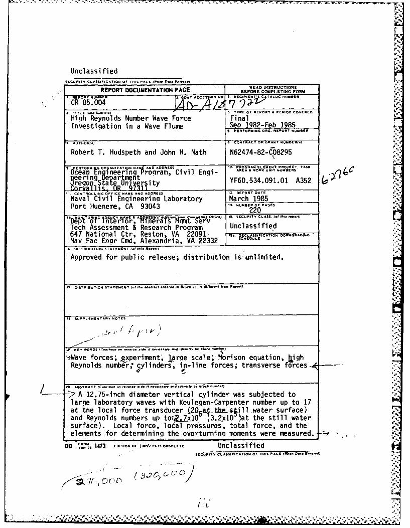
- A 12.75-inch diameter vertical cylinder was subjected tolarge laboratory waves with Keulegan-Carpenter number up to 17at the local force transducer t205 a. he ill .water surface)and Reynolds numbers uD t (3.?x102at the still watersurface). Local force, loa-l pressures-, total force, and theelements for determining the overturning moments were measured.

DD 12' 1473 EDITION F 1 NV , IS O.SOLETE UnclassifiedSECURITY CLASSIFICATION OF THIS PAGE (a~on Dale EnIeo.d)

(IL.

" ... • " " :-,-" . . . '."" , " " 'I"" " " " " " " " " " " .

UnclassifiedS SCCUPITV CLASUPIICATION OP

e YIis PA09(whaft Does ER1o"49)

--The purpose was to produce a high quality data set in thewave regime where both the velocity and the acceleration-dependent components of the wave forces are important. Itwas found that the forces were more acceleration-dependentthan oriqinally anticipated.

The local forces were predicted quite well with the two-term Morison equation using the kinematics from the measure-ments, the linear, and the stream function wave theories. Thebest predictions used the measured kinematics. ,

ircssionFoins a iFUmic TAB

Justifli.ti

Avallb~Ity Codes

Dist speial

Unclassi fiedSECUmI' CLASSIrCAT,O o T1 PAOEG 'WC 0'. FVS 'e- e)

/v'

TABLE OF CONTENTS

Page

1.0 ABSTRACT 1

2.0 INTRODUCTION 3

2.1 Background 3

2.2 Purposes of Test Program 5

2.3 Scope 6

3.0 EXPERIMENT SETUP AND PROCEDURES 9

3.1 Wave Research Laboratory 9

3.2 Experimental and Data Acquisition Equipment 9

3.2.1 Test Cylinder 93.2.2 Force Beam Gauging 123.2.3 Data Acquisition 15

3.3 Test Procedures 16

3.3.1 Calibrations 163.3.2 Test Plan 19

4.0 DATA ANALYSIS 21

4.1 Record Format and Filtering 22

4.2 Data Processing 29

4.2.1 PROGRAM WAVE8 304.2.2 PROGRAM FDATA5/FD5A 324.2.3 PROGRAM LABT4 33

4.3 Random Waves 39

4.3.1 PROGRAM WAVER 404.3.2 PROGRAM FDATAR 404.3.3 PROGRAM LABT4 41

5.0 SIMMARY OF RESULTS 43

6.0 CONCLUSIONS 45

7.0 REFERENCES 49

8.0 ACKNOWLEDGEMENTS 51

9.0 TABLES 53

10.0 FIGURES 93

11.0 APPENDIXA"

11.1 Druck Pressure Transducer Specifications A3

11.2 Parametric Dependency of Force Coefficients onDean Number A9

11.3 FDATAR A13

S.

• -q.. .. .:.. .,... .... ...-/ ...... .-. . ..-,-........... , ...- ). ......--.. ; .. ., -.-.. :...-..- ,V,.

1.0 ABSTRACT

A 12.75-inch diameter vertical cylinder was subjected to large

"" laboratory waves with Keulegan-Carpenter number up to 17 at the

local force transducer (20 at the still water surface) and Reynolds

numbers up to 2.7xi0 5 (3.2x10 5 at the still water surface). Local

force, local pressures, total force, and the elements for determin-

ing the overturning moments were measured. The purpose was to

produce a high quality data set in the wave regime where both the

velocity and the acceleration-dependent components of the wave

forces are important. It was found that the forces were more accel-

eration-dependent than originally anticipated.

The local forces were predicted quite well wiry the two-term

Morison equation using the kinematics from the measurements, the

5' linear, and the stream function wave theories. rhie best predictions

used the measured kinematics.

p

1-1

-- .-... '. -' ... ... .. , - .- . - ,- °- ... . . . .. . . . . . . . ..- , , ... . .. . .,.. . . . . -.. -.. . . . . . . . . . ,-._.. . . . . . . .. . . . . - . .

2.0 INTRODUCTION

2.1 Background

On 27 September 1982 a contract was established between the

Naval Civil Engineering Laboratory (NCEL), Port Hueneme, California,

and Oregon State University (OSU), to conduct an experiment pertain-

ing to wave forces on a 12.15-inch diameter vertical cylinder. The

design work for the equipment began in October 1982, and the equip-

ment was delivered on site in February 1983. Ihe laboratory tests

were performed in the period from 12-26 April 1983 and data analyses

were completed during the Fall 1983. these final data analyses were

made possible by a modification to the original NCEL contract with

finding from the Minerals Management Service (MMS) through NCEL.

The Morison equation relating wave forces on vertical cylinders

is given in the following equation. the force per unit of cylinder

length, f, is expressed by

0 D2

F= cd ?u(t)lu(t)I + Cm x_ f_ t(2.1-1)

where Cd and Cm are the empirically determined drag and inertia

coefficients, respectively (Cm = 1 + Ca, where Ca is the added mass

coefficient), D is the cylinder diameter, p is the mass density of

the surrounding water, u(t) is the horizontal water particle veloci-

ty, and ;(t) is the local fluid acceleration au/at.

Many data have been generated from experiments by many investi-

gators to determine the drag and inertia coefficients as functions

of the Keulegan-Carpenter number, K (= UmT/D, where Um is the maxi-

, ; mum water particle speed and T is the wave period), and the Reynolds

-3-

... . .

number, R ( Umd/v, where v is the kinematic viscosity of the

water). However, many reportings have been questioned for one

reason or another and only a few have very reliable values for these

force transfer coefficients. One reliable source is from planar

oscillatory flow laboratory experiments. However, they are limited

because the flow is not truly that of waves. Other data sources

have their own limitations. For example, field experiments rely

heavily on current measurements that are made at some distance from

the force transducer and wave theory is ultimately used to extend

the measurement to the force transducer location. lo our knowledge,

no set of well-documented, thoroughly instrumented measurements have

been made in a truly controlled wave condition and reported on in

the open literature.

Even the data from planar oscil.atory flow have some scatter

and indicate that Eq. 1 may be improved to reproduce well the forces

acting on a cylinder within certain ranges of K. Therefore,

Sarpkaya (1981) suggested the use of a so-called four-term Morison

equation, wherein two terms are added to Eq. 1 to take into account

energies in the force spectrum that occur at the Jrd and bth harmon-

ics of the fundamental wave frequency. The coefficients for the

added two terms can be determined, essentially, from the drag and

inertia coefficients as determined from the two-term equation.

The form of the four-term MOJS equation used for this work is

-4-

Ft . ", -""-""'' ." -' ' -" ." .," ",," ". "".. .""" -.- """". .'"' "" . ; " "-' ' -' '"- '": . " "

".' ," -' . . -- ."- '. .- ." '"""

",dl " " " " " ' -" .. .": " . .'. . : : " 5 " .." "' " ',,* & m , i''mW ii i....l ',a

. '. ._.- -. . -- -- *_.. . .... .. .~.-. • -. . .. .. ... ° . '.- -... . . . . .

O2 G~) pDU2F -Ca D~~~ +CLmt) + M[Ac3Bcexp(Ccro)]

od u(t) Iu(t) I + Cm 2A + pDU2

cos{3 ut-A A +13 exp (C m [Ac5+Bc5exp(Cc5) ]

cos { t - A-1 /2 [A 5+ B * 5 exp(C 5)] } (2.1-2)

where a = (K - 12.5)2, ,,, = 2w/T, K = UmT/D, x = (Cn - Cm)/KCd (C is

the potential flow value--for a cylinder, C* = 2.9), andm

Ac3 =0.01 Bc3 = 0.10 Cc3 = 0.08

A,3 = -0.05 - -0.35 C,3 -0.04

Ac5 = 0.0025 Bc5 = 0.053 Cc5 = -0.06

A = 0.25 BO5-- 0.60 C 5 = -0.02

On ly two terms were a'ded to the Morison equation because the

spectrum analyses of the residues from the U-tube experiments

* (Sarpkaya, 1981) showed appreciable energy from only these two

higher ordered terms.

2.2 Purposes of rest Program

The major purpose of this program was to provide a high quality

set of data of force measurements and pressure measurements for a

vertical smooth cylinder of appreciable size (12.75-inch diameter)

" in real waves with a reasonable range of Keulegan-Carpenter and

Reynolds numbers so that different methods of analyses can be exam-

ined (for this and future efforts). Also required were comparisons

of the force transfer coefficients from different methods of analy-

sis and comparisons of forces, using the differently derived coeffi-

cients.

-5-

2.3 Scope

The work entailed constructing a 12.75-inch diameter test

cylinder equipment, conducting the laboratory model tests, recording

and analyzing the data, and production of the reports. The test

cylinder equipment was of all new construction. Local forces, total

forces, and the elements for determining the overturning moments

were measured. In addition, eight pressure transducers measured

peripheral time-dependent pressures around the center of the local

force transducer. Wave water particle velocities were measured

opposite the center of the local force transducer, in line with the

wave axis (crests). he water surface profi;e was measured in line

with the wave axis and the center of the cylinder.

A minimum of 26 runs were required to satisfy the requirements

of the statement of work (SOW). lowever, a total of 4/ runs were

made since testing time did permit them. Data from 26 runs were

analyzed as required in the SOW. len waves in a sequence were

recorded from which eight were later extracted for the analysis.

The eight wave periods, beginning at any time in the sequence,

allowed for seven complete peak-to-peak waves to be defined.

The force transfer coefficients, Cd and Cm, were derived with

least square methods, using linear and stream function wave theories

and the measured kinematics. In addition, Cd and Cm were determined

from the Wave Project II di',., where Cm is constant and Cd varies

with time through the wave cycle (lidspeth, et. al. 19/4), and from

Sarpkaya's U-tube results (Sarpkaya, 1981). The predicted forces

were then conared against the measured forces, wherein the pre-

dicted forces included calculations using Eqs. 2.1-1 and 2.

-6-. . ... . . . . . . . . . . . ....

i' .' t ... .. i .. . . !.. . . ' i "- i t ,_ ,',.. . . . . . .. . . . . . . . . . . . . . . . . . .- ".-.. . . . . . . . . . . . . T "

In summary, the analysis included 12 combinations of time-

dependent force determinations. Using the kinematics from each of

the linear wave theory, the stream function wave theory, and the

measured kinematics, the time-dependent forces were determined for

both the 2-term and the 4-term Morison equations, using Cd and Cm

determined from the least squares method, Wave Project II data, and

the U-tube data.

-7-

3.0 EXPERIMENT SETUP AND PROCEDURES

3.1 Wave Research Laboratory

The experimental work was done in the O.H. Hinsdale Wave

Research Laboratory at Oregon State University (WRL). The overall

length of the wave flume is 340 ft., of which 129 ft. constitute the

length in which tests can be performed well beyond the evanescent

modes of the wave board and in front of the toe of the beach. The

location of the test cylinder in the WRL is shown in Fig. 3-1.

Good, repeatable waves can be produced ranging from a high frequency

of 1.0 Hz to a low of about 0.12 Hz. For these tests, the wave fre-

quency range was from 0.5 Hz to 0.12 Hz. Up to 16 channels of

information were recorded digitally in real time on a PDP 11 com-

puter. Other channels of information were recorded on an analogue

tape recorder and then digitized at a later time.

3.2 Experimental and Data Acquisition Equipment

3.2.1 Test Cylinder

The design of the test cylinder required that it be stiff for

the applied loads so that the natural frequency of the lowest mode

would be relatively high with respect to the forcing frequencies.

From impulse response tests, where the cylinder was hit with a

rubber hammer and the time response was measured by strip chart

recorder, the local force transducer demonstrated a natural frequen-

cy of 8.2 Hz when submerged. The highest wave frequency in this

test was 0.5 Hz. On some runs, a distinct transverse force was

experienced, due to vortex shedding, that had frequencies higher

-9-

TA- %7 -1 77--77a .7.I!

than the wave frequency by up to approximately three times. In

addition, other turbulences may cause transverse forces. The ampli-

tude spectra for transverse forces in Vol. II were examined for

maximum significant frequencies. An approximate value of 1.5 Hz was

determined as a conservatively high estimate, even though the ampli-

tudes therefrom were fairly small. Some other very small energies

exist at 5.0 Hz and at 8.0 Hz for the center force, east direction

(probably due to the vibration of the local force transducer from

near-impact loads in steep waves). Thus, the largest ratio of

importance of excitation frequency to transducer frequency was about

1.5/8 = 0.19. The largest ratio of fundamental wave frequency to

transducer frequency was .5/8 = .062. 1herefore, vibrations of the

local force transducer had a negligible effect on the measurements

as can be seen in any reference on dynamics for the response curve

of a one-degree-of-freedom vibrator. rhe signals were also filtered

-. with a two-pole Butterworth filter with a cutoff frequency of 8

Hz. However, the signals were recorded filtered and unfiltered in

case future reference is to be made to the unfiltered signals.

Another design criterion was to size the test cylinder so that

the component parts could be handled relatively easily at the wave

a flume. It was decided to provide a stiff inner core structure with

a removable shell surrounding it.

Figure 3-2 gives the general concept of the test cylinder.

Figures 3-3 and 4 are photos of it during installation, where Fig.

3-4 has only one-half of the lower skin in place. Figure 3-5 shows

the strain gauges on the bottom support; Fig. 3-6 shows the bolt-

-10-

!

down arrangement at the bottom; and Fig. 3-7 shows how the bottom

skin covered the supporting core.

The upper support consisted of a 1.5-inch round stainless steel

rod, 30 inches long, inserted into roller bearings and supported at

-. its upper end with a U-joint identical to the one at the bottom

support, as shown in Fig. 3-2. Thus, the structure was completely

statically determinate and no longitudinal forces could be applied

to the structure from temperature variations or other longitudinal

stresses from construction because of the upper roller support.

It was necessary to design the local force transducer for much

smaller forces than would be measured at the top and bottom trans-

ducers and to make it individually statically determinate and free

from the small deflections of the central structure. Details of the

local force transducer (LFF) are shown in Figs. 3-8 and 9. Photos

of the strain bar supports and the interior of the LFT are given in

Figs 3-10 and 11.

The test cylinder was supported at the upper end by an 8x12

steel tube that spanned the 12 ft. clear distance between the wave

flume walls, to which it was securely bolted. fhe wave profiler was

mounted in this beam with the center of the profiler in line with

the center of the test cylinder, perpendicular to the wall. It was

Amounted 3 ft. from the east wall, mid-way between the wall and the

cylinder center line. A Marsh-McBirney current meter was mounted

with the sensing elements directly under the wave profiler at a

level of 3.7 ft. below the still water surface--the same level as

. the center of the local force transducer. A second Marsh-McBirney

'I

-11-

!. , " •", .- °%° °. ,• . . . -•. . . . . .. . . . . * . . . . . . ..a

I r r r r r , ° I l m j , , . ,-.r ,. - - . - . . . . . . . . .

current meter was mounted directly in line with the first one, but

on the opposite (west) wall. The sensors of the second meter were

about 1.2 ft. from the face of the west wall.

The test cylinder was carefully assembled so that the center

line was vertical. The local force transducer was separated only

1/16-inch from the rest of the cylinder, but the surface was slight-

ly out of alignment with the smooth cylinder skins. Figures 3-12

and 13 show the best and worst alignments. Several measurements

were made of the misalignments and they are summarized in Table 3-

1. The table shows the LFI was slightly larger in diameter than the

adjoining test cylinder by 0.7 mm, which had a negligible influence

on the resulting measurements.

After the Druck pressure transducers were installed and the LFT

was mounted, the surface around the pressure transducers was filled

with a paint-like substance and sanded smooth with the surrounding

cylinder surface.

3.2.2 Force Beam Gauging

Forces were measured with strain gauge force dynamometers.

Metal foil strain gauges were used of 120 ohms each. The gauging

stations are referred to as the top gauge, the local force trans-

ducer, and the bottom gauge. Ihe top and bottom gauges were wired

as shown in Fig. 3-14.

5The local force transducer was wired as shown in Fig. 3-15.

Each of the four 5/16-inch square support beams had four gauges,

intending to have two complete circuits for each of the in-line and

transverse directions. However, small torsional loads from the

-12-

-. 21

calibration string gave inconsistent results so the two in-line and

two transverse circuits were added together. This action nullified

any influence on the readings from torsional loads. All strain

gauge bridging was conditioned with Vishay signal conditioners.

The Vishay strain gauge conditioner contains two sections. The

first is a precision adjustable voltage regulator. The output of

the regulator is used as the excitation for the strain gauges. For

this work it was adjusted for 10.00 volts. The exact value is not

critical if the instrument to which the gauges are attached is cali-

brated at that voltage, whatever it is. The second section includes

several stages of amplification to the very small voltage changes

coming from the strain gauge bridge, ihe first stage is a differen-

tial-type amplifier which will detect and amplify only voltage

potentials which exist between the two return leads from the

bridge. Any potential between ground and one lead or in common with

both will not be amplified. This last stage then provides isolation

from many noise problems. The other stage of the amplifier section

provides further adjustable gain which can be set to obtain a usable

voltage output within a desired range from the conditioner box.

Auxiliary circuits in the conditioner provide bridge balancing

circuitry to nullify any static offset so that a maximum gain may be

used for very small bridge outputs. Circuitry for different types

of bridges and amplifier adjustments for best output are included.

Outputs from the conditioners were input to the Rockland 8.0 Hz low

pass double pole filters.

-13-

Selected outputs were then passed into summing-type inverting

operational amplifiers with a gain of very nearly -1.0. The exact

value, again, does not matter if the instrument is calibrated using

the output of the last piece of electronic equipment. The summing

amplifier has a very large bandpass from DC to several thousandhertz and therefore will cause no measurable phase shift at our

frequencies.

Some of the characteristics of the general operation amplifier

are that it has a very high input impedance and low input current

(useful to prevent loading of the preceding instrument). Because of

this very high input impedance, the current drawn by the 'op amp' is

negligible and therefore point 'A' (see Figure 3-16) is very nearly

v at ground potential, or zero volts. Because of this, the current

drawn through the input resistor R1 and R2, Ii, is equal to the

current through Rf, the feedback resistor. Upon solving for these

relations (without including every step here), we find that Vo/Vin =

-Rf/Ru . Our Rf/R i is set to be 1.0.

In the more specific case of the summing op amp, the current Ii

is the sum of the currents Irl and 1r2 and so we arrive at the rela-

tion (again without showing all the intermediate steps):

-V /Rf = V1/R + V2/R 2 (3.2.2-1)

In our case RI/Rf = 1.0 and R2 /Rf = 1.0 and so we have as a final

output the sum of the inputs:

-Vo 1 1 + V2 (3.2.2-2)

-14-

.i .'.o.- -.. .' ,P , 4 ",A, ", ' .- , ' --" ." - "" . .A*% A-.A. 'd. " i ilil i Liia, A*,li bd lm

This being the last instrument we have our final output voltage

corrected for torsion and other unwanted bending moments and with

very reduced noise ready to be digitized by the conputer.

In summary, Fig. 3-17 shows the test cylinder with only one of

the four cylinder skins attached to the core beam. Figure 3-18

shows three of the four skins bolted on. Figure 3-19 shows the

completed assembly just prior to testing. The west wall Marsh-

McBirney current meter is shown on the left side and east wall

installation is shown on the right side of the photograph.

3.2.3 Data Acquisition

The signals were routed as shown in Fig. 3-20. A maximum of 16

channels of information can be digitized simultaneously with the

POP-11 cooputer. The remaining channels were recorded on analogue

tape for digitizing at a later time. The analogue tape introduced

additional high frequency noise so the signals therefrom were again

filtered prior to digitizing.

The analogue filter is a two-pole Butterworth filter manufac-

tured by Rockwell. The digital recording was done with a POP-i

minicooputer. The analogue tape recorder was a Bell and Howell

model CPR-4010. The digital information was stored on an Ul-track

mag tape and a copy of all data recorded were provided to NCEL.

_ In order to help synchronize all channels in real time, a 5-

volt step function signal was generated by the computer and recorded

on one channel. rhis 5-volt "switch" was activated at the start of

digital recording. This signal was also recorded on the analogue

tape. The data analysis used this "switching" technique to help

phase all information.

-15-* : .' ., , ' C.' '-. -- . *. -,'-."'* .- "'. "-'.*> - ' :, " -. . -''- . *.,-- .'.'.* ;, --- ', '' '''''-:r ' * .

3.3 Test Procedures

3.3.1 Calibrations

The completed cylinder was calibrated in four force directions

corresponding to the four points of the compass. In addition, one

horizontal diagonal calibration was made to illustrate independence

between the N-S and E-W force measurements. Two ranges of forces

were used for the top and bottom force transducers in order to check

their linearity. One range had a maximum load of 201.44 pounds and

the other was 16.56 pounds, as shown in Table 3-2. Force calibra-

tions were made at one or more of the five elevations as shown in

Fig. 3-21. One measurement was made with the forces applied simul-

taneously at locations 2, 3, and 4. These were compared with force

calibrations at position 3 alone. The purpose of this was to

determine if distributed loads, which create bending in the overall

structure, would influence the force measurements at position 3

alone. When the forces were applied simultaneously to positions 2,

3, and 4, it is designated as the XXX test. In that case, the light

calibration was applied at position 3 while the heavy calibration

loads were applied to positions 2 and 4 with approximately the steps

indicated in Table 3-2. (This loading at positions 2 and 4 could be

approximate since it was only intended to provide a significant

general bending of the core beam to see if it influenced the cali-

brations of the LFT.) When the force was applied to position 3

only, it is designated as the OXO calibration. It was found that

force measurements from the local force transducer were independent

of the general loading on the cylinder. Of course, during tests the

-16-

* I"%*.t~~ .

sensors for the local force transducer and the bottom force trans-

ducer were submerged. They were therefore calibrated in the

submerged condition.

* The XXX calibration arrangement is shown in Fig. 3-22. Figure

3-23 shows a calibration in progress at position 5 (submerged).

When calibrating at position 3 in the north or south directions, it

was necessary to provide a horizontal truss at the correct level to

take the horizontal and vertical thrust from the calibration

loads. It is shown in Fig. 3-23.

Linear regression analysis was used to obtain the calibration

coefficients. The measured calibration data values, fi, were ap-

proximated by a linear relation to the measured voltage, xi,

according to

fi = m xi + b; i = 1,2,..., N (3.3.1-1)

where the slope, m, and the intercept, b, were determined by a best

least squares analysis. [he correlation coefficient, R was computed

by

[LC fixi - fiIxi/N132

R2 Z 1 (3.3.1-2)

E f2. - (Efi) INJLE x. - (ixi)Z/N]i I i

and is a measure of the goodness-of-fit of the two regression coef-

ficients since 0.0 4 R2 < 1.0. If R were identically equal to 1.0,

the data would be perfectly linear.

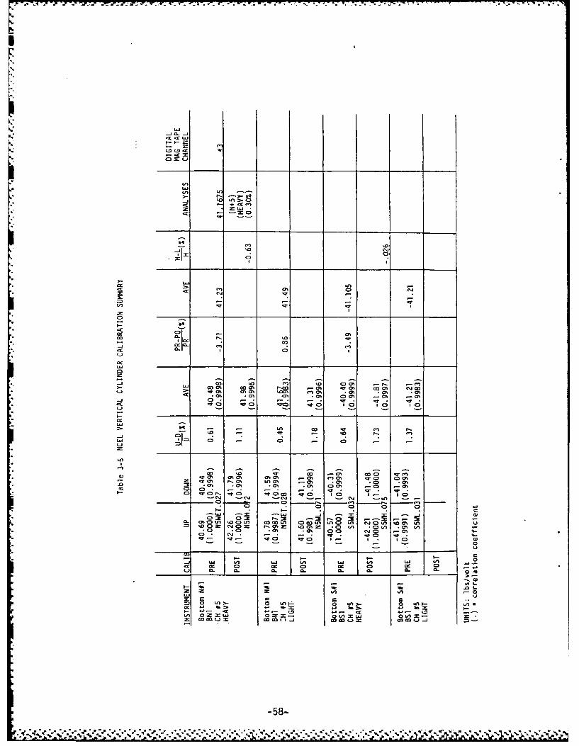
The results of the force calibrations are shown in Tables 3-3

through 3-10.

-17-

' '-. _.',".r,",.,-. .-. ,-'."-' "-"," .,,', . ... - . . .. . .. . .. . ....

The low range of calibrations are consistently steeper than the

high range of calibrations, but they only differ by less than 3.3%

for the instruments used in the analysis. The calibrations were

* quite linear and consistent. In summary, the force calibrations

were consistent, linear, and very repeatable between the beginning

of the tests and the end of the tests for all of the data channels

used in the NCEL data analyses. Table 3-4 shows that rEl Ch #3 was

not consistent and should not be used in future data analyses of the

transverse force and moments.

The cylinder was also calibrated at location 5 with the

cylinder in torsion. That is, the forces were applied to the edge

of the cylinder as shown in Fig. 3-24. This was done in both the

clockwise and counterclockwise directions. It was found that tor-

sional loads had very little effect on the output from the force

transducers. Therefore, if any torsional loads were applied to the

cylinder (and they could only have been so from uneven boundary

layer development between the east and west sides of the cylinder)

they would not influence the force measurements.

One calibration result for a pressure meter is shown in Fig. 3-

25. All of the amplified individual calibrations are available upon

request. They were all very linear except for P6 (the 2400

azimuth). Figure 3-26 is typical of the linear calibrations and

Fig. 3-27 shows P6. The calibration was made when the wave flume

was being filled or emptied. Some pressure meters had a consider-

ably larger calibration constant than others, but the calibration

values remained constant and the pressure measurements were consis-

-18-

. .. - - . . . . " - , . " . " . " . . ". . . .'.L..

.- . -- -

tent and reasonable for the measurements in waves. The pressure

calibrations are summarized in Tables 3-11 and 12.

The east current meter had been previously calibrated by Dibble

in (1980) at 20.77 fps/V, and after this testing by Kim in June 1983

at 20.47 fps/V (a 1.5% difference). A value of 20.6 fps/V was used

in the NCEL data analysis. This meter was more consistent than the

West meter and was the one used in the data analysis.

3.3.2 Test Plan

The test cylinder was designed and constructed in the Fall and

early Spring of 1982-83. Prior to assembly in the WRL, the force

dynamometers were bench tested to ascertain their workability. The

equipment was then completely assembled. Calibrations of force

transducers were made. The primary current meter (East side) had

been previously calibrated. The pressure transducers were cali-

brated as the wave flume was filled and emptied. The cylinder was

then subjected to 31 periodic waves to satisfy all requirements of

• the SOW, plus a few extra waves. Then four random wave sequences

were generated according to the SOW. Some time remained in that

work day so 10 more periodic wave runs were made at three wave

periods--to fall in between the. wave periods previously tested.

(However, only 26 periodic wave runs were processed, according to

the SOW).

The flume was then pumped down and calibrations were made for

the force transducers for comparison with the calibrations prior to

testing. The log of runs, Table 3-13, is self-explanatory, com-

pleting the description of the test plan.

-19-"wS.* .. * *. .*

Some photos of the cylinder subjected to the waves are given in

Figs. 3-28, 29 and 30.

* -20-

4.0 DATA ANALYSIS

Periodic wave data were collected on 22 April 1983 and the

random wave data on 25 April 1983. A total of 21 channels of elec-

tronic data signals were recorded during the NCEL tests. Table 4-1

identifies these 21 data signal channels and their method of record-

ing during both calibration and wave measurements. Only 16 channels

of analogue-to-digital (A/D) were available on the PDP-11/E1O used

at the WRL. These 16 channels are identified in the column titled

"AID Run Ch. #" in Table 4-1. the remaining five channels of data

recorded during wave tests were recorded on a Bell and Howell CPR-

4010 analogue tape deck and are identified in the column titled

"Analogue Tape Ch.#" in Table 4-1.

The local force transducers 9 and 10 were combined to A/D Cali-

bration Channel #9 as a single signal for both digital (A/D Run

channels #5 and #7) and in analogue (analogue channel #1) format

(see Fig. 3-20). A five-volt step signal was used to reference the

analogue time series to the discrete digital time sequence. This

five-volt step signal was sent by the PDP-11/E1O to the Bell and

Howell CPR-4010 analogue tape recorder at the instant digital

recording began. The local wave force transducer signal was

recorded simultaneously on two A/D channels in order to determine if

there was any significant phase shift introduced by the 8 Hz Rock-

land filters. The A/D Run channel #5 was filtered by the Rockland

filter while A/D Run channel #7 was not (see Table 4-1).

The data recorded on analogue tape were passed through the

Rockland two-pole Butterworth filters before recording. These

-21-

analogue data signals were again passed through the Rockland filters

before being digitized in order to filter out undesirable high fre-

quency noise introduced by the analogue tape recorder. The water

surface profiler was not filtered by the Rockland filter because of

signal distortions which are introduced into the record due to

"drop-outs" in the data. These distortions are characteristic of

all sonic sensors. The question of phase-locking the data properly

to the water surface then becomes important. All the data records

were filtered to produce the proper signal amplitudes and phase

angles with respect to the water surface. The theory behind these

filters is presented below.

Six channels of data were also recorded for immediate observa-

tions by a stripchart recorder. A sample record is shown in Fig.

4-1.

4.1 Record Format and Filtering

Figure 4-2 demonstrates schematically the data recording pro-

cedure for the horizontal current meter measurement.

A recorded measurement, m(t), can be expressed as a linear sum

of cosines and sines by

Nm(t) =a + Z (a cos2nf t + b sin2wf t) (4.1-la)

mo n1 in n mn n

N- H (f )exp(i2irf t) (4 1ib)

m n n

-22-

- .. - o . .- , • . . • . .

where m(t) is the raw (unfiltered) recorded value of the horizontal

current measurement, u(t), and amo = <m>, the average value of M(t)

during the recording interval. The Fourier transform of m(t) is

given by

MH(f) = m(t)exp(-i27rft)dt (4.1-2)

where the complex-valued Fourier coefficient, Hm(f), is defined as

H (f) = R (f) + im (f) (4.1-3a)m m m

or H (f) = IHm(f)lexp{ie(f)} (4.1-3b)

where the amplitude (modulus) is defined as

I (ffl = (R2+ 12)112 (4.1-4a)

and the phase by

0 m =TAN-I (4.1-4b)

Substituting Eq. 4.1-3b into Eq. 4.1-1b demonstrates that

am- R ( f), b = I (f). (4.1-5).m m m m

For example, high frequency noise can be filtered from a

measured signal, if desired, by setting a = bmn = 0 for f > fc

where fc is the "cutoff frequency." This type of digital filtering

will be termed the "FFr filter." High frequency FFT filtering was

done to many of the NCEL data records. For example, the high fre-

-23-

....................ov-..-..°. . . . . . .

- ~- --.

quency noise above 1.5 Hz was filtered from the horizontal current

and force measurements (see Fig. 4-10). That particular cutoff

frequency is specified on graphic plots when it was used. It was

selected arbitrarily to be low enough to sufficiently smooth the

signals, but high enough so that most influences from vortex

shedding would not be filtered.

When an operation is made on a signal from a filter, the

Fourier transforms of the signal and filter are multiplied in the

frequency domain in order to determine the Fourier transform of the

output from the filter. If the signal is passed through two

filters, as shown in Fig. 4-2, there are two multiplications. Thus,

the Fourier transform of the recording can be found from

Hm(f) = IHu(f)lexp{ieu(f)}IM(f)expfieM(f)}IHR(f)lexp{iBR(f) }

= IHm(f)lexp{iem(f)} (4.1-6)

where Hu is the transform of u, with phase eu (both quantities are

now sought); HM is the transform of the meter, which introduces the

phase shift, eM; and HR is the transform of the Rockland filter,

which introduces the phase shift, eR. lo simplify the following

discussion, it is assumed that IHR(f)I = 1.0 and OR(f) = 0. Later

the actual values can be considered and multiplied by the product of

the other two. Substituting hqs. 4.1-3a and 4.1-3b into Eq. 4.1-6

gives

Hm(f) = Rm(f) + i Im(f) (4.1-7a)

= Hu(f)[RM(f) + i IM(f)] (4.1-7b)

-24-

from which

Hum - m + ImM i ImMZ (4.1-8)

N+

The FFT filtered horizontal current u(t) is determined from the

inverse transform according to

L"O

u(t) = f H(f)exp(i2.ft)df (4.1-9)

Marsh-McBirney Filter

The single-pole filter characteristics of the Marsh-McBirney

current meter are

I'1(f) = I + i2wTf (4.1-10a)

2 -1[ [1 + (2wfT)2) * [1 - i 21fT) (4.1-10b)

where T is the time constant of the current meter and f is the

cyclic frequency of the signal in H.

The complex-valued FFT filtered signal, Hm(f), may be computed

from

I H mlexp(ie m ) m lHulexp(ieu)I HMlexp(ieM) (4.1-11)

which may be used to compute the amplitude of the current from

I Hm IIHl =T:V (4.1-12a)

and the phase from

eu : m - M (4.1-12b)

i - 2b-

The value of the time constant T is selectable on the Marsh-

McBirney current meters. One experimentally determined value for

the east meter was T = 0.159 sec. (see Fig. 3 and Table 4-1 in

Dibble, 1980). From Eq. 4.1-10b the modulus of the Marsh-McBirney

filter is

IHMI = [l+(27rTf) 2 ]" / 2 (4.1-13a)

and 6M = TAN- I{-2rTf} . (4.1-13b)

Table 4-2 summarizes the amplitude attenuation and phase shift in-

troduced by the Marsh-McBirney single pole filter in the NCEL data.

The current meters used have time constants, T, with three or

four selections. For the NCEL tests, they were set on 0.2. Small

differences in phase can make appreciable differences in Cd or Cm,

depending on whether the wave is drag or inertia dominant. The time

constants used for the NCEL data reduction were T = 0.159 sec. for

the east meter and T = 0.20 for the west meter.

Since the amplitudes in the frequency domain are proportional

to the amplitudes in the time domain, Eq. 4-13a also expresses the

division correction factor for the amplitudes of each frequency

component of the water velocity signal. Likewise, the phase angle

properly defines the phase of each signal. A problem was encoun-

tered with the horizontal signal from the west current meter. The

source of this problem has not been determined. However, the east

current meter (the same one calibrated by Dibble, 1980) gave excel-

lent results and is the one that was used for the NCEL data

analyses.

-26-

! . . .

Rockland Filter

The Rockland filter is a two-pole Butterworth filter. The

filter function is given by

f2 f2

HR(f - 0 0 (4.1-14)(i f) +20 1 fo i f+f (if)+2 foif+f0

where fo is the cutoff frequency, f is the signal frequency in Hz,

a1 = 0.924, and 82 = 0.700 for the flat decay response. Introducing

a dimensionless frequency ratio, e = f/fo, reduces Eq. 4-14 to

HR(F£) - 2 1+ i.848c 1 (4.1-15a)(1) )+i 1.848 (1-C )+i 1.4c

2 4 2HR(c) = (1-4.5872 C ft ) - i 3.248 (l"2 (4.1-15b)

(1-4.5872 2.+C) + 10.55 e2(1-22 )

The amplitude division factor, IHRI, is

IHRI = L(1+1.415 e2 c4 )(1-.04 2c4 )j-1/2 (4.1-16a)

and the phase angle, OR, is

eR3.248 =( -1 2 (4.1-16b)

R = TAN- (1-4.5872 £2 +c )

Table 4-3 summarizes the amplitude attenuation and the phase shift

introduced by the Rockland filters in the NCEL data.

Digital Formatting

Exactly ten periods of data were recorded for each of the 21

channels of data measured during the periodic wave tests. These

data were reduced to exactly eight waves and were digitized at a

-27-

;..

sampling interval determined by the deterministic wave period, T,

and the FFT base 211 = 2048 according to

At = 8T/2048 = T/256 (4.1-17)

Each single periodic wave in the eight-wave sequence thus contained

256 data values. This data digitization scheme was required in

order to insure that the data could be FFT filtered as previously

described using an FF[ algorithm of base 2. The FFT algorithm was

taken from Bloomfield (1976). Only seven of the eight waves were

actually used in the final data analyses.

The sonic profiler used to record the instantaneous water ele-

vation occasionally suffers from data "drop-outs" or "over-

ranges." These data are identified as "bad-points" and are removed

numerically by linearly interpolating between the good data

values. On rare occasions, these intervals of bad-points are ex-

cessively long and result in forming a fictitious wave (see Wave #4

in Run #5 in Fig. 4-5). These data have been ignored in the data

analyses because there were only two "bad point" waves in the total

of 182 waves recorded. These 256 data points per wave were reduced

to 33 data values (32 time increments) for each individual periodic

wave in the final data analyses for the force coefficients. The

total number of discrete data values digitized for the eight waves

in the 41 periodic runs that are identified in Table 3-13 was

-28-

.

NPTS = (41) runs * (21) channels (8) waves (256) ptsruns channe7 wave

= 1,763,328 pts

These data were FFT filtered to produce the records that were used

in the force coefficient analysis. The total number of discrete

data values used in the final force coefficient analyses was

NPTS = (26) runs (21) channels waves '33) ptsrun (7) channel (3 wave

- 126,126 pts.

For the four randomwave tests listed in Table 3-13, a total of

8192 data values were recorded during each test. The total number

of data values recorded during these random tests was

NPTS = (4) runs (21)channels (.192) Rtsrun channels

= 688,128 pts.

4.2 Data Processing

The 16 channels of digitally recorded data and the 5 channels

of analogue recorded data were all copied in digital format as inte-

ger values (0-4095) on magnetic tape by the PDP 11/E1O at the WRL.Iq

This data tape was then read by the CDC CYBER 73 main frame computer

at Oregon State University for subsequent data processing by a suite

of three FORTRAN-coded algorithms. Figure 4-3 illustrates schemat-

ically the flow chart for the data processing.

-29-

4.2.1 PROGRAM WAVE8

The integer data obtained from the POP li/E1O digitizing

process at the WRL was converted into physical units using the ap-

propriate calibration constants listed in Chapter 3. Figure 4-4

illustrates the calibration constants entered into the program for

run #5. Figure 4-5 illustrates a sample wave profile for run #5 in

integer (uncalibrated) values; and Fig. 4-6 illustrates the same

wave profile record following conversion from integer values to

physical units. Note the "bad point" values in the individual waves

#3 and #4. Figure 4-6 is also inverted compared to Fig. 4-5 because

larger integers (i.e., higher voltages) indicate wave trough values,

so a negative calibration constant is required (see Fig. 4-4, Column

#1: "WAVE PROFILE" -.5333).

Following calibration, the "bad points" were removed numerical-

ly by linear interpolation. On some rare occasions, the time

interval of "bad point" values was so long that these data were

interpreted by the numerical algorithm as an "inverted wave" and

were not removed by the subroutine. This rare event is illustrated

in Figs. 4-5 and 4-6 where the "bad points" in waves #3 and #4 have

not been removed; but have, instead, been converted to waves. This

rare event only occurred in the NCEL data during Runs #5 and #24.

Figure 4-7 illustrates the "bad point wave" in Run #24.

Figures 4-8 to 4-10 show the more typical results obtained fromthe "bad points" removed algorithm for Run #12. All1 of the wave

profiles recorded during the NCEL tests may be seen in Vol. II.

-30-

. " . .-

. . . .. . . . . . . . . . . . . . . . . . . .

. .. . . . . . . . . . ..,,* * . * .- * *il. . * . . .* * * * * * * *. . . * . .. * . . . . .

-r---r.. - -. R

Next, all data channels were Fourier analyzed by a FFT algo-

rithm with base 2. The FFT algorithm was written by Bloomfield

(1976). One-sided amplitude spectra were computed and visually

inspected for high frequency phenomena. The force amplitude spectra

were displayed graphically out to 10 Hz. Figure 4-11 illustrates a

transverse force amplitude spectra from the local force transducer

for Run #30. In order to obtain better visual resolution of the

spectral amplitudes at low trequency, all spectra were plotted out

to only 4 Hz. Figure 4-12 iI ,ustrates a sample horizontal current

amplitude spectrum for Run #5 at this expanded scale out to only 4

Hz. A digital, low-pass FF1 filter was then applied to the ampli-

tude spectra in the frequency domain to remove high frequency

noise. Inversion of the FF[ algorithm synthesized the filtered time

series for later analyses. Figure 4-13 illustrates a filtered time

series of the horizontal current for Run #5 with a cutoff frequency,

fc = 1.5 Hz. Figures 4-14 and 4-1b illustrate the effect of the

low-pass FFT filter on the bottom transverse force for Run #5.

Horizontal water particle accelerations required for the

Morison equation were computed from the measured horizontal current

by differentiation. Ihis differentiation was computed in the fre-

quency domain. Figure 4-16 illustrates a typical horizontal

acceleration amplitude spectrum computed from the measured data for

Run #5. Although the horizontal current amplitude spectrum had been

FFT filtered at 1.b H , Fig. 4-16 illustrates the problem of ampli-

fication of high frequency spectral amplitudes that is common in

numerical differentiation algorithms. In order to avoid this high

-31-

I. ,

" o " ' ' , , " o " , " ,t ' ' ' ' - " , . " , " , " , ° " ' . " . , " ° " . . . . .-- ".-•

frequency amplification, only the fundamental and the first harmonic

were used to synthesize the horizontal acceleration time series.

F igu re 4-17 illustrates the horizontal acceleration amplitude

spectrum used to synthesize a horizontal acceleration time series

from the measured horizontal current. Note that only the amplitudes

at the fundamental and the first harmonic have been retained and

that ALL of the other amplitudes have been set equal to zero.

Figure 4-18 illustrates the horizontal acceleration time series

synthesized from the amplitude spectrum shown in Fig. 4-17.

4.2.2 PROGRAM FDATA5/FD5A

The FFT filtered data from PROGRAM WAVE8 were read into PROGRAM

FDATA5 or FD5A for the selection of seven individual periodic waves

from the continuous eight wave sequence.

PROGRAM FD5A automatically selects the first seven waves in the

sequence beginning with the first crest as showen in Fig. 4-19. The

period of each individual wave in the seven-wave sequence is deter-

mined by first establishing a time at a wave crest, e.g. crest

number; secondly by adding one wave period to (as set into the func-

tion generator that drives the wave board) that time. This accounts

for the small variability in wave periods found in the data analyses

tables in Section 5. However, the small error involved averages to

zero. The wave heights are computed by averaging the leading and

trailing crest elevations and then subtracting the trough value in-

between the crests.

PROGRAM FDATA5 allows for the manual selection of the individ-

ual waves shown in Fig. 4-20. Cross-hair cursors on the TEKTRONIX

-32-

I, .-.I . * . . . . ..•

4010 screen are positioned at the individual wave crests and troughs

to define the seven individual waves. The wave heights and periods

are then computed the same as in FD5A. Figure 4-21 illustrates the

* manual determination of the individual waves by PROGRAM FDATA5 for

Run #5. Only Runs #5 & #24 were processed by PROGRAM FDATA5 in

order to manually override the automatic selection of the fictitious

- "bad point waves" that would have occurred had PROGRAM FD5A been

used.

Finally, both programs reduce the number of data values in an

individual wave from approximately 256 values (= 2048/8) to 33

points per wave (32 time increments). This reduces the CPU time

required to compute the force coefficients, Cd and Cm, by Fourier

analysis without loss of accuracy.

4.2.3 PROGRAM LABT4

PROGRAM LABT4 computes force coefficients, Cd and Cm, from the

two-term MOJS equation by least-squares analysis. Each of the seven

individual waves selected either automatically from PROGRAM FD5A or

manually from PROGRAM FDATA5 is analyzed separately. First, an

average velocity is computed from the measured horizontal current

profile. Then the drag, Cd, and inertia, Cm coefficients are com-

puted by least-squares analysis according to Sarpkaya and Isaacson

(1981). he predicted 2-term Morison equation force is given by

F (e) = 1/2 CdPD[u(e) + <u>]Iu(e) + <u>1 + 1/4CmPTD 2 ;(e) (4.2-1)

-33-

....................................................

. _ ~~. V__. . ..

where Fp(o) is the instantaneous predicted local in-line force per

unit of the vertical cylinder and <u> is the average velocity. A

mean-square error between the instantaneous measured force per unit

length, Fm(O), and the force predicted by the 2-term Morison equa-

tion in Eq. 4.2-1 may be defined by

2 1 27t 22- f [F (e) F (6)] do (4.2-2)

The drag, Cd, and inertia, Cm, coefficients may be estimated from

4.2-2 in a best least-squares sense according to

"2 2.. 0C a E 0 (4.2-3)

d m

By Cramer's rule, the estimates for the two force coefficients are

given by

BI1A 4 - B 2A 2C = 1 4 2(4.2- 3a)m 1/4 prD DET{Cm , Cd}4

B2A1 - BA 2

C ~2 1 12 (.-bCd = 1/2 pD DET{Cm , Cd} (4.2-3b)

where

n2

A1 f u2 (a )do027

A2 = f u(O)[u(o) + <u>]Iu(o) + <u>Ide0

A4 f 2 [u(6) + <u>]4 do02r

B1 0 f Fm(o )u(o )d(o)

-34-

e..p ° ..- , m " ° . o , . .... .°, , ,. . . . . . . . . . . . .-. . . . ..

2wB2 = f Fm () Eu(e) + <u>Jlu(e) + <u>lde

DETC m, Cd } = A1A4 - A2 (4.2-4)

The integrals in Eqs. 4.2-4 were evaluated numerically using

Simpson's rule (Crandall, p. 161, 1956).

The horizontal water particle kinematics required in the inte-

grals in Eqs. 4.2-4 were computed by three different means: 1) by

the measured kinematics from the east current meter; 2) by the

linear wave theory plus the average measured velocity; and 3) by the

nonlinear Dean stream function wave theory plus the average measured

velocity. In addition to the three sets of water particle kine-

matics used to obtain the force coefficients, two additional sets of

existing force coefficients were employed in the analysis: 1) Wave

Project II coefficients; and 2) U-tube coefficients. Both the root-

mean-square and the maximum errors between the measured and

predicted forces were computed for each of the 7 waves analyzed for

each Run.

The Wave Project II force coefficients were computed by

C = 1.33 (4.2-5a)

1.20 ; R < 2.0xi0 5

Cd(-) = 0E ; 2.0x10 5 r R 4 5.5xi06 (4.2-5b)

0.55 ; R > 5.5x106

where

E = 3.59197- 1.02271og1 0 (R) + 0.0673774[1og1 0 (R)] 2

-35-

S .... , _ ,.. . . . --% . . -- . . . , ", -.. -,. . 1.* a -, rt . -- •.2".-,-,

R = Iu(6) + <u>1/v

and where R is the instantaneous Reynolds number and v : kinematic

viscosity of the fluid (= 1.41x10 5 ft2/sec.). Since Cd varies with

R (and time, or e), there is no single value to show for a

particular run. The maximum Reynolds number possible during any run

is 3x10 5. Therefore, according to Eq. 4.2-5b, the drag coefficient

will vary as 1.03 < Cd 4 1.20.

The U-tube coefficients published by Sarpkaya and Isaacson

(1981) do not extend to either the Reynolds numbers or the Beta

values measured for the NCEL data. Since U-tube tests have never

been extended to the Reynolds numbers or to the Beta values obtained

in large wave tank experiments, it is questionable that the U-tube

values can be reliably extended to in-service design of prototype

structures. Nevertheless, an effort was made to extrapolate

graphically the data reported for U-tube tests. The results ob-

tained by these graphical extrapolation methods are not unique and

should not be interpreted as recommendations for the use of U-tube

coefficients for computing wave forces. They were done for interest

only in accordance with the SOW.

The U-tube inertia coefficients were estimated from

(2.00 ; K < 2.0

C = 0.001336K - 0.029881K 2+ 0.17002K + 1.71668 2.0 K 11.0

1.75 ; K > 11.0 (.2-6)

The U-tube drag coefficients were estimated from

-36-

I.•

-... . -, -...... -...-...-....- -.... ,,..-.-..-. ..-..-.. '..'....2,...':."2...--.,.-...-.....-.,.-,.. '-.'....,. ...-. . . -..... .-

!..'-.-:-',.- .. /..' , ,.- - -.- , . . . . . . . . . ,,m .J,,m.. ,m. . -. . ,,, . . . . . . . .. lm

R < l.Ox105:

Cd = 0.000476K3 - 0.017877K2 + 0.185404K 0.244354 (4.2-7)

* R > 1.Ox1O5:

r0.5 ; K < 2.5

I3 2Cd 0.00124K - 0.3636K + 0.280324K- 0.000779 (4.2-8)

L 0.55 ; K > 8.0

Measured Kinematics. Figure 4-22 illustrates the measured

horizontal water particle kinematics and the numerically computed

horizontal water particle acceleration for wave #3 in Run #5. The

measured horizontal water particle velocity includes the average

current, <u>. The units of the vertical axis in Fig. 4-22 are ft.

for the water surface elevation, ft/sec for the velocity and ft/sec2

for the acceleration. Figures 4-23 to 4-25 compare both the

measured forces and the forces predicted by the 2-term MOJS equation

using the measured horizontal water particle kinematics and each of

the three sets of force coefficients.

Linear Wave Theory Kinematics. Figure 4-26 illustrates the

horizontal water particle velocity and acceleration computed from

linear wave theory for wave #3 in Run #5. Figures 4-27 to 4-29

compare both the measured forces and the forces predicted by the 2-

term MOJS equation using the linear wave theory kinematics and each

of the three sets of coefficients for wave #3 in Run #5.

Table 4-4 summarizes the three sets of force coefficients (Cd

and Cm) that were used individually with each of the three different

-37-

'p

" " -,.". " '-'-';.'-..- - - -. ' ''....'''.-'* '- ..- --. . - . -.-. .-.-. '- -'..' ,' .. -. .... ".. . - . . . .-..

wave field kinematics. This resulted in nine different analyses for

each of the seven individual waves in each of the deterministic runs

listed in Table 3-1 that were analyzed by the 2-term MOJS

equation. (In addition, the 4-term MOJS equation was used with the

three sets of kinematics, yielding a total of 12 different analy-

ses.)

Stream Function Theory Kinematics. Figure 4-30 illustrates the

horizontal water particle kinematics computed by the stream function

wave theory for wave #3 in Run #5. Figures 4-31 to 4-33 compare

with the measured forces and the forces predicted by the 2-term MOJS

equation using the stream function theory kinematics and each of the

three sets of coefficients for wave #3 in Run #5.

Four-Term MOJS Equation. The 4-term MOJS equation developed by

Sarpkaya (1981) introduced two additional time-dependent terms

having universal coefficients that could be used with the Fourier

coefficients obtained from the 2-term MOJS equation (Sarpkaya, 1981,

p. 59). Since these universal coefficients were developed by

Sarpkaya (1981) specifically for the use with the Fourier coeffi-

cients obtained from the 2-term MOJS equation, it was not realistic

to use either the Wave Project II or the U-tube force coefficients

in the 4-term MOJS equation since they were not obtained by Fourier

analysis from the NCEL data. Consequently, only the least-squares

coefficients were used for each of the three sets of wave field4,

kinematics in the analysis by the 4-term MOJS equation. Sarpkaya

and Isaacson (1981) have shown that the inertia coefficients are

identical between the Fourier and least-squares regression analyses

-38-

i- -'''"-" '- - " -" .-

°--"- '- - -. -" - - - - - - - - -.. -- - -.. ° _.: " . . . . . • , . . - .

and that the drag coefficients differ only slightly (Sarpkaya and

Isaacson, 1981, p. 90). Therefore, the least-squares force coeffi-

cients were used with the universal constants in the 4-term MOJS

equation in the NCEL data analyses.

Only the least-squares coefficients were used to compute the

predicted forces by the 4-term MOJS equation using each of the three

sets of kinematics. Because some of the inertia coefficients com-

puted by Eq. 4.2-3a were greater than 2.0 and some of the drag

coefficients computed by Eq. 4.2-3b were negative, the lambda term

in Eq 2.1-2 sometimes becomes negative. When this occurred the two

additional terms in the 4-term MOJS equation were not used.

However, if the inertia coefficient was greater than 2.0 and the

drag coefficient was less than zero, then lambda was positive and

all four terms were computed.

Figures 4-34 to 4-36 compare the measured and predicted forces

computed by the 4-term MOJS equation for each of the three sets of

kinematics using only the least-squares coefficients for wave #3 in

Run #5.

4.3 Random Waves

Four random wave runs were recorded during the NCEL tests. Two

of these four random wave runs were analyzed and 10 individual

periodic waves were selected for analyses based on comparisons with

wave heights and periods in Table 3-13. A suite of three computer

programs was developed to analyze the 10 individual periodic waves

that are listed in Table 4-5.

-39-

"., -, "- ",-. .. '-,. .,*"%* f*.~ qr qw - .. -:,.. - ... o- , , - . . -. o,.- .- .._ - ,,.- *-%.*. , . ,.,.- . . -*.- %., ''-, ,a--

4.3.1 PROGRAM WAVER

PROGRAM WAVER calibrated the integer data from the random wave

runs similar to PROGRAM WAVE8 for the deterministic wave runs. A

block of data containing 512 values was considered as a sequence of

periodic waves. The fundamental wave period was then determined

from T = 0.06*512 = 30.72 sec., where at = 0.06 sec. This single

block of data was then FFT filtered to remove the high frequency

noise. The time series for the horizontal water particle accelera-

tion was computed numerically as before for the deterministic wave

data in the frequency domain. However, there seemed to be a little

more high frequency noise in the velocity spectra for the random

waves. Thus, the high frequency noise problem in the acceleration

spectra were exacerbated due to the transfer function approach that

was taken. In order to obtain relatively smooth and useful

accelerations, the acceleration spectra were generally filtered at

0.5 Hz instead of 1.5 Hz, which was the general case for the

velocity spectra. There was one exception for Run 32, wave #2,

where the horizontal acceleration was filtered at 0.4 Hz.

4.3.2 PROGRAM FOATAR

The FFT filtered data from PROGRAM WAVER were then visually

inspected on the TEKTRONIX 4010 CRT screen one block at a time.

From the hard copy output, the individual waves were selected on the

basis of wave height and wave period. Figure 4-37 illustrates a

single block of 512 values of the wave profile from random wave

#32. The individual wave #6 was selected for analysis as an indi-

vidual periodic wave. The number of data values in the individual

-40-

".'%"" .'" ' 9.:. "" ' i' % ' F " - ' ' i

.- -n , , . " , . T. -"",%o' .. 'i' '. ,' ..- --. < , , , - • . .- 5.-I i* iIN"'.~

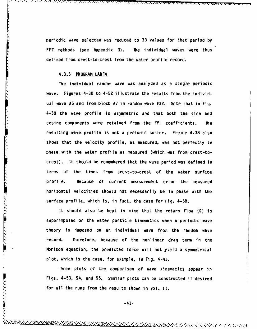
periodic wave selected was reduced to 33 values for that period by

FFT methods (see Appendix 3). The individual waves were thus

defined from crest-to-crest from the water profile record.

4.3.3 PROGRAM LABT4

The individual random wave was analyzed as a single periodic

wave. Figures 4-38 to 4-52 illustrate the results from the individ-

ual wave #6 and from block #7 in random wave #32. Note that in Fig.

4-38 the wave profile is asymmetric and that both the sine and

cosine components were retained from the FF1 coefficients. [he

resulting wave profile is not a periodic cosine. Figure 4-38 also

shows that the velocity profile, as measured, was not perfectly in

phase with the water profile as measured (which was from crest-to-

crest). It should be remembered that the wave period was defined in

terms of the times from crest-to-crest of the water surface

profile. Because of current measurement error the measured

horizontal velocities should not necessarily be in phase with the

surface profile, which is, in fact, the case for Hig. 4-38.

It should also be kept in mind that the return flow (0) is

superimposed on the water particle kinematics when a periodic wave

theory is imposed on an individual wave from the random wave

record. Therefore, because of the nonlinear drag term in the

Morison equation, the predicted force will not yield a symmetrical

plot, which is the case, for example, in Fig. 4-43.

Three plots of the comparison of wave kinematics appear in

Figs. 4-53, 54, and 55. Similar plots can be constructed if desired

for all the runs from the results shown in Vol. II.

-41-

;- ' : ; :n 3; * *-,-. ;. .. * * ............. . ....

5.0 SUMMARY OF RESULTS

Table 5-1 summarizes the average force coefficients from the 26

periodic runs. Table 5-2 summarizes the force coefficients from the

seven individual waves for each of the 26 periodic wave runs and

then the random waves. Each of the seven individual waves were

represented by 33 data points from the original 256 data points.

The two "bad points" waves in Runs #5 and #24 are identified by

asterisks.

Figures 5-1 to 5-3 illustrate the parametric dependency of the

average inertia force coefficient, Cm, on the Keulegan-Carpenter

number, K, for the 26 periodic waves. Figures 5-4 to 5-6 illustrate

the parametric dependency of the average drag force coefficient, Cd,

on the Keulegan-Carpenter number. Note that negative drag coeffi-

cients are not plotted. Also shown in Figs. 5-1 to 5-6 are the

maximum a values obtained from published U-tube tests (Sarpkaya and

Isaacson, 1981) and the 0 values for these tests.

*- Figures 5-7 to 5-9 illustrate the inertia force coefficients

for the 10 individual waves selected from the two random wave

runs. Figures 5-10 to 5-12 illustrate the drag force coefficients

for the 10 individual waves selected from the two random wave

runs. Again, negative values of Cd were not plotted.

Table 5-3 summarizes the RMS error and the absolute value of

the maximum error for both the 26 periodic wave runs and the 10

individual waves from the two random wave runs. The RMS errors were

calculated from the differences between the predicted force and the

measured force (as functions of time). In each case the predicted

-43-

force was based on the choice of kinematics and coefficients as so

indicated. For example, under the stream function theory and WPII

columns, the stream function kinematics, in conjunction with the

force transfer coefficients as obtained from the WPII data, were

used.

Table 5-4 summarizes the RMS error as a percentage of the maxi-

mum force for the 26 periodic wave runs and the 10 individual waves

from the two random wave runs. Also tabulated is the percentage of

energy in the two-harmonic acceleration spectrum compared to the

unfiltered acceleration spectrum. This measure indicates the loss

of energy in the acceleration spectrum due to filtering the non-

harmonic components in the spectrum. Figures 5-13 to 5-21 display

the RMS error as a percentage of the maximum force for the range of

Keulegan-Carpenter numbers measured. These results were obtained

from the 2-term MOJS equation.

Figures 5-22 to 5-24 display the RMS errors as a percentage of

the maximum force for the range of Keulagan-Carpenter numbers

measured for the 4-term MOJS equation. Table 5-5 summarizes the RMS

errors for the analyses dealing with the 4-term MOJS equation.

-44-

. .. . . . . .. - . - ._*-..-*- :,',' . .. , , ,, * ." ,.. : .,::.'' .

6.0 CONCLUSIONS

-. Data of high quality were obtained on measured forces and wave

conditions for a 12.75-inch diameter vertical cylinder. Drag

and inertia coefficients were obtained therefrom for wave con-

ditions with a Keulegan-Carpenter number up to 16 at the local

force transducer and 20 at the still water surface. According

to the open literature, this environment should have produced

conditions that were drag dominant (although the inertia

effects should still be significant). However, the results

indicate the conditions were inertia dominant (and the drag

effects were still significant).

The assumption that drag-dominated wave forces exist at

Keulegan-Carpenter numbers near approximately 20 is not cor-

rect. This assumption arises from U-tube results which

demonstrate that there is no parametric dependency of the force

coefficients for K > 20. In contrast, the Dean number, E, (see

Appendix 11.2) demonstrates that wave data do not become inde-

pendent of K until E ) 4.0, and E .088 K, from which K

45. As a consequence, most laboratory data determined herein

are dependent on both Cd and Cm. For the data with K s 6 we

found that the center forces were completely inertia dominated.

2. lhe wave forces as functions of time were calculated using

measured kinematics and theoretical kinematics from linear and

stream function theory, using least square coefficients, Wave

Project II coefficients, and U-tube coefficients--all for the

-45-

F .. .. . ' i . - _ . . . . . . . .. ... • -, .- r -" " *" - . . . . ." " ' '" "

2-term MOJS equation; and for the 4-term MOJS equation using

least square coefficients. The a values were much higher than

normally seen for laboratory testing. In fact, they were only

moderately smaller than for conditions at sea. 1he Cm values

for measured kinematics were slightly larger than for the

linear and stream function kinematics. The Cd values for the

measured kinematics had less scatter than for the two theoreti-

cal kinematic models. In addition, the values of Cd in the

range of K where they were relatively reliable (K > 10) were

approximately one-half those reported by Sarpkaya (1981) for

oscillatory flow U-tube experiments with 8 values up to 8370.

3. Plots of the RMS errors vs. K indicate that the most accurate

analysis methods used herein were the measured kinematics and

the coefficients derived from a least square analysis.

4. he published U-tube coefficients do not extend to high enough

Reynolds numbers or beta parameters to be used for the OSU

laboratory wave analyses. Since the Reynolds numbers and beta

parameters in the NCEL-OSU laboratory wave tests are still

lower than in-service ocean designed values, U-tube coeffi-

cients, should be viewed with caution for wave force design.

5. The 2-term MOJS equation gave lower RMS and maximum errors than

did the 4-term MUJS equation. he universal coefficients in

the 4-term MOJS equation were not valid for these laboratory

wave data.

-

i -46-

S a

6. The 2-term MOJS equation used with measured kinematics and

measured coefficients gave lower RMS and maximum errors com-

pared to either linear wave or stream function wave theory

kinematics or the Wave Project II or U-tube coefficients.

7. Linear wave theory and stream function wave theory kinematics

should be corrected for wave tank circulation currents in wave

force analyses.

8. Although interesting observations have been made from the

several types of calculations required by the SOW, many other

analyses wait to be made on the data. Some of these are:

a) Phase shift vs. K plots for water surface vs. total

force.

b) Maximum force coefficient vs. K plots.

- c) In conjunction with a and b, new Cd's and Cm's can

be derived.

d) Total forces and overturning moments can be exam-

ined.

e) Transverse forces should be examined regarding maxi-

mum litt coetticients.

f) More analyses should be directed to the random wave

runs. Much more extensive transfer function and

wave-by-wave analyses can be made to shed light on

proper methods and techniques that differentiate

analyses in random waves from those for periodic

waves.

-47-

g) For both periodic waves and random waves a cross-

correlation analysis may produce more insight to the

phase shift model.

9. The phase shift and maximum force coefficients analysis

referred to above has innate advantages. First, both the phase

shift and maximum force coefficient are nore stable, displaying

little scatter for all values of K. Secondly, the relative

importance of the drag or inertia term is immediately evident

in the phase plot. lhirdly, the maximum force is much more

accurately predicted than in any of the methods utilized in

this work. It should be added that this proposed technique has

only recently revealed itself. In fact the ideas encompassing

the new methods were stimulated by this research. lhey should

be further explored because of the promise of a major improve-

ment in available methods of determining Cd and Cm from labora-mI

tory experimentation and projecting the results to prototype

conditions.

-48-

:- 'Z.-.- .- '--. .. .,'-. - '- -... '-... ...................-.............. ..

7.0 REFERENCES

Bloomfield, P. (1976), Fourier Analysis of Time Series: An Intro-

duction, Wiley-Interscience, New York, NY, pp 75-76.

Crandall, S.H. (1956), Engineering Analysis, McGraw-Hill Book Co.,

NY.

Dean, R.G. and P.M. Aagaard (1970), "Wave Forces: Data Analysis of

Engineering Calculation Method," Journal Petroleum Technology,

March, pp 368-375.

Dibble, T.L. (1980), "Frequency Response Characterization of Current

Meters," thesis submitted in partial fulfillment of the re-

quirements for M.S.C.E., Oregon State University, Corvallis,

OR.

Hudspeth, R.T., R.A. Dalrymple and G. Dean (1974), "Comparison of

Wave Forces Computed by Linear and Stream Function Methods,"

Proceedings Sixth Offshore Technology Conference, OTC Paper

2037, Vol. II, pp 17-32.

Sarpkaya, T. (1981), "Morison's Equation and the Wave Forces on

Offshore Structures," Naval Civil Engineering Laboratory Report

CR82.008.

Sarpkaya, T. and M. Isaacson (1981), Mechanics of Wave Forces on

Offshore Structures, Van Nostrand Reinhold Co., NY.

-49-

8.0 ACKNOWLEDGEMENTS

The authors wish to thank Mr. Jerry Dummer of the Naval Civil

Engineering Laboratory for his support and encouragement during this

project. In addition, Mr. Charles Smith of Minerals Management

Service provided additional support that allowed for a more complete

analysis. The computer programs, data acquisition, and analyses

were helped greatly by the efforts of Mr. David Standley and Mr.

Ming-Kuang Hsu. The laboratory work was conducted by Mr. Larry

Crawford.

-51-

9.0 TABLES

-53-

Table 3-1 Measurements of LFT surface alignment. OUT from the cylindersurface = +, IN = -. Bearing means 00 = North (downwave)1800 = South (upwave) and 900 = East. Measurements in mm.

Bearing Bottom Top Longitudinal Spacing(degree) Alignment Alignment From Cylinder

Top Bottom

0 0.0 + .8 1.4 1.5

30 + .3 + 1.1

60 + .4 + .8

90 + .5 + .4 1.5 1.9

120 + .5 + .2

150 + .3 0.0

180 + .7 0.0 1.5 1.3

210 + 1.0 + 1.0

240 + .8 + .9

270 + .5 + .3 1.5 1.0

300 - .6 - .5

330 - 1.1 - .5

Average + .3 + .4 1.5 1.4o .6 .6

-54-I i: ... .-.. .. . . . . . ..- " " ""-'- -'- " '- " " "'" '" "- "' " " -'"" "" '"- "'- '""""

Table 3-2 Light and heavy calibration weights

Calibration Weight (Ibs)

Step Light Heavy

1 0 0

2 .74 3.22

3 2.66 14.35

4 4.59 28.07

5 6.54 43.45

6 8.50 63.92

7 10.47 84.46

8 12.47 108.33

9 14.51 132.64

10 16.56 157.08

11 181.61

12 201.44

S.

.4.

.

-T -

4 -CL

LuJ

in C

Lu iO

tntCD

CD 0. -0 I

C-3

wu L" CD. (N0 m ~ 0l ON 0CD at 0D% aC3 r CD 0 (% (3 ' 0 0 9 1, 1 a,% 0% 4m0 (

Z -90 0 a! % o .G! *0! .% .

(N. nJ n *

CD 0 40 0

01 . -9 .

0. 0 D Z~ OD ( 0 (3 CD % D M MI 0a

C-)

Lj CL I. 0.m C. L

0iJ .l .l u

'a- -- CO- C-4 0- .- 0%-

CL~ CLJ r*. N0% a0 00 nO 0M .0 M0 *0% *D m0 *

-0 u 0 i . (i '.* i. 5 . '

- ~ -56-

- I-. I-A%

La

%n

L~Le

U

0n

=I- ~ ~ 0%% m h 0 h % -

In 0oL

La

0% Ch Ch 'n0P,0%l~ ~ a 0 00% 00% - Cn0 it0 at % 0

P. 4 n 100 M00 IV % Ow0 h 0 aZ~ ( 0% '% .0 . m .0 m

q- 01 q - r .

-J - 0wC -0 0 - -' W -

Li110 0- - 1-. *- CA 0o Ius w .

0c 0 0c C wa

L Z ,

CK Z. "t .- b .

0 0 *i - 0 . . * N j . ~

Ga ~N ~ 0 ~ ~0 0% a0C. ~-57-

LaJ-i u-

OZ )

* Lu

I-. .. Cl

-=0

00

0.1

C)-

Li L

a! C

-J~~L CO '0' 0 --. .r

La o C0% a, C q* 0 co - 0% co~l CC.) ~ ~ ( 0%0 I0% Oll L 0 0 0

m~.0 .0% 0:% M% 00% -0%

Ma 0 -: a I a .- I

'o0%n 010% t LO0 U!0 -0 t 0 0 W$.D0 x0 .0c m C " .0% V00, . 0 .qa -01

0 0L CL. m

= 0 to .0% .0n F--JO > .- 0%l

- I- .-. 9--5--

(30. -J

4= AJ

-j -J

0% C"C CW % F m a% qc

dc .m0 "0% w

Lfli

I- L

L" 0 7 5 m 0 m k 0% 0

L.Au0o - -f - --

00% 1 r0 at.0 00% .at C4. Q0% .0%W . * r, at coo . .* A

L.40

@0 Al n i 4 @0w 0 cz a

ti Q. 0 0 a. C0 0@00

0~ *j 0 )a - * 4.j C2 ca 4.1'

cc uam -)

0.~Q~0Q Z -59-ZA0 Z~8 n(J i 0 f

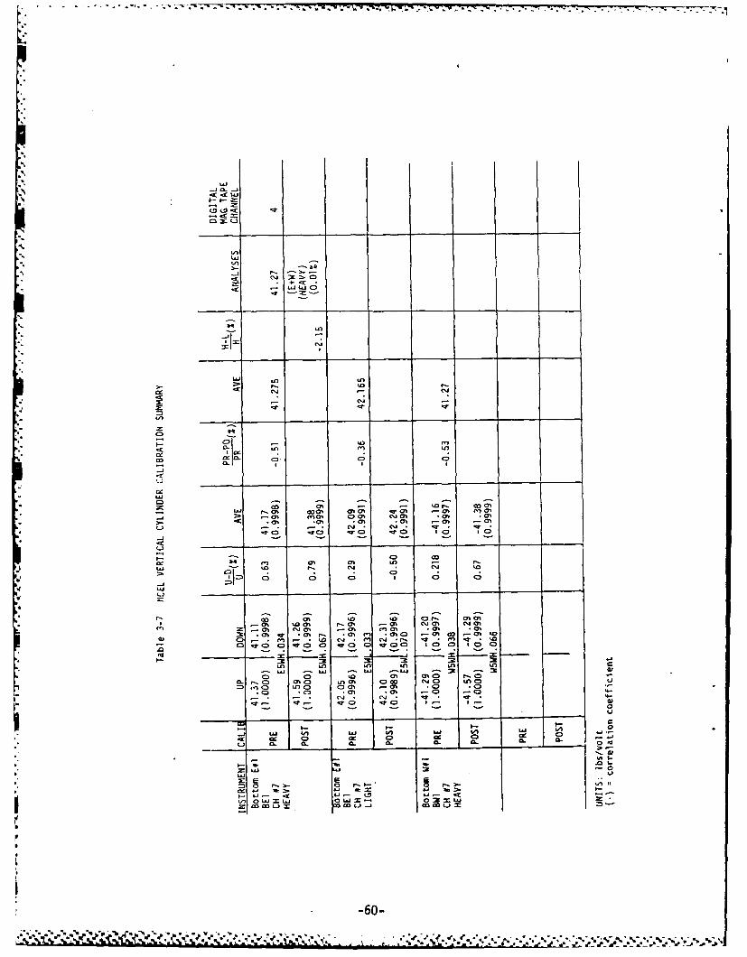
.CC3 o

m Ln

U)

U)I

cez~.W JU

("I "I"'

x' -m o

k-3I

I 0 ON00O

-A 0-S In _n n L

ZCO C, -0 m lO CDO

-- 0 ON CPlO 06) C 0 c-4 a 0)C .) (D C 0) .6 0%) -

(.3 - r Q

L., w) P. C 4i VI

WJ 0 0 0 0 .

cL C

r-.j C" Z9 t) U P. 60

0 1"0s00 ~ s0 00 .

'U 60-

ujV-j CL -

c Lu 4.-CJ

L~a L~J0.t 4h

4IA -

LAWS

C; 40

-JA W) - I%0

o. 0

LAS-

M.1 at a t 0 % In % h

0~ 04

00 -TC IC nO

CDo -j I ~ - - -

4m 'm V) 4A 0% I'a % 0 w- (-~0% a% % 0 0% 0u U1 %

CL c 43% 4m -0 (-O %00% ON ('0 '00! .0% co0% en % *09 I"! 00% 4M n

LiL

L~~~4 - ..0

1~~~3 0 u-j+cm+J

Ot 0% 0% 0% 0% 0 04 0

CX +% +% 0 %0 % 0(.0w (D0 + - "I0 - % 0% 11% %% %

00% uI T0% _.0 _j0 U 10 _j' _0% _jqq_0_

ce L4J

no C

L

inn

-- J

cc iL" CD>. C~j C

cna'a 'a8;7 an

0cC

Lo C0 3 C

0LnuI u

C3 t

CDO co C7

m "aa

J.0 .0co>L)"

M-.0 co0 .o01-ic

0 .01 t -62-

bA

An

U.'

kn n

-Jl

In ____ --

o T o

to- at

en 2K

C31 -; m

0a 0 %

j cn F, _j I.

LAc

-63

.,c . LLu

Inn

-i cu

oo co 0%%a GL- Gol In -04 %

.- 0D 4

0j 0

-AJ - -

Go

-wJV -- A . P % %c - o

0% 4m -. c

c2 Is - -w'

JU i c'j f" ~ . 0 003 Go co GO f" 0 0

-I - c

o, r o 0~ nm mV ; c 0 f ". c1d oea fl cm 0% 04 I0 Qcjq m cj- 7 3 r n

LA.D 00

010 im. c U0 9100 Coll . cn0 i

CD (ML" 0 04

.0 - ' -64-

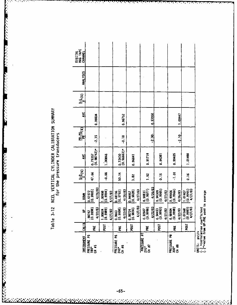
F . .

-' ". . '- ... . --u ., . . . . -. . . , , , ma,

a! a. -

coi

(n

CA

b-J

- c

- en 0 r m d P

% e o 'o a, g t t m 4 V P

i,- at - t r ! x ! r. a ! ' %1-w cm w a,,,,,a 4

It a % 0% aa

'.S,_ S.. -" "- ,',

;-, o- I,, ! .,,. " -I o •' I" •oa m - % a t .. i_ 0-.

-. u- 4 --

050 % - nvl. (A -' -m v)

o" .La cc w 0

"...,. *0 * .0

- 4w d L 0l cc 0

'-a . I ).,., - 0

,%% P ' 0 .. " ' % 050% "r 5 * . .

Li 0 .% cm

.- 65-

z - * %" -0 "' ' """ "% " % %" " %""""" *" "°

"% "e 'm', "'~~~~-" 0- 0-" ' 0- q" 0-" ''' "- - ' "a C '" -

Table 3-13 Log of runs

I Wave Target Analog Counter

Run No. Frequency T Span H Start Stop RemarksS(lz) (s) (waveboard) (ft)

1 .500 2 95 1.0 35 512 .500 2 32 0.4 51 653 .400 2.5 110 1.1 66 83 X 10 A/D - 24 .400 2.5 205 2.0 83 101 X 10 - 25 .400 2.5 375 3.7 101 119 X 106 .270 3.7 175 1.0 119 140 X 10 -7 .270 3.7 444 2.5 140 163 X 108 .270 3.7 780 4.4 163 185 (voltage out of r9 .217 4.6 147 0.7 185 209 X 1010 .217 4.6 336 1.6 209 233 X 1011 .217 4.6 827 3.1 233 257 X 10 - #212 .217 4.6 1000 4.3 257 281 X 1 - #213 .189 5.3 202 0.9 281 308 X 1014 .189 5.3 338 1.5 308 334 X 1015 .189 5.3 693 2.6 334 359 X 1016 .189 5.3 933 3.5 359 386 x 117 .189 5.3 1000 3.9 386 412 X 118 .167 6.0 665 1.9 412 445 X 10 4/25/8319 .167 6.0 800 2.6 445 477 X 1020 .167 6.0 950 3.3 477 510 X 121 .238 4.2 1000 5.2 510 537 X 122 .189 5.3 1000 3.9 537 568 X 123 .217 4.6 1000 4.3 568 597 X 124 .270 3.7 780 4.4 597 622 X I25 .400 2.5 375 3.7 622 645 X I26 .167 6.0 950 3.3 645 676 X 127 .5 2 95 1.0 676 698 X 10 Copy of R128 .270 3.7 780 4.4 698 723 X I Copy of R829 .217 4.6 827 3.1 723 751 X I Copy of RII30 .167 6.0 665 1.9 751 784 X I Copy of RIB31 .67 6.0 800 2.6 784 816 X 1 Copy of R19

32 Random JONSWAP I 3.7x Hi/ 3 1 2.9 816 990 X 1

33 Random JONSWAP T = 3.7x HI/3 -2.9 990 1160 X 1

34 Random JONSWAP T - 3 .7x HI/ 3 =2.9 1160 1330 Different

35 Random JONSWAP = 3.7x HI/ 3 =2.9 1330 1498 X 1

36 .333 3.0 140 1.0 1498 1519 X I37 .333 3.0 320 2.5 1519 1539 X 138 .333 3.0 850 5.0 1539 1564 X 139 .250 4.0 180 1.0 1564 1587 X I40 .250 4.0 450 2.5 1587 1610 X 141 .250 4.0 900 5.0 1610 1633 X 142 .200 5.0 200 1.0 1633 1660 x 143 .200 5.0 700 2.5 1660 1684 X 144 .200 5.0 1000 5.0 1684 1710 X 145 .333 3.0 650 5.0 1710 1731 X 1

NOTES: Water Temperature - 50F (4/22 8 4/23)Water Depth -11.5 ft.

-66-

* -.. -........ ,,,. _. .- ,.- .,. : - : : , -

r- t!C-

cu

C..4 P -A'

0 U

04u

'U'U4

tC (-en4 -. r)0

l 0 2- M

u q

CC

M -u L. L.o 9

4A041 %A% % U .

co fe Z w t

-67

Z7 - 17 7 t.

Table 4-2 Summary of amplitude attenuation and phase shiftsintroduced by the Marsh-McBirney current meters

(T 0.159 sec.)

f IHMI OM

(Hz) (radians) (degrees)

0.0 1.000 0.0 0.0

0.2 0.981 -0.197 -11.3

0.4 0.927 -0.380 -21.8

0.5* 0.895 -0.463 -26.5

1.0 0.707 -0.785 -45.0

1.5 0.555 -0.982 -56.3

*denotes highest wave frequency tested during periodic wave runs.

Table 4-3 Summary of amplitude attenuation and phaseshifts introduced by the Rockland filters(fo = 8 Hz)

f IHRI OR

(Hz) (f/fo) (radians) (degrees)

0.0 0.0 1.0 0.0 0.0

0.2 0.025 0.9996 -0.080 -4.6

0.4 0.05 0.998 -0.162 -9.3

0.5 0.0625 0.997 -0.202 -11.6

1.0 0.125 0.989 -0.407 -23.3

1.5 0.1875 0.976 -0.610 -35.0

*, -68-

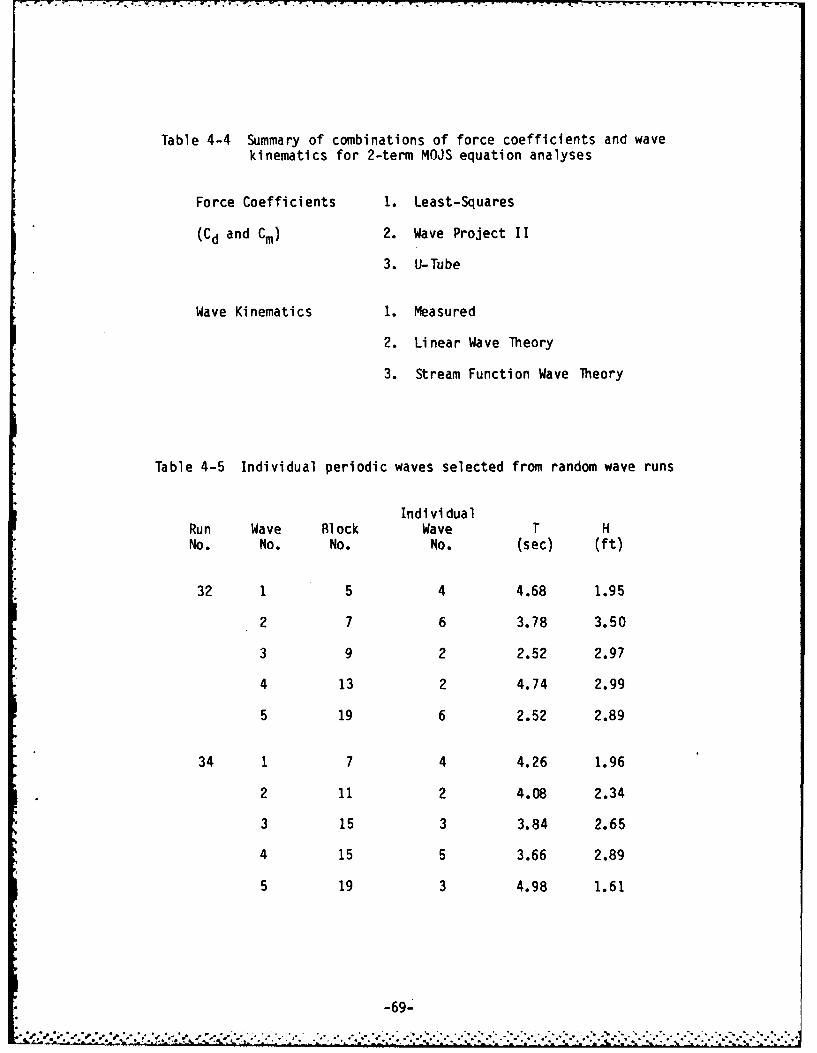
Table 4-4 Summary of combinations of force coefficients and wavekinematics for 2-term MOJS equation analyses

Force Coefficients 1. Least-Squares

(Cd and Cm) 2. Wave Project II

3. U-Tube

Wave Kinematics 1. Measured

2. Linear Wave Theory

3. Stream Function Wave Theory

Table 4-5 Individual periodic waves selected from random wave runs

Indivi dualRun Wave Block Wave T HNo. No. No. No. (sec) (ft)

32 1 5 4 4.68 1.95

2 7 6 3.78 3.50

3 9 2 2.52 2.97

4 13 2 4.74 2.99

5 19 6 2.52 2.89

34 1 7 4 4.26 1.96

2 11 2 4.08 2.34

3 15 3 3.84 2.65

4 15 5 3.66 2.89

5 19 3 4.98 1.61

-69-

" ,.. .", '"".", '-" ", " .- . * . % . ", ,. ,. ", . . " .*. ". ', . S", . .. . .' ,"." - . ",' ,". ,". - ' -

". .". .' -'.". . ' " .". ",

8 C; C3 Ns CN CD 0% C; C; 14 C0;N 0U N 0

fi C Ci N fi N 4 0 .4! f % C C! 0% cC c! C

N N N N N - - -N- - N

*0 C> N .D.D 0 C 0 C ; a N C; in f

C!C0n CD C> N0 NOW ND C fND

1! C n! 4

fi C N - - N - t C C - % C N- - % - C C -- N - ~ -

CD c

NO 0 Ct - CD- C ; c; COO di m d CD CM N6 C d 0 C N

O~~~~ w CoD o 0 0 0 0 0 0 0 0 00

o 6

az a0 0 0 0048070..4v 000v.

No 0

440

N C fi 0% NON N C f7 t- 0% C C C % C C - N C

- -~~~~~~~C -. . . . . . . . . . . . . . - - - - - -

i r n C CV .-. jN C ~ -e in 8 V$m %c1L 04 ql Ui. Cl c"q rt

0 i l IS IS 4I 1 11 1 1l 1 1 1 1 I I1 4 # I f C i C I

4mm0 Wr L k c m n- en Ln 0 c q VScC kcf 4ON L... in 40e m r inus r

c- ig 80 00 123 c o48'l 2 4 0C,000000CC Cl 0 Q C)cc do .

,j v u~ caue guji%1 uCJ.lJ

1..) 0000000Is! 19l i ~ O 1 C l . - 0 CY CY -W r-cl OSJ- CC; 0 ,

3 cm eggs 0 dm-mli, m SC;88C3 C c

301 0% Oen -rao 0% 0mcn I--p ini0 %C CD CD wl 0 CuoOa Ch0% DsO 00 fn1-O(Din - r, C

Or-r-.sw o n Ln W t -it ~ON m in %CMD %0 mi OCLn to in P O -* L I C0 a Cl CDinn nie aoo~ a 8 d du ac)md D CD400CDaC,0 ---

%'A - Z

C i L. ~S c- " C- - ~ .Ou a" a a ,i- n 8 C, %n nLn> . 00 0 0 0000009199: 1 9 C!.C 0 0000 0 000a 00 -l 00C0

CL :9 .9C .9: !... . -n ..J(-i . 99c! .. 9 9 ll C c. 00e. Cr=00.-.

,a in c- -" k- Ce-i-.-j .- -i~. -CJcrm e

*~C.

>wi -SIg C 0 MA W 0%

o IV

0,

'0. 0). 0 % (% cu v U v (i-4 .- 4 (% ti nnen i cu cu O iniinninn

*W vi I. GoJ.~.-.4- .-. OCs 0v Ny m N N N 4 % J ci 0,in ~ ooIt! 1~ 0,r r r

C - d.C,

£>* 000 00 00 0 0Z00 0 0 0 0 0 0cmc ,c 4C 0d

0dC ;d8d88 8dC :c :

ZUa a..'iC)~0i n)gi ~n swn n. ~.. O~nn 0 %(0..0

oii'ii i l l nl nL O l ciJCJ INN 9N llne. 1t.1lt

f, Un Nn OO- %CinWl n n n.nto0 i 000 l C 00 0o 00 0 0 0 ..

IR-*0 ~ 0,m

en-*Lat , C en* nt % V in k u- C mnniinnWi toN.J- kcsjcuV u0 %C I-

Ne0.

m m ~C C.J( -i w cm 'nJ .- CD wf rfl 0 m ' CJ w (%J -' - - - m~ 0 m. In Q~ m90

C- ll 1) U C0 C! I C 0 0i 1%. C9.. -~ (9! ('I -: !9 C!191 1. Q 990 cz:

I IS I I 0 0 1 1 1 1

M ~ ~ ~ ~ ~ ~ ~ -W -n -3 47 n I nM- (,-J C n n"mm -Wc W- - (i%

Q ~ ~ ~ ~ ~ ~ -C4-% rI n-- , t - a - - mo- C w-qy WIS qr L

P. m 9.. r C N IqrC P.- 'fl '0% II . Dc o- - -Ga .In - p m - -c .jCiI , %0I " ' C . C c C! 9 1 !

u ~ ~ ' C.- 0e8d8C ;88d8C 34 3 ;d aaC 0ada C DC

d-72-

%0 CD v- In 9, c ,4 CD i l .-o M . .n ." CD q 09 WI I )e

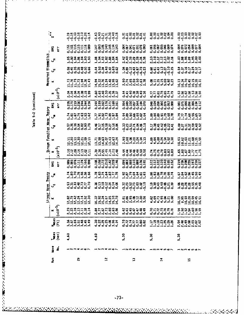
CD- -" - -W .r N M M -a-1a caM =I QC C D a4 MaC

C;s~ CDCDdCD a CD C; S S to D c; Cc, 4CS SD cS CSC 4C Ic DC

U) Ln Go4s-~ qt 4" IQ co NUqr CjC %0 oI~ o C MCiMCj C MG 00 i4j 0: -- 0!- -0 ---- 000!1 1 * l * 1 1 ! 1 ii - : 91 9 11010 :

2; Cj dcd oo 000 00 ooo oo 000 00 0000000 jC4e ciej Ci l Cqw;

4j, LO L.OOOO t o0% t0a tC %I V tC ,CC "r to0 -W r4 a ~a -W cy

Ln-t McnqrLnto Lne-W qrto o C jco .ac co C~aj to JC' -c cyJ oc"sjNC;8( ;C ;4 ;( :dC C 3d 4 ;88dC 38dCCI8

cninfl"nV0to .t" o ,t in cv d-. ,0 en w . nC M..r nin -

-0 - I!- I!- V! - -i !V

L4JN C; .0 d C0000000 40000008 o .6 C -..-;

P*- gh = toINN6 to-~.~- " 00 -W0 0N0 0 0 w 0%r - nt

In

* n M M.~)DO LnW0 , v- nC , 00 W It CD ". o4enMunId- L

0n UIF.F *-n- -n V o ow m r0Pw - m U,Ifl

I" N V . Ii ei CI I1 191!S1 iU

C, -v - w- - M -. 4 M "- v -" M -r %n -n -- %n& D4AfS.. .UU~~~" .0~fIO0) )So~-u

ce6 -4 cli r - h a ~n nr'* c .0 'w Z %ar4 Sc PX U) 2 (5. f-Ilc. .n c t00 00PC'%0 eU)U Ft--

r, Ln r -.nO.0 ~N NI O ~ ~ O0.O. vNO) 88Om 4 r04 . Me9K 1 l I _ iC i-Cc 4I 3C 0C ; ( DC ;C ; dC o 4d44C S 0C ;6C .C

00000 0 000000m W " Mf w wP 000000 M a 00 00 w at W 00000a00

q* *00IOIOIOL mw oa c st4 ' RU I 4nC~ to(D LI Po~l 1%ca~ 1% -:01 CL

. . . . . . . . . . .. . . . . . . . . . . . . . . . . . . . . . .

~~~~r a M M.- ") M~ C' .E)a r- P . -a ICM v.. 0 C %C - 0.0 M )~

-j cm - -j C4 " -c -- -- - --- -

8 I LnO " ~.'0 'I ue)Ul 0% 0_-NU)10,0%Dg. W C0 N0n,

40 0 0D o0 M c

IM Mi -WU)CM1 n% r T Wt 01 rU?4 C W# or

10.

-73-

as- - w C- r- wr m vJ (NW cm C-4 rO O r (N- 0%LO

0:r-% 'waad 0QCC 0;MDC1t m'F ~ V C DMC W l r 0% y

41 E 0%C5 ho t * 00ooU00 ocn0 %(A00 C o AO %(7 0cC%; 1: 4 4 1: ; u.4 .

mrcocn tLor-r- %0 r-w o W % rtnvNU' ''

0 ------- ------ ----- N- ------- ------ -

* ' u'U~ll JN(t r%~ lC)NG COl.l C .17 ON( O

Cu, C4-- i- - - - - - ---- - - - - - - - - v-Q'.L aCO nr nc U D0 na C y - q o8n tg k~ I

CC -W N~ -s Nn 88 s 98 8 8 S (NJ 2 2 N N - - - - - - - -

c'a ; 6d a D a;d' C aC NCD1Q 40 C0 CS C38dC d CSOC a d ; d80~(.~ N

C/r m "0 WC LO r ". . *- WN r w q N ~ CjL 9 ytCO o 0

6 a ~ CU CD c' d CC2,CD40cn adc' d . c ' . . ' aC a~-CCOO IJ CS.C0 a a

GD ----- -------- - - ---- -- - ----

%DwGD R mr 0n w'JN O.NN m m r C'" % . M~U O L k nmmf

-m-c -- m -4 vC ' ----- - -- - -- - - - - - - - -

8 C C CD a0a(D a CO CD d a c N 0.C; .CD. CD O(.C.6-Ca 0~C CD a

E~ 04 0e 0omc n" t t oam0 n 0 0nQ k z mC Q%0- C-) 0' 0t 0iO 1 1 : n1 l C

I-o '0 tot '0 (%i 0% -t nf W r 0 LnL * cn DwqO%

8 C3 8 o 0 a. 0SC Da4 ' 'C2 10C(Nw

m -rC,- % l nw o l0 01 1 MW "maCD mm-74-hA L l)L

m ~ ~ tOO U-)U in-U)O CP Ca G C i q c n % n C m-PMfl ~ m qw "La -aii- cy cl mO C.c-v . 41I f 41 Ui U

C ~ ~ 40 0 4 co, ) C3 6 d d dCD.*0'-S 41

'A- -- - - -- -- - - - - --c"en-00"it)to CDCA- at Ur 0% 0% Wr=WCS o (3h 0p- )(F r gU0~.i

aD& CO ) ~U) to m ~ r-1I %00*U)U-)D . c" U')4 (C -4-. %0 0.

-- 4- --- ---- --- -~- - -- - - -- ---

x " ol c ~i C4 " Cc cJCU c JC4 . C .C.J.NC.-' --

" ac - 0 L oL CO'r %nC~i C -?rO tn -41O m r r W.m e n L % w

U)j ". W.. LU..4JN 1 01-) M U o y %w D)p-V%P- ,.J %C 10 r 04 D% O W 1WC G 0r c or %m0

Go m 0 n0000000nC- r t 000 00 000000 t 00000

%n La . rVr0%1 ml - w - w- r-- - -t -c -- %- " -a- r- In r-- -W! 11 E1 l l ir .1 l tl !L t ! Ir 91 %1 9L

OtQM* C -L .0 %DI0 ).-1 m~Cl~t q.C0r- I0O "O ). -W40riO C e o coL- % *% W l Wb %0.w. C t r. m JCM, c %.C atCC C3.-4- 0U)41%0lr.U)L. - - !l C1 ! I-I- -:l :e4Iac

c1 000 00 000000c0 000000 80 00 00 0000000 C C C. 6c

J.:f-)C; ,OdC dU0i0- i0 Oi .- ~t; d8O 0 a 8d6d ;

- "1 P 1 ' C -: "I-- F, - - 'It -- t- 'I - c! - n - W!r

43 6 CDWC'U4 L1W 0 -40Uir w Cmar-v C t , t r P

.ifl CL '0C-iU)) U)CJ.l* w~ -g1 iO C4 w . . .

kc - %n".rr, q 000n0000w aK 0 :0 :C l l 9U iC l l l~1La .

14,

- U7K ~ C cl cms~J. UN SCJU JUUCCN ~ 4 -

cc) 4 ~ ~ ~ 0U) U1. N O C O

- ~ ~ ~))ff~ 4~~1~1*~4* ~q414-75-E )C

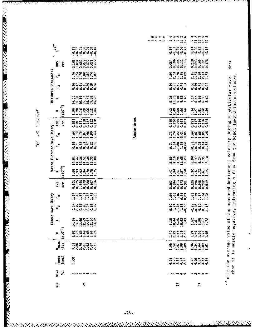
Cc 0 Lo00 00- c~r )e0% m 3 n c) 0

-4 C C, CD F-D CD- &Im C ~0 -W C~O'j04f

m. 0 0j CI 0 0cn c C % 0k

Cc 00 C! IC! lF-

L) . CD Jv JCsJN-j

%OF- 4OM%4 enC~ F,~~-0 fn CD0jF-~OlF-CsJ 0F-r..4003:

u ~ 00 0 0 0000 0000 n-l % C irCD( D(SC D, a C n=C

L.1

Z , -l ~ N C ~%n rc uLO8. 4 n - %

L- D 4 0 ) C% F- cm4 0 0 3 ) o

*~: -J

c.l4(%4 m tr 0 4CPV , -0%40Ln LO

%a m--- c (D.. CO c 00 -- - C

to tdooo yo q...no CDoomoa.to w

LI

-~0Il -O .40 - ,C

C; c ~ , a C2 e-. d'. 0- a-~n * 40 Q-

cu - - -- -- - - -- NC - --- -

- Cn m0 w a . m F-. q0 w~-~- 0% 4~O 0

> a,

%0 w cm , w r 'Cw 4-J

--- -- -- -- - 0 - --- -

%0 W- 40 W 4 a 0''D .U NNc

ri~~ ~ ~ ~ In ITII% 4M n enr

L .4 r4em e

@4 4-4~.C'0N ~U0N.~ .. ~F-76-4.

-~~- VnN mq7. Wr ;-Z IF.. j77I

,a-

A, 'a a .. ..

06"

..- .. t v .f .4 W!i0 ,l - :...-a a6 aO- =- 0 a.r =~ COO -C 0V%

.- - oc Wadd8 dd 0000d ddsS aaa

sr00-g.ZZ000wh

U~~~ ~ wj ml~~P~- N C4 -O0~ O ,NO.- c

I ~ .. ddaddd doooooc 46ae ddd .-...ao 44

N 0 .02. .~On

0'0CO

'a W a C m 40%9 , ' N,-- N.I VN.N !I

g. N 9o44-i 4 c 0"3,c oo- - - --q 4 uWr c m C4A. 4 no " '

Ve n 9.0 .D~ .0*0C- "n ;;!$.a 0N Cl cm "Vf

.. " a CNNNNNm o 0000000 U, W0 ~ I

~~E4I It 000 00 od%9oo 00 00 lic::Mdoo NN

C ~ 0 W OC 50 555 .eO500 0 O~rar-N WV"Wc NN N ~ ~ N

C0IWNN 00 0C0 N0-

01001.flwww M10 01i01 00(4nom0 MN~wonW"

x z - :v It to -0 Na: IM wtw sS!B~ss Vs~ r

0 C2 0 -; .-00 -Io.... . -o N 0 .- a- .

0 ":O d C d add2d addo~daT dddo j D--

E-4 - -

. ; oodd ddaddcd ddaddd dadadd 44-."

ddao d.**j ~d~d~d dddaodd add-dodz

-6 - - - 0t tnt 9C 0 1 aad ~ ~ ~ ~ ~ ~ 0 dC t fm~tJV~%W

In'

odacidod01 50. 10NN

~ a~oo oc oIn

-ffV~w ocoococlb .0.- .-. O .- w

5rE

-77-

w ~ ~ ~ ~ ~ c I' W3 00 0 0 .co-.Ne 0 0 0 00 0 0

to kc aC - DaC

a, a 0L 00 0000 0 0 . . ~) i, 0 000 0 00 000

C0C Sc4.

- ... wa..Nin-O 0NnO~n, a-~..u~o in..,. ~0. .C!

8 66C - - - - 6c

C~c~' in m <nNNai m ~ in iniivO JOoi c i Noi

W ;C D ---- - cm~e m 0. 000000 C; C d f Q6 ma0S

< "!000 00 0- --- iS n 00 0 0 -o --- D DCS - --

in~o- W W fl CD00~ C,00 n Q0. i 0 Q0 m0 - - -

c .0 rON- m 0 000 .-. Ooninin ----4 - C ~ s Q Dm0C

00 0 0 0 0 . . 0 0 0 0 0 0

Z d.OCD . on CD q, nC3ini m n.i m n..i YD.O n -r CD.i '0

10 1-i_ J % !I N 00 W!en 0 0 .. C: I'! 00.00..004. 1 % l

-t'- -!- - 9 - - !% ' 9C

Z M0 NNNt O Inn M.in M0 .. N~ W0 4 r4 M c0041m"C C 1 %ay -4( ;C Q8mQaoc

007.0 -N m10 00000 O 00000

IC 1% ll 0N0: ! 0 0N: Ne,. Oa 47:..- 000 N a. ! C001

4.- M:,C W, mn .-. iD -.a . . 0,0 W in mn N 0 a. in W. w. ;; W in m0 0 in0cn Gin a,V! 0:noiii V!Ninni 0 90It0.-!..-n.00l 1

-3 - - - -..-. jejn o o0c.ci1. C CD C; - - - - - - -

:t-.l~ o-ainn CD C N W 1rqe InnmC7 m r W Q a Nen a a0CDC o c C a C 6do od

4. 'W Qe~JN e aa~oo o 0000 C o ,0 C ~ wO 00 0 ..-.. 00.-

Wk4.m% WW4_n mr"Z 00"0 NNI0N ;; 10 " " o 000000 0000000 0W in-1 0W nW % a- AI l q 0 I % O A 1 A L

in 1 C., o o os OO Ou., 66N.-~ Co0 00 C;C ; 0 ;d ;c dC03000dC C ;C3 C ;C; (

a<UccCc -m~~cc 00 0 0 - - -- -nn 00 0 0 0000000

4. -,

-78

07. F. -7 1.* r_-.-!. - -, - - -.. . . . . . . . . . . . . . . . . . . .

do -W W -W w M__ s

C~~~o cC6 c C30 -,aa g .a.'.1 0 0.

'C ~ Q~s . Q 0 N~W4W .Wf~0. %n 0 0, W fl0.0 m am .rC-, ~ ~ ~ ~ ~ ~ ~ ~ : fn V4N~U09 U NW~ NW E~

- -.0UII.U' ~ 0 0000 000 800- - -N

0.N.0.0~~~W 0 C'. enf .NW 0'W..00. m --2W~~ 0j N C4N 0~..i.!cog.

-J.C4NWf" fw4w i ; ;4- .0. l a.N m 0 .0i 02 d..00I,.

O: otm' CD w v04 C4 r;- -44 0m W -0 mI F0 C40. .w00"A m r~a

us . w' vw.O~0.0 M.0w3..00 QO..Wp0 9Amm m

"t It - % *~ .0W 00 0 ..

K~~1 -! .0%0UI0. G!.. 11:0 .0

al! 0: s0 11:0E ..... W! It 0:~~UI ~ ~ iod0. -: doaS on," m,..'. "I em.~ A om. .wm

Alo "0 p ~"!1!.-V lI ~ ~ ~ ~ c t w...q.. m o o d dco.. .i~.,,.w,.

- - - - - - - - - - -- - - - - - - - - - NCD C;' U~ .0 CD4 ;C ;c9$ CA to @..o dd do o

41 .0

9 V!g...~ It . 0. It C. PI9 . 0l 10 Im . .0 .-.rs4 n 4o Mq A (4 .00 . 0 0 d~M~~ c; 416 in... --

a, " mq.Jn co ' ,..ye 0, a.'" co mmeqo , e0..I.. U.0es' ",.,~ mq - . 4 a a.m0V

-0coc % aL 01. 0: 0; 0 0; .. i p-;a -W NaamIn W)a~ Nws

-~ ~ ~ ~ ."I So lob -0 C s "Do 30 .00, 88m8 V ejostZ16

emmem ...... em:- 4% A4;;:;ddcS6d4c6d00.4' fm~'a. -

-e - d~cf'cNNoc4 d 0' . @o a 000000.....

UIC PNieI 040S. 10W0~ %1NP.0 * -e4* q5 Ar JN4 WN 0-Q N J.N dc; 4i D a f

- ~ ~ ~ ~ e In d d d~d O d O d O

p-*-* W 0.f.00 mPI~nn0W.-79-d ~ P-fPJ'

- -4 -O14f\**f -nO 0 O -l r.~l - -- -Ca.-.0..,Cfl)CD D - ------

N. 8g -=fC, W- 0 8 j % mC

.0 -Z. - -jm

K;~~~ C4Um-.4- c; 4 N.N:0o 4

V Nc g a- wc m a 0m- m-0a w

c10 m4 m-~41O~ - m m NalCUo~N - a - o-.

CQ a:r 01 D N10 a,~0Ol0 v.~* n -0 a NmOm-m

~ 1011044 00l0 01O

-- C91 co-o4.o -lor tnQ r4Nr.t CW q ,0>4 ~ ~ ~ ~ c c4 N004tf ".NL~fle -. 0 ""Mm4 ,-fl0%%44 -00

wxa , 1 r 0: 1 1! 0: ,0.OrNr I0 N. O r NN. aN NN: f C flt 1 4 4 4100.1

mm0 ' e,-oo~n 0n n..~ ---- e~--- -------. ~ - -.

a -o O1IO 0IL % 04N0 w r.4444tfl@Tmhm. Oo0.a-00

1

a,. e4 m-.wd

411 -!- - v

4114 o4 m M'4 Go~.~4 IO4 0 0 r C3 0 0, 0 N 0,z mN0 m m C. aGo

.0.-lN.NU .a~rt.-M C .q0,4.- - 4 A---- ---- 1

m ; :: m"0 1 a4000.404 000 0 00 0 4 4 441%N C1S 43 It 0 !." 1 l 1: 1 ' l C I!1 l

(M K a1 C~,1tli04 .090.4.4-.. 0 . !~ n C!104C-r.- 1 44.C!-oo coc o- -m40,c cc 4-4 ',m- n - C

- - -- -C.- - n - Q

- ..( ~ c co .fr-000U,. m 4 wo ---. e a,... N m4.1.4 m 00 mm w n.

a a~ =-N1E4 N m CD CD -D-- - - - - - - -N - - --3000

vl 0%, '4 m,1

10N 0011 . > w n A m U M,,.Pa m flcaa-

44 W', -- - - - - - - - 0 0 0 0 .- 0 0 0 0 . 0 0 0 0 .

44 . -N41 w t"1 4.CJ0..4 '~444 1 OI14N..aa'- 10 0'n1.

-m44r,.o ~.e . cl O..104-.Nfl 0004.OCD

4W Q M.9 .Oc .CD 'a -W(94a cm a~a@ 0cm m - - A

II ~ ~ D: CD - co f9fW~~J ~ n c,0.a cc99U QJo m

w - .nM MC;.w c j C4c 4 c hwf

-o - - - - -

U qLm W- 4r 8 l%4(9 -W w -.- 0* m- U -~r...-.0.f0.~f a J.40a ft..~9f W, -W~~a

mKmm --- --

49~ ~ ~ ~ ~ ~~l C .4a. .ie.~.ft "w M W"*f- ----- .J9~ - CD*4 0 0

a G o- w: w . a .d oJ -W W W 4 0- - - 0 . - , u o . - O02U

I ~ ~ ~ ~ ~ ~ I .0.0-9U'lf0 0...r 9sflo

M-cmi m- 0-aC.w0 m -Or w 9" a. 0 m~q . w.. w .~ Ir ---

.9 ~ ~ ~ C4 Wb In~9O9- m .a ,- a.cm aI 9-

3 ~ ~~~~~ - -P00. -~.~~0a - -~~q -.e~v

-j 14 m 4-w .. QI X-.ijmam m~..a hnm

.5- .DV.n em e. rW WG %v ye 1

WC-o aZ n 'f~la .0 010,0.-2911149 .0~ 0

9',h Z -' I

wn 4m4 49 .9' C DIfi. w O 0- m 0 i Cc. c"'. 0. U,~ .4. 0CdA a CD

r4 4 .. sg m a 00- --- - e cm. .. fto 4~ d - m" -

i%., 2a.ZZAS. -. m ... 'r.a g!e~ M0 S w: wcc 0 'a 0 9.J0~. . 9- MD a* r

C;.-..- 6; ~ .0aa cl==!!=oa eo6-0ci44 444..:.-- - - -- - - -

V, 0fl~4 So a ... 0v..-989'9=4U 0 ~ ~ I It .9 J .. ! .0 9 91 . .0d~. a.l . a-

E, a a W 9-..9Pdn f Vb -A 1-.0 w - 0r W r bW W a .0 w rwo -. -r w -a aD b .%9.1w0fl'A.%

IC A a W a.0 01 I I WtItC j 0 -s-... 4 o. - .V-t .a..oa. -

K-

K Pmm- v -A..0.. .0 .0~ mmm..-wA a -0 - oownw 4aa

a~-C onj 'a ouc-r .a i a~. d - C 6 '

0 00 00 roo, w: : 0

U U90:00 9-a .... .. . . * 1 1 9

W4,0444. 44441"Mme~ -*909-.ww -PJ990Uw 0-w -10.fl50

*~1 t,-.4P

-8 - fW Q "M %, ft rno

1C 1! O ~lOlfl% M 00:.- C')fl'JCLnr-Nwo~om gro, 0 n .nno

a - N N*4%O

o -"""wmmn M q c OD a

.C -D 0I'n.c tf CD tOtm t~

Co D -- - M-- - -

41, -W 0OCN . 11: -w

mC 'A 4000 c 0%tD tM

to. 19 C%. !- c1

doN cJ NIW IC~. I.b~f

U)0 'A Wr.N. 0).C6J a fl0.-m a,

00.-.

1 W0 WR It I

AC! 'A InCn~.O In~O '~A0C fl W!%~t U weot 1% oa! . '! O

CD -- e4C t W 0Ini~.

c co) 'A aW I OC'J1%WC, 0..Ii .t

4.,

3C aE w F.

Orin m 10 -4Ym m 0

zjw U) It~ t

n*:1C - M 10-.t~~

.4 '4 w N10In00. cao Lnsom .. ct fl'

0 'A

(A ' .CO00 cr AOnL ' W ~C~~a NNNNN 1% In'O ..

41p

> C4 m .- N- NN* 0

m ) ' ~ ~ 0 0 r tOn-n .. nt~-

cmOO OInO0 0r- CJ~

~; Ti ~ 0O~n~to-32-C

_76

,- I

.- =- eee-------- caiadJ ------ p p"pWepjpWp jlfaifa

I~ . .*dd~ .e d u. .. .. . .e.a. . .-...

I jci de@C j *flC..C

-~~ ..... C . . . . . .. ..

T l - 1! .0 1!1.6 . . 11

. dadddd doldidd d6c' d deald .ddddd .....

mz --~ - : 33' - Z~ u!"!, de .,:d d~e~ ~ dddad"

lo w w C2 ~ ~ . .

* I V

4" 4h..~. u . e~ ~ ~ . e~

0N v W Ifm wo N v W W v e

* UW

*-83-

F~. 0..o-orr I 0; .- 0W.wmm W1 -,D - -

w I IFWW- m

07 6 6 0 867d Cdwdr,410 r)00...CC; .. 0o0- OCON.7 a

L L O..OL.-LIO OOC IC 'C CCC CC 000 =004. oo00 o

-1 -N- -- - -- -- - -- - -- --- --

L0 000006d 00000 odCdde0 dd..hd 7 do$ddS

. . . ..4 %I . . . . .. . . -

41~ -1

6 C; 6-0 0 0 d 0 JN3 6 r.INN4 0000000o 00 000

So ~ ~ ~ 1 ao CD.lrrN -t N1.- -C -Nf71 -N.- l N

S I!

5.~~~1 Z;; .Ott .. C Al..S Z1 Z7. CN.r Z'4..08 C O

00000 0 000 000 0 0000 0"000000 0000000lIl :li l, *.c!' ' o :1 1l00t..T1.-.444444 g-.N,..OONI' ---D~ o -1 -i(0 C -1C C -

410C 141l N N-841-. ( .0f7. 1 7't O 4,S C

44 - .CS .... CC C. . . ... C C ....... ...C

----- -------

u

. . . . . . . . . . . . . . . . . . . . . . . . . . . . .. . . . .

'.-LI Cr'r CC 0 ... .. -. 0 0- .. r, O O 4 .C

zm n - I

* .4N .4 'N .. C C O C 0 . . . . . N. . . . . . .C 0 N. . . . . . . . . . .lf

e f rngfg.. " n' N .. . n ...... .C ..

- -- ---- - -

Ioo ooo 0 -- --.°°-fl C .. 0 C C.. . . . . . . . ..0. . . ..0...NN O N C 4 ~ 4 %...

• = - v. N Q. S ... I .... .. 4....

00 * 14 Z; 6,6 Cr..C;d c a 6td Z9 Z '1O.OO dcN4C004?

0: . 0C0 .. 04 °4 C!1 !-..IC!

35 4 0 LI v-C f4a .. .4 4 4l N lN

d o1 NON C; ; C 0 ~.0 0 .. 4C 0 40 a %0 4C3 0 0 .Cfl0 C; C;.

---4---- C.0.C --- -- -------.M..M1 444

- -

-35-

",'.""..'2 .'2" ,'..''. ; ".''.: " ;'.0.'" : o. 0. 4C4 ,00", -, 0 .. .... . .,,,-, ..... - , • , -oN . - -, • , ,, - .0. _ ., ,

In ~ ~ ~ ~ ~ 1 :C n- n-.'...tnf nr .a-tmJ..% 0.ir.n.U OtOo0N *N0 I

c ~~~~ wo 'f5o-gc4 w 'o m fCt w w 00 0C

0 d 66000 0dr60p6C5 o006 06 , tt0 a 0o nn000

-- - - -- - - - - - - - - - -

-- - - -- - - - - -- - - - - - - -

E,,4,0f 0 0 0 o,0 000C0D0 O 0.- ,. % (02X0CM

M0 0 000 0 00 0

:3 irbcoo .oo,. owo.cm,,, vtc,eo .oo ,no oc mn , O ,tnooo'

a -r------.) ----0r ,-- -nf----r-- --- J --- f---~r-

0"nnn tSfl Crtfl8l C800 0 ao d o 4, -0 ns'sn,n

-~~~~~~ -6 t n - -rf- -~~0.J-.r -f~lnC',.. -- tcU"e -nCJ-- -- - --- - -

a C; C4 C; C3d_4c;0C__ aC; C a0C>0 __

I: C 1 "I.C 101:l ! . .. .2 l n l l

og.

,°o000000 0000000o o, ood o ,ogd o o dooco~ocI --05 0 , O 000-0I 0°°00404 bo0eatn0° g) 00 -0 .0t00c

I-86

' oo ooo o~ oo o~ ooo oo ooo ooP1o

40 0-00000 00tfC..ICt0 04-00445J Nd f,..fflf NO%01004

°0° ° ,o ° 000000 000040 0000•04 ~

Li t

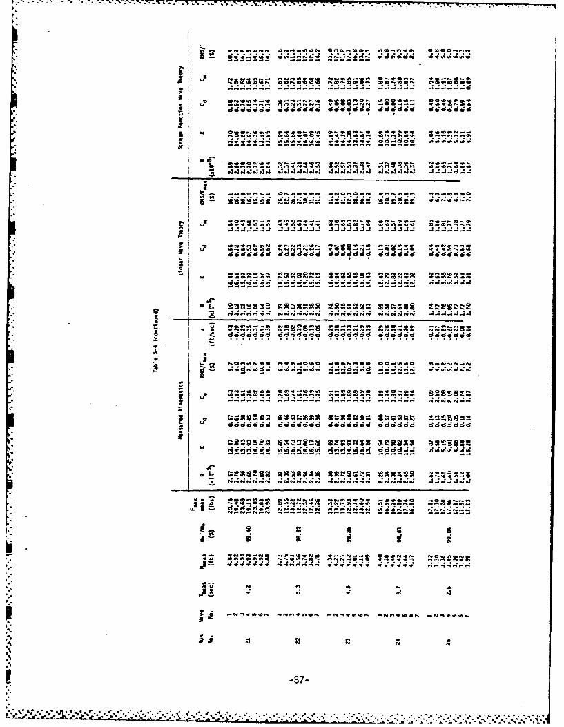
- - - ------ :j l

.- .-.p . t 1 .ri. '1'!- -o

It O

.oWM" f sqZaMa..p agz., me g s : "M

I * I...l.. l. c. se .nn--.. ..

I Itdocddad ddO.iC4.C. decenne ad'idod S 4eedndne

Vn .1 .4444aa d~jd -s Aa-fe'-

a ~ ~~ WlllPPpaaaaa~pdO*l1e~c 4444t

- - - - - - - - - -

I .~CtS% C .l~4.S .. an-~l *.t.l n e e

-' ~~~ ~ I It Iae. n.s-- epee 5 .. as ..

J I

-87

6r4

a. m eg !cV. c m

.-. 5O0~aCD WNO 0 1 W1006'

68.It

d. 06605 C2, u.,a:

41 - -.no~.. - ~~m- - W

m-. ONI,o5 00. . N 6C

0,4,1 wmo.-..

6. ~ ~ ~ a: A, I*IN N O'nM4

lowm d -"=w.

6T z V6 66 "

WW M IftlN N * N~ U..

wa~n~s. 'o4,

"6C co m c a ;.:na. 4ao.

0.-.0.o~~c.- *N1.6 &V -0m c.

46~n V p -. 0N-

-.. d~cd~ I a-88-cd

8. 6'66 6 6

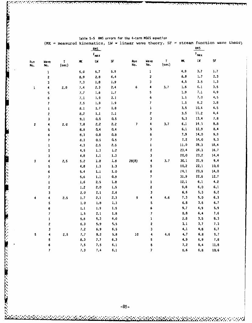
Table 5-5 RMS errors for the 4-term NOJS equation

(MK measured kinematics, LW linear wave theory, SF stream function wave theor

RMS RS

Fmax Fmx

Run Wave T MK LW SF Run Wave T MK LW SF

No. No. (sec) No. No. (sec)

1 5.0 5.7 5.9 1 4.9 3.7 1.7

2 8.9 2.8 6.4 2 6.8 1.7 2.3

3 7.3 1.8 1.9 3 4.5 3.5 1.3

1 4 2.0 7.4 2.3 2.4 6 4 3.7 1.6 6.1 3.5

5 7.7 1.6 1.7 5 1.9 7.1 4.9

6 7.1 1.9 2.1 6 1.1 7.0 4.5

7 7.5 1.9 1.9 7 1.5 6.2 3.8

1 8.1 1.7 1.8 1 3.5 10.4 4.5

2 8.2 1.1 1.1 2 3.5 11.2 4.4

3 9.1 0.5 0.5 3 5.3 13.4 7.8

2 4 2.0 7.8 2.2 2.2 7 4 3.7 6.1 14.3 8.8

5 8.9 0.4 0.4 5 6.1 12.9 8.4

6 8.3 0.8 0.8 6 7.9 14.0 9.9

7 8.3 0.5 0.5 7 7.2 14.0 9.3

1 4.3 2.5 2.5 1 11.0 28.3 18.4

2 4.5 1.3 1.2 2 23.4 26.3 16.7

3 4.8 1.1 1.3 3 20.0 23.2 14.4

3 4 2.5 5.2 1.8 1.6 28(8) 4 3.7 30.1 21.9 9.4

5 4.8 1.3 1.3 5 10.2 22.1 10.0

•. 6 5.4 1.1 1.0 6 24.1 23.9 14.0

7 5.6 1.1 0.9 7 31.9 22.6 12.7

1 1.6 2.5 1.8 1 12.1 6.1 4.2

2 1.2 2.0 1.5 2 9.8 6.0 6.1

3 2.0 2.1 2.6 3 6.6 5.3 6.2

4 4 2.5 1.7 2.1 2.3 9 4 4.6 7.3 5.0 6.3

5 1.0 1.8 1.3 5 6.8 3.6 6.7

6 1.1 1.9 1.5 6 9.7 4.9 5.9

7 1.5 2.1 1.8 7 8.8 6.4 7.6

1 5.6 5.3 4.0 1 2.8 3.5 8.3

2 6.3 5.9 5.5 2 3.1 3.7 7.3

3 7.2 6.9 6.5 3 4.1 4.8 6.7

5 4 2.5 7.7 8.2 5.8 10 4 4.6 4.7 6.8 9.7

5 8.3 7.7 6.3 5 4.9 6.9 7.8

6 7.5 7.5 6.1 6 7.2 8.4 11.8

7 7.3 7.4 6.1 7 6.6 6.8 10.6

9 .

L-89

- -..... ...- [.%* .. %~~.' ~ '.

Table 5-5 (continued)

RMS

Fma x Fmax

Run Wave T MK LW SF Run Wave T MY, LW SFNo. No. (sec) No. No. (sec)

1 15.1 37.1 40.1 1 26.8 26.0 20.4

2 10.0 31.0 35.1 2 5.8 29.1 26.2

3 41.6 24.7 35.5 3 6.0 31.7 29.1

29(11) 4 4.6 11.5 30.3 38.3 16 4 5.3 8.3 33.3 28.7

5 57.7 34.8 42.1 5 33.7 31.7 25.4

6 49.8 37.5 37.9 6 33.8 31.3 23.4

7 53.5 37.9 43.4 7 30.0 32.1 28.3

1 14.7 23.4 41.9 1 29.7 26.0 15.9

2 55.5 20.4 35.4 2 26.1 30.7 22.5

3 49.5 21.3 28.3 3 35.0 30.6 26.8

* 12 4 4.6 38.3 21.0 17.6 17 4 5.3 22.0 32.9 22.6

5 52.6 27.9 44.7 5 38.3 33.3 21.3

6 58.0 24.0 31.4 6 25.9 29.8 18.7

7 50.3 14.8 17.9 7 25.9 33.4 31.3

1 6.4 9.9 5.4 1 28.9 19.0 14.9

2 6.7 8.4 5.1 2 5.8 21.1 8.5

3 4.1 6.9 3.0 3 5.4 16.3 8.5

13 4 5.3 7.1 11.0 5.7 30(18) 4 6.0 21.0 14.1 6.7

5 5.1 8.9 4.4 5 6.5 13.4 6.5

6 7.6 13.6 10.5 6 9.3 17.7 8.1

7 9.3 10.1 7.9 7 9.7 21.7 9.5

1 6.1 12.2 5.0 1 50.5 25.0 31.4

2 5.6 11.3 3.8 2 38.2 27.1 32.9

3 6.2 12.4 6.4 3 48.6 29.1 9.5

14 4 5.3 5.5 12.2 6.5 31(19) 4 6.0 43.7 26.7 8.9

5 4.6 14.0 7.6 5 41.0 27.3 6.9

6 6.9 10.7 5.8 6 6.5 30.9 8.0

7 7.4 15.4 9.3 7 8.8 20.6 8.2

1 9.4 22.6 14.4 1 18.2 27.1 22.7

2 7.6 22.0 15.4 2 23.9 34.6 37.1

3 7.2 23.5 21.3 3 25.6 31.1 33.4

4 5.3 5.4 24.7 20.5 20 4 6.0 19.4 31.9 27.5

5 17.0 22.6 21.7 5 19.8 36.9 37.5

6 7.6 26.2 21.2 6 28.5 36.1 38.6

7 8.4 25.9 23.7 7 22.6 35.3 11.4

-g0-

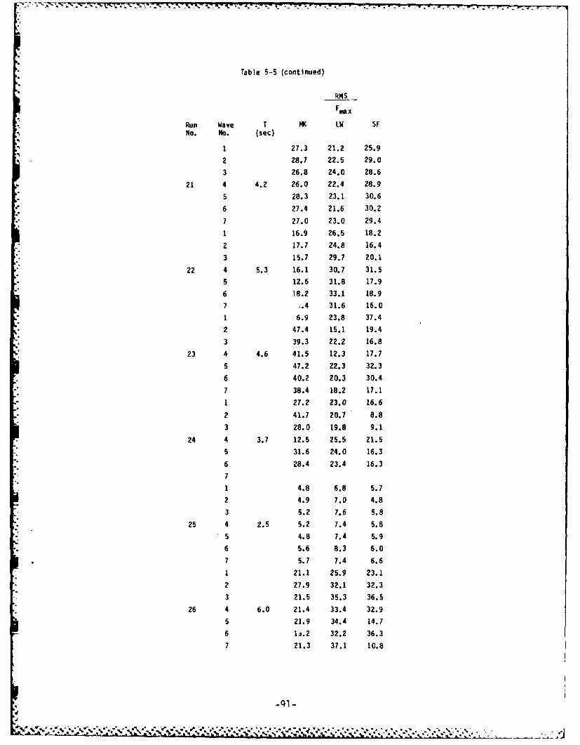
Table 5-5 (continued)

RMSFmax

Run Wave T K LW SFNo. No. (sec)

1 27.3 21.2 25.9

2 28.7 22.5 29.0

3 26.8 24.0 28.6

21 4 4.2 26.0 22.4 28.9

5 28.3 23.1 30.66 27.4 21.6 30.2

7 27.0 23.0 29.4

1 16.9 26.5 18.2

2 17.7 24.8 16.4

3 15.7 29.7 20.1

22 4 5.3 16.1 30.7 31.5

5 12.6 31.8 17.9

6 18.2 33.1 18.97 .4 31.6 16.0

1 6.9 23.8 37.4

2 47.4 15.1 19.43 39.3 22.2 16.8

23 4 4.6 41.5 12.3 17.7

S 47.2 22.3 32.3

6 40.2 20.3 30.4

7 38.4 18.2 17.1

1 27.2 23.0 16.6

2 41.7 20.7 8.8

3 28.0 19.8 9.1

24 4 3.7 12.5 25.5 21.5

5 31.6 24.0 16.3

6 28.4 23.4 16.3

7

1 4.8 6.8 5.7

2 4.9 7.0 4.8

3 5.2 7.6 5.8

25 4 2.5 5.2 7.4 5.85 4.8 7.4 5.9

6 5.6 8.3 6.07 5.7 7.4 6.6

1 21.1 25.9 23.1

2 27.9 32.1 32.3

3 21.5 35.3 36.5

26 4 6.0 21.4 33.4 32.9

5 21.9 34.4 14.7

6 13.2 32.2 36.3

7 21.3 37.1 10.8

dra

100 FIGURES

-93-

7 - 7

> 0

E~ w

CC

o to

4-1-

Iw.-i

-co I -

-94

075 e a/,. _ sting) dri to math Strain

top an botom 11

94,' I"& t1 an oto

T ' L 'l:I3.5.

Stinless rodI with low friction

4- o A./e~s ;. / U I , + ,barigs 2 PlacesIo ,..i Wes (existing)

b ingeastin

hol for

Direction of m *d

pressure transducer s,portal game. see details 1

+.r. E l,

4 smooth aluminm cover 1Skins. 12'- pipe. 3/8' 1wall thilckness. Splitlo[aludilly. Fill I Ikerf bit to 2"- flanges. W1

if

2* flanges Y(typical)

i" I I

S_,II OI

4 strain bar smll auto U-jointalunum towper 7075 TG with teflon IV"e

bol boto ol e for ItIfd I almnu lag

ELEVATIOIN

Fig. 3-2 Sectional elevation of test cylinder

-95-

"J~A leoL

Fig. 3-3 Cylinder core during installation.

Fig. 3-4 Cylinder core invertical position with 1/2of lower skin in place.

96

Fig. 3-5 Bottom (and top)support strain gaging.

Fig. 3-6 Bottom supportbolting to WRL floor.

Fig. 3-7 Skin installationat bottom support.

97

b."7

AD-RI57 722 HIGH REYNOLDS NUMBER WAVE FORCE INVESTIGATION IN A WAVE 2/FLUME(U) OREGON STATE UNIV CORVALLIS DEPT OF CIVILENGINEERING R T HUDSPETH ET AL. MAR 85 NCEL-CR-85.864

UNCLASSIFIED N62474-82-C-08295 FIG 26/4 N

* -. 0

111010

NATIONAL BUREAU OF STANDARDS

'S WCN*OCpy NESCLUflON TEST CWAT

e 45p

4. x n

strain bars

4 -5/8" bolts, rl apartial hol in 1j' plate

Portal gage rinqbase, 1-1/2".,not shown in sectionalelevation 0 0 01" steel rods

PLAN SECTION B-Bwater proof seal at &Waterproof connectors for pressure

pipestransducer leads

1 1/2" std. pipe

12"

A 5

water proof seal 3/4"-on rim and at

I" *steel rods threaded300 both ends

direction

6. of waves

.3" clear all around

transduceradpr

Fig. 3-8 LOCAL FORCE TRANSDUCER AND PRESSURE TRANSDUCERS (aluminum)

! I I 2

These two surfaces are 1 I II 2

contiguous when assembled

_- . 1/8" shoulder eachend of 1" 4 bars

,I , 'i , :, 1 1/2"

strain bars7

0 75 r& l

BT

(L 8 - 5/8" bolts

4 top., 4 bottomsee Sec. B-8

This shoulder contacts2" flange of lower5" tube

r.r

" - Fig. 3-9 PORTAL GAGE FOR LOCAL FORCETRANSDUCER (exploded view)

OSU Have Research Facility

*. .... ///141 ,.99-- - - - - - - -

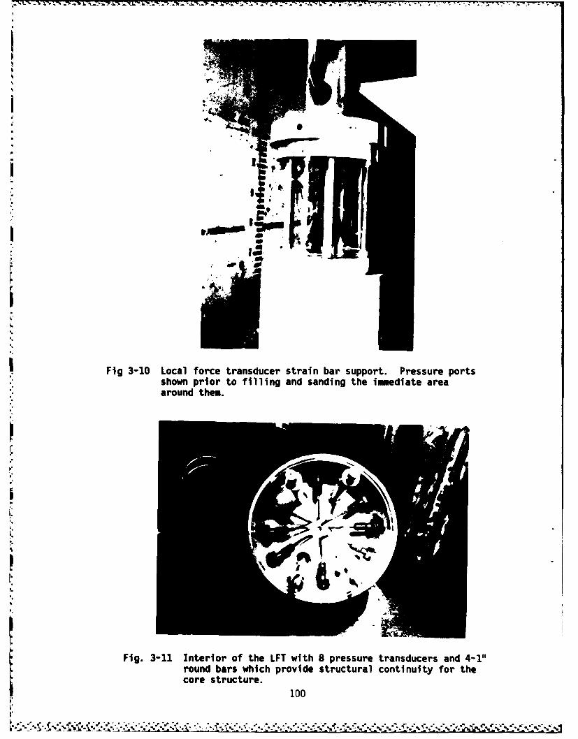
-, . . .- nn * . '. - : . -. . . ..- • . - -

I'I

Fig 3-10 Local force transducer strain bar support. Pressure portsshown prior to filling and sanding the imediate areaaround the.

.t.

Fig. 3-11 Interior of the LFT with 8 pressure transducers and 4-1",round bars which provide structural continuity for thecore structure.

100

* ,- p.'...* . . . . . . . . .I- P ,p aLm . . ~ ~ I* !- -%- ~C b..

Fig. 3-12 Perfect alignment demonstrated at one azimuth positionof the LFT, bottom joint.

... 4

F"

I"

F"

Fig. 3-13 The worst alignment for the LFT at the top joint. Offset= 1.1m, although it looks larger because of the sunrefl1ecti on.

101

[V V .. % - V -. >\. '

7 ~ ~ -7 f'Srvn VsE'6

dpoz

NCf y.^IF-SXti -8- AlflOi

III

At. g*Aa

A- i.r 0 -

LEAST? Sf3,.'lf : -r~

SYE gt~v'Vs" ~~r~ ~e aa I IA Se~

r /

UVIWM ILTLI S thO STIVVITV4 ro F'9

ffour 7 hoT"XCAsr z. IEAs .9

Fig. 3-14 Bottom and top support strain gage wiring.

102

- _______.,A-?o..7 '777 B2

t)F,

-- ,-

F-.C4,ZDr /r

(Lot^&) Nol it rd 2y

PAST Z I y

e Fig. 3-15 Local force transducer strain gage wiring.|..

."

I103

* * . * .* ***. *** . . **i.~.

* . . *r* ~ * * . * * .~U .. * .a

IN1 R1 I R~ If

Y1LYv2 E IN 2 R 2 AV + +V2

0171

Fig. 3-16 Typical suming operational amplifier

4. . -104-

.. ..........

, Fig. 3-17 Nearly completedinstallation with one of thefour skins attached.

I.

Fig. 3-18 Three of the fourskins bolted on. Final paintingand smoothening around thepressure parts in progress.

105..---, % :. ,,y -, ,.w ," ,,-' ..,oI. ; '- -'.'-'-'.,...."- ';'i- ') T-.-;-';-.-.-'','2'. ;-',;-';-,-2' '.-% 2-

west current meter

P(

east currentmeter

~hh.

Fig. 3-19 Final arrangement just prior to testing.

Water level is at the test level.

106

-I/ .JIL- T'f77c.,+ CyA.,uYDUL - 77,"_ W,Vw6- _

it

< t

ILL

Fig. 3-20 Signal routing

-107-

wc 7

(DD

SI

AA

Fig 3t21 Exapl of -XX Calibration

N.59

S" I

" -. cULo -- i

F - Ilcl

I -'I

.-

. Fig. 3-21 Example of XXX Calibration

q -08

Fig. 3-22 XXX Calibration to the east in air.

Fig. 3-23 Calibrating at position 5with the bottom support submerged.Also shown is the horizontal trussused for calibrating at position 3.The completely assembled vertical

g| cylinder is on the left.

109

........ ................ .......- ..

-~~~~~T 77-777777'.- - 7Z .1.

Fiq. 1-24~ Method of applying torsional calibration loads

-10

"2 4 p.*.*u*su5Vh'~*I . -. * S~. ' .- *

a.".

44

- -.

-- .~-.. .

-- -

if.

.1~

4, 4.,

N

U * 'a-4' -~

r ~a.*-.*J*~ ii I'p

K S

I

p L

* a)U

-j

"I

U,C

1..4-' 0)

GJ'L

U,UC0)0

~

'a

-, t.

e-L.I.

:~, v I

t .U-'-

I'

>4 U

I' 'I

+

U-

'-+4'

S

0

U I

f

____________________

.4.

1 4-

-112-

* * * * - U

* - -- * -* -. - - . -. - * - .

'.1 c r_

41tcu 0-S-(

(A >

.00

mw.. ..6 ma -uma -

- -

Fig. 3-28

Fig. 3-29

Fig. 3-30

114

i +r

t 1:' 1 77-

Ij I7l.

7. 17! ,T

11 .11T MEL.-SALEM, N H, U S.A. Wave Prof i ler

i l n rTF 7_

-4it7

Tk[ 7 1 !L 4 7:! in

4 +t

tj 41 Xt it

19-L

SALEM. N H U S.A. Bottom Force North

7a

7 'T I i:-,

T

tit AIll lTi!T .i! 11; !il I TI r 1.T,44C) T4

T" ............T

Bottom Force East1 ill' 1 .

7i. to4. TU.

;71 Zrj a

w! 1t, I r

a

SALEM. N.H. U.S.A. Local F orth

+T7 Ifli! 1i;!W IT ! :it; I

T it. LI

LiTmtt 7 4 4Ll MEESALEM. N.H. U.S.A. Local Force East

q

i0 ci; -q!

It 9

qu-)............. so I WH I I A.A Inns

Fig. 4-1 Sample strip chart recording for Run #5

-115-

Hoiona Current meter IRockland: Recorded

Wave Current filter fite Measurementu(t) T .159 sec fo = 8HZ m(t)

Fig. 4-2 Current measurement and recording diagram

-16

Fig. 4-3 Flow Chart of NCEL Data Processing

WAVE RESEARCH FACILITY

generate 9 track magnetic tape

ICDC CYB.ER 731

PROGRAM WAVE8

1. Converts integer values (0-4095) into physical units

2. Removes "bad points" from data

3. FFT data with fundamental period = 8T

4. FFT filtp' data with 1.5 Hz low-pass digital filter

5. Computes horizontal water particle accelerationspectrum using only' two harmonics

PROGRAMS FDATA5/FD5A

1. Selects 7 discrete waves from 8 recorded wave sequence

(FD5A = automatic selection)

(FDATA5 = manual selection using TEK cross-hair cursors)

2. Reduces data from 256 values/wave to 33 values/wave

-3. Produces a file of 7 individual waves per run

PROGRAM LABT4

1. Computes average velocity from measured horizontal

water particle kinematics

2. Computes C & C by linear regressionusing 2-term MOJSand 1) meaguredm 2) linear wave theory + average velocity;and 3) stream function theory + average velocity.

3. Computes errors between measured and predicted in-linelocal forces using 2- & 4-term MOJS with 3.-sets of forcecoefficients and 3 sets of wave kinematics

~-117-

S* . . . . . . .

Ix0a:I-CL

W w W

0 0. as

L' CO U! C L9.

CL. V CL .. ' CO IL CD '..' NO 0MinW in- V-0r").-.

N -W V-C CLL

a h CD -a-ILa -ci) -Co CO - U) CD -C) -- fU

-_W4 CW. IL I -COWI NoJ 4 w .-. wC - WCs- 4J

wa wup 4 5.,Y

0

-4 CO - *w a

9- M - W cwv W %Di %W

Ua OD W- a -'n M %M 0 * S- = a0: W I ~ C O C O~

WOi. LL I CD -S= C-4 b(! CDO4 NC- l C

N -a: - ,O C4CO 110 ID 00 I

IxJ in(O -Q -4- 0 =1f CO -) V4-) CO LL

CO~~~u. CO~R-CO -CDW -CW' -WCDW- CW'-C-1- 9C 9--- -aJu) - lT 40)@ -:Ui

9-) f.%Li-Ix WiW W- O 0* 4. _j 'V q

N' c in L) U ta OD -W *O CODI CD(D *-W in a: -- ( .,.4 - O i U

ft-W I - ...( J )( -= v U '" ql i"s~ r- %D Le ,L --- W -- 42M , M 0 CO

IX ( L. U M.d & ( w -_ o _ CO na -i _jj(j 0-1r

'- N

IA-c)clCie

.o

0641

X40 0

06'0

-. 7 _7 -

IL

P-

C2 C3

00

.24-

04-)

S_0

LL.C

-120-

Lo

in Lf

N Wcno L" LL

'-r~rI " ox

n L

CD 9e-)4l InC

In UD

tpw 0

CD~ZD

in,-C2Cl

C3C

q!.4~ b

I-122-

ILc.) 1

Mc0

*~~ 4- ~

4 LU *-C3V - ' >

4

.61

i. b-)0.00

C3CCM

-123-

LA.a

0."

U .C3

U .q9N

0

06It

-. q.

CD

L.

-124-

- • - . . .. o --- i-° - --- ... . .. . . -. . -

*4m

L t

-13

I I I

in o4

0-

41

miii~~ IV-1.

jC

Eto

ca ca

.. -125

"' . .,,-...'i','.:.'.'..,:..... ':,, .' ,.... ' -' .'...,-.-.-, ,: -. ,: ,,:, '''€ .,-" ',

I-.- LflZL.

S4-

.4.

I-

4.)

40

~w~bwCJ

&A

4)

06

E.

-126-

IL

U

in3 C3LS.-

W9g 9. S.

C*Cjol 03

ini

3 -C

411

)I.LL

-127-

W r. E .

"4

C33En II U,

in 4-b

4-) Al4-)

.4-J

0

toLn'

"7

..a0

-128-.

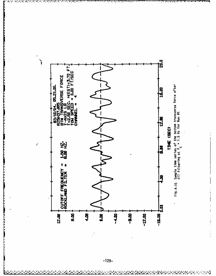
LLI

C C

I 0

0 00

I --

t@3

Io IVC

-129-

C3 u

(A.C

C-- 4j 4*q-1

ZL>

I~~4 r.E

ca,

C.) OUm

ca, C6

Itol

-130-a

C)b

ZLL.Gw

U.

'41

L. 0

E cn

4A w

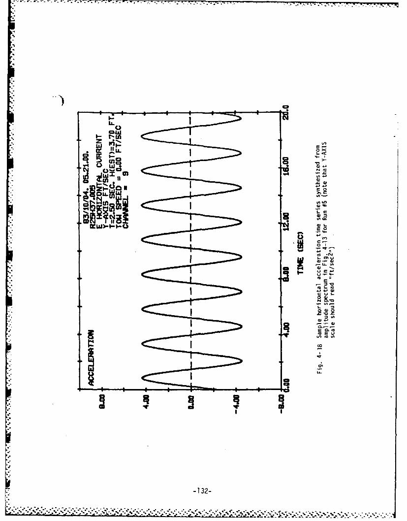
* ca

WIn I N00

w 0J

~OLLW@>

: 0

d- r --

4.) 4.) W

.r_ u -

oGO

C-C

m - ui

VI) Ma CA

cio

-132-

. o'pImooP

C--0

4J 4-V

0

-CC-'s

CC2

LA.

rC

* b

.4133

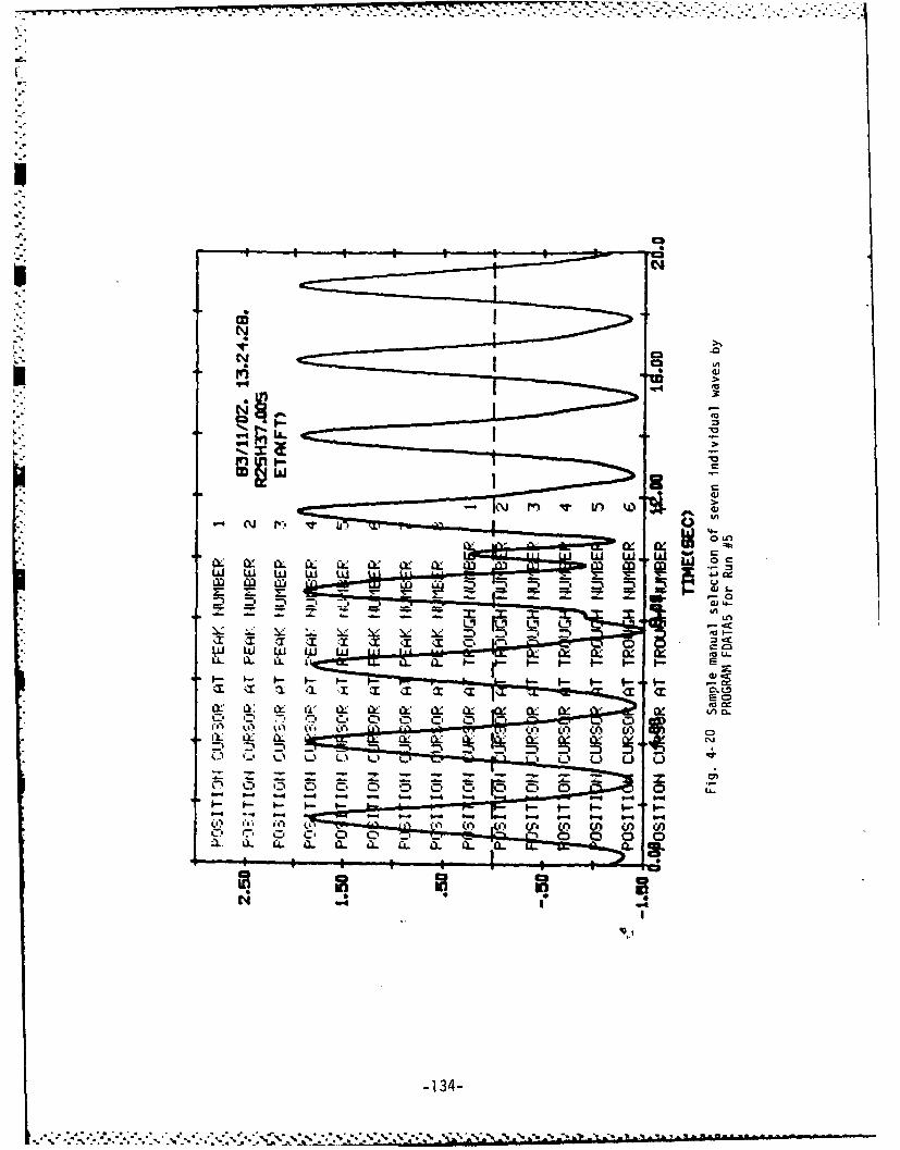
C3F 3l

LW

o a

-~i L CL CL w L w L w l) w.-

n

CL fLC LC

~~a)~L Cli A .

-7: C- C) - - -o -. -

k- 15 3- 3- ro

v. ;71 M ~aa ( f, (A ( A.~ )U (0C., r. C. C o -a.a .a. a_ a. X. CL

-134-

100

oJ

LLJ% ~ >

ZJ'-

w~I-

(U Lj-

EO

faai

-735-

>1

,A in n .0ID 4 W

CJ C -

cm

-1 4- 'o

S-. 4J U

.5. S- uC .

4.-~

w E

CL136-

4- ~ ~ L to 4A - .4

ca ~ e mrCC3P cmC

m -,

to A 9 'sin.

nU?-4 u

a -

C2,inn ca

04-4)-

0-U

a~ 'a-

S--aa--

00

'"4 'lii

Li.00

-137-

*11

u w9Rt

a wa -4

- 0A

a= Q

C~j en

* "1Li (

v~ 0 M LOoenn

A-l

_____ _____ _____ __ U

-138-

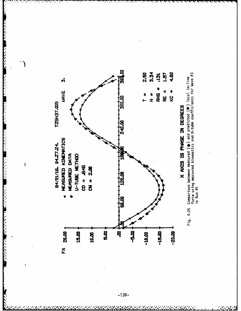
R- W. ' -- -- -- .. ,0 . .LiI II I U

Iw 0

. 4-

! ,E

-341

,-,

M1 U 4

U24-

OC

IL

-139-

0

9~0)-5, cm

0 - 1

0u u

LA

.. C

-140-

III ~ a,

0 v

'-

C-

itE 0

°3 w 0 4

C-=

iu

4-

-14 =-

0-- 4 L-

L-

c~ 0fau

S0i

aja

cl C3

'iioI4

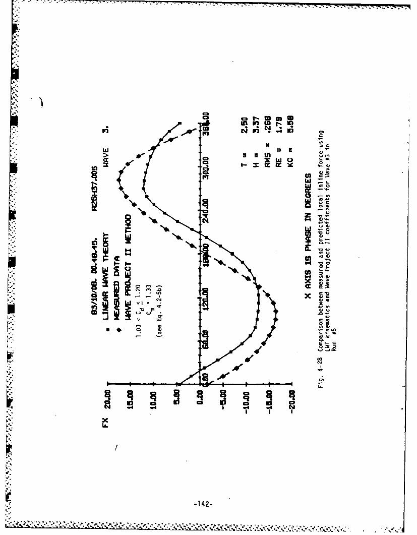
C3 ca.

in~~i 0 WC! ~4

4iL

C3 s- 4-9 ))'I'-

l--4-

i

-142

4A A

* d '.3 . 0

(* *~* ,-- * . * - * 0

p%3

N wu

%" II

cac

-

V u

S .- 4-

73

4- 4A

2

cil

cac

* In

L

-143-

caa

C33

U)a-C3

>1

Eu >

S 4.1 U

3.3

-1-..................... ~a - -. .- * tc

p

in m t

innIL It =, o 0o

*- L

C2C

• -' -

aia'00) to

4J 0CU .- *-0 41'

en

o 4

-145-

in~ in t- toC

44

UUII UW

aIr ZW

C2.

a ~ .~09

0)*

> 4-

IA 3fl.4A

0 c4. .

- 4.-

Eu

.%A 4J)

LC.)

S U

4en

ca

-146-

-%

ca c

Ln W) ,q -1 = I,

, X 4-..-

G4-

ww

,-

* 3

I- go

• IS

) 3

u M

00

'" V

N 0. E

4,J

C-) &-

," x

-147-

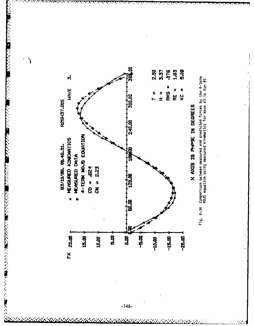
iniU P) a,

," °U

• °C

in N) ,-

>0 t

C C3 w.4-

Euin .

W u >

00

--

0 to

.: !,- -148

",to

0 A

oC

wq

*04--ccz A

41U

Q. S- ED'a~ 4-c;)

~SG

X C-a

0CM~11Lflen

x

P.A

* -149-

> n U)

2CIna.n 0 >

o04- 40

9. .

tU 4-

4-c

.0.IL t0 C7

4CM3

LL 0

C33

CL -

V4

C340-

C2,cm R 9

R W-

W40

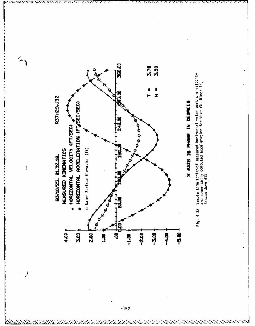
F1W1u

I UIT

104-

po 4-

I-~S - u

4J %- 06

to0

iCn U UNL X4 4 ,C'4

4.-

a, 0. V4- E z

I/ 0 00

-152-

% .. % 5. Ce *e .. e* . .r . s.P

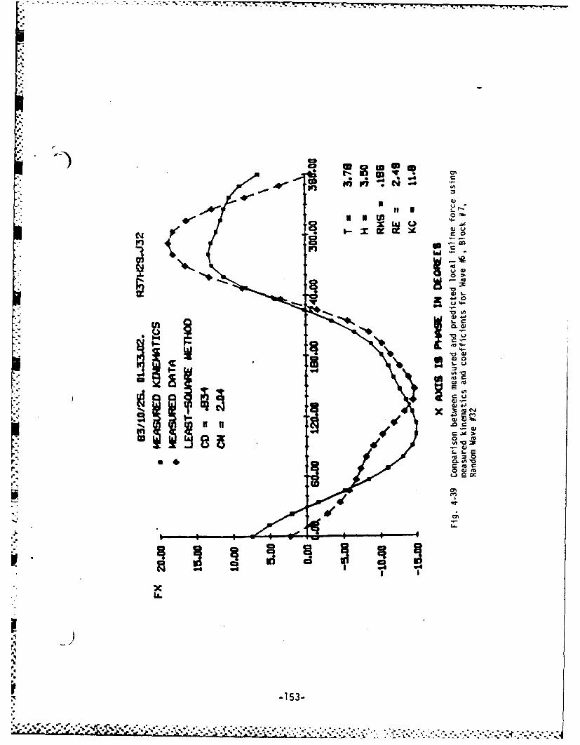
i to

CY 0

I4 0

.W -

- Eu

V

Gil

d)

V) 41

W 34I)

U) c

or= IV to

0'3

--153-

5I ",, - . ;_ ' _- :-;.;,a-'.:-..., .< ¢'-. .'...-... -'.--. .. .. . .

/

w 0,.

C

--

:9 U

,00

;- 154-U 4

L.m

~IIS

0 to

LA4-

09-

LL@3

-154-,

C .4

-)

4J0

-0

-4-

U L

.P- -c

0". .

3 Wm

-156-

GJ2C

9-4- U

N cc

in 0 .

0~ 4.)

lD C

. . .to

C4

jw -8

,15 -,

, .,.[- , ,,, ._,,, .,,,- _ ,v .- . .. ",,,u.,, -% ... .a /4 % ., 2 ;.,,,", %..,,./-A .' o".-l _. .- . _,.',- . .

in a

. .dm .- m'rm .

' 4-

o-°Ug

'06'

OCj

4j oc

W -

('a M-

Fo- ;0.

v50 caW.. . - 0

. . .-.

"'a

v- 7 11 *. T. 77 * OP

A A i 5- 1..L €,

3 q 4- 0

in *IWO C xw 0 - a

9

C.

-158-

MU uS. -)c

4) m

-158A

* * * * * * *~~~ * cmr

** A A ~~~~~~Cl IV .~ S~ ~* ~>

LL. -vv-v.-

A-Abe

IIf pUul

mmC3-C3-

S-0

UC u

- to-

4-)

.0-

LL.

-159-

Z**x* Z!!:* ::. - : .

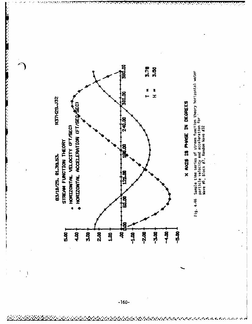
-- T-61

It i

* 1o-K

0~ inLa

4.)

o

41 u

-~~4 4.)

-~w u

S >,

-160-

.~~ ~ AA ,f! C a)

(a >

-.0 0E,

r-. -d- ,

*" -1- -

,0"0

.0 4ea a

J a -o

"C2 - , 0.)

c-'

3o 0

X) ccu

..

_ ",x

4s t- in

00

C.3

90 Cj

CL W

-u 1 0

EU4k

a) )

c >U

( U S-

0)W J0

cac

-162-w

U C

-. 44

* ou

NQE 4-

xwuC3 IlC

S- fa

M.E >"Dww

W4aG

*0 >

'4 E c -m

41ijII. 4- W J

.6.4 -0 I4. 0a n. L9 .

LE'-

'U a:0"0

-163-

V- 0*---- WI P1F1:N. A

*-7 U

cm .0

,cm~ 4w > CI

'0 4- 4,

L 4)

4) S- W

la

03

.00

LL.

-164-

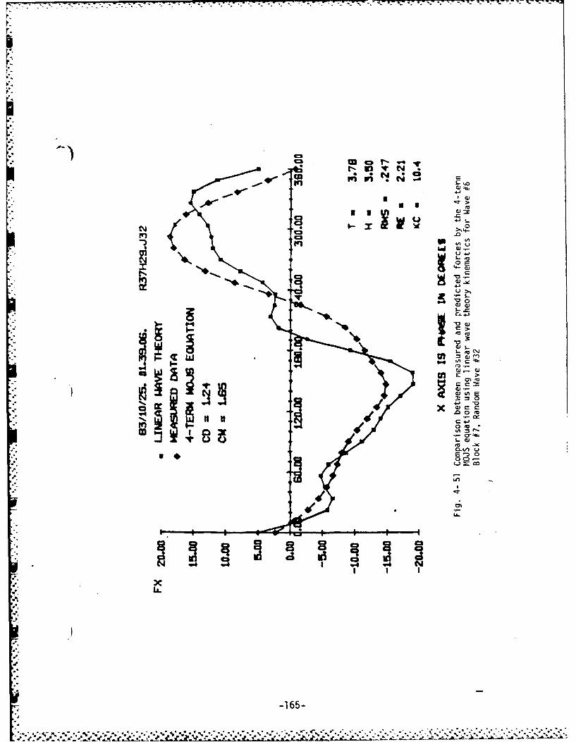
"-C3

li.. I-- ..,

oN

"0 E4- W

UC

S- €' S -ooJ 4v

"" 0 C "

U >M~ 0

.-. ~~ M , GL.

a4'1 0

oo

--165-

%C"i!; o

• . , , ., . . . .' • -, . ,', ,.'-. .'..-r. -. ,',, -" :-" ."'.."-.. . ''.'. %.''..'''..'%' ''..-'-. "'[. "-"-"-.; "-"." .",'-"-',-. % -. %,'.'-.-.-, ,"."."."-..-',,

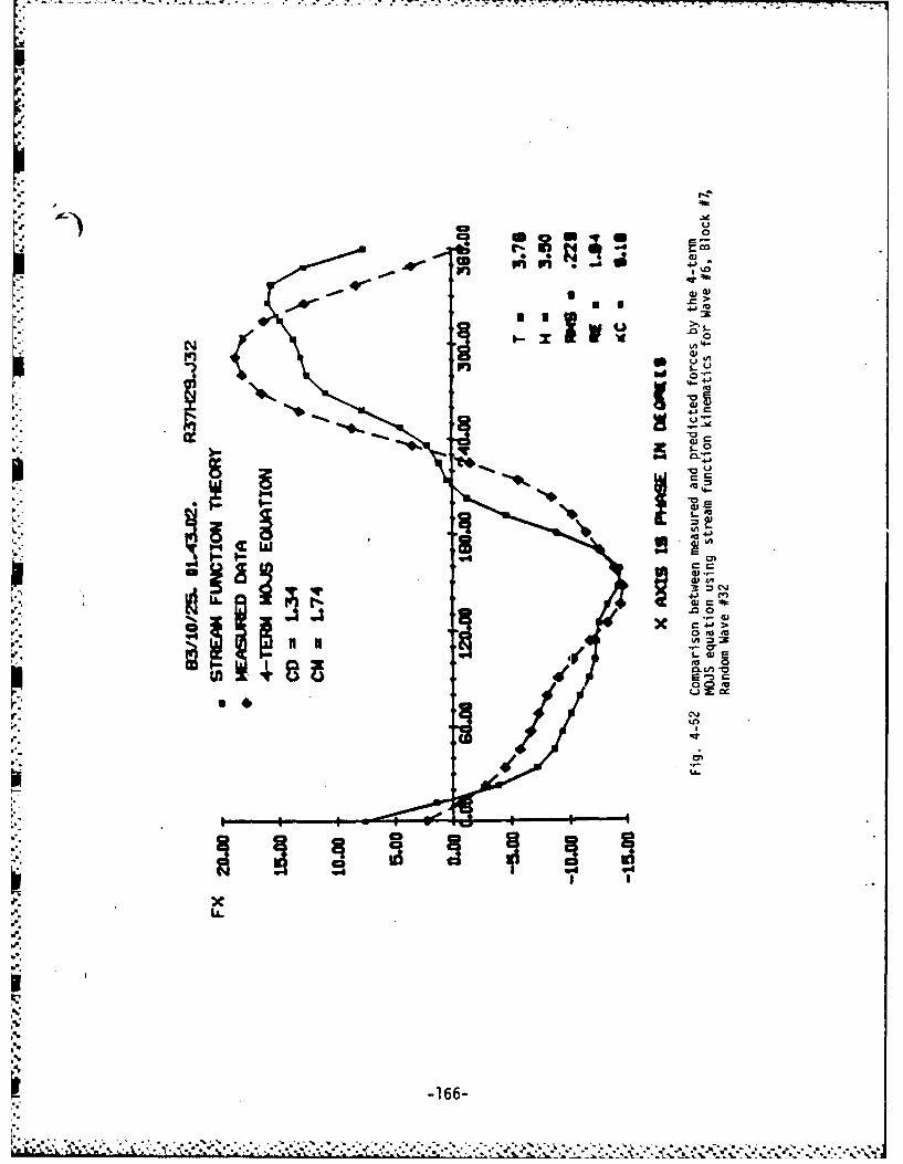
I >0

C3~

(U*

q ,-z,,I.0

8 0J

X>

06'

4.)

.61

Itd4

U. -c66-

0

I,

-. 166-

00

V. - 0 4

LL

11 < wL o0 c;

0 0 w CL

0

x0 1

j<i 0 i10 L. >

o 0L

0 0L w 0r x >0 03 <0

N- -X-j n 0 0,3: I C;U

I..N r.0

('JZI.0

Z x.

- 07

I'C;

0 dL *J- ~ p.- -- p A ~ -

00

00

Ln U)

CLC

00 *

~ - N

U~az 0

NW z

>'Ll0 4.1

< w uwU N

0< -w-

-0 31 L

o 03 <U--) '> m w4

0 0i 0 0 (0 N

It i 0 -' <0U

ww

-168

4-z 0zN

0--4 U

Lnw >zn a

7- EA0 c

0 wL w .0

m 0

<

-i w

(OZ o *xx~0 L

ZN xL

W~h00

0 c

0 0 0 0 0 06 -

-169-

404

U. 13

K 0

-Lfl ~4- J

w -4- 4A

4J-

13 - *,oa

00

w C) -

>1 a tic>0 aa CT<0 t9

0 C

CD

-170-

-

NN41

I- -l

IIc aj< 0>

w caz

0~ '4-

U) C) 4J 1> C>aa~4

C) V ()

N LW

0

Wl 0CLf

CT) -~ La O -C L * ~

E

-71-

-. ; 7. 7. - * .

d3.

wI C\J 4- S.

o ca

ztu c

IL

00(n -n 00

co 4- L

I 0'a4-

C0 cL. =

0v>

LL.

cV) CM 0 % O col r- coN 4t c

06 0 0 a

-172-

~ * : .~* ~ **-** ~ 9- *

. . ..- -- *u-''& 5 n__U__ ___ __

ilfljI N-4W

o 4o

-r-

IJ c

(A 4-

4) -

< o-,

coo

--

LON

U) aJ

W ) 00

U

W CD

>04T

1-4uN 1

cv 173-

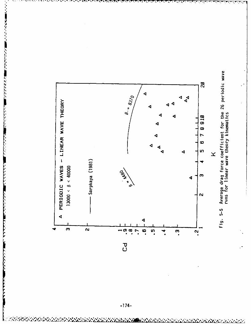
CC-,

N~

co03c4

z =

I--

C)l o. 4- t

cn C

J.0,

0 .9-M

C)JCz >

IQ

LO

03 CC- t- o nm ,

Eu 4u

V Eu O174-

- - - .~rL

c\J

1-4 04If 0 > -

u 4- -c

ci 4.. 3

ILL

-n 44-)

) m to

CL.

0 >3" 0

C)'

"t m NC)C taw-- uO Lr * c CY

-175-

LL

(A S

Ln

cv -

u0

a LA) =L

V-S4- (D

(nn

w 4-1..

* 00* -00

f l i 04_

EU 4-v=

ca C *4.4.

V EUl L.

00qzo

13W

(T) c'J .0)WV CD IfCO ) "i m1 N~

E

-176-

eod

p~

U-)-

II 0-

4- r-

0>

wz 4-

CD W

0n ciiO 04w CV)'4-

> 0)Vo

<>6 6'

3: ca 40

v CL

<oo

m'Cl N~ l)W C o t) . CO(7"t C) Nl

0 0

-177-

wz >.

C~j 3: r

0 .~ 7

o --

LLJ 4-

Zo (Aw S*-

Li. 4-u

C) (a

<cn S-o -I--

Z 0DCDU

to 'UONJ

wo ..

<cV OL )C t OU) V c ~

-178-

N- -

cn 0)

Ua 4--C .-0

I - 4r - .WL 0i v) s- ,.v

ir4 -)

.- w

Coo

C4. u

w ) ..- a>-

>1 v. 01>

CY) CD

LGJO

o n (MC I CnE4 c \

0T

-179-

s- 00

> u~

4-= ea.

4-

w 20*-z- -U .J >1

- 4- 000 4-4.)

- 0 54-40,

C/) (U -

00 C

s- (u

C)t

IV Cn (V 0.) CO t- 0 t n "e cv~

-180-

------------ ~

N -. ' ~ '' ~ - .- LA

C-

0 .Y - 41

u > T

o 4 .o

-= 3.-j

00 30

C,w C., f

> - ' .- L

Ga 4-

S-.

( 0 -D S..z C S 0 ) -

I-r U ~ 3 Dt DU 4 nNU

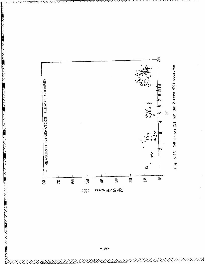
444

C3C

0) c E

r- 41

-)

44

W 444-Y

z t

LI

CD CC Ir Il -.

X cN- CO N 6 M

-182-

04 0

4-

u

0~0

Ld4 4$)

4 4O

~4~j~g5Mt

x - 4 C-1834

-~~4 4:...

4444

4 c

4 444

44

I.-

00

(-I--S

LLI 4in 4 %

W7. X4-

-184-

44

D4~ 44

C3 44

j444 4co -

44

1> 42

LdL

LLL

I zJ

ea

-185-

a.r

10)

Ldd

< -)

U 4 44 0

-44 .o

cr) .-LU0

>= 4

< -

3tw 1l

LI 4IY44

_j4

tm M m m tm m U3 .

CD ~~~ 44Lnm

M X ~uj N 4

w186

-.--.---- , ~ 7 7,-----

C 4

w

*1- m44 o\

w t> J-

4MI M'4mts

co Lr)

X 4-l 4

--C

-1~Wft

z0

LLL

F- LAci'4

tm m m c

ro 44 LO "i

4M mi sv

444L

W~ 4A

U -L-

-1891

j4C~j

.- 00

444-)

44 4 44

-190-

II

44--

00I -0)

C, -ww

'-4-

CD r c - ~

M0 (iiz/s~

0)

t'. 4t's

0 4

44

1-

4 4 0

4ED cm4 to, S

co in04 -

M XCILJ/sC4:

4 192-

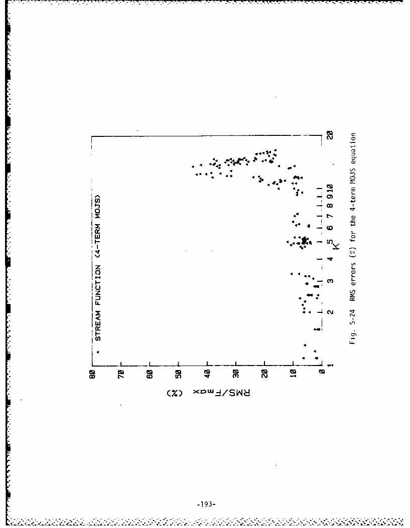
'04 V0

44 m4*4

cy

44*?7 444

4 44- 4~co

L-C

LL.

<0

-193-

AD-AiS? 722 HIGH REYNOLDS NUMBER HAVE FORCE INVESTIGATION IN A NAVE 3fFLUME(U) OREGON STATE UNIV CORVALLIS DEPT OF CIVILENGINEERING R T HUDSPETH ET AL. MAR 85 NCEL-CR-95 864

UNCLASSIFIED N62474-82-C-98295 F/0 26/4 NllEE~hEEEEEEEE

i

Ohl

110

1*21111 Sl.

NATIONAL BUREAU OF STANDARDSMCocOy f LUnMf TEST CHART

4%

4%%

% %

9. . ' . . '. " , • *. " , " , *. ' , ', _" . " .. .'-'-'-.:''- -" , - . - * • . "- . - - .'

IS. '',,* ",, ,. , , *,". ... *,._,- .'.":.:.,...,:-.'-".:,' .. . .-,... ..... ,., ,?.. .; '. ''" ..... .","... .

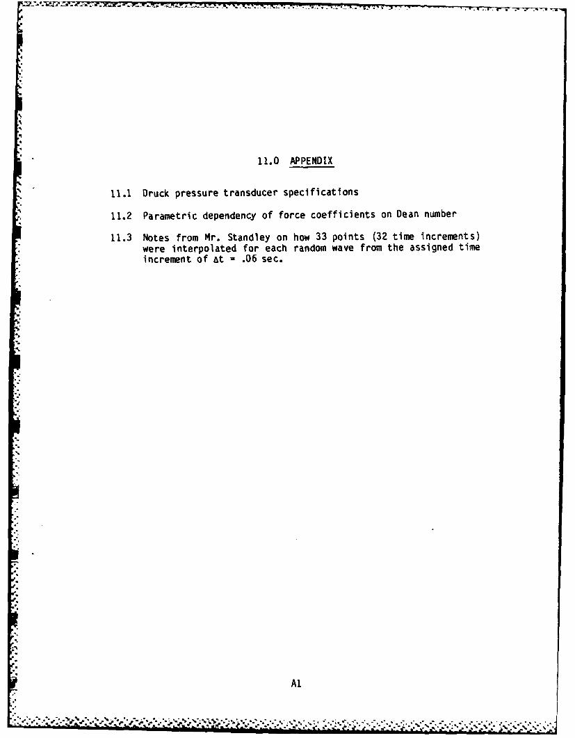
11.0 APPENDIX

11.1 Druck pressure transducer specifications

11.2 Parametric dependency of force coefficients on Dean number

11.3 Notes from Mr. Standley on how 33 points (32 time increments)were interpolated for each random wave from the assigned timeincrement of &t = .06 sec.

"A.

o?

,.

0'" ."' ... ," " " '-, ," ' ." ". "", '", w .. , .".".".",,. : .-; .-. ' - -. ..-. -. - . . .

.. .. .' 'i ' , ' m - , %- .t ',",.. . ..",, > . " .." -, . " ..:' '... ' :"'...'.Al. .

• -- .m im m 0 m **± * a - a , - • m

APPENDIX 11.1

DRUCK PRESSURE TRANSDUCER SPECIFICATIONS

A

.4n-

A3

. *<a - -A : - -

D Druck Limited

- 8 Fir Tree Lane GrobyLeicestershire LEG OFH EnglandTelephone Leicester (0533) 878551Telex 341743

.

Thousands of Druck pressure transducers are being The construction of the transducer is completed usingused throughout the world in applications where high microcircuit, alloying and bonding techniques, andaccuracy and reliability are of importance, and the electron beam welding. The ancillary electronicPDCR 10 series has been designed more specifically package to give good temperature compensation,for the industrial user following years of operation of rationlisation or amplification, is encapsulated. Thethe PDCR 22 and PDCR 32 transducers in mainly complete transducer, having effectively no movingaerospace environments requiring maximum per- parts and being both mechanicalv and electronicallyformance with regard to weight, reliability and extremely rugged, is therefore ideally suited toaccuracy. The PDCR 10 is an extremely rugged industrial environments of extreme vibration, shocktransducer and operational ratings such as shock, or other external effects.vibration and overload are extremely high as is usual Many pressure fittings are available as standard and thewith microcircuit devices. transducer case is of stainless steel and titanium. A

Pressure ranges extend from 1 to 5000 psi, gauge, polychloroprene cable is sealed into the body with asealed gauge or differential. The standard output of heat shrink boot. The integrity of the cable outlet seals1 OOmV with 10 Volts excitation is available on most is such that the entire transducer could be immersedpressure ranges whilst still retaining high linearity and to depths of at least 300 metres.hysteresis accuracy (:0.1% 5.S.L) and high overload Different versions are available which include bore holecapability. transducers suitable for continuous immersion in salt

A silicon strain gauge bridge is diffused into a single or high mineral water. and also transducers are available

crystal silicon diaphragm using microcircuit techniques with a 2000 ohm resistance bridge network whichand so it is effectively atomically bonded, and this makes them suitable to operate with two wire 'mA'feature, combined with the fact that there is no transmitter electronics.measurable hysteresis in such diaohragm material, Also current outputs can be sufficient to drive metersmakes an excellent fundamental sensing element. The and galvanometers of oscllograoh recorders directly.gauge factors of the four silicon gauges areapproximately 50 times those of conventional wirestrain gauges so that the output can be relatively highwhilst still retaining a high overload.

A4

.;... : ...,-, .......;.-, . .,_-.... ,_. , ... ... .. _,, ,.. ..,,.. .. .... " 4 ..,. .-' : "... .: , '> '-,'. ;-

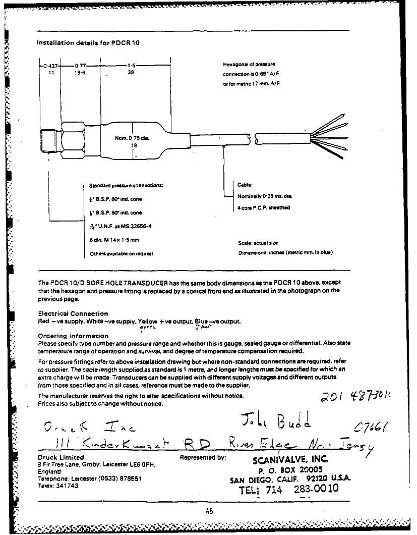
Installation details for POCR 10

0-437 -0-77 1.5 Hexagonal of pressure

11 19"6 38 connection is 0.69 A/F

or for metric 17 mm. A/F

I' B.S.P. 60* ind. cone Nominally 02S ins. dia.

V S..P. 0* nd. one4 core P. C.P. sheathed":: k"~~ 8.S.P. 60O intl. cone PCP

1 " U.N.F. as MS.33656-4

6 din.Ml14x 1 5 mm Scale: actual size

Others available on request Dimensions: inches (metric mm. in blue)

The PDCR. 10/D BORE HOLE TRANSDUCER has the same body dimensions as the PDCR 10 above, exceptthat the hexagon and pressure fitting is replaced by a conical front end as illustrated in the photograph on theprevious page.

Electrical ConnectionRed - ve supply, White -ye supply, Yellow + ve output. Blue -ve output.

• . Ordering informationPlease specify type number and pressure range and whether this is gauge, sealed gauge or differential. Also statetemperature range of operation and survival, and degree of temperature compensation required.

For pressure fittings refer to above installation drawing but where non-standard connections are required, referto supplier. The cable length supplied.as standard is 1 metre. and longer lengths must be specified for which anextra charge will be made. Transducers can be supplied with different supply voltages and different outputsfrom those specified and in all cases, reference must be made to the supplier.

The manufacturer reserves the right to alter specifications without notice. o t 7-o0* Prices also subject to change without notice.

Druck Limited Represented by: C8 Fir Tree Lane. Groby, Leicester LE6 OFH. SCANIVALVE, IN.

England p. o. BOX 20005* Telephone: Leicester (0533) 878551 SAN DIEGO, CALIF. 92120 U.$JLTelex: 341743 TEL. 714 283.0010

A5,~~~~~~~~~~~~~~.....-........'........ .. .... .*.'..... X ................... ',• ,,. .... ..... ..... ... .......- .

.' . - . -. - .,.,w - - -4* . -%.' %= % i" ** _i : $ f % J ' '.I * " .' * I

Bore Hole and Depth MeasurementTransducer PDCR 1O/DA version of the POCR 10 has been specificallydesigned for depth measurement in bore holes,reservoirs, the sea and many other applications. It hasthe electrical specifications outlined on the oppositepage, but a special front end has been designedwhich makes it ideal for dropping down small borepipes, and discourages the ingress of ptirticles. Extraintegrity has been built into the cable seal, andcombines encapsulation, 0 ring seals and a heat shrinkboot. The pressure ranges are vented gauge for thelower depths but sealed gauge versions are normallyrecommended for depths above about 150 feet.High accuracy versions are available with a linearityand hysteresis combined of less than ± 0.06% B.S.Land temperature compensation from -2°C to + 30*Cof better than 0-01 %/ oC for both zero and span shifts.

Options also being manufactured (Technical note 5) and theFor many years we have specialised in producing more standard ones require a power supply of -- 12.0,pressure transducers based on the use of an integrated -12 Volts and give output voltages of up to 5 Volts,silicon strain gauge diaphragm and have solved many with a low output impedance. Again, the generaldifferent pressure measuring and recording problems, performance in terms of accuracy and temperature, areThree such transducers are a differential version, an the same as outlined for the PDCR 10, although wideramplifier transducer and a flush mounting transducer, temperature ranges and higher accuracies areand these are briefly mentioned below, available.

The PDCR 1 OL DIFFERENTIALTRANSDUCER The FLUSH MOUNTING PRESSURETRANSUDCER,(Technical note 4) has been developed to fulfil special PDCR 50 (Technical note 6) has a 0-5 ins. diameter

* applications measuring low differential pressure at front end and a flange which enables it to be mounteddifferent line pressures where high accuracy, small size into tanks and other containers such that the sensingand fast response are important. These transducers have diaphragm is flush with the wail, and hence gives fastelectron beam welded pressure connectors at each end response and accurate measurements withoutand a side entry cable. The current models are suitable disturbing the flow pattern. These transducers arefor liquid on the positive side and dry, non-corrosive already proving extremely useful in marine modelgas on the negative side. and measurements so far testing, general flow research and the processhave been limited to 1000 psi static pressures, although industries.other types are being developed. The zero and These are just a few of the transducers that we havesensitivity change for increasing line pressure is often manufactured over the years to fulfil specificnegiigible and the linearity and hysteresis in the requirements, so therefore, if you have pressurenegative direction, as in the positive direction, is measuring or recording problems, it is suggested thatextremely low. you contact us. since we may already have solved yourTransducers containing I NTEG RAL AM PLI Fl ERS are particular problem.

A6

Pressure Range& Sensitivity Setting

±1,2.5, 54, 50,100, 150, 250,500,1000,1500, ± 3mV.2500, 3500,5000. lbsf/in (p.s.i.). More accurate settings of zero and span are available

S.I. units: 1 0N/m2 (bars) 0 to 6.895 kN/m' through for applications where interchangeability is important.

to 3.447 M N/ma. Please refer to supplier.

Intermediate ranges are available on request.

Operational Temperature Range

-20°C to + 80°C standard but this temperature rangeOperational Mode can be extended.

Gauge, sealed gauge or differential.

Temperature Effects

Overpressure Any 1 00°C or 50°C temperature band to be specified.

400% with negligible calibration change and higher Temperature error band of = 0.5% over 50'Coverload capability is available especially in lower or temperature error band of - 1.5% over 00C.ranges. For higher ratings please specify. Better temperature compensation and/or a wider

temperature range is available on request. Please referto supplier.

Pressure Media

Plus side, fluids compatible with quartz, titanium, andsilicon dioxide. Natural Frequency

Typical 5000 p Hz where p is full range pressure in psi.

Input and Output Impedance

Nominally 1000 ohms. Acceleration Sensitivity

For optional 2000 ohms refer to supplier. 0.002% FSO/g for 5 psi decreasing to 0.00015%FSO/g for 1000 psi.

Excitation10 Volts d.c. regulated. For a.c. excitation please specify. Shock

1 OOOg for 1 ms. in each of three mutually perpendicularaxes will not affect calibration.

Output

25mV for 1 psi30mV for 2.5 psi Weight6OmV for 5 psi Approx. 140 gms.

1 OOmV for 10 psi and above

Load impedance for quoted performance should begreater than 100 Kohms. For lower load impedances Electrical Connectionplease specify. Integral sealed cable assembly: standard length I metre

and other lengths to order.

Resolution

Infinite. Mechanical outline and ordering informationSee back page.

Combined Non-linearity Hysteresis

±0.1% B.S.L

Zero Offsett 3mV. A7

* APPENDIX 11.2

PARAMETRIC DEPENDENCY OF FORCE COEFFICIENTS ON DEAN NUMBER

A9

.

Ocean Wave Data. Dean and Aagaard (1969) used measured

pressure forces from a prototype offshore oil platform and a least-S.

squares regression analysis with theoretical nonlinear water

particle kinematics computed by the stream function theory to com-

pute Cd, Cm. They found that the drag coefficient varied with

Reynolds number and that the inertia coefficient was essentially a

constant. The Dean and Aagaard regression analysis illustrates the

parametric dependence of the coefficients and explains some of the

scatter observed by various investigators.

Dean and Aagaard (1969) computed CD , CI from a least squares

fit to the measured forces by minimizing the following mean square

error:

21 N 2= n {Fm(n) -Fp (n)) (1)

n

Minimizing this mean square error requires that

2 2ac = 0 and = 0 (2)m d

Equation 1 for the mean square error may be expanded into a general

equation for a quadratic surface of second-degree with an origin

which has been translated and rotated. The coefficients of the

independent variables include products of the wave field kinematics

and measured forces and determine whether or not the data are well

conditioned or ill conditioned for determining true minima (Dean,

1976).

A10

_". . ... : .......- .. .-...... .....

"q" o " , ." . ,,- ' "o • I " - -- -q • . . "' ,, . .. ,. , .. " . . ' , .. ,. , - .,% ; . %, ", . b "% - - . . . ,. m. c - " . .. - .. -. . - .. - . . . . . .- , . . . .. .I P.' p *" ' --- .. ...I.*.*

a

Expanding the mean square error yields the following equation

for a quadratic error surface:

<u > + +Cm <uu>+u2>) (Cm

-2 Cdp <F m ulul>- 2 (Cm 0- )<FmD> = <F2> (3)

in which the temporal averaging operator <- > is defined

by <. > = 1 . )n" This equation is the general equation for ann )nn=l

ellipse whose origin has been translated and rotated. For data

which are simple harmonic oscillations, the coordinates of the

origin (xo, yo) are given by

x 16) <Fmuu> (4a)xo V <U4>m2 Ty .2) (__L_2 D <Fm> (4b)

pW m

To determine the suitability of the data to resolve the regres-

sion coefficients, Cd, Cm, changes in the minimum values of these

coefficients for a given mean square error are minimized.

For Cm = constant, it may be shown that this minimization of

the changes in the minimum values gives

2C 2 (2 min]1/2[i - e) m6,u4>J1/2 (5a)

and for Cd = constant:

Ev"2 2 )min] I1 2

6 C = 4 1 i i(bm p-O - (2>]i 2 (5b)

All

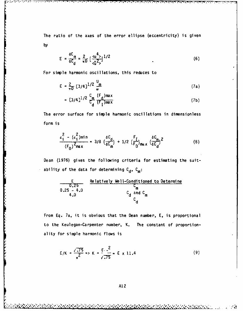
t71

The ratio of the axes of the error ellipse (eccentricity) is given

by

E Cm 2< (6)

For simple harmonic oscillations, this reduces to

E = 2 [3/4]1/2 Um (7a)

= [3/4]1/2 Cm (Fd)max (7b)d- (F )max

The error surface for simple harmonic oscillations in dimensionless

form is

2 2= )min 3/8 ( -C) + 1/2 ( F )m x 6- M2 (8)

(FD)Zmax m D d

Dean (1976) gives the following criteria for estimating the suit-

ability of the data for determining Cd, Cm:

E Relatively Well-Conditioned to Determine0.25 C

0.25 - 4.0 m

4.0 Cd and CmCd

From Eq. 7a, it is obvious that the Dean number, E, is proportional

to the Keulegan-Carpenter number, K. The constant of proportion-

ality for simple harmonic flows is

/K7"K5 E. 2

E/K 2 > K - - - E x 11.4 (9)

A12

.* *q * * .-*.T .ES -~~

APPENDIX 11.3

FDATAR

Choose starting peak of desired wave.

DT = .06 sec

NP = # of points in original wave profile including both end pointsat spacing of DT

PERIOD = (NP-1)*DT period of desired wave

- j -

0 LAG LAG + NP NFT =128

NFT = # of points to FF[ including desired wave in center

OUTPUT wave must have NN = 33 points

Spacing of output wave (delta-t) = Ir = PERIOD/(NN-1)

*', N = # of spaces in total FFT window at delta-t = TT

FFT the data and filter at 2 Hz since original data were alreadyfiltered at 1.5 Hz

Starting at time = LAG*DT compute NN points using the coefficients

NFLTR-1WAVE(I) = XR(1) + 2.* m XR(m)*cos(2ir*(m-I)*T/(N*TT))

-- XI(m)*sin(2w*(m-i)*f/(N*TT)

where T = (LAG*DT) + TT*(I-1).

A13

- . '. . .

S. .

.''-°'*. ''° .- ''-',."*'-'%". ;-4 "- %..,.-* %.-. V .- '....-................%. * ° %%.,, .-. . ° .,. ... .- -.-1-,

- 4.M. R

w

ww

(1) ~ 0 1.=- 0LL W I.-

12t 0 0 - l

I-- .L Z- WQ.-

WU'LU' =00=.-.-46 0..~ 04 a L m.a.

0" WLL CvL.C (i) ('JWW &X(I. j-'4 W0 .- Co OU)C

%,* - - wC 2 0 kD -W

(* w Z C * -W%,

0 6- 0- LA. J *\ \ x

w - 04 iX 96--

W*Ww - Q(PaW --

0 ~ ~ w ,a OZL

<X '- - \ \C-i

I*~ 0.. CL

bo*I ci.. W IC Lm0 * -ACY. I.' J I I. I * z

( 0 Y0av2' Q)4)UEOD4 M A 0I ~ * .'.*

~ (ILL0.J.~ -' *~0iX..3

W UISC'.L

4Q W ~X . rA14

wi

wUS

CLw C4

cQQ3 4. w L

+W -Oo. W) 4

W wO

x wC'tji -- !

*L .1 X0 cn

W =:x4

~f NW 4

W 4' L-3X -0- LAoI- 4 O9 -

w a. W

~~ 'w

I--- "n Co

)- *

*NL CC'. (.UL *L X

~~~C W~~:%% n -J . ,

% +

0w

00

.- J

5-o

.

,,',

It2 11 a -=i u It

+ Ie. WHO X11

U) .LI ' IZ. U~ ~.. II I I ,,..O

_ a J I i .. I-

I r~~ojN-Di 3i ~

r- -O 45n t5zxN

A16Or-c)

'SI.

" + .- - . " r " "N rai . LU .. . i ' " . .. . .

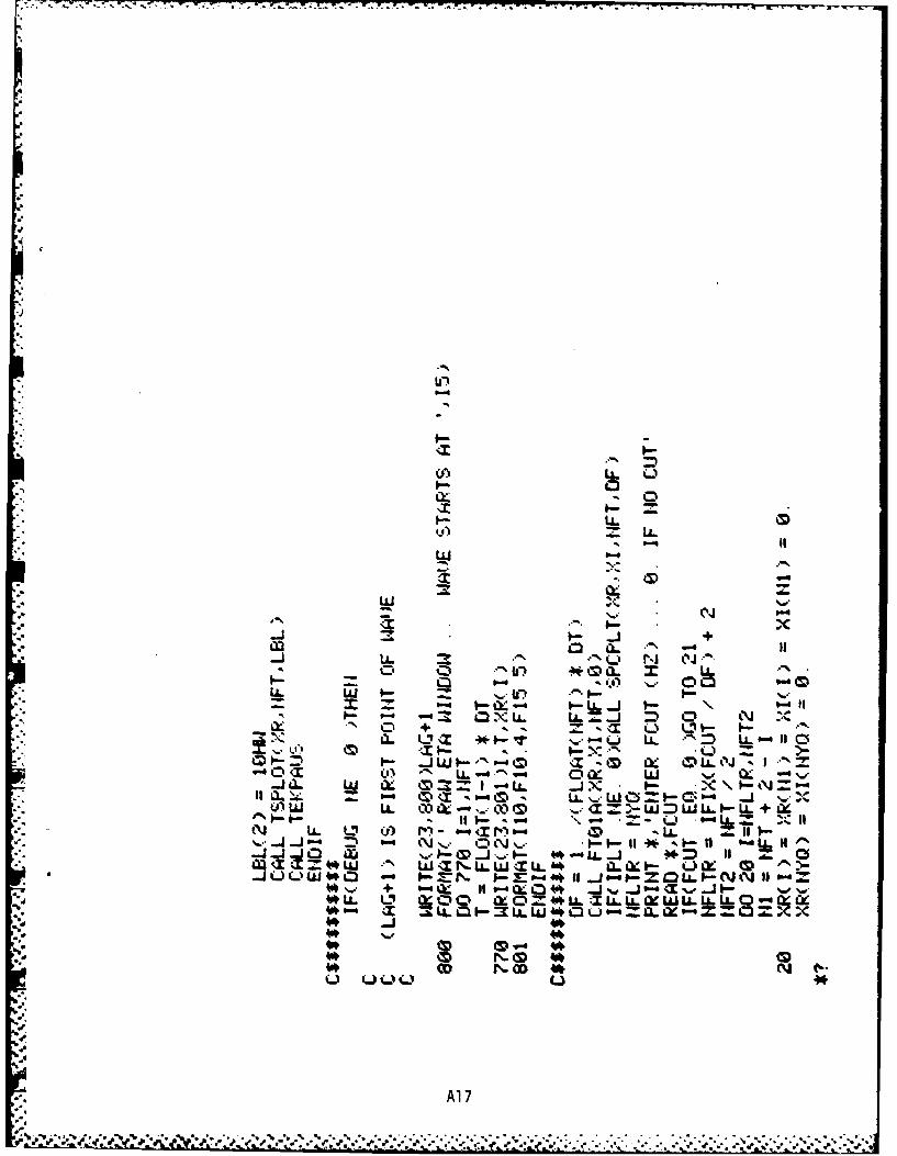
U)

L.

- ) 0L (

LX W- l-LLP.1

.Z . 3

UiL) .L 00 1

-x X =% .-i. I- -_jWI- ,~ 0X~. LiX.".n 0 N ,I--=

.J I'. VZ- iU) I LL I'

CW _j O4*-L LLJ _ - 40\M-It J

L 4II C- a w QZUW L4 kL.. x 0Lx

N LAW LL )r~ 4- 0 &ZOO

:P. D O W~~.~~.4 0-Q Q-r- 9 r J- J~ J -

WL. ~ 00~ 0 U.Z A17.O'

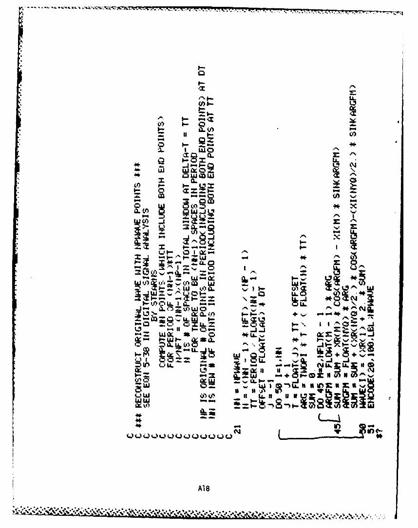
I I LL

_ =-1-0to

I--

IWO

I-- 1 -j *OL17 V., W 0.

L)Dz I:*- ,-#o 0 0)=

"" It - -%" AIQ

- L)L' aI ww0 $- a4. %J.

0. IX

Q- I

w UNb-.i I ~ LII *-

QI- II W

Q))SW II-I. 4U0A

A18B

* U)

CL I

(.Q*w

Z II I25

J+ w I

w C~

M a. W En

Q0 Ix w

+ CD+Ci

w3 m U j 6: C. oI o- - 4(\ 04 4 . f 0 ix w.0O.

g~~~~ Oa - '-- aL Z - ----

+~s- = ~ ~ -40 40

inIf \QlD$~ #*N. ON 4w

L) LL O L) L.~

A19

'I.-I

B

'a

p.

* tE~-a

-a-a

-a-a

P20*, ~~***** S ~

I.. -* 5 5 * 5. *5 .** .5 '**5*** **. * ~ *~** .. * ".~' S

.5 5. *~ S - * .5 ~ *.~ S *5*~~~ J *. * S* *~ *~ 55

~ 5- '.5

un r -

0~ r-)

IT-

LL.

CT

WW

U- CT ~.) CWL

* w

a .. L XXU..

a-

A21

?~~~~~~a. Z ~ ~ ~ S P .. ~*~*~ U.\ *~~~

III

~I

I I

w

II

* I

I,, ,,,

! I'

A23

77-7 . 4r-

4'

:2.

.%e

S..

ii:.gj.

rni

a aa

A24

ml..ml

C %'°%'m . % m

* -' - - - ,%~ * ' % m % % \ j i ~ ' \ m 5 , m ~ m ~ * m

I-'

U.

N

=

I-

a U.

p. wpa t-..pa w

C.-.

a.

paa.

A2 5*...*...*..*.*.*.. .. *..*,*.. .. .-.. ... ... .. ~..............a p

S* a..... ~ -a- -

CM

BI

ci ,

" NCaC

I , !

caa

A26

v - . ' v% ' ''-( - .,x- -, __ * -a. a ,a -. K '.,'A . . . . ..

F,,

A

FILMED//

'

9-85

DTICA p.~% . * ~ ~ ..-- * -

AD-AI57 722 HIGH REYNOLDS NUMBER IdAVE FORCE INVESTIGATION IN A HAVEFLUME(U) OREGON STATE UNIV CORVALLIS DEPT OF CIVILENGINEERING R T HUDSPETH ET AL MAR 85 NCEL-CR-85 "l4

UNCLASSIFIED N62474-82-C-88295 F/G 26/4 NL

Eu....

.1.

1'--

IL251114 11136

MICROCOPY RESOLUTION TEST CHART

NATIONAL BUREAU OF STANDARDS- 1963-A

I

111 I

111i.1 B S

SUPPLEMENTARY

- 9-

INFORMATION

-JSN~jd)t i .INJVdNI IAW1 IV (I liJItiuoI.II ol

DEPARTMENT OF THE NAVYNAVAL CIVIL ENGINEERING LABORATORY

PORT HUENEME, CA 93043 IN REPLY REFER TO

5600

Ser L08/18397 Nov 1985

From: Commanding OfficerF To: Distribution

SubJ: Errata Sheet for CR 85.004, "High Reynolds Number Wave ForceInvestigation in a Wave Flume," by Ocean Engineering Program,Civil Engineering Department, Oregon State University

1. Please insert new pages 27 and 28.

tP.D. TRIEMBy direction

'1%

Rockland Filter

The Rockland filter is a two-pole Butterworth filter. The

filter function is given by

f2 fHRMf0 0 (4.1-14)(if)'+2ifoif+f4 (if)f+42 foif+fI

where fo is the cutoff frequency, f is the signal frequency in Hz,

o, - 0.924, and 02 - 0.700 for the flat decay response. Introducing

a dimensionless frequency ratio, e = f/fo, reduces Eq. 4-14 to

1 1 (4.1-15a)(1-C )+i 1.848c (1-c )+i 1. 4 c

HI(c) . (1-4.5872 c 24) - 1 3.248 (1-e _ (4.1-15b)R (1-4.5872 e¢Z+C 4 )R + 10.55 ¢Z( 1 -. 6 Z+€4 )

The amplitude division factor, IHRI' is

IHRI - L(1+1.415 e 2 +E4)(1-.04 e 2+C4 )J-1/2 (4.1-16a)

and the phase angle, OR, is

0 ' TAN 1 3.248 e(l-s. ) 2 (4.1-16b)

Rm "T "(1-4.5872 C + 4ft

Table 4-3 summarizes the amplitude attenuation and the phase shift

introduced by the Rockland filters in the NCEL data.

Digital Formatting

Exactly ten periods of data were recorded for each of the 21

channels of data measured during the periodic wave tests. These

data were reduced to exactly eight waves and were digitized at a

-27-

sampling interval determined by the deterministic wave period, T,

and the FFT base 211 a 2048 according to

at a 8T/2048 - T/256 (4.1-17)

Each single periodic wave in the eight-wave sequence thus contained

256 data values. This data digitization scheme was required in

order to insure that the data could be FFT filtered as previously

described using an FFT algorithm of base 2. The FFT algorithm was

taken from Bloomfield (1976). Only seven of the eight waves were

actually used in the final data analyses.

The sonic profiler used to record the instantaneous water ele-

vation occasionally suffers from data "drop-outs" or "over-

ranges." These data are identified as "bad-points" and are removed

numerically by linearly interpolating between the good data

values. On rare occasions, these intervals of bad-points are ex-

cessively long and result in forming a fictitious wave (see Wave #4

in Run #5 in Fig. 4-5). These data have been ignored in the data

analyses because there were only two "bad point" waves in the total

of 182 waves recorded. These 256 data points per wave were reduced

to 33 data values (32 time increments) for each individual periodic

wave in the final data analyses for the force coefficients. The

total number of discrete data values digitized for the eight waves

in the 41 periodic runs that are identified in Table 3-13 was

-28-

FILMED

S1-86

I

- TI

p * v4P