LÉVY PROCESSES, STABLE PROCESSES, AND SUBORDINATORS

STEVEN P. LALLEY

1. DEFINITIONS AND EXAMPLES

Definition 1.1. A continuous–time process {Xt = X (t )}t�0 with values in Rd (or, moregenerally, in an abelian topological group G ) is called a Lévy process if (1) its samplepaths are right-continuous and have left limits at every time point t , and (2) it hasstationary, independent increments, that is:

(a) For all 0= t0 < t1 < · · ·< tk , the increments X (ti )�X (ti�1) are independent.(b) For all 0 s t the random variables X (t )� X (s ) and X (t � s )� X (0) have the

same distribution.

The default initial condition is X0 = 0. It can be shown that every process with sta-tionary, independent increments has a version with paths that are right-continuouswith left limits, but this fact won’t be needed in this course. See BREIMAN, Probability,chs. 9, 14 for the proof.

Definition 1.2. A subordinator is a real-valued Lévy process with nondecreasing sam-ple paths. A stable process is a real-valued Lévy process {Xt }t�0 with initial value X0 = 0that satisfies the self-similarity property

(1.1) Xt /t1/↵ D= X1 8 t > 0.

The parameter ↵ is called the exponent of the process.

Example 1.1. The fundamental Lévy processes are the Wiener process and the Poissonprocess. The Poisson process is a subordinator, but is not stable; the Wiener process isstable, with exponent ↵= 2. Any linear combination of independent Lévy processes isagain a Lévy process, so, for instance, if the Wiener process Wt and the Poisson processNt are independent then Wt �Nt is a Lévy process. More important, linear combina-tions of independent Poisson processes are Lévy processes: these are special cases ofwhat are called compound Poisson processes: see sec. 5 below for more. Similarly, ifXt and Yt are independent Lévy processes, then the vector-valued process (Xt , Yt ) is aLévy process.

Example 1.2. Let {Wt }t�0 be a standard Wiener process, and let⌧(a )be the first passagetime to the level a > 0, that is,

(1.2) ⌧(a ) := inf{t : Wt > a }Date: April 12 2007.

1

2 STEVEN P. LALLEY

Then the process {⌧(a )}a�0 is a stable subordinator with exponent↵= 1/2. This followsfrom the strong Markov property of the Wiener process, which implies that the process⌧(a ) has stationary, independent increments, and the Brownian scaling property. (Seesec. 3 below for a discussion of the strong Markov property.) The continuity of Brown-ian paths implies that ⌧(s )is left-continuous with right limits, so it does not satisfy thefirst hypothesis of Definition 1.1; however, the modification

⌧(s ) := limt!s+

⌧(t )

is right-continuous and has left limits, and for each fixed s � 0,

⌧(s ) = ⌧(s ) almost surely.

(EXERCISE: Why?)

Example 1.3. A d�dimensional Wiener process is an Rd�valued process

W (t ) = (W1(t ), W2(t ), . . . , Wd (t ))

whose component Wi (t )are independent standard one-dimensional Wiener processes.Let W (t ) = (X (t ), Y (t )) be a two-dimensional Wiener process, and let ⌧(s ) be the first-passage process for the first coordinate, that is, ⌧(s ) = inf{t : X (t ) > s }. Then the pro-cess {C (s )}s�0 defined by

(1.3) C (s ) := Y (⌧(s ))

is a stable process with exponent 1; it is called the Cauchy process, because its incre-ments have Cauchy distributions. (Like the Brownian first-passage process ⌧(s ), theCauchy process can be modified so as to be right-continuous with left limits.)

Exercise 1.1. (A) Prove that the process C (s ) is stable with exponent 1, using the strongMarkov property of the two-dimensional Wiener process and the Brownian scalingproperty. (B) Check that

exp{i✓Yt � |✓ |Xt }is a continuous (complex-valued) martingale that remains bounded up to time ⌧(s ).Then use the Optional Sampling theorem for bounded continuous martingales (es-sentially, the third Wald identity) to show that

(1.4) E exp{i✓Y (⌧(s ))}= exp{�|✓ |s }.This implies that the distribution of C (s ) is the Cauchy distribution.

Exercise 1.2. Let '(�) be a nondecreasing (or alternatively a continuous) real-valuedfunction of �� 0 that satisfies '(0) = 1 and the functional equation

'(�) ='(m�1/↵)m 8m 2N and8�> 0.

Prove that for some constant �� 0,

'(�) = exp{���↵}.HINT: Start by making the substitution f (r ) ='(r 1/↵).

LÉVY PROCESSES 3

Exercise 1.3. (A) Show that if X (t ) is a stable subordinator with exponent ↵, then forsome constant �� 0,

(1.5) E e ��X (t ) = exp{��t�↵} 8 t ,�> 0.

(B) Similarly, show that if X (t ) is a symmetric stable process with exponent ↵ (heresymmetric means that X (t )has the same distribution as�X (t )), then for some constant�� 0,

(1.6) E e i✓X (t ) = exp{��t |✓ |↵}.Exercise 1.4. (Bochner) Let Yt = Y (t ) be a stable subordinator of exponent ↵, andlet Wt =W (t ) be an independent standard Brownian motion. Use the strong Markovproperty (section 3 below) to show that

(1.7) X (t ) :=W (Y (t ))

is a symmetric stable process of exponent 2↵.

2. INFINITELY DIVISIBLE DISTRIBUTIONS AND CHARACTERISTIC FUNCTIONS

Definition 2.1. A probability distribution F on R is said to be infinitely divisible if forevery integer n � 1 there exist independent, identically distributed random variables{Xn ,i }1in whose sum has distribution F :

(2.1)nX

i=1

Xn ,iD= F.

Proposition 2.1. If {Xt }t�0 is a Lévy process, then for each t > 0 the random variable Xt

has an infinitely divisible distribution. Conversely, if F is an infinitely divisible distri-bution then there is a Lévy process such that X1 has distribution F .

Proof. The first statement is obvious, because by the definition of a Lévy process theincrements X ((k +1)t /n )�X (k t /n ) are independent and identically distributed. Theconverse is quite a bit trickier, and won’t be needed for any other purpose later in thecourse, so I will omit it. ⇤Proposition 2.2. Let Xt = X (t ) be a Lévy process, and for each t � 0 let 't (✓ ) = E e i✓X (t )

be the characteristic function of X (t ). Then there exists a continuous, complex-valuedfunction (✓ ) of ✓ 2R such that for all t � 0 and all ✓ 2R,

(2.2) 't (✓ ) = exp{t (✓ )}.In particular, the function 't (✓ ) has no zeros.

Remark 1. In view of Proposition 2.1, it follows that every infinitely divisible charac-teristic function '(✓ ) has the form '(✓ ) = exp{ (✓ )}, and therefore has no zeros. Infact, though, the usual proof of the converse half of Proposition 2.1 proceeds by firstshowing that infinitely divisible characteristic functions have this form, and then us-ing this to build the Lévy process. For the whole story, see the book Probability by LeoBreiman, chs. 9 and 14.

4 STEVEN P. LALLEY

Proof of Proposition 2.2. The defining property of a Lévy process — that it has station-ary, independent increments — implies that for each fixed ✓ , the characteristic func-tion 't (✓ ) satisfies the multiplication rule

't+s (✓ ) ='t (✓ )'s (✓ ).

Since a Lévy process has right-continuous sample paths, for each fixed argument ✓ thefunction t 7!'t (✓ ) is right-continuous, and in particular, since '0(✓ ) = 1,

limt!0+

't (✓ ) = 1.

But this and the multiplication rule imply that the mapping t 7! 't (✓ ) must also beleft-continuous.

The only continuous functions that satisfy the multiplication rule are the exponen-tial functions e ↵t and the zero function.1 That 't (✓ ) is not identically zero (as a func-tion of t ) follows because t 7!'t (✓ ) is continuous at t = 0, where '0(✓ ) = 1. ⇤Proposition 2.3. Let X (t ) be a subordinator, and for each t � 0 let't (�) = E ��X (t ) be theLaplace transform of X (t ). Then there exists a continuous, nondecreasing, nonnegative,convex function (�) such that for all t � 0 and all �� 0,

(2.3) 't (�) = exp{�t (�)}.The proof is virtually the same as the proof of Proposition 2.2, except for the assertion

that the function (�) is convex, and this follows simply by the second derivative test:with X = X (1),

(�) =� log E e ��X =) 00(�) =E X 2e ��X � (E X e ��X )2

E e ��X.

The function (�) associated with a subordinator has an interesting probabilistic in-terpretation, which will become clear in the discussion of Poisson point processes insec. 5 below.

Proposition 2.2 implies that if Xt is a Lévy process then the characteristic functionE e i✓Xt is continuous in t . This in turn implies that Xs ) Xt as s ! t from the left.(Right-continuity of sample paths implies the stronger assertion that Xs ! Xt almostsurely as s ! t from the right.) The weak convergence can be strengthened:

Proposition 2.4. If {Xs }s�0 is a Lévy process then for each t � 0, the sample path Xs is,with probability 1, continuous at s = t .

Remark 2. Take note of how the statement is quantified! For each t , there is a null seton which the path may fail to be continuous at t . Since there are uncountably manyt , these null sets might add up to something substantial. And indeed for some Lévyprocesses — e.g., the Poisson process — they do.

1Exercise! In fact, the only Lebesgue measurable functions f (t ) that satisfy the addition rule f (t +s ) =f (s ) + f (t ) are the linear functions f (t ) = a + b t : this is a considerably harder exercise.

LÉVY PROCESSES 5

Proof. For each real ✓ , the process Z✓ (s ) := exp{i✓Xs�s (✓ )} is a martingale in s (rela-tive to the natural filtration — see Definition 3.1 below). This is a routine consequenceof the stationary, independent increments property of a Lévy process (exercise). SinceZ✓ (s ) is bounded for s 2 [0, t ], it follows from the martingale convergence theorem that

lims!t�

Z✓ (s ) = Z✓ (t ) almost surely.

This implies that e i✓Xs ! e i✓Xt almost surely as s ! t�, for every fixed ✓ , and thereforealmost surely for every rational ✓ . Therefore, Xs ! Xt . (Explanation: If not, therewould have to be a jump of size 2⇡k/✓ for some integer k , for every rational ✓ . Butthis rules out the possibility of a jump.) ⇤

3. STRONG MARKOV PROPERTY

Definition 3.1. Let {X (t )}t�0 be a Lévy process. The natural filtration associated tothe process is the filtrationF X

t :=�(Xs )st , that is, each��algebraF Xt is the smallest

��algebra with respect to which all of the random variables X (s ), for s t , are mea-surable. An admissible filtration {Ft }t�0 for the process {X (t )}t�0 is a filtration suchthat

(a) F Xt ✓Ft for each t , and

(b) each��algebraFt is independent of the��algebra

(3.1) G Xt :=�(X (t + s )�X (t ))s�0.

For any filtration F= {Ft }t�0, set

(3.2) F1 =�([t�0Ft ),

that is, the smallest��algebra containing all events measurable relative to someFt .

The reason for introducing the notion of an admissible filtration is that it allows in-clusion of events determined by other independent processes. For instance, if X (t )and Y (t ) are independent Wiener processes, as in Example 1.3 above, then the naturalfiltrationF (X ,Y )

t for the vector-valued process (Xt , Yt )will be admissible for each of thecoordinate processes.

Definition 3.2. Let F= {Ft }t�0 be a filtration and let ⌧ be a stopping time relative to F.(Recall that a nonnegative random variable ⌧ is a stopping time relative to a filtrationF if for every t � 0 the event {⌧ t } 2 Ft .) The stopping field F⌧ induced by ⌧ is thecollection of all events A such that for each t � 0,

(3.3) A \ {⌧ t } 2Ft .

Exercise 3.1. (A) Prove that if ⌧ and � are stopping times (relative to the same filtra-tion F) such that � ⌧, thenF� ⇢ F⌧. (B) Check that if ⌧ is a stopping time then foreach n � 1 so is ⌧n = min{k/2n � ⌧}. Moreover, the stopping times ⌧n decrease to⌧. Thus, every stopping time can be approximated from above by stopping times thattake values only in discrete sets.

6 STEVEN P. LALLEY

Theorem 1. (Strong Markov Property I) Let {X (t )}t�0 be a Lévy process andF= {Ft } andadmissible filtration. Suppose that ⌧ is a stopping time relative to F. Define the post-⌧process

(3.4) Y (t ) := X (⌧+ t )�X (⌧).

Then the process {Y (t )}t�0 is independent of F⌧ and identical in law to {X (t )}t�0. Indetail, for every event A 2F⌧, all ti , and all Borel sets Bi ,

P (A \ {Y (ti ) 2 Bi 8 i k}) = P (A)P {X (ti ) 2 Bi 8 i k}(3.5)

= P (A)P {Y (ti ) 2 Bi 8 i k}Theorem 2. (Strong Markov Property II) Suppose in addition to the hypotheses of The-orem 1 that {X ⇤t }t�0 is identical in law to {X (t )}t�0 and is independent of the stoppingfieldF⌧. Define the spliced process

X t := Xt if t < ⌧ and(3.6)

X t := X⌧+X ⇤t�⌧ if t � ⌧.

Then the process X t is also a version of (identical in law to) Xt .

Remark 3. The identity (3.5) is equivalent to the following property: for every k � 1,every bounded continuous function f :Rk !R, and every event A 2F⌧,

E 1A f (Yt1, Yt2

, . . . , Ytk) = P (A)E f (Yt1

, Yt2, . . . , Ytk

)(3.7)

= P (A)E f (Xt1, Xt2

, . . . , Xtk)

This equivalence follows by a standard approximation argument in measure theory(that in essence asserts that indicator functions of Borel events can be arbitrarily wellapproximated in L 1 by bounded continuous functions). See Proposition 7.1 in sec-tion 7 below. Moreover, the identity (3.5) implies that the ��algebrasF⌧ andF Y

1 areindependent. This follows from the⇡�� theorem, because (a) the collection of events{Y (ti ) 2 Bi 8 i k} is a⇡�system; and (b) for any event A 2F⌧, the collection of eventsB for which

P (A \B ) = P (A)P (B )

is a ��system.

Proof of Theorem 1. The strategy is to first prove the result for discrete stopping times,and then to deduce the general case by an approximation argument. First considerthe special case where the stopping time takes values in a countable, discrete set S ={si }i2N, with si < si+1. (Here discrete means that the set S has no limit points in R, thatis, limn!1 sn =1.) If this is the case then for each i the event {⌧ = si } 2 Fsi

, and tocheck (3.5) it suffices to consider events A =G \{⌧= si }where G is a finite intersectionof events X (t j ) 2 Bj for t jsi

. (Why?) For such events A, the equality (3.5) follows easilyfrom the hypothesis that the filtration is admissible and the fact that a Lévy process hasstationary, independent increments (check this!). Thus, the Strong Markov Property I

LÉVY PROCESSES 7

is valid for discrete stopping times, and it follows by the note above that identity (3.7)holds for discrete stopping times.

Now let⌧ be an arbitrary stopping time. Approximate⌧ from above by discrete stop-ping times ⌧n , as in Exercise 3.1. Since the stopping times ⌧n decrease to ⌧, each of thestopping fieldsF⌧n

containsF⌧, so if A 2F⌧ then A 2F⌧nfor each n . Consequently, by

the previous paragraph, the equality (3.7) holds when Y (ti ) is replaced by Yn (ti ), whereYn (t ) := X (⌧n + t )�X (⌧n ). But by the right-continuity of sample paths,

limn!1

Yn (t ) = Y (t ) a .s .,

and so if f :Rk !R is a bounded continuous function then

limn!1

f (Yn (t1), Yn (t2), . . . , Yn (tk )) = f (Y (t1), Y (t2), . . . , Y (tk ))

Therefore, by the dominated convergence theorem, (3.7) follows from the fact that itholds when Y is replaced by Yn . ⇤Proof of Theorem 2. This is more subtle than Theorem 1, because a straightforwardattempt to deduce the general case from the special case of discrete stopping timesdoesn’t work. The difficulty is that if one approximates ⌧ from above by ⌧n , as in theproof of Theorem 1, then the process X ⇤t may not be independent of the stopping fieldsF⌧n

(these decrease toF⌧ as n!1).So we’ll take a different tack, based on the optional sampling formula for martin-

gales. To prove the theorem, we must show that the finite-dimensional distributionsof the spliced process X t are the same as those of Xt . For this, it suffices to show thatthe joint characteristic functions agree, that is, for all choices of ✓ j 2R and all times t j ,

E expß

ikX

j=1

✓ j (Xt j+1�Xt j

)™= E expß

ikX

j=1

✓ j (X t j+1� X t j

)™

.

To simplify the exposition, I’ll consider only the case k = 1; the general case can bedone in the same manner. So: the objective is to show that for each ✓ 2 R and eacht > 0,

(3.8) E e i✓Xt = E e i✓ X t .

In proving this, we may assume that the stopping time ⌧ satisfies ⌧ t , because if itdoesn’t we can replace it by the smaller stopping time ⌧^ t . (The stopping fieldF⌧^t iscontained inF⌧, so if the process X ⇤s is independent ofF⌧ then it is also independentof F⌧^t .) The stationary, independent increments property implies that the processZ✓ (s ) := exp{i✓Xs � s (✓ )} is a martingale relative to the filtration Fs , and for eachfixed ✓ this process is bounded for s t . Consequently, the optional sampling formulagives

E e i✓X⌧�⌧ (✓ ) = 1.

Thus, to complete the proof of (3.8) it suffices to show that

(3.9) E (exp{i✓X ⇤(t �⌧)� (t �⌧) (✓ )} |F⌧) = 1.

8 STEVEN P. LALLEY

The proof of (3.9) will also turn on the optional sampling formula, together with thehypothesis that the process X ⇤s is independent ofF⌧. LetF⇤s =�(X ⇤r )rs be the naturalfiltration of X ⇤, and set

Gs =�(F⇤s [F⌧).This is an admissible filtration for the process X ⇤, because X ⇤ is independent ofF⌧. Therandom variable t �⌧ is measurable relative toG0 =F⌧, and so it is (trivially) a stoppingtime relative to the filtration Gs . Because the filtration Gs is admissible for the processX ⇤s , the stationary, independent increments property implies that the process

Z ⇤✓ (s ) := exp{i✓X ⇤s � s (✓ )}is a martingale relative to the filtration Gs , and remains bounded up to time t . Thus,the optional sampling formula (applied with the stopping time t �⌧) implies (3.9). ⇤

4. BLUMENTHAL ZERO-ONE LAW

Theorem 3. (Blumenthal Zero-One Law) Let {X (t )}t�0 be a Lévy process and {F Xt }t�0

its natural filtration. Define the��algebra

(4.1) F X0+ :=\

t>0

F Xt .

ThenF X0+ is a zero-one field, that is, every event A 2F X

0+ has probability zero or one.

Proof. For notational ease, I’ll drop the superscript X from the��algebras. SetF1 =�([t�0Ft ). I claim that for any event A 2F1,

(4.2) E (1A |F0+) = P (A) a.s.

This will imply the theorem, because for any event A 2F0+ it is also the case that

E (1A |F0+) = 1A a.s.,

by the filtering property of conditional expectation. To prove (4.2), it is enough to con-sider cylinder events, that is, events of the form

A =k\

i=1

{X (ti ) 2 Bi } where Bi 2B1.

Let f :Rk !R be a bounded, continuous function, and set

⇠ := f (X (t1), X (t2), . . . , X (tk )) and

⇠n := f (X (t1)�X (1/n ), X (t2)�X (1/n ), . . . , X (tk )�X (1/n )).

To prove the identity (4.2) for cylinder events, it is enough (by Exercise 4.1 below) toprove that for any bounded continuous f :Rk !R,

(4.3) E (⇠ |F0+) = E ⇠.

LÉVY PROCESSES 9

Since the process X (t ) has right-continuous paths, ⇠n ! ⇠ a.s., and the convergence isbounded, because f was assumed to be bounded. Therefore, by the usual dominatedconvergence theorem and the DCT for conditional expectations,

limn!1

E ⇠n = E ⇠ and

limn!1

E (⇠n |F0+) = E (⇠ |F0+) a.s.

Therefore, to prove (4.3) it suffices to show that for each n ,

E (⇠n |F0+) = E ⇠n a.s.

But this follows immediately from the independent increments property, because⇠n isa function of the increments after time 1/n , and so is independent ofF1/n – and hencealso independent ofF0+, since this is contained inF1/n .

⇤Exercise 4.1. Complete the proof above by showing that the identity (4.3) implies theidentity 4.2 for all cylinder events.

Corollary 4.1. If X (t ) is a subordinator with continuous sample paths then there is aconstant C � 0 such that X (t ) =C t a.s.

Proof. According to a basic theorem of real analysis (see, for instance, H. ROYDEN, RealAnalysis, chapter 5), every nondecreasing function is differentiable a.e. Hence, in par-ticular, X (t ) is differentiable in t a.e., with probability one. It follows that X (t ) is dif-ferentiable at t = 0 almost surely, and that the derivative is finite a.s. (See the technicalnote following the proof for further elaboration.) But the derivative

X 0(0) := lim"!0+

X (")"

depends only on the values of the process X (t ) for t in arbitrarily small neighborhoodsof 0, and so it must beF X

0+�measurable. SinceF X0+ is a zero-one field, by Theorem 3, it

follows that the random variable X 0(0) is constant a.s: thus, X 0(0) =C for some constantC � 0.

Existence of a finite derivative C may be restated in equivalent geometric terms asfollows: for any � > 0, the graph of X (t )must lie entirely in the cone bounded by thelines of slope C ±� through the origin, at least for small t > 0. Thus, if we define

T = T1 :=min{t > 0 : X (t )� (C +�)t }=1 if there is no such t

then T > 0 (but possibly infinite) with probability one. Note that T is a stopping time,by path continuity. Moreover, since X (t ) is continuous, by hypothesis, X (T ) = (C +�)Ton the event T <1 and X (t )C t for all t T . Now define inductively

Tk+1 =min{t > 0 : X (t +Tk )�X (Tx )� (C +�)t }=1 if Tk =1 or if no such t exists.;

10 STEVEN P. LALLEY

observe that X (Tk ) = (C +�)Tk on the event Tk <1, for each k , and so X (t ) (C +�)tfor all t Tk . By the Strong Markov Property, the increments Tk+1 � Tk are i.i.d. andstrictly positive. Hence, by the SLLN, Tk ! 1 almost surely as k ! 1, so X (t ) (C + �)t for all t <1. The same argument shows that X (t ) � (C � �)t for all t � 0.Since �> 0 is arbitrary, it follows that X (t ) =C t for all t , with probability one. ⇤Remark 4. The random process X (t ) is actually a function X (t ,!)of two arguments t 2[0,1) and! 2⌦. Consider only those t 2 [0, 1]; then X (t ,!) can be viewed as a singlerandom variable on the product space [0, 1]⇥⌦, endowed with the product probabilitymeasure Lebesgue⇥P . The set of all pairs (t ,!) for which the derivative X 0(t ) exists isproduct measurable (why?). By the differentiation theorem quoted above, for P�a.s. !the derivativeX 0(t ) exists for a.e. t ; hence, by Fubini’s theorem, for a.e. t the derivativeX 0(t ) exists at t with P�probability one. But by the stationary independent incrementsproperty, the events

Gt := {! : X (·,!) differentiable at t }all have the same probability. Therefore, P (Gt ) = 1 for every t , and in particular, fort = 0.

5. LÉVY PROCESSES FROM POISSON POINT PROCESSES

5.1. Poisson processes. Recall that a Poisson process (or Poisson counting process) ofintensity �> 0 is a Lévy process N (t ) such that for each t > 0 the random variable N (t )has the Poisson distribution with mean �t .

Proposition 5.1. Let N (t ) be a non-degenerate pure-jump Lévy process (that is, a Lévyprocess such that N (t ) =

Pst (N (s )�N (s�)) for every t ) whose jumps are all of size 1.

Then N (t ) is a Poisson process.

Proof. By hypothesis, N (t ) is non-degenerate and hence is not identically 0. Let⌧1,⌧1+⌧2, . . . be the times of the jumps. Since N (t ) is non-degenerate, ⌧1 <1 with positiveprobability (otherwise, N (t ) = 0 a.s. for all t ), and so there exists T <1 such thatP (⌧1 < T ) = P (N (T )� 1)> 0. But by the Markov property and the SLLN, it then followsthat with probability one N (k T +T )�N (k T )� 1 for infinitely many integers k � 1, andso P (⌧1 <1) = 1. Consequently, by the strong Markov property, the random variables⌧1,⌧2, . . . are finite, independent, and identically distributed.

Since N (t ) is a pure-jump process, N (t ) = 0 if t < ⌧. Therefore by the Markov prop-erty, for any s , t > 0,

P (⌧1 > t + s |⌧1 > t ) = P (⌧1 > t + s |N (t ) = 0) = P (⌧1 > s );

thus, the distribution of⌧1 is memoryless, and therefore is an exponential distribution.Since the random variables ⌧1,⌧2, . . . are independent and identically distributed, thisuniquely determines the distribution of N (t ), because

P (Nt < k ) = P

®kX

i=1

⌧i > t

´.

LÉVY PROCESSES 11

Since the Poisson process N (t ) of rate � also satisfies the hypotheses of the proposi-tion, it follows that for each t the random variables N (t ) and N (t )must have the samedistribution. ⇤Proposition 5.2. Let (NA(T ), NB (t )) be a two-dimensional Lévy process such that eachof the coordinate processes NA(t ) and NB (t ) is a pure-jump subordinator with jumps ofsize 1. If the “superposition” M (t ) =NA(t )+NB (t ) is a Poisson process then the stochasticprocesses NA(t ) and NB (t ) are independent.

Remark 5. It will be apparent from the proof that the result extends to higher dimen-sions. In particular, if (N1(t ), N2(t ), . . . , Nk (t )) is a k�dimensional Lévy process such thateach of the coordinate processes is a pure-jump subordinator with jumps of size 1,and if the sum M (t ) =

Pi Ni (t ) is a Poisson process, then the constituent processes

N1(t ), N2(t ), . . . , Nk are mutually independent.

Remark 6. One of the standard elementary results of Poisson process theory, the Su-perposition Theorem, states that if NA(t ) and NB (t ) are independent Poisson processeswith intensities ↵,� , respectively, then the sum M (t ) =NA(t ) +NB (t ) is a Poisson pro-cess with intensity ↵+ � . The proof is quite easy – see the lecture notes on Poissonprocesses on my Stat 312 web page.

Proof. Because M (t ) is a Poisson process, its jumps are of size one, and since the sameis true for each of the processes NA and NB , it follows that at each jump of M exactlyone of the two processes NA and NB must also jump. Let 0 < T1 < T2 < · · · be the jumptimes of M (t ), and for each n = 1, 2, 3, . . . let ⇠n = 1{NA(Tn )�NA(Tn�) = 1} (that is, ⇠n

is the indicator of the event that the nth jump of M (t ) is a jump of NA(t ) rather thanof NB (t )). The hypothesis that the two-dimensional process (NA(T ), NB (t )) is a Lévyprocess, together with the strong Markov property, implies that the random vectors

(⌧1,⇠1), (⌧2,⇠2), . . .

are i.i.d., where ⌧n = Tn �Tn�1.I claim that ⇠1 is independent of ⌧1. To see this, observe that it suffices to establish

that for any t > 0,

(5.1) P (⇠1 = 1 |⌧1 > t ) = P (⇠1 = 1).

Now the event {⌧1 > t } coincides with the event {M (t ) = 0}, and so on this event therandom variable ⇠1 coincides with the random variable ⇠1 = indicator of the event thatthe first jump of the shifted process (M (s + t )�M (t ))s�0 is a jump of NA. Thus, by theMarkov property,

P (⇠1 = 1 |⌧1 > t ) = P (⇠1 = 1 |⌧1 > t )

= P (⇠1 = 1)= P (⇠1 = 1),

as desired.

12 STEVEN P. LALLEY

Since the random vectors (⌧1,⇠1), (⌧2,⇠2), . . . are i.i.d, and since each ⌧i is indepen-dent of ⌧i , it follows that the sequence of Bernoulli random variables ⇠1,⇠2, . . . is in-dependent of the sequence ⌧1,⌧2, . . . of exponential(↵+� ) random variables. But thesequence ⌧1,⌧2, . . . completely determines the process (M (t ))t�0, so the Bernoulli se-quence ⇠1,⇠2, . . . is independent of the Poisson process M (t ). By construction,

NA(t ) =M (t )X

i=1

⇠i and

NB (t ) =M (t )X

i=1

(1�⇠i ).

It now follows by the Thinning Theorem for Poisson processes (see the lecture noteson my Stat 312 web page) that the processes NA(t ) and NB (t ) are independent Poissonprocesses.

⇤

5.2. Compound Poisson Processes.

Definition 5.1. A compound Poisson process X (t ) is a vector-valued process of the form

(5.2) X (t ) =N (t )X

i=1

Yi ,

where N (t ) is a Poisson counting process of rate � > 0 and {Yi }i�1 are independent,identically distributed random vectors independent of the Poisson process N (t ). Thedistribution F of the increments Yi is called the compounding distribution.

Every compound Poisson process is a Lévy process. However, since compound Pois-son processes have sample paths that are step functions, not all Lévy processes arecompound Poisson processes. But every Lévy process can be approximated arbitrarilyclosely by compound Poisson processes plus linear drift. We will show in detail belowhow this approximation works for subordinators.

There are simple formulas for the characteristic function and (in case the incrementsYi are nonnegative) the Laplace transform of the random variables X (t ) that constitutea compound Poisson process. To obtain these, just condition on the number N (t ) ofjumps in the underlying Poisson process, and use the fact that the conditional distribu-tion of X (t ) given N (t ) = n is the n�fold convolution of the compounding distributionF . The results are:

(5.3) E e i h✓ ,X (t )i = exp{�t'F (✓ )��t } where 'F (✓ ) = E e i h✓ ,Y1i

and similarly, if the jumps Yi are nonnegative,

(5.4) E e ��X (t ) = exp{�t F (� )��t } where F (� ) = E e ��Y1 .

LÉVY PROCESSES 13

5.3. Poisson point processes. There is another way of looking at the sums (5.2) thatdefine a compound Poisson process. Place a point in the first quadrant of the planeat each point (Ti , Yi ), where Ti is the time of the i th jump of the driving Poisson pro-cess N (t ), and call the resulting random collection of pointsP . Then equation (5.2) isequivalent to

(5.5) X (t ) =X

(Ti ,Yi )2PYi 1{Ti t }

This equation says that X (t ) evolves in time as follows: slide a vertical line to the right atspeed one, and each time it hits a point (Ti , Yi ) add Yi . The random collection of points(Ti , Yi ) constitutes a Poisson point process (also called a Poisson random measure) in theplane.

Definition 5.2. Let (X ,B ,µ) be a measure space. A Poisson point processP on (X ,B )with (��finite) intensity measureµ is a collection {N (B )}B2B of extended nonnegativeinteger-valued random variables such that

(A) If µ(B ) =1 then N (B ) =1 a.s.(B) If µ(B )<1 then N (B )⇠Poisson-(µ(B )).(C) If {Bi }i2N are pairwise disjoint, then

(C1) the random variables N (Bi ) are independent; and(C2) N ([i Bi ) =

Pi N (Bi ).

Condition (C2) asserts that the assignment B 7! N (B ) = N (B ,!) is countably addi-tive, that is, for each fixed ! 2 ⌦ the set function N (B ,!) is a measure. Since the ran-dom variables N (B ) are integer-valued (or infinite), the random measure N (d y ,!) isa counting measure, that is, for almost every! there is a countable collection of pointsP (!) such that for every Borel set B ,

N (B ,!) = cardinality(B \P (!)).Thus, to obtain the integral of any function f against the random measure N (d y ,!)one just sums the values of f at the points inP (!).

In the case of a compound Poisson process, the relevant intensity measure on R2 is

(5.6) µ(d t , d y ) =�d t d F (y )

Thus, in this case the intensity measure assigns mass �t to the strip �t := {(s , y ) : s t }. Since this mass is finite, the number of points N (�t ) of the corresponding Poissonpoint process in the strip �t is finite. In this case, equation (5.5) can be written in theequivalent form

(5.7) X (t ) =ZZ

y 1[0,t ](s )N (d s , d y );

In principle, there is no reason that we can’t use equation (5.7) to define a stochasticprocess {X (t )} for more general Poisson random measures N on the plane – the only

14 STEVEN P. LALLEY

difficulty is that, since the integral (5.7) is no longer necessarily a finite sum, it mightnot be well-defined.

5.4. Subordinators and Poisson Point Processes.

Proposition 5.3. Let N (B ) be a Poisson point process on the first quadrant whose inten-sity measure µ(d t , d y ) has the form

(5.8) µ(d t , d y ) = d t ⌫(d y )

for some Borel measure ⌫(d y ) on the positive halfline R+, called the Lévy measure. As-sume that the Lévy measure ⌫ satisfies

(5.9)

Z(y ^1)⌫(d y )<1.

Then the (random) integral in (5.7) is well-defined and finite almost surely for each t � 0,and the process X (t ) defined by (5.7) is a subordinator. Moreover, the Laplace transformof the random variable X (t ) is given by

(5.10) E e ��X (t ) = exp

⇢t

Z 1

0

(e �� y �1)⌫(d y )�

.

Remark 7. Formula (5.10) agrees with equation (5.4) in the special case where ⌫(d y ) =�F (d y ), so (5.10) holds for compound Poisson processes.

Before proceeding to the proof, let’s consider an important example:

Corollary 5.4. For each ↵ 2 (0, 1) the measure

(5.11) ⌫(d y ) = ⌫↵(d y ) = y �↵�1 d y on (0,1).is the Lévy measure of a stable subordinator of exponent ↵.

Proof. It is easily checked that the measure ⌫↵ defined by (5.11) will satisfy the integra-bility hypothesis (5.9) if and only if 0<↵< 1. For all such↵, Proposition 5.3 asserts thatthe random variables Xt defined by (5.7) are finite almost surely and that the stochasticprocess (Xt )t�0 is a subordinator. Thus, to prove that (Xt )t�0 is a stable subordinator, itsuffices to show that the self-similarity property (1.1) holds.

Consider the transformation Tt : [0,1)2! [0,1)2 defined by Tt (s , y ) = (t s , y /t 1/↵).If this transformation is applied to all of the points of the Poisson point processP , thenthe resulting point process TtP will again be a Poisson point process (why?). Moreover,since the transformation Tt leaves the intensity measure d t ⌫↵(d y ) unchanged (exer-cise!), it follows from the formula (5.7) that Xt /t

1/↵ has the same distribution as X1.⇤

Alternate proof. Proposition 5.3 shows that the stochastic process (Xt )t�0 defined by(5.7) is a subordinator. I will show that this subordinator is a stable process of exponent↵ by using the formula (5.10) to evaluate its Laplace transform. (In particular, we willsee that the Laplace transform coincides with (1.5) above).

LÉVY PROCESSES 15

According to formula (5.10),

log E e ��X (t ) := t (� ) = t

Z 1

0

(e �� y �1)d y

y ↵+1.

Make the linear substitution x = r y to check that the function satisfies the func-tional equation (r� ) = r ↵ (� ) for all r,� > 0, and conclude from this by calculusthat

(� ) = �↵ (1) =��↵(↵�1� (1�↵)).Thus, with �=↵�1� (1�↵),

E e ��X (t ) = exp{��t�↵}.This implies that X (t ) satisfies the scaling law (1.1), and therefore is a stable subordi-nator of exponent ↵. ⇤Proof of Proposition 5.3. First, we must show that the integral in (5.7) is well-definedand finite a.s. Since the intensity measure d t ⌫(d y ) is concentrated on the first quad-rant, the points of the Poisson point process are all in the first quadrant, with probabil-ity one. Consequently, the integral in (5.7) is a sum whose terms are all nonnegative,and so it is well-defined, although possibly infinite. To show that it is in fact finite a.s.,we break the sum into two parts:

(5.12) X (t ) =ZZ

y>1

y 1[0,t ](s )N (d s , d y ) +ZZ

0y1

y 1[0,t ]N (d s , d y ).

Consider the first integral: The number of points of the Poisson point processP in theregion [0, t ]⇥ (1,1) is Poisson with mean

Ry>1⌫(d y ), and this mean is finite, by the

hypothesis (5.9). Consequently the first integral in (5.12) has only finitely many terms,with probability one, and therefore is finite a.s. Now consider the second integral in(5.12). In general, this integral is a sum with possibly infinitely many terms; to showthat it is finite a.s., it is enough to show that its expectation is finite. For this, observethat ZZ

0y1

y 1[0,t ](s )N (d s , d y )1X

k=0

2�k N ([0, t ]⇥ [2�k�1, 2�k ]).

But

2�k E N ([0, t ]⇥ [2�k�1, 2�k ]) = t

Z

[2�k�1,2�k ]

2�k⌫(d y ) 2t

Z

[2�k�1,2�k ]

y ⌫(d y ),

and so

E

ZZ

0y1

y 1[0,t ](s )N (d s , d y ) 2t

Z

[0,1]

y ⌫(d y )<1,

by hypothesis (5.9). This proves that the random integral in (5.7) is well-defined and fi-nite a.s. Clearly the integral is nonnegative, and nondecreasing in t . Thus, to show thatthe process X (t ) is a subordinator it is enough to prove that X (t ) is right-continuous

16 STEVEN P. LALLEY

in t . This, however, follows directly from the dominated convergence theorem for therandom measure N (B ). (Exercise: Fill in the details here.)

Finally, consider the Laplace transform E e ��X (t ). To see that it has the form (5.10), weuse the fact noted earlier that (5.10) is true in the special case of a compound Poissonprocess, and obtain the general case by an approximation argument. The key is thatthe random variable X (t )may be approximated from below as follows:

X (t ) = lim"!0

X"(t ) where X"(t ) =ZZ

y�"y 1[0,t ](s )N (d s , d y ).

Note that X"(t ) is obtained from X (t ) by removing all of the jumps of size less than ".This makes X"(t ) a compound Poisson process, with compounding distribution

F (d y ) = 1[",1)⌫(d y )/⌫([",1))and �= ⌫([",1)). Therefore, the Laplace transform of X"(t ) is given by

E e ��X" (t ) = exp

⇢t

Z 1

"

(e �� y �1)⌫(d y )�

.

Since the random variables X"(t ) are nonnegative and nonincreasing in ", it followsthat

E e ��X (t ) = lim"!0

E e ��X" (t ),

and so the representation (5.10) follows by monotone convergence. ⇤

5.5. Symmetric Lévy Processes and PPPs. In Proposition 5.3, the intensity measureµ(d t , d y ) = d t ⌫(d y ) is concentrated entirely on the first quadrant, and so the jumpsof the process X (t ) defined by (5.7) are all positive. It is also possible to build Lévy pro-cesses with both positive and negative jumps according to the recipe (5.7), but as inProposition 5.3 some restrictions on the intensity measure of the Poisson point pro-cess are necessary to ensure that the infinite series produced by (5.7) will converge.Following is a condition on the intensity measure appropriate for the construction ofsymmetric Lévy processes, that is, Lévy processes X (t ) such that for each t the distri-bution of X (t ) is the same as that of �X (t ). For the complete story of which intensitymeasures can be used to build Lévy processes in general, see J. Bertoin, Lévy Processes,ch. 1.

Proposition 5.5. Let N (B ) be a Poisson point process on the first quadrant whose inten-sity measure µ(d t , d y ) has the form

(5.13) µ(d t , d y ) = d t ⌫(d y )

for some Borel measure ⌫(d y ) on the real line. Assume that ⌫(d y ) is symmetric, that is,that ⌫(d y ) = ⌫(�d y ), and that

(5.14)

Z(y 2 ^1)⌫(d y )<1.

LÉVY PROCESSES 17

Then the (random) integral in (5.7) is well-defined and finite almost surely for each t � 0,and the process X (t ) defined by (5.7) is a symmetric Lévy process. Moreover, the charac-teristic function of X (t ) is given by

(5.15) E e i✓X (t ) = exp

⇢t

Z

R(e i✓ y �1)⌫(d y )

�.

Proof. Omitted. See Bertoin, Lévy Processes, ch. 1 for a more general theorem alongthese lines. ⇤

Exercise 5.1. Consider the measure ⌫(d y ) = y �↵�1 d y for y 2R. For which values of ↵does this measure satisfy the hypothesis of Proposition 5.5? Show that for these values,the corresponding Lévy process is a symmetric stable process.

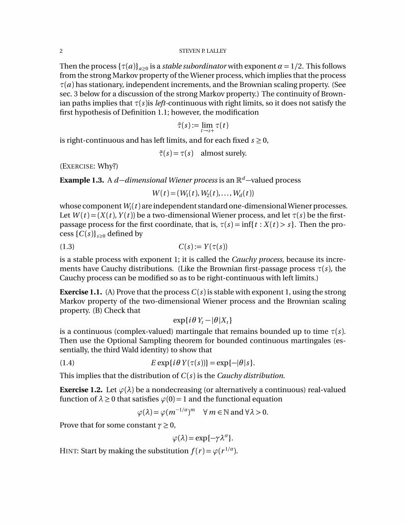
5.6. Stable Processes and Power Laws. The representation of stable subordinatorsand symmetric stable processes by Poisson point processes as given in Corollary 5.4and Exercise 5.1 has some important implications about jump data for such processes.Suppose, for instance, that you were able to record the size of successive jumps in astable-↵ subordinator. Of course, the representation of Corollary 5.4 implies that thereare infinitely many jumps in any finite time interval; however, all but finitely many areof size less than (say) 1. So consider only the data on jumps of size at least 1. Whatwould such data look like?

The Poisson point process representation implies that the number M (y , t ) of jumpsof size at least y occurring before time t is Poisson with mean

t G (y ) := t

Z 1

y

u�↵�1 d u =C t y �↵.

This is what physicists call a power law, with exponent ↵. If you were to plot logG (y )against log y you would get a straight line with slop �↵. If you have enough data fromthe corresponding Poisson point process, and you make a similar log/log plot of theempirical counts, you will also see this straight line. Following is an example for thestable-1/2 subordinator. I ran 1000 simulations of a simple random walk excursion,that is, each run followed a simple random walk until the first visit to +1. I recordedthe duration L of each excursion. (Note: Roughly half of the excursions had L = 1, forobvious reasons; the longest excursion had L = 2, 925, 725.) I sorted these in increasingorder of L , then, for each recorded L , counted N (L ) =number of excursions of durationat least L (thus, for example, N (1) = 1, 000 and N (3) = 503). Here is a plot of log N (L )versus log L :

18 STEVEN P. LALLEY

2 4 6 8 10 12 14

1

2

3

4

5

6

7

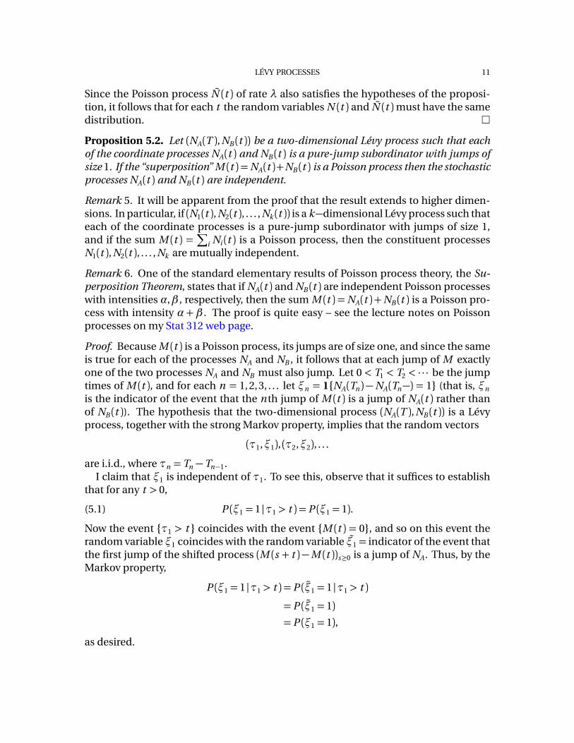
This data clearly follows a line of slope �1/2. Next is a similar simulation for theCauchy process. To (approximately) simulate the jumps of a Cauchy process, start withthe jumps J of a stable-1/2 process, as constructed (approximately) above, and for eachvalue J , run an independent simple random walk for J steps, and record the value S ofthe endpoint. I did this for the 1,000 jump values plotted in the first figure above. Hereis a log/log plot of the resulting |S |�values:

2 4 6 8

1

2

3

4

5

6

7

This data follows a line of slope �1, just as theory predicts. (If you are wonderingwhy there seem to be only half as many points in this plot as in the previous plot, it isbecause I grouped the S� values by their absolute values, and there were only abouthalf as many distinct |S |�values as S�values.)

6. REPRESENTATION THEOREM FOR SUBORDINATORS

Theorem 4. Every subordinator Y (t ) has the form Y (t ) = C t + X (t ), where C � 0 is anonnegative constant and X (t ) is a subordinator of the form (5.7), where N (d t , d y ) is aPoisson point process whose intensity measure µ(d t , d y ) = d t ⌫(d y ) satisfies (5.9).

LÉVY PROCESSES 19

There is a similar – but more complicated – representation for the general Lévy pro-cess, called the Lévy-Khintchine representation. See Kallenberg, for precise statementand complete proof.

The proof of Theorem 4 will be accomplished in two steps. First, we will show that ifY (t ) is a pure jump process then it has the form (5.7) (with X (t ) = Y (t )). Then we willshow that any subordinator is the sum of a pure-jump subordinator and a subordinatorwith continuous paths. Corollary 4.1 will then imply that the continuous part has theform C t for some constant C � 0.

Lemma 6.1. Let Z (t ) be a one-dimensional Lévy process. Then for any Borel set J ⇢ Rthat does not contain a neighborhood of 0 the process

(6.1) NJ (t ) =X

st

1{Z (s )�Z (s�) 2 J }

is a Poisson process. Furthermore, if J1, J2, . . . are non-overlapping intervals then thestochastic processes NJ1

(t ), NJ2(t ), . . . are mutually independent.

Proof. For any t > 0, the sum in (6.1) must be finite, because otherwise the processZ (t ) could not be cadlag. Hence, the process NJ (t ) is well-defined. Since Z (t ) is a Lévyprocess, so is NJ (t ). Clearly, NJ (t ) is a pure jump process whose jumps are all of size 1;therefore, by Proposition 5.1, either NJ (t ) is identically 0 or it is a Poisson process withintensity �J > 0.

If J1, J2, . . . , Jk are non-overlapping intervals then clearly the vector-valued process(NJ1(t ), NJ2

(t ), . . . , NJk(t )) is a Lévy process, because the underlying process Z (t ) has sta-

tionary, independent increments. Moreover, if J =[ik Ji then

NJ (t ) =kX

i=1

NJi(t ).

The process NJ (t ) is itself a Poisson process, so by Proposition 5.2 the processes

NJ1(t ), NJ2

(t ), . . . , NJk(t )

are mutually independent. ⇤

Proof of Theorem 4 for Pure-Jump Subordinators. Assume that Y (t ) is a pure-jump sub-ordinator. By Lemma 6.1, the point process {NB }B⇢(0,1)2 defined by

NB = #jumps (ti , Y (ti )� Y (ti�)) in B

is a Poisson point process. Since Y (t ) is pure-jump, with only positive jumps, for everyt the value Yt must be the sum of the jumps up to time t . Thus,

Y (t ) =ZZ

y 1[0,t ](s )N (d s , d y ).

⇤

20 STEVEN P. LALLEY

Proof of Theorem 4. Let Y (t )be a subordinator. Since Y (t ) is nondecreasing in t , it canhave at most countably many jump discontinuities in any finite time interval [0, t ], andat most finitely many of size � ". Set

YJ (t ) :=X

jumps up to time t ;

then YJ (t ) is a pure-jump subordinator, and therefore has the form (5.7). Moreover, thevector-valued process (Y (t ), YJ (t )) has stationary, independent increments, and henceis a two-dimensional Lévy process. It follows that the process Y (t ) := X (t )� X J (t ) isa subordinator with no jumps. By Corollary 4.1, there is a constant C � 0 such thatY (t ) =C t .

⇤

7. APPENDIX: TOOLS FROM MEASURE THEORY

7.1. Measures and continuous functions. Many distributional identities can be in-terpreted as assertions that two finite measures are equal. For instance, in the identity(3.5), for each fixed set A the right and left sides both (implicitly) define measures onthe Borel subsets B ofRk . The next proposition gives a useful criterion for determiningwhen two finite Borel measures are equal.

Proposition 7.1. Letµ and⌫ be finite Borel measures onRk such that for every bounded,continuous function f :Rk !R,

(7.1)

Zf dµ=Z

f d⌫.

Then µ= ⌫, and (7.1) holds for every bounded Borel measurable function f :Rk !R.

Proof. It suffices to prove that the identity (7.1) holds for every function of the formf = 1B where B 2 Bk , because if it holds for such functions it will then hold for sim-ple functions f , and consequently for all nonnegative functions by monotone conver-gence. Thus, we must show that

(7.2) µ(B ) = ⌫(B ) 8 B 2Bk .

The collection of Borel sets B for which (7.2) holds is a ��system, because both µ and⌫ are countably additive. Hence, it suffices to prove that (7.2) holds for all sets B in a⇡�system that generates the Borel ��algebra. One natural choice is the collectionRof open rectangles with sides parallel to the coordinate axes, that is, sets of the form

R = J1⇥ J2⇥ · · ·⇥ Jk

where each Ji is an open interval in R. To show that (7.2) holds for B = R , I will showthat there are bounded, continuous functions fn such that fn " 1R pointwise; since(7.1) holds for each f = fn , the dominated convergence theorem will then imply that(7.1) holds for f = 1R . To approximate the indicator of a rectangle R from below bycontinuous functions fn , set

fn (x ) =min(1, n ⇥distance(x , R c )).

LÉVY PROCESSES 21

⇤7.2. Poisson Random Measures. To prove that a given collection of random variables{N (B )}B2B is a Poisson point process, one must show that for each B such that µ(B )<1 the random variable N (B ) has a Poisson distribution. Often it is possible to checkthis for sets B of a simple form, e.g., rectangles. The following proposition shows thatthis is enough:

Proposition 7.2. Let {N (B )}B2B be a random measure on (Rk ,Bk )with intensity mea-sure µ. LetR =Rk be the collection of open rectangles with sides parallel to the coordi-nate axes. If

(A) N (B )⇠Poisson-(µ(B )) for each B 2R such that µ(B )<1, and(B) N (Bi ) are mutually independent for all pairwise disjoint sequences Bi 2R ,

then {N (B )}B2B is a Poisson point process.

Proof. First, it is enough to consider only the case where µ(Rk )<1. (Exercise: Checkthis. You should recall that the intensity measure µ was assumed to be ��finite.) Soassume this, and letG be the collection of all Borel sets B for which N (B ) is Poisson withmean µ(B ). This collection is a monotone class2, because pointwise limits of Poissonrandom variables are Poisson. Furthermore, the collection G contains the algebra ofall finite unions of rectangles Ri 2 R , by hypotheses (A)-(B). Hence, by the MonotoneClass Theorem, G =Bk . This proves that N (B ) is Poisson-µ(B ) for every B 2B .

To complete the proof we must show that for every sequence Bi of pairwise disjointBorel sets the random variables N (Bi ) are mutually independent. For this it suffices toshow that for any m � 2 the random variables {N (Bi )}im are independent. I will dothe case m = 2 and leave the general case m � 3 as an exercise.

Denote byA the collection of all finite unions of rectangles R 2R . If A, B 2A aredisjoint, then N (A) and N (B ) are clearly independent, by Hypothesis (B). Let A, B 2Bbe any two disjoint Borel sets: I will show that there exist sequences An , Bn 2 A suchthat

(i) limn!1µ(An�A) = 0;(ii) limn!1µ(Bn�B ) = 0; and

(iii) An \Bn = ; for every n � 1.Since N (An ) and N (Bn ) are independent, for each n , this will imply that N (A) and N (B )are independent. Recall that any Borel set can be arbitrarily well-approximated by fi-nite unions of rectangles, so it is easy to find sequences An and Bn such that (i)-(ii) hold.The tricky bit is to get (iii). But note that if (i) and (ii) hold, then

µ(An \Bn )µ(An�A) +µ(Bn�B )�! 02A collectionM of sets is a monotone class if it is closed under countable increasing unions and

countable decreasing intersections, that is,

(1) If A1 ⇢ A2 ⇢ · · · are elements ofM then so is [n An ; and(2) If B1 � B2 � · · · are elements ofM then so is \n Bn .

22 STEVEN P. LALLEY

Thus, if we replace each Bn by Bn \An then (i)- (iii) will all hold. ⇤Exercise 7.1. Fill in the missing steps of the proof above:

(A) Show that it is enough to consider the case where µ(Rk )<1.(B) Show that if Xn?Yn 8n and Xn ! X a.s. and Yn ! Y a.s., then X?Y .(C) Show how to extend the last part of the argument to m � 3.

UNIVERSITY OF CHICAGO, DEPARTMENT OF STATISTICS, USA