University of Rhode Island Dept. of Electrical and Computer Engineering Kelley Hall 4 East Alumni Ave. Kingston, RI 02881-0805, USA Technical Report No. 082002-1000

Levo - A Scalable Billion Transistor CPU With High IPC

Augustus K. Uht*, David Morano**, Alireza Khalafi** and David Kaeli** *University of Rhode Island and **Northeastern University

Abstract The Levo high ILP microarchitecture is described and evaluated. Levo employs instruction

time-tags and active stations to ensure correct operation in a rampantly speculative and out-of-order resource flow execution model. The Tomasulo-algorithm-like broadcast buses are segmented; their lengths are constant, that is, do not increase with machine size. This helps to make Levo scalable. Known High-ILP techniques such as Disjoint Eager Execution and Minimal Control Dependencies are implemented in novel ways. Examples of basic Levo operation are given. A chip floorplan of Levo is presented, demonstrating feasibility and little cycle-time impact. Levo is simulated, characterizing its basic geometry and its performance.

1 Introduction Levo is a General-Purpose (GP) processor exhibiting large IPC (Instructions Per Cycle) with realistic hardware constraints, scalability and little increase in cycle time. The Levo core exhibits IPC’s greater than 10 on such complex SPECInt benchmarks as gcc and go. The basic Levo operation model is resource flow execution: instructions execute as soon as their operands (speculative or otherwise) are acquired and a Processing Element (PE) is free.

While Levo does use many transistors, billion transistor chips are becoming a reality; further, the trend has always been to use hardware less efficiently as chip transistor densities increased, vis-à-vis all common digital systems. Power and energy consumption are also issues, but we believe it is first necessary to establish the basic performance potential of the microarchitecture; that is the focus of this paper.

In this paper we describe Levo and its operation. We provide detailed simulation results characterizing Levo over a large range of its possible geometries, and present evidence of Levo’s even larger potential performance.

This work was supported in part by the U.S. National Science Foundation under Grants Nos. MIP-9708183 and EIA-9729839, the University of Rhode Island Office of the Provost, the Xilinx Corp., and the Mentor Graphics Corp. David Kaeli is supported by the Ministry of Education, Culture and Sports of Spain. Patents applied for.

1 of 20

The paper is organized as follows. In Section 2 we review major impediments to high IPC realization. Section 3 provides the Levo logical description, and discusses Levo’s solutions to the high IPC problems. Other issues are addressed in Section 4. Section 5 describes the physical operation of Levo and presents a possible Levo single chip floorplan. Section 6 gives our experimental methodology, while Section 7 presents and discusses our simulation results. We conclude in Section 8.

2 High IPC Problems There are three major impediments to high IPC: 1) high and/or unscalable hardware cost; 2) degradation of (increase in) cycle time, negating IPC performance gains; and 3) lack of high-IPC extraction methods. Prior work has shown that there is much ILP (Instruction Level Parallelism) in typical GP code [7]. Large instruction windows and reorder buffers are necessary to realize a fraction of this ILP [13]; these structures greatly exacerbate the first two high-IPC impediments. A system is scalable if its cost grows linearly or less with an increase in the number of Processing Elements or other key elements.1

2.1 High Cost Typical microarchitectures, such as the Pentium P6 [11] and the Alpha EV8 [12], use a large Reorder Buffer to maintain the logical correctness of the code executing out-of-order (OOO). The cost of reorder buffers and other dependency checking/maintaining types of structures [15] is large and does not scale with the number of entries; the typical cost is O(k2) where k is the number of entries in the reorder buffer and/or instruction window, since elements of each entry must be compared to elements of every other entry.

Large pipeline depths also have issues: for a dynamically scheduled high-performance pipeline O(p2) forwarding paths are necessary to reduce or eliminate the ill performance effects of data dependencies between data in different stages, where p is the number of pipeline stages.

2.2 Unscalable Microarchitecture As chip feature sizes shrink, buses become electrically long (high RC time). This leads to longer cycle times and hence reduced overall performance, as does the unscalable hardware mentioned in Section 2.1. Centralized resources such as architectural register files exacerbate the problem. They result in long bus delays and a prohibitively high number of register ports [12]. The latter can increase the size of the register file substantially, further slowing the system.

2.3 Low IPC The high ILP promised over the years has not translated into high IPC or overall performance in a realistic processor, even in machines that did well, such as [8]. Part of the problem is that high-yield ILP methods and combinations of methods have not been attempted with realistic hardware.

1 As many researchers have observed over the years, no system is truly scalable by this definition: as the system

grows, eventually some element grows visibly faster than O(k), often at O(k*log(k)). Within some large values of k, Levo is effectively scalable by our original definition, that is, the multiplier constant for the k*log(k) term is much less than that for the k term; the k term dominates. In traditional systems, the k2 term(s) dominate.

2 of 20

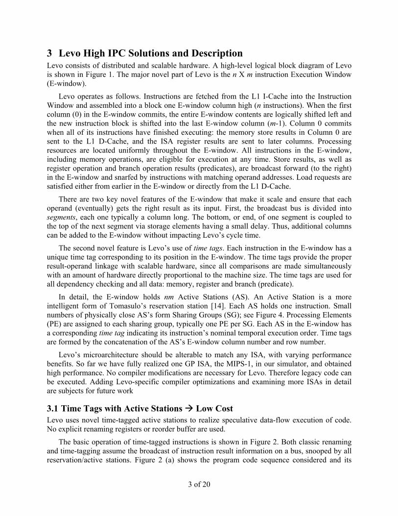
3 Levo High IPC Solutions and Description Levo consists of distributed and scalable hardware. A high-level logical block diagram of Levo is shown in Figure 1. The major novel part of Levo is the n X m instruction Execution Window (E-window).

Levo operates as follows. Instructions are fetched from the L1 I-Cache into the Instruction Window and assembled into a block one E-window column high (n instructions). When the first column (0) in the E-window commits, the entire E-window contents are logically shifted left and the new instruction block is shifted into the last E-window column (m-1). Column 0 commits when all of its instructions have finished executing: the memory store results in Column 0 are sent to the L1 D-Cache, and the ISA register results are sent to later columns. Processing resources are located uniformly throughout the E-window. All instructions in the E-window, including memory operations, are eligible for execution at any time. Store results, as well as register operation and branch operation results (predicates), are broadcast forward (to the right) in the E-window and snarfed by instructions with matching operand addresses. Load requests are satisfied either from earlier in the E-window or directly from the L1 D-Cache.

There are two key novel features of the E-window that make it scale and ensure that each operand (eventually) gets the right result as its input. First, the broadcast bus is divided into segments, each one typically a column long. The bottom, or end, of one segment is coupled to the top of the next segment via storage elements having a small delay. Thus, additional columns can be added to the E-window without impacting Levo’s cycle time.

The second novel feature is Levo’s use of time tags. Each instruction in the E-window has a unique time tag corresponding to its position in the E-window. The time tags provide the proper result-operand linkage with scalable hardware, since all comparisons are made simultaneously with an amount of hardware directly proportional to the machine size. The time tags are used for all dependency checking and all data: memory, register and branch (predicate).

In detail, the E-window holds nm Active Stations (AS). An Active Station is a more intelligent form of Tomasulo’s reservation station [14]. Each AS holds one instruction. Small numbers of physically close AS’s form Sharing Groups (SG); see Figure 4. Processing Elements (PE) are assigned to each sharing group, typically one PE per SG. Each AS in the E-window has a corresponding time tag indicating its instruction’s nominal temporal execution order. Time tags are formed by the concatenation of the AS’s E-window column number and row number.

Levo’s microarchitecture should be alterable to match any ISA, with varying performance benefits. So far we have fully realized one GP ISA, the MIPS-1, in our simulator, and obtained high performance. No compiler modifications are necessary for Levo. Therefore legacy code can be executed. Adding Levo-specific compiler optimizations and examining more ISAs in detail are subjects for future work

3.1 Time Tags with Active Stations Low Cost Levo uses novel time-tagged active stations to realize speculative data-flow execution of code. No explicit renaming registers or reorder buffer are used.

The basic operation of time-tagged instructions is shown in Figure 2. Both classic renaming and time-tagging assume the broadcast of instruction result information on a bus, snooped by all reservation/active stations. Figure 2 (a) shows the program code sequence considered and its

3 of 20

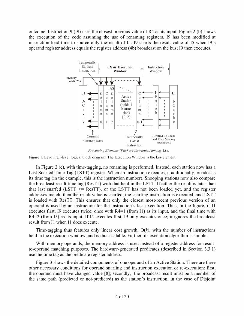
outcome. Instruction 9 (I9) uses the closest previous value of R4 as its input. Figure 2 (b) shows the execution of the code assuming the use of renaming registers. I9 has been modified at instruction load time to source only the result of I5. I9 snarfs the result value of I5 when I9’s operand register address equals the register address (4b) broadcast on the bus; I9 then executes.

Column

0

Column

1

Column

2

Column

m-1

L1

D-Cache

L1

I-Cache

Commit- memory stores

TemporallyEarliest

Instruction

TemporallyLatest

Instruction

AS

ActiveStation(holds 1Instruc-

tion)[0, 2]

n X m ExecutionWindow

I-Fetch

InstructionWindow

(Unified L2 Cacheand Main Memory

not shown.)

Processing Elements (PEs) are distributed among AS’s.

memoryloads

Figure 1. Levo high-level logical block diagram. The Execution Window is the key element.

In Figure 2 (c), with time-tagging, no renaming is performed. Instead, each station now has a Last Snarfed Time Tag (LSTT) register. When an instruction executes, it additionally broadcasts its time tag (in the example, this is the instruction number). Snooping stations now also compare the broadcast result time tag (ResTT) with that held in the LSTT. If either the result is later than that last snarfed (LSTT <= ResTT), or the LSTT has not been loaded yet, and the register addresses match, then the result value is snarfed, the snarfing instruction is executed, and LSTT is loaded with ResTT. This ensures that only the closest most-recent previous version of an operand is used by an instruction for the instruction’s last execution. Thus, in the figure, if I1 executes first, I9 executes twice: once with R4=1 (from I1) as its input, and the final time with R4=2 (from I5) as its input. If I5 executes first, I9 only executes once; it ignores the broadcast result from I1 when I1 does execute.

Time-tagging thus features only linear cost growth, O(k), with the number of instructions held in the execution window, and is thus scalable. Further, its execution algorithm is simple.

With memory operands, the memory address is used instead of a register address for result-to-operand matching purposes. The hardware-generated predicates (described in Section 3.3.1) use the time tag as the predicate register address.

Figure 3 shows the detailed components of one operand of an Active Station. There are three other necessary conditions for operand snarfing and instruction execution or re-execution: first, the operand must have changed value [8]; secondly, the broadcast result must be a member of the same path (predicted or not-predicted) as the station’s instruction, in the case of Disjoint

4 of 20

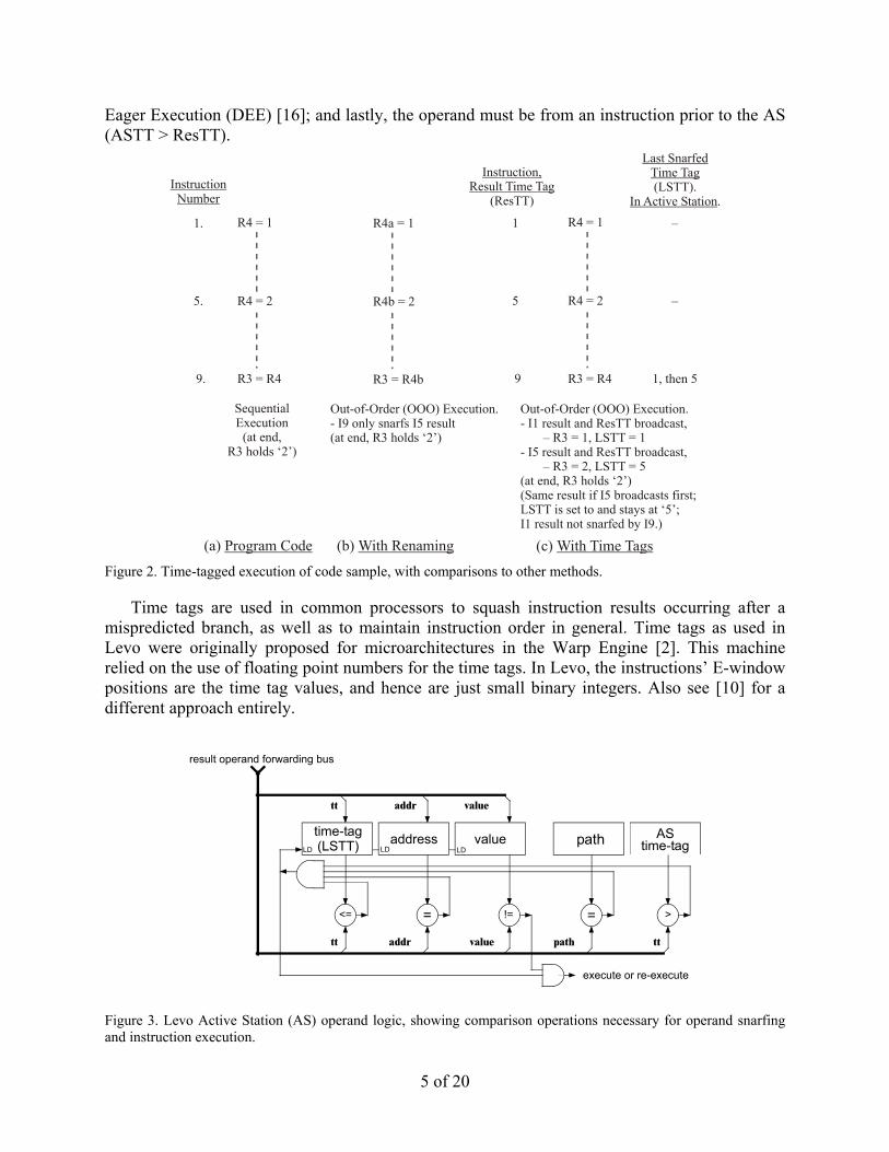
Eager Execution (DEE) [16]; and lastly, the operand must be from an instruction prior to the AS (ASTT > ResTT).

(a) Program Code (b) With Renaming (c) With Time Tags

InstructionNumber

Instruction,Result Time Tag

(ResTT)

1.

5.

9.

1

5

9

R4a = 1

R4b = 2

R3 = R4b

Out-of-Order (OOO) Execution.- I9 only snarfs I5 result(at end, R3 holds ‘2’)

R4 = 1

R4 = 2

R3 = R4

SequentialExecution

(at end,R3 holds ‘2’)

R4 = 1

R4 = 2

R3 = R4

Out-of-Order (OOO) Execution.- I1 result and ResTT broadcast, – R3 = 1, LSTT = 1- I5 result and ResTT broadcast, – R3 = 2, LSTT = 5(at end, R3 holds ‘2’)(Same result if I5 broadcasts first; LSTT is set to and stays at ‘5’;I1 result not snarfed by I9.)

Last SnarfedTime Tag

In Active Station(LSTT).

.

–

–

1, then 5

Figure 2. Time-tagged execution of code sample, with comparisons to other methods.

Time tags are used in common processors to squash instruction results occurring after a mispredicted branch, as well as to maintain instruction order in general. Time tags as used in Levo were originally proposed for microarchitectures in the Warp Engine [2]. This machine relied on the use of floating point numbers for the time tags. In Levo, the instructions’ E-window positions are the time tag values, and hence are just small binary integers. Also see [10] for a different approach entirely.

LDpathtime-tag

(LSTT) value AStime-tag

=

address

=<= >!=

LD LD

execute or re-execute

tt addr value path tt

tt addr value

result operand forwarding bus

Figure 3. Levo Active Station (AS) operand logic, showing comparison operations necessary for operand snarfing and instruction execution.

5 of 20

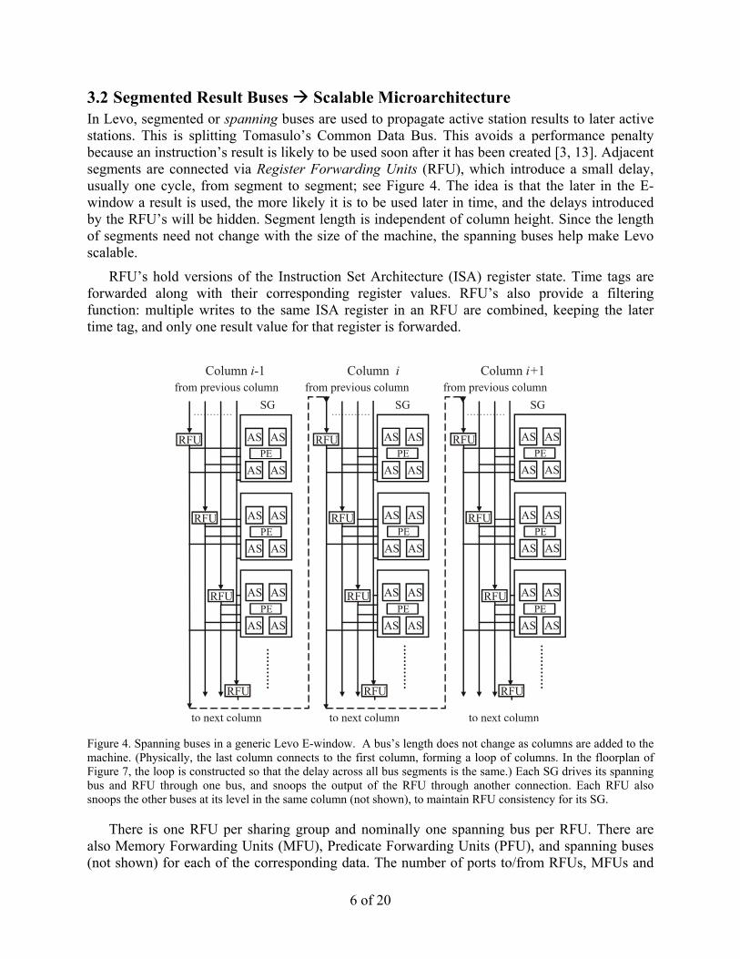
3.2 Segmented Result Buses Scalable Microarchitecture In Levo, segmented or spanning buses are used to propagate active station results to later active stations. This is splitting Tomasulo’s Common Data Bus. This avoids a performance penalty because an instruction’s result is likely to be used soon after it has been created [3, 13]. Adjacent segments are connected via Register Forwarding Units (RFU), which introduce a small delay, usually one cycle, from segment to segment; see Figure 4. The idea is that the later in the E-window a result is used, the more likely it is to be used later in time, and the delays introduced by the RFU’s will be hidden. Segment length is independent of column height. Since the length of segments need not change with the size of the machine, the spanning buses help make Levo scalable.

RFU’s hold versions of the Instruction Set Architecture (ISA) register state. Time tags are forwarded along with their corresponding register values. RFU’s also provide a filtering function: multiple writes to the same ISA register in an RFU are combined, keeping the later time tag, and only one result value for that register is forwarded.

from previous columnfrom previous columnfrom previous column

to next columnto next columnto next column

RFU

AS AS

AS ASPE

RFU

AS AS

AS ASPE

RFU

RFU

AS AS

AS ASPE

RFU

RFU

AS AS

AS AS

PERFU

RFU

AS AS

AS ASPE

RFU

AS AS

AS ASPE

RFU

AS AS

AS ASPE

RFU

AS AS

AS ASPE

RFU

AS AS

AS ASPE

Column 1i- Column 1i+Column i

SGSG SG

Figure 4. Spanning buses in a generic Levo E-window. A bus’s length does not change as columns are added to the machine. (Physically, the last column connects to the first column, forming a loop of columns. In the floorplan of Figure 7, the loop is constructed so that the delay across all bus segments is the same.) Each SG drives its spanning bus and RFU through one bus, and snoops the output of the RFU through another connection. Each RFU also snoops the other buses at its level in the same column (not shown), to maintain RFU consistency for its SG.

There is one RFU per sharing group and nominally one spanning bus per RFU. There are also Memory Forwarding Units (MFU), Predicate Forwarding Units (PFU), and spanning buses (not shown) for each of the corresponding data. The number of ports to/from RFUs, MFUs and

6 of 20

PFUs are small and are constant with respect to the size of the machine; this also helps ensure scalability.

Other novel features are the elimination of a centralized register file, and the simplification of state commitment, both by using RFUs. To see this, assume in the figure that column i-1 is column 0, where instructions are committed. By the time an RFU’s state reaches column 0, it contains the equivalent of what would normally be thought of as the ISA register state. Since the register values have already been broadcast to RFUs in later columns, and since a new column’s (m-1) RFU’s are initialized with the contents of the prior column’s RFU’s, there is always at least one RFU in the E-window that holds the equivalent of the ISA state, no matter the time difference between writing and reading an architectural register; therefore it is unnecessary to save the ISA register state in a separate register file. The same is true of the predicate state. The memory values, however, must be written to the L1 D-cache, since an MFU cannot hold all possible memory locations.

Sometimes instructions must request operands from earlier in the E-window. This is done via backwarding buses (not shown), following the same paths as the forwarding buses, just going in the opposite direction.

3.3 ILP Enhancement Methods High IPC

3.3.1 Hardware Predication Full hardware-based predication is a new implementation of Minimal Control Dependencies. With MCD, all branches may execute concurrently, and the instructions after a branch’s domain [15] may execute independently of the branch. Former hardware-based methods required O(k2) hardware to realize MCD, k being the number of instructions in the E-window, since the control dependency relations of every instruction in the window need to be stored and/or determined with every other instruction in the window. In Levo the cost is O(k), since the amount of predicate storage and computation logic in each AS is constant with respect to the size of the E-window.

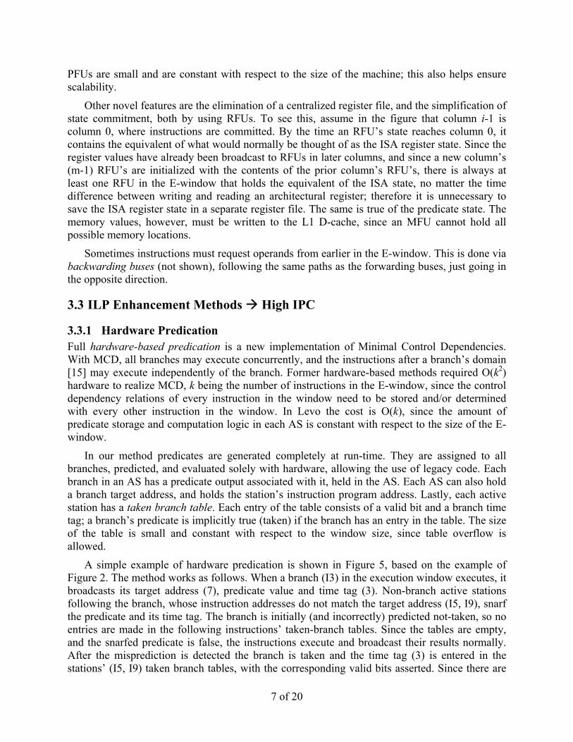
In our method predicates are generated completely at run-time. They are assigned to all branches, predicted, and evaluated solely with hardware, allowing the use of legacy code. Each branch in an AS has a predicate output associated with it, held in the AS. Each AS can also hold a branch target address, and holds the station’s instruction program address. Lastly, each active station has a taken branch table. Each entry of the table consists of a valid bit and a branch time tag; a branch’s predicate is implicitly true (taken) if the branch has an entry in the table. The size of the table is small and constant with respect to the window size, since table overflow is allowed.

A simple example of hardware predication is shown in Figure 5, based on the example of Figure 2. The method works as follows. When a branch (I3) in the execution window executes, it broadcasts its target address (7), predicate value and time tag (3). Non-branch active stations following the branch, whose instruction addresses do not match the target address (I5, I9), snarf the predicate and its time tag. The branch is initially (and incorrectly) predicted not-taken, so no entries are made in the following instructions’ taken-branch tables. Since the tables are empty, and the snarfed predicate is false, the instructions execute and broadcast their results normally. After the misprediction is detected the branch is taken and the time tag (3) is entered in the stations’ (I5, I9) taken branch tables, with the corresponding valid bits asserted. Since there are

7 of 20

one or more entries in each table, the snarfing instructions (I5, I9) are disabled and effectively branched around.

If there is a match between the broadcast target address (7) and a following station’s instruction address (I7), then the instruction is just after the end of the branch’s domain [15] (I4-I6) and should thus be unaffected by the branch’s execution. This station still snarfs the predicate (taken) and its time tag (3) and then rebroadcasts them with the predicate changed to a canceling predicate. Later stations (I9) with a predicate address in their taken branch table matching the canceling predicate address (3) invalidate the table entry (3 to ‘none’); thus, the corresponding branch (I3) no longer affects the operation of the stations (I7-I9), the desired effect.

Once the misprediction is detected and the branch resolves, the now-disabled instructions within the domain that have already executed and broadcast their results must nullify these results and cause dependent instructions to re-execute. In order to do this, the executed-now-disabled instruction (I5) broadcasts a nullify transaction, containing the instruction’s time tag (5) and the register address (R4). Any later instruction (I9) with a matching operand register address (R4) and LSTT equal to the broadcast time tag (5) (dependent instruction) sets itself to the unexecuted state, invalidates its LSTT, and sends a backwards request for the nullified operand (R4). A prior instruction with a valid result (I1), or an RFU, satisfies the request, and execution (of I9 et al) resumes normally.

(a) Program Code (b) With Renamingand NO MCD

(c) With Time Tagsand Hardware Predication

InstructionNumber

Instruction, Predicate,Result Time Tag

(ResTT)

1.

5.

9.

1

5

9

R4a = 1

R4b = 2

R3 = R4(b,a)

Out-of-Order (OOO) Execution.- I3 predicted not taken, so I5 loaded into window,I9 R4 operand renamed to R4b;- I9 snarfs I5 result;- I3 mispredicted,window after I3 is flushed, operand of I9 is changed to R4a;- I9 snarfs I1;(at end, R3 holds ‘1’)

R4 = 1

R4 = 2

R3 = R4

SequentialExecution

(at end,R3 holds ‘1’)

R4 = 1

R4 = 2

R3 = R4

Out-of-Order (OOO) Execution.- I5 result and ResTT broadcast, – R3 = 2;- I3 pred. and ResTT broadcast;- I1 result and ResTT broadcast, – R3 still 2;- branch resolves ‘taken’, I3 pred and ResTT broadcast, I5 and I9 T-B Table entries to 3,

- I5 sends nullify transaction,I9 LSTT matches nullify time tag,I9 sends backwarding request for R4,I5 disabled, so I1 satisfies request, I9 snarfs it;- (at end, R3 holds ‘1’)

I7 matches broadcast branch target address, I7 sends canceling predicate, I9 T-B Table entry cleared, hence I9 enabled;

Taken-Branch TableEntries

In Active Station.

–

none, 3

none, 3, none

3.

7.

IF bc GOTO 7. IF bc GOTO 7. 3

7

IF bc GOTO 7.

– In cases (b) and (c), bc is predicted ‘not taken’, but is mispredicted.

none

Figure 5. Example of Hardware Predication. Compared to both sequential execution and traditional superscalar (non-MCD) execution.

8 of 20

There are other nuances to the correct operation of hardware predication, including overflow of the taken-branch table, an unlikely occurrence. Space precludes their description here; please see [9] for more information.

The cost of hardware predication is low, since most of the extra state storage only takes a few bits in the AS. More buses are needed, but not many more than already exist, and most are only 1 to 8 bits wide. This hardware stays the same for all AS’s and columns with respect to machine size; thus, hardware predication is scalable.

A compiler-assisted form of run-time predication appears in [6]. Only simple hammocks are considered.

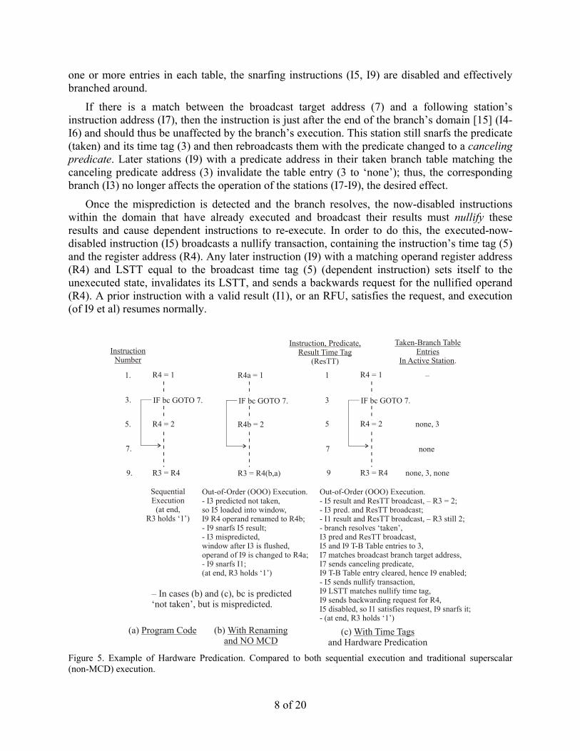
3.3.2 Disjoint Eager Execution (DEE) Both MCD and Disjoint Eager Execution (DEE) are needed for very high ILP [16]. DEE requires the most likely instructions to be executed be given priority for execution resources. In Levo likelihoods are not expressly calculated; instead the “static tree” heuristic of [16] is used. Therefore this is a form of multipath execution in which there is the predicted or mainline path (M) as well as several much shorter not-predicted or disjoint paths (D) spawning from the mainline path at some conditional branches.

DEE is realized in Levo by including AS’s solely dedicated to D-path execution in the Sharing Groups; see Figure 6. Typically, Levo has as many D-path AS’s as M-path AS’s. In effect this means that each Levo E-window column is actually composed of two columns, one for part of the M-path and one for (part of) a D-path. The two columns share the execution, bus and other resources. Mainline AS’s always have priority for the resources. The cost impact of realizing DEE is relatively low: less than 10% greater cost (see Section 5) for a large performance improvement, typically 45%.

D-paths and M-paths execute concurrently, greatly reducing branch misprediction penalties. Conditional branches are assigned to a free D-path (the path is spawned) after they enter the E-window. While DEE operation is somewhat detailed, the example given in Figure 6, based on that in Figure 5 illustrates the basic concepts. It takes one cycle to switch paths, and this is overlapped with instructions’ execution.

Note that D-paths need not occupy the same E-window column as their corresponding M-path column. D-paths can also be multi-column. A D-path can be in any E-window column(s). M-path columns are usually, but not always, in order from left-to-right, holding adjacent code sections in adjacently numbered M-path columns.

4 Other Issues and Levo Solutions

4.1 Instruction Window and I-Fetch The I-Fetch unit fetches whole column(s) of instructions from the I-cache and loads them into the E-window once column(s) there commit. The key here is that instructions are normally fetched in the static or memory order, keeping branches not taken for loading purposes, unless the branch is predicted taken and has a large domain (greater than two-thirds the size of the E-window, in instructions). In that case the fetch becomes dynamic, resuming from the branch target. Initial predicate values for new column(s) are predicted concurrently. This all realizes

9 of 20

simple I-Fetch and high I-fetch bandwidth. It also helps keep branch domains with their branches, so that MCD and DEE can be fully exploited.

Backwards branches are unrolled [15, 16] in the I-Fetch unit, with all but the last instance of the backwards branch converted to a forwards branch to enable/disable loop iterations appropriately. The overall loop body is wrapped around the E-window and continues to execute as long as the last instance of the backwards branch commits taken. When it commits not taken, the loop exits. The unrolling gives good utilization of the E-window for small loops and improves performance.

M-path

Column

0

D-path

3

Column

0

E-WindowColumn 0

PE

AS

ASAS

AS

AS AS

SG M-path

Column

1

D-path

5

Column

0

E-WindowColumn 1

PE

AS AS

AS AS

SG M-path

Column

m-1

D-path

2

Column

0

E-WindowColumn m-1

PE

AS AS

AS AS

SG1. R4 =1 1. R4 =1

3. IF bc GOTO 7.(bc is false; branch

is not taken)

3. IF bc GOTO 7.(bc set true; branchis taken)

5. R4 =2 5. R4 =2

7. 7.

9. R3 = R4 9. R3 = R42 1 Figure 6. Sample arrangement and DEE operation of Mainline (M) path columns and DEE (D) path columns. The code example is from Figure 5. D-path spawning: D-path 5 is available and is spawned from the branch (I3) in M-path 0 by broadside loading it with the same instructions as in M-path 0, from an I-Fetch buffer (not re-fetched from memory); the D-path branch is set to the opposite state of the spawned branch in M-path 0. Then both paths execute: respective I9’s hold different values of R3. After the spawned branch resolves (it was mispredicted), D-path 5 becomes M-path 0: I9 now has the correct result for R3 (1); the old D-path 5 results are rebroadcast to other M-paths (1 to m-1); the old M-path 0 state is thrown out.

Subroutine calls are conditionally inlined in hardware by the I-Fetch unit: when a call is encountered fetching is retargeted to the start of the subroutine, if the call is not in the domain of a predicted-taken branch. Subroutine returns are unconditionally inlined: when a return is encountered, fetching is retargeted to the return address. Return stack(s) are used to aid the process.

4.2 Large Memory Latencies – Modified Memory System The deep E-window in Levo provides a large tolerance to main memory latency, up to 800 cycles or more [5] with assumptions similar to those in Section 6. Similar observations have been

10 of 20

made by Karkhanis and Smith [4]. These latencies are typical of what is expected in the next few years.

Store data is buffered in the E-window. Each MFU is chained to the next column’s MFU, as with the RFUs. However, an MFU’s internal structure is different. There is an L0 cache and a Previous Column Buffer (PCB). The PCB has n entries and holds the accumulated stores from the previous column, holding only the latest value for a given memory store address. PCB’s are used to distribute the store buffering throughout the machine and reduce the amount of buffered information. Once committed, and thus in column 0, one PCB’s worth of stores (from column 0) are sent to the L1 D-cache to update the memory state.

Load requests are handled with memory backwarding buses. Loads can be satisfied from either earlier active stations, earlier MFUs, the L1 D-cache or higher up in the hierarchy. The result is forwarded as a store.

As will be seen in Section 5, the physical realization of the Levo memory system employs multiple copies of the L1 D-cache to keep the access time to the cache low (1 cycle) and to keep cache access bandwidth high. The cache copies hold the same data, within a few cycles, with all of them replacing the same lines at the same time. While the loads from the different cache copies are likely to be different, the stores are always the same to all of the copies.

5 Physical Considerations: Column Renaming and Chip Floorplan Levo avoids physically shifting the E-window by renaming the columns. Each physical column has one or more registers associated with it that hold its logical column number. When a logical left shift occurs, the logical column numbers of all of the columns are decremented. Recall that time tags throughout the machine are formed from the concatenation of the logical column number and the fixed row number of the corresponding active station; therefore, as left shifts occur the time tags are automatically corrected and their values re-used. Therefore the column renaming greatly simplifies the machine wiring, and eliminates the power consumption associated with a physical shift.

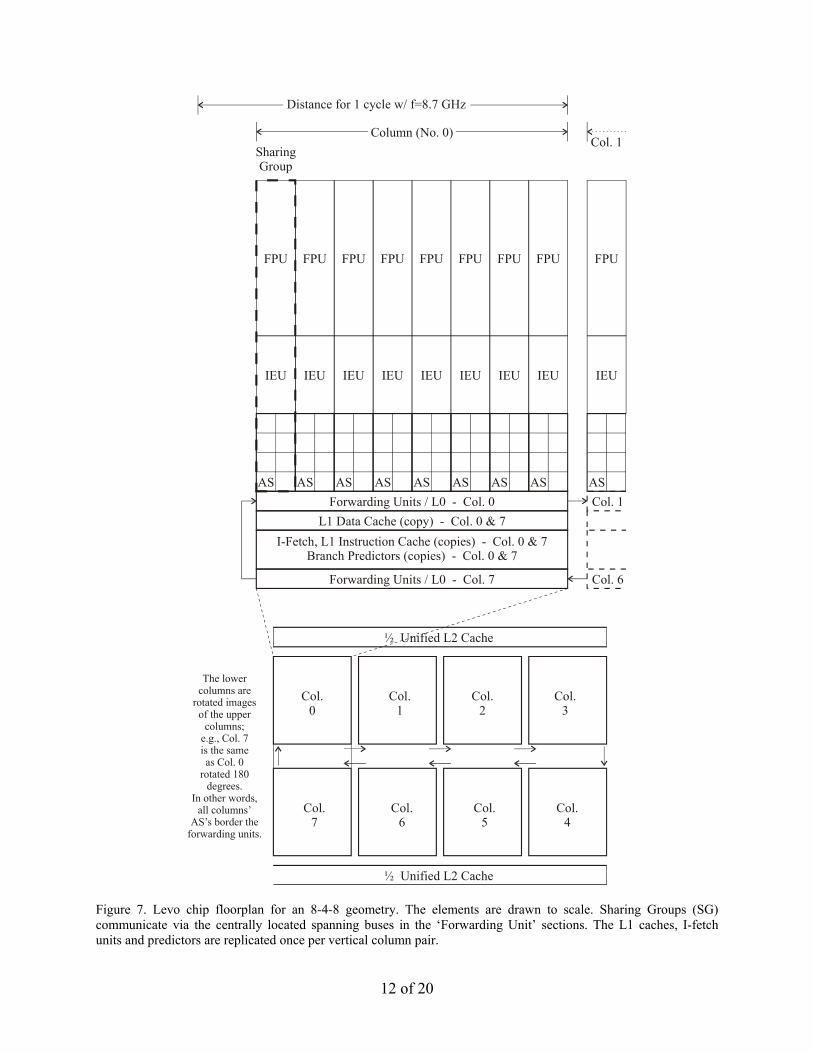
A Levo chip floorplan is shown in Figure 7. The goal was to demonstrate Levo realizability on a single chip within the next few years; the goal was not area optimization or exactness per se. The Compaq/Intel EV8 chip floorplan and dimensions [12] were used to size similar Levo structures, as well as to ensure that the critical path is not substantially increased by the Levo microarchitecture.

The geometry used is 8-4-8, that is, 8 sharing groups per column, 4 M-path and 4 D-path active stations per sharing group, 8 M-path columns and 8 D-path columns (8 E-window columns, total). One FPU (Floating Point Unit) and one IEU (Integer Execution Unit) form the PE of each sharing group. 64-bit data paths and machine architecture are also assumed.

In the floorplan the columns’ spanning buses are physically oriented end-to-end and in a loop to keep the critical path length low. Every active station within a column is accessible from every other active station in the same column within one clock cycle. The delay from one forwarding unit to the next is one cycle or less. Assuming a target clock frequency of 10 GHz, possible within a few years, the realized clock frequency should be about 87% of this, that is, a performance loss of about 13%. This is offset much more by the IPC speedup of Levo for the geometry considered, at least a factor of 2.

11 of 20

AS

IEU

FPU

SharingGroup

AS

IEU

FPU

AS

IEU

FPU

AS

IEU

FPU

AS

IEU

FPU

AS

IEU

FPU

AS

IEU

FPU

AS

IEU

FPU

AS

IEU

FPU

Column (No. 0)

Distance for 1 cycle w/ f=8.7 GHz

Col. 1

Forwarding Units / L0 - Col. 0

Forwarding Units / L0 - Col. 7

L1 Data Cache (copy) - Col. 0 & 7I-Fetch, L1 Instruction Cache (copies) - Col. 0 & 7

Branch Predictors (copies) - Col. 0 & 7

Col. 1

Col. 6

Col.0

Col.1

Col.2

Col.3

Col.7

Col.6

Col.5

Col.4

½ Unified L2 Cache

½ Unified L2 Cache

The lowercolumns are

rotated imagesof the upper

columns;e.g., Col. 7is the sameas Col. 0

rotated 180degrees.

In other words,all columns’

AS’s border theforwarding units.

Figure 7. Levo chip floorplan for an 8-4-8 geometry. The elements are drawn to scale. Sharing Groups (SG) communicate via the centrally located spanning buses in the ‘Forwarding Unit’ sections. The L1 caches, I-fetch units and predictors are replicated once per vertical column pair.

12 of 20

The Levo chip as described above is estimated to use about 600 million transistors; this is derived from both actual VHDL synthesis of key components [17] as well as rough estimates from the EV8 work. The current cost of the branch predictors is included in the above estimates, but the predictors are not included in the floorplan since they have not been tuned. The data value predictors are not included in either the cost or the floorplan since they currently add little to the performance, and thus are not needed. Note that Levo’s cost could be vastly reduced with fewer FPU’s (not needed for much GP code) or a 32-bit data path.

Also note that Levo is easily scalable. For example, in order to increase the machine size only pairs of columns need to be added to either end of the center channel and inserted in the physical loop; the cycle time is unaffected.

6 Experimental Methodology A cycle-accurate trace-based simulator (FastLevo) was written to model Levo’s key structures and measure its performance. FastLevo uses traces of MIPS-1 machine code (32-bit machine). The latter is generated from the benchmarks with a native SGI compiler using the ‘-O’ optimization and ‘-o32’ MIPS-1 switch. (FastLevo also simulates the few MIPS-2 instructions occurring in the relevant SGI compiler libraries.)

Ten SPECInt benchmarks were simulated: SPECInt95: compress, go, ijpeg SPECInt2000: bzip2, crafty, gcc, gzip, mcf, parser, vortex

Each benchmark was simulated for 100 million instructions with data gathering turned off, to warm up the predictors and caches and ignore program initialization. Data was gathered during the simulation of the next 500 million instructions. The benchmarks’ reference inputs were used, except for compress, for which the buffer size was reduced so that compress completed its initialization section within the first 100 million instructions.

The common machine assumptions are shown in Table 1.

Table 1. Levo default parameter values.

Parameter Value

Branch predictor 2-level gshare w/ 1024 BHT and 4096 GPHT, 2-bit saturating counter, one per E-window row.

Data value predictor computational-stride predictor w/ 4096 entries, 2 source operands per entry, 2-bit saturating counter per operand, one per E-window row.

Word size 32 bits

Processing Element latencies/pipelining Same as MIPS R4000.

L0 hit latency 1 cycle

L0 size 32 one-word entries

L0 configuration Fully-associative

L0 block size 1 word

L1-I,D hit latency 1 cycle (cache access time itself; does not include 1 cycle bus delay)

13 of 20

L1-I,D size (each) 64 KBytes

L1-I,D configuration 2-way set associative

L1-I,D block size 32 bytes

L2 (unified I/D) hit latency 10 cycles

L2 size 2 MBytes

L2 configuration Direct-mapped

L2 block size 32 bytes

Main memory latency (no misses) 100 cycles

Main memory interleave factor 4

Return stacks 2, 16 entries each. (in I-Fetch unit)

Spanning bus delay (no contention)

1 cycle

Forwarding Unit delay (no bus contention)

1 cycle

Buses per RFU and per MFU 2 input and 2 output buses

Buses per PFU 1 input and 1 output bus

M-path to D-path column switch Switch itself: 1 cycle. D-path results broadcast as bus resources permit.

Columns per D-path 1 column

7 Experimental Evaluation and Characterization The major sets of experiments were: microarchitecture assumptions verification, performance sensitivity to machine geometry, and performance effect of ideal/real I-Fetch and memory systems. For a point of comparison, the SimpleScalar/PISA [1] machine model (similar to MIPS-1) gave an IPC of 1.96, assuming an unrealizable 32-way issue conventionally-constructed superscalar machine, with the same benchmark assumptions.

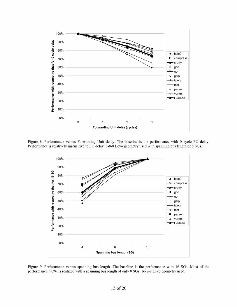
7.1 Microarchitecture Assumptions’ Verification We first hypothesized that buses can be segmented with non-zero delay forwarding units inserted between the segments. Figure 8 presents the performance degradation experienced when the forwarding unit delay is increased from 0 to 3 cycles. It is seen that the typical delay, 1 cycle, is easily tolerated, having a performance loss of 6%, confirming the hypothesis.

We also hypothesized that buses need only be some fixed length (as a machine design increases) to capture most of the performance. Figure 9 shows the performance improvement with increasing bus length, conservatively assuming a constant spanning bus delay of 1 cycle. It is seen that there is only an 11% performance increase when doubling the spanning bus length from 8 to 16 SGs, with a much larger improvement of 29% going from 4 SGs to 8 SGs; therefore, a spanning bus length of 8 is necessary and adequate, and the hypothesis is confirmed.

7.2 Levo Geometry Effects on Performance In this set of experiments each machine geometry dimension was varied with the other two dimensions held constant. See Figure 10 for the results.

14 of 20

0%

10%

20%

30%

40%

50%

60%

70%

80%

90%

100%

0 1 2 3Forwarding Unit delay (cycles)

Perf

orm

ance

with

resp

ect t

o th

at fo

r 0 c

ycle

del

aybzip2compresscraftygccgogzipijpegmcfparservortexH-mean

Figure 8. Performance versus Forwarding Unit delay. The baseline is the performance with 0 cycle FU delay. Performance is relatively insensitive to FU delay. 8-8-8 Levo geometry used with spanning bus length of 8 SGs.

0%

10%

20%

30%

40%

50%

60%

70%

80%

90%

100%

4 8 16Spanning bus length (SG)

Perf

orm

ance

with

resp

ect t

o th

at fo

r 16

SG

bzip2compresscraftygccgogzipijpegmcfparservortexH-Mean

Figure 9. Performance versus spanning bus length. The baseline is the performance with 16 SGs. Most of the performance, 90%, is realized with a spanning bus length of only 8 SGs. 16-8-8 Levo geometry used.

15 of 20

bzip2

0.0%

10.0%

20.0%

30.0%

40.0%

50.0%

60.0%

4 8 12 16

Geometry element (x)

Impr

ovem

ent o

ver b

asel

ine

compress

0.0%

10.0%

20.0%

30.0%

40.0%

50.0%

60.0%

70.0%

4 8 12 16

Geometry element (x)

Impr

ovem

ent o

ver b

asel

ine

crafty

0.0%

10.0%

20.0%

30.0%

40.0%

50.0%

60.0%

4 8 12 16

Geometry element (x)

Impr

ovem

ent o

ver b

asel

ine

gcc

0.0%

5.0%

10.0%

15.0%

20.0%

25.0%

30.0%

35.0%

40.0%

45.0%

50.0%

4 8 12 16Geometry element (x)

Impr

ovem

ent o

ver b

asel

ine

go

0.0%

10.0%

20.0%

30.0%

40.0%

50.0%

60.0%

4 8 12 16Geometry element (x)

Impr

ovem

ent o

ver b

asel

ine

gzip

0.0%

10.0%

20.0%

30.0%

40.0%

50.0%

60.0%

70.0%

80.0%

90.0%

4 8 12 16Geometry element (x)

Impr

ovem

ent o

ver b

asel

ine

ijpeg

0.0%

20.0%

40.0%

60.0%

80.0%

100.0%

120.0%

140.0%

160.0%

4 8 12 16Geometry element (x)

Impr

ovem

ent o

ver b

asel

ine

mcf

0.0%

10.0%

20.0%

30.0%

40.0%

50.0%

60.0%

4 8 12 16Geometry element (x)

Impr

ovem

ent o

ver b

asel

ine

parser

0.0%

5.0%

10.0%

15.0%

20.0%

25.0%

30.0%

35.0%

40.0%

45.0%

4 8 12 16Geometry element (x)

Impr

ovem

ent o

ver b

asel

ine

vortex

0.0%

10.0%

20.0%

30.0%

40.0%

50.0%

60.0%

70.0%

80.0%

4 8 12 16Geometry element (x)

Impr

ovem

ent o

ver b

asel

ine

Harmonic Mean

0.0%

10.0%

20.0%

30.0%

40.0%

50.0%

60.0%

4 8 12 16Geometry element (x)

Impr

ovem

ent o

ver b

asel

ine

SG/Col: x-4-8

AS/SG: 8-x-8

Cols: 8-4-x

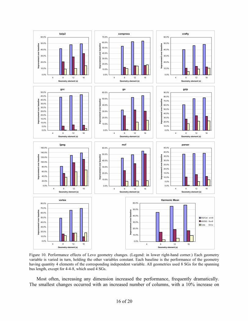
Figure 10. Performance effects of Levo geometry changes. (Legend: in lower right-hand corner.) Each geometry variable is varied in turn, holding the other variables constant. Each baseline is the performance of the geometry having quantity 4 elements of the corresponding independent variable. All geometries used 8 SGs for the spanning bus length, except for 4-4-8, which used 4 SGs.

Most often, increasing any dimension increased the performance, frequently dramatically. The smallest changes occurred with an increased number of columns, with a 10% increase on

16 of 20

average when going from 4 to 16 columns. The largest changes were seen with increased Sharing Groups per column, with a 55% increase in performance going from 4 to 12 SG/col. While increasing columns and SG/col gave monotonically increasing trends, increasing the AS/SG gave varying trends. This is to be expected: the former changes increase the number of PE’s, while the latter only determines PE utilization, which varies across benchmarks due to code variations. On average, there was no need to go above 12 AS/SG, which gave a 19% improvement over 4 AS/SG. Part of the reason(s) why the gain in performance for increased SG/col is greater than that for an increased number of columns, but only part of the reason, is the short spanning bus length (4) of the baseline (4-4-8) for SG/col; see Figure 9.

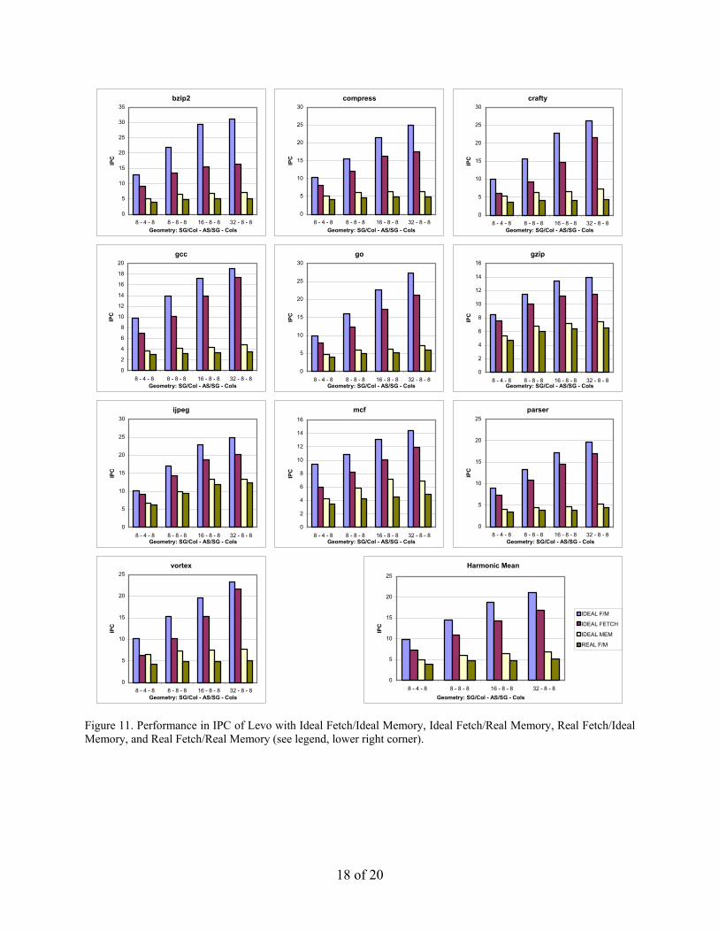
7.3 Ideal/Real IPC Performance The effects of ideal/real I-Fetch and an ideal/real memory system were examined for several different machine geometries. Ideal I-Fetch is realized by using oracles for the branch predictors at instruction load time. An ideal memory system is realized by assuming 100% L1 data and instruction cache hit rates. The results are presented in Figure 11; all four combinations of ideal/real – I-Fetch/memory system are shown, each for four machine geometries. IPC ranges from a low of about 4 to a high of about 31. We have also seen IPC’s of up to 80 with a 64-16-16 geometry and 4 buses per forwarding unit (not shown in the figure).

Overall, we have three major conclusions from these results. First, with realistic assumptions and a current-sized geometry (8-4-8), we are not yet able to realize high IPC (the harmonic mean is about 4 IPC). Second, good news, there is still more IPC to get, given the high ideal numbers (about 10 IPC for the 8-4-8 geometry). Lastly, the memory system functions well with or without Ideal I-Fetch, primarily leaving the I-Fetch system to be improved. One possible solution is to simply use a single much better branch predictor for the static/dynamic I-Fetch decision itself. We are also pursuing much more advanced solutions, including trace caches and also using DEE in the I-Fetch unit.

7.4 Other Levo Characteristics’ Results Five other additional experiments were performed, again over all benchmarks, to investigate certain other performance characteristics of Levo. The experiments, their results and conclusions are presented in Table 2. A Levo 8-4-8 geometry was used throughout.

8 Summary One billion transistor microarchitectures have many daunting requirements: high IPC, high main memory latency tolerance, high clock rates, and ability to execute legacy codes. Further, such machines must honor hard chip realization constraints such as scalable structures and short buses. This paper has proposed the Levo microarchitecture, targeted to satisfy all of these requirements. The reorder buffer and scalable bussing structure issues have been thoroughly addressed and resolved in Levo. The performance simulation results are very encouraging, both verifying the basic tenets of the resource flow model and demonstrating IPC’s in the 10’s for the Levo core E-window and memory system. We are currently pursuing improvements including more accurate I-Fetch and data value prediction.

17 of 20

bzip2

0

5

10

15

20

25

30

35

8 - 4 - 8 8 - 8 - 8 16 - 8 - 8 32 - 8 - 8Geometry: SG/Col - AS/SG - Cols

IPC

compress

0

5

10

15

20

25

30

8 - 4 - 8 8 - 8 - 8 16 - 8 - 8 32 - 8 - 8Geometry: SG/Col - AS/SG - Cols

IPC

crafty

0

5

10

15

20

25

30

8 - 4 - 8 8 - 8 - 8 16 - 8 - 8 32 - 8 - 8Geometry: SG/Col - AS/SG - Cols

IPC

gcc

0

2

4

6

8

10

12

14

16

18

20

8 - 4 - 8 8 - 8 - 8 16 - 8 - 8 32 - 8 - 8Geometry: SG/Col - AS/SG - Cols

IPC

go

0

5

10

15

20

25

30

8 - 4 - 8 8 - 8 - 8 16 - 8 - 8 32 - 8 - 8Geometry: SG/Col - AS/SG - Cols

IPC

gzip

0

2

4

6

8

10

12

14

16

8 - 4 - 8 8 - 8 - 8 16 - 8 - 8 32 - 8 - 8Geometry: SG/Col - AS/SG - Cols

IPC

ijpeg

0

5

10

15

20

25

30

8 - 4 - 8 8 - 8 - 8 16 - 8 - 8 32 - 8 - 8Geometry: SG/Col - AS/SG - Cols

IPC

mcf

0

2

4

6

8

10

12

14

16

8 - 4 - 8 8 - 8 - 8 16 - 8 - 8 32 - 8 - 8Geometry: SG/Col - AS/SG - Cols

IPC

parser

0

5

10

15

20

25

8 - 4 - 8 8 - 8 - 8 16 - 8 - 8 32 - 8 - 8Geometry: SG/Col - AS/SG - Cols

IPC

vortex

0

5

10

15

20

25

8 - 4 - 8 8 - 8 - 8 16 - 8 - 8 32 - 8 - 8Geometry: SG/Col - AS/SG - Cols

IPC

Harmonic Mean

0

5

10

15

20

25

8 - 4 - 8 8 - 8 - 8 16 - 8 - 8 32 - 8 - 8Geometry: SG/Col - AS/SG - Cols

IPC

IDEAL F/M

IDEAL FETCH

IDEAL MEM

REAL F/M

Figure 11. Performance in IPC of Levo with Ideal Fetch/Ideal Memory, Ideal Fetch/Real Memory, Real Fetch/Ideal Memory, and Real Fetch/Real Memory (see legend, lower right corner).

18 of 20

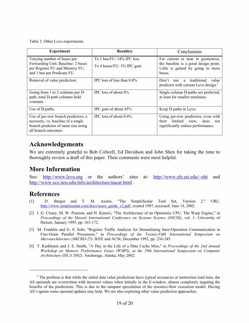
Table 2. Other Levo experiments.

Experiment Result(s) Conclusions Varying number of buses per Forwarding Unit. Baseline: 2 buses per Register FU and Memory FU, and 1 bus per Predicate FU.

To 1 bus/FU: 14% IPC loss

To 4 buses/FU: 3% IPC gain

For current or near in geometries, the baseline is a good design point. Little is gained by going to more buses.

Removal of value prediction. IPC loss of less than 0.8% Don’t use a traditional value predictor with current Levo design.2

Going from 1 to 2 columns per D-path, total D-path columns held constant.

IPC loss of about 8% Single column D-paths are preferred, at least for smaller machines.

Use of D-paths. IPC gain of about 45% Keep D-paths in Levo.

Use of per-row branch predictors, a necessity, vs. baseline of a single branch predictor of same size using all branch outcomes.

IPC loss of about 0.4% Using per-row predictors, even with their limited view, does not significantly reduce performance.

Acknowledgements We are extremely grateful to Bob Colwell, Ed Davidson and John Shen for taking the time to thoroughly review a draft of this paper. Their comments were most helpful.

More Information See: http://www.levo.org or the authors’ sites at: http://www.ele.uri.edu/~uht and http://www.ece.neu.edu/info/architecture/nucar.html .

References [1] D. Burger and T. M. Austin, "The SimpleScalar Tool Set, Version 2," URL:

http://www.simplescalar.com/docs/users_guide_v2.pdf, created 1997, accessed: June 14, 2002.

[2] J. G. Cleary, M. W. Pearson, and H. Kinawi, "The Architecture of an Optimistic CPU: The Warp Engine," in Proceedings of the Hawaii International Conference on Systems Science (HICSS), vol. 1: University of Hawaii, January 1995, pp. 163-172.

[3] M. Franklin and G. S. Sohi, "Register Traffic Analysis for Streamlining Inter-Operation Communication in Fine-Grain Parallel Processors," in Proceedings of the Twenty-Fifth International Symposium on Microarchitecture (MICRO-25): IEEE and ACM, December 1992, pp. 236-245.

[4] T. Karkhanis and J. E. Smith, "A Day in the Life of a Data Cache Miss," in Proceedings of the 2nd Annual Workshop on Memory Performance Issues (WMPI), at the 29th International Symposium on Computer Architecture (ISCA 2002). Anchorage, Alaska, May 2002.

2 The problem is that while the initial data value predictions have typical accuracies at instruction load time, the

AS operands are overwritten with incorrect values when initially in the E-window, almost completely negating the benefits of the predictions. This is due to the rampant speculation of the resource-flow execution model. Having AS’s ignore some operand updates may help. We are also exploring other value prediction approaches.

19 of 20

20 of 20

[5] A. Khalafi, D. A. Morano, D. R. Kaeli, and A. K. Uht, "Realizing High IPC Through a Scalable Memory-Latency Tolerant Multipath Microarchitecture," Department of Electrical and Computer Engineering, University of Rhode Island, Kingston, RI 02881-0805, Technical Report 032002-0101, April 2, 2002.

[6] A. Klauser, T. Austin, D. Grunwald, and B. Calder, "Dynamic Hammock Predication for Non-predicated Instruction Set Architectures," in Intl. Conf. on Parallel Architectures and Compilation Techniques (PACT). Paris, France, October 1998, pp. 278-285.

[7] M. S. Lam and R. P. Wilson, "Limits of Control Flow on Parallelism," in Proceedings of the 19th Annual International Symposium on Computer Architecture. Gold Coast, Australia: IEEE and ACM, May 1992, pp. 46-57.

[8] M. H. Lipasti and J. P. Shen, "Superspeculative Microarchitecture for Beyond AD 2000," IEEE COMPUTER, vol. 30, no. 9, pp. 59-66, September 1997.

[9] D. Morano, "Execution-Time Instruction Predication," Dept. of Electrical and Computer Engineering, University of Rhode Island, Kingston, RI 02881, Technical Report 032002-0100, March 2002.

[10] R. Nagarajan, K. Sankaralingam, D. Burger, and S. Keckler, "A Design Space Evaluation of Grid Processor Architectures," in Proceedings of the 30th Annual ACM/IEEE International Symposium on Microarchitecture. Austin, Texas USA: ACM, December 2001.

[11] D. B. Papworth, "Tuning the Pentium Pro Microarchitecture," IEEE MICRO, vol. 16, no. 2, pp. 8-15, April 1996.

[12] R. P. Preston, R. W. Badeau, D. W. Bailey, S. L. Bell, L. L. Biro, W. J. Bowhill, D. E. Dever, S. Felix, R. Gammack, V. Germini, M. K. Gowan, P. Gronowski, D. B. Jackson, S. Mehta, S. V. Morton, J. D. Pickholtz, M. H. Reilly, and M. J. Smith, "Design of an 8-wide Superscalar RISC Microprocessor with Simultaneous Multithreading," in Proceedings of the International Solid State Circuits Conference, January 2002. Slides from talk at conference also referenced.

[13] G. S. Sohi, S. Breach, and T. N. Vijaykumar, "Multiscalar Processors," in Proceedings of the 22nd Annual International Symposium on Computer Architecture: IEEE and ACM, June 1995.

[14] R. M. Tomasulo, "An Efficient Algorithm for Exploiting Multiple Arithmetic Units," IBM Journal of Research and Development, vol. 11, no. 1, pp. 25-33, January 1967.

[15] A. K. Uht, "A Theory of Reduced and Minimal Procedural Dependencies," IEEE Transactions on Computers, vol. 40, no. 6, pp. 681-692, June 1991. Also in the tutorial ``Instruction-Level Parallel Processors'', Torng, H.C., and Vassiliadis, S., Eds., IEEE Computer Society Press, 1995, pages 171-182.

[16] A. K. Uht and V. Sindagi, "Disjoint Eager Execution: An Optimal Form of Speculative Execution," in Proceedings of the 28th International Symposium on Microarchitecture (MICRO-28). Ann Arbor, MI, November/December 1995, pp. 313-325. URL: ftp://ele.uri.edu/pub/uht/micro95.ps.

[17] T. Wenisch and A. K. Uht, "HDLevo - VHDL Modeling of Levo Processor Components," Department of Electrical and Computer Engineering, University of Rhode Island, Kingston, RI, Technical Report 072001-100, July 20, 2001.