
Leveraging the Language Modeling Approach to Information
39
Effective Use of Phrases in Language Modeling to Improve Information Retrieval Maojin Jiang, Eric Jensen, Steve Beitzel Information Retrieval Laboratory Illinois Institute of Technology {jianmao, ej, steve}@ir.iit.edu Shlomo Argamon Linguistic Cognition Group Illinois Institute of Technology [email protected] Abstract Traditional information retrieval models treat the query as a bag of words, assuming that the occurrence of each query term is independent of the positions and occurrences of others. Several of these traditional models have been extended to incorporate positional information, most often through the inclusion of phrases. This has shown improvements in effectiveness on large, modern test collections. The language modeling approach to information retrieval is attractive because it provides a well-studied theoretical framework that has been successful in other fields. Incorporating positional information into language models is intuitive and has shown significant improvements in several language-modeling applications. However, attempts to integrate positional information into the language-modeling approach to IR have not shown consistent significant improvements. This paper provides a broader exploration of this problem. We apply the backoff technique to incorporate a bigram phrase language model with the traditional unigram one and compare its performance to an interpolation of a conditional bigram model with the unigram model. While this novel application of backoff does not improve effectiveness, we find that our formula for interpolating a conditional bigram model with the unigram model yields significantly different results from prior work. Namely, it shows an 11% relative improvement in average precision on one query set, while yielding no improvement on the other two. 1. Introduction Information retrieval traditionally views queries and documents as a bag of words Salton75 , implying that the occurrence of each term is independent from occurrences of all other terms. This is obviously inaccurate and it is easy to find examples of its failures. Financial documents, for example, would likely have many instances of the word “exchange” following the word “stock,” whereas agricultural documents may talk more about the “exchange of livestock.” Prior attempts at integrating phrases into other information retrieval models have shown improvements in retrieval effectiveness on modern test collections.
Transcript of Leveraging the Language Modeling Approach to Information
Effective Use of Phrases in Language Modeling to Improve Information Retrieval
Maojin Jiang, Eric Jensen, Steve Beitzel
Information Retrieval Laboratory Illinois Institute of Technology {jianmao, ej, steve}@ir.iit.edu
Shlomo Argamon
Linguistic Cognition Group Illinois Institute of Technology
Abstract Traditional information retrieval models treat the query as a bag of words, assuming that the occurrence of each query term is independent of the positions and occurrences of others. Several of these traditional models have been extended to incorporate positional information, most often through the inclusion of phrases. This has shown improvements in effectiveness on large, modern test collections. The language modeling approach to information retrieval is attractive because it provides a well-studied theoretical framework that has been successful in other fields. Incorporating positional information into language models is intuitive and has shown significant improvements in several language-modeling applications. However, attempts to integrate positional information into the language-modeling approach to IR have not shown consistent significant improvements. This paper provides a broader exploration of this problem. We apply the backoff technique to incorporate a bigram phrase language model with the traditional unigram one and compare its performance to an interpolation of a conditional bigram model with the unigram model. While this novel application of backoff does not improve effectiveness, we find that our formula for interpolating a conditional bigram model with the unigram model yields significantly different results from prior work. Namely, it shows an 11% relative improvement in average precision on one query set, while yielding no improvement on the other two.
1. Introduction Information retrieval traditionally views queries and documents as a bag of words Salton75, implying that the occurrence of each term is independent from occurrences of all other terms. This is obviously inaccurate and it is easy to find examples of its failures. Financial documents, for example, would likely have many instances of the word “exchange” following the word “stock,” whereas agricultural documents may talk more about the “exchange of livestock.” Prior attempts at integrating phrases into other information retrieval models have shown improvements in retrieval effectiveness on modern test collections.
The language modeling approach to information retrieval ranks documents’ similarity to queries by modeling them as statistical language models and calculating the probability of one given the other Ponte98. However, the traditional term independence assumption is typically applied. Attempts to incorporate phrases into language models have not shown consistent, significant improvements on modern test collections. These techniques have all been based on slightly different linear interpolations of unigram word probabilities with bigram phrase probabilities. We propose the backoff strategy, which has been successful in using language models for speech recognition Katz87, as an attempt to garner the improvements seen from phrases in other retrieval strategies.
2. Prior Work Prior work in this area consists of on the development of the language modeling approach to information retrieval, the incorporation of phrases into that methodology through interpolation, and the incorporation of phrases into other retrieval strategies.
2.1. Language Modeling in Information Retrieval The language modeling approach to information retrieval ranks documents based on
)( qdp , the probability that a document generates an observed query. Since this is difficult to measure directly, however, Bayes Theorem is often applied and a document-independent constant is dropped (Equation 1).
)()()( ...1...1 dpdqqpqqdp nn ∝
Equation 1: Language Model Document Ranking
In practice , the prior probability that a document is relevant to any query, is assumed to be uniform. Also common in most work is that the next step: applying the bag of words assumption (Equation 2) by estimating the probability of the sequence as the product of the probabilities of the individual terms.
)(dp
∏≈
iin dqpdqqp )()( ...1
Equation 2: Unigram Language Model
Since a document is a very sparse language model, the next necessary step is for this estimate to be smoothed to account for query terms unseen in the document. This is typically accomplished by incorporating the probability of the unseen term in the collection as a whole through one of the many smoothing methods available (such as the successful Dirichlet smoothing in Equation 3). Katz’ backoff technique has also been compared to smoothing for the case of unseen terms and did not perform as effectively Zhai01.
1
1 )();()(
µµ
µ +⋅+
=d
CqpdqCdqp iMLEi
i
);( dqC i is the frequency of query term in document iq dd is the number of terms in document d
)( Cqp iMLE is the maximum likelihood estimate of the probability of q in the collection i
Equation 3: Dirichlet Smoothed Unigram Model
2.2. Incorporating Phrases There has been much work attempting to use phrases to enhance the effectiveness of information retrieval. Most often this does not show more than a 10% improvement over the simple bag of words approach, with improvements closer to 5% being more common Mitra97 Kraaij98 Turpin99 Narita00 Chowdhu01a. However, phrases consistently provide some improvement in retrieval strategies outside the language modeling paradigm, rarely harming retrieval performance. Several methodologies for integrating phrases have been tried inside the language modeling framework. Although they are all based on a linear interpolation of bigram and unigram models, they differ slightly in formulation and significantly in their results, albeit on differing collections. Song and Croft used a linear interpolation of unigram and joint bigram probabilities1 inside the document in combination with a linear interpolation for smoothing unseen unigrams by )( Cqp i , the probability of a term in the corpus as a whole (Equation 4) Song99.
)()1()()( Cqpdqpdqp iii ⋅−+⋅≈ ϖω
)()1(),(),( 11 dqpdqqpdqqp iiiii ⋅−+⋅≈ −− λλ
Equation 4: Song and Croft Bigram Interpolation
In their experimentation, they empirically set 40.=ϖ and 90.=λ and saw a relative improvement in average precision over their smoothed unigram language model of 7% for the TREC 4 queries on the Wall Street Journal collection and less than 1% on the entire TREC 4 collection. Miller, Leek, and Schwartz used a single three-way linear interpolation of unigram and conditional bigram document probabilities and unigram collection probabilities (Equation 5) Miller99.
∏ −⋅+⋅+⋅≈i
iiiin dqqpadqpaCqpadqqp )),()()(()( 1210...1
Equation 5: Miller, Leek, and Schwartz Bigram Interpolation
1 The use of the joint probability here is unclear, as we would not expect the unigram probability to be a reasonable estimate for the bigram joint probability.
They empirically set , 70.0 =a 29.1 =a , and 01.2 =a and saw less than 5% relative improvement in average precision over their smoothed unigram language model on the TREC 6 and 7 queries over the 2GB SGML collection from TREC disks 4 & 5. Hiemstra describes a similar strategy for integrating proximity into his hidden Markov model framework Hiemstra01. All of these approaches treat phrases as lower-weighted units while counting the terms making up the phrases at a higher weight. This is often explained heuristically by citing the high weights associated with phrases due to their rarity in the collection (their collection probabilities are much smaller than their document probabilities) and the corresponding need to normalize for this. Work outside of the language modeling framework shows that phrase weighting based simply on query lengths can be as effective as static weights empirically tuned and tested on the same 50 TREC queries Chowdhu01a. Interactive work with users manually selecting phrases from the lexicon to expand their queries has suggested that the addition of certain phrases can significantly improve average precision Smeaton98. The authors suggest that since phrases have very different frequency distributions than individual terms, integrating phrases with the unigram words used in queries may require two separate term-weighting functions and thus a more fusion-centered approach similar to what has been used to combine other forms of multiple query representations Chowdhu01b.
3. Methodology We further explore the problem of integrating phrases into language models for information retrieval by applying the backoff technique that has been successful in other applications. As our baseline, we propose an alternative interpolation of conditional bigram and unigram models that seeks to maintain a separation between the bigram interpolation parameter and the unigram smoothing parameter (Equation 6).
)()1(),(),( 11 dqpdqqpdqqp iiiii ⋅−+⋅≈ −− λλ
Equation 6: Conditional Bigram Interpolation
Note that this technique counts unigram influence in combination with bigram influence for its final estimation. Our backoff strategy uses unigram term probabilities only when those terms do not form a phrase that appears in the document (Equation 7).
),(),( 11 dqqpdqqp iidmlii −− ≈ if dqq ii ∈− ,1
)()( 1 dqpdqp iid ⋅⋅ −α otherwise
Equation 7: Backoff from Bigrams to Unigrams
In fact, the amount of the overall probability space dedicated to unigram probabilities is explicitly defined by the document-dependent constant given in Equation 8, which is determined by ),( 1 dqqp iidml − , the discounted maximum likelihood estimate specific to the discounting method used Zhai01. In this work, we use the Dirichlet discounting method given by Equation 9.
∑
∑
∉
∈
⋅
−=
Dww
Dwwdml
d DwpDwp
Dwwp
21
21
)|()|(
)|(1
21
21
α
Equation 8: Probability space reserved for unseen bigrams in each document
2
11 1
);,(),(µ+−
= −− d
dqqCdqqp iiiidml
Equation 9: Dirichlet Discounted Maximum Likelihood Joint Bigram Model
In order to practically use this backoff formulation, we must deal with joint bigram probabilities by converting them to conditional probabilities in order to combine them term-by-term as in Equation 10.
∏= −
−⋅≈n
i i
iin dqp
dqqpdqpdqqp
2 1
11...1 )|(
)()|()(
Equation 10: Converting Joint Bigram Probabilities to Conditionals for Combination
Note that using interpolation parallels previous methods of incorporating phrases (inside and outside of the language modeling framework) by regarding phrase matches as an added boost to their component term matches, whereas backoff stresses phrase matches by excluding influence of their component terms. As such the method of phrase selection used with backoff may have a more significant impact than seen in prior studies Mitra97 Kraaij98. In this work, we simply use all sequentially appearing pairs of terms (statistical phrases), as a basic bigram model would be defined. Linear interpolation should perform well when phrases consist of terms that carry their own meaning, such as “academic journal”, whereas backoff should perform well when phrases consist of terms that should effectively be stopped if they are inside the phrase such as “New York”.
4. Experimentation We use the TREC 6, 7, and 8 short title (1-4 terms) queries’ against the TREC disks 4 and 5 2GB collection of SGML (primarily news) data with our lab’s search engine, AIRE, to examine average precision when including the bigram distribution through each of our methods. The only retrieval utilities we use are a 342-word stop list from Cornell’s SMART search engine, and a hand-built list of conflation classes in favor of a stemmer. For each model, we empirically find a semi-optimal set of smoothing parameters, publishing these tuning experiments to illustrate stability of smoothing and combination parameters across varying models. We first tune our unigram smoothing
parameter for each set of queries. We then incorporate bigram probabilities through linear interpolation as in Equation 6, and also through backoff as in Equation 7.
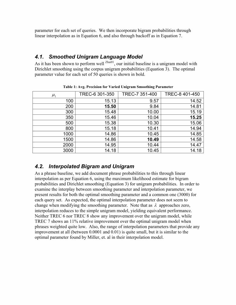
4.1. Smoothed Unigram Language Model As it has been shown to perform well Zhai01, our initial baseline is a unigram model with Dirichlet smoothing using the corpus unigram probabilities (Equation 3). The optimal parameter value for each set of 50 queries is shown in bold.
Table 1: Avg. Precision for Varied Unigram Smoothing Parameter
1µ TREC-6 301-350 TREC-7 351-400 TREC-8 401-450 100 15.13 9.57 14.52200 15.50 9.84 14.81300 15.48 10.00 15.19350 15.46 10.04 15.25500 15.38 10.30 15.06800 15.18 10.41 14.94
1000 14.86 10.45 14.851500 14.86 10.49 14.582000 14.95 10.44 14.473000 14.18 10.45 14.18
4.2. Interpolated Bigram and Unigram As a phrase baseline, we add document phrase probabilities to this through linear interpolation as per Equation 6, using the maximum likelihood estimate for bigram probabilities and Dirichlet smoothing (Equation 3) for unigram probabilities. In order to examine the interplay between smoothing parameter and interpolation parameter, we present results for both the optimal smoothing parameter and a common one (3000) for each query set. As expected, the optimal interpolation parameter does not seem to change when modifying the smoothing parameter. Note that as λ approaches zero, interpolation reduces to the simple unigram model, yielding equivalent performance. Neither TREC 6 nor TREC 8 show any improvement over the unigram model, while TREC 7 shows an 11% relative improvement over the optimal unigram model when phrases weighted quite low. Also, the range of interpolation parameters that provide any improvement at all (between 0.0001 and 0.01) is quite small, but it is similar to the optimal parameter found by Miller, et. al in their interpolation model.

Table 2: Avg. Precision for Varied Bigram Interpolation Parameter
λ TREC-6 301-350
2001 =µ
TREC-6 301-350
30001 =µ
TREC-7 351-400
15001 =µ
TREC-7 351-400
30001 =µ
TREC-8 401-450
3501 =µ
TREC-8 401-450
30001 =µ0.00005 15.5 14.05 10.57 10.51 15.25 15.250.0001 15.5 14.07 10.63 10.53 15.25 15.250.001 15.43 14.24 11.05 11.31 15.25 14.630.005 15.40 14.73 11.66 11.48 15.15 14.790.01 15.38 14.69 11.59 11.32 15.09 14.810.1 15.02 14.14 10.52 10.53 14.16 13.710.4 14.47 13.85 10.11 10.12 13.75 13.440.6 14.36 13.83 10.03 9.95 13.74 13.44
4.3. Backoff from Bigram to Unigram Finally, we examine our backoff strategy. Again, we offer results for both the optimal unigram smoothing parameter and a fixed one. Unfortunately, we see no improvement for any query set. In TREC 7 and TREC 8, performance is impaired by approximately 10%. In terms of the discount parameter, performance is much more stable with a wide range of values than that of interpolation, indicating that we likely did not simply miss the optimal parameter. The large magnitude of the optimal discount parameter, devoting more of the probability space to the unigram model we back off to, may indicate that using phrases without incorporating their component unigram probabilities is unwise. We hypothesize that the reason performance does not approach that of the unigram model even when the parameter is drastically large is due to the additional document length factor that is introduced by the document-dependent backoff constant. As with interpolation, the optimal discount parameter does not seem to change significantly when modifying the smoothing parameter.
Table 3: Avg. Precision for Varied Bigram Backoff Discount Parameter
2µ TREC-6 301-350
2001 =µ
TREC-6 301-350
5001 =µ
TREC-7 351-400
15001 =µ
TREC-7 351-400
5001 =µ
TREC-8 401-450
3501 =µ
TREC-8 401-450
5001 =µ 1000 14.89 14.56 9.16 9.25 12.79 13.393000 14.20 14.65 9.26 9.66 13.68 12.795000 15.05 14.67 9.68 9.69 13.71 13.71
10000 14.77 14.82 9.65 9.37 13.59 13.7850000 14.24 14.02 9.70 9.47 13.79 13.8890000 13.71 13.94 9.61 9.37 13.65 13.90
100000 13.67 13.67 9.56 9.31 13.59 14.00110000 13.62 13.74 9.49 9.26 13.52 13.95150000 13.24 13.23 9.52 9.05 13.20
5. Conclusion and Future Work We have explored using the backoff technique to incorporate phrases into language models for information retrieval. This technique has proved unsuccessful when using all sequentially appearing pairs of terms as phrases. We have also shown that phrases can help significantly when interpolating them as conditional bigram probabilities with the unigram model. Future work will examine intelligently selecting phrases when applying the backoff strategy and performing an in-depth analysis of why phrases help so much on one set of topics but do not show any improvement on others. Salton75 G. Salton, C.S. Yang, and A. Wong,. A Vector-Space Model for Automatic Indexing. In Communications of the ACM 18(11):613-620, 1975. Ponte98 J. Ponte and W. B. Croft. A language modeling approach to information retrieval. In 21st ACM Conference on Research and Development in Information Retrieval (SIGIR’98) 275-281, 1998. Katz87 S. M. Katz. Estimation of probabilities from sparse data for the language model component of a speech recognizer. In IEEE Transactions on Acoustics, Speech, and Signal Processing, 35:400-401, 1987. Zhai01 C. Zhai and J. Lafferty. A study of smoothing methods for language models applied to ad hoc information retrieval. In 24th ACM Conference on Research and Development in Information Retrieval (SIGIR’01) 334-342, 2001. Mitra97 M. Mitra, C. Buckley, A. Singhal, C. Cardie. An Analysis of Statistical and Syntactic Phrases. In 5th International Conference Recherche d'Information Assistee par Ordinateur (RIAO’97), 1997. Kraaij98 W. Kraaij and R. Pohlmann. Comparing the effect of syntactic vs. statistical phrase index strategies for dutch. In C. Nikolaou and C. Stephanidis (Eds.) Proceedings of the 2nd European Conference on Research and Advanced Technology for Digital Libraries (ECDL’98) 605-617. Turpin99 A. Turpin and A. Moffat. Statistical phrases for Vector-Space information retrieval. In 22nd ACM Conference on Research and Development in Information Retrieval (SIGIR’99) 309-310, 1999. Narita00 M. Narita and Y. Ogawa. The use of phrases from query texts in information retrieval. In 23rd ACM Conference on Research and Development in Information Retrieval (SIGIR’00) 318-320, 2000. Chowdhu01a A. Chowdhury. Adaptive Phrase Weighting. In International Symposium on Information Systems and Engineering (ISE 2001), 2001. Song99 F. Song and W. B. Croft. A general language model for information retrieval. In Eighth International Conference on Information and Knowledge Management (CIKM’99), 1999. Miller99 D. R. H. Miller, T. Leek, and R. M. Schwartz. A hidden Markov model information retrieval system. In 22nd ACM Conference on Research and Development in Information Retrieval (SIGIR’99) 214-221, 1999. Hiemstra01 D. Hiemstra. Using language models for information retrieval. Center for Telematics and Information Technoloy, 2001. VIII, 164 p. : ill. ; 25 cm. - (CTIT Ph.D thesis series, ISSN 1381-3617 ; no. 01-32), 2001. Smeaton98 A. F. Smeaton and F. Kelledy. User-chosen phrases in interactive query formulation for information retrieval. In 20th BCS-IRSG Colloquium, Springer-Verlag Electronic Workshops in Computing, 1998. Chowdhu01b A. Chowdhury, S. Beitzel, E. Jensen. Analysis of Combining Multiple Query Representations in a Single Engine. In 2002 IEEE International Conference on Information Technology - Coding and Computing (ITCC), 2002.
Text Categorization for Authorship Verification
Moshe Koppel Jonathan Schler Dror Mughaz
Dept. of Computer Science Bar-Ilan University Ramat-Gan, Israel
Abstract. One common version of the authorship attribution problem is that of authorship verification. We need to determine whether a given author, for whom we have a corpus of writing samples, is also the author of a given anonymous text. The set of alternate candidates is not limited to a given finite closed set. In this paper we show how usual text categorization methods can be adapted to solve the authorship verification problem given a sufficiently large anonymous text. The main trick is a type of robustness test in which the best discriminators between two corpora are iteratively eliminated: if texts remain distinguishable as the discriminators are eliminated, they are very likely by different authors.
1. Authorship verification
The same text categorization methods used for classification text by topic [1] can be
used for authorship attribution [2-4]. Given sufficiently large samples of two or more
authors’ work, we can in principle learn models to distinguish them. Typically, the
feature sets used for such attribution tasks will involve topic-neutral attributes [5-7]
such as function words or parts-of-speech n-grams rather than the content words
usually used for topic classification.
One common version of the authorship attribution problem is that of authorship
verification. We need to determine whether a given author (for whom we have a
corpus of writing samples) is also the author of a given anonymous text. The set of
alternate candidates is not limited to a given finite closed set. Thus, while there is no
shortage of negative examples, we can never be sure that these negative examples
fully represent the space of all alternative authors.
In this paper we show how usual text categorization methods can be adapted to solve
the authorship verification problem given a sufficiently large anonymous text. In
particular, we will show that a judicious combination of applications of standard
classification methods can be used to unmask authors writing pseudonymously or
anonymously even when the authors’ known writings differ chronologically or
thematically from the unattributed texts.
2. A Motivating Example
Let us begin by considering a real-world example. We are given two 19th century
collections of Hebrew-Aramaic responsa (letters written in response to legal queries).
The first, RP (Rav Pe'alim) includes 509 documents authored by an Iraqi rabbinic
scholar known as Ben Ish Chai. The second, TL (Torah Lishmah) includes 524
documents that Ben Ish Chai, claims to have found in an archive. There is ample
historical reason to believe that he in fact authored the manuscript but did not wish to
take credit for it for personal reasons.
We are given four more collections of responsa written by four other authors working
in the same area during the same period. While these far from exhaust the range of
possible authors, they collectively constitute a reasonable starting point. To make it
interesting, we will refer to Ben Ish Chai, the author of RP, as the “suspect”, to the
author of TL as the “mystery man”, and the other four as “impostors”. The object is to
determine if the suspect is “guilty”; is he in fact the mystery man?
2.1 Pairwise authorship attribution
We will combine a number of pairwise authorship attribution experiments in order to
solve the verification problem. Let’s begin by reviewing four stages of pairwise
authorship attribution:
1. Cleanse the texts.
Since the texts we have of the responsa may have undergone some editing, we must
make sure to ignore possible effects of differences in the texts resulting from variant
editing practices. Thus, we eliminate all orthographic variations: we expand all
abbreviations and unify variant spellings of the same word.
2. Select an appropriate feature set.
We select a list of lexical features as follows: the 200 most frequent words in the
corpus are selected and all those that are deemed content-words are eliminated
manually. We are left with 130 features. Strictly speaking, these are not all function
words but rather words that are typical of the legal genre generally, without being
correlated with any particular sub-genre. Thus, in the responsa context, a word like
question would be allowed although in other contexts it would not be considered a
function word.
3. Represent the documents as vectors.
Each individual responsum is represented as a vector of dimension 130, each entry of
which represents the relative frequency (normalized by document length) of a
respective feature.
4. Learn models.
Using each responsum as a labeled example, we use a variant of Exponential Gradient
[8,9] as our learner to distinguish pairs of collections.
2.2 From attribution to verification
We begin by checking whether we are able to distinguish between the suspect’s work,
RP, and that of each of the four impostors, using standard text categorization
techniques. Five-fold cross-validation accuracy results for RP against each impostor
are shown in Table 1. Note that we obtain accuracy of greater than 95% for each case.
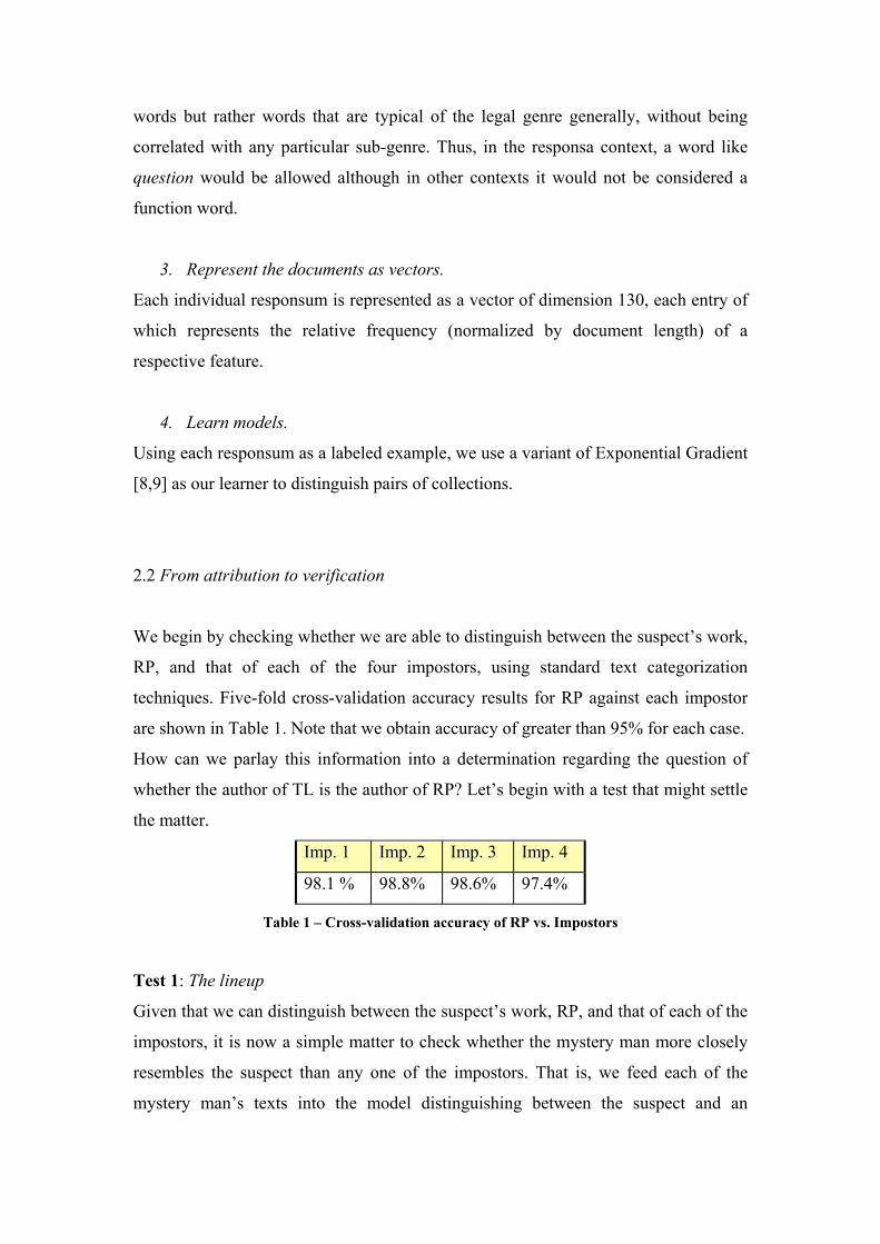
How can we parlay this information into a determination regarding the question of
whether the author of TL is the author of RP? Let’s begin with a test that might settle
the matter.
Imp. 1 Imp. 2 Imp. 3 Imp. 4
98.1 % 98.8% 98.6% 97.4%
Table 1 – Cross-validation accuracy of RP vs. Impostors
Test 1: The lineup
Given that we can distinguish between the suspect’s work, RP, and that of each of the
impostors, it is now a simple matter to check whether the mystery man more closely
resembles the suspect than any one of the impostors. That is, we feed each of the
mystery man’s texts into the model distinguishing between the suspect and an

impostor and check if a significant number of them are more similar to an impostor. If
so, it would be highly unlikely that the suspect actually authored these documents.
In our case, however, this is not what happens. In fact, as shown in Table 2, for each
impostor, the vast majority of mystery man’s documents are classified as more similar
to the suspect than to the impostor. Does this prove that the suspect is in fact our
mystery man? It certainly does not. It simply shows that the suspect is a more likely
candidate to be the mystery man than are these four impostors. But it may very well
be that neither any of the impostors nor the suspect is the mystery man and that the
true author of TL is still at large. Thus, for our case, this test is indecisive.
Imp. 1 Imp. 2 Imp. 3 Imp. 4
95.4 % 92.2% 87.6% 96.2%
Table 2 - Percentage of TL docs classified as RP vs. impostors
Test 2: Composite sketch
The next test is to determine whether the suspect and the mystery man resemble each
other. All we need to do is to see whether there is a model that successfully
distinguishes between documents in RP and documents in TL, using cross-validation
accuracy as a measure. If no such model can be found, this would constitute strong
evidence that the author of RP and of TL are one and the same, particularly if there
are successful models for distinguishing between the mystery man and each of the
impostors. Thus, we begin by learning models to distinguish between the mystery
man’s work, TL, and that of each of the impostors. Cross-validation accuracy results
are shown in Table 3. It turns out that the mystery man and the suspect are, in fact,
easily distinguishable, with cross-validation accuracy of 98.5%. Does this mean that
the author of RP is not the author of TL?
RP Imp. 1 Imp. 2 Imp. 3 Imp. 4
98.5% 99.0 % 99.0% 97.3% 94.9%
Table 3 – Cross-validation accuracy for TL vs. others
A cursory glance at the texts indicates that the results do not necessarily support such
a conclusion. The author of TL simply used certain stock phrases, which do not appear
in RP, in a very consistent manner. The author of RP could easily have written TL and
used such a ruse to deliberately mask his identity. Thus, this test is also indecisive.
Test 2a: Unmasking
Our objective is to determine whether two corpora are distinguishable based on many
differences – probably indicating different authors – or based solely on a few features.
Difference regarding only a few features might not indicate different authors; a small
number of differences are to be expected even in different works by a single author as
a result of varying content, purposes, genres, chronology, or even deliberate
subterfuge by the author.
We wish then to test the depth of difference between TL and RP, as well as – for
comparison—between TL and each of the impostors. We already have effective
models to distinguish TL from each other author. For each such model, we eliminate
the five highest-weighted features in each direction and then learn a new model. We
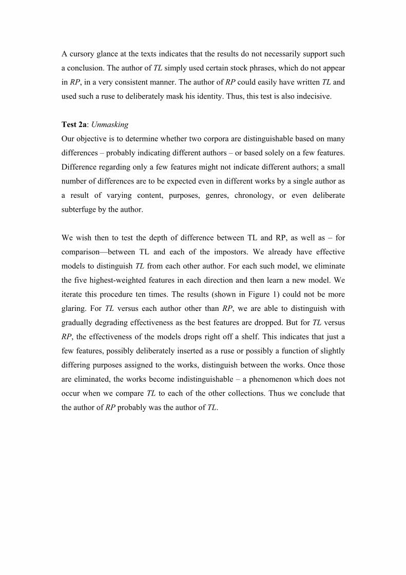
iterate this procedure ten times. The results (shown in Figure 1) could not be more
glaring. For TL versus each author other than RP, we are able to distinguish with
gradually degrading effectiveness as the best features are dropped. But for TL versus
RP, the effectiveness of the models drops right off a shelf. This indicates that just a
few features, possibly deliberately inserted as a ruse or possibly a function of slightly
differing purposes assigned to the works, distinguish between the works. Once those
are eliminated, the works become indistinguishable – a phenomenon which does not
occur when we compare TL to each of the other collections. Thus we conclude that
the author of RP probably was the author of TL.
50
60
70
80
90
100
1 2 3 4 5 6 7 8 9 10 11
Figure 1 – Cross-validation accuracy of TL vs. others as best features are iteratively dropped.
The x-axis represents the number of iterations. The dotted line is TL vs. RP
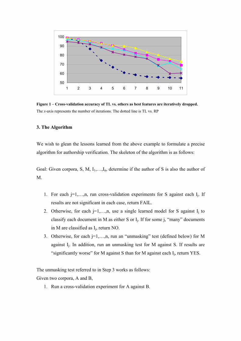
3. The Algorithm
We wish to glean the lessons learned from the above example to formulate a precise
algorithm for authorship verification. The skeleton of the algorithm is as follows:
Goal: Given corpora, S, M, I1,…,In, determine if the author of S is also the author of
M.
1. For each j=1,…,n, run cross-validation experiments for S against each Ij. If
results are not significant in each case, return FAIL.
2. Otherwise, for each j=1,…,n, use a single learned model for S against Ij to
classify each document in M as either S or Ij. If for some j, “many” documents
in M are classified as Ij, return NO.
3. Otherwise, for each j=1,…,n, run an “unmasking” test (defined below) for M
against Ij. In addition, run an unmasking test for M against S. If results are
“significantly worse” for M against S than for M against each Ij, return YES.
The unmasking test referred to in Step 3 works as follows:
Given two corpora, A and B,
1. Run a cross-validation experiment for A against B.
2. Using a single model for A against B, eliminate the k highest-weighted
features. (A linear separator, such as Winnow or linear SVM automatically
provides such weights.)
3. Go to step 1.
Clearly, the terms “many” and “significantly worse” are not well-defined. In the
remainder of this paper, we will run a number of systematic experiments to determine
how to define some of these terms more precisely. We will focus specifically on the
parameters necessary for better specifying the unmasking algorithm.
4. Experiments
For each experiment in this section, we choose works in a single genre (broadly
speaking) by two or three authors who lived in the same country during the same
period. We choose multiple works by at least one of these authors. (See Table 4 for
the full list of works used in each experiment.) For each pair of works we run an
unmasking test using linear SVM [10] as our learner. The object is to find consistent
differences in the curves produced by unmasking tests on two corpora by the same
author and those produced by unmasking tests on two corpora by different authors.
For our purposes, a corpus is simply a book divided into chunks. In these
experiments, each book was divided into at least 50 chunks containing not less than
300 words. The initial feature set consisted of the 100 most frequent words in the
corpus; at each stage of unmasking, we eliminate five features. In Figures 2-5, we
show the results of these unmasking tests. In each, we divide the results between (a)
comparisons of two books by a single author and (b) comparisons of books by two
different authors in the same group. Results are reported in terms of classification
accuracy.
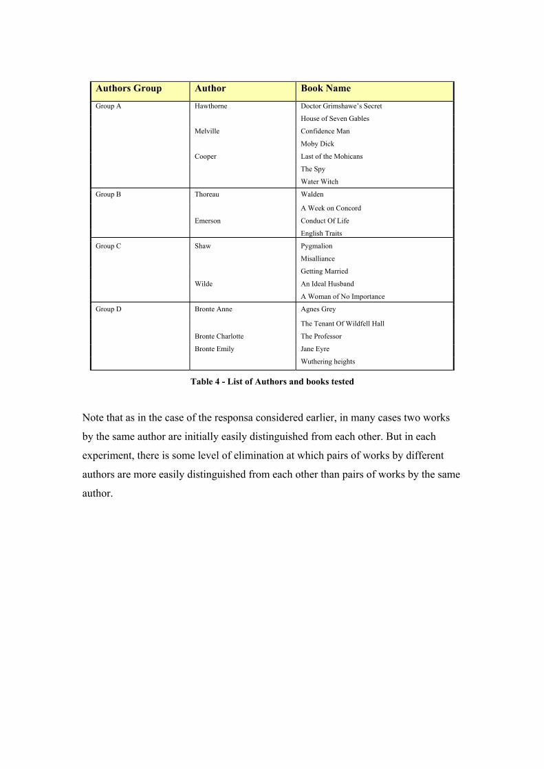
Authors Group Author Book Name
Doctor Grimshawe’s Secret Hawthorne
House of Seven Gables
Confidence Man Melville
Moby Dick
Last of the Mohicans
The Spy
Group A
Cooper
Water Witch
Walden Thoreau
A Week on Concord
Conduct Of Life
Group B
Emerson
English Traits
Pygmalion
Misalliance
Shaw
Getting Married
An Ideal Husband
Group C
Wilde
A Woman of No Importance
Agnes Grey Bronte Anne
The Tenant Of Wildfell Hall
Bronte Charlotte The Professor
Jane Eyre
Group D
Bronte Emily
Wuthering heights
Table 4 - List of Authors and books tested
Note that as in the case of the responsa considered earlier, in many cases two works
by the same author are initially easily distinguished from each other. But in each
experiment, there is some level of elimination at which pairs of works by different
authors are more easily distinguished from each other than pairs of works by the same
author.
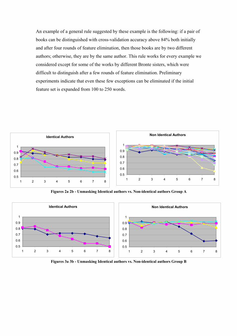
An example of a general rule suggested by these example is the following: if a pair of
books can be distinguished with cross-validation accuracy above 84% both initially
and after four rounds of feature elimination, then those books are by two different
authors; otherwise, they are by the same author. This rule works for every example we
considered except for some of the works by different Bronte sisters, which were
difficult to distinguish after a few rounds of feature elimination. Preliminary
experiments indicate that even these few exceptions can be eliminated if the initial
feature set is expanded from 100 to 250 words.
Identical Authors
0.5
0.6
0.7
0.8
0.9
1
1 2 3 4 5 6 7 8
Non Identical Authors
0.5
0.6
0.7
0.8
0.9
1
1 2 3 4 5 6 7 8
Figures 2a 2b - Unmasking Identical authors vs. Non-identical authors Group A
Identical Authors
0.5
0.6
0.7
0.8
0.9
1
1 2 3 4 5 6 7 8
Non Identical Authors
0.5
0.6
0.7
0.8
0.9
1
1 2 3 4 5 6 7 8
Figures 3a 3b - Unmasking Identical authors vs. Non-identical authors Group B

Identical Authors
0.5
0.6
0.7
0.8
0.9
1
1 2 3 4 5 6 7 8
Non Identical Authors
0.5
0.6
0.7
0.8
0.9
1
1 2 3 4 5 6 7 8
Figures 4a 4b - Unmasking Identical authors vs. Non-identical authors Group C
Identical Authors
0.5
0.6
0.7
0.8
0.9
1
1 2 3 4 5 6 7 8
Non Identical Authors
0.5
0.6
0.7
0.8
0.9
1
1 2 3 4 5 6 7 8
Figures 5a 5b - Unmasking Identical authors vs. Non-identical authors Group D
5. Conclusions
We have suggested a new approach to exploiting text categorization methods for
solving the problem of authorship confirmation. Our approach is limited to cases
where the work to be classified is of sufficient length that it can be chunked into a
significant number of reasonably long samples. (All the works we considered were of
length at least 25000 words.)
The heart of the approach is the “unmasking” process, which is a type of robustness
test: if texts remain distinguishable as the best discriminators are eliminated, they are
very likely by different authors. We have thus far assembled anecdotal evidence in
support of the effectiveness of the technique. It remains for ongoing work to refine
and test the hypothesis on a large out-of-sample test set.

6. Bibliography
[1] Sebastiani, F. (2002). Machine learning in automated text categorization, ACM Computing Surveys 34 (1), pp. 1-45
[2] Mosteller, F. and Wallace, D. L. (1964). Inference and Disputed Authorship: The Federalist. Reading, Mass. : Addison Wesley, 1964.
[3] Matthews, R. and Merriam, T. (1993). Neural computation in stylometry : An application to the works of Shakespeare and Fletcher. Literary and Linguistic computing, 8(4):203-209.
[4] Holmes, D. (1998). The evolution of stylometry in humanities scholarship, Literary and Linguistic Computing, 13, 3, 1998, pp. 111-117.
[5] Argamon, S., M. Koppel, G. Avneri (1998). Style-based text categorization: What newspaper am I reading?, in Proc. of AAAI Workshop on Learning for Text Categorization, 1998, pp. 1-4
[6] Stamatatos, E., N. Fakotakis & G. Kokkinakis, (2001). Computer-based authorship attribution without lexical measures, Computers and the Humanities 35, pp. 193—214.
[7] de Vel, O., A. Anderson, M. Corney and George M. Mohay (2001). Mining e-mail content for author identification forensics. SIGMOD Record 30(4), pp. 55-64
[8] Kivinen, J., M. Warmuth, (1997). Additive versus exponentiated gradient updates for linear prediction, Information and Computation, 132, 1, 1997, pp. 1-64.
[9] Dagan, I., Y. Karov, D. Roth (1997), Mistake-driven learning in text categorization, in EMNLP-97: 2nd Conf. on Empirical Methods in Natural Language Processing, 1997, pp. 55-63.
[10] Joachims, T. (1998) Text categorization with support vector machines: learning with many relevant features. In Proc. 10th European Conference on Machine Learning ECML-98, pages 137-142, 1998.
Mapping Dependencies Trees: An Applicationto Question Answering∗
Vasin Punyakanok Dan Roth Wen-tau YihDepartment of Computer Science
University of Illinois at Urbana-Champaign{punyakan, danr, yih}@cs.uiuc.edu
Abstract
We describe an approach for answer selection in a free form questionanswering task. In order to go beyond the key-word based matching in se-lecting answers to questions, one would like to incorporate both syntacticand semantic information in the question answering process. We achievethis goal by representing both questions and candidate passages using de-pendency trees, and incorporating semantic information such as named en-tities in this representation. The sentence that best answers a question isdetermined to be the one that minimizes the generalized edit distance be-tween it and the question tree, computed via an approximate tree matchingalgorithm. We evaluate the approach on question-answer pairs taken fromprevious TREC Q/A competitions. Preliminary experiments show its poten-tial by significantly outperforming common bag-of-word scoring methods.
1 Introduction
Open-domain natural language question answering (Q/A) is achallenging task innatural language processing which has received significantattention in the last fewyears [11, 12, 13]. In the Text REtrieval Conference (TREC) question answeringcompetition, for example, given a free form query like “What was the largest
∗This research is supported by NSF grants ITR-IIS-0085836, ITR-IIS-0085980 and IIS-9984168 and an ONR MURI Award.
1
crowd to ever come see Michael Jordan?” [13], the system can access a largecollection of newspaper articles in order to find the exact answer, e.g. “62,046”,along with a short sentence that supports it being the answer.
The overall tasks is very difficult even for fairly simple question of the typeexemplified above. A complete Q/A, requires the ability to 1)analyze questions(question analysis) in order to determine what is the question about [7], 2) retrievepotential candidate answers from the given collection of articles, and 3) determinethe final candidate that answers the question. This work concerns with the laststage only. That is, we assume that a set of candidate answersis already given,and we aim at choosing the correct candidate.
We view the problem as that of evaluating thedistance between a question andeach of their answer candidates. The candidate that has the lowest distance to thequestion is selected as the final answer. The simple bag-of-word technique doesnot perform well in this case as shown in the following example taken from [6].
What is the fastest car in the world?
The candidate answers are:
1. The Jaguar XJ220 is the dearest (415000 pounds),fastest (217mph) and most sought after car in the world.
2. ...will stretch Volkswagen’s lead in the world’sfastest growing vehicle market.
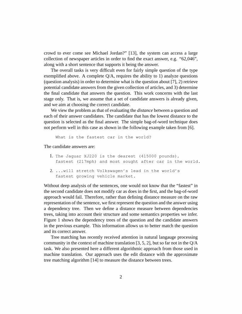
Without deep analysis of the sentences, one would not know that the “fastest” inthe second candidate does not modify car as does in the first, and the bag-of-wordapproach would fail. Therefore, rather than defining distance measure on the rawrepresentation of the sentence, we first represent the question and the answer usinga dependency tree. Then we define a distance measure between dependenciestrees, taking into account their structure and some semantics properties we infer.Figure 1 shows the dependency trees of the question and the candidate answersin the previous example. This information allows us to better match the questionand its correct answer.
Tree matching has recently received attention in natural langauge processingcommunity in the context of machine translation [3, 5, 2], but so far not in the Q/Atask. We also presented here a different algorithmic approach from those used inmachine translation. Our approach uses the edit distance with the approximatetree matching algorithm [14] to measure the distance between trees.
2
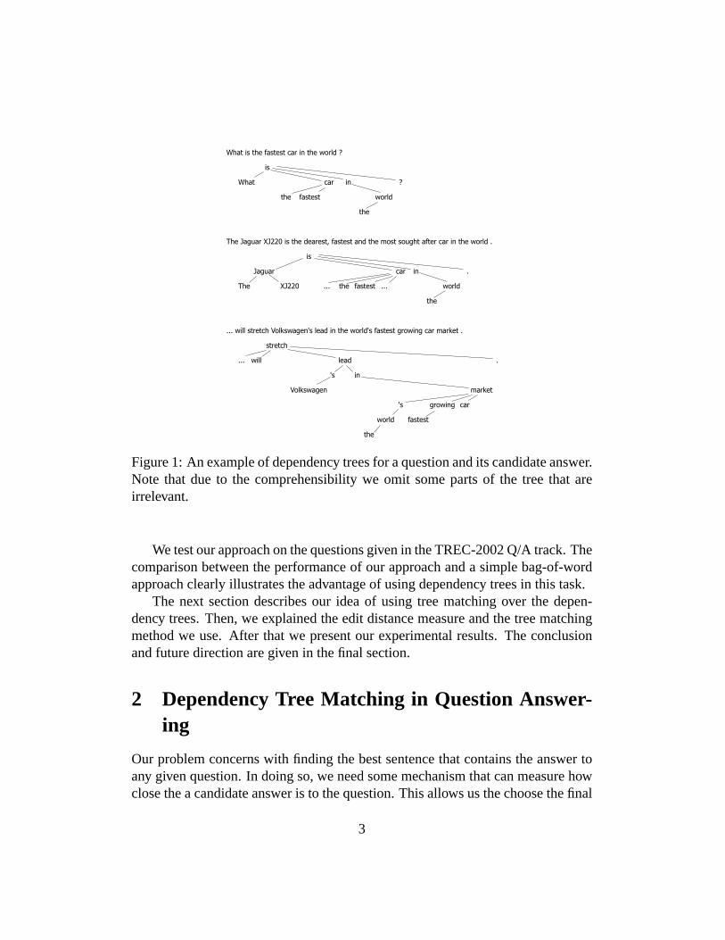
Figure 1: An example of dependency trees for a question and its candidate answer.Note that due to the comprehensibility we omit some parts of the tree that areirrelevant.
We test our approach on the questions given in the TREC-2002 Q/Atrack. Thecomparison between the performance of our approach and a simple bag-of-wordapproach clearly illustrates the advantage of using dependency trees in this task.
The next section describes our idea of using tree matching over the depen-dency trees. Then, we explained the edit distance measure and the tree matchingmethod we use. After that we present our experimental results. The conclusionand future direction are given in the final section.
2 Dependency Tree Matching in Question Answer-ing
Our problem concerns with finding the best sentence that contains the answer toany given question. In doing so, we need some mechanism that can measure howclose the a candidate answer is to the question. This allows us the choose the final
3

answer which is the one that matches the most closely to the question.To achieve this, we look at the problem in two levels. First, we need a rep-
resentation of the sentences that allows us to capture useful information in orderto accommodate the matching process. Second, we need an efficient matchingprocess to work on the chosen representation.
At the first level, the representation should be able to capture both the syntacticand semantic information of a sentence. To capture the syntactic information, werepresent questions and answers with their dependency trees which allows us tosee clearly the syntactic relations between words in the sentences. Using trees alsoallows us to flexibly incorporate other information including semantic knowledge.By allowing each node in the tree to contain more than just the surface form of itscorresponding word, we can add semantic information, e.g. what type of namedentities the word belongs, synonyms of the words, or other related words, to thenode. Moreover, each node may be generalized to contain a larger unit than aword such as a phrase or a named entity.
With an appropriate representation, the only work left is tofind the matchingbetween nodes in the question and the answer in consideration. In doing so, weuse the approximate tree matching which we explain in the next section. Formallyspeaking, we assume for each questionqi, a collection of candidate answers,Ai ={a1, a2, . . . , ani
}, each of which is a sentence, is given. We output as the finalanswer for theqi,
ai = arg mina∈Ai
DR(qi, a),
whereDR returns the minimum approximate tree matching.
3 Edit Distance and Approximate Tree Matching
We use approximate tree matching [14] in order to decide how similar any givenpair of trees are. We first introduce the edit distance [10] which is the distancemeasure used as the matching criteria. Then, we explain exactly how this measureis used in the approximate tree matching problem.
We recapture here the standard definition that was introduced by [10] and [14].We consider ordered labeled trees in which each node is labeled by some infor-mation and the order from left to right of its children is important. Edit distancemeasures the cost of doing a sequence of operations that transforms an orderedlabeled tree to another. The operations include deleting a node, inserting a node,and changing a node. Figure 2 illustrate what effect these operations have. Specif-
4
ically, when a noden is deleted, its children will be attached to the parent ofn.Insertion is the inverse of the deletion. Changing a node is toalter its label. Eachoperation is associated with some cost. A cost of a sequence of operations isthe summation of the costs of each operation. We are interested in finding theminimum cost sequence that edits a tree to another.
Figure 2: Effect of delete, insert, and change operations
Formally speaking, we represent an operation with a pair(a, b) wherea repre-sents the node to be edited andb is its result. We use(a, Λ) and(Λ, b) to representdelete and insert operation respectively. Each operation(a, b) 6= (Λ, Λ) is associ-ated with a nonnegative costγ(a → b). The cost of a sequence of operationsS =〈s1, s2, . . . , sk〉 is γ(S) =
∑k
i=1 γ(si). Given a treeT , we denotes(T ) as the treeresulting from applying operations onT , andS(T ) = sk(sk−1(. . . (s1(T )) . . . )).Given two treesT1 andT2, we would like to find
δ(T1, T2) = min{γ(S)|S(T1) = T2}
If the cost satisfies triangularity property, that isγ(a → c) 6 γ(a → b) +γ(b → c)∀a, b, c, then [10] showed that the minimum costδ(T1, T2) is a minimumcost of a mapping. A mappingM from T1 to T2 is a set of integer pairs satisfyingthe following properties. LetT [i] representith node of the treeT in any givenorder,N1 andN2 be the numbers of nodes inT1 andT2 respectively.
5

1. For any pair(i, j) ∈ M , 1 6 i 6 N1 and1 6 j 6 N2.
2. For any pairs(i1, j1) and(i2, j2) ∈ M ,
(a) i1 = i2 if and only if j1 = j2,
(b) T1[i1] is to the left ofT1[i2] if and only if T2[j1] is to the left ofT2[j2],
(c) T1[i1] is to an ancestor ofT1[i2] if and only if T2[j1] is an ancestor ofT2[j2].
The cost of a mappingM is
γ(M) =∑
(i,j)∈M
γ(T1[i] → T2[j]) +∑
(i,j)∈I
γ(T1[i] → Λ) +∑
(i,j)∈J
γ(Λ → T2[j]),
whereI is the set of index of nodes inT1 that is not mapped byM andJ is thatof nodes inT2.
In general, we can use edit distance to decide how similar anygive pair oftrees are. However, in matching question and answer sentences in the questionanswering domain, an exact answer to a question may reside only as a clause ora phrase in a sentence, not the whole sentence itself. Therefore, matching thequestion with the whole candidate sentence may result in poor match even thoughthe sentence contain the correct answer. Approximate tree matching allows us tomatch question with only some parts of the sentence not a whole. Specifically,there is no additional cost if some subtrees of the answer aredeleted.
Formally speaking, LetT1 andT2 be two trees to match. A forestS of a treeT is a set of subtrees inT such that all subtrees inS are disjoint, andT\S is thenew tree resulting from cutting all subtrees inS from T . Let S(T ) represent theset of all possible forests ofT . The approximate tree matching betweenT1 andT2
is to find:DR(T1, T2) = min
S∈S(T2)δ(T1, T2\S)
[14] gives an efficient dynamic programming based algorithmto compute theapproximate tree matching.
We note here that although the cost functions that we use in our experiments donot satisfy the triangularity property, this does not affect the underlying theories ofthe algorithm. The property is needed only in the proof of therelation between theminimum distance edit operation sequence and the minimum cost mapping. Sincewe are directly interested in finding the mapping not the operation sequence, thealgorithm correctly works for us.
6

4 Experiment
We experimented on 500 questions given in TREC-2002 Q/A competition. Therewere 46 questions that had no correct answer. The correct answers for each ques-tion, if any, were given along with the answers returned by all participants afterthe completion of the competition. We, therefore, built ourcandidate pool foreach question from its correct answers and all answers returned by all participantsto the question. In some sense, this made the problem harder for our answer se-lector. Normally, an answer selection process is evaluatedbased on the candidatepool built from the correct answer and the output from an information retrievalengine. However, our candidate pool contained those incorrect answers made byother systems; hence, we need to be more precise.
Since sentence structure might be quite different from the question, we refor-mulated the question in simple statement form using simple heuristics rules. Inthis transformation, the question word (e.g.what, when, or where) was replacedwith a special token*ANS*. Below is an example of this transformation.
Where is Devil’s Tower?Devil’s Tower is in *ANS*
Each sentence was preprocessed first by a SNoW-based part-of-speech tag-ger [4]. Then, the automatic full parser [1] was run to produce the parse trees.Since this parser also output the head word of each constituent, we could directlyconvert the parse trees to their corresponding dependency tree by simply takingthe head word as the parent. Moreover, we extracted named-entity informationwith the named-entity recognizer used in [9]. In addition, for each question, wealso ran a question classifier [7] which predicted the type ofthe answers expectedby the question.
After the answer was found, the document id that contained the answer wasreturned. We counted as correct if the returned document id matched that of thecorrect answer.
We defined three types of cost functions, namely, delete, insert and change, asshown in Figure 3. The stop word list contained some of very common word thatwould not be very meaningful, e.g. the article such as “a”, “an”, “the”. The wordlemma forms were extracted using WordNet [8].
We compared our approach with a simple bag-of-word strategy. In this simpleapproach, we measured the similarity between a question anda candidate answerwith the number of common words, either in their surface forms or lemma forms,
7

1. delete:
if a is a stop word,γ(a → Λ) = 5,
elseγ(a → Λ) = 200.
2. insert:
if a is a stop word,γ(Λ → a) = 200,
elseγ(Λ → a) = 5.
3. change:
if a is *ANS*,
if b matches the expected answer type,γ(a → b) = 5,
elseγ(a → b) = 200,
else
if word a is identical to wordb, γ(a → b) = 0,
else ifa andb have the same lemma form,γ(a → b) = 1,
elseγ(a → b) = 200.
Figure 3: The definition of cost functions
between the question and the answer divided by the length of that answer. Thefinal answer was the one that produced the highest similarity.
Note that the evaluation method we used here is different from that in TREC-2002 Q/A competition. In TREC, an answer produced by a system consists of theanswer key and the document that supports the answer. The answer is consideredcorrect only when both the answer key and the supporting document are correct.Since our system does not provide the answer key, we relax theevaluation ofour system by finding only the correct supporting document. However, this doesnot greatly simplify the task as the harder part of answer selection is to find thecorrect supporting document. The answer key may be extracted later with someheuristic rules. Also, in practice, a user who uses a Q/A system is very unlikelyto believe the system without a correct supporting document. Even though thesystem does not provide a correct answer key, the user can easily find that given acorrect supporting document at hand.
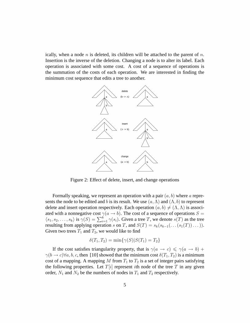
The result is shown in Table 1. It shows the large improvementof using de-
8
pendency tree over the simple bag-of-word strategy.
Table 1: The comparison of the performance of the approximate tree matchingapproach and the simple bag-of-word. The last column shows the percentage overonly the 454 questions that have an answer.
CorrectMethod # % %(454)Tree Matching 183 36.60 40.31Bag-of-Word 131 26.20 28.85
5 Conclusion
We develop an approach to apply the approximate tree matching algorithm [14]to the Q/A problem. This approach allows us to incorporate dependency trees, auseful syntactic information, in the decision process. In addition, we incorporatesome semantic information such as named entity in our approach.
We evaluate our approach on the TREC-2002 questions, and the result clearlyillustrate the potential of our approach over the common bag-of-word strategy.
In the future we plan to investigate how to use more semantic informationsuch as synonyms and related words in our approach. Moreover, each node ina tree represents only a word in a sentence, and we believe that by appropriatelycombining nodes into a meaningful phrase may allow our approach perform better.Finally, we plan to use some learning technique to learn the cost functions whichare manually defined now.
References
[1] M. Collins. Three generative, lexicalised models for statistical parsing. In Proceed-ings of the 35th Annual Meeting of the Association of Computational Linguistics,pages 16–23, Madrid, Spain, 1997.
[2] Y. Ding, D. Gildea, and M. Palmer. An algorithm for word-level alignment of par-allel dependency trees. InThe 9th Machine Translation Summit of InternationalAssociation of Machine Translation, New Orleans, LA, 2003.
9
[3] J. Eisner. Learning non-isomorphic tree mappings for machine translation. In Pro-ceedings of the 41st Annual Meeting of the Association for Computational Linguis-tics (companion volume), Supporo, Japan, July 2003.
[4] Y. Even-Zohar and D. Roth. A sequential model for multi-class classification. InProceedings of 2001 Conference on Empirical methods in Natural Language Pro-cessing, Pittsburgh, PA, 2001.
[5] D. Gildea. Loosely tree-based alignment for machine translation. InProceedings ofthe 41st Annual Meeting of the Association of Computational Linguistics (ACL-03),Supporo, Japan, 2003.
[6] S. Harabagiu and D. Moldovan. Open-domain textual question answering. In Tu-turial of the Second Meeting of the North American Chapter of the Association forComputational Linguistics, 2001.
[7] X. Li and D. Roth. Learning question classifiers. InCOLING 2002, The 19thInternational Conference on Computational Linguistics, pages 556–562, 2002.
[8] G. Miller, R. Beckwith, C. Fellbaum, D. Gross, and K.J. Miller. Wordnet:An on-linelexical database.International Journal of Lexicography, 3(4):235–312, 1990.
[9] D. Roth, G. K. Kao, X. Li, R. Nagarajan, V. Punyakanok, N. Rizzolo, W-T. Yih,C. Ovesdotter, and L. Moran. Learning components for a question-answering sys-tem. InProceedings of The Tenth Text REtrieval Conference (TREC 2001), Gaithes-burg, Maryland, 2001.
[10] K. Tai. The tree-to-tree correction problem.Journal of the Association for Comput-ing Machinery, 26(3):422–433, July 1979.
[11] E. Voorhees. Overview of the trec-9 question answering track. In The Ninth TextRetrieval Conference (TREC-9), pages 71–80. NIST SP 500-249, 2000.
[12] E. Voorhees. Overview of the trec 2001 question answering. InThe Tenth TextRetrieval Conference (TREC 2001), pages 42–51. NIST SP 500-250, 2001.
[13] E. Voorhees. Overview of the trec 2002 question answering. InThe Eleventh TextRetrieval Conference (TREC 2002). NIST SP 500-251, 2002.
[14] K. Zhang and D. Shasha. Simple fast algorithms for the editing distancebetweentrees and related problems.SIAM Journal on Computing, 18(6):1245–1262, Decem-ber 1989.
10

A Linear Programming Formulation for Global Inferencein Natural Language Tasks∗
Dan Roth Wen-tau YihDepartment of Computer Science
University of Illinois at Urbana-Champaign{danr, yih }@uiuc.edu
Abstract
The typical processing paradigm in natural language processing is the “pipeline” approach,where learners are being used at one level, their outcomes are being used as features for asecond level of predictions and so one. In addition to accumulating errors, it is clear thatthe sequential processing is a crude approximation to a process in which interactions occuracross levels and down stream decisions often interact with previous decisions.This work develops a general approach to inference over the outcomes of predictors in thepresence of general constraints. It allows breaking away from the pipeline paradigm byperforming global inference over the outcome of different predictors — potentially learnedand evaluated given only partial information — along with domain and task specific con-straints on the outcomes of the predictors. At the inference level, the existence of mutualconstraints on simultaneous outcomes of predictors results in modifying these predictionsto optimize global and task specific constraints.We develop a linear programming formulation for this problem and evaluate it in the contextof simultaneously learning named entities and relations between. Our approach allows usto efficiently incorporate domain and task specific constraints at decision time, resulting insignificant improvements in the accuracy and the “human-like” quality of the inferences.
1 Introduction
Natural language decisions often depend on the outcomes of several different but mutually dependent predic-tions with respect to the input. These predictions need to respect some constraints that could arise from thenature of the data or from domain or task specific conditions, hence require a level of inference on top the pre-dictions. As an example from the visual processing domain that exemplifies this point, consider the problemof counting the number of people in an image, where people can be partly occluded; a large number of “bodypart detectors” and scene interpretations predictors come into play, and some inference procedures takesthese into account in making the final decision. Similarly, interpreting natural language sentences requiresa multitude of abstractions and context dependent disambiguations that depend on each other in intricateways. Efficient solutions to problems of these sort have been given when the constraints on the predictors aresequential. Variations of HMMs, conditional models and sequential variations of random Markov fields allprovide efficient solutions [1, 2].
However, in many important situations, the structure of the problem is more general, resulting in a computa-tionally intractable problem. Problems of these sorts have been studied in computer vision, where inferenceis typically done over low level measurements rather than over higher level predictors [3, 4]. In the contextof natural language, the typical processing paradigm is the “pipeline” approach, where learners are beingused at one level, and their outcomes are being used as features for a second level of predictions and so one.For example, it is typical to learn apart-of-speechtagger, evaluate it and use the outcome as features in the
∗This research is supported by NSF grants ITR-IIS-0085836, ITR-IIS-0085980 and IIS-9984168 and an ONR MURIAward.
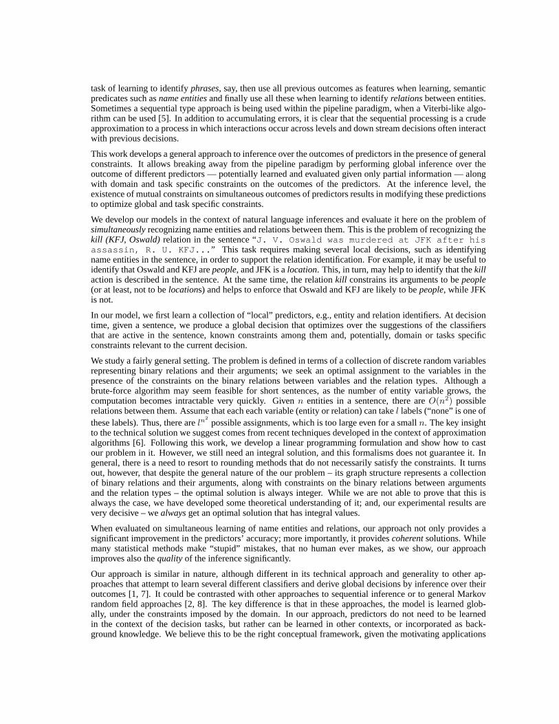
task of learning to identifyphrases, say, then use all previous outcomes as features when learning, semanticpredicates such asname entitiesand finally use all these when learning to identifyrelationsbetween entities.Sometimes a sequential type approach is being used within the pipeline paradigm, when a Viterbi-like algo-rithm can be used [5]. In addition to accumulating errors, it is clear that the sequential processing is a crudeapproximation to a process in which interactions occur across levels and down stream decisions often interactwith previous decisions.
This work develops a general approach to inference over the outcomes of predictors in the presence of generalconstraints. It allows breaking away from the pipeline paradigm by performing global inference over theoutcome of different predictors — potentially learned and evaluated given only partial information — alongwith domain and task specific constraints on the outcomes of the predictors. At the inference level, theexistence of mutual constraints on simultaneous outcomes of predictors results in modifying these predictionsto optimize global and task specific constraints.
We develop our models in the context of natural language inferences and evaluate it here on the problem ofsimultaneouslyrecognizing name entities and relations between them. This is the problem of recognizing thekill (KFJ, Oswald)relation in the sentence “J. V. Oswald was murdered at JFK after hisassassin, R. U. KFJ... ” This task requires making several local decisions, such as identifyingname entities in the sentence, in order to support the relation identification. For example, it may be useful toidentify that Oswald and KFJ arepeople, and JFK is alocation. This, in turn, may help to identify that thekillaction is described in the sentence. At the same time, the relationkill constrains its arguments to bepeople(or at least, not to belocations) and helps to enforce that Oswald and KFJ are likely to bepeople, while JFKis not.
In our model, we first learn a collection of “local” predictors, e.g., entity and relation identifiers. At decisiontime, given a sentence, we produce a global decision that optimizes over the suggestions of the classifiersthat are active in the sentence, known constraints among them and, potentially, domain or tasks specificconstraints relevant to the current decision.
We study a fairly general setting. The problem is defined in terms of a collection of discrete random variablesrepresenting binary relations and their arguments; we seek an optimal assignment to the variables in thepresence of the constraints on the binary relations between variables and the relation types. Although abrute-force algorithm may seem feasible for short sentences, as the number of entity variable grows, thecomputation becomes intractable very quickly. Givenn entities in a sentence, there areO(n2) possiblerelations between them. Assume that each each variable (entity or relation) can takel labels (“none” is one ofthese labels). Thus, there areln
2possible assignments, which is too large even for a smalln. The key insight
to the technical solution we suggest comes from recent techniques developed in the context of approximationalgorithms [6]. Following this work, we develop a linear programming formulation and show how to castour problem in it. However, we still need an integral solution, and this formalisms does not guarantee it. Ingeneral, there is a need to resort to rounding methods that do not necessarily satisfy the constraints. It turnsout, however, that despite the general nature of the our problem – its graph structure represents a collectionof binary relations and their arguments, along with constraints on the binary relations between argumentsand the relation types – the optimal solution is always integer. While we are not able to prove that this isalways the case, we have developed some theoretical understanding of it; and, our experimental results arevery decisive – wealwaysget an optimal solution that has integral values.
When evaluated on simultaneous learning of name entities and relations, our approach not only provides asignificant improvement in the predictors’ accuracy; more importantly, it providescoherentsolutions. Whilemany statistical methods make “stupid” mistakes, that no human ever makes, as we show, our approachimproves also thequalityof the inference significantly.
Our approach is similar in nature, although different in its technical approach and generality to other ap-proaches that attempt to learn several different classifiers and derive global decisions by inference over theiroutcomes [1, 7]. It could be contrasted with other approaches to sequential inference or to general Markovrandom field approaches [2, 8]. The key difference is that in these approaches, the model is learned glob-ally, under the constraints imposed by the domain. In our approach, predictors do not need to be learnedin the context of the decision tasks, but rather can be learned in other contexts, or incorporated as back-ground knowledge. We believe this to be the right conceptual framework, given the motivating applications

in NLP and computer vision described above. This way, our technical approach allows the incorporationof constraints into decisions in a dynamic fashion and can therefore support task specific inferences. Thesignificance of this is clearly shown in our experimental results.
2 The Relational Inference Problem
We consider the relational inference problem within thereasoning with classifiersparadigm [9]. Thisparadigm investigates decisions that depend on the outcomes of several different but mutually dependentclassifiers. The classifiers’ outcomes need to respect some constraints that could arise from the sequential na-ture of the data or other domain specific conditions, thus requiring a level of inference on top the predictions.In this way, variables considered here are in fact outcomes of learned classifiers, learned over a large numberof variables (features) that are abstracted away here, since they are not of interest for the inference process.All the information in these is contained in the classifiers’ outcome.
We study a specific but fairly general instantiation of this problem, motivated by the problem of recognizingnamed entities (e.g., persons, locations, organization names) and relations between them (e.g. workfor,locatedin, live in). We consider a setsV which consists of two types of variablesV = E ∪ R. The first setof variablesE = {E1, E2, · · · , En} rangesLE . The value (called “label”) assigned toEi ∈ E is denotedfEi ∈ LE . The second set of variablesR = {Rij}{1≤i,j≤n;i 6=j} is viewed as binary relations overE .Specifically, for each pair of entitiesEi andEj , i 6= j, we useRij andRji to denote the (binary) relations(Ei, Ej) and(Ej , Ei) respectively. The set of labels of relations isLR and the label assigned to relationRij ∈ R is fRij
∈ LR.
Apparently, there exists some constraints on the labels of corresponding relation variables, and entity vari-ables. For instance, if the relation islive in, then the first entity should be aperson, and the second entityshould be alocation. The correspondence between the relation and entity variables can be represented by abipartite graph. Each relation variableRij is connected to its first entityEi , and second entityEj . We useN 1 andN 2 to denote the entity variables of a relationRij . Specifically,Ei = N 1(Rij) andEj = N 2(Rij)
In addition, we define a set of constraints on the outcomes of the variables inV. C1 : LE ×LR → {0, 1} con-straints values by the first argument of relations.C2 is defined similarly and constrains the second argumenta relation can take. For example, (born in, person) is in C1 but not inC2 because the first entity of relationborn in has to be apersonand the second entity can only be alocation instead of aperson. Note that whilewe define the constraints here as Boolean, our formalisms in fact allows for stochastic constraints. Also notethat we can define a large number of constraints, such asCR : LR × LR → {0, 1} which constrain typesof relations, etc. In fact, as will be clear in Sec. 3 the language for defining constraints is very rich – linearequations overV.
We exemplify the framework using the problem of simultaneous recognition or named entities and relationsin sentences. Briefly, we assume a learning mechanism that can recognize entity phrases in sentences, basedon local contextual features. Similarly, we assume a learning mechanism that can recognize the semanticrelation between two given phrases in a sentence. We seek an inference algorithm that can produce a coherentlabeling of entities and relations in a given sentence, satisfying, as best as possible the recommendation ofthe entity and relation classifiers, but also satisfying natural constraints that exist on whether specific entitiescan be the argument of specific relations, whether two relations can occur together at the same time, or anyother information that might be available at the inference time (e.g., Suppose it is known that entity A and Brepresent the same location; one may like to incorporate an additional constraint that prevents an inference ofthe type: “C lives in A; C does not live in B”).
We note that a large number of problems can be modeled this way. Examples include problems such aschunking sentences [1], coreference resolution and sequencing problems in computational biology. In fact,each of the components of our problem here, the separate task of recognizing named entities in sentences andthe task of recognizing semantic relations between phrases can be modeled this way. However, our goal hereis specifically to consider interacting problems at different levels, resulting in a more complex constraintsamong them, and exhibit the power of our method.
The most direct way to formalize our inference problem is via the formalism of Markov Random Field (MRF)

theory [10]. Rather than doing that, for computational reasons, we first use a fairly standard transformation ofMRF to a discrete optimization problem (see [11] for details). Specifically, under weak assumptions we canview the inference problem as the following optimization problem, which aims to to minimize the objectivefunction that is the sum of the following two cost functions.
Assignment cost: The costs of deviating from the assignment of the variablesV given by the classifiers.The specific cost function we use is defined as follows: Letl be the label assigned to variableu ∈ V. If themarginal probability estimation isp = P (fu = l), then the assignment costcu(l) is− log p.
Constraints cost: The cost imposed by breaking constraints between neighboring nodes. The specificcost function we use is defined as follows: Consider two entity nodesEi, Ej and its corresponding relationnodeRij ; that is,Ei = N 1(Rij) andEj = N 2(Rij). The constraint cost indicates whether the labelsare consistent with the constraints. In particular, we use:d1(fEi
, fRij) is 0 if (fRij
, fEi) ∈ C1; otherwise,
d1(fEi, fRij
) is∞ 1. Similarly, we used2 to force the consistency of the second argument of a relation.
Since we are seeking a most probable global assignment that satisfies the constraints, therefore, the overallcost function we optimize, for a global labelingf of all variables is:
C(f) =∑u∈V
cu(fu) +∑
Rij∈R
[d1(fRij
, fEi) + d2(fRij
, fEj)]
(1)
3 A Computational Approach to Relational Inference
Unfortunately, it is not hard to see that the optimization problem 1 is computationally intractable even whenplacing assumptions on the cost function [11].
The computational approach we adopt is based on alinear programmingformulation of the problem. Wefirst provide an integer linear programming formulation to Eq. 1, and thenrelax it to a linear programmingproblem. This Linear Programming Relaxation (LPR) [12, 13] technique, in general, might find non-integersolutions. Therefore, to “round” the solutions to integer solutions is needed. Under some assumptions on thecost function, which do not hold in our case, there exist rounding procedures that guarantee some optimality[11, 6]. However, such rounding procedures do not always exist. We discuss the issue of integer solutionsto linear programs and provide evidence that for our target problems, rounding is not required – the linearprogram always has an optimal integer solution.
Our linear programming formulation is based on the methods proposed by [6]. Since our objective function(Eq.1) is not a linear function in terms of the labels, we introduce new binary decision variables to representdifferent possible assignments to each original variable; we then represent the objective function as a linearfunction of these binary variables.
Let x{u,i} be a{0, 1}-variable, defined to be1 if and only if variableu is labeledi, whereu ∈ E , i ∈ LE oru ∈ R, i ∈ LR. For example,x{E1,2} = 1 when the label of entityE1 is 2; x{R23,3} = 0 when the label ofrelationR23 is not 3. Letx{Rij ,r,Ei,e1} be a{0, 1}-variable indicating whether relationRij is assigned labelr and its first argumentEi is assigned labele1. For instance,x{R12,1,E1,2} = 1 means the label of relationR12 is 1andthe label of its first argumentE1 is 2. Similarly,x{Rij ,r,Ej ,e2} = 1 indicates thatRij is assignedlabelr and its second argumentEj is assigned labele2. With these definitions, the optimization problem canbe represented as the following integer programming problem.
min∑E∈E
∑e∈LE
cE(e) · x{E,e} +∑R∈R
∑r∈LR
cR(r) · x{R,r}
+∑
Ei,Ej∈EEi 6=Ej
[ ∑r∈LR
∑e1∈LE
d1(r, e1) · x{Rij ,r,Ei,e1} +∑
r∈LR
∑e2∈LE
d2(r, e2) · x{Rij ,r,Ej ,e2}
]
1In practice, we use a very large number (915).
subject to: ∑e∈LE
x{E,e} = 1 ∀E ∈ E (2)
∑r∈LR
x{R,r} = 1 ∀R ∈ R (3)
x{E,e} =∑
r∈LR
x{R,r,E,e} ∀R ∈ {R : E = N 1(R) or R : E = N 2(R)} (4)
x{R,r} =∑
e∈LE
x{R,r,E,e} ∀E = N 1(R) or E = N 2(R) (5)
x{E,e} ∈ {0, 1} ∀E ∈ E , e ∈ LE (6)
x{R,r} ∈ {0, 1} ∀R ∈ R, r ∈ LR (7)
x{R,r,E,e} ∈ {0, 1} ∀R ∈ R, r ∈ LR, E ∈ E , e ∈ LE (8)
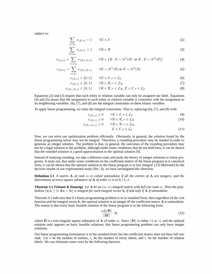
Equations (2) and (3) require that each entity or relation variable can only be assigned one label. Equations(4) and (5) assure that the assignment to each entity or relation variable is consistent with the assignment toits neighboring variables. (6), (7), and (8) are the integral constraints on these binary variables.
To apply linear programming, we relax theintegralconstraints. That is, replacing (6), (7), and (8) with:
x{E,e} ≥ 0 ∀E ∈ E , e ∈ LE (9)
x{R,r} ≥ 0 ∀R ∈ R, r ∈ LR (10)
x{R,r,E,e} ≥ 0 ∀R ∈ R, r ∈ LR,
E ∈ E , e ∈ LE (11)
Now, we can solve our optimization problem efficiently. Obviously, in general, the solution found by thelinear programming solver may not be integral. Therefore, a rounding procedure may be needed in order togenerate an integer solution. The problem is that, in general, the outcomes of the rounding procedure maynot be a legal solution to the problem, although under some conditions that do not hold here, it can be shownthat the rounded solution is a good approximation to the optimal solution [6].
Instead of studying rounding, we take a different route and study the theory of integer solutions to linear pro-grams. It turns out, that under some conditions on the coefficient matrix of the linear program in it canonicalform, it can be shown that the optimal solution to the linear program is in fact integral. [13] Motivated by thedecisive results of our experimental study (Sec. 4), we have investigated this direction.
Definition 3.1 A matrix A of rank m is called unimodularif all the entries ofA are integers, and thedeterminant of every square submatrix ofA of orderm is in 0,+1,-1.
Theorem 3.1 (Veinott & Dantzig) LetA be an(m,n)-integral matrix with full row rankm. Then the poly-hedron{x|x ≥ 0;Ax = b} is integral for each integral vectorb, if and only ifA if unimodular.
Theorem 3.1 indicates that if a linear programming problem is in its standard form, then regardless of the costfunction and the integral vectorb, the optimal solution is an integer iff the coefficient matrixA is unimodular.The reason is that every basic feasible solution of the linear program is in the following form:
adj(B)||B||
· b, (12)
whereB is a non-singular square submatrix ofA of orderm. Since||B|| is either +1 or -1, and the optimalsolution only appears on basic feasible solutions, this linear programming problem can only have integersolutions.
Our linear programming formulation is in the standard form, but the coefficient matrix does not have full rowrank. Letn be the number of entities,le be the number of entity labels, andlr be the number of relationlabels. We can eliminate some rows by the following theorem.

Theorem 3.2 The coefficient matrixA of our linear programming formulation is an(n2 + 2n(n − 1)(le +lr), nle + n(n − 1)lr + 2n(n − 1)lrle) matrix, and all the entries are in (0,+1,-1). In addition, rank(A) isn2 + 2n(n− 1)(le + lr − 1) and the full rank matrixA′ can be derived by eliminating the firstn2 − 1 rowsand the last(n− 1)2 rows ofA.
After this elimination, the corresponding vectorb′ in our linear programming formulation has a nice property– the first entry is 1 and all other entries are 0.
Combining the above results, we know that if the linear programming formulation has any of the followingproperties, we will always get an optimal integer solution. (1)A′ is unimodular. (2) The first columnof adj(B′) is (a1, a2, . . . , ar)T ||B′||, whereB′ is a non singular submatrix ofA′ of order = rank(A′),r = rank(A) and allai, 1 ≤ i ≤ r, are integers. (3) The constraints in our problem forbid non integersolutions.
We find many of our problems have at least one of the above properties. For those that don’t have theproperties, by examining the coefficient matrix, we observe that the non integer solution can only happenwhen there are at least two integer solutions that also have the optimal cost. Although at this point we arestill looking for the proof, we have the following conjecture.
Conjecture 3.1 Any non integer basic feasible solutionx in our problem is a convex combination of severalinteger basic feasible solutionsy1, . . . ,yk.
Since the cost functionc, is a convex function (linear), there exists ayi(1 ≤ i ≤ k) such that thec(x) ≥ c(yi).Becausex is optimal, thereforec(x) = c(yi). Note that in practice, it is very unlikely to have two optimalsolutions. As mentioned above, none of the thousand cases we experimented requires rounding.
4 Experiments
We describe below two experiments on the problem of simultaneously recognizing entities and relations. Inthe first, we view the task as a knowledge acquisition task – we let the system read sentences and identifyentities and relations among them. Given that this is a difficult task which may require quite often informationbeyond the sentence, we consider also a “forced decision” task, in which we simulate a question answeringsituation – we ask the system, say, “who killed whom” and evaluate it on identifying correctly the relationand its arguments, given that it is known that somewhere in this sentence this relation is active. In addition,this evaluation exhibits the ability of our approach to incorporate task specific constraints at decision time.
Our experiments are based on a the TREC data set (which consists of articles from WSJ, AP, etc.) that weannotated for named entities and relations. In order to effectively observe the interaction between relationsand entities, we picked 1437 sentences that have at least one active relation. Among those sentences, thereare 5336 entities, and 19048 pairs of entities (binary relations). Entity labels include 1685persons, 1968locations, 978 organizationsand 705others. Relation labels include 406locatedin, 394 work for, 451orgBasedin, 521 live in, 268kill , and 17007none. Note that most pair of entities have no active relation atall. Therefore, relationnonesignificantly outnumbers others.
Examples of each relation label and the constraints between a relation variable and its two entity argumentsare shown as follows.
Relation Entity1 Entity2 Examplelocatedin loc loc (New York, US)work for per org (Bill Gates, Microsoft)
orgBasedin org loc (HP, Palo Alto)live in per loc (Bush, US)
kill per per (Oswald, JFK)
In order to focus on the evaluation of our inference procedure, we assume the problem ofsegmentation(orphrase detection) [14, 1] is solved, and the entity boundaries are given to us as input; thus we only concentrateon their classification.
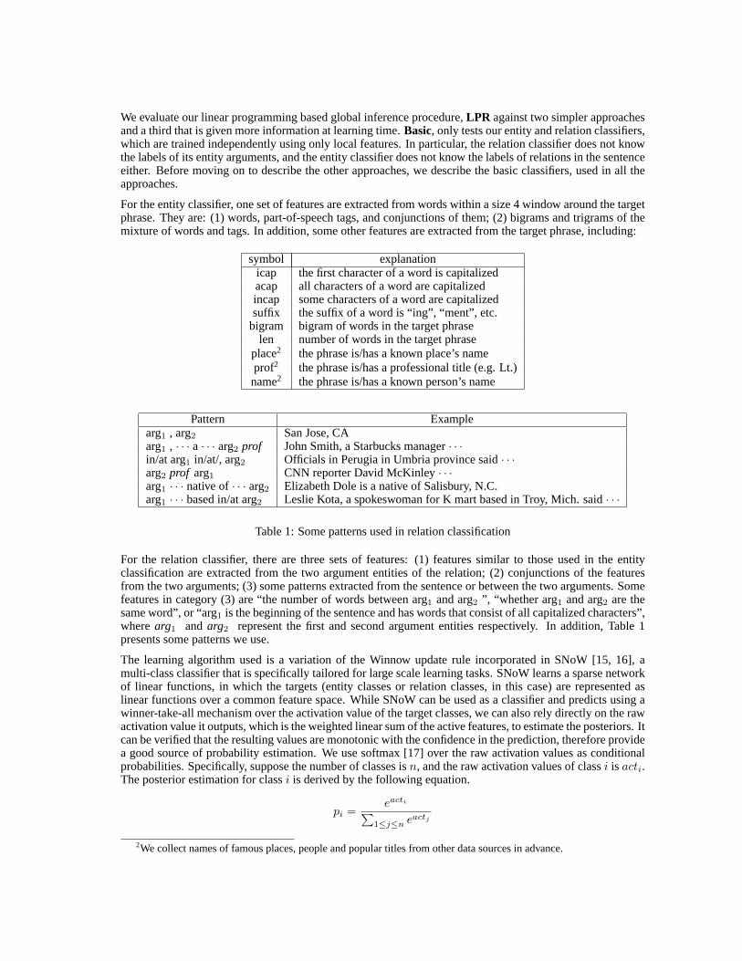
We evaluate our linear programming based global inference procedure,LPR against two simpler approachesand a third that is given more information at learning time.Basic, only tests our entity and relation classifiers,which are trained independently using only local features. In particular, the relation classifier does not knowthe labels of its entity arguments, and the entity classifier does not know the labels of relations in the sentenceeither. Before moving on to describe the other approaches, we describe the basic classifiers, used in all theapproaches.
For the entity classifier, one set of features are extracted from words within a size 4 window around the targetphrase. They are: (1) words, part-of-speech tags, and conjunctions of them; (2) bigrams and trigrams of themixture of words and tags. In addition, some other features are extracted from the target phrase, including:
symbol explanationicap the first character of a word is capitalizedacap all characters of a word are capitalizedincap some characters of a word are capitalizedsuffix the suffix of a word is “ing”, “ment”, etc.
bigram bigram of words in the target phraselen number of words in the target phrase
place2 the phrase is/has a known place’s nameprof2 the phrase is/has a professional title (e.g. Lt.)name2 the phrase is/has a known person’s name
Pattern Examplearg1 , arg2 San Jose, CAarg1 , · · · a · · · arg2 prof John Smith, a Starbucks manager· · ·in/at arg1 in/at/, arg2 Officials in Perugia in Umbria province said· · ·arg2 prof arg1 CNN reporter David McKinley· · ·arg1 · · · native of· · · arg2 Elizabeth Dole is a native of Salisbury, N.C.arg1 · · · based in/at arg2 Leslie Kota, a spokeswoman for K mart based in Troy, Mich. said· · ·
Table 1: Some patterns used in relation classification
For the relation classifier, there are three sets of features: (1) features similar to those used in the entityclassification are extracted from the two argument entities of the relation; (2) conjunctions of the featuresfrom the two arguments; (3) some patterns extracted from the sentence or between the two arguments. Somefeatures in category (3) are “the number of words between arg1 and arg2 ”, “whether arg1 and arg2 are thesame word”, or “arg1 is the beginning of the sentence and has words that consist of all capitalized characters”,wherearg1 and arg2 represent the first and second argument entities respectively. In addition, Table 1presents some patterns we use.
The learning algorithm used is a variation of the Winnow update rule incorporated in SNoW [15, 16], amulti-class classifier that is specifically tailored for large scale learning tasks. SNoW learns a sparse networkof linear functions, in which the targets (entity classes or relation classes, in this case) are represented aslinear functions over a common feature space. While SNoW can be used as a classifier and predicts using awinner-take-all mechanism over the activation value of the target classes, we can also rely directly on the rawactivation value it outputs, which is the weighted linear sum of the active features, to estimate the posteriors. Itcan be verified that the resulting values are monotonic with the confidence in the prediction, therefore providea good source of probability estimation. We use softmax [17] over the raw activation values as conditionalprobabilities. Specifically, suppose the number of classes isn, and the raw activation values of classi is acti.The posterior estimation for classi is derived by the following equation.
pi =eacti∑
1≤j≤n eactj
2We collect names of famous places, people and popular titles from other data sources in advance.

Pipeline, mimics the typical strategy in solving complex natural language problems – separating a task intoseveral stages and solving them sequentially. For example, a named entity recognizer may be trained usinga different corpus in advance, and given to a relation classifier as a tool to extract features. This approachfirst trains an entity classifier as described in thebasicapproach, and then uses the prediction of entities inaddition to other local features to learn the relation identifier. Note that although the true labels of entities areknown when training the relation identifier, this may not be the case in general NLP problems. Therefore, thepredictions of the entity classifier are used instead.
LPR, is our global inference procedure. It takes as input the constraints between a relation and its entityarguments, and the output (the estimated probability distribution of labels) of the basic classifiers. Note thatLPRmay change the predictions for either entity labels or relation labels, whilepipelinefully trusts the labelsof entity classifier, and only the relation predictions may be different from the basic relation classifier. In otherwords,LPR is able to enhance the performance of entity classification, which is impossible forpipeline.
The final approach,Omniscience, tests the conceptual upper bound of this entity/relation classification prob-lem. It also trains the two classifiers separately as thebasicapproach. However, it assumes that the entityclassifier knows the correct relation labels and, similarly, the relation classifier knows the right entity labelsas well. This additional information is then used as features in training and testing. Note that this assumptionis totally unrealistic. Nevertheless, it may give us a hint that how much a global inference can achieve.
4.1 Results
Approach person organization locationRec. Prec. F1 Rec. Prec. F1 Rec. Prec. F1
Basic 89.4 89.2 89.3 86.9 91.4 89.1 68.2 90.9 77.9Pipeline 89.4 89.2 89.3 86.9 91.4 89.1 68.2 90.9 77.9
LPR 90.4 90.0 90.2 88.5 91.7 90.1 71.5 91.0 80.1Omniscient 94.9 93.5 94.2 92.3 96.5 94.4 88.3 93.4 90.8
Table 2: Results of Entity Classification
Approach locatedin work for orgBasedinRec. Prec. F1 Q. Rec. Prec. F1 Q. Rec. Prec. F1 Q.
Basic 54.7 43.0 48.2 89.2 42.1 51.6 46.4 74.1 36.1 84.9 50.6 93.6Pipeline 51.2 51.6 51.4 88.9 41.4 55.6 47.5 76.7 36.9 76.6 49.9 94.0
LPR 53.2 59.5 56.2 100 40.4 72.9 52.0 100 36.3 90.1 51.7 100Omniscient 64.0 54.5 58.9 100 50.5 69.1 58.4 100 50.2 76.7 60.7 100
Approach live in killRec. Prec. F1 Q. Rec. Prec. F1 Q.
Basic 39.7 61.6 48.3 92.3 82.1 73.6 77.6 96.8Pipeline 42.6 62.2 50.6 90.5 83.2 76.4 79.6 96.9
LPR 41.5 68.1 51.6 100 81.3 82.2 81.7 100Omniscient 57.0 60.7 58.8 100 82.1 74.6 78.2 99.5
Table 3: Results of Relation Classification
Tables 2 & 3 show the performance of each approach inFβ=1. The results show thatLPRperforms consis-tently better thanbasicandpipeline, both in entities and relations. While we do not show it for lack of space,it enhances both recall and precision, reflected in aF1. Note thatLPRdoes not apply learning at all, but stilloutperformspipeline, which uses entity predictions as new features in learning. The results of theomniscientclassifiers reveal that there is still room for improvement. One option is to apply learning to tune a better costfunction in theLPRapproach.
One of the more significant results in our experiments, we believe, is the improvement in thequality of thedecisions. As mentioned in Sec. 1, incorporating constraints helps to avoidstupid(from a human perspec-tive) mistakes in classification. It is interesting to examine how often such mistakes happen without global

inference, and see how effectively the global inference enhances this. For this purpose, we define thequalityof the decision as follows. For an active relation of which the label is classified correctly, if both its argumententities are also predicted correctly, we count it as acoherentprediction.Quality(Q.) is then the number ofcoherentpredictions divided by the sum ofcoherentandincoherentpredictions. Since thebasicandpipelineapproaches do not have a global view of the labels of entities and relations, a certain amount of the predictionsare incoherent. Therefore, the quality is not always good. On the other hand, our global inference procedure,LPR, takes the natural constraints into account, so it never generates incoherent predictions. If the relationclassifier has the correct entity labels as features, a good learner should learn the constraints as well. As aresult, the quality ofomniscientis almost as good asLPR.
Another experiment we did is theforced decisiontest, which boosts theF1 of “kill” relation to 86.2%. Herewe consider only sentences in which the “kill” relation is active, and we force the system to determine whichof the possible relations in a sentence (i.e., which pair of entities) has this relation. This is a realistic situation(e.g., in the context of question answering) in that it adds an external constraint, not present at the time oflearning the classifiers and it evaluates the ability of our inference algorithm to cope with it. The resultsexhibit that our expectations are correct. In fact, we believe that in natural situations the number of constraintthat can apply is even larger, and observing the algorithm performs on other, specific, forced decision tasksverifies that LPR is reliable in these situation, and as shown, performs better thanomnisciencewho is givenmore information at learning time, but cannot adapt to the situation at decision time.
5 Discussion
We presented an approach for global inference in situations where decisions depend on the outcomes ofseveral different but mutually dependent classifiers whose outcomes need to respect domain or tasks specificconstraint.
We have shown that even in the presence of a fairly general constraint structure, deviating from the sequentialnature typically studied, we can develop an optimal and efficient inference procedure. Our technical approachis based on formulating the discrete inference problem as a linear program, and arguing that it admits aninteger solution. Although we have developed some theoretical understanding, our claim is based so far onlyon overwhelming experimental evidence, and an attempt to solidify it is on top of our agenda.
The key advantage of the linear programming formulation is its generality and flexibility; in particular, itsupports the ability to incorporate classifiers learned in other contexts, “hints” supplied and decision timeconstraints, and reason with all these for the best global prediction. In sharp contrast with the typically usedpipeline framework, our formulation does not blindly trust the results of some classifiers, and therefore isable to overcome mistakes made by classifiers with the help of constraints.
Our experiments have demonstrated these advantages by considering the interaction between entity and re-lation classifiers. In fact, more classifiers can be added and used within the same framework. For example,if coreference resolution is available, it is possible to incorporate it in the form of constraints that force thelabels of the co-referred entities to be the same (but, of course, allowing the global solution to reject the sug-gestion of these classifiers). Consequently, this may enhance the performance of entity/relation recognitionand, at the same time, correct possible coreference resolution errors. Another example is to use chunkinginformation for better relation identification; suppose, for example that we have available chunking informa-tion that identifies Subj+Verb and Verb+Object phrases. Given a sentence that has the verb “murder”, wemay conclude that the subject and object of this verb are in a “kill” relation. Since the chunking informationis used in the global inference procedure, this information will contribute to enhancing its performance androbustness, relying on having more constraints and overcoming possible mistakes by some of the classifiers.Moreover, in an interactive environment where a user can supply new constraints (e.g., a question answeringsituation) this framework is able to make use of the new information and enhance the performance at decisiontime, without retraining the classifiers.
As we show, our formulation supports not only improved accuracy, but also improves the ‘human-like” qualityof the decisions. We believe that it has the potential to be a powerful way for supporting natural languageinferences.

References
[1] V. Punyakanok and D. Roth. The use of classifiers in sequential inference. InNIPS-13; The 2000Conference on Advances in Neural Information Processing Systems, pages 995–1001. MIT Press, 2001.
[2] J. Lafferty, A. McCallum, and F. Pereira. Conditional random fields: Probabilistic models for segment-ing and labeling sequence data. InProc. 18th International Conf. on Machine Learning, pages 282–289.Morgan Kaufmann, San Francisco, CA, 2001.
[3] A. Levin, A. Zomet, and Yair Weiss. Learning to perceive transparency from the statistics of naturalscenes. InNIPS-15; The 2002 Conference on Advances in Neural Information Processing Systems,2002.
[4] Y. Boykov, O. Veksler, and R. Zabih. Fast approximate energy minimization via graph cuts.IEEETransactions on Pattern Analysis and Machine Intelligence, 23(11):1222–1239, November 2001.
[5] A. Ratnaparkhi. Learning to parse natural language with maximum entropy models.Machine Learning,34(1-3):151–175, 1999.
[6] C. Chekuri, S. Khanna, J. Naor, and L. Zosin. Approximation algorithms for the metric labeling problemvia a new linear programming formulation. InSymposium on Discrete Algorithms, pages 109–118,2001.
[7] Dan Klein, Joseph Smarr, Huy Nguyen, and Christopher D. Manning. Named entity recognition withcharacter-level models. In Walter Daelemans and Miles Osborne, editors,Proceedings of CoNLL-2003,pages 180–183. Edmonton, Canada, 2003.
[8] B. Tasker, A. Pieter, and D. Koller. Discriminative probabilistic models for relational data. InUncer-tainty in Artificial Intelligence: Proceedings of the Eighteenth Conference (UAI-2002), pages 485–492,San Francisco, CA, 2002. Morgan Kaufmann Publishers.
[9] D. Roth. Reasoning with classifiers. InProc. of the European Conference on Machine Learning, pages506–510, 2001.
[10] S. Li. Markov Random Field Modeling in Image Analisys. Springer-Verlag, 2001.
[11] J. Kleinberg and E. Tardos. Approximation algorithms for classification problems with pairwise rela-tionships: Metric labeling and markov random fields. InIEEE Symposium on Foundations of ComputerScience, pages 14–23, 1999.
[12] G. Sierksma.Linear and integer programming : theory and practice. Marcel Dekker, January 2001.
[13] A. Schrijver. Theory of Linear and Integer Programming. Wiley Interscience series in discrete math-matics. John Wiley & Sons, December 1986.
[14] S. P. Abney. Parsing by chunks. In S. P. Abney R. C. Berwick and C. Tenny, editors,Principle-basedparsing: Computation and Psycholinguistics, pages 257–278. Kluwer, Dordrecht, 1991.
[15] D. Roth. Learning to resolve natural language ambiguities: A unified approach. InProc. of AAAI, pages806–813, 1998.
[16] D. Roth and W. Yih. Probabilistic reasoning for entity & relation recognition. InCOLING 2002, The19th International Conference on Computational Linguistics, pages 835–841, 2002.
[17] C. Bishop.Neural Networks for Pattern Recognition, chapter 6.4: Modelling conditional distributions,page 215. Oxford University Press, 1995.


![Towards a modeling language for Systems-Theoretic Process ... · UML (Unified Modeling Language) [4] and SysML (System Modeling Language) 5] are visual modeling languages [used for](https://static.fdocuments.in/doc/165x107/5fda6a5a50a77442e24de6a2/towards-a-modeling-language-for-systems-theoretic-process-uml-unified-modeling.jpg)