LEVERAGE RATIO: ONE SIZE DOES NOT FIT ALL ANNUAL MEETINGS... · LEVERAGE RATIO: ONE SIZE DOES NOT...

© Grossmann (2016) 1

LEVERAGE RATIO: ONE SIZE DOES NOT FIT ALL

David Grossmann1

1 PhD-student at the HSBA Hamburg School of Business Administration, Germany and the Andrássy

University Budapest, Hungary. Email: [email protected].

This Draft: April 2016

All rights reserved. Please do not distribute or quote without the author’s permission.

Abstract

Basel III introduces a uniform leverage ratio, which is not considering different bank

business models. Therefore, we analyze a dataset of 92 German banks and consider retail,

wholesale, and trading bank business models. We apply the framework of

Miles et al. (2012) to test the impact on funding costs if leverage changes. Since most

German banks are not listed, the positive link between the historical return on Tier 1

capital and leverage is used as a proxy for the expected return. Due to individual costs

and risks, a “one size” leverage ratio does not fit all.

JEL classification: G21, G28, G32

Keywords: Bank Business Models, Bank Capital Requirements, Capital Structure, Cost

of Capital, Leverage Ratio, Modigliani/Miller, Regulation, WACC

I am grateful to Giovanni Millo, Stefan Okruch, Stefan Schoenherr, Peter Scholz, Tillman van de Sand,

Ursula Walther, and participants of the Clausen-Simon Graduate Centre at HSBA as well as session

participants at the 27th European Conference on Operational Research for helpful comments and

discussions.


Introduction

A uniform leverage ratio requirement can lead to financial disadvantages in the funding

costs of retail banks if the differences of the banking system remain unconsidered. The

leverage ratio is criticized that it will increase the cost of capital for banks and that the

diversity of business models is not considered. Against this backdrop, we test under real

market conditions and taxation if higher leverage ratios increase the cost of capital and if

the rules of regulation should take differences of bank business models into account. First,

we find for a sample of unlisted German banks that capital structure is partly irrelevant

(40%-100%). A potential doubling of equity would slightly increase bank’s funding costs

up to 6 basis points. Secondly, if leverage decreases, the relative impact on the funding

costs of retail banks is higher than for wholesale banks, which can lead to competitive

disadvantages. For example, due to increased funding costs, a reduced possibility to build

up additional equity out of retained earnings, or due to a reduced willingness of investors

to invest, because of lower expected dividend payouts. The regulatory focus on the cost

of capital of different bank business models can improve financial disadvantages and

strengthen the individual bank at the same time. Hence, our findings show that prudential

and shareholder goals can be achieved simultaneously.

As a consequence of the financial crisis, the Basel Committee on Banking

Supervision (BCBS) designed new capital policies, commonly known as Basel III, to

strengthen the global banking system. One part of Basel III is a uniform leverage ratio of

3% for all banks to reduce the possibility of excessive levels of debt. The leverage ratio

is a non-risk based capital requirement that serves as a floor supplementary to the existing

risk-weighted capital requirements. It is the ratio of bank’s Tier 1 equity to its exposure

measure and will be implemented in Europe in 2018 (BCBS, 2011 and 2014). The BCBS

used historical ratios of leverage from the mid-1990s to 2010 to calibrate the leverage

ratio requirement and identified a critical value at 3% between severely stressed and non-

severely stressed banks. Even though it is not a direct approach to set capital

requirements, the BCBS affirmed that the “analysis provides at least a rough indication

of the range of the leverage ratios that appear to have separated severely distressed

banks” (BCBS, 2010, pp. 17-18).

In contrast to the use as a backstop to existing capital requirements, the BCBS-

leverage ratio is criticized by several studies. Frenkel and Rudolf (2010) state that a


leverage ratio could reduce the amount of lending, therefore increase the interest rates on

loans, and consequently have a negative influence on the economic growth. Hartmann-

Wendels (2016) states that the BCBS-leverage ratio will have a negative impact on the

business policy of banks, because of higher funding costs. The International Monetary

Fund (2014) expects the leverage ratio to increase the cost of mortgage loans and other

low-risk long-term loans, because banks will shift to higher-risk assets. In addition,

Kiema and Jokivuolle (2013) find that the shift towards riskier assets may lead to a more

similar banking sector with a concentration of risk in certain loan categories that could

undermine the stability of the banking sector. Collectively, it is suspected that the leverage

ratio will lead to higher cost of capital, which will mislead banks to assume higher risks.

Moreover, the BCBS-leverage ratio could be criticized, because differences among banks

regarding the size and the relevance to the financial system, the potential earning structure

to retain annual earnings, the cost of capital, or the riskiness of different bank business

models are not considered. Since more retained equity generally enables a bank to

increase the overall amount of loans, even under the Basel III rules, our focus is on the

impact of the leverage ratio requirement on the funding costs. Do higher leverage ratios

increase the cost of capital and force banks to assume higher risks? Will a uniform

leverage ratio have the same impact on different bank business models?

To answer the questions, our methodical approach is based on the framework of

Miles el al. (2012) who apply the Modigliani and Miller (M/M) proposition of the

irrelevance of capital structure on banks1. A strong irrelevance-effect indicates minor to

no changes to the cost of capital if leverage is changed. Miles et al. (2012) use the method

of the weighted average cost of capital (WACC) to test the impact of a potential doubling

of Tier 1 capital on funding costs. We adapt the WACC-method to the “Weighted

Average Cost of Regulatory Capital” (WAC(R)C) in order to address regulatory capital

only. We do not focus on macroeconomic benefits and costs of a leverage ratio

requirement for the financial system. Instead, on a microprudential level the focus is on

the leverage ratio, which in a classical meaning is an equity ratio, for individual banks.

Further, it is assumed that the leverage ratio requirement is binding for all banks in our

sample. Based on a study by Roengpitya et al. (2014) the German bank sample is split

1 For the use of the Modigliani and Miller propositions on banks cf. Miller (1995), Admati et al. (2013),

and Pfleiderer (2015).


into retail, wholesale, and trading bank business models to account for the diversity of the

banking sector. The distinction is based on funding structures and trading activities. Since

our bank sample consists of unlisted banks we use the positive link between the historical

net return on Tier 1 capital and leverage as a proxy-model for the expected return. The

statistical proxy-model can reflect the risk preferences of investors and is built on

coefficient estimates from pooled ordinary least squares, fixed effects, and random effects

regression models. Measurable differences in the regression coefficients of retail,

wholesale, and trading bank business models are found. Though, trading banks are

dropped for further calculations due to a lack of significant results and the small amount

of observations in our sample. The regression coefficients are used to calculate the

WAC(R)C and to compare the impacts of changing equity ratios on diverse bank business

models.

Brief Literature Review

The empirical studies we relate to are Miles et al. (2012), the European Central Bank

(ECB, 2011), Junge and Kugler (2012), Toader (2013), Clark et al. (2015), and Cline

(2015). All studies have in common that they test to what extent shifts in funding

structures affect the overall costs of banks. To determine the cost of equity for the WACC-

method, the studies use the Capital Asset Pricing Model (CAPM) to estimate expected

returns for listed banks. All mentioned studies find their origin in the work of Miles et al.

(2012), who examine the six largest banks in the UK and find an M/M offset of 45%-90%

between 1997 and 2010. The M/M offset describes to what extent the WACC is

independent of its capital structure and if bank’s cost of capital increase once leverage

changes. An M/M offset of 100% describes a total independence and approves the M/M

propositions (Miles et al., 2012). The ECB tests 54 Global Systemically Important Banks

(G-SIB) and finds an M/M offset of 41%-73%. Junge and Kugler (2012) find an M/M

offset of 36%-55% for Swiss banks. A 42% M/M offset for large European banks between

1997 and 2012 is found by Toader (2013). Clark et al. (2015) examine 200 banks from

the USA and find an M/M offset of 41%-100%, which increases with the size of a bank.

The hypothetical doubling of equity has a higher impact on the cost of capital for smaller

banks than for the largest banks of their US sample. Last but not least, Cline (2015) tests

US banks and finds an M/M offset of 60%. Against this backdrop, Hartmann-Wendels


(2016) postulates that under real market conditions with taxes and insolvency costs the

capital structure is not irrelevant for banks. He states that deposits are the most important

source of debt refinancing for a bank and cannot be compared to the funding of a non-

financial company.

In contrast, our focus is on a sample of 92 unlisted banks in Germany from 2000-

2013 with the consideration of three bank business models. Even if we do not try to prove

the M/M propositions we also test for the M/M offset.

Dataset

The dataset for the sample is collected from the bankscope-database Bureau van Dijk

Electronic Publishing. Additionally, for about 35% of the observations further data on

regulatory capital are collected from published regulatory disclosure reports based on

§26a of the German Banking Act (KWG). The selection of the sample is based on the

balance sheet total by the end of 2013 for the biggest 100 banks in Germany. The dataset

is an unbalanced panel that includes data from 2000-2013. Due to size and disclosure

requirements of the banks, only yearly data is available for the full sample since semi-

annual and quarterly reports were not published for more than half of the sample. Our

panel sample does not include data for all banks for every year, but we retain the banks

in our analysis, because they represent the financial system in Germany.2 The dataset is

tested for banks with no observation for either the dependent or the independent variables,

for data errors such as incorrect units, or for banks that are overtaken by competitors. Due

to the dataset single components of the leverage ratio’s exposure measure, e.g. off-balance

sheet exposure, derivate exposure, and securities financing transaction exposure, are

neglected. Once an observed bank is under the control of another German competitor for

more than 50 percent of its shares the bank is dropped from the sample for the examined

year. The sample includes the German Savings Bank and Giro Association (DSGV) and

the Cooperative Financial Network (BVR) as additional bank-proxies with a total of 11

observations. Further, the bank sample includes eight observations for the Deutsche Bank

as the only G-SIB in Germany. Since all variables used for our model are measured in

percentages and the negligible amount of observations for G-SIB we do not drop the

Deutsche Bank from our sample. Overall, three data points are dropped from the final

2 The handling of “missing” data for an unbalanced panel is also used by Toader (2013).


dataset, because they do not show a systematic effect.3 The final sample includes 92

German banks with 524 observations for both the dependent and the independent

variables.

Bank Business Models

A banking sector can be divided by several approaches such as the ownership structure,

the liability system, the earning structure, or the bank business model (cf. Deutsche

Bundesbank, 2015c). The German banking system is known for its unique three pillar

system with private, public, and cooperative ownership structures. Additionally, the

German banking sector can be divided into the liability system of deposit insurances of

private banks and the institutional protection scheme of the public and cooperative

finance groups. For the differentiation of our sample, we find that ownership structure is

not a robust measure because the German three-pillar banking system can differ from

other European two-pillar banking systems. Moreover, ownership structures and

ownership based liability systems do not allow us to differentiate between bank’s business

activities and the involved risks. Exemplary, some public and cooperative banks feature

characteristics of wholesale or investment banking and some private banks can show

characteristics of classical retail banking. In order to enable a comparability with

international banking sectors and to consider the riskiness of different business activities,

we differentiate the banks in the sample by the individual business model. For an

overview of the structure of our bank sample see appendix II. Following a study by

Roengpitya et al. (2014), bank business models can be distinguished by their activities

and funding structure. On a data-based cluster analysis, Roengpitya et al. (2014) develop

three business models: retail banks, wholesale banks, and trading banks.4 By definition,

retail and wholesale banks are also known as commercial banks. Retail banking

comprises collecting deposits from private and small corporate customers to deal in

credits. Larger corporate customers, as well as financial institutions, are provided with

3 The first data point is the Hypo Real Estate AG in 2008 which suffered massive losses. As a result, 26

days later a bail-out was unavoidable. The second data point is the Saechsische Aufbaubank in 2008 due to

a withdrawal of the fund for general banking risks following §340g German Commercial Law (HGB). And

the last data point is the Santander Consumer Bank AG in 2008 after the acquisition of the consumer credit

sector of the Royal Bank of Scotland - RBS (RD Europe) GmbH. 4 Roengpitya et al. (2014) use annual data for 222 European banks from 24 countries within a timeframe

from 2005-2013. In comparison to Ayadi and de Groen (2014) three instead of four business models are

used.


banking services by wholesale banks. Trading banks, which are also known as investment

banks, are mostly capital market-oriented and assist customers in raising equity and debt,

consult on corporate finance decisions, and provide brokerage services (Hull, 2015).

Roengpitya et al. (2014) identify three key ratios to differentiate between bank

business models. Including the share of loans (gross loans), the share of interbank

liabilities (interbank borrowing), and the share of refinancing without customer and bank

deposits (wholesale debt), each in relation to total assets minus derivatives. Derivative

positions are withdrawn in order to avoid different balance sheet volumes through various

accounting standards. Additionally, further ratios for the share of trade liabilities, the

proportion of collateral for trading activities, the share of loans to banks, the share of

customer deposits, and the share of stable funding are used. Gross loans relate to the

composition of the asset side, whereas interbank borrowing and wholesale debt relate to

the funding structure of a bank. Retail and wholesale banks both have a high share of

gross loans but differ in the type of refinancing. Retail banks use mainly customer

deposits for the refinancing, whereas wholesale banks depend less on customer deposits

and choose a broader funding structure with banking and non-current liabilities. By

contrast, the focus of trading banks is on trading and investment activities with a

predominantly market-based funding structure. Trading banks have, compared to retail

and wholesale banks, a smaller share of receivables from customers and a higher share of

receivables towards banks (Roengpitya et al., 2014).

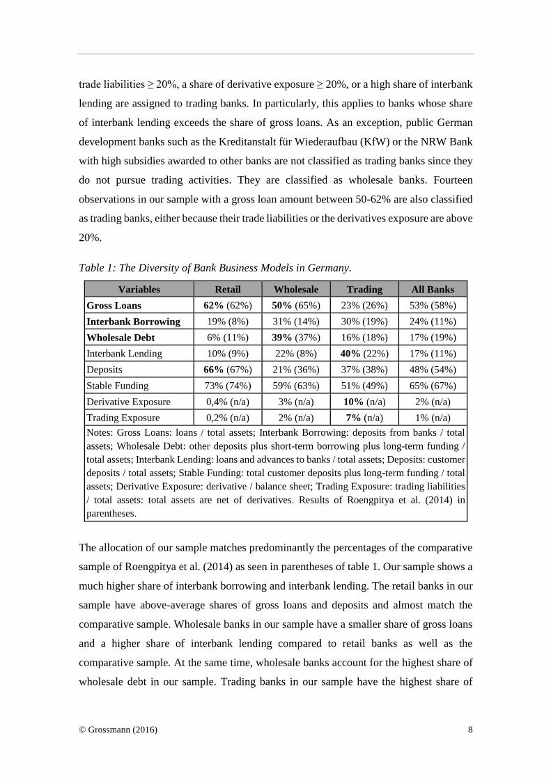
We adapt the three bank business models and use the above-mentioned key ratios

as well as five supportive ratios to allocate the banks in our sample as shown in table 1.

The supportive ratios are ‘Interbank Lending’, ‘Deposits’, ‘Stable Funding’, ‘Derivative

Exposure’, and ‘Trading Exposure’. At first, we look at banks with a high share of gross

loans above 50 percent on the balance sheet as well as the corresponding funding

structure. A retail bank is classified as a bank that depends largely on customer deposits

(≥ 50%). If the refinancing through interbank borrowing (i.e. bank deposits) and

wholesale debt (i.e. long-term liabilities, other deposits, and short-term bonds) exceed

customer deposits the bank is classified as a wholesale bank. In the second step, we look

at banks with a share of gross loans below 50 percent. Roengpitya et al. (2014) find that

trading banks hold about one-fifth of the balance sheet in interbank related assets and

liabilities. Therefore, banks whose trading activities are above-average with a share of


trade liabilities ≥ 20%, a share of derivative exposure ≥ 20%, or a high share of interbank

lending are assigned to trading banks. In particularly, this applies to banks whose share

of interbank lending exceeds the share of gross loans. As an exception, public German

development banks such as the Kreditanstalt für Wiederaufbau (KfW) or the NRW Bank

with high subsidies awarded to other banks are not classified as trading banks since they

do not pursue trading activities. They are classified as wholesale banks. Fourteen

observations in our sample with a gross loan amount between 50-62% are also classified

as trading banks, either because their trade liabilities or the derivatives exposure are above

20%.

Table 1: The Diversity of Bank Business Models in Germany.

Variables Retail Wholesale Trading All Banks

Gross Loans 62% (62%) 50% (65%) 23% (26%) 53% (58%)

Interbank Borrowing 19% (8%) 31% (14%) 30% (19%) 24% (11%)

Wholesale Debt 6% (11%) 39% (37%) 16% (18%) 17% (19%)

Interbank Lending 10% (9%) 22% (8%) 40% (22%) 17% (11%)

Deposits 66% (67%) 21% (36%) 37% (38%) 48% (54%)

Stable Funding 73% (74%) 59% (63%) 51% (49%) 65% (67%)

Derivative Exposure 0,4% (n/a) 3% (n/a) 10% (n/a) 2% (n/a)

Trading Exposure 0,2% (n/a) 2% (n/a) 7% (n/a) 1% (n/a)

Notes: Gross Loans: loans / total assets; Interbank Borrowing: deposits from banks / total

assets; Wholesale Debt: other deposits plus short-term borrowing plus long-term funding /

total assets; Interbank Lending: loans and advances to banks / total assets; Deposits: customer

deposits / total assets; Stable Funding: total customer deposits plus long-term funding / total

assets; Derivative Exposure: derivative / balance sheet; Trading Exposure: trading liabilities

/ total assets: total assets are net of derivatives. Results of Roengpitya et al. (2014) in

parentheses.

The allocation of our sample matches predominantly the percentages of the comparative

sample of Roengpitya et al. (2014) as seen in parentheses of table 1. Our sample shows a

much higher share of interbank borrowing and interbank lending. The retail banks in our

sample have above-average shares of gross loans and deposits and almost match the

comparative sample. Wholesale banks in our sample have a smaller share of gross loans

and a higher share of interbank lending compared to retail banks as well as the

comparative sample. At the same time, wholesale banks account for the highest share of

wholesale debt in our sample. Trading banks in our sample have the highest share of


interbank lending as well as derivative and trading exposure. For the comparison of the

results it has to be considered that not all data is available for the formulas ‘interbank

lending' and ‘interbank borrowing'. Hence, ‘reverse repurchase agreements and cash

collateral', which could be added to the counter of the formulas are not considered.

Altogether, our sample consists of 256 retail bank observations, 180 wholesale bank

observations, and 88 trading bank observations.

Methodical Framework

There is neither a generally accepted theory nor a widely shared model to develop a

leverage ratio requirement that will persuade policymakers, economists, and practitioners

at the same time. Exemplary, Hartmann-Wendels (2016) criticizes the leverage ratio as

unsuitable as a prudential measure and propagates that the leverage ratio will increase the

funding costs of banks. Therefore, we use a corporate finance methodology to test if the

irrelevance of capital structure applies to German banks and if the leverage ratio will raise

funding costs for different business models of banks.

One cornerstone of our model is the capital structure theory of Franco Modigliani

and Merton H. Miller. The M/M propositions state that the WACC of a company is

independent of the capital structure. That is, because the expected return on equity will

decrease once leverage is lowered. The cost for the higher share of equity will be offset

due to a reduced financial risk spread on equity. Lower leverage makes equity less risky.

At the same time, when the share of debt decreases the required interest rate of debt will

decrease as well, because the probability of default will be reduced. Overall, the WACC

stays unchanged (Modigliani and Miller, 1958). The M/M theorem assume perfect market

conditions, such as no transaction costs and identical financing costs for private and

corporate investors, but complicate the practical use. The M/M propositions will not be

used to increase bank's value, but will allow us to estimate the cost of capital for different

bank business models.

Our general methodology follows Miles et al. (2012) and the above-mentioned

studies, which have tested the M/M offset on listed banks in the UK, Europe, and the US.

For more details on the comparative studies see appendix I. In contrast, our focus is on a

sample of unlisted banks in Germany. Since the primary focus is on regulatory capital we

adapt the model of the WACC into the WAC(R)C for banks and focus on Tier 1 capital


and the expected return on Tier 1 capital only.5 The regulatory equity for a bank can be

divided into Tier 1 and Tier 2 capital. Tier 1 capital is referred to as going-concern capital

whereas Tier 2 capital is referred to as gone-concern capital. We use Tier 1 capital as

equity only since other components of bank’s equity such as convertible bonds (CoCos)

or Tier 2 capital can be seen as debt regarding accounting standards and tax law. Tier 1

capital consists of Common Equity Tier 1 (CET1) and Additional Tier 1 (AT1) capital

and is the sum of common shares, stock surplus, retained earnings, and accumulated other

comprehensive income as well as other disclosed reserves (BCBS, 2011). In addition,

Miles et al. (2012) refer to incomplete data regarding CET1 capital and use Tier 1 capital,

because they found a positive relationship between CET1 and Tier 1 capital. Furthermore,

the leverage ratio formula of Basel III focuses on Tier 1 capital because non-Tier 1 capital

components were seen less useful to absorb losses during the crisis (cf. BCBS, 2010).

The WAC(R)C is estimated as follows:

𝑊𝐴𝐶(𝑅)𝐶 = 𝑇𝑖𝑒𝑟1

𝑉 ∙ 𝑅𝑇𝑖𝑒𝑟1 +

𝐷

𝑉 ∙ 𝑅𝐷𝑒𝑏𝑡 ∙ (1 − 𝑡) (1)

where 𝑇𝑖𝑒𝑟1 is the amount of banks’ regulatory core capital, 𝑉 is the exposure measure

of a bank, 𝐷 the amount of debt, 𝑇𝑖𝑒𝑟1/𝑉 the equity ratio, 𝐷/𝑉 the debt ratio, and 𝑡 the

corporate tax rate. As for the capital cost rates, 𝑅𝑇𝑖𝑒𝑟1 is used as the expected return on

Tier 1 capital and 𝑅𝐷𝑒𝑏𝑡 as the interest rate on debt capital.

Since most German banks are not listed6 we use a proxy-model based on historical

returns instead of the capital-market-oriented CAPM, which is used by the comparative

studies, to determine the expected return on equity for investors.7 Thereby, actual realized

returns on equity might differ from previously calculated expected returns. Our approach

neglects the perfect market assumptions of the CAPM and estimates the cost of regulatory

equity under real market conditions with taxes. We do not rely on peer group betas or

other benchmarks, because they do not distinguish between bank business models. Our

model uses the historical net return on Tier 1 capital and leverage as the desired proxy.

5 For the distinction of bank’s capital for the WACC-Bank see Heidorn and Rupprecht (2009). 6 At the end of 2013 a total of 1,846 banks in Germany reported to the Deutsche Bundesbank (2015b).

Merely 19 of them were listed. Six listed banks are included in our sample. Listed banks are treated as

unlisted banks regarding the utilized variables. 7 Miles et al. (2012) suggest an alternative way to test the M/M effect by using expected earnings data.

Since expected earnings are commonly not published by banks, realized earnings over the stock price are

used by Miles et al. (2012) as a proxy for the expected return.


The statistical proxy-model does not calculate the risk premium, but the coefficients of

the model can reflect the risk preferences of investors (cf. Damodaran, 2013). Our idea

follows the approach of the BCBS (2010), who use the historical return on the risk-

weighted assets (RORWA) to set capital requirements for the risk-weighted approach. In

addition, book values rather than market-based values are used, because Tier 1 capital is

available as a book value only. The composition of bank’s assets is mostly based on

financial assets that are not subject to an ordinary depreciation. Therefore, the use of

bank’s book values is not directly comparable with the use of book values of non-financial

companies (Damodaran, 2002).

The Proxy-Model

For the expected return-proxy we use a panel regression approach. The regression models

are based on log regressions due to positively skewed distributions of the variables. The

regression is estimated as follows:

𝑙𝑛 (𝑅𝑇𝑖𝑒𝑟 1𝑖,𝑡) = 𝑎 + 𝑏 ∙ 𝑙𝑛(𝐿𝑒𝑣𝑒𝑟𝑎𝑔𝑒𝑖,𝑡) + 𝑐𝑖,𝑡 + 𝑧𝑡 + ɛ𝑖,𝑡 (2)

where 𝑖 = 1 to N is the individual bank and 𝑡 = 1 to T is the time index. We use 𝑎 as a

constant, 𝑏 as the coefficient of leverage and lagged leverage, and 𝑐 as a control variable

for additional explanatory bank effects. Further, 𝑧 is used for time specific effects (e.g.

time dummies) and use epsilon (ɛ) as the error term for the non-systematic part of the

regression model (cf. Wooldridge, 2002 and 2009).

The historical return on Tier 1 capital after taxes (𝑅𝑇𝑖𝑒𝑟 1) is used as the dependent

variable. We choose the net return since dividends on shares are paid to investors after

the company has paid corporate taxes. However, with the use of historical returns years

with financial loses are also included in the dataset. Negative returns occur in about 12.9

percent of the observations with a high share of about 70 percent during the financial

crisis between the years 2007 and 2011. Negative returns make it hard to interpret a year

of losses as a proxy for expected returns. First, it is a mathematical problem since negative

numbers cannot logarithmized. Secondly, investors would probably not invest if the bank

is expected to generate a loss. Therefore, we follow the suggestion provided by Cline

(2015) to swap negative returns for a minimum expected return of a five year Treasury


bond plus a risk spread of 100 basis points. We choose a five year period, because it can

be seen as the minimum maturity for capital to be accepted as equity.8 The return of a

German Treasury bond is measured from annual yields at the end of December. The data

is collected from the Deutsche Bundesbank (2015) and the yields are derived from the

term structure of interest rates on listed federal securities with annual coupon payments.

The risk spread used by Cline (2015) is based on the credit default swap spread for G-

SIB in the fourth quarter of 2012. The substitution of negative observations provides at

least a minimum expected return for investors of the proxy-model.

Leverage as the independent variable is measured as total assets divided by Tier 1

capital.9 We decide to use on-balance sheet exposure only, because off-balance sheet data

is not available for every bank in our sample. Because of changes in the definition of

Tier 1 capital during Basel I to III and the lack of adjusted Tier 1 capital figures during

the observed timeframe the ratios of leverage might not be entirely comparable to each

other. This should be considered when the results are interpreted. As for the explanatory

bank specific control variables we follow Miles et al. (2012) who use the return on assets

(ROA), a liquid asset ratio (LAR), and a loan loss reserve ratio (LLRR). The ROA is

measured as net income divided by total assets and reviews the profitability of the total

assets of a bank. The LAR is computed as liquid assets divided by total liabilities minus

Tier 1 equity and stands for the capability to sell assets without high losses. The LLRR is

calculated as the total loan loss reserves divided by total assets and checks for the

probability of potential future losses due to loan defaults. Furthermore, the size of a bank

(logarithm of total assets) as suggested by the ECB (2011) is used.

Statistics and Results

The descriptive statistics for the utilized dependent and independent variables, as

presented in appendix III, show that retail banks have an average leverage of 16.55, while

wholesale (28.71) and trading (35.49) banks account for a higher leverage. At the same

time, retail banks have the lowest realized return on Tier 1 capital with an average of

3.20% compared to wholesale (3.95%) and trading banks (4.95%). The descriptive results

for the sample seem to be comparable to the German banking market as a whole as a

8 See for example the criteria for inclusion in Additional Tier 1 capital (BCBS, 2011).

9 In contrast, the BCBS-leverage ratio is measured as Tier 1 capital divided by exposure measure.


study by Bain & Company shows. The analysis of 2,000 banks shows that the return on

Tier 1 capital after taxes has averaged 1.6% per year during the years 2011 and 2013.

(Sinn and Schmundt, 2014). The descriptive statistics indicate that bank’s leverage might

have an impact on the return on Tier 1 capital. The higher the leverage, the higher the

return. Four different regression models, one baseline model and three regression models

with additional control variables, are used to test for the empirical impact. We aim to find

a robust model to use the leverage coefficient of the proxy-model for the WAC(R)C.

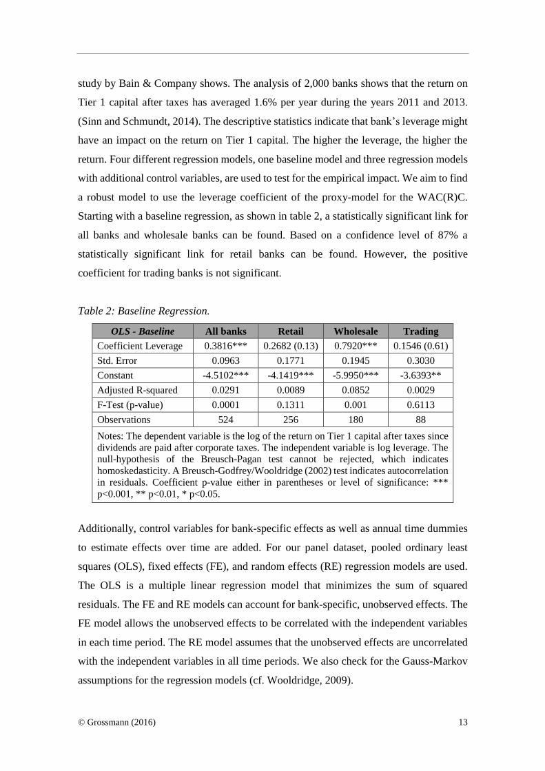
Starting with a baseline regression, as shown in table 2, a statistically significant link for

all banks and wholesale banks can be found. Based on a confidence level of 87% a

statistically significant link for retail banks can be found. However, the positive

coefficient for trading banks is not significant.

Table 2: Baseline Regression.

OLS - Baseline All banks Retail Wholesale Trading

Coefficient Leverage 0.3816*** 0.2682 (0.13) 0.7920*** 0.1546 (0.61)

Std. Error 0.0963 0.1771 0.1945 0.3030

Constant -4.5102*** -4.1419*** -5.9950*** -3.6393**

Adjusted R-squared 0.0291 0.0089 0.0852 0.0029

F-Test (p-value) 0.0001 0.1311 0.001 0.6113

Observations 524 256 180 88

Notes: The dependent variable is the log of the return on Tier 1 capital after taxes since

dividends are paid after corporate taxes. The independent variable is log leverage. The

null-hypothesis of the Breusch-Pagan test cannot be rejected, which indicates

homoskedasticity. A Breusch-Godfrey/Wooldridge (2002) test indicates autocorrelation

in residuals. Coefficient p-value either in parentheses or level of significance: ***

p<0.001, ** p<0.01, * p<0.05.

Additionally, control variables for bank-specific effects as well as annual time dummies

to estimate effects over time are added. For our panel dataset, pooled ordinary least

squares (OLS), fixed effects (FE), and random effects (RE) regression models are used.

The OLS is a multiple linear regression model that minimizes the sum of squared

residuals. The FE and RE models can account for bank-specific, unobserved effects. The

FE model allows the unobserved effects to be correlated with the independent variables

in each time period. The RE model assumes that the unobserved effects are uncorrelated

with the independent variables in all time periods. We also check for the Gauss-Markov

assumptions for the regression models (cf. Wooldridge, 2009).


All variables and logarithmized variables cannot reject the null-hypotheses of

the Jarque-Bera test for normal distribution. For all models, we can find significant

coefficients for leverage and ROA, but cannot find a positive link for the LLRR control

variable. For our OLS regressions, a positive link for the LAR and total assets can be

found. Statistically significant relationships for the LAR and total assets for the FE

models cannot be found. In addition, only a positive link for total assets with the RE

models is found. Overall, we decide to drop LLRR, LAR, and total assets as control

variables from all regressions, because they do not seem to have a constant statistically

significant impact on the return on Tier 1 capital for our German bank samples.

Table 3: Ordinary Least Squares (OLS) Regression.

OLS All banks Retail Wholesale Trading

Coefficient Leverage 0.7561*** 0.8829*** 0.9016*** -0.013 (0.96)

Std. Error 0.0953 0.1430 0.1850 0.3047

Constant -5.7614*** -6.7673*** -6.2448*** -3.0758*

Return on Assets 130.7990*** 171.8940*** 128.8235*** 76.4799**


F-Test (p-value) 0.0000 0.0000 0.0000 0.0001


Notes: The dependent variable is the log of the return on Tier 1 capital after taxes since

earnings are retained after corporate taxes. The independent variables are log leverage,

the return on assets, as well as year dummies. Annual time dummies are not shown.

The null hypotheses of the Breusch-Pagan test can be rejected, which indicates

heteroskedasticity. A Breusch-Godfrey/Wooldridge (2002) test indicates serial

correlation in residuals. Coefficient p-value either in parentheses or level of

significance: *** p<0.001, ** p<0.01, * p<0.05.

When using the remaining independent variables for the OLS regressions we find positive

relationships for the all bank, retail bank, and wholesale bank samples as shown in

table 3. However, a negative, albeit not significant link for trading banks is found. The

coefficients for the return on assets (ROA) indicate a strong positive link to the return on

Tier 1 capital. It seems reasonable that the return on total assets has a positive influence,

but the ROA cannot be attributed to regulatory capital as a whole. The positive correlation

of 0.50 – 0.67 between the return on Tier 1 and ROA for our sample indicates that other

components of bank’s equity or debt, regarding accounting standards and tax law, benefit

from the ROA as well. In addition, Clark et al. (2015) find a strong positive correlation


between the ROA and leverage and drop ROA from their regression models. For the

German bank sample, a negative correlation between ROA and leverage and decide to

keep ROA as a control variable is estimated.

For the within models in table 4, statistically significant relationships for all banks,

retail banks, and wholesale banks can be found. As for trading banks, we find a positive

link, but the model does not seem to be statistically significant. For the FE models, the

null-hypotheses for the Breusch-Godfrey/Wooldridge (2002) test that there is no serial

autocorrelation can be rejected, even when using one year lagged variables for leverage.

Table 4: Fixed Effects (FE) Regression.

FE All banks Retail Wholesale Trading

Coefficient Leverage 0.7887* 0.7620** 1.4403*** 0.1856 (0.79)

Std. Error 0.3316 0.2286 0.3534 0.7195

Return on Assets 83.9583*** 117.7354*** 99.656*** 40.214 (0.22)


F-Test (p-value) 0.0000 0.0000 0.000 0.1356


Notes: The dependent variable is log return on Tier 1 capital after taxes. The

independent variables are log leverage, the return on assets, and year dummies. Annual

time dummies are not shown. The results for the FE within models are computed by

one-way (individual) effects. Consistent standard errors based on Arellano (1987) are

used to address for heteroskedasticity and serial correlation. Coefficient p-value either

in parentheses or level of significance: *** p<0.001, ** p<0.01, * p<0.05.

Further, the null-hypotheses of the Breusch-Pagan test can be rejected, which indicates

heteroskedasticity for the FE and for the RE models as well. For that reason, robust

covariance matrix estimators by Arellano (1987) for the FE and RE models for our

unbalanced panel dataset are chosen. The Arellano estimator permits heteroskedasticity

and serial correlation.10

The last of the four regression models is the RE model. We test for the empirical

relationship of leverage on the return on Tier 1 capital and assume that unobserved effects

are uncorrelated with the independent variables. For the RE models in table 5, statistically

significant links for all banks, retail banks, and the wholesale bank sample are estimated.

10 We do not use robust standard errors by Driscoll and Kraay (1998), because our timeframe is shorter than

the recommended minimum timeframe of 20 to 25 years. Instead, the vcovHC function with the Arellano

estimator in ‘R’ as offered by Croissant and Millo (2008) is used.


As for the trading banks, a significant link based on the number of observations for our

sample cannot be found. We expect to find a positive and significant link between the

return on Tier 1 capital and leverage for trading banks once the number of observations

can be increased. Unfortunately, we are not able to increase the number of observations

(e.g. lengthening the timeframe) for German trading banks. We decide to neglect the

trading bank sample for the remainder of this paper. A serial correlation in residuals for

the RE models is not found as the null-hypotheses of the Breusch-Godfrey/Wooldridge

(2002) test cannot be rejected for all banks (p-value 0.1227), retail banks (p-value

0.1190), and wholesale banks (p-value 0.1806).

Table 5: Random Effects (RE) Regression.

RE All banks Retail Wholesale Trading

Coefficient Leverage 0.6891*** 0.8113*** 1.1938** -0.022 (0.95)

Std. Error 0.1799 0.1576 0.3592 0.3908

Constant -5.6628*** -6.6019*** -7.4776*** -3.1020*

Return on Assets 106.0138*** 159.9156*** 107.1911*** 64.5662**


F-Test (p-value) 0.0000 0.000 0.0000 0.0006


Notes: The dependent variable is the log of the return on Tier 1 capital after taxes. The

independent variables are log leverage, the return on assets, and annual time dummies.

Yearly time dummies are not shown. The results for the RE models are computed by

one-way (individual) effects. Consistent standard errors based on Arellano (1987) in

the plm.package of ‘R’ (Croissant and Millo, 2008) are used to address for

heteroskedasticity and serial correlation. Coefficient p-value either in parenthesis or

level of significance: *** p<0.001, ** p<0.01, * p<0.05.

After estimating three models with additional control variables we use statistical tests to

choose between the different regression models. First, the OLS and the FE models are

compared. We choose the FE models over the OLS models, because the null-hypotheses

for the F-test, which indicates no individual unobserved effects, can be rejected for all

banks (p-value 0.0000), retail banks (p-value 0.0000), and wholesale banks (p-value

0.0000). Secondly, the OLS and the RE regression models are compared. We use a

Lagrange Multiplier Test for panel models computed by Breusch-Pagan. If the null-

hypothesis can be rejected, the RE model is better. We find that the RE models seem to

be more appropriate than the OLS for all banks (p-value 0.000), retail banks (p-value


0.000), and wholesale banks (p-value 0.000). Thirdly, both the FE and RE models seem

to be consistent. Compared to the within models, the RE models have higher explanatory

values for the adjusted R-squared. To decide which model to use, we test for statistically

significant differences in the coefficient of the time-varying independent variables for the

FE and RE models by using a Hausman test (Wooldridge, 2009). The null-hypothesis

means that the differences in the coefficients are not significant and that unobserved

variables are not correlated with the independent variables. The Hausman test indicates

that the FE can be used for the all banks sample (p-value 0.0146). However, the null-

hypotheses cannot be rejected for the samples of retail banks (p-value 0.1833) as well as

wholesale banks (p-value = 1). Therefore, we decide to use the RE models. Overall we

choose the baseline regressions and the RE estimates as the proxy-model to calculate the

expected return of Tier 1 capital for the WAC(R)C.

Our results seem to be in line with the referred study of Miles et al. (2012), who

find a positive coefficient for leverage for the six largest UK banks of 0.6020 for a RE

log-model. Junge and Kugler (2012) observe Swiss banks and find a positive leverage

coefficient for the RE log-model of 0.7630. Furthermore, Clark et al. (2015) find a

positive coefficient of 0.9021 for a FE log model for the largest US banks between 2007

and 2012. In spite of the similarities, it is important to mention that the results are not

directly comparable due to the underlying assumptions, e.g. the use of control variables

and perfect capital markets (expected returns of the CAPM) vs. real market conditions

(actual realized returns of the proxy-model).

Calculating the WAC(R)C

Overall, the regression estimates for our proxy-model show that an increase of leverage

can be connected to a higher return on Tier 1 capital with measurable differences between

bank business models for our German sample. We use the coefficients of our regression

models to calculate 𝑅𝑇𝑖𝑒𝑟 1 for the above described formula of the WAC(R)C. The return

on Tier 1 capital can be calculated by inserting the constant and coefficient of leverage

into the proxy-model:

𝑒𝑥𝑝(𝑐𝑜𝑛𝑠𝑡𝑎𝑛𝑡 + 𝑐𝑜𝑒𝑓𝑓𝑖𝑐𝑖𝑒𝑛𝑡 ∙ 𝑙𝑛(𝐿𝑒𝑣𝑒𝑟𝑎𝑔𝑒)) = 𝑅𝑇𝑖𝑒𝑟 1 (3)


We use two exemplary illustrations for the calculation of the WAC(R)C and assume

identical equity ratios for the bank business models of 3% and 6%. For the debt part of

the WAC(R)C formula, we follow Junge and Kugler (2012) and use a constant rate of

debt of 1%. Using a constant debt rate is based on the comparative studies and enables a

comparison of the results. The debt rate seems to be in line with market conditions since

the end of 2011 when the yield of German treasury bonds with a maturity of five years

fell below 1% or since 2009 (and again 2011) when the ECB set the interest rate for main

refinancing operations at 1% (cf. Deutsche Bundesbank, 2015). The assumption of a

constant debt rate follows the idea that debt (e.g. savings deposits) can be seen as risk-

free due to deposit insurance and implicit state guarantees. Nonetheless, the probability

of default for debt can still be measured, but the value of risk-free debt is not correlated

with general market movements (Clark et al., 2015). If a nonconstant debt rate is assumed,

the probability of default could be measured by exploiting credit ratings for different bank

business models. However, both the German Savings Bank and Giro Association with

about 600 members as well as the German Cooperative Financial Network with about

1000 members have group ratings due to the ownership based liability system. As stated

above, the liability system does not allow us to differentiate between bank’s business

activities and the involved risks. Banks within one liability system might have different

rating grades if the ratings were based on the individual bank business model.

Additionally, G-SIB can have lower funding costs than non-systemically important banks

due to an expected state support (Ueda and Weder di Mauro, 2013). As for the corporate

tax rate a flat rate of 35% is used for our calculations.

Based on a 3% equity ratio and a debt rate of 1% the WAC(R)C for the all banks

sample would account for 0.756% (i.e. 3% ∙ 4.19% + 97% ∙ 1% ∙ (1-35%)). The

hypothetical doubling of equity for our illustrative calculations would increase the

WAC(R)C by 4.8 basis points to 0.804% (i.e. 6% ∙ 3.22% + 94% ∙ 1% ∙ (1-35%)). If we

assume that the M/M propositions would not hold at all investors would expect the same

return on equity regardless of leverage. Therefore, the WAC(R)C would increase by 10.6

basis points to 0.862% (i.e. 6% ∙ 4.19% + 94% ∙ 1% ∙ (1-35%)). If the M/M effect would

not be present the WAC(R)C would rise about 45% (4.8 bps./10.6 bps.). Conversely, the


M/M offset is about 55% for all banks in our sample.11 Table 6 shows the results of the

WAC(R)C calculations for the baseline models.

Table 6: Cost of Capital - Baseline.

Cost of Capital – Baseline All banks Retail Wholesale

Constant -4.5102 -4.1419 -5.9950

Coefficient Leverage 0.3816 0.2682 0.7920

𝑅𝑇𝑖𝑒𝑟 1 for 3% Equity Ratio 4.19% 4.07% 4.00%

WAC(R)C with 3% Equity Ratio 0.756% 0.753% 0.751%



Δ Impact on Cost of Capital 0.048% 0.061% -0.001%

Relative Impact 6.35% 8.10% -0.13%

M/M Offset 55% 40% 100%

Notes: The constants and coefficients are withdrawn from table 2. The return on

Tier 1 capital is based on the proxy-model. WAC(R)C is measured with a constant

interest rate for debt of 1% (risk-free debt) and a corporate tax rate of 35%. The

delta shows the impact of increased capital requirements on the overall funding

costs. The M/M offset describes to what part the WAC(R)C is independent of the

capital structure.

The assumption that higher equity ratios will reduce the risk of banks can be measured

by the required return on Tier 1 capital as it will drop from 4.07% to 3.38% for retail

banks and from 4.00% to 2.31% for wholesale banks. When comparing the relative

impacts of decreased leverage we find that the WAC(R)C of retail banks rises by 8.10%

compared to a drop of 0.13% for wholesale banks. If the interest rate for debt is changed

to 5% and neglect taxes (cf. Miles et al., 2012, ECB, 2011, and Clark et al., 2015) the

relative impact for retail banks would drop to -1.39% compared to -2.64% for wholesale

banks. If the M/M propositions completely hold the WAC(R)C would not change if

leverage decreases. However, the M/M offset of retail banks indicates a dependence of

the overall funding costs on bank’s capital structure. The irrelevance-effect for wholesale

banks seems to be stronger in the baseline model, because the WAC(R)C nearly stays the

same.

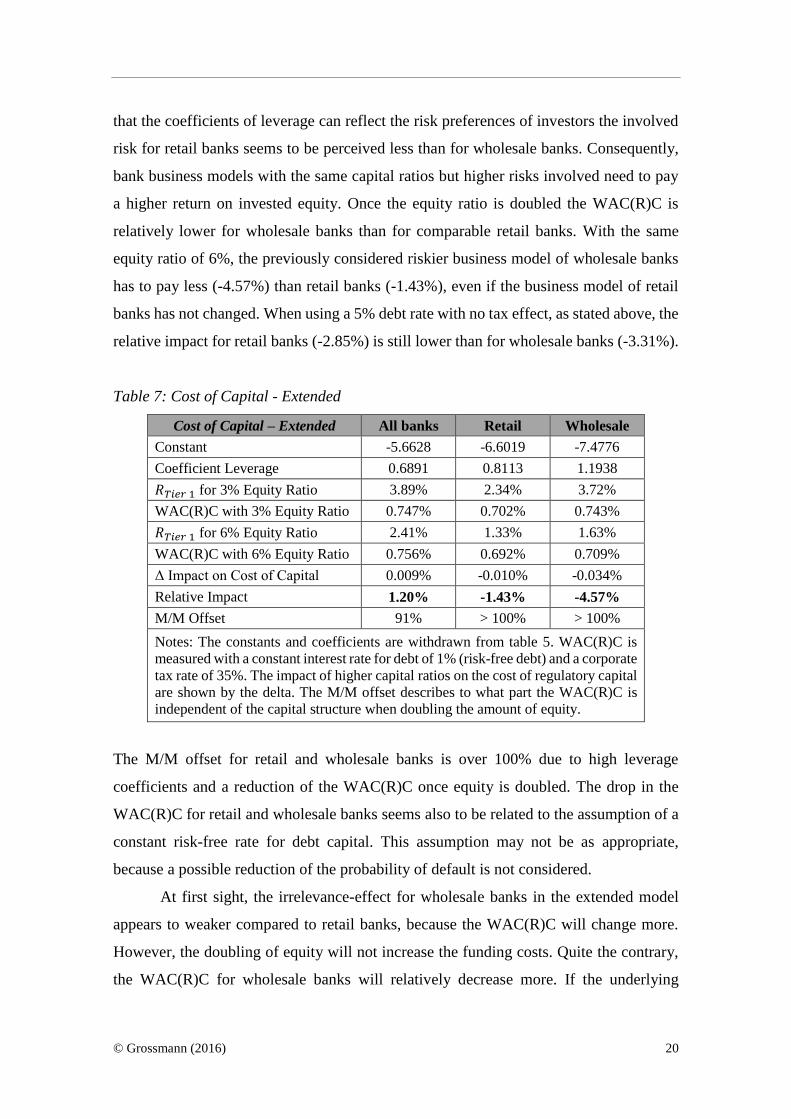
In the extended models with an equity ratio of 3% retail banks have lower overall

funding costs than comparable wholesale banks as shown in table 7. Given the assumption

11 An M/M offset of 100% describes a total independence of the cost of capital on the capital structure.


that the coefficients of leverage can reflect the risk preferences of investors the involved

risk for retail banks seems to be perceived less than for wholesale banks. Consequently,

bank business models with the same capital ratios but higher risks involved need to pay

a higher return on invested equity. Once the equity ratio is doubled the WAC(R)C is

relatively lower for wholesale banks than for comparable retail banks. With the same

equity ratio of 6%, the previously considered riskier business model of wholesale banks

has to pay less (-4.57%) than retail banks (-1.43%), even if the business model of retail

banks has not changed. When using a 5% debt rate with no tax effect, as stated above, the

relative impact for retail banks (-2.85%) is still lower than for wholesale banks (-3.31%).

Table 7: Cost of Capital - Extended

Cost of Capital – Extended All banks Retail Wholesale

Constant -5.6628 -6.6019 -7.4776

Coefficient Leverage 0.6891 0.8113 1.1938





Δ Impact on Cost of Capital 0.009% -0.010% -0.034%

Relative Impact 1.20% -1.43% -4.57%

M/M Offset 91% > 100% > 100%

Notes: The constants and coefficients are withdrawn from table 5. WAC(R)C is

measured with a constant interest rate for debt of 1% (risk-free debt) and a corporate

tax rate of 35%. The impact of higher capital ratios on the cost of regulatory capital

are shown by the delta. The M/M offset describes to what part the WAC(R)C is

independent of the capital structure when doubling the amount of equity.

The M/M offset for retail and wholesale banks is over 100% due to high leverage

coefficients and a reduction of the WAC(R)C once equity is doubled. The drop in the

WAC(R)C for retail and wholesale banks seems also to be related to the assumption of a

constant risk-free rate for debt capital. This assumption may not be as appropriate,

because a possible reduction of the probability of default is not considered.

At first sight, the irrelevance-effect for wholesale banks in the extended model

appears to weaker compared to retail banks, because the WAC(R)C will change more.

However, the doubling of equity will not increase the funding costs. Quite the contrary,

the WAC(R)C for wholesale banks will relatively decrease more. If the underlying


assumption is changed to a negative debt rate of 1% the WAC(R)C of wholesale banks

will change less (-1.05%) compared to retail banks (-5.23%). Again, the irrelevance-

effect applies differently to retail and wholesale bank business models.

Notes: The figures show the different impacts on the WAC(R)C for retail and wholesale banks

for an equity ratio of 3% and a potential doubling of equity to 6%. The irrelevance-effect is

stronger for wholesale banks in the baseline model. Due to the assumption of a constant risk-

free debt rate of 1% the WAC(R)C in the extended RE proxy-model will decrease if the equity

ratio is doubled. The WAC(R) for wholesale banks will relatively decrease more than for

comparable retail banks.

Figure 1: Unequal Impacts on the Cost of Regulatory Capital.

In both models (see figure 1) wholesale banks have an advantage of relatively lower

WAC(R)Cs compared to retail banks once equity requirements increase. The different

impacts on funding costs of overall 8.23% (8.10% vs. -0.13%) in the baseline models and

3.14% (-1.43% vs. -4.57%) in the extended models can lead to financial disadvantages.

We can conclude, that regardless of which regression model or assumption for the

WAC(R)C is used higher capital requirements can lead to unequal impacts on the cost of

regulatory capital in both the baseline and the extended calculations.

Conclusion

The Basel III leverage ratio is criticized that it could increase the cost of capital and lacks

to consider differences within the banking sector. Based on a proxy-model of historical

returns we find that funding costs of banks vary, but are partly independent of the capital

structure. The leverage ratio can lead to a slight increase of 6 basis points in the funding

costs of German banks, but will not force banks to assume higher risks. Higher capital

requirements are not free, but the amount seems to be acceptable to strengthen the

financial system. Furthermore, we find that higher capital ratios can have unequal impacts


on different bank business models. The paradoxical circumstance that previously

perceived riskier wholesale banks have to pay less than previously perceived less risky

business models once equity doubles can lead to financial disadvantages. The relative

impact on the funding costs seems in favor of wholesale banks, because the irrelevance-

effect is weaker for retail banks. The reason could be the funding structure. We find that

deposits are the most important source of debt refinancing for retail banks. However,

wholesale and trading banks use a broader mix of debt capital. A bank with a high share

of customer deposit funding might not be comparable to a low-deposit funded bank.

Further research could focus on the impact of deposit funding and the irrelevance of

capital structure.

The practical application of our paper is that economic and prudential goals can

be achieved simultaneously. This can mean for shareholders of different bank business

models: higher equity ratios do not increase the funding costs by a lot, but can reduce the

riskiness of banks. If the cost of capital can nearly stay the same, banks will have no need

to shift to higher-risk assets. And for regulators: identical capital requirements can have

diverse impacts on bank business models. The microprudential focus on the regulatory

cost of capital could complement the previous “rough indication” of the BCBS (2010)

to calibrate a leverage ratio requirement. If differences of bank business models will be

considered, a uniform leverage ratio may not lead to a more similar banking sector and

could compensate for possible competitive disadvantages. Consequently, the design of

unequal leverage ratios that consider individual risks regarding the size of a bank (cf.

Clark et al., 2015), the relevance to the financial system, and the bank business model is

desirable.


References

Admati, Anat R./DeMarzo, Peter/Hellwig, Martin/Pfleiderer, Paul (2013), Fallacies,

Irrelevant Facts, and Myths in the Discussion of Capital Regulation: Why Bank

Equity is Not Socially Expensive, Rock Center for Corporate Governance -

Working Paper Series No. 161, Stanford.

Arellano, Manuel (1987), Computing robust standard errors for within group estimators,

in: Oxford Bulletin of Economics and Statistics, 49, pp. 431-434.

Ayadi, Rym/De Groen, Willem Pieter (2014): Banking Business Models Monitor 2014

Europe, Centre for European Policy Studies and International Observatory on

Financial Services Cooperatives, Brussels.

Bankscope-Database, Bureau van Dijk Electronic Publishing (2015), Hanauer Landstraße

175-179, 60314 Frankfurt am Main, Germany.

Basel Committee on Banking Supervision (2010), Calibrating regulatory minimum

capital requirements and capital buffers: a top-down approach, Bank for

International Settlements, Switzerland.

Basel Committee on Banking Supervision (2011), Basel III: A global regulatory

framework for more resilient banks and banking systems, December 2010

(rev June 2011), Bank for International Settlements, Switzerland.

Basel Committee on Banking Supervision (2014), Basel III leverage ratio framework and

disclosure requirements, January 2014, Bank for International Settlements,

Switzerland.

Clark, Brian/Jones, Jonathan/Malmquist, David (2015), Leverage and the Weighted-

Average Cost of Capital for U.S. Banks, online available at:

http://papers.ssrn.com/sol3/papers.cfm?abstract_id=2491278 (18.10.2015).

Cline, William, R. (2015), Testing the Modigliani-Miller Theorem of Capital Structure

Irrelevance for Banks, Working Paper Series, Peterson Institute for International

Economics, Washington.

Croissant, Yves/Millo, Giovanni (2008), Panel Data Econometrics in R: The plm

Package, in: Journal of Statistical Software 27(2), online available at:

http://www.jstatsoft.org/v27/i02/. (25.09.2015).

Damodaran, Aswath (2002), Investment Valuation, Tool and Techniques for Determining

the Value of Any Asset, 2nd edition, New York.


Damodaran, Aswath (2013), Equity Risk Premiums (ERP): Determinants, Estimation

and Implications – The 2013 Edition (March 23, 2013), online available at:

http://ssrn.com/abstract=2238064 (06.02.2015).

Deutsche Bundesbank (2015), Time Series BBK01.WT3404 for a five year German

Treasury bond, online available at: http://www.bundesbank.de/Navigation/ DE/

Statistiken/Zeitreihen_Datenbanken/Makrooekonomische_Zeitreihen/its_details

_value_node.html?tsId=BBK01.WT3404&dateSelect=2013 (04.05.2015).

Deutsche Bundesbank (2015b), Banking statistics June 2015, Statistical Supplements to

the Monthly Report, Frankfurt am Main.

Deutsche Bundesbank (2015c), Structural developments in the German banking sector,

in: Deutsche Bundesbank, Monthly Report, April 2015, Vol. 67, No. 4, pp. 35-60,

Frankfurt am Main.

European Central Bank (ECB) (2011), Common Equity Capital, Banks‘ Riskiness and

Required Return on Equity, in: Financial Stability Report (December), pp. 125-

131, Frankfurt am Main.

Frenkel, Michael/Rudolf, Markus (2010), The implications of introducing an additional

regulatory constraint on banks’ business activities in the form of a leverage ratio,

online available at: https://www.bis.org/publ/bcbs165/rmafm.pdf (20.08.2015).

Hartmann-Wendels, Thomas (2016), The Leverage Ratio, design, supervisory objectives,

impact on bank’s business policy, online available at: http://www.die-deutsche-

kreditwirtschaft.de/uploads/media/110109_en_komplett_final.pdf (03.03.2016).

Heidorn, Thomas/Rupprecht, Stephan (2009), Einführung in das

Kapitalstrukturmanagement bei Banken, Frankfurt School – Working Paper

Series No. 121, Frankfurt an Main.

Hull, John C. (2015), Risk Management and Financial Institutions, Fourth edition,

New Jersey.

International Monetary Fund (IMF) (2014), Global Financial Stability Report - Risk

Taking, Liquidity, and Shadow Banking, Curbing Excess while Promoting

Growth, October 2014, Washington.

Junge, Georg/Kugler, Peter (2012), Quantifying the impact of higher capital requirements

on the Swiss economy, WWZ Discussion Paper 2012/13, online available at:

http://www.econbiz.de/themes/econbiz/images/icons/avail/pdf.png (14.08.2015).


Kiema, Illka/Jokivuolle, Esa (2013), Does a leverage ratio requirement increase bank

stability?, in: Journal of Banking and Finance, 39 (2014), pp. 240-254.

Miles, David/ Yang, Jing/Marcheggiano, Gilberto (2012), Optimal Bank Capital, in: The

Economic Journal, Vol. 123, pp. 1-37.

Miller, Merton H. (1995), Do the M & M propositions apply to banks?, in: Journal of

Banking and Finance, Vol. 19, pp. 483-489.

Modigliani, Franco/Miller, Merton H. (1958), The Cost of Capital, Corporation

Finance and the Theory of Investment, in: The American Economic Review,

Vol. 48, No. 3, June 1958, pp. 261-297.

Pfleiderer, Paul C. (2015), On the Relevancy of Modigliani and Miller to Banking: A

Parable and Some Observations (Revised), Stanford Graduate School of Business.

Roengpitya, Rungporn/Tarashev, Nikola/Tsatsaronis, Kostas (2014), Bank business

models, BIS Quarterly Review, December 2014, pp. 55-65, Switzerland.

Sinn, Walter/Schmundt, Wilhelm (2014), Deutschlands Banken 2014: Jäger des

verlorenen Schatzes, Bain & Company, Germany.

Toader, Oana (2013), Estimating the Impact of Higher Capital Requirements on the Cost

of Equity: An Empirical Study of European Banks, in: International Economics

and Economic Policy, No. Dec, 2014, online available at:

http://ssrn.com/abstract=2357472 (14.08.2015).

Ueda, Kenichi/Weder di Mauro, Beatrice (2013), Quantifying structural subsidy values

for systemically important financial institutions, in: Journal of Banking and

Finance, Vol. 37, pp. 3820-3842.

Wooldridge, Jeffrey, M. (2002), Econometric Analysis of Cross-Section and Panel Data,

MIT Press, USA.

Wooldridge, Jeffrey, M. (2009), Introductory Econometrics, A Modern Approach, fourth

international student edition, Canada.


Appendix I. Comparative studies.

Miles et al.

(2012)

ECB

(2011)

Junge and

Kugler (2012)

Toader

(2013)

Clark et al.

(2015)

Cline

(2015)

Location UK International

G-SIBs Swiss Europe USA USA

Sample 6 banks 54 banks 5 banks 85 banks 200 banks 51 banks

Timeframe 6/1997 – 6/2010 6/1995 – 6/2011 6/1999 – 6/2010 1997 – 2012 3/1996 – 12/2012 2001 – 2013

Data origin n/a Bloomberg Datastream,

FINMA Bankscope

Chicago FED,

CRSP

Bloomberg,

bank’s websites

Regression 𝛽 = 𝑋′𝑏 + (𝛼 + 𝜇)

𝛽 = 𝑎 + 𝑏 ∙ 𝐶𝑅 +

𝑋 + 𝑑 + 𝑢

log(𝛽) =

𝑎 + 𝑏 ∙ 𝑙𝑜𝑔(𝑙𝑟) +

𝜂 + 𝛿 + 휀

𝛽 = 𝛼 + 𝑋′𝐶𝑅 + 𝑢 𝛽 = 𝑏 + 𝑥 + 𝑧 + 𝜇 𝑁𝐼/𝐸 = 𝑎 + 𝑧 + 𝑑

Variables12

𝛽 – Equity beta

𝑋 – Lagged

leverage + year

dummies

𝑏 – Control var.

𝛼 – Bank specific

effect

𝜇 – Error term


𝑎 – Fixed effects

𝐶𝑅 – Lagged

capital ratio

𝑋 – Control var.

𝑑 – Time fixed

effects

𝑢 – Error term


𝑎 – Constant

𝑙𝑟 – Leverage

𝜂 – Bank specific

effect

𝛿 – Time specific

effect

휀 – Error term


𝐶𝑅 – Capital

ratio- RWA

𝑋 – Bank specific

control variable

and time dummy

𝑢 – Error term


𝑏 – Lagged

leverage

𝑥 – Bank-specific

variables

𝑧 – Year dummy

or macro. variable

𝜇 - Error term

𝑁𝐼/𝐸 – Net

income to equity

ratio

𝑎 – Constant

𝑧 – ratio of debt

to equity

𝑑 – dummy

variable

Control

Variables13

- LLRR

- LAR

- ROA

- ROA

- Size

- RWA

n/a

- LLRR

- LAR

- ROA + Size

- LLRR

- LAR

- ROA

n/a

12 Variables: Leverage = Total assets / Tier 1 capital; Capital ratio (CR) = Tier 1 capital / Total assets; Capital ratio-RWA = Tier 1 capital / RWA. 13 Control Variables: Loan loss reserve ratio (LLRR) = Total loan-loss reserves / Assets; Liquidity (asset) ratio (LAR) = (Cash/ deposits of depository institution +

Available-for-Sale securities) / (Total liabilities – equity); Return on assets (ROA) = Net income / Total assets; Size = logarithm of total assets.


Coefficient

OLS: 0.025***

RE: 0.025***

FE: 0.031***

No control var.:

-0.045***

With control var.:

-0.079***

n/a

OLS: -0.022***

RE: -0.0257***

FE: -0.0259***

FE Basic:

0.064***

FE Extended:

0.062***

OLS: 0.636***

RE: n/a

FE: 0.708

Coefficient

Log-Model

OLS: 0.602***

RE: 0.602***

FE: 0.692***

n/a

OLS: n/a

RE: 0.763**

FE: 0.554**

OLS: -0.251***

RE: -0.418***

FE: -0.426***

OLS: n/a

RE: n/a

FE: 0.902***

n/a

Observations n/a 652 – 1,372 n/a 721 10,577 579

R-squared 0.634 – 0.671 0.360 – 0.530 0.307 – 0.849 0.025 – 0.099 0.395 – 0.486 0.268

Specific

model

characteristics

Control variables

were dropped

because of no

significance

- Log-RWA

- Log-Total assets

(Size) n/a

- Log-CR-RWA

- Log-Total assets

(Size)

- ‘Expected’ ROE

- Pre/post crisis

- Size 200 bn. $

- Leverage ≤

66.67

- Actual returns

- Swap negative

returns

M/M Offset 45% – 90% 41% – 73% 36% – 55% 42% 41% – 100% 60%

Level of significance: ***p<0.01, **p<0.05, *p<0.1


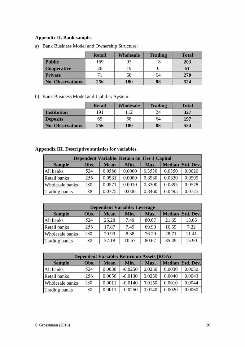
Appendix II. Bank sample.

a) Bank Business Model and Ownership Structure:

Retail Wholesale Trading Total

Public 159 93 18 203

Cooperative 26 19 6 51

Private 71 68 64 270

No. Observations 256 180 88 524

b) Bank Business Model and Liability System:

Retail Wholesale Trading Total

Institution 191 112 24 327

Deposits 65 68 64 197

No. Observations 256 180 88 524

Appendix III. Descriptive statistics for variables.

Dependent Variable: Return on Tier 1 Capital

Sample Obs. Mean Min. Max. Median Std. Dev.

All banks 524 0.0586 0.0000 0.3530 0.0350 0.0620

Retail banks 256 0.0531 0.0000 0.3530 0.0320 0.0599

Wholesale banks 180 0.0571 0.0010 0.3300 0.0395 0.0578

Trading banks 88 0.0775 0.000 0.3460 0.0495 0.0725

Dependent Variable: Leverage


All banks 524 25.28 7.49 80.67 21.65 13.05

Retail banks 256 17.87 7.49 69.90 16.55 7.22

Wholesale banks 180 29.99 8.38 76.29 28.71 11.41

Trading banks 88 37.18 10.57 80.67 35.49 15.90

Dependent Variable: Return on Assets (ROA)


All banks 524 0.0030 -0.0250 0.0250 0.0030 0.0050

Retail banks 256 0.0050 -0.0130 0.0250 0.0040 0.0043

Wholesale banks 180 0.0011 -0.0140 0.0150 0.0010 0.0044

Trading banks 88 0.0011 -0.0250 0.0140 0.0020 0.0060

LEVERAGE RATIO: ONE SIZE DOES NOT FIT ALL ANNUAL MEETINGS... · LEVERAGE RATIO: ONE SIZE DOES NOT...

Documents

Transcript of LEVERAGE RATIO: ONE SIZE DOES NOT FIT ALL ANNUAL MEETINGS... · LEVERAGE RATIO: ONE SIZE DOES NOT...