An (S, s) Model of Capital Structure:

Theory and Evidence∗

Arthur Korteweg

Graduate School of Business

Stanford University

Ilya A. Strebulaev

Graduate School of Business

Stanford University

and NBER

August 17, 2012

Abstract

We develop a general (S, s) model of capital structure that allows us to in-

vestigate the relationship between target leverage, refinancing thresholds, and

firm characteristics in a dynamic environment. We show that traditional em-

pirical methods used in capital structure may give misleading results, if firms

exhibit non-linear behavior. Empirical results reveal the substantial differences

between traditional and (S, s)-based analyses, which suggests the need for a

deeper exploration of (S, s) models. The findings should apply to most ar-

eas of corporate finance research and call for caution while using reduced-form

empirical tests.

∗We thank Nick Bloom, Murray Frank, Mike Harrison, Han Hong, Michael Roberts, Ken Sin-

gleton, and participants of seminars at Arizona State University, HEC Lausanne, London School

of Economics, Maastricht University, Penn State University, Stanford Graduate School of Business,

University of Toulouse, as well as at the 2010 Minnesota Corporate Finance Conference, 2011 UBC

Winter Finance Conference, and 2012 American Finance Association meetings for their helpful dis-

cussions and comments.

Understanding the cross-sectional properties of leverage ratios rests at the heart

of empirical capital structure research and constitutes perhaps the most important

link between empirical analysis and capital structure theory. From classical early

studies by Taggart (1977), Marsh (1982), and Titman and Wessels (1988) to the

most recent contributions in the field,1 linear regressions have been the workhorse for

exploring cross-sectional and time-series variation in capital structure. The estimated

determinants of corporate financial decisions are typically used to compare the results

with empirical predictions of various theories, or used in further investigation, such

as the analysis of target leverage or capital structure mean reversion. This empirical

search for “target” leverage ratios is well-grounded in many static models of corporate

financial structure, which contain a long list of comparative statics predictions.

Simple data analysis suggests, however, that linear models do not provide an

accurate representation of the data generating process. For example, cross-sectional

distributions of leverage are asymmetric and leverage is adjusted infrequently and

nonlinearly in time series. In this paper, we start by showing that in many realistic

situations, relying on traditional empirical methodology results in substantial biases

about both a “simple” variable such as the cross-sectional target leverage ratio and

the relationship between leverage and its covariates. We then develop an alternative,

non-structural model that more accurately captures the salient features of the data.

Our contribution is two-fold. First, we provide new evidence and insight into capital

structure determination. Second, and more important, we present a new theoretically

motivated and robust empirical method that is based on simple economic intuition

and that can account for non-linear dynamics. Furthermore, as will become clear,

the pitfalls that are associated with assuming a linear process (e.g., a dynamic model

without adjustment costs or a mean-reverting leverage model) and our suggested

1For a comprehensive overview of classical empirical studies of capital structure, see Harris and

Raviv (1991). An incomplete list of important recent work includes Hovakimian, Opler, and Titman

(2001), Baker and Wurgler (2002), Fama and French (2002), Korajczyk and Levy (2003), Flannery

and Rangan (2006), Kayhan and Titman (2007), Lemmon, Roberts, and Zender (2008), Byoun

(2008), Huang and Ritter (2009), Harford, Klasa and Walcott (2009), Chang and Dasgupta (2009),

Frank and Goyal (2009), and Denis and McKeon (2010).

2

remedy are not confined to capital structure, which we have chosen as the vehicle

to illustrate our findings, but also can be directly applied to other areas of financial

economics, such as corporate investment and cash policies.

To understand the crux of the matter, note that the standard econometric method-

ology estimates conditional expected leverage ratios, E(L|X), where L is the (vari-

ously defined) leverage ratio and X is the set of firm- or industry-specific determi-

nants, using method-of-moments estimators, either OLS or GMM. The mean/fitted

leverage ratios are often interpreted in a structural manner to provide insights about

capital structure policies. Unfortunately, in a dynamic world, the traditional method

works only if firms readjust to the target instantaneously, which is a highly unlikely

scenario, according to both accumulated empirical evidence and simple economic in-

tuition. For example, we show that in a dynamic world in which firms do not readjust

continuously to the target leverage ratio (e.g., if they face a small fixed transaction

cost of refinancing), The dynamic behavior of individual firms follows a highly non-

linear process and produces cross-sectional distributions of leverage that are highly

asymmetric around the target leverage ratio, leading to non-trivial biases in method-

of-moments estimators. Thus, the estimate of E(L|X) is not the target leverage

ratio. Therefore, it is not clear how to interpret the results obtained from traditional

empirical methods in relation to firms’ active capital structure decisions.

The main contribution of this paper is to develop a new general approach to

study corporate financial decisions that would lead to better inference in a dynamic

world. Specifically, we build and implement a dynamic (S, s) model of capital struc-

ture. The (S, s) model, developed originally by Arrow, Harris, and Marshak (1951),

has been used actively in economics to study cash balances, inventories, corporate

investment decisions, and consumer demand (e.g., Miller and Orr (1966), Caballero

(1993), Eberly (1994), Attanasio (2000), Caplin and Leahy (2006; 2010)). Our basic

economic assumption in developing an (S, s) model for capital structure research is

that firms follow a target leverage policy but, because of imperfections, deviate from

their target. The existence of the target leverage ratio, L∗, assumes the existence of a

trade-off between the benefits and costs of debt financing, which leads to an interior

3

solution at the firm level. In turn, there must exist a certain loss function that speci-

fies the cost that the firm incurs if it deviates from its preferred target leverage ratio.

This loss function in principle can be very generic. In capital structure, the losses

would include (but are not limited to) lost tax shields, costs of financial distress such

as debt overhang and asset substitution, and increased agency costs.

In developing an (S, s) model for capital structure, we take into account many

additional salient features of the leverage data generating process that are absent in

other (S, s) applications. For example, the refinancing thresholds may vary over time,

and have error components that are not perfectly correlated between the upper and

the lower threshold. Also, many leverage measures are naturally bounded (e.g., the

market leverage ratio is less than or equal to 1).

We then apply the (S, s) model to quarterly Compustat data on non-financial

firms between 1984 and 2009 and compare the results with an OLS approach. In

many instances, the estimates of target leverage coefficients have the same sign as

the OLS coefficients but are of a very different magnitude. In many important cases,

though, even the qualitative implications are different. For example, the OLS ap-

proach reliably produces a negative relation between leverage and profitability. The

(S, s) model instead produces a positive relation between profitability and target

leverage.

Using the (S, s) approach also enables us to study, for the first time, the deter-

minants of refinancing triggers. We find that firms allow leverage to float in a wide

range around the target, suggesting that either adjustment costs are high or the loss

of value from being away from the target capital structure is low, at least for moderate

leverage ratios. The thresholds vary predictably with firm characteristics such as the

market-to-book ratio, asset tangibility and research and development expenses. In

some cases, the thresholds are more sensitive to the covariates than the target capital

structure, and we find that some of the traditional regression results are driven by

the refinancing thresholds rather than the target leverage. For example, the negative

relation between earnings volatility and leverage in standard OLS regressions turns

out to be driven by the upper refinancing threshold, whereas the target leverage is

4

unrelated to earnings volatility.

In addition, (S, s) models are consistent with many contingent claims capital struc-

ture models that have been actively developed in recent years.2 At the same time,

an important advantage of the (S, s) approach is that we do not need to specify the

functional form of frictions or the stochastic process of the underlying model’s state

variables. The methodology does not rely on the exact economic mechanism, and

various conjectures can be comfortably nested together. This benefit comes at a cost,

though, because our results are harder to interpret in terms of underlying fundamen-

tals. It is thus important to stress that this methodology complements rather than

substitutes for the model-based structural estimation that has been gaining atten-

tion recently (e.g. Hennessy and Whited (2005, 2007), Nikolov and Whited (2011)).

For example, with the assumption that firms behave according to a particular dy-

namic model, a structural estimation should produce a much better estimate if the

assumptions prove correct.

To summarize, our overall contribution is two-fold. Empirical capital structure

researchers working on non-structural estimations should recognize that in the esti-

mation of the target leverage that firms adopt at refinancing, or its determinants,

cross-sectional or panel OLS regressions (or their more sophisticated moment-based

cousins) with the leverage ratio as the dependent variable may give misleading results,

if firms exhibit non-linear behavior. Our second contribution stems from the alter-

native empirical method that we develop to study determinants of active financial

decisions by corporations.

Ours is not the first paper to identify various problems with traditional empirical

methods in capital structure. Strebulaev (2007) shows that popular regressions of

profitability on leverage cannot be interpreted as finding the true relation between

profitability and target leverage. Morellec et al. (2012) also note that the conditional

mean of leverage does not correspond to the target leverage in a contingent claims

2Some examples include Fischer, Heinkel, and Zechner (1989), Goldstein, Ju, and Leland (2001),

Strebulaev (2007), Bhamra, Kuehn, and Strebulaev (2010a;2010b), and Morellec, Nikolov, and

Schuerhoff (2012).

5

model of the firm. They instead use a simulated maximum likelihood approach to

estimate their model. This method exploits the entire conditional distribution of

leverage but is sensitive to modeling and distributional assumptions. In contrast, our

approach is robust to a wide range of models.

We wish to stress that, although we present our results only in application to cap-

ital structure, its implications are likely applicable to a much broader range of topics

for which the dynamic behavior of agents (firms, consumers, investors, governments)

leads to an asymmetric cross-sectional distribution of the variables of interest, such

as cash flow and payout policies, corporate investment policy with fixed adjustment

costs, or a government economic policy that intervenes only when a certain indicator

(e.g., unemployment) rises above a threshold. Average investment or average unem-

ployment measures are likely meaningless in these settings and alternative measures

akin to the ones we propose herein need to be developed accordingly. Another ex-

ample is workforce adjustments in the presence of hiring and firing costs (e.g., Pfann

and Palm, 1993)

The remainder of the paper is structured as follows. Section I discusses the mean-

based analysis of leverage and introduces a general (S, s) model of capital structure.

Section II develops an empirical (S, s) model of capital structure. In Section III,

we describe the data sample, and in Section IV, we describe our empirical results.

Section V concludes.

I Mean-Based Analysis of Leverage

In this section, we show that mean-based analysis introduces potential biases into a

dynamic environment where leverage does not adjust instantaneously to its target.

We start by discussing implicit assumptions behind traditional capital structure re-

gressions. Then, we develop a general (S, s) model that enables us to analyze the

properties of the average leverage ratio in dynamics.

6

A Capital structure regressions

To study the empirical relationship between leverage and firm characteristics, the

standard approach has been to estimate the linear regression:

L = X ′β + ε, (1)

where the unit of observation is, say, a firm-year, and X includes a constant. One in-

terpretation of this regression is purely descriptive, capturing basic correlations in the

data. Some researchers, however, grant this regression a “structural” interpretation,

viewing the model as a way to estimate target leverage, L∗:3

L∗ = X ′β. (2)

Researchers are interested in target leverage because it is an outcome of active finan-

cial decisions by the firm. Although these two equations bear a close resemblance,

they are not equivalent. The regression model (1) includes an error term, such that

we could write L = L∗ + ε. The nature of the error term is critical, because it deter-

mines whether OLS estimates are consistent estimates of β in (2) and thus whether

they can be interpreted in a structural manner. The conditions for ε are the standard

OLS identification assumptions (assuming X includes a constant):

E(ε) = 0, (3)

Cov(X, ε) = 0. (4)

In a static setting, or a dynamic setting with no deviations from target leverage,

firms’ leverage ratio is always at L∗, and the error term represents unobserved (to

the econometrician) cross-sectional factors that affect L∗. The empirical issues in

this case are well-known: The coefficient estimates may be biased if X is jointly

determined with leverage or if there are omitted variables that are correlated with

X . In addition, in a dynamic world, deviations of leverage from its target may be

correlated with X (Strebulaev (2007)). All of these complications are violations of

the second identification assumption.

3E.g., Fama and French (2002) and Korajczyk and Levy (2003).

7

We show that the identification assumptions are violated even if the covariates in

X are exogenous, there are no omitted variables, and deviations from L∗ are purely

random. Consider as an example a generic dynamic model with fixed adjustment

costs, where leverage follows a stochastic process until it hits an upper (lower) rebal-

ancing point Lu (Ld), at which the firm rebalances to L∗. This is an example of an

eponymous (S, s) model. With leverage following an arithmetic Brownian motion,

the distribution of leverage for this simple model is as shown in Figure 1. The graph

shows that the mean of leverage is not equal to L∗. In other words, E(ε|X) 6= 0,

which implies a violation of the first identification assumption (X only includes a

constant here, but this statement holds more generally). Moreover, the mean of ε

varies with firm characteristics X , which determine L∗ and the location of the thresh-

olds. Therefore, not only is the intercept in regression (1) inconsistent, but so are the

estimates of β. We show that this result holds quite generally.

In a dynamic world with adjustment costs, even instrumental variables (IVs)

or differences-in-difference regressions from natural experiments may not correctly

identify the impact of an exogenous shock on target capital structure. First, the

shock may not be large enough for firms to adjust, which is essentially a “weak

instruments” problem. Second, and more worrisome, if the object of interest is the

change in a firm’s target leverage, then the magnitude may be biased for the same

reasons as the β estimates are biased in (1), namely, the difference between the true

target L∗ and the mean of leverage is not fixed. In other words, the change in the

conditional mean of leverage is not the same as the change in L∗. If the natural

experiment also changes Ld, Lu, or the shape of the loss function, even the sign of

the IV or differences-in-differences regressions may be wrong, such as would occur if

a natural experiment were to change the fixed cost of adjustment.

We explore the generality of this example by studying the relationship between

mean leverage and target leverage in a dynamic context. In Section II, we build a

new class of empirical models based on the (S, s) paradigm.

8

B Cross-sectional distribution of leverage in dynamics

B.1 General (S, s) model setup

To develop a general (S, s) model of capital structure, we assume the existence of

a certain loss function that specifies the cost the firm incurs if it deviates from its

preferred target leverage ratio. This loss function in principle can be very generic. In

capital structure, the losses include (but are not limited to) lost tax shields, costs of

financial distress such as debt overhang and asset substitution, and increased agency

costs.4

The optimality of an (S, s) policy also implies the existence of an adjustment

cost function that makes continuous small adjustments suboptimal. An important

type of cost function that we consider here involves fixed adjustment costs.5 Leary

and Roberts (2005) consider other examples of the adjustment cost function, such as

convex and fixed plus linear; it is important to generalize our results to cover these

cases as well.

In continuous time, assume that leverage, in the absence of a company’s active

intervention, follows an Ito process:

dLt = µ(Lt)dt+ σ(Lt)dBt, (5)

where µ(L) is the instantaneous growth parameter, σ(L) is the instantaneous volatility

parameter, and B is the standard Brownian motion defined on a filtered probability

space under the physical measure P. Unless it may lead to ambiguity, we drop the t

subscript in our subsequent discussion. Furthermore, we assume that the parameters,

µ and σ, can depend on time only through the effect of leverage, implying the existence

of its stationary distribution. Although this is a reasonable assumption, in principle,

4Note that for our purposes, the optimality of “target” leverage and other parameters of interest

is immaterial. The distinction between various definitions of leverage is not important either and in

this section we do not specify the “leverage ratio” any further.5The result that fixed costs lead to an impulse control problem, where the variable of interest

follows an exogenously specified stochastic process in the inaction region and is reset when it hits

lower and upper triggers is well-known in stochastic optimal control literature. See Harrison, Sellke,

and Taylor (1982) for an early development and Stokey (2009) for a textbook treatment.

9

various extensions that include non-stationary cases can be considered.

The (S, s) policy means that leverage follows (5) in the inaction region, which is

the region of leverage ratios between the upper and lower threshold. With a convex

loss function, when leverage hits the lower threshold, denoted by Ld, or the upper

threshold, denoted by Lu, Ld ≤ L∗ ≤ Lu ≤ 1, the firm refinances, and the process is

reset at L∗.6 Then, as long as L ∈ (Ld, Lu), the firm remains in the inaction region

at date t. The leverage process is illustrated in Figure 2.

Proposition 1 derives the stationary distribution of leverage, f(L), in the general

case:

Proposition 1 The stationary distribution of leverage. Let leverage follow

(5), for L ∈ (Ld, Lu). If leverage hits either Ld or Lu, it is reset to L∗, where

Ld ≤ L∗ ≤ Lu. Define X as:

X ≡

Γ(Ld, L∗) Γ(L∗, Lu)∫ L∗

Ld z(L)Γ(Ld, L)dL −∫ Lu

L∗z(L)Γ(L, Lu)dL

, (6)

where:

Γ(a, b) ≡

∫ b

a

γ(L)dy, (7)

γ(L) ≡ exp

[−

∫ L 2µ(L)

σ2(L)dy

], (8)

z(L) ≡1

γ(L)σ2(L). (9)

Then a unique stationary distribution of leverage, f(L), exists if and only if the

determinant of the matrix X is non-zero. Then, f(L) is given by:

f(L) =

z(L)

[A1

∫ Lγ(y)dy +B1

], for Ld ≤ L ≤ L∗,

z(L)[A2

∫ Lγ(y)dy +B2

], for L∗ ≤ L ≤ Lu,

(10)

where A1, A2, B1, and B2 are constants determined by the boundary conditions:

6To provide some intuition behind Lu, in many capital structure models, the upper refinancing

threshold implies that the firm enters financial distress and defaults. This is a special case of our

framework when Lu = 1. As in many models, we assume that once the firm reaches the upper

threshold, it readjusts back to the same target level.

10

1. f(Ld) = 0,

2. f(Lu) = 0,

3. limL↓L∗ f(L) = limL↑L∗ f(L),

4.∫ Lu

Ld f(L)dL = 1.

Figure 1 shows an example of the stationary leverage distribution for the case where

L follows an arithmetic Brownian motion. The figure illustrates the basic and yet

fundamental result of this section: Leverage distributions are asymmetric around L∗.

The implications of such asymmetry are profound. First, the mean of the asymmetric

distribution is not equal to L∗, barring knife-edge type solutions. As we show later,

for an arithmetic Brownian motion, L∗ is always the mode of distribution, rather

than its mean. In other words, for that particular example, it is not clear that the

average leverage ratio is informative about the target leverage ratio. Second, and most

important, applying mean-based capital structure regressions to data taken from such

a distribution will likely result in substantial bias. These two results constitute an

intuitive property of dynamic leverage distributions. Although no further results can

be derived about the general solution for the mean and the shape of the stationary

leverage distribution, the following three examples illustrate that this result is very

general.

B.2 Examples

Example 1: Arithmetic Brownian motion. If leverage follows the arithmetic

Brownian motion process, that is, if µ(L) = µ and σ(L) = σ, the next proposition

shows the stark result that L∗ is almost never the mean of the distribution.

Proposition 2 Target leverage for the ABM case. If leverage follows (5)

in the inaction region, and µ(Lt) = µ and σ(Lt) = σ, then L∗ = m(L), where m(L) is

the mode of the leverage distribution, for any values of µ, σ, Ld , L∗, and Lu subject

to Ld < L∗ < Lu.

11

For an asymmetric distribution the mean is almost never equal to the target

leverage (which equals the mode of the distribution), and only in rare cases is the

distribution symmetric (e.g., when L∗ − Ld = Lu − L∗ and µ = 0).

Example 2: Geometric Brownian motion. Consider the case in which lever-

age follows the geometric Brownian motion process between refinancings, such that

µ(L) = µL and σ(L) = σL. The next lemma derives the stationary cross-sectional

distribution of leverage in this case:

Lemma 1 Stationary distribution of leverage for the GBM case. If

leverage follows (5) in the inaction region L ∈ (Ld, Lu), µ(Lt) = µL, σ(Lt) = σL, the

leverage restarts at L∗ at both triggers Ld and Lu, and µ 6= 12σ2, then the stationary

distribution of target leverage L∗ is:7

fGBM (L) =

[Ld

L−(

Ld

L

)−k+2]/C1, for Ld < L ≤ L∗,

[Lu

L−(Lu

L

)−k+2]/C2, for L∗ < L < Lu,

(11)

for k 6= 1, where k ≡ 2µ/σ2, and

C1 ≡ Ld

[− log

(Ld

L∗

)+ log

(Lu

L∗

)·1− (L

d

L∗)−k+1

1− (Lu

L∗)−k+1

], (12)

C2 ≡ Lu

[− log

(Ld

L∗

)·1− (L

u

L∗)−k+1

1 − (Ld

L∗)−k+1

+ log

(Lu

L∗

)]. (13)

Figure 3 shows two typical examples of this distribution. In both examples, the

distribution is again, as expected, asymmetric. In the first example, target leverage

equals the mode, as in the example above, whereas in another case it is higher than

the mode but also unlikely to be equal to the mean. As the next proposition shows,

these two examples exhaust the possibilities.

Proposition 3 Target leverage for the GBM case. If leverage follows (5)

in the inaction region, µ(Lt) = µL, and σ(Lt) = σL, then the target leverage L∗

is equal to the mode m(L) of distribution fGBM (L) if either k ≥ 2 or k < 2 and

m(L) <(

12−k

) 1k−1 Ld. Otherwise, it is greater than or equal to the mode.

7The special and uninteresting case, µ = 1

2σ2, is given in Appendix A.

12

The proposition shows that the target leverage ratio L∗ is the mode if either µ > σ2 or

m(L) <(

12−k

) 1k−1 Ld. The latter condition is satisfied whenever µ or Ld are sufficiently

large, and it is likely to hold for many reasonable scenarios.

For this case, the proposition implies that because the cross-sectional stationary

distribution is asymmetric, we again should expect the mean leverage ratio to dif-

fer generally from L∗, barring some knife-edge type solutions, and any mean-based

empirical analysis of covariates therefore should be biased.

Example 3: A dynamic model of capital structure In this example, we explore

a standard contingent-claims trade-off model of optimal dynamic capital structure.

The model set-up follows previous work such as that by Fischer, Heinkel, and Zechner

(1989), Goldstein, Ju, and Leland (2001), and Strebulaev (2007). A major distinction

from the previous examples is that neither the leverage process nor the (S, s) thresh-

olds are primitive variables; rather, they are outcomes of optimal decision-making by

firms that face a trade-off between the tax benefits of debt and the dead-weight losses

of default. The primitive variable is a pre-tax cash flow or EBIT, Xt, that follows a

geometric Brownian motion process under the actual probability measure:

dXt = µPXtdt+ σXtdBt, (14)

where µP is the instantaneous growth parameter of cash flows under the actual prob-

ability measure and σ is the instantaneous cash flow growth volatility.8 At the same

time, all the optimal decisions are made under the risk-neutral measure Q. The

derivation of the optimal leverage ratio is standard, and the solution of the model

is given in Appendix B. For our purposes, it is sufficient to note that in this model,

XR is the upper refinancing threshold (equivalent to Ld), and XB is the bankruptcy

threshold (equivalent to Lu = 1). The first-order homogeneity property ensures sure

that to derive the stationary distribution of leverage, it is sufficient to assume that

whenever X reaches any of the thresholds, it is reset at its original value, X0.

8Note that thus far we have used µ and σ for the drift and volatility of leverage. Here, the same

parameters refer to the drift and volatility of earnings, and P emphasizes that probabilities are taken

under the actual measure.

13

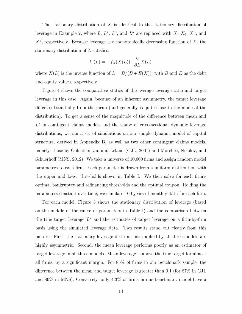
The stationary distribution of X is identical to the stationary distribution of

leverage in Example 2, where L, L∗, Ld, and Lu are replaced with X , X0, Xu, and

Xd, respectively. Because leverage is a monotonically decreasing function of X , the

stationary distribution of L satisfies:

fL(L) = −fX(X(L)) ·∂

∂LX(L),

where X(L) is the inverse function of L = B/(B+E(X)), with B and E as the debt

and equity values, respectively.

Figure 4 shows the comparative statics of the average leverage ratio and target

leverage in this case. Again, because of an inherent asymmetry, the target leverage

differs substantially from the mean (and generally is quite close to the mode of the

distribution). To get a sense of the magnitude of the difference between mean and

L∗ in contingent claims models and the shape of cross-sectional dynamic leverage

distributions, we ran a set of simulations on our simple dynamic model of capital

structure, derived in Appendix B, as well as two other contingent claims models,

namely, those by Goldstein, Ju, and Leland (GJL, 2001) and Morellec, Nikolov, and

Schuerhoff (MNS, 2012). We take a universe of 10,000 firms and assign random model

parameters to each firm. Each parameter is drawn from a uniform distribution with

the upper and lower thresholds shown in Table I. We then solve for each firm’s

optimal bankruptcy and refinancing thresholds and the optimal coupon. Holding the

parameters constant over time, we simulate 100 years of monthly data for each firm.

For each model, Figure 5 shows the stationary distribution of leverage (based

on the middle of the range of parameters in Table I) and the comparison between

the true target leverage L∗ and the estimates of target leverage on a firm-by-firm

basis using the simulated leverage data. Two results stand out clearly from this

picture. First, the stationary leverage distributions implied by all three models are

highly asymmetric. Second, the mean leverage performs poorly as an estimator of

target leverage in all three models. Mean leverage is above the true target for almost

all firms, by a significant margin. For 85% of firms in our benchmark sample, the

difference between the mean and target leverage is greater than 0.1 (for 87% in GJL

and 80% in MNS). Conversely, only 4.3% of firms in our benchmark model have a

14

mean leverage within 0.05 of the true target (4.4% in GJL and 7.6% in MNS) and

only 0.6% have a mean within 0.01 of the target (0.7% in GJL and 1.1% in MNS).

Our evidence thus strongly suggests that the mean leverage ratio is not informative

about target leverage and that mean-based analysis in this case may lead to non-

trivial biases. We proceed to develop a general framework that takes these issues into

account.

II Empirical (S, s) Model of Capital Structure

We estimate the benchmark capital structure (S, s) model, where for firm i at time t:

L∗it = X ′

itβ + u∗it, (15)

Luit = L∗

it + exp(X ′itθ

u + uuit), (16)

Ldit = L∗

it − exp(X ′itθ

d + udit). (17)

Equation (15) models target leverage, L∗it, and appears analogous to the traditional

regression model (1), which is ubiquitous in extant literature. However, as we discuss

next, the identification and interpretation of this equation are quite different in the

(S, s) model. The exponential terms in (16) and (17) represent the gap between

the upper refinancing threshold, Luit, and target leverage, and the gap between the

lower threshold, Ldit, and target, respectively. The use of the exponential function

guarantees that the target leverage is located between the two thresholds. The vector

of explanatory variables, Xit, is assumed to be the same for the target and the two

thresholds.

The distribution of the error terms is assumed to be jointly Gaussian:

u∗it

uuit

udit

∼ N

0

0

0

,

(σ∗)2 ρ∗uσ∗σu ρ∗dσ∗σd

· (σu)2 0

· ·(σd)2

. (18)

The errors are i.i.d. across firms and time and uncorrelated with Xit. The likelihood

function for this model is derived in Appendix C.

15

Our empirical model is based on other applications of (S, s) models. For example,

Attanasio (2000) uses a similar structure to estimate an (S, s) model for consumers’

automobile purchases as a function of time-invariant household characteristics, while

imposing a common error term on the upper and lower thresholds. Applying this

methodology to capital structure, however, introduces a number of novel features.

First, we need to allow for time-varying covariates, which results in time-variation in

the thresholds. Second, because the upper and lower thresholds on capital structure

are driven by fundamentally different considerations, we allow for separate error terms

in the upper and lower adjustment thresholds. Third, there are natural bounds on

the values that leverage may take, which may differ by measure. For example, market

leverage is naturally bounded above by 1, and leverage measures gross of cash are

bounded below at 0. It is important to recognize these bounds in the estimation.

The parameters of target leverage, β, are identified from the first observation of

leverage following a refinancing event, when the firm returns to L∗. For example, if

L∗ is the mode of the stationary leverage distribution, as in our examples in Section

I.B, then β can be interpreted as determining the conditional mode of the leverage

distribution as a linear function of X . The error term, u∗, captures explanatory

variables that are omitted from X . In addition, in practice leverage is reported only

at discrete intervals, and so it typically is not observed by empiricists immediately

upon refinancing. Leverage may have moved away from the true L∗ in the period

between refinancing and observation, introducing an additional observation error.

Furthermore, L∗ may have changed over this period. The estimate of σ∗ captures

both sources of error.

We can learn about the upper and lower thresholds from the periods of inaction,

in which firms do not refinance. For the firms that do not refinance in the current

period, leverage is between the thresholds, Ldit < Lit < Lu

it. This condition yields a

lower bound on Luit and an upper bound on Ld

it. With discrete time, leverage may

still move beyond its current value before the actual refinancing event takes place

(even if that happens in the next period), and without further assumptions we can

only identify a lower bound on Luit and an upper bound on Ld

it. We estimate the

16

parameters, θu and θd, that characterize these bounds. In the period before levering

down, the observed leverage ratio is the best estimate of the lower bound on Luit.

Similarly, the leverage in the period before levering up is the best estimate of the

upper bound on Ldit. With a high frequency of observations, the estimated bounds on

Lu and Ld will be close to the true refinancing thresholds. For statistical efficiency,

we use all observations of leverage to identify the parameters of these bounds, not

just the observations in the period before a refinancing. In the robustness section, we

explore an alternative estimation procedure that identifies the thresholds exactly, and

show that the empirical results are similar. Note that if we are in a static world or

a dynamic world without adjustment costs, our model would not converge, because

the coefficients in θu and θd that load on the intercept in X would tend to negative

infinity.9

The correlations between Lu and L∗, and between Ld and L∗ can be identified.

In the inaction region, we can learn about Lu (and hence uu) if leverage is above the

target (as partly determined by the realization of u∗). This reveals information about

the correlation between these two error terms. The same argument applies to ud and

u∗. However, the correlation between udt and uu

t in (18) is not identified, because in

no-refinancing periods we learn about either Luit or L

dit, not both simultaneously. In

the benchmark case, we assume this correlation to be zero.

An (S, s) model is essentially a reduced-form approach that relies on the generic

economic structure of the problem. It thus complements a more structural approach

to studying corporate financial decisions (e.g., Hennessy and Whited (2005; 2007)),

which may imply the same dynamic strategy. One advantage of estimating an (S, s)

model is its reliance on fewer assumptions about deep structural parameters that are

needed to estimate the dynamic behavior of firms. In particular, we do not make

any specific assumptions about the nature or functional form of tax benefits, costs of

financial distress, or agency costs. We also make no assumptions about the nature

9Note that our model is more informative than simply identifying the refinancing thresholds

from quantile regressions of leverage on the covariates (or the extremes of a firm’s leverage ratios),

as doing so would ignore the actual refinancing decisions.

17

of the driving stochastic process, whereas dynamic contingent claims models rely on

particular assumptions (e.g., a geometric Brownian motion for EBIT, an AR(1) pro-

cess for productivity). For example, our empirical model makes no assumptions about

the presence of jumps, whereas Kane, Marcus, and McDonald (1985) show that the

implications of jumps in the stochastic process are of first-order importance. In this

sense, the strengths of the (S, s) empirical method also helps pinpoint its weaknesses.

Although the approach is more general than a given model, it does not provide the

rich economic content underlying the mechanisms at work, as specific models do so

well, nor can it, of course, replace the need for a better understanding of the factors

that drive corporate decisions. Thus, a structural model and an (S, s) model should

be viewed as closely connected approaches that lead to the same ultimate goal.

III Data

To assemble the main sample, we start with quarterly data from Compustat between

1984 (the year quarterly equity issuance and repurchase data first became available)

and 2009. We exclude utilities (SIC codes 4900–4999) and financial firms (SIC codes

6000–6999) to avoid companies whose financial policies are largely driven by govern-

ment regulation. We also exclude companies with less than $10m in book assets, in

year 2000 dollars. We use leverage measures commonly employed in prior literature,

which we define as follows:

• Market leverage: book debt (the sum of short-term debt (DLCQ) and long-term

debt (DLTTQ)), divided by the sum of book debt and the market value of equity

(the product of shares outstanding (CSHOQ) and price per share (PRCCQ)).

• Net market leverage: book debt net of cash (CHEQ), divided by the sum of

book debt and the market value of equity.

• Book leverage: book debt divided by book assets (ATQ).

• Net book leverage: book debt net of cash divided by book assets.

The explanatory variables we employ are standard and are defined as follows:

18

• PROF : Profitability, measured as EBITDA (OIBDPQ) divided by book assets.

• MB : Market-to-book ratio, defined as the sum of the market value of equity

and book debt divided by book assets.

• PPE : Property, plant, and equipment (PPENTQ) divided by book assets.

• DEPR : Depreciation (DPQ) divided by book assets.

• RD : R&D expense (XRDQ) divided by book assets.

• RDdum : An indicator variable that equals 1, if the firm had a non-zero R&D

expense in the past quarter, and 0 otherwise.

• LN(TA): Natural log of book assets.

• VOL : Volatility of quarterly profitability over the past 10 years.

To minimize the influence of outliers, we trim net market and book leverage at

−1, as well as profitability, depreciation, R&D, and earnings volatility at the 99th

percentile; furthermore, we trim profitability at the 1st percentile and the market-to-

book ratio at 10.

Because an (S, s) model is inherently a model of dynamic capital structure, we

restrict the sample further to exclude firms with fewer than eight quarters of consec-

utive data. The final sample is an unbalanced panel of 5,252 firms spanning 160,305

firm-quarters. Table II reports summary statistics, and Figure 6 depicts histograms

for our leverage measures. Requiring at least two years of data inevitably introduces a

survivorship bias. Yet, compared with the full sample, there is no material difference

in leverage, though in our sample firms are slightly larger and more profitable, and

more firms have non-zero R&D expenditures (results not reported).

We define refinancing in a manner consistent with prior studies (e.g., Hovakimian,

Opler, and Titman (2001), Korajczyk and Levy (2003), Hovakimian (2004), Leary and

Roberts (2005), and Frank and Goyal (2009)). A firm is classified to have increased its

leverage in a given quarter if net debt issuance (debt issuance (DLTISY) minus debt

repurchases (DLTRY)) minus net equity issuance (equity issuance (SSTKY) minus

19

repurchases (PRSTKCY)) over the quarter is greater than 5% of the beginning-of-

quarter book value of assets.10 Conversely, if net equity issuance minus net debt

issuance is greater than 5% of book assets, the firm is designated to have reduced

its leverage. This definition of refinancing captures not only public but also private

debt issuance, the most prevalent form of debt financing (e.g., Houston and James

(1996), Bradley and Roberts (2004)). The 5% threshold is chosen to capture financ-

ing decisions that are intended to change capital structure, and it excludes most

“mechanical” issuance and repurchases, such as equity issuance due to the planned

exercise of executive stock options. As Leary and Roberts (2005) note, even though

this measurement may result in some misclassifications (such as the calling of con-

vertible debt or the transfer of equity accounts from subsidiaries to parents), the 5%

classification scheme produces results similar to using new debt and equity issuance

data from SDC (see also Hovakimian et al. (2001), Korajczyk and Levy (2003)).

Panel C of Table II reports summary statistics for refinancing activity. Firms

increase their leverage in 8.1% of the observed firm-quarters, and the median firm

increases leverage twice during the sample. When they increase leverage, firms issue

net debt in excess of net equity of 16% of book assets on average (median 10%).

Leverage decreases occur in 5.6% of the firm-quarters. The median firm reduces

leverage once and issues net equity in excess of net debt of 16% on average (median

9%). The distribution of refinancings is skewed: 15.9% of firms do not refinance in

the sample period, 15.0% refinance only once, and 10.3% of firms undergo 10 or more

refinancings. However, these numbers may overstate the number of true refinancings,

because some leverage rebalancings span more than one quarter. In the robustness

section, we show that our results are robust to grouping consecutive refinancing events

together.

10Compustat reports debt and equity issuance and repurchase variables on a cumulative basis

throughout the fiscal year, so for each variable we first obtain its net contribution for a given

quarter.

20

IV Empirical Analysis of the (S, s) Model

In this section, we discuss the results of the empirical analysis of the (S, s) model

of leverage. We first concentrate on target leverage, then turn to the results on the

refinancing thresholds. Finally, we explore the robustness of these results.

A Target leverage

Table III reports the parameter estimates of the (S, s) model, where we choose net

market leverage (i.e, leverage net of cash) as our benchmark proxy, as well as the

coefficients of a standard OLS regression of leverage on the covariates. Although we

concentrate first on the results for target leverage and their comparisons with those

derived from the OLS approach, it is important to stress that one of the critical

differences between the (S, s) and OLS modeling approaches is that the latter allows

the firm to adjust only leverage in response to changing covariates, whereas the former

provides the firm with two additional levels of control, namely, adjustments to the

upper and lower refinancing thresholds. Thus, the OLS approach, if taken as a

structural model, corresponds to a static world, in which adjustment costs are zero

(and thus, firms are always at the optimum). Any explanation in differences between

the results on target leverage should thus emphasize the additional flexibility of the

(S, s) approach.

The β coefficients in Table III show that target leverage is statistically significantly

higher for larger, more profitable firms with lower market-to-book ratios, higher tan-

gible assets, lower depreciation, and zero research and development outlays. Although

these coefficients have the same sign as the OLS estimates in most cases, the implied

economically meaningful magnitudes are vastly different. The most striking result,

though, involves the profitability coefficient. In standard OLS regressions, profitabil-

ity reliably has a strong negative relationship to leverage, consistent with prior studies

(see, e.g., Fama and French (2002)). In contrast, the (S, s) model yields a positive

relation between target leverage and profitability. The coefficient is statistically sig-

nificant at the 1% level and, as robustness tests show, is consistent across various

21

measures of leverage, although its economic significance is rather low, as Figure 7

indicates. Overall, the positive loading on profitability is consistent with a dynamic

trade-off model with adjustment costs. In that model, positive (negative) shocks

to profitability mechanically lower (increase) leverage, driving the negative OLS co-

efficient, even though the target leverage ratio is positively related to profitability

(Strebulaev (2007)).

To gain insight into the economic significance of the β estimates, in Figure 7 we

plot comparative statics of fitted target leverage, L∗ (marked with an “o”), along

with the OLS fitted values (marked with an “x”). For example, the top-left plot

shows target leverage for the three values of profitability at the 20th, 50th, and 80th

percentiles of the sample data, leaving all the other covariates at their sample median

values. The corresponding numerical values are in Table IV. The fitted target leverage

from the (S, s) model in Figure 7 is larger than the OLS point estimate across all the

covariates. The difference is economically large: The median firm’s target leverage is

0.23, compared with the OLS point estimate of 0.19. This difference suggests that the

underleverage result, widely documented in prior literature, may be less severe than

previously thought. As firms grow, the presence of adjustment costs induces them

to optimally allow leverage to drift down, resulting in lower leverage on average,

compared with their target leverage upon refinancing.

The magnitude and sign of the differences between the β and OLS coefficients

are driven by multiple factors. First, the drift and volatility of the leverage process

between refinancings (e.g., Equation (5)) may vary with the covariates. Table V

shows the coefficient estimates of regressions of firm-level leverage drift and volatility

on covariates, where drift is measured across non-refinancing periods. Most covariates

are statistically significantly related to the drift of leverage (the first column of the

table). For example, highly profitable firms have a faster growing market value of

equity, so their market leverage tends to drift down faster than that of less profitable

firms. Keeping the refinancing thresholds constant, this tendency shifts a greater mass

of the leverage distribution towards the lower values, decreasing the mean relative

to the target leverage. Coefficients on R&D and earnings volatility reveal the same

22

pattern (but not firm size). By the same token, the drift of leverage is higher for firms

with higher market-to-book ratios, tangible assets, depreciation, and R&D expenses.

For all of these covariates, apart from PPE and the R&D dummy, the OLS coefficients

in Table III are indeed higher than the corresponding values of β.

The volatility of the leverage process, absent refinancings, may also vary with the

covariates. The second column in Table V shows that most covariates are strongly

related to the volatility of the leverage process. All else being equal, a lower volatility

of the leverage process implies that the density of leverage has more mass concentrated

around the target leverage ratio, leading the OLS estimates to approach the β values.

For example, firms with a higher market-to-book ratio tend to have lower leverage

volatility. Figure 7 shows that the OLS fitted leverage is closer to the target leverage

when MB is high. The results for all covariates are consistent with this phenomenon,

except for profitability, depreciation, and R&D.

The second factor underlying the large differences between the β and OLS coef-

ficients is that these coefficients may be affected by the location of the refinancing

thresholds. If the thresholds vary systematically with the covariates, the conditional

mean of leverage, and thus the OLS estimates, may be pulled in the direction of

the threshold (in Figure 1, we see how the distribution, and thus the mean, of the

leverage distribution shifts if the thresholds shift). For example, the coefficient on

earnings volatility for target leverage in Table III is virtually zero, whereas the OLS

coefficient is −0.831. At the same time, the upper refinancing threshold loading on

earnings volatility is −1.202, and the lower threshold loading is virtually zero. Be-

cause the upper refinancing threshold is closer to target leverage for higher levels

of earnings volatility, the mass of the leverage distribution shifts towards the lower

leverage ratios, and therefore conditional mean leverage is pulled down relative to

target leverage. This mechanism results in a lower coefficient on earnings volatility

in OLS regressions relative to the corresponding β coefficient.

An important conclusion that can be made from these considerations is that it is

difficult to interpret the OLS fitted leverage ratios in a structural manner, because

they represent a simultaneous combination of forces related to the leverage diffusion

23

process, the target leverage, and the refinancing thresholds.

B Refinancing thresholds

The (S, s) approach enables us to introduce direct estimates of the refinancing bound-

aries into the capital structure literature and explore their dependence on covariates,

as well as their empirical relation to target leverage estimates. Table IV reveals that

the inaction region between the two refinancing thresholds is large: Firms allow their

leverage ratios to vary between the lower threshold of around −0.41 and an upper

threshold around 0.75.11 Although the magnitude of the gap is driven to a significant

extent by our use of a measure of the net of cash leverage, it still is notably large

for gross of cash measures. Unreported, for (gross) market leverage measure, the

corresponding lower (upper) thresholds are approximately 0.04 (0.57).

The width of the inaction region may be driven by either high costs of adjustment

or a low loss of value for being away from target leverage (these are not mutually

exclusive explanations). In particular, the large negative lower threshold indicates

that firms are not overly concerned with running large cash balances. This result is

consistent with Korteweg (2010), who finds that the present value of the net benefits

to leverage is quite flat for a large range of leverage ratios around the target. Korteweg

also documents that the size of issuance and repurchase transaction costs alone are

not enough to explain the deviations from the target observed in the data. Other

costs of adjustment, not captured by pure transaction costs, may include asymmetric

information costs of selling undervalued securities and management time spent raising

capital rather than running the firm (which may be especially high for distressed

firms).

The size of the inaction region may appear surprising, considering that the me-

dian firm appears to refinance once a year, as documented in Table II. However, the

distribution of refinancings is skewed, with 16% of firms choosing not to refinance

11Recall that the “upper” threshold is a leverage-reducing trigger, at which firms opt to refinance

when leverage is too high, whereas the “lower” threshold is a leverage-increasing trigger, at which

firms opt to refinance when leverage is too low.

24

at all over the sample period, and another 15% refinancing only once. Only a small

fraction of firms rebalance frequently. Moreover, single rebalancing events are often

implemented and reported over two consecutive quarters, likely overstating the true

number of refinancing actions, although the quantitative impact of “quarter stretch-

ing” is not immediately available to us. Finally, any deliberate temporary deviations

from (S, s) policies, such as those discussed by DeAngelo, DeAngelo, and Whited

(2011), may overstate the frequency of refinancings relative to the (S, s) model we

study here.

As Table IV shows, the upper and lower refinancing thresholds have different

sensitivities to the covariates. The upper refinancing threshold is decreasing in prof-

itability, whereas the lower threshold is not significantly related to it. Moreover, the

upper threshold is an order of magnitude more sensitive to profitability than the

target leverage. Overall, the results suggest that firms are most concerned about

their capital structure situation when leverage is high and the likelihood of financial

distress is non-trivial; they are less preoccupied with the decision to lever up (e.g.,

because of asymmetry in the value function, according to Korteweg (2010), who finds

that it is relatively flat for low but drops sharply for very high leverage ratios).

Table IV shows that several other variables, such as the market-to-book ratio,

tangibility, the R&D dummy, and size, are important drivers of both the upper and

lower refinancing thresholds. Many of these relationships are intuitive and in line with

well-known economic mechanisms. For example, the relationship between the market-

to-book ratio and the refinancing thresholds is consistent with the debt overhang

mechanism, where firms keep leverage in a lower range when they have substantial

growth opportunities. This mechanism also can explain the evidence regarding the

R&D dummy.

Tangible assets, as measured by PPE, are related strongly to both higher target

leverage and higher refinancing thresholds, implying that firms with a large proportion

of tangible assets find it advantageous to have high leverage. This result is consistent

with the lower costs of financial distress for such firms (e.g., due to lower fire-sale

costs). It is also consistent with a credit rationing story, in which firms with more

25

pledgeable assets are less constrained by creditors in taking on more debt. Both

thresholds and target leverage also increase with firm size, so large firms exhibit

significantly higher leverage ratios than small firms.

In a standard trade-off model, firms with higher earnings volatility have lower

leverage to avoid the negative consequences of financial distress, which occurs with

higher likelihood for more volatile firms (all else being equal). The negative coefficient

on earnings volatility in the OLS specification in Table III supports this explanation.

The (S, s) model estimates show, however, that the effect of earnings volatility works

mainly through the upper refinancing threshold: Firms with highly volatile earnings

reduce debt at lower leverage ratios than firms with stable earnings, whereas the

target leverage is not affected by earnings volatility. This mechanism affects leverage

parameters through financial distress, so it is not surprising that the lower refinancing

threshold is not related to earnings volatility. The same explanation can be applied

to research and development expenses.

Because the economic significance results in Table IV are based on comparative

statics, it is not clear how much variation in capital structure policies the model ac-

tually captures. To explore this question, Figure 8 shows histograms of the target

capital structure and the refinancing thresholds across 56 two-digit SIC code indus-

tries (excluding financials and any industries with fewer than 1,000 firm-quarter ob-

servations). For each industry, we calculate median industry characteristics and feed

them into the model using the parameter estimates of Table IV. The figure reveals

substantial variation not only in the target leverage ratio but also in the refinancing

thresholds across industries. The upper threshold is as low as 0.55 for plastics and

chemicals (SIC code 28), an industry characterized by high market-to-book and R&D

expenses, many intangible assets, and volatile earnings; it is as high as 0.88 for rail-

roads (SIC code 40), an industry with large firms mostly comprised of tangible assets,

few growth opportunities, and stable earnings. The lower threshold ranges from -0.60

for lab equipment (SIC code 38), an R&D-intensive industry with few tangible assets,

to -0.17 for railroads (SIC code 40).

26

C Robustness

As is true of any empirical study, it is important to verify whether our results are

driven by specific assumptions about variable construction or the estimation proce-

dure. As a first robustness check on our results, we run an alternative estimation

procedure that identifies the thresholds exactly, by assuming that the firm exceeded

the threshold in the period prior to refinancing. In this case, θu and θd have a dif-

ferent interpretation: They specify the exact threshold rather than a bound on the

thresholds. This exact identification comes at the cost of assuming that firms do

not immediately refinance after hitting the threshold, which is contrary to the intu-

ition of the (S, s) model (though it is possible to rationalize this behavior through,

for example, infrequent capital structure evaluation by management). It is, how-

ever, reassuring that the results under the two identification strategies turn out to be

quantitatively very similar.12

Second, we set the threshold for refinancing at 3% and 7% of book assets, instead

of the 5% used in the main results. The results are largely unaffected. The most

noteworthy change for the 7% threshold case is that the β-coefficient on DEPR

loses significance. For the 3% threshold case, the β-coefficient on PROF falls to

5% significance (but remains positive), the θu loading on LN(TA) flips sign from

negative and significant to positive and significant, and the θd loading on RD becomes

statistically significant at the 1% level (from a statistically insignificant loading in the

benchmark case).

For our third robustness test, we grouped consecutive refinancings together to

account for cases in which, for example, an equity issue and debt repurchase were

split across quarters. Most of our results are unchanged qualitatively, except for the

β-loading on DEPR, which becomes insignificant, and the θd-coefficients on R&D

and LN(TA) switch sign and become positive and significant at the 1% level.

Fourth, we included short-term debt changes in the definition of refinancing events.

Our main results use long-term debt issuance and repurchase only, since short-term

12Attanasio (2000) uses a similar identification strategy to the one we employ in our robustness

tests.

27

debt is often seasonal, and is missing in many cases. Including short-term debt reduces

the sample size in half, because of missing observations, but our results remain close

to the ones we reported in the previous subsections.

Fifth, we considered measures of leverage different from the benchmark net market

leverage that we used in the prior subsections. Using net book leverage gives very

similar results. The only notable differences are that the β-loading on DEPR and the

θu-loading on PROF become positive and significant. Using book leverage (gross of

cash) does not change our results qualitatively, unless we drop zero leverage firms, in

which case the β-coefficient on PROF turns negative. Using market leverage (gross

of cash) gives similar results to book leverage.

To summarize, we find that our main results are robust to using a different iden-

tification strategy, to using different measures of leverage, and to other variations on

data definitions.

V Conclusion

We propose and develop a general (S, s) model of capital structure, with which we

investigate the relationship between target leverage and its covariates in a dynamic

environment. Unlike traditional empirical capital structure methods, the (S, s) model

takes into account the non-linear dynamics of the leverage data generating process and

therefore can be more informative about multiple issues at the core of capital struc-

ture research, such as target leverage behavior. The empirical results show substantial

differences between the traditional mean-based and (S, s) models. In particular, the

target leverage in the (S,s) model is higher than the fitted value from the traditional

regressions, and the target leverage increases with profitability, in contrast with the

traditional regression results that suggest a negative relation between leverage and

profitability. We also offer several new results regarding the refinancing thresholds.

We show that firms allow leverage to float in a wide band around the target, and

we find that some of the standard OLS regression results are driven by the refinanc-

ing thresholds rather than the target leverage – such as the negative coefficients on

28

research and development outlays and earnings volatility.

Because this study is the first to estimate dynamic (S, s) models for capital struc-

ture, we have deliberately chosen a simple specification. Obviously, our (S, s) model

should be viewed as only the first step in building the next generation of dynamic

empirical models in capital structure and elsewhere in corporate finance. For ex-

ample, we assume the existence of only fixed costs of adjustment. In the presence

of both fixed and variable costs, the return points of target leverage differ between

upper and lower refinancing triggers. We also do not allow for predetermined financ-

ing events (e.g., when outstanding debt becomes due) or investment-driven financing.

The (S, s) method can be extended to include these and many other enriching features

in capital structure and, more generally, empirical corporate finance. We believe this

methodology is an important avenue for future research.

29

References

Arrow, Kenneth. J., T. Harris, and J. Marshak, 1951, Optimal inventory

policy, Econometrica 19, 250–272.

Attanasio, Orazio, P., 2000, Consumer durables and inertial behavior: Estima-

tion and aggregation of (S, s) rules for automobile purchases, Review of EconomicStudies 67, 667–696.

Baker, Malcolm, and Jeffrey Wurgler, 2002, Market timing and capital

structure, Journal of Finance 57, 1–32.

Bhamra, Harjoat S., Lars-Alexander Kuehn, and Ilya A. Strebulaev,

2010a, The aggregate dynamics of capital structure and macroeconomic risk, Review

of Financial Studies 23, 4187–4241.

Bhamra, Harjoat S., Lars-Alexander Kuehn, and Ilya A. Strebulaev,

2010b, The levered equity risk premium and credit spreads: A unified framework,Review of Financial Studies 23, 645–703.

Bradley, Michael, and Michael R. Roberts, 2004, The structure and pricing

of bond covenants, Working paper, University of Pennsylvania.

Byoun, Soku, 2008, How and when do firms adjust their capital structures towards

targets? Journal of Finance 63, 3069–3096.

Caballero, Ricardo, 1993, Durable goods: An explanation for their slow adjust-ment, Journal of Political Economy 101, 351–383.

Caplin, Andrew, and John Leahy, 2006, Equilibrium in a durables goods marketwith lumpy adjustment costs, Journal of Economic Theory 128, 187–213.

Caplin, Andrew, and John Leahy, 2010, Economic theory and the world of

practice: A celebration of the (S, s) model, Journal of Economic Perspectives 24,183–202.

Chang, Xin, and Sudipto Dasgupta, 2009, Target behavior and financing, Jour-

nal of Finance 64, 1767–1796.

DeAngelo, Harry, Linda DeAngelo, and Toni M. Whited, 2011, Capital

structure dynamics and transitory debt, Journal of Financial Economics 99, 235–261.

Denis, David J., and Stephen B. McKeon, 2010, Debt financing and finan-cial flexibility: Evidence from pro-active leverage increases, Working paper, Purdue

University.

Eberly, Janice C., 1994, Adjustment of consumers durable stocks: Evidence from

automobile purchases, Journal of Political Economy 102, 403–436.

Fama, Eugene F., and Kenneth R. French, 2002, Testing trade-off and peckingorder predictions about dividends and debt, Review of Financial Studies 15, 1–33.

Fischer, Edwin O., Robert Heinkel, and Josef Zechner, 1989, Optimaldynamic capital structure choice: Theory and tests, Journal of Finance 44, 19–40.

30

Flannery, Mark J., and Kasturi P. Rangan, 2006, Partial adjustment towardtarget capital structures, Journal of Financial Economics 79, 469–506.

Frank, Murray Z., and Vidhan K. Goyal, 2009, Capital structure decisions:

Which factors are reliably important? Financial Management 38, 1–37.

Goldstein, Robert, Nengjiu Ju, and Hayne E. Leland, 2001, An EBIT-

based model of dynamic capital structure, Journal of Business 74, 483–512.

Harford, Jarrad, Sandy Klasa, and Nathan Walcott, 2009, Do firms haveleverage targets? Evidence from acquisitions, Journal of Financial Economics 93,

1–14.

Harris, Milton, and Arthur Raviv, 1991, The theory of capital structure,Journal of Finance 46, 297–355.

Harrison, Michael J., T. L. Sellke, and A. J. Taylor, 1982, Impulse controlof Brownian motion, Mathematics of Operations Research, 8, 454–466.

Hennessy, Christopher A., and Toni M. Whited, 2005, Debt dynamics, Jour-

nal of Finance 60, 1129–1165.

Hennessy, Christopher A., and Toni M. Whited, 2007, How costly is external

financing? Evidence from a structural estimation, Journal of Finance 62, 1705–1745.

Houston, Joel, and Christopher James, 1996, Bank information monopoliesand the determinants of the mix of private and public debt claims, Journal of Finance

51, 1863–1889.

Hovakimian, Armen, 2004, The role of target leverage in security issues and re-

purchases, Journal of Business 77, 1041–1071.

Hovakimian, Armen, Tim Opler, and Sheridan Titman, 2001, Debt-equitychoice, Journal of Financial and Quantitative Analysis 36, 1–24.

Huang, Rongbing, and Jay Ritter, 2009, Testing theories of capital structure

and estimating the speed of adjustment, Journal of Financial and Quantitative Anal-ysis 44, 237–271.

Kane, Alex, Alan J. Marcus, and Robert L. McDonald, 1985, Debt policyand the rate of return premium to leverage, Journal of Financial and Quantitative

Analysis 20, 479–499.

Karlin, Samuel, and Howard M. Taylor, 1981, A second course in stochasticprocesses, Academic Press: New York.

Kayhan, Ayla, and Sheridan Titman, 2007, Firms’ histories and their capitalstructures, Journal of Financial Economics 83, 1–32.

Korajczyk, Robert A., and Amnon Levy, 2003, Capital structure choice:

Macroeconomic conditions and financial constraints, Journal of Financial Economics68, 75–109.

Korteweg, Arthur G., 2010, The net benefits to leverage, Journal of Finance 65,

2137–2170.

31

Leary, Mark T., and Michael R. Roberts, 2005, Do firms rebalance theircapital structure?, Journal of Finance 60, 2575–2619.

Lemmon, Michael L., Michael R. Roberts, and Jaime F. Zender, 2008,

Back to the beginning: Persistence and the cross-section of corporate capital struc-ture, Journal of Finance 63, 1575–1608.

Marsh, Paul, 1982, The choice between equity and debt: An empirical study,

Journal of Finance 37, 121–144.

Miller, Merton, and Daniel Orr, 1966, A model of demand for money by

firms, Quarterly Journal of Economics 80, 413–435.

Morellec, Erwan, Boris Nikolov, and Norman Schurhoff, 2012, Corpo-rate governance and capital structure dynamics, Journal of Finance 67, 803–848.

Nikolov, Boris, and Toni M. Whited, 2011, Agency conflicts and cash: Esti-mates from a structural model, Working paper, University of Rochester.

Pfann, Gerard, and Franz Palm, 1993, Asymmetric adjustment costs in non-

linear labour demand models, Review of Economic Studies 60, 397–412.

Stokey, Nancy. L, 2009, The economics of inaction: Stochastic control models

with fixed costs, Princeton University Press.

Strebulaev, Ilya A., 2007, Do tests of capital structure theory mean what theysay? Journal of Finance 62, 1747–1787.

Taggart, Robert, 1977, A model of corporate financing decisions, Journal of Fi-nance 32, 1467–1484.

Titman, Sheridan, and Roberto Wessels, 1988, The determinants of capital

structure, Journal of Finance 43, 1–19.

32

Appendix A: Proofs

Proof of Proposition 1: The stationary distribution of leverage.

Assume that leverage, Lt, follows a stochastic process between refinancing points,

dLt = µ(Lt)dt+ σ(Lt)dBt, (19)

with a lower and an upper resetting barrier at Ld and Lu, respectively. When thefirm hits either Ld or Lu, then Lt is reset to the optimal ratio L∗.

If it exists, the stationary distribution of leverage, f(L), satisfies the well-knownforward equation (e.g. Karlin and Taylor (1981), pp.220-221):

1

2

∂2

∂L2

(σ2(L)f(L)

)−

∂

∂L(µ(L)f(L)) = 0. (20)

To find f(L), first integrate the forward equation with respect to L:

∂

∂L

[σ2(L)f(L)

]− 2µ(L)f(L) = A1, (21)

with A1 as the constant of integration.

Define

γ(L) ≡ exp

[−

∫ L 2µ(y)

σ2(y)dy

], (22)

and multiply (21) by (22), and thus,

∂

∂L

(γ(L)σ2(L)f(L)

)= A1γ(L). (23)

Integrate with respect to L to recover the stationary distribution:

f(L) = z(L)

[A1

∫ L

γ(y)dy +B1

], (24)

where B1 is another constant of integration, and

z(L) ≡1

γ(L)σ2(L). (25)

We postulate the solution:

f(L) =

z(L)

[A1

∫ Lγ(y)dy +B1

], for Ld ≤ L ≤ L∗

z(L)[A2

∫ Lγ(y)dy +B2

], for L∗ ≤ L ≤ Lu

(26)

and impose the following four boundary conditions to pin down the four constantsA1, A2, B1, and B2:

1. f(Ld) = 0,

33

2. f(Lu) = 0,

3. f(L∗−) = f(L∗+),

4.∫ Lu

Ld f(L)dL = 1.

The first two conditions imply

f(L) = A1z(L)Γ(Ld, L) for Ld ≤ L ≤ L∗, (27)

and

f(L) = −A2z(L)Γ(L, Lu) for L∗ ≤ L ≤ Lu, (28)

with the standard scale measure defined as

Γ(a, b) ≡

∫ b

a

γ(y)dy. (29)

To ensure the non-negativity of the pdf, A1 > 0 and A2 < 0.

The third condition enforces a continuous distribution function and results in

A1Γ(Ld, L∗) = −A2Γ(L

∗, Lu). (30)

The fourth condition ensures that we have a proper probability distribution func-

tion and requires

A1

∫ L∗

Ld

z(L)Γ(Ld, L)dL−A2

∫ Lu

L∗

z(L)Γ(L, Lu)dL = 1. (31)

We group the latter two conditions into a linear system:

X ·

A1

A2

=

0

1

, (32)

where

X =

Γ(Ld, L∗) Γ(L∗, Lu)∫ L∗

Ld z(L)Γ(Ld, L)dL −∫ Lu

L∗z(L)Γ(L, Lu)dL

. (33)

A stationary distribution exists if and only if the determinant of the matrix X is

non-zero.

Proof of Proposition 2: Target leverage for the ABM case.

Consider the standard arithmetic Brownian motion with constant drift and vari-

ance, that is, µ(Lt) = µ and σ(Lt) = σ. Therefore,

γ(L) = exp

[−

∫ L 2µ(y)

σ2(y)dy

]= exp (−kL) , (34)

Γ(a, b) =

∫ b

a

γ(y)dy =1

k[exp(−ka)− exp(−kb)] , (35)

34

where k ≡ 2µ/σ2.Next, for k 6= 0 we solve (32) for A1 and A2:

A1 = −kσ2/[−(Ld − L∗) + (Lu − L∗) 1−γ(Ld−L∗)

1−γ(Lu−L∗)

], (36)

A2 = −kσ2/[−(Ld − L∗) 1−γ(Lu−L∗)

1−γ(Ld−L∗)+(Lu−L∗)

]. (37)

Plugging into (27) and (28) yields the stationary distribution of L:

f(L) =

1−γ(Ld−L)

−(Ld−L∗)+(Lu−L∗)1−γ(Ld

−L∗)1−γ(Lu

−L∗)

, for Ld < L ≤ L∗,

1−γ(Lu−L)

−(Ld−L∗) 1−γ(Lu−L∗)

1−γ(Ld−L∗)

+(Lu−L∗), for L∗ < L < Lu.

(38)

This stationary distribution exists only if Ld < L∗ < Lu.Sufficient conditions under which L∗ equals the mode of the distribution are,

1. f ′(L) > 0 for Ld < L < L∗,

2. f ′(L) < 0 for L∗ < L < Lu.

For the arithmetic Brownian motion, this implies,

k

1− γ(Ld − L)< k, for Ld < L < L∗, (39)

k

1− γ(Lu − L)> k, for L∗ < L < Lu. (40)

Both conditions hold for any k 6= 0.

For the special case in which k = 0,

A1 = 2σ2

(L∗−Ld)(Lu−Ld), (41)

A2 = − 2σ2

(Lu−L∗)(Lu−Ld), (42)

and the stationary distribution of L is:

f(L) =

2(L−Ld)(L∗−Ld)(Lu−Ld)

, for Ld < L ≤ L∗,

2(Lu−L)(Lu−L∗)(Lu−Ld)

, for L∗ < L < Lu.

(43)

This is a triangular distribution with a global maximum at L∗.Therefore, the mode of the arithmetic Brownian motion is L∗ for all k.

Proof of Lemma 1: Stationary distribution of leverage for the GBM

case.

The drift and volatility of the geometric Brownian motion are µ(Lt) = µLt and

35

σ(Lt) = σLt. By Ito’s lemma this is equivalent to the natural logarithm of Lt followinga Brownian motion with drift µ− 1

2σ2:

d log(Lt) = (µ−1

2σ2)dt+ σdBt. (44)

By changing variables from log(L) to L, we find an expression for the stationarydistribution of L,

f(L) =

[Ld

L−(

Ld

L

)−k+2]/C1, for Ld < L ≤ L∗,

[Lu

L−(Lu

L

)−k+2]/C2, for L∗ < L < Lu,

(45)

for k 6= 1, where k ≡ 2µ/σ2 and

C1 ≡ Ld

[− log

(Ld

L∗

)+ log

(Lu

L∗

)·1− (L

d

L∗)−k+1

1− (Lu

L∗)−k+1

], (46)

C2 ≡ Lu

[− log

(Ld

L∗

)·1− (L

u

L∗)−k+1

1 − (Ld

L∗)−k+1

+ log

(Lu

L∗

)]. (47)

For the special case of k = 1,

f(L) =

2 log( L

Ld )/Llog(L∗

Ld ) log(Lu

Ld ), for Ld < L ≤ L∗,

2 log(Lu

L )/Llog(Lu

L∗ ) log(Lu

Ld ), for L∗ < L < Lu.

(48)

Proof of Proposition 3: Target leverage for the GBM case.

There is no L for which f ′(L) = 0 in the region [L∗, Lu], so the maximum of f(L)in this region yields a corner solution. With f(LU) = 0 and f(L∗) > 0, the maximand

in this region is L∗. The mode, m(L), therefore must be in the region [Ld, L∗]. Solvingthe maximization over f(L) in this region, we find

m(L) =

min

(L∗,(

12−k

) 1k−1 Ld

), if k < 2,

L∗, if k ≥ 2.

(49)

Appendix B: Contingent claims model of capital

structure

The primitive variable is the pre-tax cash flow or EBIT, δt, which follows a geometricBrownian motion under the actual probability measure:

dδt = µP δtdt + σδtdBt. (50)

36

and under the risk-neutral measure Q:

dδt = µδtdt+ σδtdBQt . (51)

Firms finance with common stock and a debt perpetuity with coupon level c that

is callable at par (an assumption of noncallable debt that may be diluted yields similarresults). The proportional tax rate on corporate earnings is τ , the proportional debt

issuance cost is γ, the proportional bankruptcy cost is α, and the riskless interest rateis r.

Let δ0 be the initial cash flow level. Without any loss of generality, we may assumethat δ0 = 1. Given the nature of debt issuance costs, the firm refinances whenever the

cash flow either reaches an upper refinancing threshold, δR > 1, or a lower bankruptcy

threshold, δB < 1. Due to the combination of the geometric Brownian motion, theperpetuity of debt, and the nature of debt issuance costs, when the firm refinances

(at δB, we can assume that debtholders take over and refinance the new firm), it is aproportionally smaller or larger copy of itself at the previous refinancing.

Shareholders maximize their value by choosing an optimal financial policy (c, δB,δR) in the presence of the trade-off between tax benefits from debt and costs of default.

Define the primitive Arrow-Debreu-type securities as follows. Let A(δ, δB, δR) tobe the value of the security that pays $1 when the bankruptcy trigger δB is reached

before the refinancing trigger δR, conditional on the current value of δ. Analogously,define A(δ, δR, δB) as the value of the security that pays $1 when δR is reached before

δB. The value of these Arrow-Debreu securities can be written as follows:

A(δ, δB, δR) =δxδyR − δxRδ

y

δxBδyR − δxRδ

yB

, (52)

A(δ, δR, δB) =δxBδ

y − δxδyBδxBδ

yR − δxRδ

yB

, (53)

where x and y are:

x = −1

σ2

µ−

σ2

2−

√(µ−

σ2

2

)2

+ 2σ2r

, (54)

y = −1

σ2

µ−

σ2

2+

√(µ−

σ2

2

)2

+ 2σ2r

. (55)

The values of all claims in this economy can be expressed using the value of these

primitive securities. The market value of equity, E(δ), can be written as:

E(δ) = (1− τ)

(δ

r − µ−

c

r+ A(δ, δB, δR)

(−

δBr − µ

+c

r

))

+A(δ, δR, δB)

[(1− τ)

(−

δRr − µ

+c

r

)− B + δR(1− γ)B + δRE0

],(56)

37

where E0 is the value of equity at the moment of initial refinancing (but after new debtis issued), when δ0 = 1. This value is found by solving the equation for E(δ0) = E0.

Debt is issued at par, so that the book value of debt, B, equals the market value

of debt at the moment of refinancing, B = B(δ0, c), and it does not depend on thecurrent value of δ.

The first term in (56), δr−µ

− cr, is the pre-tax equity value in the world without

refinancing and bankruptcy. The second term is the adjustment for bankruptcy, on

which the equity foregoes the right to future cash flows in exchange of ceasing payingcoupons. The second line is the adjustment for refinancing, which can intuitively

be thought of as follows. Shareholders exchange all their current cash flow rightsand obligations for the future equity value. The first term in the square brackets

represents the after-tax cash flows from the old equity that shareholders forego. Inaddition, shareholders have to recall debt at its original value, B. In replacement,

shareholders issue new debt at the proportional cost of γ. Because of the scalability,the value of the new debt issued is δRB. After the debt is issued, equityholders also

get the residual value of equity, δRE0.Define GE(δ) as:

GE(δ) = (1− τ)

(δ

r − µ−

c

r+ A(δ, δB , δR)

(−

δBr − µ

+c

r

))

+A(δ, δR, δB)(1− τ)

(−

δRr − µ

+c

r

). (57)

Then the value of equity at refinancing is equal to:

E0 =GE(1)− A(1, δR, δB)B (1− δR(1− γ))

1− A(1, δR, δB)δR. (58)

Because B is the par value of debt, when δ0 = 1, the book value of B can similarly

be expressed as:

B =c

r+ A(1, δB, δR)

(−c

r+ (1− τ)(1− α)

δBr − µ

)+ A(1, δR, δB)

(−c

r+B

). (59)

The first term is the value of riskless perpetuity. The second term is the adjustmentfor bankruptcy. The debtholders forego the right to coupon payments but receive the

cash flow rights for the unlevered after-tax cash flows.13 Finally, the third term isthe adjustment for refinancing when the debtholders receive the par value of debt by

foregoing future coupon payments.From Equations (58) and (59), the value of B can be written as:

B =

cr(1− A(1, δB, δR)− A(1, δR, δB)) + A(1, δB, δR)(1− τ)(1− α) δB

r−µ

1− A(1, δR, δB). (60)

13Following a standard assumption, we assume that debtholders do not re-lever the firm upon

exiting from bankruptcy. This assumption is unimportant for our results and has a minuscule effect

on optimal capital structure. In case debtholders re-lever, the second term changes to − c

r+ (1 −

α)δB ((1− γ)B + E0). Details are available upon request.

38

We assume that the conflict of interests prevents equityholders from internalizingoutstanding debtholders’ value in choosing a default boundary, and therefore δB can

be found from maximizing the value of equity alone, which leads to a smooth-pasting

condition:

0 =∂E

∂δ

∣∣∣∣δ=δB

=∂GE(δ)

∂δ

∣∣∣∣δ=δB

+∂A(δ, δR, δB)

∂δ

∣∣∣∣δ=δB

[−B + δR(1− γ)B + δRE0] (61)

for any feasible values of c and δR. Finally, equityholders choose the optimal financial

policy at refinancing by maximizing the value of the firm at date 0, when δ0 = 1:

maxc,δR

E0 + (1− γ)B, (62)

subject to the optimal choice of δB.14 This condition needs to be solved numerically.

Appendix C: Likelihood function

The log-likelihood for leverage for firm i at time t, Lit, is

log f(Lit) = Irefi · log frefi(Lit) + Irefiup · log frefiup(Lit)+

+ Irefidown · log frefidown(Lit) + Inorefi · log fnorefi(Lit).

Each firm-year falls into one of four cases:

1. Refinancing in this period (“refi”).

2. No refinancing in this period and levering up next period (“refi up”).

3. No refinancing in this period and levering down next period (“refi down”).

4. No refinancing in this period or the next (“no refi”).

We show the log-likelihood of each case using our main identification strategy, whereLit is bounded above at 1, and the period before refinancing is the best estimate of the

threshold. Imposing an additional lower bound for gross of cash leverage measures, orassuming that the firm refinances only after crossing the boundary, is straightforward.

14We assume, following Goldstein, Ju, and Leland (2001), that equityholders internalize debthold-

ers’ value in deciding on the refinancing boundary. Although the conflict of interest in choosing a

refinancing boundary may lead to interesting implications for optimal capital structure, this assump-

tion is of no importance to our study.

39

Case 1: Refinancing this period. The observed leverage, Lit, is a noisy observationof the target, L∗

it, so we have an observation of u∗it = Lit −X ′

itβ. Taking into account

that L∗it ≤ 1, the likelihood is the truncated pdf of u∗,

frefi(Lit) =

1σ∗φ(

Lit−X′

itβ

σ∗

)· I{1−X′

itβ}

Φ(

1−X′

itβ

σ∗

) ,

where φ(·) is the pdf of a standard Normal distribution and Φ(·) is its cdf.

Case 2: No refinancing in this period and levering up next period. We observeLit = Ld

it, implying udit|u

∗ = log (X ′itβ + u∗ − Lit) − X ′

itθd. The gap between L∗

it and

Lit must be non-negative, and therefore u∗it ≥ Lit − X ′

itβ. Given the upper bound,L∗it ≤ 1, we also enforce u∗

it ≤ 1−X ′itβ. The likelihood is

frefiup(Lit) =

∫ 1−X′

itβ

Lit−X′

itβ

1

σ∗φ

(u∗

σ∗

)·1

σdφ

(log (X ′

itβ + u∗ − Lit)−X ′itθ

d − µd

σd

)du∗.

The distribution of ud inside the integral is conditional on u∗, so µd = σd

σ∗ρ∗du∗, and

σd = σd√

1− (ρ∗d)2.

Case 3: No refinancing in this period and levering down next period. We observe

Lit = Luit, and therefore uu

it|u∗ = log (Lit −X ′

itβ − u∗) − X ′itθ

u. Note that the upperbound, Lu

it ≤ 1, is inconsequential because 1 ≥ Lit ≥ Luit. Since the gap between Lit

and L∗it must be non-negative, we also enforce u∗

it ≤ Lit − X ′itβ. This subsumes the

bound L∗it ≤ 1. The likelihood is

frefidown(Lit) =

∫ Lit−X′

itβ

−∞

1

σ∗φ

(u∗

σ∗

)·1

σuφ

(log (Lit −X ′

itβ − u∗)−X ′itθ

u − µu

σu

)du∗,

where µu = σu

σ∗ρ∗uu∗, and σu = σu

√1− (ρ∗u)2.

Case 4: No refinancing in this period or next period. We observe Ldit < Lit < Lu

it,

so udit|u

∗ > log (X ′itβ + u∗ − Lit) −X ′

itθd, and uu

it|u∗ > log (Lit −X ′

itβ − u∗) − X ′itθ

u.

Note that only one of the two conditions can bind for a given u∗. The bounds onleverage ratios also require uu

it|u∗ ≤ log (1−X ′

itβ − u∗) − X ′itθ

u and u∗it ≤ 1 − X ′

itβ.

40

The likelihood is

fnorefi(Lit) =

∫ 1−X′

itβ

−∞

1

σ∗φ

(u∗

σ∗

)·

{1− I{X′

itβ+u∗−Lit>0} ·

[1− Φ

(log (X ′

itβ + u∗ − Lit)−X ′itθ

d − µd

σd

)]−

− I{X′

itβ+u∗−Lit<0} ·

[Φ

(log (1−X ′

itβ − u∗)−X ′itθ

u − µu

σu

)−

−Φ

(log (Lit −X ′

itβ − u∗)−X ′itθ

u − µu

σu

)]}du∗.

41

Figure 1

Stationary leverage distribution: Arithmetic Brownianmotion

This figure shows the stationary distribution of leverage, where, between refinancings, the

leverage process follows an arithmetic Brownian motion with drift. L∗ is target leverage

L∗, Ld is the lower refinancing threshold, and Lu is the upper refinancing threshold.

Leverage

Den

sity

LuL*Ld

42

Figure 2

Example of time-series of leverageThis figure illustrates the rebalancing of leverage at the boundaries Ld and Lu. Upon hitting

one of the boundaries, the firm rebalances to L∗.

time

L*

Ld

Lu

43

Figure 3

Stationary leverage distribution: Geometric Brownianmotion

This figure shows two types of the stationary distribution of leverage, where, between re-

financings, the leverage process follows a geometric Brownian motion with drift. Target

leverage is L∗, Ld is the lower refinancing threshold, and Lu is the upper refinancing thresh-

old.

Den

sity

Ld L* Lu Ld L* Lu

44

Figure 4

Comparative statics: Structural modelThis figure shows the mean and mode of the stationary distribution of leverage of our

structural model. We also show the target leverage ratio upon rebalancing. For each plot,

one parameter is allowed to vary (on the horizontal axis), and the remaining parameters

are kept at default values: µ = 1%, σ = 25%, τ = 20%, α = 10%, γ = 1%, r = 5%, and the

risk premium, µP − µ = 5%.

−0.03 −0.02 −0.01 0 0.01 0.02 0.030.3

0.4

0.5

0.6

0.7µ

MeanModeTarget

0.2 0.3 0.4 0.5 0.6 0.7 0.80.3

0.4

0.5

0.6

0.7σ

0.1 0.2 0.3 0.4 0.50.3

0.4

0.5

0.6

0.7α

0.01 0.02 0.03 0.04 0.050.3

0.4

0.5

0.6

0.7γ

0.05 0.1 0.15 0.2 0.25 0.3 0.350.3

0.4

0.5

0.6

0.7τ

0.02 0.04 0.06 0.08 0.10.3

0.4

0.5

0.6

0.7r

0.02 0.04 0.06 0.08 0.10.3

0.4

0.5

0.6

0.7premium

45

Figure 5

Stationary distribution and mean leverage estimates:Structural models

This figure shows the distribution of leverage and estimates of means versus target leverage

in various structural models. Each row of plots represents a model, where KS (in Panel A)

indicates the structural model in this paper, GJL (in Panel B) refers to Goldstein, Ju, and

Leland’s (2001) model, and MNS (in Panel C) refers to the model by Morellec, Nikolov,

and Schurhoff (2012). For each model, we simulate a panel data set with 10,000 firms

(each with its own set of randomly drawn parameters as shown in Table I), for 100 years of

monthly data. The left-hand side plots are the stationary distributions of leverage for each

model. The right-hand side plots are scatterplots of target leverage (L∗, on the horizontal

axis) versus firms’ average leverage (vertical axis), where each dot is a separate firm. The

straight line in each plot is the 45 degree line that runs through the origin.

dens

ity

0 0.2 0.4 0.6 0.80

0.2

0.4

0.6

0.8

mea

nPanel A: KS Model

dens

ity

0 0.2 0.4 0.6 0.80

0.2

0.4

0.6

0.8

mea

n

Panel B: GJL Model

dens

ity

0 0.2 0.4 0.6 0.80

0.2

0.4

0.6

0.8

mea

n

L*

Panel C: MNS Model

Ld L* Lu

Ld Lu

Ld L* Lu

L*

46

Figure 6

Histograms of leverageThis figure depicts histograms of various measures of leverage across all firm-quarters in

the sample. The leverage measures are as defined in Table II.

0 0.5 10

0.05

0.1

0.15

0.2

0.25

Book leverage

−1 −0.5 0 0.5 10

0.02

0.04

0.06

Net book leverage

0 0.5 10

0.05

0.1

0.15

0.2

0.25

Market leverage

−1 −0.5 0 0.5 10

0.02

0.04

0.06

Net market leverage

47

Figure 7

Economic significance: Net market leverageThis figure depicts the economic significance of the (S, s) model estimates of Table III. For

each covariate, the figure plots the value of target leverage (L∗), denoted by “o”, and the

OLS fitted leverage, denoted by “x”, for the values of the covariate at the 20th, 50th and

80th percentile of the pooled empirical distribution, keeping all other covariates at their

median values. The covariates are described in Table II. The variable RDdum can only

take the value of 0 (no R&D expenses) or 1 (non-zero R&D outlays). For RD, we set

RDdum = 1 and consider the percentiles of the distribution of positive R&D outlays only.

20 50 800.1

0.150.2

0.250.3

0.35PROF

20 50 800.1

0.150.2

0.250.3

0.35MB

20 50 800.1

0.150.2

0.250.3

0.35PPE

20 50 800.1

0.150.2

0.250.3

0.35DEPR

20 50 800.1

0.150.2

0.250.3

0.35RD

0 10.1

0.150.2

0.250.3

0.35RDdum

20 50 800.1

0.150.2

0.250.3

0.35LN(TA)

20 50 800.1

0.150.2

0.250.3

0.35VOL

48

Figure 8

Capital structure policy across industries: Net marketleverage

This figure depicts histograms of L∗, Lu, and Ld for 56 two-digit SIC code industries with

at least 1,000 firm-quarter observations, excluding financials (two-digit codes 60 through

69), using median industry characteristics and the model estimates from Table III.

0 0.2 0.4 0.6 0.80

2

4

6

8

L*

Leve

rage

0.5 0.6 0.7 0.8 0.90

2

4

6

8

10

Lu

Leve

rage

−0.8 −0.6 −0.4 −0.2 00

2

4

6

8

Ld

Leve

rage

49

Table I

Model parameters for simulationsThis table shows the parameters ranges used for simulating structural models from the literature. In order of model complexity, KS

indicates the structural model in this paper, GJL stands for the Goldstein, Ju, and Leland (2001) model, and MNS refers to the model by

Morellec, Nikolov, and Schurhoff (2012). For each model, we simulate a panel of 100 years of monthly data for 10,000 firms. Each firm

has a different set of parameters, drawn from a Uniform distribution between the upper and lower bounds shown in this table. We use

the parameter notations from the text and, where possible, we use the original notation from the GJL and MNS models.

KS GJL MNS Descriptionlower upper lower upper lower upper

µ 0 0.05 0 0.05 0 0.05 Expected cash flow growth under QµP µ µ+ 0.05 µ µ+ 0.05 µ µ+ 0.05 Expected cash flow growth under Pσ 0.2 0.5 0.2 0.5 0.2 0.5 Volatility of cash flow growthr µ+0.02 µ+0.05 µ+0.02 µ+0.05 µ+0.02 µ+0.05 Risk-free rateτc 0.1 0.25 0.1 0.25 0.1 0.25 Corporate tax rateτd - - 0 0.2 0 0.2 Dividend tax rateτi - - 0 0.2 0 0.2 Interest income tax rateα 0.1 0.5 0.1 0.5 κ κ+0.5 Proportional bankruptcy costκ - - - - 0 0.25 Proportional cost of renegotiationγ 0 0.02 0 0.02 0 0.02 Proportional cost of debt issuance

NB: called q in GJL and λ in MNSφ - - - - 0 0.05 Cost of control challengeη - - - - 0.2 0.8 Shareholders’ bargaining powerϕ - - - - 0 0.5 Managerial stock ownership fraction

50

Table II

Summary statisticsThis table reports summary statistics for leverage measures (Panel A), explanatory variables (Panel

B), and refinancing activity (Panel C). The sample consists of 160,305 firm-quarters for 5,252 firms

between 1984 and 2009. Market leverage is defined as book debt (the sum of short and long-term

debt) divided by the sum of book debt and the market value of equity. Net market leverage uses

book debt net of cash in the numerator. Book leverage is book debt divided by book assets, and

net book leverage is book debt net of cash divided by book assets. Interest coverage is defined as

EBITDA divided by interest expense over the prior quarter. PROF is EBITDA divided by book

assets; MB is the market-to-book ratio, the sum of the market value of equity and book debt divided

by book assets; PPE is property, plant, and equipment divided by book assets; DEPR is depreciation

divided by book assets; RD is R&D expense divided by book assets; RDdum is an indicator variable

that equals one if the firm had non-zero R&D expenses in the past quarter; LN(TA) is the natural

log of book assets; and VOL is the volatility of quarterly profitability over the past 10 years. For

RD we report the summary statistics for the subset of firms that report positive R&D expenses.

All flow variables are reported on a quarterly basis. A leverage increase (decrease) occurs when the

net debt (equity) issuance minus net equity (debt) issuance exceeds 5% of book assets. The median

duration is the median number of quarters between refinancing events of the same type (e.g., for

leverage increases it is the median number of quarters between leverage increases). Median adj per

firm is the median number of refinancings (of a given type) on a per firm basis. Issuance amount

is the amount of net debt minus net equity issued in the refinancing, scaled by beginning-of-period

book assets.

Mean St. Dev. 10 50 90Panel A: Leverage VariablesNet market leverage 0.15 0.30 -0.20 0.13 0.56Market leverage 0.25 0.24 0.00 0.19 0.62Net book leverage 0.12 0.32 -0.31 0.15 0.48Book leverage 0.24 0.20 0.00 0.22 0.52Panel B: Explanatory variablesPROF 0.03 0.04 -0.00 0.03 0.07MB 1.41 1.04 0.61 1.10 2.56PPE 0.34 0.24 0.07 0.28 0.71DEPR 0.01 0.01 0.00 0.01 0.02RD 0.00 0.01 0.00 0.00 0.00RDdum 0.10 0.30 0.00 0.00 1.00LN(TA) 5.84 1.81 3.64 5.65 8.35VOL 0.03 0.03 0.01 0.02 0.05Panel C: Refinancing activityAdjustment Number of Percent of Median Median adj Issuance amounttype adjustments quarters duration per firm Mean MedianLeverage change 21944 13.69 4 3 0.02 0.06Leverage increase 12965 8.09 5 2 0.16 0.10Leverage decrease 8979 5.60 6 1 -0.16 -0.09

51

Table III

Parameter estimates: Net market leverageThis table shows the Maximum Likelihood parameter estimates of the (S,s) model. For firmi at time t,

L∗it = X ′

itβ + u∗it, (Target leverage)

Luit = L∗

it + exp(X ′itθ

u + uuit), (Upper refinancing threshold)

Ldit = L∗

it − exp(X ′itθ

d + udit), (Lower refinancing threshold)

where σ∗, σu, and σd are the standard deviations of u∗, uu, and ud, respectively, and the

ρ’s refer to their correlations (the correlation between uu and ud is not identified). The

covariates are as defined in Table II. The OLS column shows OLS regression coefficients,

where the standard deviation of OLS residuals is shown under σ∗. Standard errors are in

brackets, and are adjusted for heteroscedasticity and autocorrelation for OLS. ***, **, and

* denote significance at the 1%, 5%, and 10% levels, respectively.

Dependent variable: Net market leverageβ θu θd OLS

PROF 0.111 -0.525 -0.004 -0.425(0.017)*** (0.071)*** (0.020) (0.037)***

MB -0.076 -0.001 -0.067 -0.060(0.001)*** (0.002) (0.002)*** (0.001)***

PPE 0.296 -0.311 0.003 0.294(0.003)*** (0.007)*** (0.021) (0.007)***

DEPR -0.482 0.009 -0.009 -0.018(0.057)*** (0.195) (0.098) (0.165)

RD -0.041 -33.636 -0.109 -6.120(0.284) (0.753)*** (0.146) (0.538)***

RDdum -0.081 0.000 0.030 -0.093(0.001)*** (0.006) (0.002)*** (0.003)***

LN(TA) 0.020 -0.008 -0.009 0.023(0.000)*** (0.001)*** (0.000)*** (0.001)***

VOL 0.000 -1.202 -0.000 -0.831(0.023) (0.099)*** (0.030) (0.061)***

Intercept 0.117 -0.484 -0.362 0.071(0.001)*** (0.003)*** (0.001)*** (0.007)***

σ∗ 0.290 0.268σu 0.173σd 0.289ρ∗u -0.602ρ∗d -0.013

52

Table IV

Economic significance: Net market leverageThis table shows the economic significance of the (S, s) model estimates of Table III. For each covariate, it reports the value of target

leverage (L∗), the upper and lower refinancing thresholds (Lu and Ld), and the OLS fitted leverage (L (OLS)) for the values of the

covariate at the 20th, 50th, and 80th percentile of the pooled empirical distribution, keeping all other covariates at their median values.

The covariates are as described in Table II. The variable RDdum can only take the value of zero (no R&D expenses) or one (non-zero

R&D outlays), and the outcomes are shown under the 20th and 50th percentiles, respectively. For RD, we set RDdum = 1 and consider

the percentiles of the distribution of positive R&D outlays only.

L∗ Lu Ld L (OLS)20 50 80 20 50 80 20 50 80 20 50 80

PROF 0.224 0.228 0.232 0.760 0.754 0.749 -0.417 -0.413 -0.409 0.205 0.190 0.176MB 0.265 0.228 0.118 0.791 0.754 0.643 -0.397 -0.413 -0.463 0.219 0.190 0.103PPE 0.165 0.228 0.353 0.727 0.754 0.815 -0.476 -0.413 -0.288 0.127 0.190 0.314DEPR 0.231 0.228 0.222 0.757 0.754 0.749 -0.410 -0.413 -0.418 0.190 0.190 0.190RD 0.147 0.147 0.147 0.673 0.672 0.656 -0.513 -0.513 -0.513 0.097 0.096 0.091RDdum 0.228 0.147 - 0.754 0.674 - -0.413 -0.513 - 0.190 0.097 -LN(TA) 0.188 0.228 0.281 0.723 0.754 0.796 -0.464 -0.413 -0.344 0.143 0.190 0.252VOL 0.228 0.228 0.228 0.761 0.754 0.735 -0.413 -0.413 -0.413 0.199 0.190 0.164

53

Table V

Leverage drift and volatility regressionsThis table reports cross-sectional OLS regressions results, with the drift (left column) and

volatility (right column) of net market leverage as the dependent variable. Drift is calcu-

lated as the firm-level average change in leverage in non-refinancing periods. Volatility is

calculated as the firm-level standard deviation of changes in leverage across non-refinancing

periods. The explanatory variables are firm-level medians, as defined in Table II. Standard

errors are in brackets, and adjusted for heteroscedasticity and autocorrelation. ***, **, and

* denote significance at the 1%, 5%, and 10% levels, respectively.

Drift VolatilityPROF -0.249 -0.618

(0.022)*** (0.047)***MB 0.002 -0.016

(0.000)*** (0.001)***PPE 0.006 -0.037

(0.002)*** (0.004)***DEPR 0.165 0.514

(0.062)*** (0.110)***RD -0.980 -0.228

(0.155)*** (0.416)RDdum 0.003 0.004

(0.001)*** (0.001)***LN(TA) -0.001 -0.004

(0.000)*** (0.000)***VOL -0.035 0.207

(0.015)** (0.035)***Intercept 0.006 0.130

(0.001)*** (0.003)***R2-adj 0.072 0.234N 5,099 5,099F 50.574*** 195.736***

54