The Office of Financial Research (OFR) Working Paper Series allows members of the OFR staff and their coauthors to disseminate preliminary research findings in a format intended to generate discussion and critical comments. Papers in the OFR Working Paper Series are works in progress and subject to revision. Views and opinions expressed are those of the authors and do not necessarily represent official positions or policy of the OFR or Treasury. Comments and suggestions for improvements are welcome and should be directed to the authors. OFR working papers may be quoted without additional permission.

Leverage and Risk in Hedge Funds

Daniel Barth Office of Financial Research daniel.barth@ofr.treasury.gov

Laurel Hammond Office of Financial Research laurel.hammond@ofr.treasury.gov

Phillip Monin Office of Financial Research phillip.monin@ofr.treasury.gov

20-02 | February 25, 2020

Leverage and Risk in Hedge Funds

Daniel Barth1,2 Laurel Hammond3 Phillip J. Monin4

October 18, 2019

Abstract

The use of leverage is often considered a key potential systemic risk in hedge funds. Yet,

data limitations have made empirical analyses of hedge fund leverage difficult. Traditional theories

predict leverage and portfolio risk are positively linearly related. Alternatively, an emerging wave

of theories of leverage constraints predict leverage and asset risk are negatively correlated, and

therefore leverage and portfolio risk may be unrelated or even negatively related. Consistent with

theories of leverage constraints, we find that hedge fund leverage and portfolio risk are weakly

negatively correlated. This arises from a strong negative association between leverage and asset

risk — in particular, market beta. The average market beta on funds’ assets explains 20% of the

cross-sectional variation in hedge fund leverage, and 47% for the subsample of equity-style funds.

Also consistent with these theories, leverage and portfolio alpha are strongly positively related,

but this relationship is entirely explained by market beta. Our findings suggest that the association

between leverage and risk in hedge funds is nuanced, and that leverage is in part used to scale

the payoffs of low-beta, high-alpha securities, resulting in an essentially flat relationship between

leverage and portfolio risk.

JEL Classifications: G11, G12, G23

Keywords: Hedge Funds, Leverage, Systemic Risk, Financial Stability, Low Beta Anomaly

1Views and opinions expressed are those of the authors and do not necessarily represent official positions or policyof the OFR or the U.S. Department of the Treasury.

2Office of Financial Research, U.S. Department of Treasury, 717 14th St. NW, Washington, DC, 20005, USA.Phone: (202) 927-8235. Email: Daniel.Barth@ofr.treasury.gov

3Office of Financial Research, U.S. Department of Treasury, 717 14th St. NW, Washington, DC, 20005, USA.Phone: (202) 927-8510. Email: Laurel.Hammond@ofr.treasury.gov

4Office of Financial Research, U.S. Department of Treasury, 717 14th St. NW, Washington, DC, 20005, USA.Phone: (202) 927-8277. Email: Phillip.Monin@ofr.treasury.gov

1 IntroductionSince the demise of Long-Term Capital Management in 1998, regulators, academics, and fi-

nancial market participants have been keenly aware of the potential systemic risks associated with

excessive leverage in hedge funds. Leverage increases the magnitudes of both profits and losses,

and exposes funds to possible margin calls, fire sales from forced deleveraging, and ultimately

the chance of outright failure. Leverage risks are sufficiently acute that constraints on leverage

exist in a variety of contexts: public mutual funds are restricted in their use of leverage, margin

and haircuts on collateral effectively restrict the maximum leverage attainable, and Regulation T

establishes limits on the amount of borrowing permitted for various types of collateral. Yet de-

spite its potential systemic importance, significant data limitations have precluded even a basic

understanding of leverage in hedge fund portfolios.

To complicate matters, alternative theories of capital market equilibrium make dramatically

different predictions about the associations between leverage, risk, and return, and have mean-

ingfully different implications for systemic risk. For instance, the classical theories of Markowitz

(1952), Sharpe (1964), and Lintner (1965) imply that all investors hold risky securities in identical

proportions. Expected returns are a function of a single parameter, market beta, which measures

the sensitivity of the security’s return to the return on the tangency (market) portfolio. In this case,

leverage is linearly related to both the total and systematic risk of the portfolio. That is, greater

leverage necessarily implies greater risk.

Conversely, newly revived theories of leverage constraints suggest that naturally high-risk as-

sets are in excess demand, driving their prices up and expected returns down (Black (1972), Gar-

leanu and Pedersen (2011), Frazzini and Pedersen (2014), Boguth and Simutin (2018)). Perhaps

the most appealing feature of these models is that they predict the “low-beta anomaly,” the robust

empirical finding that low-beta assets earn higher alphas.5 These theories imply that unconstrained

investors hold leveraged portfolios of low-risk, high-alpha assets, while leverage-constrained in-

vestors hold less-leveraged portfolios of high-risk assets.6 In this case, leverage and asset risk are

negatively associated, primarily through a negative association between leverage and market beta.

Because low-risk assets are most heavily leveraged, the relationship between leverage and portfo-

5Black, Jensen, and Scholes (1972), Fama and MacBeth (1973), Baker, Hoeyer, and Wurgler (2016).6In Section 2 we describe a few additional innocuous assumptions needed for this result.

1

lio risk is undetermined — it could be positive, flat, or even negative. These theories also predict

that alpha and market beta are negatively related, and therefore leverage and alpha are positively

correlated.

In this paper, we use new regulatory data on hedge fund activities to show that theories of

leverage constraints explain many empirical features of hedge fund leverage. Our headline finding

is that leverage is strongly negatively related to the risk of the assets held in hedge fund portfolios.

This result is robust to alternative measures of risk, including the realized volatility of returns and

the likelihood of an extreme return, and to alternative measures of leverage, including the ratios of

gross to net assets, gross notional exposures to net assets, and long and short exposures (separately)

to net assets.

Using the Fama and French (2015) five-factor model, we show that the negative relationship

between leverage and asset risk holds for both systematic risk — the risk determined by exposures

to standard asset pricing risk factors — and the residual idiosyncratic risk of the assets. How-

ever, the leverage-risk gradient is steeper for systematic asset risk than for idiosyncratic asset risk.

This leads to our second main finding: at the level of the portfolio (the combination of assets and

leverage), leverage and risk are weakly negatively related. This weak association results because

leverage and systematic portfolio risk are strongly negatively correlated, while leverage and id-

iosyncratic portfolio risk are positively related. In aggregate, the association with systematic risk

dominates, but is substantially attenuated by the positive effect of idiosyncratic risk.

Our next set of results provide more support for theories of leverage constraints, which predict

that market beta in particular drives the negative relationship between leverage and systematic

risk. Guided by this prediction, we show that the average market beta on hedge funds’ assets

alone explains 20% of the variation in hedge fund leverage. Among the subsample of funds with

equity-based strategies, the R2 grows to 47%. In the full sample, we estimate that a fund with a

leverage ratio of two will hold assets with an average market beta that is more than one full standard

deviation smaller than the beta on assets held by an unleveraged fund (0.331 versus 0.662). Adding

the betas on the size, value, profitability and investment factors to the regression has little effect on

this relationship. Further, none of the coefficients on the remaining betas approach the economic

magnitude or statistical significance of the coefficient on market beta. Exposure to market risk

appears to be a predominant source of the negative relationship between leverage and systematic

2

risk.

Our last set of analyses focuses on hedge fund alpha. Theories of leverage constraints offer an

explanation for the low-beta anomaly, the empirical observation that the security market line is too

flat and low-beta securities tend to have high alphas. Because leverage is empirically negatively

associated with market beta, it follows that leverage and alpha are likely to be positively related.

Indeed, we find that a fund leveraged two-to-one has an average alpha that is 1.81 percentage

points higher per year than a fund with no leverage. We then show that the entire association

between leverage and portfolio alpha is due to market beta. That is, there is no relationship between

leverage and alpha once the market beta of the assets is included in the regression. This suggests

an important source of variation in hedge fund leverage is unconstrained funds profiting from the

low-beta anomaly.

Our results have important implications for systemic risk. The weakly negative association

between leverage and portfolio return volatility results from two competing forces: a negative rela-

tionship between leverage and systematic portfolio risk, and in particular portfolio market beta, and

a positive relationship between leverage and idiosyncratic risk. If market betas increase during fi-

nancial crises then the anchoring effect of low-beta assets will diminish, and leverage and risk may

become positively correlated. Similarly, if the association between idiosyncratic risk and leverage

steepens during crises then leverage and risk will likewise become positively correlated. Nonethe-

less, our results demonstrate that greater leverage does not necessarily imply greater portfolio risk

because of the negative association between leverage and the risk of the underlying assets. Our

results also do not consider additional channels through which leverage may associate with risk,

such as counterparty linkages and rollover risk from financing.

Our results also suggest that policies aimed at reducing potential systemic risks in private

funds, such as the explicit leverage limits being considered in the European Union, may have un-

intended consequences.7 For instance, our findings suggest that formally unconstrained funds may

invest more heavily in high market-beta securities if they become leverage constrained as a result

of leverage limits. This could increase the concentration of holdings in high-beta betas, possibly

leading to more highly correlated trades and more tightly coupled performance, particularly in

7See the recommendation of the European Systemic Risk Board on liquidity and leverage risks in investmentfunds https://www.esrb.europa.eu/pub/pdf/recommendations/esrb.recommendation180214_ESRB_2017_6.en.pdf?c8d7003d2f6d7609c348f4a93ced0add

3

down markets.

Our analyses are made possible by a rich panel of information on hedge fund characteristics

and activities collected on the Securities and Exchange Commission’s (SEC) Form PF. The Dodd-

Frank Wall Street Reform and Consumer Protection Act mandates information on private funds

be collected for the dual purposes of investor protection and systemic risk assessment. Our data

constitutes the first systematic, regulatory collection of data on large private funds. The data contain

proprietary information on hedge fund assets, including long and short exposures in broad asset

classes, the illiquidity of the portfolio, and the gross and net assets of the fund. The ratios of gross

assets and notional exposures (gross, long, short, and net, separately) to net assets comprise the

measures of leverage we use in our analyses. Our data also contain information on hedge funds’

liabilities, such as borrowing, collateral, investor share restrictions, the term structure of financing,

and much more. Our data offer an unprecedented view of the activities of large hedge funds, which

often do not report to any of the public databases.

Because our ultimate interest is in the relationship between hedge fund leverage and systemic

risk, our study begins by utilizing the richness of our data to provide the first thorough decomposi-

tion of the sources and characteristics of hedge fund leverage. Very little is known about how and

why hedge funds use leverage, so we view this as an important contribution in its own right. The

few studies that have attempted a systematic analysis of hedge fund leverage likely suffer from

important data limitations. Ang, Gorovyy, and van Inwegen (2011) use data from a fund of funds

to examine the time-series of hedge fund leverage, both prior to and during the financial crisis.

However, we find that over 89% of the variation in hedge fund leverage in the post-crisis period

can be explained by fund fixed effects, suggesting leverage is largely a cross-sectional attribute

of hedge fund portfolios during this time. The Ang, Gorovyy, and van Inwegen (2011) study is

also based on only a few hundred funds, whereas our data contain about 2,900 unique, large hedge

funds. Liang and Qiu (2019) uses data from the Lipper TASS hedge fund database to examine

various cross-sectional characteristics of hedge fund leverage. But due to the voluntary nature of

the data and the infrequency with which leverage information is updated, this analysis may suffer

from selection issues. Instead, our data comprise the first systematic collection of hedge fund data

that is largely free from selection and survivorship biases.8

8The Form PF data are not entirely free from selection bias. Because only advisers with at least $150 million in

4

Perhaps surprisingly, we find that broad investment strategy explains only 7.2% of the cross-

sectional variation in hedge fund leverage. However, the fraction of total borrowing done through

repurchase agreements (repo) holds significant explanatory power, on its own explaining 6.1%

of variation. We also find that portfolio illiquidity is inversely related to leverage, while investor

share illiquidity is positively related. Fund size is only weakly related to leverage. In total, the

set of cross-sectional characteristics we examine explains nearly 20% of the total cross-sectional

variation in fund leverage. While the variation explained by these characteristics is substantial, our

findings suggest that much of the cross section of hedge fund leverage remains to be explained.

Our analysis primarily focuses on balance sheet leverage. This is because it most directly ties

to the theories of leverage constraints that we test, which specifically consider constraints on bor-

rowing. However, leverage can be measured in many other ways, and the measurement of leverage

in investment funds is of significant and ongoing international debate. In November 2018, the In-

ternational Organization of Securities Commissions (IOSCO) proposed a framework for assessing

leverage in investment funds, responding to a request from the Financial Stability Board (FSB) to

find measures of leverage in funds that can be broadly applied and meaningfully inform the finan-

cial stability implications of fund leverage. The IOSCO report describes the benefits and drawbacks

several potential leverage metrics intended to capture aspects of both financial and synthetic lever-

age.

Our results also provide the first microfoundational evidence of the leverage-constraint mecha-

nism at the level of the investor’s portfolio. Previous studies have focused on empirical predictions

at the level of the asset class or broad investor type.9 However, our results demonstrate that even

within the hedge fund industry, leverage constraints are likely to vary considerably, and variation

in these constraints helps explain variation in hedge fund leverage. The finding that leverage is

strongly negatively associated with the market beta of the assets, and that leverage and alpha are

positively related but only through market beta, suggests that relatively unconstrained investors are

profiting from the ability to leverage low-beta, high-alpha assets. To our knowledge, this is the first

paper to provide evidence in support of theories of leverage constraints using the actual leverage

private fund assets report, our sample is biased toward larger funds. Further, only funds advised by advisers who mustregister with the SEC report on Form PF. Nonetheless, reporting is not endogenous conditional on fund size and SECregistration. We offer a more detailed description of the data in Section 3.

9See Frazzini and Pedersen (2014), Jylha (2018), and Boguth and Simutin (2018).

5

decisions of investors.

The paper is organized as follows: Section 2 specifies the relevant empirical predictions that

arise from the theories of leverage constraints developed in Frazzini and Pedersen (2014) and

Boguth and Simutin (2018); Section 3 describes the data, defines our leverage measures, and ex-

amines various characteristics that are associated with the cross-section of hedge fund leverage;

Section 4 examines the relationship between leverage and risk; Section 5 studies the relationship

between leverage and returns, including betas and alpha; and Section 6 concludes.

2 A Simple Theory of Leverage ConstraintsIn the classical theories of Markowitz (1952), Sharpe (1964), and Lintner (1965), investors

hold portfolios of risky assets in identical proportions and take long or short positions in a risk-free

asset to achieve a desired level of portfolio risk. All investors are leverage-unconstrained and can

borrow and lend at the risk-free rate. Along with additional assumptions about myopia, identical

beliefs, and a few others, this setting gives rise to the capital asset pricing model (CAPM), which

establishes that expected returns are linearly related to their sensitivity to the market (tangency)

portfolio.

A number of empirical predictions arise from this setup. First, because all investors hold iden-

tical risky portfolios, leverage and asset risk — the risk of the portfolio prior to the imposition of

leverage — are uncorrelated. Because leverage and asset risk are uncorrelated, leverage and port-

folio risk — the risk associated with the leveraged assets — will be positively linearly correlated.

In this world, greater leverage automatically implies greater risk. Further, because all investors

hold the market portfolio as the single risky asset, market beta and leverage are also linearly pos-

itively associated. Finally, alphas are zero for all assets, and thus alphas and leverage are trivially

uncorrelated.

In contrast, newly revived theories on leverage constraints deliver starkly different predictions

(Black (1972), Frazzini and Pedersen (2014), Garleanu and Pedersen (2011), Boguth and Simutin

(2018)). In particular, these theories offer an explanation for the “low-beta anomaly,” the robust

empirical fact that low-beta assets have higher alphas than high-beta assets. To derive the empirical

predictions that arise from this class of models, we reproduce the model of Boguth and Simutin

(2018) below, which is nested in the model of Frazzini and Pedersen (2014).

6

The Boguth and Simutin (2018) setting consists of two investors: an unconstrained hedge fund

and a leverage-constrained mutual fund. Our interest is in hedge funds specifically, so we instead

consider the case where one hedge fund is unconstrained and the other is constrained. This is done

for expositional convenience. Hedge funds are not the only investors in the economy, and are likely

to be less leverage-constrained than other large investors such as mutual funds and pensions. All

of the empirical predictions derived below are unchanged in a more flexible model that allows

for a large number of investors all with potentially unique leverage constraints. This is the setting

developed in Frazzini and Pedersen (2014), and we refer the reader to that model for additional

details.

The assumption that not all hedge funds are leverage-unconstrained is justified. While hedge

funds are not directly leverage-constrained by regulation, there are many ways in which hedge

funds may still be constrained. For instance, many hedge funds state an explicit leverage limit

in their offering documents. Funds are also limited by Regulation T, which restricts the amount

of leverage obtainable using different types of collateral. Jylha (2018) shows that variation in the

leverage limits implied by Regulation T leads to different slopes of the security market line, a find-

ing consistent with leverage constraints affecting the relationship between alpha and beta. Leverage

is also limited by the collateral value of the assets; risky and illiquid securities often have large hair-

cuts, which effectively constrains leverage. Together, these restrictions imply that hedge funds are

likely to vary in the extent to which they can obtain leverage.

Denote the wealth of the unconstrained hedge fund by Wu and of the leverage-constrained

hedge fund by Wc = 1−Wu. There are K risky securities in positive net supply and a risk-free

asset. Both agents maximize mean-variance preferences given their risk aversion γi ∈ {γu,γc}:

maxωi

E(ω ′i Re +R f )−

γi

2ω′i Σωi, (1)

where ωi is the vector of portfolio weights on the K risky securities.

Additionally, the constrained hedge fund faces a leverage constraint: ω ′c1 ≤ C, where C ≥ 1

establishes the maximum leverage ratio the constrained fund can obtain. For example, C = 2 means

that the fund can borrow at most 100% of the value of their wealth, Wu, for a leverage ratio of

two to one. We restate that while this setting considers only two types of funds, constrained and

7

unconstrained, the results extend straightforwardly to a setting with a continuum of funds each

with a possibly unique leverage constraint, Ci.

In equilibrium, this setting delivers a linear pricing equation:

ERe = β (EReM−ψ)+ψ1, (2)

where EReM is the excess return on the market portfolio and ψ ≥ 0 is the shadow value of the lever-

age constraint weighted by the constrained fund’s wealth and risk aversion. In economic terms,

ψ measures the tightness of the funding constraint; ψ is large when the constraint is particularly

costly.

Figure 1 offers a visual description of this framework, where for simplicity we assume the

constrained fund is entirely prohibited from borrowing (C = 1). If the constrained fund’s leverage

constraint does not bind, then both the constrained and unconstrained funds hold the mean-variance

efficient tangency portfolio (portfolio A) in combination with the risk-free asset, and the CAPM

holds.

The more interesting scenario is one in which the unconstrained investor uses leverage and the

leverage-constrained investor wants more risk than is delivered by the tangency portfolio. In this

case, the leverage constraint binds, funds differ in their use of leverage, and the theory delivers a

number of empirical predictions the depart substantially from the classical theory. The constrained

fund will move along the efficient frontier to a portfolio with more risk than the tangency portfolio

(portfolio B), and the unconstrained fund will invest in the tangency portfolio with equity capital

and borrowing (portfolio A′). The market portfolio is no longer the tangency portfolio, and the

CAPM no longer holds. Instead, the market portfolio (M) lies on the efficient frontier between

portfolios A and B.

This provides the first empirical prediction we highlight from the model:

Proposition 1: Leverage and asset risk are negatively related in equilibrium.

Because the constrained fund, which cannot use leverage, holds a riskier portfolio of assets than the

unconstrained fund (σB > σA in Figure 1), leverage and asset risk are negatively correlated. This

constitutes one of many important distinctions between classical theories and those of leverage

constraints. Classical theories do not deliver any association between leverage and the risk of the

8

underlying assets, since asset mix does not vary by investor.

Next, because leverage is associated with lower-risk assets, the relationship between leverage

and total portfolio risk is undetermined. Portfolio risk could be increasing, flat, or even decreasing

in leverage depending on the risk preferences and leverage choices of the constrained and uncon-

strained hedge funds. In Figure 1, σA′ could be larger, smaller, or equal to σB. This is proposition

two:

Proposition 2: The equilibrium relationship between leverage and portfolio risk is

undetermined.

While the constrained investor may optimally deviate from the tangency portfolio, the funda-

mental positive association between risk and expected return remains. Because leveraged funds

hold less risky assets, they must also hold assets with lower expected returns (ERA < ERB). This

is proposition three:

Proposition 3: More leveraged funds hold assets with lower expected returns.

Finally, equation (2) shows that leverage constraints deliver a security market line that is too

flat relative to the CAPM because expected return is a linear function of two parameters: β and ψ .

Still, because the assets held by the constrained fund have higher expected returns, equation (2)

shows that they must have higher betas. This gives us proposition 4:

Proposition 4: Leverage and the average market beta of the fund’s assets are nega-

tively related.

Further, equation (2) implies that alpha and beta are negatively related: αk = ψ(1−βk). Thus, we

have our fifth and final empirical prediction:

Proposition 5: Leverage and the average alpha of the fund’s assets are negatively

related.

Theories of leverage-constrained investors like the one presented here offer a vastly different

set of empirical predictions for leverage, risk, and return than do classical theories of financial

markets. Classical theories predict: leverage and asset risk are uncorrelated; a linear, positive as-

sociation between leverage and portfolio risk; a linear, positive association between leverage and

9

market beta; and no relationship between leverage and alpha. Alternatively, theories of leverage

constraints predict that leverage and asset risk are negatively associated, the relationship between

leverage and portfolio risk is undetermined, leverage and the average market beta of the assets are

negatively associated, and leverage and alpha are positively associated.

These divergent predictions have significantly different implications for systemic risk. If lever-

age and risk are strongly positively associated, then very high levels of leverage in the aggregate

or at individual funds should raise concerns for policy makers and regulators. A build up of hedge

fund leverage would also indicate greater risks of fund failure. Instead, if leverage and risk are neg-

atively related or unrelated, then high or increasing leverage would not necessarily imply greater

threats to financial stability. These opposing predictions, and their varied implications for systemic

risk, motivate the empirical analyses in Sections 4 and 5.

3 Data and Summary StatisticsWe use fund-level data from the Securities and Exchange Commission’s (SEC) Form PF, which

was adopted in 2011 as part of the Dodd-Frank Wall Street Reform and Consumer Protection Act

of 2010. Form PF is filed by investment advisers registered with the SEC who manage at least

$150 million in private fund assets, such as in hedge funds and private equity funds. Private fund

advisers file annually and report items such as gross and net asset values, monthly returns, total

borrowings, strategies, investor composition, and their largest counterparties. Large hedge fund

advisers, those with at least $1.5 billion in assets managed in hedge funds, are required to report

this information at a quarterly frequency as well as more detailed information regarding portfolio,

investor, and financing illiquidity, asset class exposures, collateral posted, risk metrics, and more,

for each of their qualifying hedge funds. A qualifying hedge fund has a net asset value (NAV) of at

least $500 million as of the last day in any month in the fiscal quarter immediately preceding the

adviser’s most recently completed fiscal quarter. In order to have quarterly values for leverage and

other variables of interest, we focus only on qualifying hedge funds in our analyses.10 Our sample

10While the qualifying hedge fund threshold is in terms of net assets, the thresholds for filing Form PF and for thelarge hedge fund adviser classification are on a gross basis. When determining whether a reporting threshold is met, anadvisers must aggregate private funds, parallel funds, dependent parallel managed accounts, and master-feeder funds.It must also include these items for its related persons that are not separately operated. While the determination ofwhether a set of funds in a parallel fund structure or master-feeder arrangement constitutes a Qualifying Hedge Fundis on an aggregated basis, advisers are permitted to report fund data either separately or on an aggregated basis. Thussome funds in our sample have NAV much less than the qualifying hedge fund threshold of $500 million.

10

of funds is therefore representative of large funds with at least one U.S. investor.11

We make several data restrictions to mitigate the effects of outliers or potential data errors. We

limit our sample to observations after 2012 and exclude observations with a net asset value below

$10 million. In our cross-sectional analysis, we include only funds with non-missing average values

for the following variables: portfolio liquidity, investor liquidity, net assets, gross assets, borrowing,

and gross notional exposure. In sections 4 and 5 we also restrict our sample to funds with balance

sheet leverage less than 10. To avoid return outliers, we include funds with a Sharpe ratio within

+/- 2 and with an alpha between the 2.5th and 97.5th percentiles from the five-factor model of Fama

and French (2015). Finally, based on the strategy methodology described below, we exclude funds

categorized as Invests in Other Funds from the sample.

Our sample contains 35,397 fund-quarter observations spanning January 2013 to March 2019.

Table 1 reports summary statistics. The first set of variables regard fund size. Net asset value

represents investors’ capital. The average NAV is $1.60 billion, with a standard deviation of $2.21

billion and a median of $0.91 billion. Gross asset value (GAV) represents the regulatory assets of

the fund, which is akin to balance sheet assets.12 The average GAV is $2.61 billion, with a standard

deviation of $4.55 billion.

Hedge funds’ derivatives positions are not fully reflected on the balance sheet. Derivatives are

generally reported on Form PF at notional values, except for options, which are delta-adjusted, and

interest rate derivatives, which are reported at 10-year bond equivalents. Gross notional exposure

(GNE) is the sum of these adjusted notional amounts, both long and short, over all of the asset

classes. GNE reflects the economic footprint of the hedge fund’s investments. The average GNE is

$5.88 billion, with a median of $1.93 billion and a standard deviation of $12.90 billion, suggesting

that GNE is highly skewed. Long notional exposure (LNE) is the part of GNE composed of long

positions, while short notional exposure (SNE) is the part composed of short positions. The mean

LNE is $3.77 billion, with a standard deviation of $7.23 billion. The mean SNE is $2.11 billion,

with a standard deviation of $5.87 billion. Finally, net notional exposure (NNE) is the difference

11Form PF data are confidential. The form itself is publicly available and can be downloaded here: https://www.sec.gov/rules/final/2011/ia-3308-formpf.pdf. For more detail on the history and structure of Form PF, seeFlood, Monin, and Bandyopadhyay (2015) and Flood and Monin (2016).

12Regulatory assets under management is defined in Form ADV Part 1A Instruction 5.b. At the fund level, it isessentially equal to balance sheet assets plus uncalled capital commitments, the latter of which are more relevant forprivate equity funds than hedge funds.

11

between LNE and SNE. Its mean is $1.65 billion and its standard deviation is $2.65 billion.

The next variables listed in Table 1 include portfolio illiquidity, investor share illiquidity, and

fees. The portfolio illiquidity measure is a weighted average of the percentages of the fund’s port-

folio that can be liquidated within a set of time horizons (0-1, 2-7, 8-30, 31-90, 91-180, 181-365,

or more than 365 calendar days) under the market conditions prevailing during the reporting pe-

riod and assuming no fire sale discounting. Similarly, funds report the percentages of NAV that

can be redeemed by their investors over the same horizons, which we use to compute a measure

of investor share illiquidity.13 The average portfolio illiquidity is 67.7 days, with a median of 13.4

days. The mean investor share illiquidity is 170.6 days, with a median of 140.1 days. Managers

typically charge two sets of fees: a recurring management fee, and a performance fee if, due to

good performance, fund assets exceed their previous high water mark. These fees are not reported

on Form PF; instead, we estimate them using reported gross- and net-of-fee returns according to

a method originated in Barth and Monin (2019) and outlined in Appendix A. The mean estimated

management fee is 1.02% with a standard deviation of 0.99%, and the mean estimated performance

fee is 13.37% with a standard deviation of 9.25%.

Finally, the bottom of Table 1 lists the number of fund-quarter observations per broad invest-

ment strategy. Funds report gross asset value allocated to 22 investment strategies that are contained

within 8 broad strategy categories: Credit, Equity, Event Driven, Macro, Relative Value, Managed

Futures, Invests in Other Funds, and Other. We classify a fund as pursuing a given broad strategy

if 75% or more of its assets are allocated to that strategy. If there is no broad strategy category

that contains 75% or more of the fund’s assets, we classify the fund as Multi-strategy. We exclude

funds that invest predominantly in other private funds. The most common strategy according to

Table 1 is Equity, representing about one third of all observations. The second most common is

Multi-strategy, which is followed by Event Driven, Relative Value, Credit, and Macro.

3.1 Leverage Measures and Sources

Leverage refers to a technique used to increase exposure to an investment or risk factor beyond

what would be possible with only equity capital. Leverage plays an important role in the efficient

portfolio management of several hedge fund strategies, allowing the fund to tailor risk and return

13See Barth and Monin (2019), Aragon, Ergun, Getmansky, and Girardi (2017b), and Aragon, Ergun, Getmansky,and Girardi (2017a) for more on these liquidity measures.

12

profiles and to increase its potential gains on investments that would otherwise be insufficiently

attractive. However, while leverage can enhance investment returns, it can also amplify losses. In

contrast to most investment funds, such as mutual funds, there are no legal limits on the use of

leverage by hedge funds. Instead, any limits on hedge funds’ use of leverage rely on the market

discipline imposed by counterparties and regulations on markets and other financial institutions.

There are two broad ways to generate leverage. Leverage can be generated directly by borrow-

ing cash or securities from counterparties, which is known as financial leverage, or indirectly by

investing in derivative securities such as futures, options, or swaps, which is called synthetic lever-

age. In each case, the gross exposure of the leveraged position is greater than the equity capital

supporting it.

Leverage is typically expressed as a ratio of exposure to capital. There are several ways to

measure exposure and thus several ways to measure leverage. The measurement of leverage is of

significant and ongoing international debate. In November 2018, the International Organization

of Securities Commissions (IOSCO) proposed a framework for assessing leverage in investment

funds such as hedge funds, responding to a request from the Financial Stability Board (FSB) to find

measures of leverage in funds that can be broadly applied and meaningfully inform the financial

stability implications of fund leverage.14

The IOSCO report describes the benefits and drawbacks of several potential leverage metrics

intended to capture aspects of both financial and synthetic leverage. We consider several similar

measures in this paper. Balance sheet leverage is equal to the ratio of a fund’s balance sheet assets

(gross assets) to its net assets (GAV/NAV). Balance sheet leverage captures financial leverage. A

fund with no balance sheet leverage will have gross assets equal to net assets, while a fund that

borrows an amount equivalent to net assets will have a leverage ratio of two.

A virtue of balance sheet leverage is that it is easy to compute from accounting statements.

However, it does not account for synthetic leverage arising from off-balance sheet derivatives

transactions. Alternative measures of leverage may better account for synthetic exposures. These

measures use adjusted notional exposures, which include the notional values of derivatives and

other investment positions in the fund’s portfolio. Options are delta-adjusted to better reflect the

exposure of an option to its underlying asset, and interest rate derivatives are converted to 10-year

14See The Board of the International Organization of Securities Commissions (2018)

13

bond equivalents for similar reasons. Our data allow us to separate adjusted notional exposures as-

sociated with long investments and short investments. We thus obtain four leverage measures: long

leverage (LNE/NAV), short leverage (SNE/NAV), gross leverage (GNE/NAV), and net leverage

(NNE/NAV). These measures differ in the assumptions they make about the netting and hedging

of positions. For instance, gross leverage (GNE/NAV), implicitly assumes that long and short po-

sitions add to risk, which will overstate risk if at least some of the short positions are in fact hedges

of long positions. Conversely, net leverage (NNE/NAV) assumes that all short positions are perfect

hedges of long positions.15

In this paper, we focus on balance sheet leverage. This is largely because it most directly ties

to the theories of leverage constraints that we describe in Section 2. Panel A of Table 2 shows the

distribution of balance sheet leverage in our sample. Funds have an average leverage ratio of 1.74,

with a median of 1.19 and a 90th percentile of 2.65. Leverage, particularly in the tails, depends on

fund strategy. Macro, Multi-strategy, and Relative Value funds have average leverage levels over

two; Relative Value, Macro, and Multi-strategy funds have 90th percentile values of 4.76, 3.42, and

3.35 respectively.

Panel B of Table 2 examines the distribution of the variation in leverage within fund over

time.16 The median standard deviation across all funds is 0.08, and the 90th percentile is 0.54.

Given a lower bound on balance sheet leverage of one, Panel B demonstrates that leverage changes

little across time for a given fund. Naturally, leverage changes are on average larger for more

leveraged funds. The median standard deviation of leverage for Relative Value and Macro funds

are well above that of the unconditional median, and the 90th percentile values are 1.47 and 1.41,

respectively. Nonetheless, within-fund variation in leverage appears to be modest over the sample.

In Table 3, we examine the sources of balance sheet leverage. Funds obtain balance sheet lever-

age primarily through direct borrowing from their prime brokers or through repo markets. Across

all funds, the average amount of a fund’s borrowing sourced from their prime broker is 62.1%, with

repo comprising only 17.2%. However, for the most leveraged strategies such as Macro and Rela-

15Our notion of gross notional exposure (GNE) corresponds to the concept of adjusted gross notional exposurein The Board of the International Organization of Securities Commissions (2018), and our measures of leverage aresimilar to those considered in Ang, Gorovyy, and van Inwegen (2011) and The Board of the International Organizationof Securities Commissions (2018).

16In Panel B, we restrict observations to funds with at least four quarters of data on both gross and net assets,and report the standard deviation of leverage across all observations for that fund in the sample. We report only oneobservation per fund

14

tive Value, repo comprises the majority of the funds’ borrowing, with values of 53.1% and 53.9%,

respectively. Although most funds mainly source borrowing through their prime brokers, the total

amounts of hedge fund borrowing done through repo and prime brokerage are roughly similar (see

Figure 2). Further, the most leveraged funds rely heavily on repo borrowing. Among the top-25

most leveraged funds at the end of 2018, 63.5% of their total borrowing was procured through

repo. The reliance on repo by the most leveraged funds is likely partly due to low haircuts on safe

collateral (U.S. Treasuries and G-10 sovereigns) that are widely available in repo markets, and the

economics of fixed income relative value strategies in which duration-matched positions, financed

with repo, must be significantly leveraged to make the resulting returns sufficiently attractive.

Table 4 reports summary statistics for the LNE/NAV, SNE/NAV and NNE/NAV leverage mea-

sures, both in aggregate and by strategy. Unsurprisingly, the ratio of long notional exposure to net

assets is consistently larger than the ratio of gross to net assets, particularly in the upper tail.17

The median LNE/NAV for all funds is 1.44 compared to a median of 1.19 for the balance sheet

leverage. The most leveraged funds have dramatically higher LNE/NAV; in the 90th percentiles,

Relative Value and Macro funds have values of 7.91 and 15.55, respectively.

Table 5 shows the rank correlation of balance sheet leverage and other leverage measures.

All of the leverage measures are positively correlated. Balance sheet leverage has a moderately

high rank correlation of about 61% to long, short, and gross leverage, while long, short and gross

leverage are all nearly perfectly correlated.

While Tables 2 and 4 show considerable heterogeneity in the cross-section of leverage, the

cross-sectional distribution of leverage is largely stable over time. Figure 3 plots GAV/NAV, LNE/NAV,

and SNE/NAV. While there is sizeable variation over time in the 99th percentile, lower quantiles

appear to change very little over the sample. For example, the 90th percentile value of GAV/NAV

is a around three from 2013 through March 2019.

3.2 The Cross Section of Hedge Fund Leverage

Table 2 showed considerable heterogeneity in the balance sheet leverage of hedge funds.

Within-fund variation is relatively small compared to the variation across funds, suggesting that

hedge fund leverage in the post-crisis period is largely a cross-sectional characteristic. Table 6

17We also note that many funds have relatively small short positions, so that LNE will generally be larger than SNE,and that the ratio of LNE or SNE to NAV can be below one depending on the tilt of the portfolio

15

confirms this interpretation. We compute the within-fund mean balance sheet leverage ratio and

regress its reciprocal on various hedge fund characteristics. The distribution of balance sheet lever-

age is highly skewed and thus we choose its reciprocal as our dependent variable. This is also done

for consistency with the analyses in Sections 4 and 5. Note that the reciprocal of balance sheet

leverage can be interpreted as the ratio of equity capital to assets (capital ratio). Throughout the

paper, we will refer to the capital ratio and inverse leverage interchangeably. Column (1) reports

results from a panel regression of the funds’ capital ratio on only fund fixed effects, which deter-

mines the amount of total variation due to funds’ time-invariant characteristics; 89% of the total

variation in capital ratios is explained by fund fixed effects.

The literature has yet to fully identify the hedge fund traits that are associated with leverage.18

This primarily arises from a lack of detailed data on hedge fund characteristics. Our data allow

us to examine a rich set of hedge fund attributes that may be associated with leverage, including

fund size, broad fund strategy, borrowing composition, asset and investor share illiquidity, investor

composition, and fees. We are interested in two related questions: what fund attributes are corre-

lated with average fund leverage, and how much of the cross-sectional variation can we explain.

Our base analysis focuses on balance sheet leverage.

We begin by considering fund size and strategy. Larger funds may benefit from better financ-

ing arrangements with their prime brokers, and funds engaged in equities-based strategies likely

employ less leverage than funds engaged in relative value trades (Kruttli, Monin, and Watugala

(2019)). Column (2) of Table 6 supports the view that larger funds employ more leverage, though

size explains only 0.1% of the variation in leverage. Column (3) examines the relationship between

balance sheet leverage and broad strategy by regressing leverage on strategy dummy variables

(with Equity the excluded strategy). Consistent with the summary statistics in Table 2, we find that

Relative Value and Multi-strategy funds take significantly more leverage on average than Equity

funds, while Credit, Event Driven, and Managed Futures funds take significantly less balance sheet

leverage. These relationships are highly statistically significant.

Perhaps surprisingly, the full set of broad strategy indicators explains only 7.2% of the vari-

18Ang, Gorovyy, and van Inwegen (2011) find that the relevant explanatory factors for hedge fund leverage arealmost exclusively macro and time-series indicators — fund characteristics play only a small role in the total variationin hedge fund leverage. Liang and Qiu (2019) examine the cross-sectional characteristics associated with changes inleverage, or for leverage levels in new funds, but not leverage levels across all funds.

16

ation in average hedge fund leverage. This suggests that while certain broad strategy indicators

are strongly associated with fund leverage, considerable heterogeneity remains within each cate-

gory. This may in part result from funds self-reporting their strategy classifications. Funds within

a given strategy, however, are likely to be heterogeneous in their use of leverage. For example,

Relative Value funds that make bets on the shape of the yield curve may use considerably more

balance sheet leverage than Relative Value funds that make bets through futures and other deriva-

tives (which would instead increase the synthetic leverage of the fund).

In column (4) of Table 6 we make further progress by examining the relationship between

average balance sheet leverage and the fraction of fund borrowing conducted through repurchase

agreements (repos).19 Table 3 shows that for most funds, repo borrowing comprises little of their

total borrowing. However, funds engaging in fixed income relative value trades that require large

notional positions are more likely to obtain these positions through repo because safe collateral

is in high demand and generally requires low haircuts in repo markets. Column (4) finds that the

fraction of total borrowing conducted through repo is highly associated with leverage. A fund that

does all of its borrowing through repo will have 20.6 percentage points less capital relative to

its assets than a fund that does no borrowing through repo, with a robust t-statistic of over 10.

Further, repo borrowing alone explains 6.1% of the cross-sectional variation in leverage, close to

the amount explained by the full set of strategy indicators. This suggests that a defining feature of

strategies that make high use of leverage is the extent of participation in repo markets, regardless

of the broad strategy classification.

Funds obtain the vast majority of their balance sheet leverage through collateralized borrowing.

The more volatile and illiquid the collateral, the higher the required haircut and lower the leverage.

Additionally, illiquid assets paired with short-term funding may expose funds to fire sale risk if

declining collateral values force funds to sell assets quickly. Market discipline and prudent risk

management therefore suggest that leverage and portfolio illiquidity are likely to be negatively

related. Previous studies have documented a negative relationship between share restrictions and

leverage using publicly available data (Liang and Qiu (2019)), but share restrictions embed both

the liquidity of the assets and other factors such as manager discretion (Agarwal and Naik (2004)).

The data in Form PF offers a way forward. Column (5) of Table 6 regresses the average capital

19For funds with no repo borrowing, this variable is set to zero.

17

ratio (the inverse of leverage) on the log of average portfolio illiquidity. The relationship is strongly

statistically significant and suggests that an additional log-day of portfolio illiquidity is associated

with an increase in the capital ratio of 1.7 percentage points. Column (6) regresses average fund

leverage on the log of average portfolio illiquidity together with the log of average investor share

illiquidity. Conditional on the illiquidity of investors’ shares, portfolio illiquidity becomes even

more strongly (negatively) related to leverage. However, investor share illiquidity has the oppo-

site effect on leverage: funds with more restricted shares, such as those with longer lockups or

redemption notice periods, are less susceptible to runs by investors that could force untimely sales

of leveraged positions. Funds that make heavier use of leverage are therefore more likely to se-

cure funding for longer terms, or conversely, funds with tighter share restrictions are able to take

more leveraged positions. These results suggest that market discipline and the risk-management

practices of funds, as well as the threat of investor runs, produce limitations on the extent to which

illiquid assets are financed through borrowing.

A hedge fund characteristic available only in regulatory data is the distribution of investor

capital by investor type. Due to various risk-management policies, certain investor types may be

less likely to invest in leveraged hedge funds if such funds are seen as excessively risky. Further,

it may be that some investors have shorter investment horizons or provide flows that are more

sensitive to short-term fund performance. We might expect funds that cater to such investors to

avoid leverage as well.

Column (7) of Table 6 separates the fraction of equity capital into six distinct investor types,

aggregated from a set of 12 finer categories: individual (US and non-US persons), financial (broker

dealers, insurance companies, and banking entities), investment fund (investment companies and

private funds), non-profit (non-profits, pension plans, and state or municipal entities), government

(government entities and foreign official institutions), and “Other.” The individual share is the

excluded category. Column (7) finds little evidence of a clientele effect on leverage. Relative to

individual investors, financial companies and non-profits invest in slightly less leveraged funds,

while investment funds invest in funds with slightly higher average. Further, the full set of investor-

type indicators produces an R2 of just over 3%. Thus investor type appears to be only a weak

explanatory factor for the cross-section of leverage.

Our last set of characteristics relate to fees. Because fees may alter the incentives of fund

18

managers, or may associate with unobservable characteristics that are correlated with leverage

(such as skill), fees may be an explanatory factor for hedge fund leverage. Table 7 shows the

relationship between fees and leverage. The smaller number of observations relative to Table 6

arises due to the data restrictions associated with the fees estimation as described in the Appendix.

Columns (1) - (3) show that both the management fee and performance fee are strongly positively

associated with leverage, both alone and together. According to the estimation in Column (3), a

1.0 percentage point increase in the management fee (about one standard deviation) is associated

with a 2.0 percentage point decrease in capital relative to assets. The effect is stronger for the

performance fee. A one standard deviation increase in the performance fee, or about 9.3 percentage

points, is associated with a 4.9% decrease in capital relative to assets. These results are consistent

with Liang and Qiu (2019), who also find an association between leverage and the performance

fee in the TASS data.

While the relationship between the performance fee and leverage may suggest excessive risk-

taking due to misaligned incentives, this is unlikely to be a satisfactory interpretation. Very little

of the total variation in leverage is explained by the performance fee. Further, to preview results,

Section 4 will show that leverage and risk are actually negatively related. If higher performance

fees led to greater risk-taking through leverage, then one would expect leverage to associate with

greater risk. Instead, leverage appears to predict lower risk. This suggests that the relationship

between the performance fee and leverage arises from factors other than misaligned incentives and

excessive risk-taking.

Finally, in column (8) of Table 6 we regress fund leverage on all of the variables we have

considered (excluding fees). Many of the relationships are maintained in the multiple regression

setting. The full set of controls nearly 20% of the variation in average hedge fund leverage. This

represents significant progress. Previous work has had identified few characteristics other than

the volatility of returns that associate with leverage (Ang, Gorovyy, and van Inwegen (2011)).

However, this result also demonstrates that the vast majority of variation in balance sheet leverage

is yet to be explained. We return to this topic in Section 5.2, where we examine the association

between leverage and exposures to specific risk factors.

In Tables B.2 and B.3 of the Appendix, we repeat the analysis in Table 6 but use as the de-

pendent variable an indicator equal to one if the fund uses leverage and an indicator for whether

19

the fund has leverage in the top 75th percentile, respectively. These restrictions do not improve the

cumulative variation in hedge fund leverage we are able to explain in Table 6.

4 Leverage and Risk in Equilibrium

4.1 Balance Sheet Leverage and Return Volatility

Section 2 discussed the empirical implications for leverage, risk, and return that arise from

different theories of capital markets. Perhaps the most important distinction is the predicted rela-

tionship between leverage and portfolio risk, which has immediate implications for systemic risk.

Classical theories predict no association between leverage and the risk of the assets held in the port-

folio, which implies a linear relationship between leverage and total portfolio risk. Alternatively,

theories of leverage constraints predict leverage and asset risk are negatively correlated, which im-

plies the relationship between leverage and portfolio risk could be positive, flat, or even negative.

These are Propositions 1 and 2 in Section 2.

Our empirical analyses therefore begin by examining the relationship between balance sheet

leverage and the risk of the underlying assets. There are many ways to measure risk. Motivated

by Figure 1, we start by measuring risk as the ex-post realized volatility of the returns on funds’

assets.20 We do not observe asset returns directly, only the returns to the total portfolio (which in-

cludes leverage). To measure the returns to the assets held in the portfolio we “deleverage” returns

by dividing the gross-of-fee returns of the portfolio by the fund’s balance sheet leverage in that

quarter and year. This gives the returns that would result if the portfolio were financed only with

equity capital.

While the data are collected quarterly, returns are provided at a monthly frequency. To elim-

inate outliers, we restrict returns to those satisfying basic restrictions on Sharpe ratios and alphas

from standard factor models, as discussed in Section 3. Table 8 reports the distributions of aver-

age gross portfolio and asset returns, as well as the within-fund standard deviations of asset and

portfolio returns, across all funds in the sample.

The top panel of Figure 4 shows a binscatter plot of asset return volatility against leverage.

Consistent with Proposition 1 and theories of leverage constraints, the relationship between bal-

20Mean-variance analysis is based on the true variances and covariances of the assets, which we do not observe. Wetherefore treat ex-post observed volatility as the empirical counterpart to actual (unobservable) risk.

20

ance sheet leverage and the ex-post volatility of asset returns is strongly negative. Because the

relationship is highly nonlinear, the bottom panel plots return volatility against inverse leverage

(the capital to asset ratio), which delivers a more linear association. Each demonstrates a tight

model fit. Because the relationship between inverse leverage and risk appears nearly linear, we

will focus on inverse leverage as our measure of fund leverage throughout the remainder of the

paper.

Column (1) in Panel A of Table 9 shows the economic and statistical significance of this

relationship by regressing asset volatility on inverse leverage. The coefficient on inverse leverage

is 2.73 and has a t-statistic of more than 23. The coefficient is economically large; it implies that

a fund leveraged two-to-one will have a nearly one full standard deviation smaller asset risk than

a fund with no leverage. The R2 of the regression is more than 23%, which demonstrates that a

substantial portion in the variability of asset returns can be explained by fund leverage.

The classical theory outlined in Section 2 imposes that all investors hold the same risky port-

folio. But, this is likely too strict. It is well known that hedge funds often specialize in particular

markets and asset classes. A less restrictive adaptation of the model would be that funds within a

particular strategy hold identical risky portfolios. Figure 5 shows that even within fund strategy,

a strong negative relationship between leverage and asset risk persists. Column (2) in Panel A of

Table 9 shows that coefficient on leverage remains economically large and statistically significant

when strategy controls are included in the regression. Further, compared to column (1), the coeffi-

cient is little changed and continues to have a t-statistic greater than 23. Fund strategy appears to

have little impact on the estimated relationship between asset risk and leverage.

The strong negative association between leverage and the risk of the underlying assets is com-

pelling evidence in support of theories of leverage constraints. Unfortunately, such theories make

no obvious predictions about the relationship between leverage and risk in the complete portfolio

(Proposition 2). However, portfolio risk is likely the most relevant for financial stability because

the threat of excessively poor performance, fire sales, and spillovers to counterparties ultimately

manifest at the portfolio level.

Figure 6 plots the relationship between inverse leverage and the volatility of portfolio returns.

The association is considerably weaker than in Figure 4; the slope is much flatter and leverage

appears to explain much less of the variation in portfolio volatility than asset volatility. Nonethe-

21

less, the relationship between leverage and portfolio risk remains negative. Additionally, Figure 7

shows that the negative relationship between leverage and portfolio risk holds for some, but not all

strategy types, further highlighting the association weakens at the portfolio level.

Combined with the results on asset risk, this suggests that funds leverage low-risk assets but

not to the point of comparable risk to funds that use no leverage. That is, more highly leveraged

funds continue to generate less volatile returns even at the level of the complete portfolio. These

results are shown formally in columns (3) and (4) in Panel A of Table 9, which report results from

regressions of portfolio volatility on inverse leverage with and without additional controls. The R2

in these regressions also fall substantially, from 23% in column (1) to under 1% in column (3). To

our knowledge, the weakly negative relationship between leverage and portfolio risk that results

from a strong negative relationship between leverage and asset risk has not been shown elsewhere

in the literature.

4.2 Leverage and Extreme Returns

The volatility of returns, while theoretically motivated, is not the only way to measure risk. One

alternative is the probability of extreme returns. Fund failures are often precipitated by consecutive

periods of severely negative performance, which suggests the incidence of extremely poor returns

is a useful metric for examining potential systemic risks. While the previous section examined

return volatility, a larger variation of returns does not necessarily suggest a higher likelihood of

extreme outcomes. Consider the hypothetical example of Capital Decimation Partners described in

Lo (2010). This is a fund that takes heavy exposure to crash risk by selling deep out-of-the-money

puts on the market index. The return series to such a fund would look highly stable until its eventual

demise. In such a series, the standard deviation of returns may look relatively low, because it is an

average of a large number of months with low return variation and a few months with very big

variation.

Extreme returns therefore offer an alternative approach to measuring risk. In Panel B of Table

9, we again regress asset risk on inverse leverage, but use as the dependent variable an indicator

equal to one if the return to the fund’s assets in that month is below the 10th percentile across

all fund-month observations in the sample. We estimate the relationship on the full panel sample,

without the restrictions on returns described in Section 4.1. The results are consistent with those

22

in columns (1) and (2) of Panel A. More leveraged funds hold assets that are much less likely

to have an excessively bad return in-sample. A fund with a leverage ratio of two holds assets

that on average are 9.7 to 10.0 percentage points less likely to have an extreme bad return than

funds that use no leverage. The coefficients are highly statistically significant, with t-statistics over

19. Columns (3) and (4) regress the likelihood of an extreme negative portfolio return on inverse

leverage. In this case, the coefficient falls but remains positive and significant. At the portfolio

level, leverage remains inversely related to the likelihood of an extreme bad return.

Together, the results in Panels A and B of Table 9 show that leverage is strongly negatively

correlated with asset risk and weakly negatively correlated or uncorrelated with portfolio risk. Both

offer supportive evidence for theories of leverage constraints.

4.3 Systematic versus Idiosyncratic Risk

Section 4.1 showed that hedge fund leverage is strongly negatively related to the volatility of

returns on hedge fund assets, and weakly negatively related to the volatility of portfolio returns.

Both are consistent with theories of leverage constraints, and inconsistent with classical theories of

capital markets. Return volatility, however, comprises two parts: a systematic part determined by

exposures to risk factors, and the idiosyncratic volatility that is independent of systematic risk fac-

tors. Theories of leverage constraints specifically predict a negative association between leverage

and systematic risk, in particular market beta, and are silent on the association with idiosyncratic

risk.

In this section, we decompose the relationship between leverage and return volatility into its

constituent parts. To do so, we estimate a standard asset pricing factor model for each fund i:

Ri,t− r f = αi +β′i Ft + εi,t , (3)

σ2i,R =Var(Ri,t) = σ

2i,F +σ

2i,ε , (4)

σ2i,F = β

′i Σβi, (5)

σ2i,ε =Var(εi,t), (6)

where Ri,t is the gross-of-fee return for fund i in period t, Ft is a K×T matrix of risk factors, βi

is fund i′s vector of risk factor exposures, εi,t is a mean zero error term, and αi is the unexplained

23

portion of fund i′s average return. When estimating equation (3) we restrict the sample to only

funds with at least 24 months of return observations.

The systematic risk of fund i′s returns, denoted σ2i,F , is defined as the product of the fund’s risk

factor exposures and the covariance matrix of the risk factors Ft . The idiosyncratic variance, σ2i,ε ,

is the variance of the error term.

We estimate equation (3) using the Fama French developed-country five-factor model (Fama

and French (2015)) for both asset returns and portfolio returns. We use the developed country

model, rather than the factors based on only U.S. equities, because hedge funds often manage

portfolios of global securities. All of our results are robust to alternative models, including the

Fung and Hsieh (2004) style portfolios. The Fama French five-factor (FF5) model includes: the

Fama and French (1992) market, size, and value factors (MKT, SMB, HML), a profitability factor

based on Novy-Marx (2013) (PROF), and an investment factor based on Titman, Wei, and Xie

(2004) and Hou, Xue, and Zhang (2014) (INV). Note that both the systematic and idiosyncratic

variances are estimated entirely in sample. Table 8 reports summary statistics for average fund

returns, estimated betas, and alphas.

Figure 8 plots realized return volatility against each estimated beta. Higher absolute betas are

associated with higher return volatility for each risk factor, and the increases in volatility appear

roughly linear. We note that in a multi-factor setting, this doesn’t have to be true. If, for instance,

higher market beta was associated with lower betas on other risk factors, then the relationship

between factor exposures and total return volatility may be flat or even decreasing. Figure 8 shows

this is not the case, higher betas on each risk factor are on average associated with greater total

risk.

With estimated betas in hand, we next turn to an examination of the relationship between

systematic risk, idiosyncratic risk, and leverage. We leave an analysis of leverage and individual

betas for Section 5. For comparability to Section 4.1, we use σ̂i,F,a =√

σ̂2i,F,a and σ̂i,ε,a =

√σ̂2

i,ε,a as

the measures of systematic and idiosyncratic risk, where a denotes assets and p denotes portfolio.

Results are unchanged if variances are used instead of standard deviations. The upper-left panel of

Figure 9 plots fund i′s average (inverse) leverage against σ̂i,F,a. Consistent with leverage constraint

predictions, Figure 9 shows that leverage and the systematic volatility of the assets are strongly

negatively correlated. That is, more highly leveraged funds invest in assets with considerably lower

24

systematic risk.

The upper-right panel of Figure 9 plots average leverage against σ̂i,ε,a, the idiosyncratic volatil-

ity of the assets. The theories discussed in Section 2 are largely silent on the relationship between

leverage and the idiosyncratic volatility of the assets, but the relationship between leverage and

idiosyncratic risk is still of interest for systemic risk assessment. Just as with systematic volatility,

idiosyncratic volatility and leverage are strongly negatively correlated. This may not be particu-

larly surprising, as both systematic and idiosyncratic volatility may shrink mechanically with total

volatility.21 Still, this result suggests that funds’ leverage decisions are not solely due to the system-

atic component of return variability, but instead consider both dimensions when making leverage

decisions.

Columns (1) and (2) in Panel C of Table 9 report regression results to demonstrate these rela-

tionships formally. In each case, the coefficient on leverage is strong and highly statistically sig-

nificant. However, the estimated intercept in the systematic risk regression is much smaller (more

negative) than in the idiosyncratic risk regression. Further, the coefficient estimates indicate a much

flatter relationship between leverage and idiosyncratic risk than between leverage and systematic

risk. The R2 in column (1) is also nearly double the value in column (2). These findings imply that

the association between leverage and systematic and idiosyncratic risk at the portfolio level, after

assets have been leveraged, may be different.

The middle row of Figure 9 plots inverse leverage against the systematic and idiosyncratic

return volatility of the portfolio. In this case, systematic portfolio risk remains strongly negatively

related to leverage, while the relationship between leverage and idiosyncratic risk becomes posi-

tive. This offers insight into the weakly-negative relationship between total portfolio volatility and

leverage; the component of risk due to systematic risk factors is negatively related to leverage,

while the idiosyncratic part is positively related. In total, these effects largely cancel out, and pro-

duce a relationship between leverage and portfolio volatility that is roughly flat. Columns (3) and

(4) in Panel C of Table 9 report the regression results corresponding to these findings. Each shows

the coefficients on leverage are economically and statistically significant.

Finally, in the bottom row of Figure 9, we examine whether the fraction of the total asset

21If returns are given by Ri,t = αi +B′iFt + εi,t , then dividing returns by a factor q > 1 reduces total return volatility,systematic volatility, and idiosyncratic volatility all by a factor of 1/q2.

25

volatility due to systematic risk is increasing or decreasing in leverage. Consistent with the other

findings in this section, the fraction of total return variation due to systematic risk is decreasing

in leverage. More leveraged funds tilt their portfolios away from systematic risk compared to less

leveraged funds. In the next section, we decompose systematic risk further and investigate the

relationship between leverage, the betas on the specific risk factors, and alphas.

5 Leverage and Returns

5.1 Leverage and Expected Returns

The results from the previous section showed leverage and asset risk, and in particular sys-

tematic risk, are negatively related. However, true risk is unobservable, and ex-post measures of

ex-ante risk may be estimated with error, as may factor betas estimated from time-series regres-

sions. Theory stipulates that in equilibrium, risk and return must be positively associated. Thus,

for leverage to be negatively related to asset risk, leverage must also be negatively associated with

asset returns. This is stated explicitly in Proposition 3 in Section 2. Again, we contrast this predic-

tion with what is implied by traditional theories of capital markets. If all investors hold risky assets

in identical proportions, we should see no relationship between leverage and the average expected

returns on the assets.

Section 4 also argued that while idiosyncratic volatility and leverage are similarly negatively

related, the negative relationship between leverage and systematic risk is much stronger. Further,

there is ample empirical evidence that higher idiosyncratic risk is associated with lower expected

returns (Ang, Hodrick, Xing, and Zhang (2006), Stambaugh, Yu, and Yuan (2015)). This would

produce a positive relationship between leverage and returns, since leverage and idiosyncratic risk

are negatively related. Thus, if systematic risk is more strongly negatively associated with leverage,

then leverage and expected returns should also be negatively related. If not, then leverage and

expected asset returns will be unrelated or positively related.

Table 10 regresses the expected returns of the assets on inverse leverage. Column (1) shows

that the coefficient on inverse leverage is positive, large, and economically significant. That is,

leverage and the average expected return of the assets are strongly negatively related. A fund with

a leverage ratio of two will hold assets with a 0.305% lower expected return per month than a

26

fund that is not leveraged. This is nearly as large as one full standard deviation of average asset

returns (0.42%), and is equal to 3.7% (percentage points) per year. Further, leverage can explain

11% of the cross-sectional variation in expected returns, or equivalently, expected returns on assets

can explain 11% of the variation in leverage. Column (2) shows that adding controls for size and

strategy has little effect on the estimated coefficient.

Columns (3) and (4) examine expected returns at the portfolio level. While the coefficient

on (inverse) leverage decreases substantially, it nonetheless remains economically and statistically

significant. This suggests that while funds use leverage to increase the average payoffs of low-

volatility assets, leverage is not used to the point of equating expected returns across leverage

levels. This is consistent with leverage being negatively related to systematic risk and positively

related to idiosyncratic risk at the portfolio level, since expected returns are increasing in systematic

risk but decreasing in idiosyncratic risk. Figure 10 demonstrates these results visually through

binscatter plots of average asset and portfolio returns on inverse leverage.

5.2 Leverage and Betas

The previous section showed that leverage is negatively related to the systematic risk of both

the underlying assets and the complete portfolio. However, as highlighted in Proposition 4 of

Section 2, the theories of leverage constraints developed in Black (1972), Frazzini and Peder-

sen (2014), and Boguth and Simutin (2018) make predictions specifically about the relationship

between leverage and the market beta of the assets. In this section, we investigate the relationship

between leverage and individual factor betas estimated from the Fama and French (2015) model.

Table 11 reports results from regressions of each beta on inverse leverage, with and without

controls for size and strategy. Column (1) shows that leverage is strongly negatively related to the

market beta of funds’ assets. A fund with no leverage will own assets with an average market beta

that is roughly 0.331 (half of the coefficient estimate of 0.662) larger than the assets held by a fund

that is leveraged two-to-one. The magnitude of this estimate is significant; the median asset market

beta in this sample is 0.19, and the standard deviation is 0.34. That is, a fund with leverage ratio

of two will hold assets with nearly one full standard deviation smaller average market beta than a

fund with no leverage.

Column (1) also shows how important a predictor leverage is for the market beta of the assets

27

funds choose to hold in their portfolios. Leverage alone explains 20% of the average market beta

of funds’ assets. Column (2) shows that when controls for size and fund strategy are included,

the estimated coefficient on inverse-leverage changes very little, from 0.662 to 0.644. The R2 does

increase significantly though, from 0.204 to 0.381, and this is due almost entirely to fund strategy.

Columns (3) through (10) of Table 11 show how leverage relates to betas on the HML, SMB,

PROF, and INV portfolios. While SMB, HML, and PROF betas have some relationship with lever-

age, depending on whether or not controls are included, for each coefficient the magnitudes and

R2 are much smaller than for estimated market beta. Without additional controls, leverage never

explains more than 1.3% of the variation of any of the other four factor betas. While leverage is

negatively related to exposures to SMB, HML, and PROF factors, the economic size of these re-

lationships are small and leverage explains little of their variation. This suggests that much of the

relationship between leverage and systematic risk is coming from market beta. Regressions results

(not shown) confirm this intuition; in a regression of systematic asset risk on inverse leverage, the

coefficient is 2.15 (column (1) of Panel C in Table 9), and shrinks to 0.69 when the average market

beta of the assets is included. That is, the relationship between leverage and systematic risk falls

by 68% once market beta is accounted for.

The findings in Table 11 also cast doubt on an alternative hypothesis of volatility targeting.

If funds aim to achieve a target return volatility, then low volatility assets will be leveraged and

high volatility asset will not. Because factor betas are mechanically tied to the total volatility of

the asset’s return22, we may incorrectly infer that market beta is an important explanatory factor

when instead it is simply volatility (from any source). However, this intuition would presumably

apply to all risk factor betas, not only the market factor. This is especially true given the results

in Figure 8, which show volatility scales up with the absolute value of each beta. Yet, Table 11

shows that the betas on the non-market factors have a weak economic and statistical relationship

with leverage. This suggests aggregate volatility targeting is a less-compelling explanation for the

leverage-volatility relationship than is market beta.

Table 12 reverses the dependent and independent variables in Table 11, and instead asks how

much of the variation in leverage can be explained by the estimated betas on fund assets. Column

22The estimated beta on a factor ft can be written as βi, f = ρi, fσiσ f

, where ρi, f is the correlation coefficient betweenthe return to asset i and the factor ft , σi denotes the estimated volatility of asset i’s return, and σ f denotes the volatilityof the (return to) the factor. All else equal, a lower volatility of the asset’s return implies a lower estimated beta.

28

(1) includes only the market beta on the assets. As previously shown, market beta alone can explain

20% of the variation in hedge fund leverage. Column (2) includes betas on the remaining factors.

The addition of the four remaining factors barely increases the R2, from 0.204 to 0.207. Virtually

all of the explanatory power for leverage derives from exposure to the market factor.

Hedge funds often manage global investment strategies that span many asset classes. While

theories of leverage constraints do not limit attention solely to equities, it is nonetheless reasonable

to expect that leverage constraints may be particularly important for funds specializing in equity-

based strategies. In columns (3) and (4) of Table 12, we repeat the specifications in columns (1)

and (2) but restrict the sample to funds that manage equity-style strategies. Within the subsample

of equity funds, asset market beta can explain over 47% of the variation in hedge fund leverage,

and the coefficient on market beta increases significantly, from 0.309 to 0.373. Once again, includ-

ing betas on the other four factors does little to improve the model fit or attenuate the estimated

coefficient on market beta.

We offer one last piece of evidence in support of theories of leverage constraints. Among the

funds that have market betas greater than one, the median leverage level is 1.01, the 90th percentile

is 1.07, and the standard deviation is 0.077. That is, among funds with an average market beta on

assets greater than one, virtually none of them use leverage in any meaningful way.

To summarize the results in this section, the average estimated market beta on the assets held

in fund portfolios appears to strongly associate with leverage. Market beta can explain 20% of

the variation in hedge fund leverage, and this explanatory power grows to 47% for the subsam-

ple of equity-style funds. This finding offers strong supportive evidence for theories of leverage

constraints, which predict less-constrained funds will hold leveraged portfolios of low-risk, and in

particular low-market beta assets. The low-beta anomaly also indicates that low-beta assets will

earn high alphas, and therefore suggests a positive association between leverage and alpha. This is

the focus of the next section.

5.3 Leverage and Alphas

The last empirical prediction we explore is the relationship between hedge fund leverage and

alpha. Theories of leverage constraints predict that low-beta securities have high alphas. This pre-

diction has empirical support spanning nearly 50 years (Black, Jensen, and Scholes (1972), Fama

29

and MacBeth (1973), Baker, Hoeyer, and Wurgler (2016), Jylha (2018)). The previous section

showed that hedge fund leverage is strongly negatively associated with the average market beta of

the assets, which suggests leverage should be positively related to average alpha. This is Proposi-

tion 5 in Section 2.

Table 13 investigates the relationship between leverage and alpha. Column (1) regresses the

estimated alpha on fund assets on inverse leverage. Inconsistent with Proposition 5 and theories of

leverage constraints, column (1) indicates a negative association between leverage and hedge fund

alpha. That is, more leveraged funds hold assets with lower alphas on average.

However, alpha on hedge fund assets may arise from a variety of sources, some of which may

be negatively associated with leverage. For instance, if funds specialize in particular securities or

strategies, then the alphas available to investors may vary by specialty or over time. Funds with

access to high alphas may not need to employ leverage. But if the alphas available to some funds

are small, those funds may need to leverage those investments to produce larger alphas and remain

competitive with other funds.

Column (2) of Table 13 offers support for this hypothesis by including the market beta on the

assets as an additional control. Column (2) highlights two competing effects on alpha: a strong pos-

itive association between asset alpha and market beta, and a strong negative association between

leverage and alpha controlling for the effect of market beta. Said differently, the remaining associ-

ation between asset alpha and leverage is strongly negative, once the negative relationship between

leverage and market beta (and therefore the positive relationship between leverage and alpha) has

been accounted for. The reason asset alpha and leverage are not positively related, as predicted by

theories of leverage constraints, is because of the strong offsetting negative association between

alpha and leverage that arises from economic forces independent of market beta.

Because leverage associates with asset alpha through two channels with opposite signs, the

relationship between leverage and portfolio alpha is unclear. Column (3) examines this relationship

by regressing portfolio alpha — the leveraged alpha on the assets — on inverse leverage. At the

portfolio level, the positive association between alpha and leverage that results from the low-beta

(high-alpha) anomaly dominates the residual negative association between leverage and alpha. A

fund leveraged two-to-one will have an average monthly alpha that is 0.151% larger than a fund

with no leverage, equivalent to an additional alpha of 1.81% per year.

30

Column (4) shows these competing effects clearly; when average asset beta is included in

the regression, the entire association between leverage and portfolio alpha disappears. That is, the

entire positive relationship between leverage and portfolio alpha results from more leveraged funds

holding low-beta, high-alpha assets.

The relationship between leverage and alpha at the portfolio level makes sense. A negative

association between leverage and asset alpha will get weaker at the portfolio level, since low-

alpha assets are leveraged to be similar in magnitude to unleveraged high-alpha assets. Instead,

the positive association between alpha and leverage that results from the low-beta anomaly will

be magnified by leverage, since high-alpha assets get leveraged to produce even larger alphas,

while unleveraged alphas are unchanged. Thus, when leverage is applied the negative association

between alpha and leverage weakens while the positive association strengthens, leading to a strong

positive association between portfolio alpha and leverage that arises entirely from investments in

low-beta securities.

Column (4) of Table 13 also offers preliminary evidence for the “competitive forces” argument

for the negative association between leverage and asset alpha that arises once market beta is in-

cluded. On average, alphas are leveraged to be roughly equal — that is, to the point where leverage

and alpha at the portfolio level are uncorrelated. We caution, however, that there are numerous

explanations for the results linking alpha and leverage conditional on market beta, and we view

these findings as only suggestive and deserving of further study.

Columns (5) and (6) of Table 13 show that the takeaways from columns (1) – (4) are unchanged

when the remaining betas or controls for size and strategy are included in the regression. While the

coefficients on the SMB, HML, and PROF betas are statistically significant, they display different

signs, and little theory is available to guide the interpretation of these results. We leave an analysis

of non-market betas as an interesting area for future research.

In total, our results establish strong empirical support for theories of leverage constraints at the

level of the investor. We find that market beta is strongly negatively associated with leverage, that

betas on other risk factors appear largely inconsequential, and that leverage and portfolio alpha are

positively related but only through market beta. The low-beta anomaly appears to be an important

determinant of hedge fund leverage. While significant variation in leverage remains conditional on

asset beta, as does variation in alpha conditional on leverage and market beta, our findings suggest

31

that exploiting low-beta, high-alpha assets through leverage is a important part of the investment

strategy of leverage-unconstrained investors.

6 ConclusionThe failure of Long-Term Capital Management left regulators and policy-makers acutely aware

of the potential systemic importance of large hedge funds. One of the most frequently discussed

threats to financial stability emanating from hedge funds is excessive leverage (see The Board of

the International Organization of Securities Commissions (2018) and Financial Stability Board

(January 2017) as examples).

Until recently, data limitations have made assessing the potential systemic risks from hedge

fund leverage difficult. This difficulty is magnified by the dramatically different predictions made

by alternative models of hedge fund portfolio choices. Classical models imply hedge fund leverage

and portfolio risk are linearly related. In this case, excessively leveraged hedge funds are likely

to be highly risky, and may deserve additional regulatory scrutiny. This is largely in line with

conventional wisdom.

However, an alternative class of theories centered around leverage constraints predict that

leverage and asset risk are negatively correlated. Theories of leverage constraints deliver a security

market line that is too flat, resulting in the well-known “low-beta anomaly” — the robust empirical

finding that low market-beta assets have high alphas. In this case, leverage-unconstrained funds

will invest in low-risk, high-alpha assets, while leverage constrained funds will invest in naturally

higher risk assets. In these models, the most leveraged funds may be no more risky, or even less

risky, than funds that employ little or no leverage.

In this paper, we offer considerable empirical support for theories of leverage constraints. Our

main finding is that leverage and asset risk, measured a number of ways, are strongly negatively

related. The leveraging of low risk assets results in a weakly-negative relationship between leverage

and portfolio risk; in equilibrium, leverage does not necessarily imply greater risk on average.

Further motivated by theories of leverage constraints, we then explicitly examine the rela-

tionship between leverage and the average market beta on the funds’ assets, which such theories

predict should be strongly related. Indeed, we find that funds that use the most leverage invest in

securities with the lowest market betas. Market beta explains 20% of the variation in hedge fund

32

leverage, and in the subsample of funds following an equity-based strategy, explains 47%. We also

show that leverage and portfolio alpha are strongly positively related, but only through market beta,

again consistent with theories of leverage constraints.

The consequences of our work for monitoring systemic risk are straightforward. Our results

suggest that more leveraged funds do not necessarily pose the greatest risk to financial stability.

Because leverage and asset risk are negatively related, the equilibrium relationship between lever-

age and risk is more nuanced. We caution, however, that our results do not necessarily imply that

leverage and risk will be unrelated in a financial crisis. If during times of stress market betas spike,

then the negative association between leverage and the market beta on assets will weaken. If it

weakens enough, greater leverage will imply greater risk. Further, if the weakly positive relation-

ship between leverage and idiosyncratic portfolio risk strengthens during periods of stress, this

may also produce a positive association between leverage and risk. Because our data span only the

relatively tranquil bull market of the post-crisis period, such issues warrant additional inspection.

Our results also do not speak to the potential spillovers to counterparties or the financing

liquidity risk that accompany greater leverage. Kruttli, Monin, and Watugala (2019) show that

idiosyncratic liquidity shocks to a prime broker can be propagated to the hedge funds to whom

it lends. Brunnermeier and Pedersen (2009) show that liquidity spirals can arise when collateral

values fall and leveraged investors are forced to sell assets to raise additional capital. All of these

issues suggest the relationship between leverage and systemic risk is complex and involves more

than the realized volatility of returns.

Nonetheless, our results provide context for evaluating policy proposals related to limits on

private fund leverage, such as those being considered in the European Union.23 Perhaps most

important is that limits on leverage may have unintended consequences. Limits on leverage may

make previously unconstrained funds leverage constrained, since leverage unconstrained funds are

likely to be the heaviest users of leverage. But if leverage-unconstrained funds’ appetite for risk

remains the same, then such funds may tilt toward higher risk — and in particular higher market

beta — assets. That is, leverage limits may push funds to invest in higher beta assets, which may

lead to more correlated and crowded trades and more coordinated outcomes. Further, the riskiest23See the recommendation of the European Systemic Risk Board on liquidity and leverage risks in investment

funds https://www.esrb.europa.eu/pub/pdf/recommendations/esrb.recommendation180214_ESRB_2017_6.en.pdf?c8d7003d2f6d7609c348f4a93ced0add

33

funds are likely to be those that leverage high-risk assets. But for reasons discussed in this paper,

those funds may not be the most highly leveraged, since risky assets are often accompanied by large

haircuts and margin requirements. Thus, the findings in this paper suggest that while leverage limits

may promote financial stability, their imposition may also result in more complex effects than are

currently appreciated.

Finally, our work constitutes the first microfoundational empirical evidence of leverage con-

straints at the level of the investor. Previous work has focused on the implications of leverage

constraints at the level of the asset class or broad investor type. Instead, our work demonstrates

that leverage constraints at the level of the individual hedge fund matters for funds’ market risk

exposures, aggregate fund risk, and hedge fund alpha.

34

ReferencesAGARWAL, V., AND N. Y. NAIK (2004): “Risks and Portfolio Decisions Involving Hedge Funds,”

The Review of Financial Studies, 17(1), 6398.

ANG, A., S. GOROVYY, AND G. B. VAN INWEGEN (2011): “Hedge Fund Leverage,” Journal ofFinancial Economics, 102(1), 102–106.

ANG, A., R. J. HODRICK, Y. XING, AND X. ZHANG (2006): “The Cross-Section of Volatilityand Expected Returns,” The Journal of Finance, 61(1), 259–299.

ARAGON, G. O., T. ERGUN, M. GETMANSKY, AND G. GIRARDI (2017a): “Hedge Fund Liquid-ity Management,” Securities and Exchange Commision Working Paper.

(2017b): “Hedge Funds: Portfolio, Investor, and Financing Liquidity,” Securities and Ex-change Commision White Paper.

BAKER, M., M. F. HOEYER, AND J. WURGLER (2016): “The Risk Anomaly Tradeoff of Lever-age,” Working paper.

BARTH, D., AND P. MONIN (2019): “Illiquidity in Intermediary Portfolios: Evidence from LargeHedge Funds,” Office of Finanical Research Working Paper.

BLACK, F. (1972): “Capital Market Equilibirum with Restricted Borrowing,” Journal of Business,45(3), 444–455.

BLACK, F., M. C. JENSEN, AND M. SCHOLES (1972): “The Capital Asset Pricing Model: SomeEmpirical Tests,” in Studies in the Theory of Capital Markets, ed. by M. C. Jensen. Praeger, NewYork.

BOGUTH, O., AND M. SIMUTIN (2018): “Leverage Constraints and Asset Prices: Insights fromMutual Fund Risk Taking,” Journal of Financial Economics, 127(2), 325–341.

BRUNNERMEIER, M. K., AND L. PEDERSEN (2009): “Market Liquidity and Funding Liquidity,”Review of Financial Studies, 22(6), 2201–2238.

FAMA, E. F., AND K. R. FRENCH (1992): “The Cross-Section of Expected Stock Returns,” TheJournal of Finance, 47(2), 427–465.

(2015): “A Five-Factor Asset Pricing Model,” Journal of Financial Economics, 116(1),1–22.

FAMA, E. F., AND J. D. MACBETH (1973): “Risk, Return, and Equilibrium: Empirical Tests,”Journal of Political Economy, 81(3), 607–636.

FINANCIAL STABILITY BOARD (January 2017): “Policy Recommendations to Address StructuralVulnerabilities from Asset Management Activities,” .

FLOOD, M., AND P. MONIN (2016): “Form PF and the Systemic Risk of Hedge Funds: Risk-measurement precision for option portfolios,” Journal of Alternative Investments, 18(4), 125–147.

FLOOD, M., P. MONIN, AND M. BANDYOPADHYAY (2015): “Gauging Form PF: Data Tolerancesin Regulatory Reporting on Hedge Fund Risk Exposures,” Working Paper No. 15-13, Office ofFinancial Research.

35

FRAZZINI, A., AND L. H. PEDERSEN (2014): “Betting Against Beta,” Journal of Financial Eco-nomics, 111(1), 1–25.

FUNG, W., AND D. A. HSIEH (2004): “Hedge Fund Benchmarks: A Risk-Based Approach,” Fi-nancial Analysts Journal, 60(5), 65–80.

GARLEANU, N., AND L. PEDERSEN (2011): “Margin-based Asset Pricing and Deviations fromthe Law of One Price,” The Review of Financial Studies, 24(6), 19802022.

HOU, K., C. XUE, AND L. ZHANG (2014): “Digesting Anomalies: An Investment Approach,” TheReview of Financial Studies, 28(3), 650–705.

JYLHA, P. (2018): “Margin Requirements and the Security Market Line,” The Journal of Finance,73(3), 1281–1321.

KRUTTLI, M., P. MONIN, AND S. WATUGALA (2019): “The Life of the Counterparty: ShockPropagation in Hedge Fund-Prime Broker Credit Networks,” Office of Finanical Research Work-ing Paper.

LIANG, B., AND L. QIU (2019): “Hedge fund leverage: 20022017,” European Financial Manage-ment, 25(4), 908–941.

LINTNER, J. (1965): “The Valuation of Risk Assets and the Selection of Risky Investments inStock Portfolios and Capital Budgets,” Review of Economics and Statistics, 47(1), 13–37.

LO, A. (2010): “Hedge Funds: An Analytic Perspective,” Princeton University Press.

MARKOWITZ, H. (1952): “Portfolio Selection,” Journal of Finance, 7(1), 77–91.

NOVY-MARX, R. (2013): “The other side of value: The gross profitability premium,” Journal ofFinancial Economics, 108(1), 1–28.

SHARPE, W. F. (1964): “Capital Asset Prices: A Theory of Market Equilibrium under Conditionsof Risk,” Journal of Finance, 19(3), 425–442.

STAMBAUGH, R. F., J. YU, AND Y. YUAN (2015): “Arbitrage Asymmetry and the IdiosyncraticVolatility Puzzle,” The Journal of Finance, 70(5), 1903–1948.

THE BOARD OF THE INTERNATIONAL ORGANIZATION OF SECURITIES COMMISSIONS (2018):“IOSCO Report: Leverage,” Consultation paper.

TITMAN, S., K. C. J. WEI, AND F. XIE (2004): “Capital Investments and Stock Returns,” TheJournal of Financial and Quantitative Analysis, 39(4), 677–700.

36

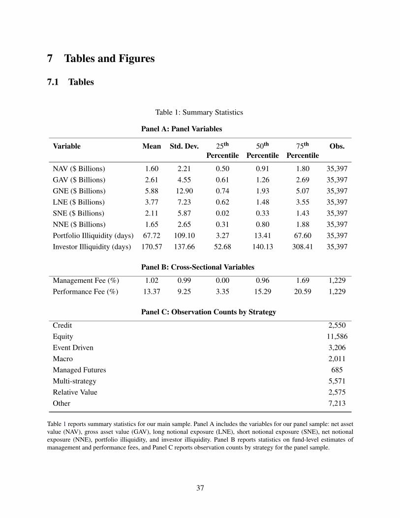
7 Tables and Figures

7.1 Tables

Table 1: Summary Statistics

Panel A: Panel Variables

Variable Mean Std. Dev. 25th 50th 75th Obs.Percentile Percentile Percentile

NAV ($ Billions) 1.60 2.21 0.50 0.91 1.80 35,397GAV ($ Billions) 2.61 4.55 0.61 1.26 2.69 35,397GNE ($ Billions) 5.88 12.90 0.74 1.93 5.07 35,397LNE ($ Billions) 3.77 7.23 0.62 1.48 3.55 35,397SNE ($ Billions) 2.11 5.87 0.02 0.33 1.43 35,397NNE ($ Billions) 1.65 2.65 0.31 0.80 1.88 35,397Portfolio Illiquidity (days) 67.72 109.10 3.27 13.41 67.60 35,397Investor Illiquidity (days) 170.57 137.66 52.68 140.13 308.41 35,397

Panel B: Cross-Sectional Variables

Management Fee (%) 1.02 0.99 0.00 0.96 1.69 1,229Performance Fee (%) 13.37 9.25 3.35 15.29 20.59 1,229

Panel C: Observation Counts by Strategy

Credit 2,550Equity 11,586Event Driven 3,206Macro 2,011Managed Futures 685Multi-strategy 5,571Relative Value 2,575Other 7,213

Table 1 reports summary statistics for our main sample. Panel A includes the variables for our panel sample: net assetvalue (NAV), gross asset value (GAV), long notional exposure (LNE), short notional exposure (SNE), net notionalexposure (NNE), portfolio illiquidity, and investor illiquidity. Panel B reports statistics on fund-level estimates ofmanagement and performance fees, and Panel C reports observation counts by strategy for the panel sample.

37

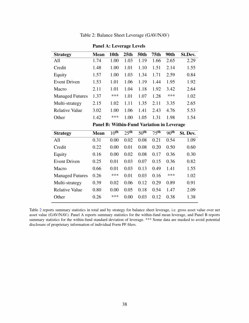
Table 2: Balance Sheet Leverage (GAV/NAV)

Panel A: Leverage Levels

Strategy Mean 10th 25th 50th 75th 90th St.Dev.All 1.74 1.00 1.03 1.19 1.66 2.65 2.29Credit 1.48 1.00 1.01 1.10 1.51 2.14 1.55Equity 1.57 1.00 1.03 1.34 1.71 2.59 0.84Event Driven 1.53 1.01 1.06 1.19 1.44 1.95 1.92Macro 2.11 1.01 1.04 1.18 1.92 3.42 2.64Managed Futures 1.37 *** 1.01 1.07 1.28 *** 1.02Multi-strategy 2.15 1.02 1.11 1.35 2.11 3.35 2.65Relative Value 3.02 1.00 1.06 1.41 2.43 4.76 5.53Other 1.42 *** 1.00 1.05 1.31 1.98 1.54

Panel B: Within-Fund Variation in Leverage

Strategy Mean 10th 25th 50th 75th 90th St. Dev.All 0.31 0.00 0.02 0.08 0.21 0.54 1.09Credit 0.22 0.00 0.01 0.08 0.20 0.50 0.60Equity 0.16 0.00 0.02 0.08 0.17 0.36 0.30Event Driven 0.25 0.01 0.03 0.07 0.15 0.36 0.82Macro 0.66 0.01 0.03 0.13 0.49 1.41 1.55Managed Futures 0.26 *** 0.01 0.03 0.16 *** 1.02Multi-strategy 0.39 0.02 0.06 0.12 0.29 0.89 0.91Relative Value 0.80 0.00 0.05 0.18 0.54 1.47 2.09Other 0.26 *** 0.00 0.03 0.12 0.38 1.38

Table 2 reports summary statistics in total and by strategy for balance sheet leverage, i.e. gross asset value over netasset value (GAV/NAV). Panel A reports summary statistics for the within-fund mean leverage, and Panel B reportssummary statistics for the within-fund standard deviation of leverage. *** Some data are masked to avoid potentialdisclosure of proprietary information of individual Form PF filers.

38

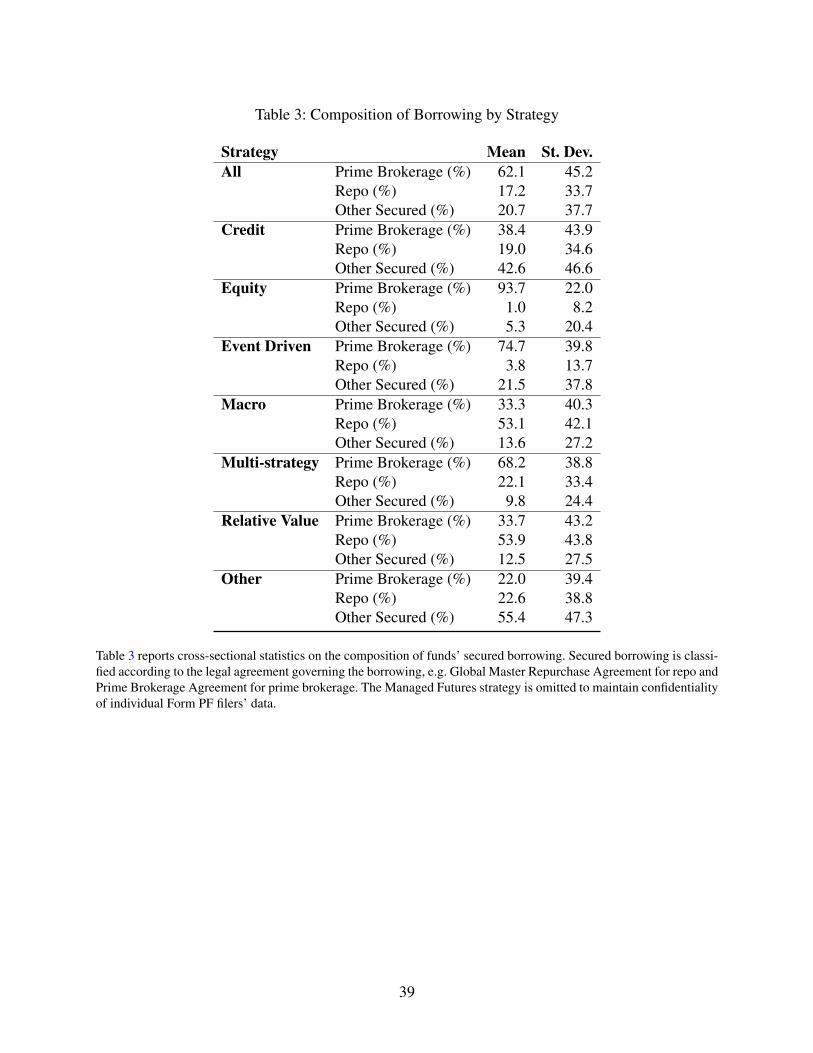
Table 3: Composition of Borrowing by Strategy

Strategy Mean St. Dev.All Prime Brokerage (%) 62.1 45.2

Repo (%) 17.2 33.7Other Secured (%) 20.7 37.7

Credit Prime Brokerage (%) 38.4 43.9Repo (%) 19.0 34.6Other Secured (%) 42.6 46.6

Equity Prime Brokerage (%) 93.7 22.0Repo (%) 1.0 8.2Other Secured (%) 5.3 20.4

Event Driven Prime Brokerage (%) 74.7 39.8Repo (%) 3.8 13.7Other Secured (%) 21.5 37.8

Macro Prime Brokerage (%) 33.3 40.3Repo (%) 53.1 42.1Other Secured (%) 13.6 27.2

Multi-strategy Prime Brokerage (%) 68.2 38.8Repo (%) 22.1 33.4Other Secured (%) 9.8 24.4

Relative Value Prime Brokerage (%) 33.7 43.2Repo (%) 53.9 43.8Other Secured (%) 12.5 27.5

Other Prime Brokerage (%) 22.0 39.4Repo (%) 22.6 38.8Other Secured (%) 55.4 47.3

Table 3 reports cross-sectional statistics on the composition of funds’ secured borrowing. Secured borrowing is classi-fied according to the legal agreement governing the borrowing, e.g. Global Master Repurchase Agreement for repo andPrime Brokerage Agreement for prime brokerage. The Managed Futures strategy is omitted to maintain confidentialityof individual Form PF filers’ data.

39

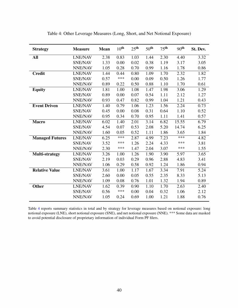
Table 4: Other Leverage Measures (Long, Short, and Net Notional Exposure)

Strategy Measure Mean 10th 25th 50th 75th 90th St. Dev.

All LNE/NAV 2.38 0.83 1.03 1.44 2.30 4.40 3.32SNE/NAV 1.33 0.00 0.02 0.38 1.19 3.17 3.05NNE/NAV 1.05 0.28 0.70 0.99 1.16 1.78 0.86

Credit LNE/NAV 1.44 0.44 0.80 1.09 1.70 2.32 1.82SNE/NAV 0.57 *** 0.00 0.09 0.50 1.26 1.77NNE/NAV 0.89 0.22 0.50 0.88 1.10 1.70 0.61

Equity LNE/NAV 1.81 1.00 1.08 1.47 1.98 3.06 1.29SNE/NAV 0.89 0.00 0.07 0.54 1.11 2.12 1.27NNE/NAV 0.93 0.47 0.82 0.99 1.04 1.21 0.43

Event Driven LNE/NAV 1.40 0.79 1.06 1.23 1.56 2.24 0.73SNE/NAV 0.45 0.00 0.08 0.31 0.64 1.10 0.52NNE/NAV 0.95 0.34 0.70 0.95 1.11 1.41 0.57

Macro LNE/NAV 6.02 1.40 2.01 3.14 6.82 15.55 6.79SNE/NAV 4.54 0.07 0.53 2.08 5.20 14.74 6.25NNE/NAV 1.60 0.05 0.52 1.11 1.86 3.65 1.84

Managed Futures LNE/NAV 6.25 *** 2.87 4.99 7.23 *** 4.82SNE/NAV 3.52 *** 1.26 2.24 4.33 *** 3.81NNE/NAV 2.30 *** 1.47 2.04 3.07 *** 1.55

Multi-strategy LNE/NAV 3.26 1.00 1.26 1.90 3.90 5.97 3.65SNE/NAV 2.19 0.03 0.29 0.96 2.88 4.83 3.41NNE/NAV 1.06 0.29 0.58 0.92 1.24 1.86 0.94

Relative Value LNE/NAV 3.61 1.00 1.17 1.67 3.34 7.91 5.24SNE/NAV 2.60 0.00 0.05 0.55 2.35 8.33 5.13NNE/NAV 1.09 0.08 0.76 1.01 1.32 1.94 0.89

Other LNE/NAV 1.62 0.39 0.90 1.10 1.70 2.63 2.40SNE/NAV 0.56 *** 0.00 0.04 0.32 1.06 2.12NNE/NAV 1.05 0.24 0.69 1.00 1.21 1.88 0.76

Table 4 reports summary statistics in total and by strategy for leverage measures based on notional exposure: longnotional exposure (LNE), short notional exposure (SNE), and net notional exposure (NNE). *** Some data are maskedto avoid potential disclosure of proprietary information of individual Form PF filers.

40

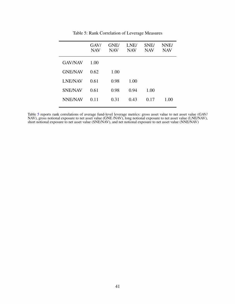
Table 5: Rank Correlation of Leverage Measures

GAV/NAV

GNE/NAV

LNE/NAV

SNE/NAV

NNE/NAV

GAV/NAV 1.00

GNE/NAV 0.62 1.00

LNE/NAV 0.61 0.98 1.00

SNE/NAV 0.61 0.98 0.94 1.00

NNE/NAV 0.11 0.31 0.43 0.17 1.00

Table 5 reports rank correlations of average fund-level leverage metrics: gross asset value to net asset value (GAV/NAV), gross notional exposure to net asset value (GNE /NAV), long notional exposure to net asset value (LNE/NAV),short notional exposure to net asset value (SNE/NAV), and net notional exposure to net asset value (NNE/NAV)

41

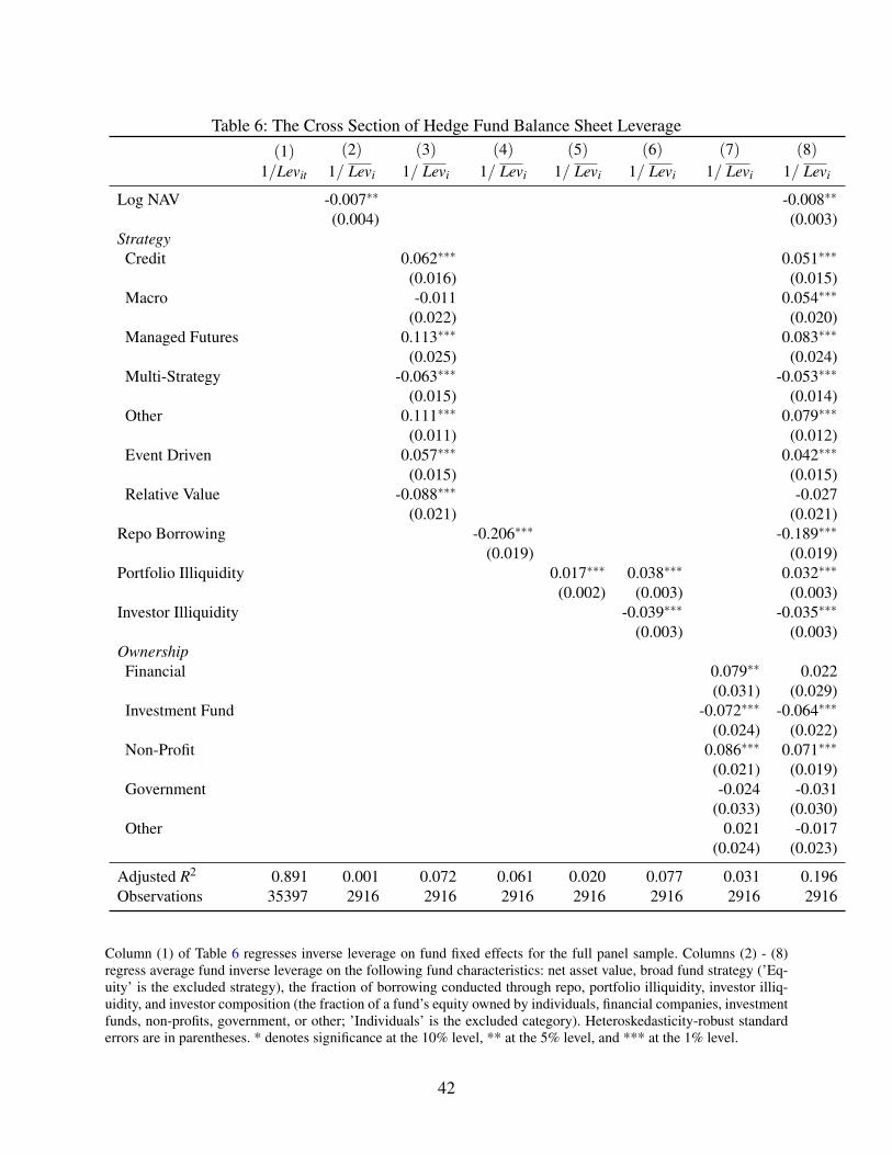
Table 6: The Cross Section of Hedge Fund Balance Sheet Leverage(1)

1/Levit

(2)1/ Levi

(3)1/ Levi

(4)1/ Levi

(5)1/ Levi

(6)1/ Levi

(7)1/ Levi

(8)1/ Levi

Log NAV -0.007∗∗ -0.008∗∗

(0.004) (0.003)StrategyCredit 0.062∗∗∗ 0.051∗∗∗

(0.016) (0.015)Macro -0.011 0.054∗∗∗

(0.022) (0.020)Managed Futures 0.113∗∗∗ 0.083∗∗∗

(0.025) (0.024)Multi-Strategy -0.063∗∗∗ -0.053∗∗∗

(0.015) (0.014)Other 0.111∗∗∗ 0.079∗∗∗

(0.011) (0.012)Event Driven 0.057∗∗∗ 0.042∗∗∗

(0.015) (0.015)Relative Value -0.088∗∗∗ -0.027

(0.021) (0.021)Repo Borrowing -0.206∗∗∗ -0.189∗∗∗

(0.019) (0.019)Portfolio Illiquidity 0.017∗∗∗ 0.038∗∗∗ 0.032∗∗∗

(0.002) (0.003) (0.003)Investor Illiquidity -0.039∗∗∗ -0.035∗∗∗

(0.003) (0.003)OwnershipFinancial 0.079∗∗ 0.022

(0.031) (0.029)Investment Fund -0.072∗∗∗ -0.064∗∗∗

(0.024) (0.022)Non-Profit 0.086∗∗∗ 0.071∗∗∗

(0.021) (0.019)Government -0.024 -0.031

(0.033) (0.030)Other 0.021 -0.017

(0.024) (0.023)

Adjusted R2 0.891 0.001 0.072 0.061 0.020 0.077 0.031 0.196Observations 35397 2916 2916 2916 2916 2916 2916 2916

Column (1) of Table 6 regresses inverse leverage on fund fixed effects for the full panel sample. Columns (2) - (8)regress average fund inverse leverage on the following fund characteristics: net asset value, broad fund strategy (’Eq-uity’ is the excluded strategy), the fraction of borrowing conducted through repo, portfolio illiquidity, investor illiq-uidity, and investor composition (the fraction of a fund’s equity owned by individuals, financial companies, investmentfunds, non-profits, government, or other; ’Individuals’ is the excluded category). Heteroskedasticity-robust standarderrors are in parentheses. * denotes significance at the 10% level, ** at the 5% level, and *** at the 1% level.

42

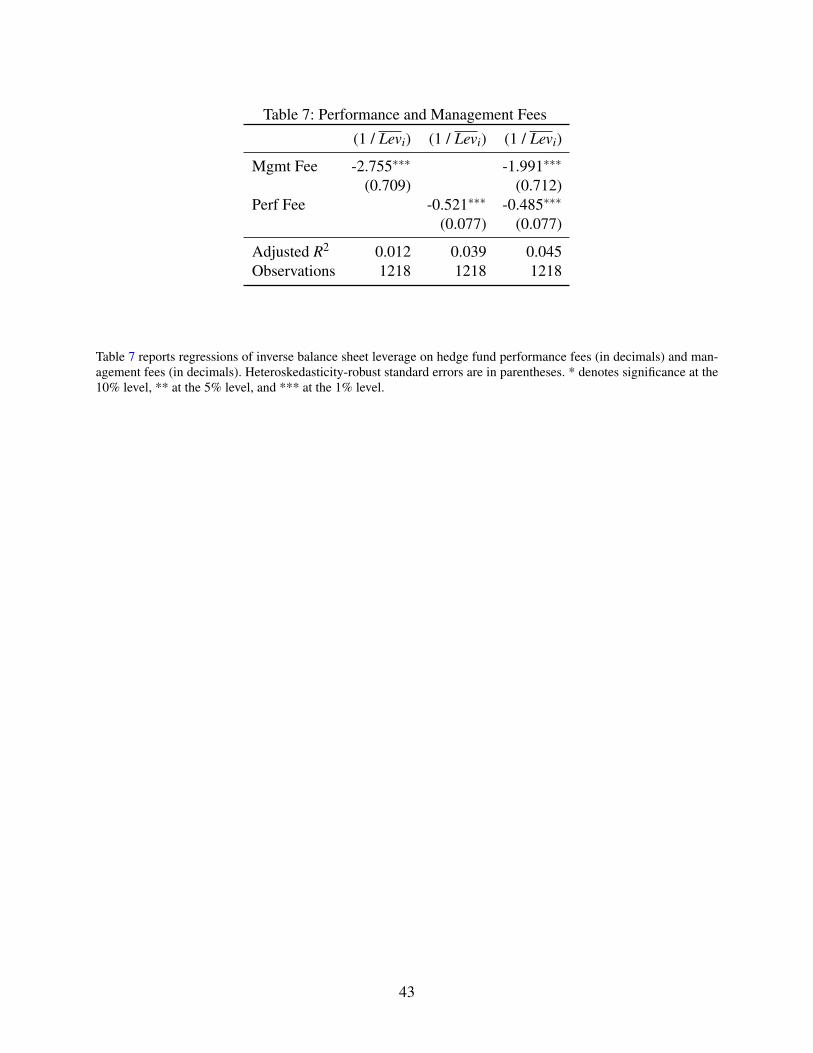
Table 7: Performance and Management Fees

(1 / Levi) (1 / Levi) (1 / Levi)

Mgmt Fee -2.755∗∗∗ -1.991∗∗∗

(0.709) (0.712)Perf Fee -0.521∗∗∗ -0.485∗∗∗

(0.077) (0.077)

Adjusted R2 0.012 0.039 0.045Observations 1218 1218 1218

Table 7 reports regressions of inverse balance sheet leverage on hedge fund performance fees (in decimals) and man-agement fees (in decimals). Heteroskedasticity-robust standard errors are in parentheses. * denotes significance at the10% level, ** at the 5% level, and *** at the 1% level.

43

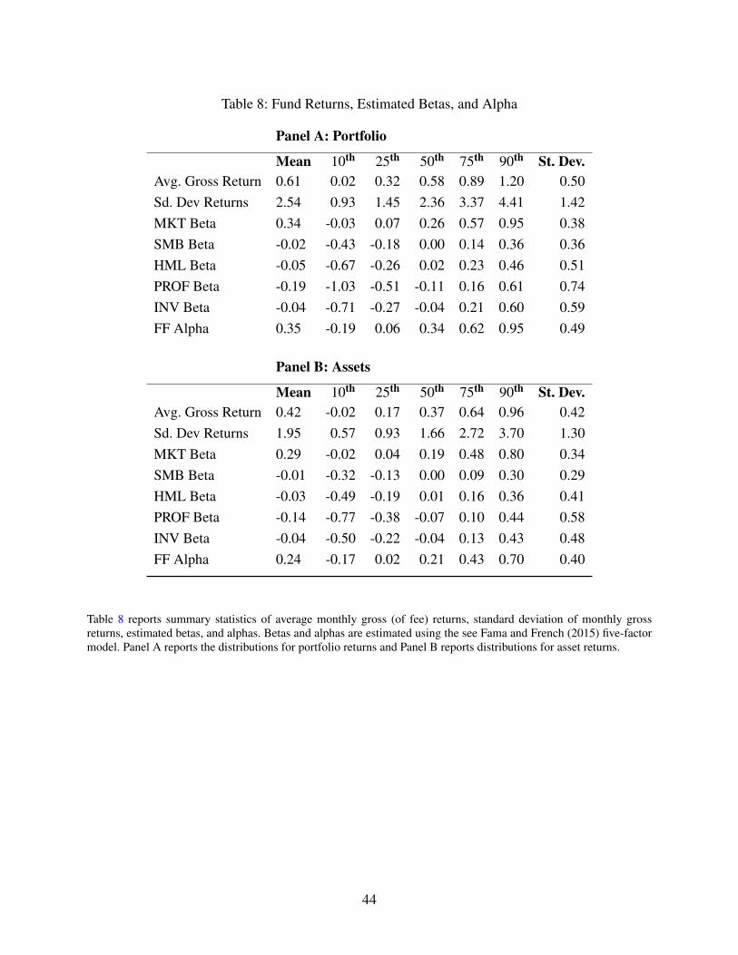
Table 8: Fund Returns, Estimated Betas, and Alpha

Panel A: Portfolio

Mean 10th 25th 50th 75th 90th St. Dev.Avg. Gross Return 0.61 0.02 0.32 0.58 0.89 1.20 0.50Sd. Dev Returns 2.54 0.93 1.45 2.36 3.37 4.41 1.42MKT Beta 0.34 -0.03 0.07 0.26 0.57 0.95 0.38SMB Beta -0.02 -0.43 -0.18 0.00 0.14 0.36 0.36HML Beta -0.05 -0.67 -0.26 0.02 0.23 0.46 0.51PROF Beta -0.19 -1.03 -0.51 -0.11 0.16 0.61 0.74INV Beta -0.04 -0.71 -0.27 -0.04 0.21 0.60 0.59FF Alpha 0.35 -0.19 0.06 0.34 0.62 0.95 0.49

Panel B: Assets

Mean 10th 25th 50th 75th 90th St. Dev.Avg. Gross Return 0.42 -0.02 0.17 0.37 0.64 0.96 0.42Sd. Dev Returns 1.95 0.57 0.93 1.66 2.72 3.70 1.30MKT Beta 0.29 -0.02 0.04 0.19 0.48 0.80 0.34SMB Beta -0.01 -0.32 -0.13 0.00 0.09 0.30 0.29HML Beta -0.03 -0.49 -0.19 0.01 0.16 0.36 0.41PROF Beta -0.14 -0.77 -0.38 -0.07 0.10 0.44 0.58INV Beta -0.04 -0.50 -0.22 -0.04 0.13 0.43 0.48FF Alpha 0.24 -0.17 0.02 0.21 0.43 0.70 0.40

Table 8 reports summary statistics of average monthly gross (of fee) returns, standard deviation of monthly grossreturns, estimated betas, and alphas. Betas and alphas are estimated using the see Fama and French (2015) five-factormodel. Panel A reports the distributions for portfolio returns and Panel B reports distributions for asset returns.

44

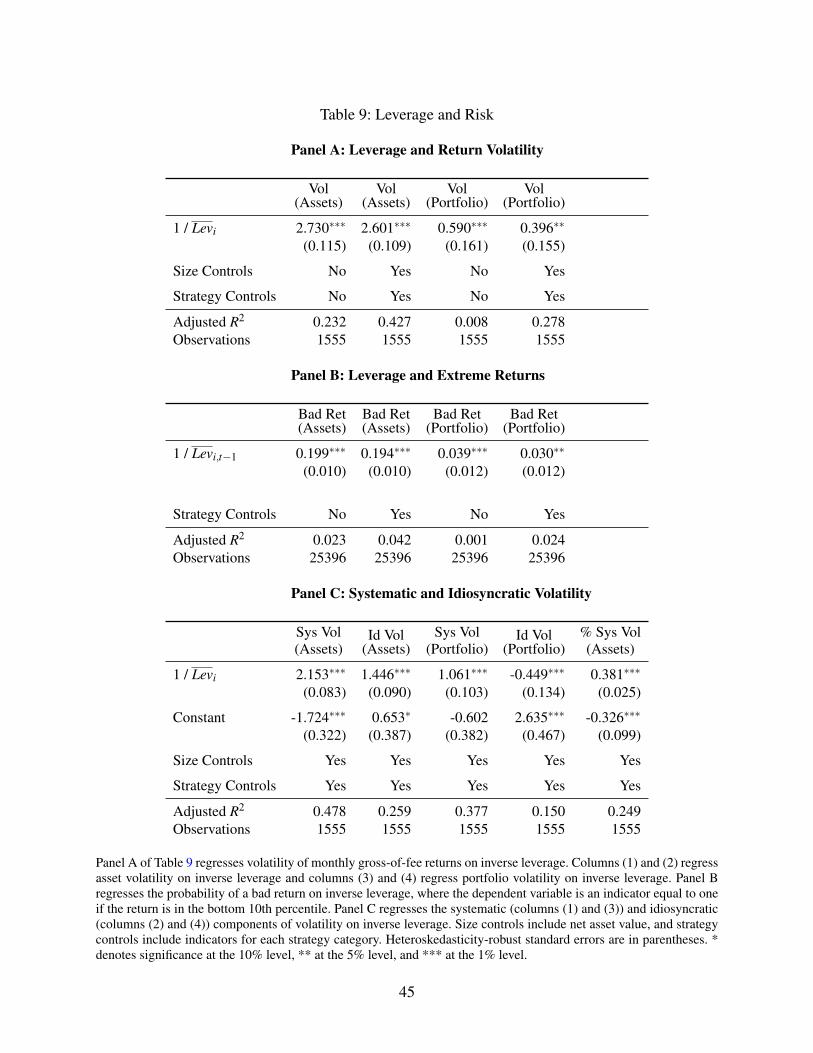
Table 9: Leverage and Risk

Panel A: Leverage and Return Volatility

Vol(Assets)

Vol(Assets)

Vol(Portfolio)

Vol(Portfolio)

1 / Levi 2.730∗∗∗ 2.601∗∗∗ 0.590∗∗∗ 0.396∗∗

(0.115) (0.109) (0.161) (0.155)

Size Controls No Yes No Yes

Strategy Controls No Yes No Yes

Adjusted R2 0.232 0.427 0.008 0.278Observations 1555 1555 1555 1555

Panel B: Leverage and Extreme Returns

Bad Ret(Assets)

Bad Ret(Assets)

Bad Ret(Portfolio)

Bad Ret(Portfolio)

1 / Levi,t−1 0.199∗∗∗ 0.194∗∗∗ 0.039∗∗∗ 0.030∗∗

(0.010) (0.010) (0.012) (0.012)

Strategy Controls No Yes No Yes

Adjusted R2 0.023 0.042 0.001 0.024Observations 25396 25396 25396 25396

Panel C: Systematic and Idiosyncratic Volatility

Sys Vol(Assets)

Id Vol(Assets)

Sys Vol(Portfolio)

Id Vol(Portfolio)

% Sys Vol(Assets)

1 / Levi 2.153∗∗∗ 1.446∗∗∗ 1.061∗∗∗ -0.449∗∗∗ 0.381∗∗∗

(0.083) (0.090) (0.103) (0.134) (0.025)

Constant -1.724∗∗∗ 0.653∗ -0.602 2.635∗∗∗ -0.326∗∗∗

(0.322) (0.387) (0.382) (0.467) (0.099)

Size Controls Yes Yes Yes Yes Yes

Strategy Controls Yes Yes Yes Yes Yes

Adjusted R2 0.478 0.259 0.377 0.150 0.249Observations 1555 1555 1555 1555 1555

Panel A of Table 9 regresses volatility of monthly gross-of-fee returns on inverse leverage. Columns (1) and (2) regressasset volatility on inverse leverage and columns (3) and (4) regress portfolio volatility on inverse leverage. Panel Bregresses the probability of a bad return on inverse leverage, where the dependent variable is an indicator equal to oneif the return is in the bottom 10th percentile. Panel C regresses the systematic (columns (1) and (3)) and idiosyncratic(columns (2) and (4)) components of volatility on inverse leverage. Size controls include net asset value, and strategycontrols include indicators for each strategy category. Heteroskedasticity-robust standard errors are in parentheses. *denotes significance at the 10% level, ** at the 5% level, and *** at the 1% level.

45

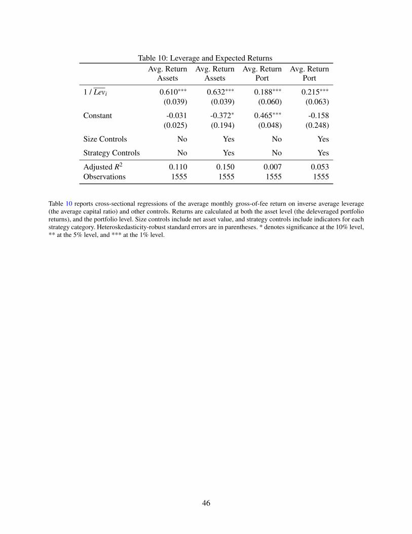
Table 10: Leverage and Expected ReturnsAvg. Return

AssetsAvg. Return

AssetsAvg. Return

PortAvg. Return

Port

1 / Levi 0.610∗∗∗ 0.632∗∗∗ 0.188∗∗∗ 0.215∗∗∗

(0.039) (0.039) (0.060) (0.063)

Constant -0.031 -0.372∗ 0.465∗∗∗ -0.158(0.025) (0.194) (0.048) (0.248)

Size Controls No Yes No Yes

Strategy Controls No Yes No Yes

Adjusted R2 0.110 0.150 0.007 0.053Observations 1555 1555 1555 1555

Table 10 reports cross-sectional regressions of the average monthly gross-of-fee return on inverse average leverage(the average capital ratio) and other controls. Returns are calculated at both the asset level (the deleveraged portfolioreturns), and the portfolio level. Size controls include net asset value, and strategy controls include indicators for eachstrategy category. Heteroskedasticity-robust standard errors are in parentheses. * denotes significance at the 10% level,** at the 5% level, and *** at the 1% level.

46

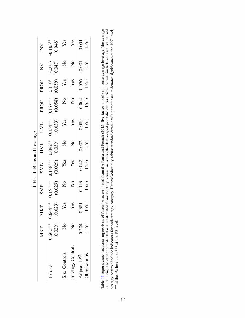
Tabl

e11

:Bet

asan

dL

ever

age

MK

TM

KT

SMB

SMB

HM

LH

ML

PRO

FPR

OF

INV

INV

1/L

evi

0.66

2∗∗∗

0.64

4∗∗∗

0.15

1∗∗∗

0.14

8∗∗∗

0.09

2∗∗

0.13

4∗∗∗

0.16

7∗∗∗

0.11

0∗-0

.017

-0.1

03∗∗

(0.0

29)

(0.0

29)

(0.0

29)

(0.0

29)

(0.0

39)

(0.0

39)

(0.0

58)

(0.0

59)

(0.0

47)

(0.0

48)

Size

Con

trol

sN

oY

esN

oY

esN

oY

esN

oY

esN

oY

es

Stra

tegy

Con

trol

sN

oY

esN

oY

esN

oY

esN

oY

esN

oY

es

Adj

uste

dR

20.

204

0.38

10.

013

0.04

20.

002

0.08

90.

004

0.07

6-0

.001

0.05

1O

bser

vatio

ns15

5515

5515

5515

5515

5515

5515

5515

5515

5515

55

Tabl

e11

repo

rts

cros

s-se

ctio

nalr

egre

ssio

nsof

fact

orbe

tas

estim

ated

from

the

Fam

aan

dFr

ench

(201

5)fiv

e-fa

ctor

mod

elon

inve

rse

aver

age

leve

rage

(the

aver

age

capi

talr

atio

)an

dot

her

cont

rols

.Bet

asar

ees

timat

edfr

omm

onth

lyre

turn

son

asse

ts(t

hede

leve

rage

dpo

rtfo

liore

turn

s).S

ize

cont

rols

incl

ude

neta

sset

valu

e,an

dst

rate

gyco

ntro

lsin

clud

ein

dica

tors

fore

ach

stra

tegy

cate

gory

.Het

eros

keda

stic

ity-r

obus

tsta

ndar

der

rors

are

inpa

rent

hese

s.*

deno

tes

sign

ifica

nce

atth

e10

%le

vel,

**at

the

5%le

vel,

and

***

atth

e1%

leve

l.

47

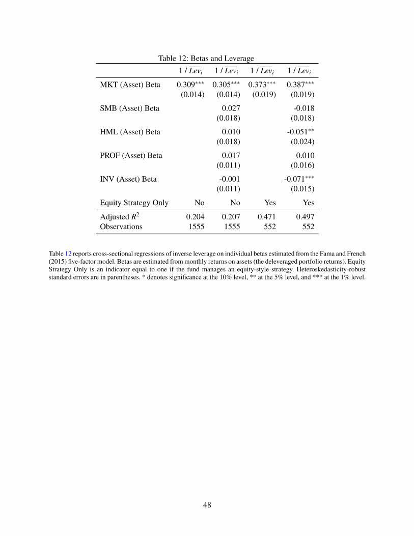
Table 12: Betas and Leverage

1 / Levi 1 / Levi 1 / Levi 1 / Levi

MKT (Asset) Beta 0.309∗∗∗ 0.305∗∗∗ 0.373∗∗∗ 0.387∗∗∗

(0.014) (0.014) (0.019) (0.019)

SMB (Asset) Beta 0.027 -0.018(0.018) (0.018)

HML (Asset) Beta 0.010 -0.051∗∗

(0.018) (0.024)

PROF (Asset) Beta 0.017 0.010(0.011) (0.016)

INV (Asset) Beta -0.001 -0.071∗∗∗

(0.011) (0.015)

Equity Strategy Only No No Yes Yes

Adjusted R2 0.204 0.207 0.471 0.497Observations 1555 1555 552 552

Table 12 reports cross-sectional regressions of inverse leverage on individual betas estimated from the Fama and French(2015) five-factor model. Betas are estimated from monthly returns on assets (the deleveraged portfolio returns). EquityStrategy Only is an indicator equal to one if the fund manages an equity-style strategy. Heteroskedasticity-robuststandard errors are in parentheses. * denotes significance at the 10% level, ** at the 5% level, and *** at the 1% level.

48

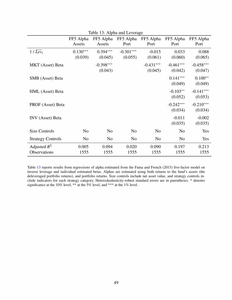
Table 13: Alpha and LeverageFF5 Alpha

AssetsFF5 Alpha

AssetsFF5 Alpha

PortFF5 Alpha

PortFF5 Alpha

PortFF5 Alpha

Port

1 / Levi 0.130∗∗∗ 0.394∗∗∗ -0.301∗∗∗ -0.015 0.033 0.088(0.039) (0.045) (0.055) (0.061) (0.060) (0.065)

MKT (Asset) Beta -0.398∗∗∗ -0.431∗∗∗ -0.461∗∗∗ -0.458∗∗∗

(0.043) (0.045) (0.042) (0.047)

SMB (Asset) Beta 0.141∗∗∗ 0.100∗∗

(0.049) (0.049)

HML (Asset) Beta -0.103∗∗ -0.141∗∗∗

(0.052) (0.053)

PROF (Asset) Beta -0.242∗∗∗ -0.210∗∗∗

(0.034) (0.034)

INV (Asset) Beta -0.011 -0.002(0.035) (0.035)

Size Controls No No No No No Yes

Strategy Controls No No No No No Yes

Adjusted R2 0.005 0.094 0.020 0.090 0.197 0.213Observations 1555 1555 1555 1555 1555 1555

Table 13 reports results from regressions of alpha estimated from the Fama and French (2015) five-factor model oninverse leverage and individual estimated betas. Alphas are estimated using both returns to the fund’s assets (thedeleveraged portfolio returns), and portfolio returns. Size controls include net asset value, and strategy controls in-clude indicators for each strategy category. Heteroskedasticity-robust standard errors are in parentheses. * denotessignificance at the 10% level, ** at the 5% level, and *** at the 1% level.

49

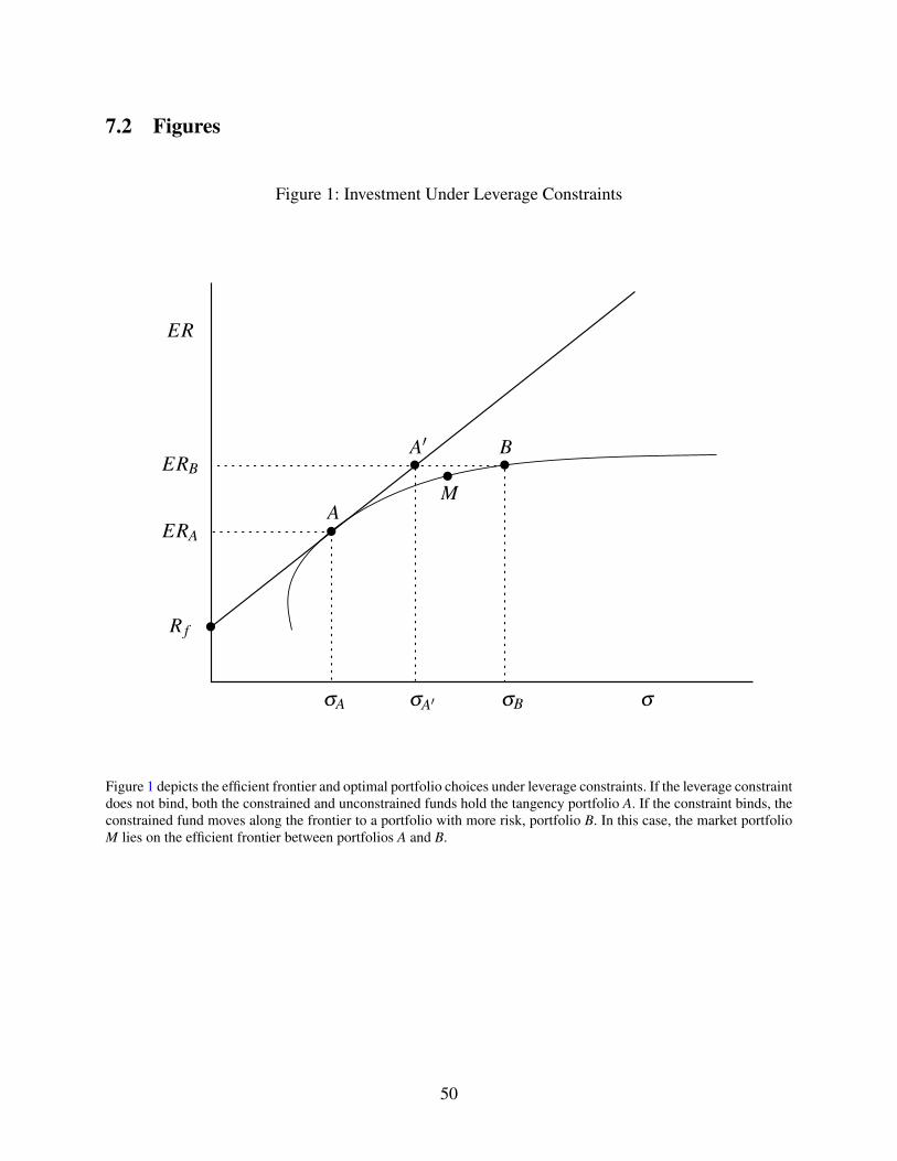
7.2 Figures

Figure 1: Investment Under Leverage Constraints

R f

ERA

ERB

A

A′ B

ER

σ

M

σBσA′σA

Figure 1 depicts the efficient frontier and optimal portfolio choices under leverage constraints. If the leverage constraintdoes not bind, both the constrained and unconstrained funds hold the tangency portfolio A. If the constraint binds, theconstrained fund moves along the frontier to a portfolio with more risk, portfolio B. In this case, the market portfolioM lies on the efficient frontier between portfolios A and B.

50

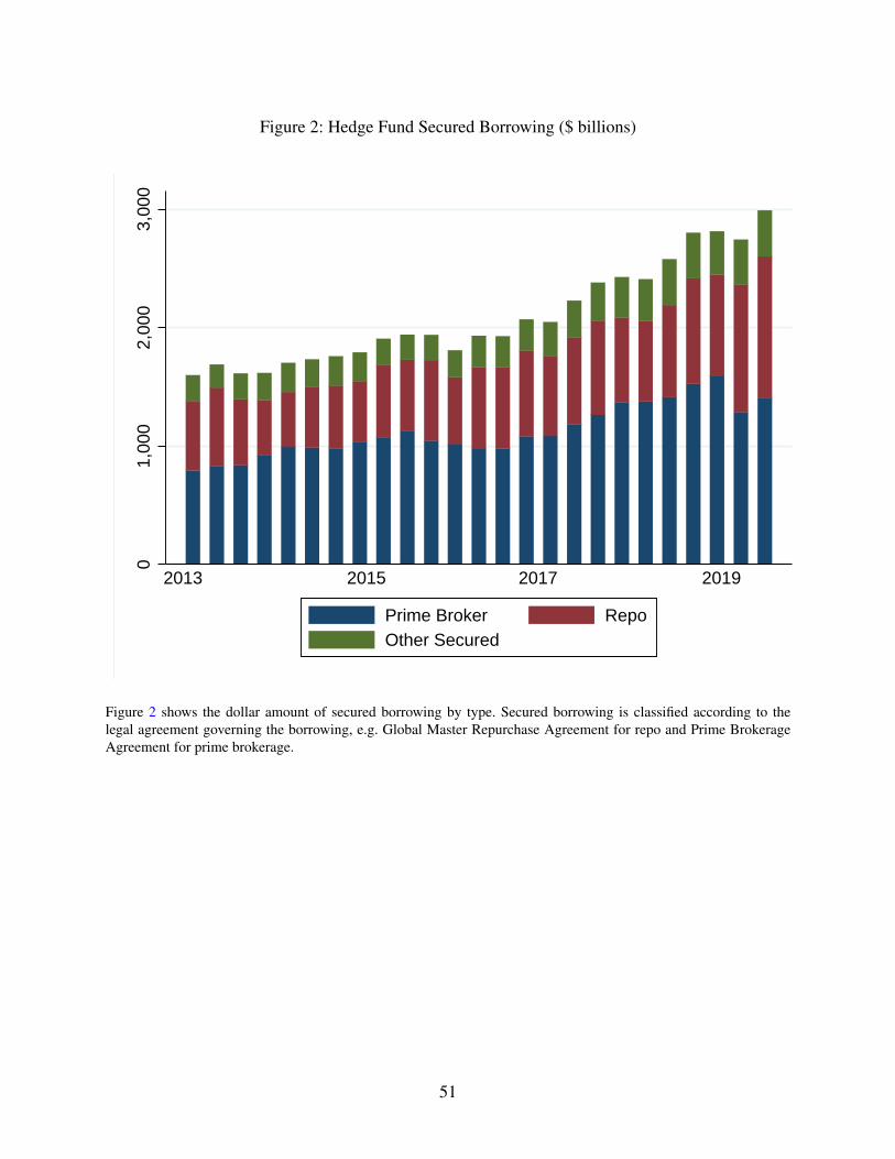
Figure 2: Hedge Fund Secured Borrowing ($ billions)0

1,00

02,

000

3,00

0

2013 2015 2017 2019

Prime Broker RepoOther Secured

Figure 2 shows the dollar amount of secured borrowing by type. Secured borrowing is classified according to thelegal agreement governing the borrowing, e.g. Global Master Repurchase Agreement for repo and Prime BrokerageAgreement for prime brokerage.

51

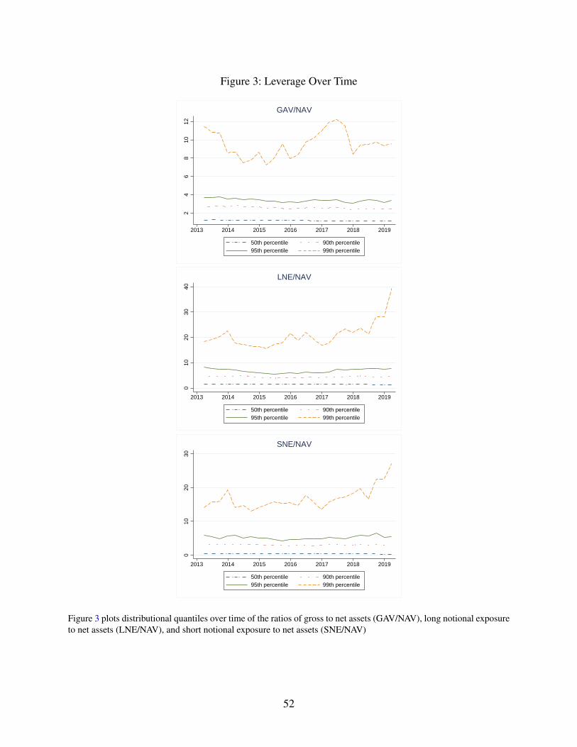
Figure 3: Leverage Over Time

24

68

1012

2013 2014 2015 2016 2017 2018 2019

50th percentile 90th percentile95th percentile 99th percentile

GAV/NAV

010

2030

40

2013 2014 2015 2016 2017 2018 2019

50th percentile 90th percentile95th percentile 99th percentile

LNE/NAV

010

2030

2013 2014 2015 2016 2017 2018 2019

50th percentile 90th percentile95th percentile 99th percentile

SNE/NAV

Figure 3 plots distributional quantiles over time of the ratios of gross to net assets (GAV/NAV), long notional exposureto net assets (LNE/NAV), and short notional exposure to net assets (SNE/NAV)

52

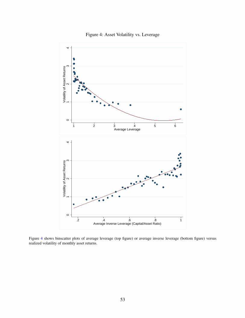
Figure 4: Asset Volatility vs. Leverage

01

23

4V

olat

ility

of A

sset

Ret

urns

1 2 3 4 5 6Average Leverage

01

23

4V

olat

ility

of A

sset

Ret

urns

.2 .4 .6 .8 1Average Inverse Leverage (Capital/Asset Ratio)

Figure 4 shows binscatter plots of average leverage (top figure) or average inverse leverage (bottom figure) versusrealized volatility of monthly asset returns.

53

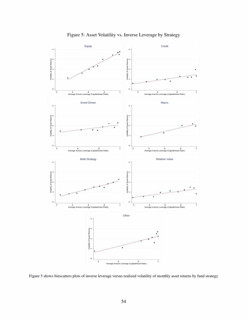
Figure 5: Asset Volatility vs. Inverse Leverage by Strategy

01

23

4V

olat

ility

of A

sset

Ret

urns

.2 .4 .6 .8 1Average Inverse Leverage (Capital/Asset Ratio)

Equity

01

23

4V

olat

ility

of A

sset

Ret

urns

.4 .6 .8 1Average Inverse Leverage (Capital/Asset Ratio)

Credit

01

23

4V

olat

ility

of A

sset

Ret

urns

.4 .6 .8 1Average Inverse Leverage (Capital/Asset Ratio)

Event Driven

01

23

4V

olat

ility

of A

sset

Ret

urns

.2 .4 .6 .8 1Average Inverse Leverage (Capital/Asset Ratio)

Macro

01

23

4V

olat

ility

of A

sset

Ret

urns

.2 .4 .6 .8 1Average Inverse Leverage (Capital/Asset Ratio)

Multi-Strategy

01

23

4V

olat

ility

of A

sset

Ret

urns

.2 .4 .6 .8 1Average Inverse Leverage (Capital/Asset Ratio)

Relative Value

01

23

4V

olat

ility

of A

sset

Ret

urns

.4 .6 .8 1Average Inverse Leverage (Capital/Asset Ratio)

Other

Figure 5 shows binscatters plots of inverse leverage versus realized volatility of monthly asset returns by fund strategy

54

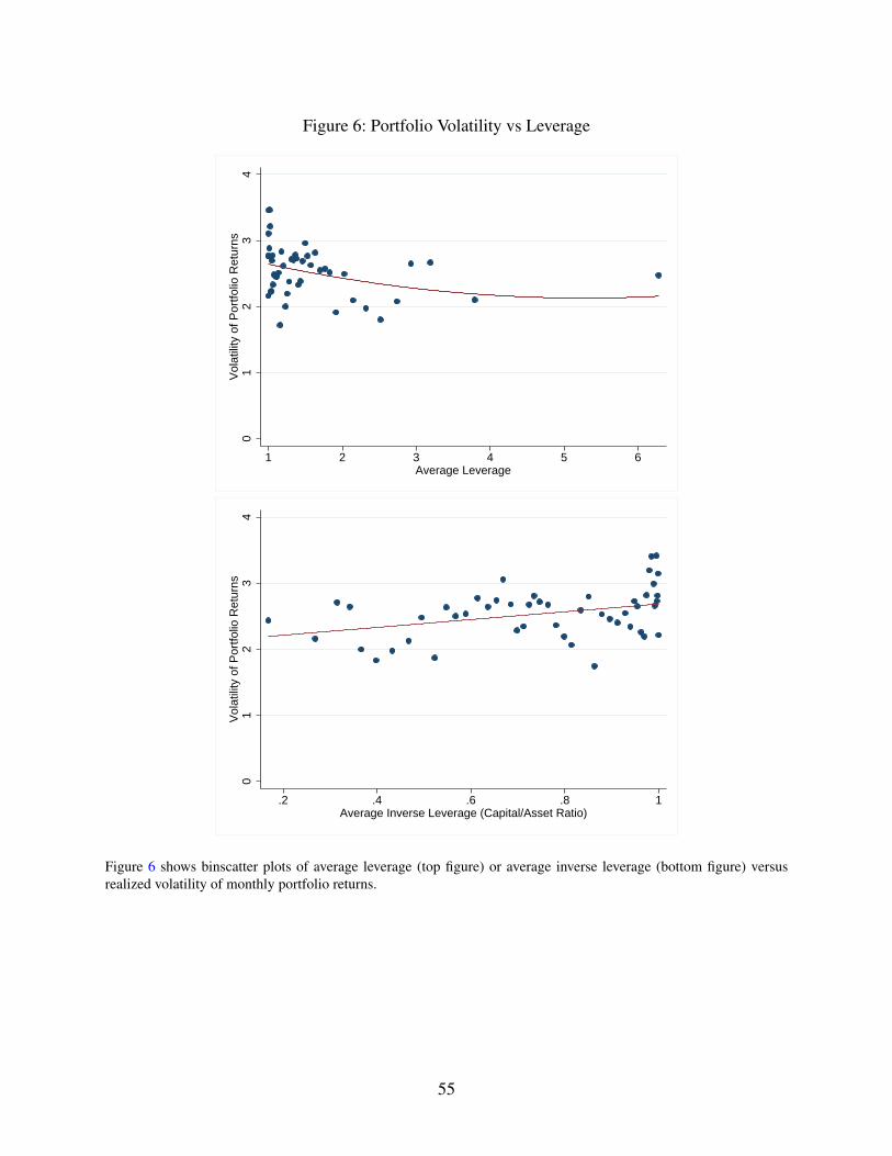
Figure 6: Portfolio Volatility vs Leverage

01

23

4V

olat

ility

of P

ortfo

lio R

etur

ns

1 2 3 4 5 6Average Leverage

01

23

4V

olat

ility

of P

ortfo

lio R

etur

ns

.2 .4 .6 .8 1Average Inverse Leverage (Capital/Asset Ratio)

Figure 6 shows binscatter plots of average leverage (top figure) or average inverse leverage (bottom figure) versusrealized volatility of monthly portfolio returns.

55

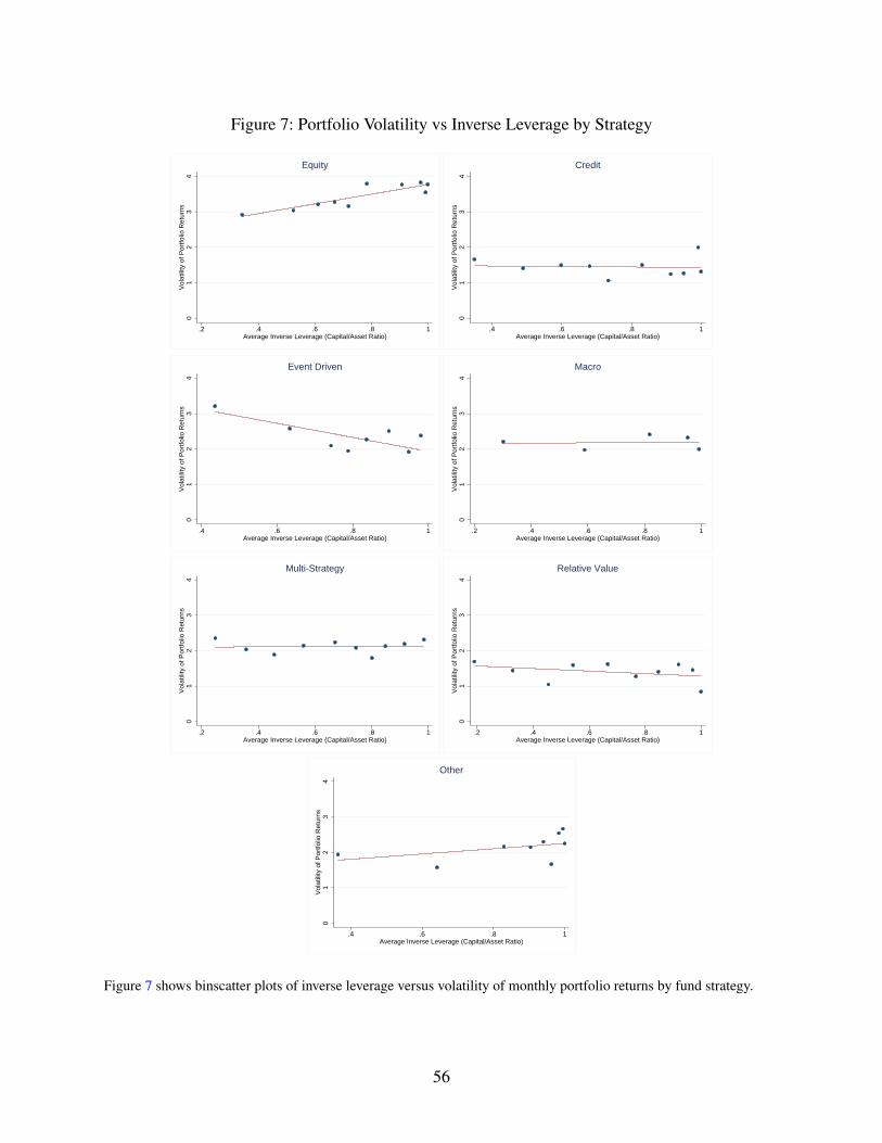
Figure 7: Portfolio Volatility vs Inverse Leverage by Strategy

01

23

4V

olat

ility

of P

ortfo

lio R

etur

ns

.2 .4 .6 .8 1Average Inverse Leverage (Capital/Asset Ratio)

Equity

01

23

4V

olat

ility

of P

ortfo

lio R

etur

ns

.4 .6 .8 1Average Inverse Leverage (Capital/Asset Ratio)

Credit

01

23

4V

olat

ility

of P

ortfo

lio R

etur

ns

.4 .6 .8 1Average Inverse Leverage (Capital/Asset Ratio)

Event Driven

01

23

4V

olat

ility

of P

ortfo

lio R

etur

ns

.2 .4 .6 .8 1Average Inverse Leverage (Capital/Asset Ratio)

Macro

01

23

4V

olat

ility

of P

ortfo

lio R

etur

ns

.2 .4 .6 .8 1Average Inverse Leverage (Capital/Asset Ratio)

Multi-Strategy

01

23

4V

olat

ility

of P

ortfo

lio R

etur

ns

.2 .4 .6 .8 1Average Inverse Leverage (Capital/Asset Ratio)

Relative Value

01

23

4V

olat

ility

of P

ortfo

lio R

etur

ns

.4 .6 .8 1Average Inverse Leverage (Capital/Asset Ratio)

Other

Figure 7 shows binscatter plots of inverse leverage versus volatility of monthly portfolio returns by fund strategy.

56

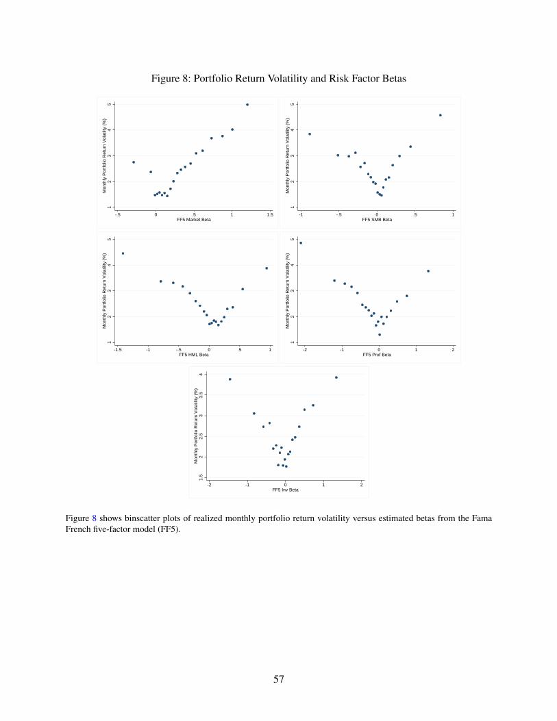
Figure 8: Portfolio Return Volatility and Risk Factor Betas

12

34

5M

onth

ly P

ortfo

lio R

etur

n V

olat

ilty

(%)

-.5 0 .5 1 1.5FF5 Market Beta

12

34

5M

onth

ly P

ortfo

lio R

etur

n V

olat

ility

(%

)

-1 -.5 0 .5 1FF5 SMB Beta

12

34

5M

onth

ly P

ortfo

lio R

etur

n V

olat

ility

(%

)

-1.5 -1 -.5 0 .5 1FF5 HML Beta

12

34

5M

onth

ly P

ortfo

lio R

etur

n V

olat

ility

(%

)

-2 -1 0 1 2FF5 Prof Beta

1.5

22.

53

3.5

4M

onth

ly P

ortfo

lio R

etur

n V

olat

ility

(%

)

-2 -1 0 1 2FF5 Inv Beta

Figure 8 shows binscatter plots of realized monthly portfolio return volatility versus estimated betas from the FamaFrench five-factor model (FF5).

57

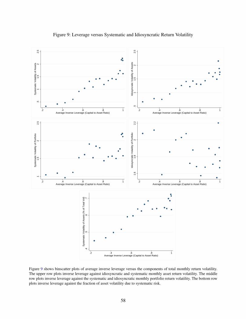
Figure 9: Leverage versus Systematic and Idiosyncratic Return Volatility.5

11.

52

2.5

Sys

tem

atic

Vol

atili

ty o

f Ass

ets

.2 .4 .6 .8 1Average Inverse Leverage (Capital to Asset Ratio)

.51

1.5

22.

5Id

iosy

ncra

tic V

olat

ility

of A

sset

s

.2 .4 .6 .8 1Average Inverse Leverage (Capital to Asset Ratio)

11.

52

2.5

Sys

tem

atic

Vol

atili

ty o

f Por

tfolio

.2 .4 .6 .8 1Average Inverse Leverage (Capital to Asset Ratio)

1.6

1.8

22.

2Id

iosy

ncra

tic V

olat

ility

of P

ortfo

lio

.2 .4 .6 .8 1Average Inverse Leverage (Capital to Asset Ratio)

.4.5

.6.7

Sys

tem

atic

Vol

atili

ty o

f Ass

ets

(% o

f Tot

al V

ol)

.2 .4 .6 .8 1Average Inverse Leverage (Capital to Asset Ratio)

Figure 9 shows binscatter plots of average inverse leverage versus the components of total monthly return volatility.The upper row plots inverse leverage against idiosyncratic and systematic monthly asset return volatility. The middlerow plots inverse leverage against the systematic and idiosyncratic monthly portfolio return volatility. The bottom rowplots inverse leverage against the fraction of asset volatility due to systematic risk.

58

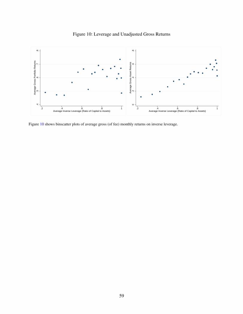
Figure 10: Leverage and Unadjusted Gross Returns.4

.5.6

.7.8

Ave

rage

Gro

ss P

ortfo

lio R

etur

ns

.2 .4 .6 .8 1Average Inverse Leverage (Ratio of Capital to Assets)

0.2

.4.6

.8A

vera

ge G

ross

Ass

et R

etur

ns

.2 .4 .6 .8 1Average Inverse Leverage (Ratio of Capital to Assets)

Figure 10 shows binscatter plots of average gross (of fee) monthly returns on inverse leverage.

59

A Sample Construction

A.1 Fee Estimation

The data do not contain explicit information on the components of hedge fund fees, such as

management and performance fees or high water marks. Instead, only total gross-of-fee and net-of-

fee returns are reported, and we use this information to estimate the performance and management

fees. We limit observations to those with a gross-of-fee return that is at least as large as the net-

of-fee return. This excludes data errors and funds offering rebates. We estimate the management

fee as the maximum fee charged by the fund during negative-return months. The goal is to isolate

the management fee by excluding the performance fee, which would only possibly be charged in

months with positive returns. We then winsorize the estimated management fee at the 5th and 95th

percentiles. Performance fees are usually charged quarterly or annually. To estimate the perfor-

mance fee, we divide the total fee minus the estimated management fee by the total gross return

minus the management fee, all in annual percentages, and winsorize at the 10th and 90th percentiles.

Barth and Monin (2019) show that this procedure produces credible estimates for the management

and performance fees, both unconditionally and based on a matched sample of funds that appear

both Form PF and TASS, the latter of which fee data is collected explicitly.

B Additional Results and Summary Statistics

B.1 Summary Statistics

In this section, we present additional summary statistics for leverage. Panel A of Table B.1

reports the distribution, in aggregate and by strategy, for the inverse of average balance sheet lever-

age (1/Levi). Panel B reports the distribution of the within-fund variation in balance sheet leverage

over time.

B.2 Cross-Sectional Determinants

This section reports additional results for the cross-sectional variation in leverage. Table B.2

repeats the specification in Table 6 but uses as the dependent variable an indicator equal to one if

the fund uses leverage. Table B.3 repeats the same specification, but uses as the dependent variable

60

an indicator equal to one if the fund’s leverage is at or above the 75th percentile.

B.3 Robustness: Leverage and Risk

In this section, we repeat the specifications in columns Panel A of Table 9 using different

measures of leverage: the ratio of long notional exposures to net assets, short notional exposures

to net assets, and gross notional exposure to net assets. To compute inverse leverage for these

measures, we restrict to values greater than 0.01 for LNE/NAV, SNE/NAV, and GNE/NAV. These

results are shown in Table B.4.

B.4 Returns

Tables B.5 and B.6 report regression results related to the time-series variation in returns. Ta-

ble B.5 regresses future returns on the contemporaneous percentage change in leverage. Dependent

variables are the one-quarter ahead, two-quarter ahead, three-quarter ahead, and four-quarter ahead

quarterly returns. Table B.6 reverses the timing of the regressions, and instead regress the contem-

poraneous percentage change in leverage on prior quarterly returns, lagged up to four quarters.

61

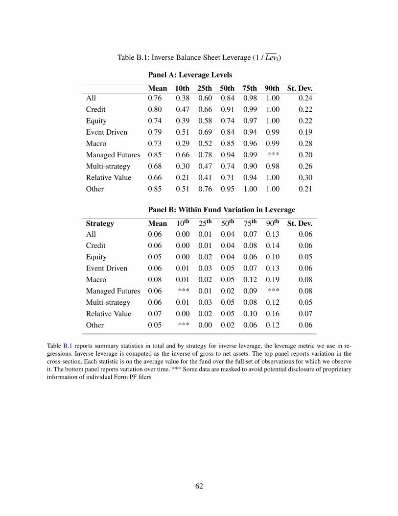
Table B.1: Inverse Balance Sheet Leverage (1 / Levi)

Panel A: Leverage Levels

Mean 10th 25th 50th 75th 90th St. Dev.All 0.76 0.38 0.60 0.84 0.98 1.00 0.24Credit 0.80 0.47 0.66 0.91 0.99 1.00 0.22Equity 0.74 0.39 0.58 0.74 0.97 1.00 0.22Event Driven 0.79 0.51 0.69 0.84 0.94 0.99 0.19Macro 0.73 0.29 0.52 0.85 0.96 0.99 0.28Managed Futures 0.85 0.66 0.78 0.94 0.99 *** 0.20Multi-strategy 0.68 0.30 0.47 0.74 0.90 0.98 0.26Relative Value 0.66 0.21 0.41 0.71 0.94 1.00 0.30Other 0.85 0.51 0.76 0.95 1.00 1.00 0.21

Panel B: Within Fund Variation in Leverage

Strategy Mean 10th 25th 50th 75th 90th St. Dev.All 0.06 0.00 0.01 0.04 0.07 0.13 0.06Credit 0.06 0.00 0.01 0.04 0.08 0.14 0.06Equity 0.05 0.00 0.02 0.04 0.06 0.10 0.05Event Driven 0.06 0.01 0.03 0.05 0.07 0.13 0.06Macro 0.08 0.01 0.02 0.05 0.12 0.19 0.08Managed Futures 0.06 *** 0.01 0.02 0.09 *** 0.08Multi-strategy 0.06 0.01 0.03 0.05 0.08 0.12 0.05Relative Value 0.07 0.00 0.02 0.05 0.10 0.16 0.07Other 0.05 *** 0.00 0.02 0.06 0.12 0.06

Table B.1 reports summary statistics in total and by strategy for inverse leverage, the leverage metric we use in re-gressions. Inverse leverage is computed as the inverse of gross to net assets. The top panel reports variation in thecross-section. Each statistic is on the average value for the fund over the full set of observations for which we observeit. The bottom panel reports variation over time. *** Some data are masked to avoid potential disclosure of proprietaryinformation of individual Form PF filers

62

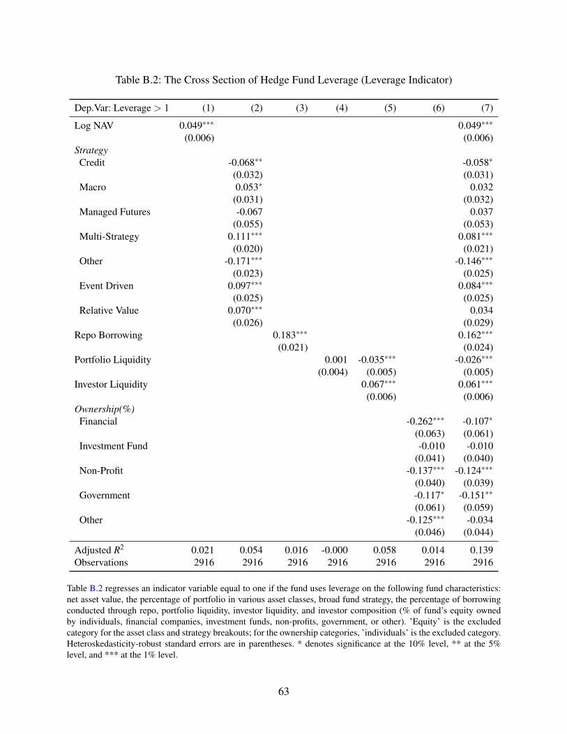
Table B.2: The Cross Section of Hedge Fund Leverage (Leverage Indicator)

Dep.Var: Leverage > 1 (1) (2) (3) (4) (5) (6) (7)

Log NAV 0.049∗∗∗ 0.049∗∗∗

(0.006) (0.006)StrategyCredit -0.068∗∗ -0.058∗

(0.032) (0.031)Macro 0.053∗ 0.032

(0.031) (0.032)Managed Futures -0.067 0.037

(0.055) (0.053)Multi-Strategy 0.111∗∗∗ 0.081∗∗∗

(0.020) (0.021)Other -0.171∗∗∗ -0.146∗∗∗

(0.023) (0.025)Event Driven 0.097∗∗∗ 0.084∗∗∗

(0.025) (0.025)Relative Value 0.070∗∗∗ 0.034

(0.026) (0.029)Repo Borrowing 0.183∗∗∗ 0.162∗∗∗

(0.021) (0.024)Portfolio Liquidity 0.001 -0.035∗∗∗ -0.026∗∗∗

(0.004) (0.005) (0.005)Investor Liquidity 0.067∗∗∗ 0.061∗∗∗

(0.006) (0.006)Ownership(%)Financial -0.262∗∗∗ -0.107∗

(0.063) (0.061)Investment Fund -0.010 -0.010

(0.041) (0.040)Non-Profit -0.137∗∗∗ -0.124∗∗∗

(0.040) (0.039)Government -0.117∗ -0.151∗∗

(0.061) (0.059)Other -0.125∗∗∗ -0.034

(0.046) (0.044)

Adjusted R2 0.021 0.054 0.016 -0.000 0.058 0.014 0.139Observations 2916 2916 2916 2916 2916 2916 2916

Table B.2 regresses an indicator variable equal to one if the fund uses leverage on the following fund characteristics:net asset value, the percentage of portfolio in various asset classes, broad fund strategy, the percentage of borrowingconducted through repo, portfolio liquidity, investor liquidity, and investor composition (% of fund’s equity ownedby individuals, financial companies, investment funds, non-profits, government, or other). ’Equity’ is the excludedcategory for the asset class and strategy breakouts; for the ownership categories, ’individuals’ is the excluded category.Heteroskedasticity-robust standard errors are in parentheses. * denotes significance at the 10% level, ** at the 5%level, and *** at the 1% level.

63

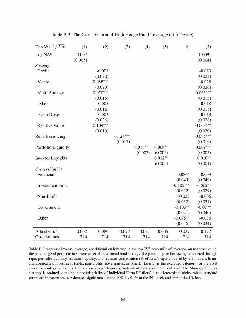
Table B.3: The Cross Section of High Hedge Fund Leverage (Top Decile)

Dep.Var: 1/ Levi (1) (2) (3) (4) (5) (6) (7)

Log NAV 0.007 0.009∗

(0.005) (0.004)StrategyCredit -0.008 -0.013

(0.020) (0.021)Macro -0.088∗∗∗ -0.028

(0.023) (0.026)Multi-Strategy -0.070∗∗∗ -0.063∗∗∗

(0.015) (0.013)Other -0.005 -0.018

(0.016) (0.018)Event Driven -0.003 -0.018

(0.026) (0.026)Relative Value -0.109∗∗∗ -0.069∗∗∗

(0.019) (0.020)Repo Borrowing -0.124∗∗∗ -0.096∗∗∗

(0.017) (0.019)Portfolio Liquidity 0.013∗∗∗ 0.008∗∗ 0.009∗∗∗

(0.003) (0.003) (0.003)Investor Liquidity 0.012∗∗ 0.010∗∗

(0.005) (0.004)Ownership(%)Financial -0.086∗ -0.003

(0.049) (0.049)Investment Fund -0.105∗∗∗ -0.062∗∗

(0.032) (0.029)Non-Profit -0.022 -0.006

(0.032) (0.031)Government -0.103∗∗ -0.077∗

(0.041) (0.040)Other -0.075∗∗ -0.036

(0.036) (0.034)

Adjusted R2 0.002 0.080 0.097 0.027 0.035 0.027 0.172Observations 714 714 714 714 714 714 714

Table B.3 regresses inverse leverage, conditional on leverage in the top 75th percentile of leverage, on net asset value,the percentage of portfolio in various asset classes, broad fund strategy, the percentage of borrowing conducted throughrepo, portfolio liquidity, investor liquidity, and investor composition (% of fund’s equity owned by individuals, finan-cial companies, investment funds, non-profits, government, or other). ’Equity’ is the excluded category for the assetclass and strategy breakouts; for the ownership categories, ’individuals’ is the excluded category. The Managed Futuresstrategy is omitted to maintain confidentiality of individual Form PF filers’ data. Heteroskedasticity-robust standarderrors are in parentheses. * denotes significance at the 10% level, ** at the 5% level, and *** at the 1% level.

64

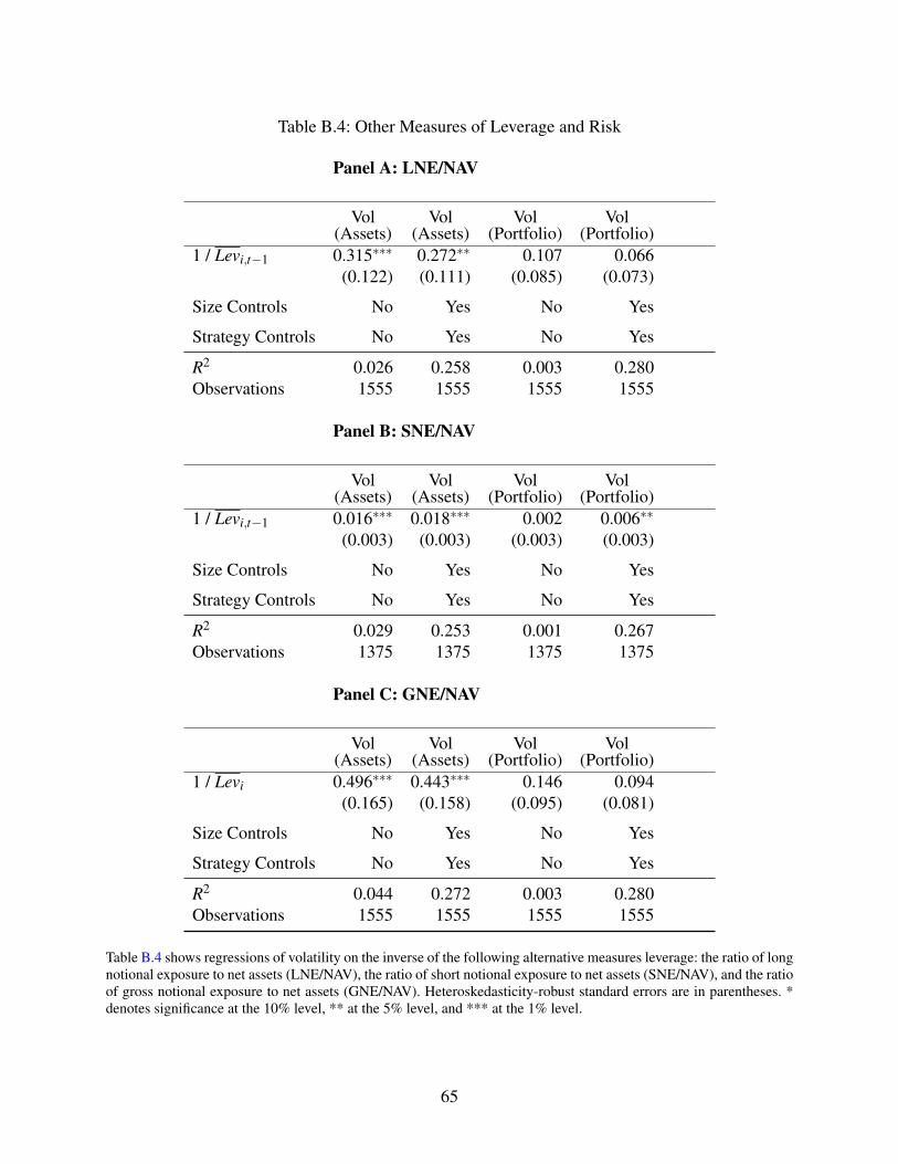
Table B.4: Other Measures of Leverage and Risk

Panel A: LNE/NAV

Vol(Assets)

Vol(Assets)

Vol(Portfolio)

Vol(Portfolio)

1 / Levi,t−1 0.315∗∗∗ 0.272∗∗ 0.107 0.066(0.122) (0.111) (0.085) (0.073)

Size Controls No Yes No Yes

Strategy Controls No Yes No Yes

R2 0.026 0.258 0.003 0.280Observations 1555 1555 1555 1555

Panel B: SNE/NAV

Vol(Assets)

Vol(Assets)

Vol(Portfolio)

Vol(Portfolio)

1 / Levi,t−1 0.016∗∗∗ 0.018∗∗∗ 0.002 0.006∗∗

(0.003) (0.003) (0.003) (0.003)

Size Controls No Yes No Yes

Strategy Controls No Yes No Yes

R2 0.029 0.253 0.001 0.267Observations 1375 1375 1375 1375

Panel C: GNE/NAV

Vol(Assets)

Vol(Assets)

Vol(Portfolio)

Vol(Portfolio)

1 / Levi 0.496∗∗∗ 0.443∗∗∗ 0.146 0.094(0.165) (0.158) (0.095) (0.081)

Size Controls No Yes No Yes

Strategy Controls No Yes No Yes

R2 0.044 0.272 0.003 0.280Observations 1555 1555 1555 1555

Table B.4 shows regressions of volatility on the inverse of the following alternative measures leverage: the ratio of longnotional exposure to net assets (LNE/NAV), the ratio of short notional exposure to net assets (SNE/NAV), and the ratioof gross notional exposure to net assets (GNE/NAV). Heteroskedasticity-robust standard errors are in parentheses. *denotes significance at the 10% level, ** at the 5% level, and *** at the 1% level.

65

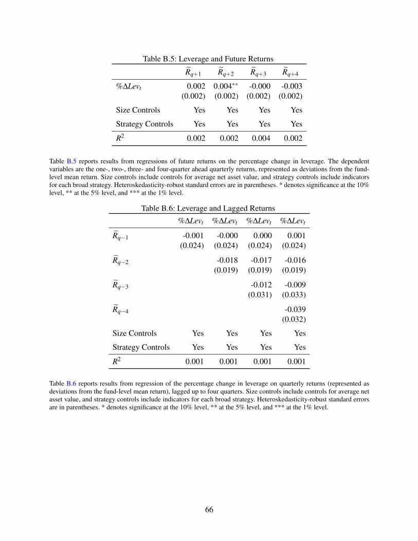
Table B.5: Leverage and Future Returns

R̃q+1 R̃q+2 R̃q+3 R̃q+4

%∆Levt 0.002 0.004∗∗ -0.000 -0.003(0.002) (0.002) (0.002) (0.002)

Size Controls Yes Yes Yes Yes

Strategy Controls Yes Yes Yes Yes

R2 0.002 0.002 0.004 0.002

Table B.5 reports results from regressions of future returns on the percentage change in leverage. The dependentvariables are the one-, two-, three- and four-quarter ahead quarterly returns, represented as deviations from the fund-level mean return. Size controls include controls for average net asset value, and strategy controls include indicatorsfor each broad strategy. Heteroskedasticity-robust standard errors are in parentheses. * denotes significance at the 10%level, ** at the 5% level, and *** at the 1% level.

Table B.6: Leverage and Lagged Returns

%∆Levt %∆Levt %∆Levt %∆Levt

R̃q−1 -0.001 -0.000 0.000 0.001(0.024) (0.024) (0.024) (0.024)

R̃q−2 -0.018 -0.017 -0.016(0.019) (0.019) (0.019)

R̃q−3 -0.012 -0.009(0.031) (0.033)

R̃q−4 -0.039(0.032)

Size Controls Yes Yes Yes Yes

Strategy Controls Yes Yes Yes Yes

R2 0.001 0.001 0.001 0.001

Table B.6 reports results from regression of the percentage change in leverage on quarterly returns (represented asdeviations from the fund-level mean return), lagged up to four quarters. Size controls include controls for average netasset value, and strategy controls include indicators for each broad strategy. Heteroskedasticity-robust standard errorsare in parentheses. * denotes significance at the 10% level, ** at the 5% level, and *** at the 1% level.

66