Level of Service Model for Bicycle Riders - ABC |...
82
Level of Service Model for Bicycle Riders Prepared for Department of Transport and Main Roads
Transcript of Level of Service Model for Bicycle Riders - ABC |...

Level of Service Model for Bicycle Riders
Prepared for Department of Transport and Main Roads

Level of Service Model for Bicycle Riders
0027 TMR LEVEL OF SERVICE MODEL (FINAL-2).DOCX Page i
Contents Executive Summary .................................................................................................... iv
1 Introduction ........................................................................................................... 1
1.1 Scope of study .............................................................................................. 11.2 Objectives ..................................................................................................... 11.3 Structure of this report .................................................................................. 2
2 Background ........................................................................................................... 3
2.1 Terminology .................................................................................................. 32.2 Previous studies ........................................................................................... 42.3 Data requirements ........................................................................................ 92.4 Limitations of existing approaches ............................................................. 102.5 Which model is ‘best’? ................................................................................ 10
3 Methodology ........................................................................................................ 13
3.1 Outline ........................................................................................................ 133.2 Online survey .............................................................................................. 133.3 Stated preference survey ........................................................................... 13
4 Survey results ..................................................................................................... 18
4.1 Summary statistics ..................................................................................... 184.2 Trip context ................................................................................................. 224.3 Route choices ............................................................................................. 254.4 Delayed passing ......................................................................................... 274.5 On-road facilities ......................................................................................... 30
5 Discrete choice model ........................................................................................ 33
5.1 Outline ........................................................................................................ 335.2 Discrete choice models .............................................................................. 335.3 Model estimation ........................................................................................ 335.4 Dataset ....................................................................................................... 355.5 Results ........................................................................................................ 355.6 Model adjustments ..................................................................................... 415.7 LOS mapping .............................................................................................. 425.8 Developing the composite route LOS measurement ................................. 43
6 Model implementation ........................................................................................ 44
7 Sensitivity testing ............................................................................................... 48
7.1 Outline ........................................................................................................ 487.2 Motor vehicle interactions ........................................................................... 487.3 Delay .......................................................................................................... 517.4 Facility type ................................................................................................. 537.5 Traffic volumes ........................................................................................... 567.6 Speed limits ................................................................................................ 58
Level of Service Model for Bicycle Riders
0027 TMR LEVEL OF SERVICE MODEL (FINAL-2).DOCX Page ii
7.7 Parking ....................................................................................................... 607.8 Summary .................................................................................................... 60
8 Route choices ...................................................................................................... 61
8.1 Outline ........................................................................................................ 618.2 Example 1: Shared path vs roadway .......................................................... 618.3 Example 2: On-road main road vs quiet street ........................................... 648.4 Example 3: On-road vs On-road with bicycle lanes ................................... 658.5 Example 3: On-road vs On-road with protected bicycle lanes ................... 65
9 Practical examples .............................................................................................. 67
9.1 Outline ........................................................................................................ 679.2 Link examples ............................................................................................. 679.3 Route examples .......................................................................................... 69
10 Further work ........................................................................................................ 73
10.1 Intersection LOS ......................................................................................... 7310.2 Revealed preference calibration ................................................................. 73
11 References ........................................................................................................... 76

Level of Service Model for Bicycle Riders
0027 TMR LEVEL OF SERVICE MODEL (FINAL-2).DOCX Page iii
Document history and status
Revision Date issued Author Revision type
1 5/11/2013 C. Munro Draft
2 6/11/2013 C. Munro Final
3 22/11/2013 C. Munro Minor model respecification
Distribution of Copies
Revision Media Issued to
1 PDF ARRB, Department of Transport & Main Roads
2 PDF Department of Transport & Main Roads
3 PDF Department of Transport & Main Roads
Printed: 22 November 2013
Last saved: 6 November 2013 09:18 PM
File name: 0027 TMR Level of Service Model (Final-2).docx
Project manager: C. Munro
Name of organisation: ARRB / Department of Transport & Main Roads
Name of project: Level of Service Model for Bicycle Riders
Project number: 0027

Level of Service Model for Bicycle Riders
0027 TMR LEVEL OF SERVICE MODEL (FINAL-2).DOCX Page iv
Executive Summary This report describes the development of a mid-block level of service (LOS) model for
bicycle riders. The model has the objective of providing the non-technical practitioner with a
means to rapidly estimate the LOS of a current link or route, and of the likely LOS with
different design alternatives. Furthermore, the model is capable of estimating the
proportion of demand that will use competing facilities. This includes the ability to predict
demand on competing routes with different types of bicycle facilities, traffic volumes and
frequency of delay.
The model was developed from stated preference surveys of bicycle riders in Queensland
and Victoria. The model is sensitive to the following parameters:
facility type (shared path, cycleway, on-road without bicycle lanes, on-road bicycle
lanes, on-road protected bicycle lanes)
frequency of delay due to interaction with other path/road users,
interactions with other path users (cyclists, pedestrians),
car volumes,
bus volumes,
presence of kerbside parking,
speed limits (50, 60, 80 km/h),
Models for self-identified cautious and confident riders were developed, such that the
analyst can consider the impact of a treatment on both groups independently.
In order to determine the frequency of user interactions a path interactions model is
incorporated, based on earlier research. This interactions model provides forecasts of the
frequency with which a rider will be delayed or interact with other users on shared paths
and cycleways. This interactions model allows users to examine the impact of path width
and modal segregation (pedestrians, bicycle riders) on the frequency of interactions. In
turn, the LOS model then allows to examine the implications these interactions have on
path LOS.
The stated preference surveys were completed by 443 individuals in Queensland and 602
individuals in Victoria, giving a total sample of 1,045 individuals for estimating a discrete
choice model. The model behaves in a way broadly consistent with expectations. Some of
the key findings from the model were:
Riders are highly sensitive to the provision of dedicated on-road cycling
infrastructure; cautious riders in particular are prepared to divert to use routes with
dedicated provision.
Off-road paths and particularly on-road protected bicycle lanes are strongly
preferred to roads without facilities.
Riders are far more sensitive to interacting with buses on roads than with cars.
Riders prefer on-road routes without kerbside parking.

Level of Service Model for Bicycle Riders
0027 TMR LEVEL OF SERVICE MODEL (FINAL-2).DOCX Page v
Riders are sensitive to delays on paths and roads where they occur every 4-6
minutes or more often. Beyond this range they are largely insensitive to delays.
Riders on shared paths are sensitive to passing pedestrians, but not to passing
other bicycle riders.
Two avenues for further research are suggested:
intersection levels of service, and
calibration of the model using revealed preference (observed route choice) data.

Level of Service Model for Bicycle Riders
0027 TMR LEVEL OF SERVICE MODEL (FINAL-2).DOCX Page 1
1 Introduction 1.1 Scope of study CDM Research was appointed by ARRB on behalf of the Queensland Department of
Transport and Main Roads to develop a mid-block level of service (LOS) model for bicycle
riders. This study follows from an earlier project examining the “capacity” of shared paths
and cycleways1. That earlier study had the objective of understanding the maximum
throughput of a path given specified cyclist and pedestrian demand, directional splits and
path width. This maximum throughput represented what was considered to be the limit of
comfortable and safe passage of path users.
The present study extends upon that earlier study by developing a model of cyclist level of
service that considers not just likelihood of delay, but also the frequency of encountering
other path users and, in on-road environments, the frequency of overtaking cars and buses,
their speed and the presence of dedicated cycling facilities. The purpose of this model is to
provide objective, empirically sound guidance on path width, modal segregation
(pedestrians, bicycle riders) and on-road facilities.
The main limitation of this study is that intersections are not considered (except insofar as
they influence the frequency of delay). Given that the majority of police-reported cyclist
crashes occur at intersections, and that anecdotally riders report a strong willingness to
divert around particularly onerous intersections, we would expect a complete picture of
route LOS should assign significant weight to these intersection characteristics. However,
the scope of this project was limited intentionally to mid-block locations, as it is here that the
principle issue of conflict and capacity were deemed most relevant.
1.2 Objectives The main objective of this study was to assist planners in understanding the relative merits
of different types of enroute cycling infrastructure. This included consideration of levels of
separation from traffic (e.g. on-road bicycle lanes, protected bicycle lanes and shared paths
away from roads) and the main characteristics of roadways (e.g. traffic volume and speed).
Furthermore, an understanding of the likely impact of delays on paths would have on
discouraging riders (and diverting them onto other routes) was sought. The project
outcome was to provide guidance on these issues and a supporting spreadsheet-based
model suitable for the non-technical practitioner to be able to quickly test different
scenarios.
1 Sinclair Knight Merz (2010) Bicycle and Pedestrian Capacity Model: North Brisbane Cycleway Investigation, prepared for Queensland Department of Transport and Main Roads.

Level of Service Model for Bicycle Riders
0027 TMR LEVEL OF SERVICE MODEL (FINAL-2).DOCX Page 2
1.3 Structure of this report This report is structured as follows:
Chapter 2 briefly reviews the research on cyclist levels of service, and the
application of these models to Queensland.
Chapter 3 describes the survey methodology adopted to obtain primary data for
developing the level of service model.
Chapter 4 presents results of the survey.
Chapter 5 describes the estimation and interpretation of the discrete choice model
based on the stated preference surveys.
Chapter 6 briefly describes the spreadsheet implementation of the model, and how
it can be used by practitioners.
Chapter 7 presents a series of sensitivity tests, to illustrate the plausibility of the
model.
Chapter 8 discusses the probabilistic nature of the model, and how this
characteristic can be useful in understanding the trade-offs that riders make
between different route options.
Chapter 9 describes a series of typical real-world route planning studies, and how
the model could be useful in identifying and prioritising design options.
Chapter 10 offers two avenues for further work, which may increase the capability
of the model and confidence in the model behaviour.

Level of Service Model for Bicycle Riders
0027 TMR LEVEL OF SERVICE MODEL (FINAL-2).DOCX Page 3
2 Background 2.1 Terminology
2.1.1 Level of service
Level of service is a widely used concept within traffic engineering. In that context it refers
to the flow of traffic; LOS A refers to free flow conditions (i.e. no delays) and LOS F refers to
severe congestion (i.e. long delays). By this definition LOS can be readily measured as the
difference between the observed travel time and that under free flow conditions. LOS is
independent of issues such as pavement quality, scenery, road type and so on; it is based
purely on the notion that a motorist wishes to travel from A to B as rapidly as possible.
For bicycle riders the LOS will ve more complicated for two reasons:
bicycle riders will perceive their “comfort” as being dependent on far more than just
travel time, and
bicycle riders are a heterogenous group; preferences for different route types and
tolerance for adverse conditions (e.g. busy motor traffic) will differ widely among
individuals, and even within individuals across purposes.
We consider here level of service to be analogous to “comfort” or “satisfaction” for bicycle
riders. Clearly, this comfort will be strongly affected by – for example – motor vehicle traffic.
Furthermore, the way in which riders perceive the presence of motor vehicle traffic will differ
between “confident” road riders and more “cautious” riders. Furthermore, just as values of
travel time will vary between purposes for motorised modes, so too would we expect riders
to assign different tradeoffs between time, distance and en-route facilities depending on
their travel purpose (and, indeed, their “mood” more generally).
2.1.2 Capacity
In the earlier Sinclair Knight Merz study for which this project is the basis, the interest was
in identifying appropriate path widths to design for future growth in cycling (SKM, 2010).
The emphasis was on identifying the maximum practical throughput shared paths and
cycleways of given widths could accept. This was referred to as “capacity”. It was
assumed that once capacity was reached (or approached) riders would (a) feel increasing
dissatisfied, and (b) may be tempted to make unsafe overtaking and hence risk injury to
themselves and other path users. The threshold by which capacity was defined was based
on an arbitrary tolerance of delay of 5 minute headways (i.e. 12 delays per hour). In effect,
this represents a threshold level of service rather than absolute capacity (i.e. maximum
flow). As such, the term capacity is not recommended for use in this discussion. Rather,
the maximum tolerable demand is instead whatever LOS is deemed to represent a marginal
condition. Borrowing from motorist LOS this would usually be the threshold when LOS
increases from D to C.

Level of Service Model for Bicycle Riders
0027 TMR LEVEL OF SERVICE MODEL (FINAL-2).DOCX Page 4
2.2 Previous studies There have been a number of LOS models developed for measuring mid-block cycling
conditions. The main characteristics of these models are summarised in Table 2.1. An
extension of the US BLOS (Bicycle Level of Service) model has also been developed for
intersections; for simplicity this model is not considered in this discussion.
Table 2.1: Summary of mid-block LOS models
BCI (Bicycle Compatibility
Index)
BLOS (Bicycle Level of Service)
Danish BLOS VicRoads/BNV
Reference FHWA‐RD‐98‐095 TRR 1578 Trafitec Unpublished
Year 1997 1997 2007 2012
Location Chapel Hill NC, Olympia WA, Austin TX (USA)
Florida (USA) Denmark Victoria
Usage FHWA, , ≥2 states ≥17 states Unknown VicRoads SmartRoads (network operating plans)
Methodology Ranking of stationary video clips (n=202)
Scoring of segments across pre‐determined course (n=150)
Scoring of moving video clips table from cyclist perspective (n=407)
Professional judgement
Parameters
Bicycle lane
Shoulder
Kerbside lane width
Traffic volume
Heavy vehicles
No. of traffic lanes
Speed limit
Adjacent land uses
Presence of parking
Parking occupancy
Parking time limit
Parking lane width
Pavement condition

Level of Service Model for Bicycle Riders
0027 TMR LEVEL OF SERVICE MODEL (FINAL-2).DOCX Page 5
BCI (Bicycle Compatibility
Index)
BLOS (Bicycle Level of Service)
Danish BLOS VicRoads/BNV
Pedestrians
Presence of bus stops
Left‐turning volumes
Comment Stationary roadside video may not be sufficiently realistic
Adopted for use in NCHRP‐616 and upcoming 2010 HCM Log‐volume is used (linear for BCI)
Most sophisticated modelling specification. Wide range of cyclist facilities (more akin to Queensland situation)
Scoring system based on professional judgement
Three methods calibrated their models based on either video clips (BCI, Danish BLOS) of
different types of route or actual riding of different routes (BLOS). The latter feels
somewhat more reliable, given that videos have a more constrained field of view than the
human eye (and more than just visual stimuli are important in a cyclists’ level of comfort).
These methods all have in common two significant methodological constraints, however:
the variables are not always uncorrelated (e.g. traffic volume is often related to
traffic speed), and
extraneous factors may have an impact of the respondent ratings (e.g. the section
of route with a bike path may also have lots of trees and so seem ‘more pleasant’).
How significant these issues are is unclear without having access to the raw data and
videos. Nonetheless, experimental design methods do exist which can avoid (or at least
minimise) these problems.
We now review each of the LOS methods in more detail.
2.2.1 Bicycle Safety Index Rating
The Bicycle Safety Index Rating (BSIR) was developed to predict cyclist-motorist crash
exposure (Epperson, 1994). The method, developed in Florida (USA), is based on the
assertion that LOS is directly correlated with the objective likelihood of crash involvement.
It is not clear that the model has been used in practice, and seems to have been
superseded by other methods, such as BLOS.
2.2.2 Bicycle Level of Service
The term Bicycle Level of Service (BLOS) has been used by a number of US studies, not
always referring to the same underlying model. We refer here to the LOS model developed
by Sprinkle Consulting (2007) and subsequently adopted by the US Highway Capacity
Manual (HCM). The HCM variant of this model has ten attributes:

Level of Service Model for Bicycle Riders
0027 TMR LEVEL OF SERVICE MODEL (FINAL-2).DOCX Page 6
outside lane width,
bicycle lane width (if any),
shoulder width (if any),
proportion of occupied kerbside parking,
traffic volume,
traffic speed,
proportion of heavy vehicles,
pavement condition,
presence of a kerb, and
number of through lanes.
The attributes are weighted and summed to give an overall score (BLOS), which is then
mapped to an A-F rating. This model is fairly widely used in the USA, and is likely to
continue to be used given that it is now incorporated into the HCM.
2.2.3 Danish Bicycle Level of Service
A cyclist level of service model was developed by Trafitec in Denmark, firstly for midblock
segments (Jensen 2007) and more recently for intersections (Jensen 2012). Both models
were based on a sample of bicycle riders rating videos of different riding conditions. From
this data cumulative logit models were estimated and then mapped to LOS ratings by
assigning the highest LOS for which 50% or more of respondents indicated they were very
satisfied. The model incorporates parameters on motorist volume and speed, kerbside
parking, bicycle lane width and the presence of any physical separator. In comparison to
the BCI and BLOS models from the USA the Danish model assigns a higher weight to the
presence of bicycle facilities. This may reflect (a) the random rather than self-selection of
respondents in the Danish study, and (b) the widespread existence of bicycle facilities in
Denmark, leading to greater familiarity and comfort among Danes towards separation.
2.2.4 Cycling Environment Review Software (CERS)
CERS is a software-based auditing system developed in the UK by TRL2. The method is to
audit a route based on a number of criteria, each of which are given a subjective score.
The routes are then rated based on five criteria, each consisting of a set of sub-criteria –
these are listed in Table 2.2. Each criteria is assigned a score from -3 (very poor) to +3
(very good) and then an aggregate score is reported. CERS has not been widely used in
Australia, although it has been used on at least one study in Melbourne (Aurecon 2010).
The method is based on professional judgement, rather than on surveys of riders.
2 https://www.trlsoftware.co.uk/products/street_auditing/cers

Level of Service Model for Bicycle Riders
0027 TMR LEVEL OF SERVICE MODEL (FINAL-2).DOCX Page 7
Table 2.2: CERS criteria
Convenience Accessibility / safety Comfort Attractiveness
Continuity Intersection conflict points Effective width Personal security
Legibility Link conflict points Surface quality Lighting
Directness Traffic volume Maintenance Quality of environment
Accessibility / safety Traffic proximity Effort
Traffic speed
2.2.5 Bicycle Environmental Quality Index
The Bicycle Environmental Quality Index (BEQI) was developed by the San Francisco
Department of Public Health (SFDPH 2009). It has 21 indicators across five groups (Table
2.3). Two or more surveyors ride the study area and score the route on a survey sheet.
The indicators are assigned weights based on a survey of experts and members of a local
cycling advocacy group and then summed and normalised to provide a score out of 100.
Table 2.3: BEQI criteria
Intersection
safety
Vehicle traffic Street design Safety/other Land use
Dashed
intersection
bicycle lane
Number of
vehicle lanes
Presence of
marked area for
bicycle traffic
Street lighting Line of site
No turn on red
sign
Vehicle speed Width of bicycle
lane
Bicycle lane Bicycle parking
Bicycle pavement
treatment +
others
Traffic calming
measures
Trees Share the Road
signs
Retail use
Kerbside parking Connectivity of
bicycle network
Traffic volume Pavement
condition
% of heavy
vehicles
Driveways
Topography
2.2.6 Cycle Zone Analysis
The Cycle Zone Analysis (CZA) method was developed by Alta Planning + Design for the
City of Portland (USA) and has subsequently also been used in Vancouver (Canada). The

Level of Service Model for Bicycle Riders
0027 TMR LEVEL OF SERVICE MODEL (FINAL-2).DOCX Page 8
method is judgmental; first, local professional expertise is used to classify links on a
network, followed by advocacy groups and finally public input. The publically available
documentation on the method does not describe the method in detail, but cycle zones are
determined from the link characteristics based on:
quality of the bikeway network,
difficulty of the barriers,
density of the roadway network,
connectivity of the roadway network,
topography, and
land use.
These attributes are then assigned a weight, the scores normalised and added to provide a
composite overall score. The overall method is illustrated in Figure 2.1. The Bikeway
Quality Index is the measure of mid-block LOS and is measured by scoring across a
number of attributes such as motorist volumes and speeds and the presence of cycling
facilities (shared use paths, signed bicycle routes, wide kerbside shoulders and bicycle
lanes).
Figure 2.1: Cycle Zone Analysis method (Urban Systems 2012)
Level of Service Model for Bicycle Riders
0027 TMR LEVEL OF SERVICE MODEL (FINAL-2).DOCX Page 9
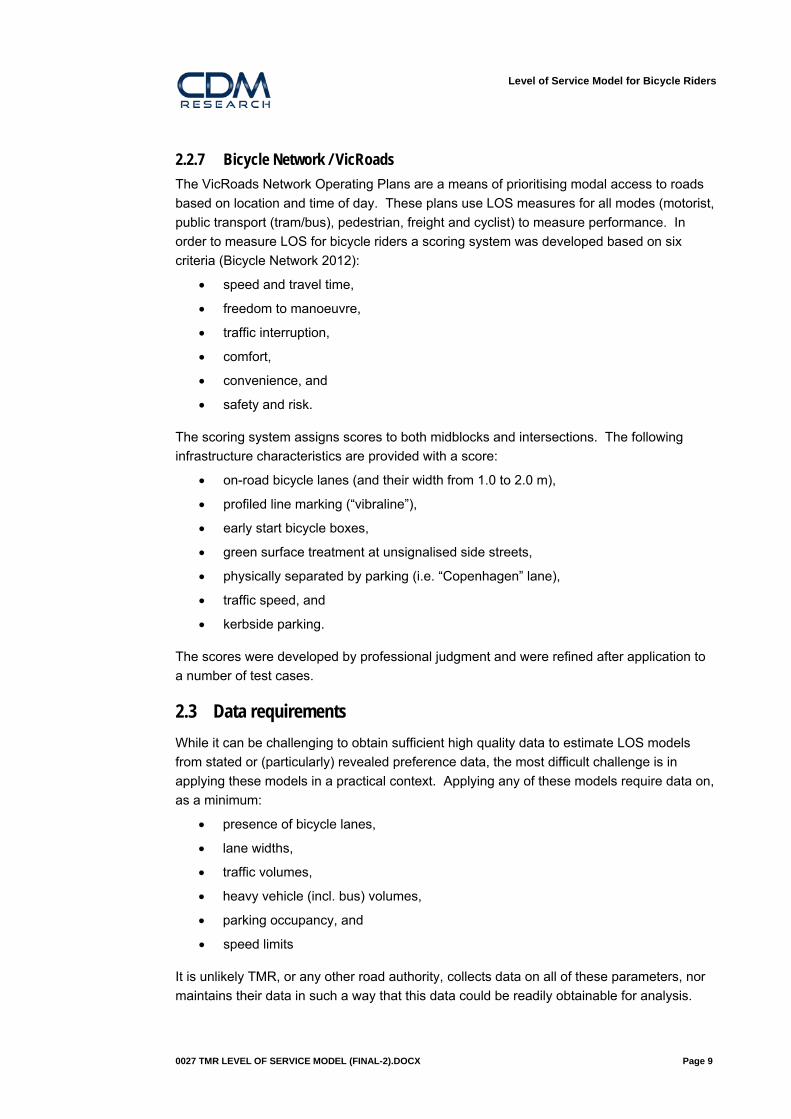
2.2.7 Bicycle Network / VicRoads
The VicRoads Network Operating Plans are a means of prioritising modal access to roads
based on location and time of day. These plans use LOS measures for all modes (motorist,
public transport (tram/bus), pedestrian, freight and cyclist) to measure performance. In
order to measure LOS for bicycle riders a scoring system was developed based on six
criteria (Bicycle Network 2012):
speed and travel time,
freedom to manoeuvre,
traffic interruption,
comfort,
convenience, and
safety and risk.
The scoring system assigns scores to both midblocks and intersections. The following
infrastructure characteristics are provided with a score:
on-road bicycle lanes (and their width from 1.0 to 2.0 m),
profiled line marking (“vibraline”),
early start bicycle boxes,
green surface treatment at unsignalised side streets,
physically separated by parking (i.e. “Copenhagen” lane),
traffic speed, and
kerbside parking.
The scores were developed by professional judgment and were refined after application to
a number of test cases.
2.3 Data requirements
While it can be challenging to obtain sufficient high quality data to estimate LOS models
from stated or (particularly) revealed preference data, the most difficult challenge is in
applying these models in a practical context. Applying any of these models require data on,
as a minimum:
presence of bicycle lanes,
lane widths,
traffic volumes,
heavy vehicle (incl. bus) volumes,
parking occupancy, and
speed limits
It is unlikely TMR, or any other road authority, collects data on all of these parameters, nor
maintains their data in such a way that this data could be readily obtainable for analysis.

Level of Service Model for Bicycle Riders
0027 TMR LEVEL OF SERVICE MODEL (FINAL-2).DOCX Page 10
The challenges of developing and then maintaining a database with this range of attributes
would be very time consuming and costly. While such data could readily be obtained on a
site-by-site basis, it would be difficult to obtain and maintain to a current status for large
areas. As such, it is likely that the practical deployment of any LOS model would be limited
to a well-defined corridor or area, and would require the collection of primary data within
that area.
2.4 Limitations of existing approaches
There are a number of limitations which apply to at least some of the existing LOS models:
The scores are based entirely on professional judgement, which may or may not
accord with the wider riding public (e.g. CERS, Bicycle Network/VicRoads),
The model coefficients are based on overseas conditions and riders, which may
differ markedly from Australian conditions (e.g. BLOS, BCI are both American and
the Danish BLOS model), and
Many of the models do not account for high quality separated on-road infrastructure
(i.e. “Copenhagen” lanes) which are the subject of significant policy interest.
2.5 Which model is ‘best’? Determining which model is best will, of course, depend on the application and the criteria
by which one wishes to measure “best”. In this section we provide some commentary on
this issue.
Widespread use and experience
The BLOS model is far more widely used in the USA than the BCI model. It is also based
on perceptions involving real cycling travel and videos from a cyclist’s perspective (rather
than stationary kerbside video in the case of the BCI model). This model forms the basis of
the LOS model within the most recent update of the Highway Capacity Manual (HCM), and
so has (presumably) been subject to a deal of scrutiny – and is now formally adopted within
the USA’s main traffic engineering manual. None of the other models appear to have been
adopted this widely, or formally, within their jurisdictions.
Reproducibility
Somenahalli (2008) applied the BCI and BLOS models to a section of Adelaide and found
no statistically significant difference between the models. However, the BLOS model was
somewhat more sensitive to higher vehicle volumes and speed. However, both models
were calibrated to US conditions – which may, or may not, be appropriate to Australia.
Model specification
The Danish model employs the most sophisticated model specification, and includes a
number of terms for segregated cycleways which are likely to be useful in an Australian
context. The use of a cumulative logit formulation allows for the use of the model in route
choice models.

Level of Service Model for Bicycle Riders
0027 TMR LEVEL OF SERVICE MODEL (FINAL-2).DOCX Page 11
Sampling and bias
Many of the models (including the model developed in this study) rely on a self-selected
sample of bicycle riders from the target population. This means there will be very little
sample control, and there is a real risk that sample will be skewed relative to the wider
riding population. In which way this skew may affect the results cannot be known with
certainty, but clearly this is a significant caveat to such methods. The only existing study
which appears to have used a genuine random, controlled sampling method was the
Danish model. However, the costs of recruitment and retention using this approach are
considerable.
Infrastructure types
Many of the models, and particularly those from North America, do not consider high quality
infrastructure such as physically protected bicycle lanes. This limitation has been noted
elsewhere, and would limit the application of these models in an Australian context where
these treatments are of interest.
Model transferability
In all likelihood if an existing LOS model were to be adopted for Queensland use the most
likely candidates would be some variation of the US BLOS or Danish BLOS. Two types of
tests would be required to determine which, if any, of these two models would be most
applicable:
1. Implement the models as-is for a test geography then compare the model
outcomes with one another and with expectation.
2. Sensitivity tests should then be undertaken to ensure the models respond in a
consistent and plausible manner. These sensitivity tests are very important – if the
LOS model is to be used to monitor and evaluate network improvements it must be
able to capture adequately such improvements. Sensitivity tests can be readily
undertaken in GIS and standard spatial regression methods used to evaluate any
changes.
The American studies are based on self-reported perceptions towards video and (in the
case of BLOS) riding different types of routes. These locations have very different road
infrastructure than Queensland (at least, compared with inner Brisbane) and are now at
least 14 years old. Furthermore, when the Danish model was compared with the US
models it would found to be more sensitive to the presence of cycling infrastructure. It was
hypothesised that this is because Danes are more familiar with such infrastructure than
most US cyclists, and so value it more highly. Given the current context in Brisbane (most
particularly the inner suburbs) this is likely to be important here also.
How could these models be improved?
There are at least two options for improving these models:

Level of Service Model for Bicycle Riders
0027 TMR LEVEL OF SERVICE MODEL (FINAL-2).DOCX Page 12
Develop and field a survey to determine local parameters, and expand to
incorporate other parameters of interest (e.g. segregated cycleways, impact of
cyclist/pedestrian volumes on LOS).
Calibrate the model using observed counts (permanent counters, Super Tuesday)
and observed route choices (Bicycle Victoria’s RiderLop iphone app).
The present study consists of the first of these options.

Level of Service Model for Bicycle Riders
0027 TMR LEVEL OF SERVICE MODEL (FINAL-2).DOCX Page 13
3 Methodology 3.1 Outline A detailed online survey asking riders to think in depth about their route choice preferences
was developed in order to quantify the different components of level of service. This survey
included the presentation of three stated preference (SP) experiments. The sampling
process was uncontrolled; respondents were invited to participate through online cycling
forums, email lists, social media and word of mouth. TMR staff were also invited to
participate through an internal staff email.
3.2 Online survey The online survey asked a range of questions about existing riding patterns and perceptions
towards bicycle facilities, including:
the respondent’s experience riding bicycles, how often they typically ride and for
what purposes,
information on their most recent riding trip (to use as a basis for the stated
preference experiments),
perceptions towards off-road shared paths and interactions with path users,
perceptions towards on-road riding and on-road bicycle facilities, and
demographic information.
The specific questions asked are provided as part of the discussion of the results in Section
4. In addition to these questions, the majority of the survey consisted of three stated
preference experiments. These are discussed in the following section.
3.3 Stated preference survey It has been widely established that riders have a preference for bicycle facilities, both from
observed counts of riders and from surveys. What is required for an LOS model is to
quantify these preferences in such a way that we can better understand the real-world
trade-offs that riders are prepared to make to use these types of facilities.
The approach adopted to quantify these route preferences was the use of stated preference
(SP) surveys. These surveys present a series of hypothetical choices to respondents and
ask them to choose their preferred option. This survey method is widely used in transport
modelling, and has the advantage that the research team can control the presentation of
the alternatives in a way that is not possible in the real-world. However, these methods
have a significant limitation in that they assume that the way respondents choose between
hypothetical alternatives on a survey would be the same as that in practice. This is a major
issue with these types of surveys, and is usually addressed by (a) trying to ensure the
scenarios are as realistic as possible (partly by basing them on a real trip the respondent
had recently undertaken), and (b) calibrating the models with revealed preference (real-

Level of Service Model for Bicycle Riders
0027 TMR LEVEL OF SERVICE MODEL (FINAL-2).DOCX Page 14
world) choice data. The former approach was taken in this study, and a discussion of the
latter approach is presented in Section 10.2.
In this survey, there were three SP experiments and eight scenarios within each experiment
was presented to respondents (giving a total of 24 choice sets per respondent). The
experiments were:
Off-road paths (Figure 3.1),
On-road facilities (Figure 3.2), and
Off-road vs on-road (Figure 3.3).
These three experiments, and the variables within the experiments, were designed to
present as simple but realistic choice sets as possible to respondents. Furthermore,
common variables of delay and travel time were used across all three experiments to allow
for joint estimation (as discussed in Section 5.3).
Figure 3.1: Off-road path SP experiment

Level of Service Model for Bicycle Riders
0027 TMR LEVEL OF SERVICE MODEL (FINAL-2).DOCX Page 15
Figure 3.2: On-road facilities SP experiment
Figure 3.3: On-road versus off-road SP experiment

Level of Service Model for Bicycle Riders
0027 TMR LEVEL OF SERVICE MODEL (FINAL-2).DOCX Page 16
The levels used in the experiments are given in Table 3.1. These levels were selected
based on a fractional factorial design, simulation and a final sense check (removal of
dominant designs) once the design was folded.
Table 3.1: Variable levels
Variable Experiment Levels
Travel
time
Off‐road 80% 90% Self‐
reported
trip time
110% 120%
On‐road 80% Self‐
reported
trip time
110% 130%
On‐ vs off‐
road
Self‐
reported
trip time
120% 140%
Overtake
pedestrian
Off‐road 3 mins 4 mins 7 mins 8 mins 10 mins 12 mins
Overtake
cyclist
Off‐road 3 mins 4 mins 7 mins 8 mins 10 mins 15 mins
Pass
someone
in other
direction
Off‐road 3 mins 4 mins 7 mins 8 mins 10 mins 15 mins
Delayed
by other
user
Off‐road,
on‐road, on‐
vs off‐road
3 mins 5 mins 8 mins 10 mins 15 mins
Facility On‐road,
on‐ vs off‐
road
Off‐road
path
(on‐ vs
off‐road
SP only)
No lane Bicycle
lane
Coloured
bicycle
lane
(only
SP3)
Protected
bicycle
lane
Traffic
speed
limit
On‐road,
on‐ vs off‐
road
50
km/h* 60 km/h 80 km/h
Traffic
volume
On‐road,
on‐ vs off‐
road
Light
(every 2
mins)
Moderate
(every 30
s)
Heavy
(every 5
s)

Level of Service Model for Bicycle Riders
0027 TMR LEVEL OF SERVICE MODEL (FINAL-2).DOCX Page 17
Variable Experiment Levels
Bus traffic On‐road Light
(every
20 mins)
Moderate
(every 10
mins)
Heavy
(every 2
min)
Kerbside
parking
On‐road No Yes
* Denotes base level in model estimation.

Level of Service Model for Bicycle Riders
0027 TMR LEVEL OF SERVICE MODEL (FINAL-2).DOCX Page 18
4 Survey results 4.1 Summary statistics A total of 729 respondents started the online survey, of which 439 (60%) completed the
survey. A further five respondents were removed who completed the survey in less than 15
minutes, leaving a total sample of 443 respondents for analysis.
The most frequently cited reference for finding out about the survey was through bicycle
user groups (36%), followed by TMR staff (30%) and through Bicycle Queensland (17%)
(Figure 4.1). 37% of respondents did not indicate where they had heard about the survey.
Figure 4.1: How did you hear about this survey?
Almost all respondents had most recently ridden in the past week (Figure 4.2). This result
is not surprising given the sampling method and likelihood that more active riders will be
more likely to respond than inactive riders.
45%
23%
10% 10% 9%
3%
BUG BicycleQueensland
Other socialmedia
Online bikeforum
TMR Cycling Qld
n = 271

Level of Service Model for Bicycle Riders
0027 TMR LEVEL OF SERVICE MODEL (FINAL-2).DOCX Page 19
Figure 4.2: When did you last ride a bicycle?
The sample consists of predominantly regular riders; 67% ride on at least four days in a
typical week and a further 25% at least twice a week (Figure 4.3).
Figure 4.3: How often do you ride a bicycle?
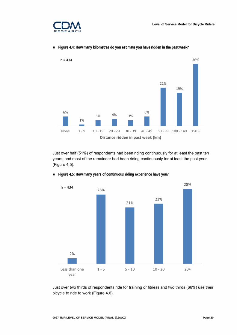
Just over a third (36%) of respondents had ridden more than 150 km in the past week, and
41% had ridden 50 to 150 km (Figure 4.4).
92%
6%2% 1%
Within the past week Within the past month Within the past sixmonths
Within the last year
n = 434
30%
37%
25%
3% 3%2%
Daily Four to fivedays a week
Two to threedays a week
Once a week Several times amonth
Several times ayear
n = 434
Level of Service Model for Bicycle Riders
0027 TMR LEVEL OF SERVICE MODEL (FINAL-2).DOCX Page 20
Figure 4.4: How many kilometres do you estimate you have ridden in the past week?
Just over half (51%) of respondents had been riding continuously for at least the past ten
years, and most of the remainder had been riding continuously for at least the past year
(Figure 4.5).
Figure 4.5: How many years of continuous riding experience have you?
Just over two thirds of respondents ride for training or fitness and two thirds (66%) use their
bicycle to ride to work (Figure 4.6).
6%
1%3% 4% 3%
6%
22%
19%
36%
None 1 ‐ 9 10 ‐ 19 20 ‐ 29 30 ‐ 39 40 ‐ 49 50 ‐ 99 100 ‐ 149 150 +
Distance ridden in past week (km)
n = 434
2%
26%
21%23%
28%
Less than oneyear
1 ‐ 5 5 ‐ 10 10 ‐ 20 20+
n = 434

Level of Service Model for Bicycle Riders
0027 TMR LEVEL OF SERVICE MODEL (FINAL-2).DOCX Page 21
Figure 4.6: Thinking about the times when you ride a bicycle, which of the following are applicable to you? (multi-response)
In order to classify respondents by their frequency and confidence riding bicycles a number
of questions were asked about their riding habits. This included asking respondents asking
respondents to classify themselves as “cautious” or “confident” when riding on-road. While
the frequency and types of riding undertaken by the sample would be suggestive of a
generally confident sample of riders, just under half (47%) indicated they were cautious
road riders and had a preference for paths or low stress roads (Figure 4.7). This
segmentation is used in the route choice models described in Section 5.
77%
67%
45%
29%
10%3%
I ride fortraining or
fitness, oftenriding longdistances
I ride to orfrom mywork
I ride forenjoyment,often alongquiet streetsor through
parks
I ride aroundmy local areato do myshopping,meetig upwith friends
etc
I ride as away ofgettingbetween
places whichI'm working
I ride to orfrom the
place where Istudy (school,university,TAFE)
n = 434

Level of Service Model for Bicycle Riders
0027 TMR LEVEL OF SERVICE MODEL (FINAL-2).DOCX Page 22
Figure 4.7: We would like you to think about the way you ride your bike in the presence of traffic when on-road. Which of the following do you feel best describes your riding style?
4.2 Trip context It is likely that route preferences will vary by the purpose of journey (as well as on individual
characteristics). To provide context to the route choice questions respondents were asked
to think about their most recent cycling trip. Just under half (45%) of respondents had most
recently ridden for commuting, followed by training/fitness (35%) and for recreation (14%)
(Figure 4.8).
Figure 4.8: Now we would like you to think about the most recent trip you made by bicycle. Which of the following best describes the purpose of your trip?
47%
53%
Cautious (prefer paths or low stress roads andwilling to take a longer route to get to a
destination)
Confident (prefer to use the most direct andconvenient route, regardless of traffic
conditions)
n = 434
45%
35%
14%
2% 1%3%
n = 434

Level of Service Model for Bicycle Riders
0027 TMR LEVEL OF SERVICE MODEL (FINAL-2).DOCX Page 23
Once very short (less than 5 minutes) and very long (more than 6 hours) trips are removed
the average trip duration was 69 minutes (Table 4.1).
Table 4.1: Most recent trip duration statistics
No. of observations 414
Minimum 5 mins
Maximum 6 hrs
Average 69 mins
Median 60 mins
Standard deviation 70 mins
Most respondents had ridden a road bike (54%), followed by mountain bikes (22%) (Figure
4.9).
Figure 4.9: What sort of bicycle did you ride?
Respondents were asked whether they changed clothes at their destination (to serve as a
proxy for “effort”); 70% had a shower and got changed while 16% continued to wear the
same clothes (Figure 4.10). The proportion who had a shower increased with riding time,
as would be expected. Around 70% of those who rode for over 30 minutes had a shower
afterwards, compared to 57% of those who rode for 30 minutes or less (and 50% of those
who rode for 15 minutes or less).
54%
22%19%
1% 1% 0%3%
Road bike Mountainbike
Flat barroad bike
City bike Recumbent Foldingbike
Other
n = 434

Level of Service Model for Bicycle Riders
0027 TMR LEVEL OF SERVICE MODEL (FINAL-2).DOCX Page 24
Figure 4.10: When you arrived at your destination did you…?
Two thirds of respondents had ridden alone (Figure 4.11), suggesting their route choice
preferences were theirs alone. For the remainder, who rode in groups, presumably the
choice of route was determined communally.
Figure 4.11: Were you riding alone?
Respondents indicated that on average they spent around 49% of their journey on-road with
no bicycle facility, 21% on off-road paths and 18% on on-road bicycle lanes (Figure 4.12).
70%
16%
10%
4%
Have a shower and getchanged
Continue to wear the sameclothes
Get changed Other
n = 434
65%
34%
1%
Ride alone Ride with other adult(s) Ride with kid(s)
n = 429

Level of Service Model for Bicycle Riders
0027 TMR LEVEL OF SERVICE MODEL (FINAL-2).DOCX Page 25
Unsurprisingly, those cyclists who indicated they were confident road riders (Figure 4.7)
rode a larger proportion of their trip on-road without facilities (58% of their travel time,
compared with40% of cautious riders).
Figure 4.12: How much time did you spend on these types of routes?
4.3 Route choices The survey asked respondents to rate (e.g. rate from “very uncomfortable” to “very
comfortable”) and rank (i.e. order a number of options from most to least preferred) their
preferences to particular attributes of off-road paths and on-road conditions for cycling.
These ratings and rankings for different types of facilities and conditions are discussed in
this section.
4.3.1 Off-road paths
Respondents were asked to rate attributes of shared paths such as surface quality, lighting
and the presence of other path users. The results, shown in Figure 4.13, ordered by the
proportion indicating “very uncomfortable” suggests that people with dogs, children, lots of
intersections and blind corners are the variables which make riders most uncomfortable on
paths. Conversely, nice scenery, a low number of cyclists and separation from pedestrians
were the most desirable path attributes.
40%
58%
49%
16%
20%
18%
29%
13%
21%
16%
8%
12%
Cautious
Confident
All
On‐road, no facility
On‐road bicycle lane
Off‐road path
Cycleway
n = 434

Level of Service Model for Bicycle Riders
0027 TMR LEVEL OF SERVICE MODEL (FINAL-2).DOCX Page 26
Figure 4.13: When riding on a shared path for <purpose>, how comfortable do you feel in each of the following?
Another approach which produced similar results was to ask respondents to rank the
attributes from most to least preferred. This ranking is shown in Figure 4.14, ordered based
on the least preferred ranking. The most onerous interactions are similar in both the rating
and ranking questions; interactions with unpredictable users (pedestrians with dogs and
children).
Figure 4.14: Listed below are some typical interactions on a shared path. Please rank these interactions in order from most preferred (1) to least preferred (10).
31%
27%
23%
14%
14%
4%
3%
3%
40%
41%
42%
49%
47%
26%
19%
6%
9%
6%
5%
16%
19%
17%
18%
23%
21%
24%
22%
18%
9%
7%
8%
6%
12%
20%
11%
10%
13%
15%
12%
34%
36%
42%
47%
34%
33%
26%
23%
34%
27%
6%
4%
5%
15%
18%
28%
24%
50%
54%
65%
70%
53%
53%
0% 10% 20% 30% 40% 50% 60% 70% 80% 90% 100%
Pedestrians with dogs
Children
Lots of intersections
Blind corners
Overhanging branches
Narrow path
Fence or wall next to path
Good lighting
Steep hills
Low no. of pedestrians
Able to ride at any speed
Smooth surface
Separation from pedestrians
Low no. of cyclists
Nice scenery
Very uncomfortable Uncomfortable Neutral Comfortable Very comfortable n = 434
0% 20% 40% 60% 80% 100%
Passing a pedestrian with a dog
Pass a young child on a bike
Overtaking two pedestrians walking side by side
Overtaking another user, but having to slow because you can't getpast straight away
Overtaking a pedestrian
Being overtaken by another cyclist
Passing a pedestrian walking in the opposite direction
Passing another cyclist riding in the opposite direction
Overtaking another cyclist
1 ‐ Most preferred
2
3
4
5
6
7
8
9 ‐ Least preferred
n = 429

Level of Service Model for Bicycle Riders
0027 TMR LEVEL OF SERVICE MODEL (FINAL-2).DOCX Page 27
Respondents were presented with four sets of physical characteristics of paths as shown in
Figure 4.15. The segregated facility was highly approved of (55% of respondents), while
the shared path received a more mixed reception (although only 23% disliked riding on
such a facility). The presence of vegetation and walls that reduce the effective path width
were both seen as discomforting.
Figure 4.15: In this question we are interested in how the physical characteristics of a path influence your comfort when you are riding for <purpose>. How would you feel riding on these paths?
Path with cyclists and
pedestrians segregated
Path shared with pedestrians
and cyclists
Path shared with pedestrians
and cyclists with vegetation
overgrowing on the edge
Path shared with pedestrians
and cyclists with a wall on one
side
4.4 Delayed passing Respondents were then presented with a series of five short (< 20 second) video clips
illustrating various interactions that may occur with other path users. Respondents were
asked to rate these interactions from one (doesn’t bother me at all) to five (bothers me a
lot). The results, ordered by the proportion indicating “doesn’t bother me at all” is shown in
Figure 4.163. These videos served the dual purpose of introducing the different types of
interaction (which are difficult to describe in words or with diagrams or pictures) as well as
providing information on preferences towards these interactions.
3 Around 15% of respondents could not view the YouTube clips on their computer and so were not presented with these questions. It is common to block YouTube access in corporate environments.
3%
10%
9%
20%
29%
35%
5%
37%
37%
30%
37%
35%
21%
22%
55%
5%
3%
3%
0% 10% 20% 30% 40% 50% 60% 70% 80% 90% 100%
Segregated
Shared path
Shared path with wall on one side
Shared path with vegetation overgrowing edge of path
Really dislike Dislike Neither like nor dislike Like Really like
n = 434

Level of Service Model for Bicycle Riders
0027 TMR LEVEL OF SERVICE MODEL (FINAL-2).DOCX Page 28
The results suggest that riders perceive delays as the most bothersome, followed by
overtaking pedestrians travelling in the same direction. These results appear reasonable
given that most riders were travelling for transport (so are presumably time sensitive) and
overtaking someone travelling in the same direction is more complex than someone
travelling in the opposite direction (where both users can see one another). Furthermore, it
is consistent with the results reported above that riders feel more discomforted passing
other pedestrians than other riders.
Figure 4.16: When riding on a shared path you may experience a number of different interactions with other people. We would like you to look at the following short video clips and rate how you feel about each of these interactions…
Respondents were then asked to rate the regularity of being delayed by interactions with
other path users. The regularity with which a rider is delayed was hypothesised to be an
important consideration in a cyclists’ perception of convenience, particularly for transport
trips. However, it is difficult to directly relate to the regularity of delay and to identify at what
regularity it becomes unduly onerous. To partially redress this issue respondents were
asked about their perception towards delay in different ways. While somewhat repetitive for
respondents, by approaching the problem in different ways greater confidence can be
garnered from the result, and the importance of the survey method in influencing the result
can be better understood.
Delay was expressed as a headway – e.g. delayed every 5 minutes, as earlier pilot testing
indicated this was easier for respondents to understand than a frequency (e.g. 12 delays
per hour). Firstly, respondents were asked to rate their tolerance towards delay across six
delay headways (presented from least frequent to most frequent). This question type is
often referred to as a stated intention (SI). As shown in Figure 4.17, for most individuals
delays every 15 minutes or less often were not considered bothersome. Conversely, delays
every minute were considered as very bothersome by 62% of respondents.
82%
69%
60%
54%
26%
15%
22%
20%
27%
21%
7%
10%
11%
20%
7%
23% 10%
0% 20% 40% 60% 80% 100%
Meet a cyclist travelling in the oppositedirection
Overtake a cyclist travelling in the samedirection
Pass a pedestrian travelling in the oppositedirection
Overtake a pedestrian travelling in the samedirection
Being delayed by other people
1 ‐ Doesn't bother me at all
2
3
4
5 ‐ Bothers me a lot
n = 366

Level of Service Model for Bicycle Riders
0027 TMR LEVEL OF SERVICE MODEL (FINAL-2).DOCX Page 29
Figure 4.17: We would now like you to think a little further about how being delayed by other people affects your comfort on shared paths. Think about when you are riding for <purpose>, how would you rate a path where you have to give way before overtaking once every…
Secondly, respondents were asked directly to indicate at what headway they would be
“bothered a little” and “bothered a lot” – i.e. they were asked to enter a number of their
choice. This type of question is a contingent valuation question.
It is implausible that a respondent would report a lower headway for being bothered a little
compared with bothered a lot. For example, if a respondent indicated that being delayed
once every 10 minutes bothered them a little then we would expect being delayed at some
headway smaller than 10 minutes would bother them a lot. Checks were performed on the
data to ensure this was the case; in 67 instances (15%) this was not the case and so these
respondents were not considered in this section (as we conclude they had misunderstood
the question). Once these cases were excluded the average delay headway to be bothered
a little was 11.0 minutes and to be bothered a lot was 4.1 minutes (Table 4.2).
Table 4.2: We would like you to think a little more about how often you wold be prepared to be delayed by other people. Please think about when you are riding for an <purpose> trip. How often would you be prepared to be delayed by other people before it…?
Bothered you a little Bothered you a lot
n 367
Average 11.0 mins 4.1 mins
Median 10.0 mins 3.0 mins
Standard Dev. 10.0 mins 4.1 mins
7%
6%
16%
35%
50%
66%
5%
10%
15%
21%
23%
15%
9%
18%
25%
19%
12%
7%
18%
25%
23%
15%
6%
2%
62%
41%
21%
11%
9%
10%
0% 20% 40% 60% 80% 100%
1 min
3 min
5 min
10 min
15 min
20 min
1 ‐ Doesn't bother me at all
2
3
4
5 ‐ Bothers me a lot
n = 434
Level of Service Model for Bicycle Riders
0027 TMR LEVEL OF SERVICE MODEL (FINAL-2).DOCX Page 30
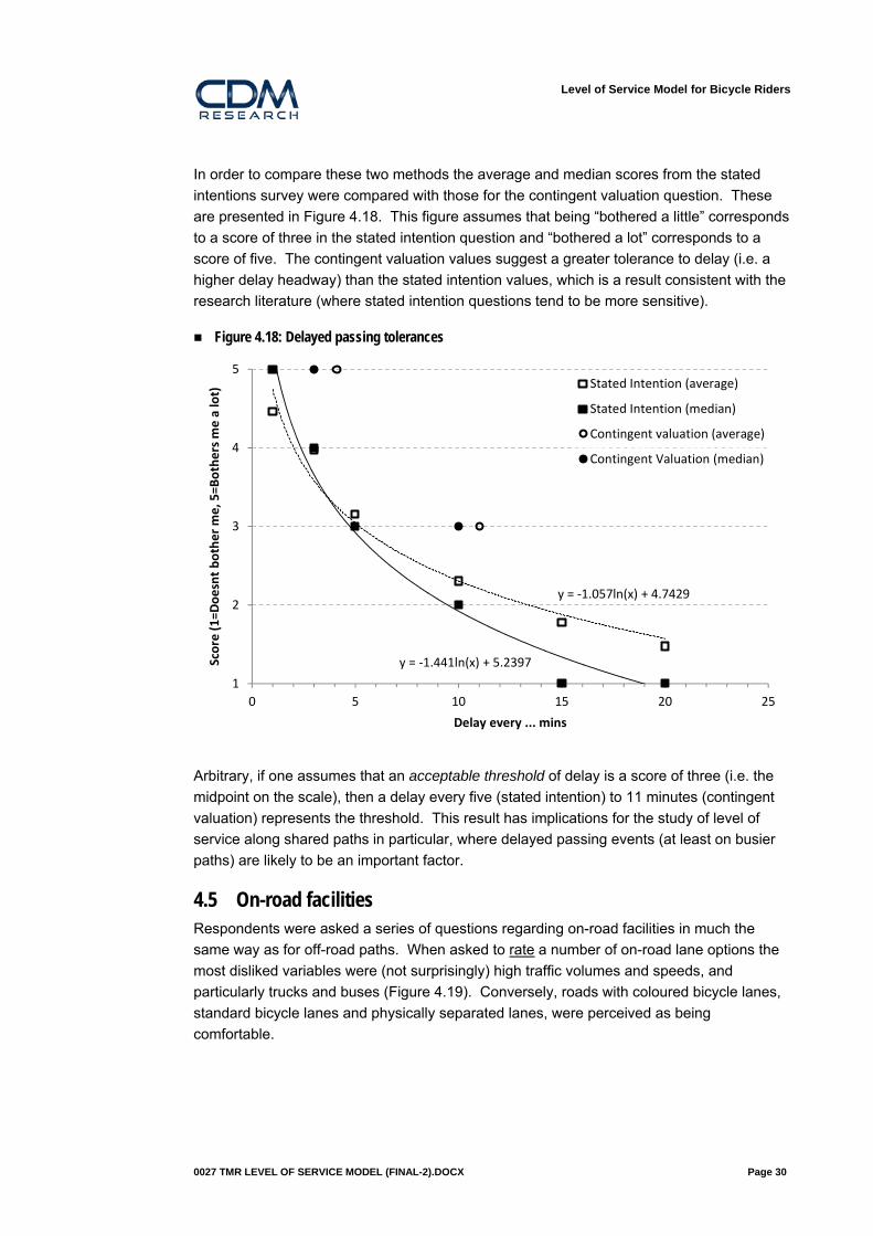
In order to compare these two methods the average and median scores from the stated
intentions survey were compared with those for the contingent valuation question. These
are presented in Figure 4.18. This figure assumes that being “bothered a little” corresponds
to a score of three in the stated intention question and “bothered a lot” corresponds to a
score of five. The contingent valuation values suggest a greater tolerance to delay (i.e. a
higher delay headway) than the stated intention values, which is a result consistent with the
research literature (where stated intention questions tend to be more sensitive).
Figure 4.18: Delayed passing tolerances
Arbitrary, if one assumes that an acceptable threshold of delay is a score of three (i.e. the
midpoint on the scale), then a delay every five (stated intention) to 11 minutes (contingent
valuation) represents the threshold. This result has implications for the study of level of
service along shared paths in particular, where delayed passing events (at least on busier
paths) are likely to be an important factor.
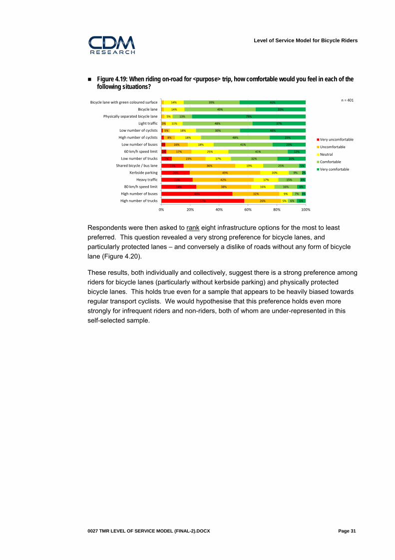
4.5 On-road facilities Respondents were asked a series of questions regarding on-road facilities in much the
same way as for off-road paths. When asked to rate a number of on-road lane options the
most disliked variables were (not surprisingly) high traffic volumes and speeds, and
particularly trucks and buses (Figure 4.19). Conversely, roads with coloured bicycle lanes,
standard bicycle lanes and physically separated lanes, were perceived as being
comfortable.
y = ‐1.057ln(x) + 4.7429
y = ‐1.441ln(x) + 5.2397
1
2
3
4
5
0 5 10 15 20 25
Score (1=D
oesnt bother me, 5=B
others m
e a lot)
Delay every ... mins
Stated Intention (average)
Stated Intention (median)
Contingent valuation (average)
Contingent Valuation (median)
Level of Service Model for Bicycle Riders
0027 TMR LEVEL OF SERVICE MODEL (FINAL-2).DOCX Page 31
Figure 4.19: When riding on-road for <purpose> trip, how comfortable would you feel in each of the following situations?
Respondents were then asked to rank eight infrastructure options for the most to least
preferred. This question revealed a very strong preference for bicycle lanes, and
particularly protected lanes – and conversely a dislike of roads without any form of bicycle
lane (Figure 4.20).
These results, both individually and collectively, suggest there is a strong preference among
riders for bicycle lanes (particularly without kerbside parking) and physically protected
bicycle lanes. This holds true even for a sample that appears to be heavily biased towards
regular transport cyclists. We would hypothesise that this preference holds even more
strongly for infrequent riders and non-riders, both of whom are under-represented in this
self-selected sample.
57%
49%
24%
22%
20%
15%
7%
3%
3%
26%
32%
38%
42%
49%
36%
23%
17%
16%
8%
5%
3%
5%
9%
16%
17%
20%
19%
17%
25%
18%
18%
18%
11%
5%
14%
14%
6%
7%
16%
15%
9%
25%
32%
41%
41%
48%
30%
48%
13%
49%
39%
6%
3%
6%
4%
2%
5%
20%
12%
23%
25%
46%
37%
79%
35%
46%
0% 20% 40% 60% 80% 100%
High number of trucks
High number of buses
80 km/h speed limit
Heavy traffic
Kerbside parking
Shared bicycle / bus lane
Low number of trucks
60 km/h speed limit
Low number of buses
High number of cyclists
Low number of cyclists
Light traffic
Physically separated bicycle lane
Bicycle lane
Bicycle lane with green coloured surface
Very uncomfortable
Uncomfortable
Neutral
Comfortable
Very comfortable
n = 401

Level of Service Model for Bicycle Riders
0027 TMR LEVEL OF SERVICE MODEL (FINAL-2).DOCX Page 32
Figure 4.20: We’d like you to think in general about roads with moderate to high volumes of traffic. Please rank the following situations from 1 (most preferred) to 8 (least preferred) on these types of roads.
No bike lane, no parking Wide shoulder, no parking No bike lane, adjacent parking Bike lane, no parking
Bike lane, adjacent parking Green bike lane, no parking Physically separated bike lane Protected bike lane
0% 20% 40% 60% 80% 100%
No bike lane, adjacent parking
Bike lane, adjacent parking
Shared bus/bike lane
No bike lane, no parking
Painted bike lane, adjacent parking
Protected bicycle lane
Bike lane
1 ‐ Most preferred
2
3
4
5
6
7 ‐ Least preferred
n = 434

Level of Service Model for Bicycle Riders
0027 TMR LEVEL OF SERVICE MODEL (FINAL-2).DOCX Page 33
5 Discrete choice model 5.1 Outline This section describes the estimation of LOS models from the stated preference survey
data. A non-mathematical background on the model structure is presented, as well as the
model results and interpretation.
5.2 Discrete choice models Discrete choice models are used where respondents are choosing from a discrete range of
options (e.g. to use route A or route B). These models are often based on multinomial logit
models. These logit models can be thought of as an extension of classical regression
analysis to categorical (rather than continuous) variables. The most important characteristic
to note with these models is that they are probabilistic rather than deterministic. If there are
two route options A and B, the logit model assigns a probability of selection to each of the
two alternatives. For example, if A is more attractive than B it may have a probability of 0.7.
This indicates that we expect there to be a 70% chance of an individual selecting route A.
To think of this another way, if there were 100 riders choosing between the routes we would
expect 70 to choose route A. This probabilistic approach tends to produce more realistic
forecasts than deterministic approaches (which would allocate all riders to the preferred
route), because of the unobserved attributes of the routes (i.e. those attributes which were
not modelled) and variation in the taste preferences between individuals.
5.3 Model estimation Model estimation is a statistical procedure whereby a specified model (on equation) is fit to
a set of data. In its’ simplest form this procedure is applied to fit linear models to a single
independent variable and single dependent variable (e.g. y = βx where β is estimated by
linear regression). As we have multiple variables, and a number are categorical, a logit
model is used with the stated preference data. These models tend to be more complex to
estimate and interpret than simple linear regressions, but have the same basic structure
(that is, they consist of an independent variable and one or more dependent variables, at
least one of which is categorical).
The SP experiments were setup in such a way that they had two common parameters
across all three experiments (delay and travel time). This allowed for the datasets from
each experiment to be pooled and jointly estimated using structural parameters (denoted by
θ) to account for the different error scales within each dataset4. This method is commonly
used within complex discrete choice modelling and allows a more complete model
specification to be tested without overwhelming respondents with overly complex choice
sets. The model structure is shown in Figure 5.1.
4 The scales are relative to the off-road experiment, so θoff‐road
is equal to one.

Level of Service Model for Bicycle Riders
0027 TMR LEVEL OF SERVICE MODEL (FINAL-2).DOCX Page 34
Figure 5.1: Joint estimation model structure
Each of the model coefficients are described in Table 5.1.
Table 5.1: Model coefficient descriptions
Parameters Unit Description
Structural parameters
ϴonroad none Error scale of on‐road SP relative to off‐road SP
(values < 1 imply greater unexplained variance)
ϴfacility none Error scale of facility SP relative to off‐road SP
(values < 1 imply greater unexplained variance)
User interactions
pedover events/min Number of pedestrian overtaking events per minute
(e.g. overtake 2 pedestrians per minute)
pass events/min Number of cyclist and pedestrian passing/meeting
events per minute (e.g. meet 4 path users coming
the other way per minute)
ln(delay) ln(events/min+1) Natural logarithm of the number of delayed passing
events per minute plus one (e.g. delayed by other
path users on average 0.5 times per minute – or
once every two minutes). The +1 was used to
ensure that events/min<1 had the same sign after
the logarithm was applied as those >1.
buspass events/mins Number of bus overtaking events per minute in the
nearside traffic lane

Level of Service Model for Bicycle Riders
0027 TMR LEVEL OF SERVICE MODEL (FINAL-2).DOCX Page 35
Parameters Unit Description
carpass events/mins Number of car overtaking events per minute in the
nearside traffic lane
Facility characteristics
park mins Additional (dis)utility per travel time minute due to
kerbside parking (relative to no kerbside parking)
speed60 mins Additional (dis)utility per travel time minute of 60
km/h speed limit (relative to 50 km/h speed limit)
speed80 mins Additional (dis)utility per travel time minute of 80
km/h speed limit (relative to 50 km/h speed limit)
time(path) mins Travel time on off‐road shared path
time(no lane) mins Travel time on‐road without bicycle facilities
time(lane) mins Travel time on‐road with bicycle lane
time(protected lane) mins Travel time on‐road with protected bicycle lane
(‘Copenhagen’ lane)
A large number of models were tested for statistical significance, and were estimated using
BIOGEME 2.25. Respondents who always selected option A, or always selected option B,
within an SP experiment were classed as non-traders and removed from the dataset. This
was found to improve the model fit (as measured by the t-values).
5.4 Dataset The model results presented in this section are for a pooled dataset, incorporating both the
Queensland survey results and an essentially identical survey conducted in Victoria in
2012. Separate model runs for each state suggested there was no meaningful difference
between the samples, and by pooling the data the statistical significance of the estimates
improved markedly.
5.5 Results Three models are presented in this section. These models correspond to the full sample of
respondents (all riders), confident riders and cautious riders (as self-reported by
respondents). The model coefficients and their t-ratios are presented in Table 5.2. The t-
ratios are the coefficient divided by the standard error; values of greater than 1.96 indicate
the coefficient is statistically significant at the 5% level. It is usual practice to retain
variables in the models that have t-ratios greater than 1.96.
The following simplifications were made to the full model specification:
5 http://biogeme.epfl.ch/

Level of Service Model for Bicycle Riders
0027 TMR LEVEL OF SERVICE MODEL (FINAL-2).DOCX Page 36
In all models travel time on green coloured bicycle lanes was insignificant. As such,
it was combined with the protected bicycle lane parameter; this had no material
impact on this parameter as the number of scenarios where green bicycle lanes
were presented was low.
In all models cyclist overtaking events were statistically insignificant – the models
do not incorporate this event.
The speed60 parameter was insignificant for the confident riders model, and so was
removed.
The time on protected bicycle lane parameter was marginally positive and
statistically insignificant for cautious riders. A positive time coefficient indicates a
positive utility (or preference) for additional travel time. This is contrary to economic
theory, where travel time is assumed to have a disutility (that is, travellers seek to
minimise their travel time). It is possible that, at least for recreational trips, riders do
indeed have a positive preference for travel on high quality lanes. Moreover, it
seems plausible that cautious riders would assign very high preferences for
physically segregated on-road provision (which in turn would imply a small time
parameter). Subsequent sensitivity tests suggested the retention of this parameter
marginally improved the plausibility of the model, and so it was retained. However,
the insignificance of this parameter means forecasts for protected bicycle lanes with
cautious riders should be treated with caution.

Level of Service Model for Bicycle Riders
0027 TMR LEVEL OF SERVICE MODEL (FINAL-2).DOCX Page 37
Table 5.2: Route choice models (Queensland and Victorian data)
All riders Confident riders Cautious riders
No. of observations 13,120 6,633 6,259
Final Log Likelihood ‐7,071.5 ‐3,610.3 ‐3,226.8
Degrees of Freedom 15 14 14
Adjusted ρ2 0.221 0.212 0.253
Parameter Estimate t‐ratio Estimate t‐ratio Estimate t‐ratio
Structural parameters
Onroad SP (ϴonroad) 0.668 13.24 0.635 9.97 0.673 8.43
Facility SP (ϴfacility) 0.438 11.84 0.694 8.80 0.364 8.30
User interactions
pedover ‐0.0493 ‐8.77 ‐0.0550 ‐6.76 ‐0.0437 ‐5.40
pass ‐0.0231 ‐4.77 ‐0.0222 ‐3.18 ‐0.0280 ‐3.94
delay ‐0.0800 ‐15.13 ‐0.0722 ‐10.19 ‐0.0891 ‐11.03
buspass ‐0.0464 ‐7.34 ‐0.0558 ‐6.75 ‐0.0635 ‐5.68
carpass ‐0.0027 ‐10.86 ‐0.0021 ‐7.34 ‐0.0037 ‐5.68
Facility characteristics
park (1) ‐0.0266 ‐8.17 ‐0.0125 ‐3.77 ‐0.0351 ‐6.21
speed60 (2) ‐0.0155 ‐6.77 n/a ‐0.0261 ‐6.64
speed80 (2) ‐0.0318 ‐10.61 ‐0.0197 ‐6.57 ‐0.0458 ‐8.07
time(path) ‐0.0528 ‐13.79 ‐0.0621 ‐11.47 ‐0.0417 ‐7.42
time(no lane) ‐0.0628 ‐12.20 ‐0.069 ‐10.70 ‐0.0696 ‐7.69
time(lane) ‐0.0175 ‐4.28 ‐0.0307 ‐5.72 ‐0.0142 ‐2.29
time(protected lane) 0.0253 4.70 ‐0.00635 ‐1.06 0.0501 5.52
(1) Relative to no kerbside parking (2) Relative to 50 km/h.
Values in italics are insignificant at the 5% level.
The model summary statistics are described in Table 5.3.
Level of Service Model for Bicycle Riders
0027 TMR LEVEL OF SERVICE MODEL (FINAL-2).DOCX Page 38
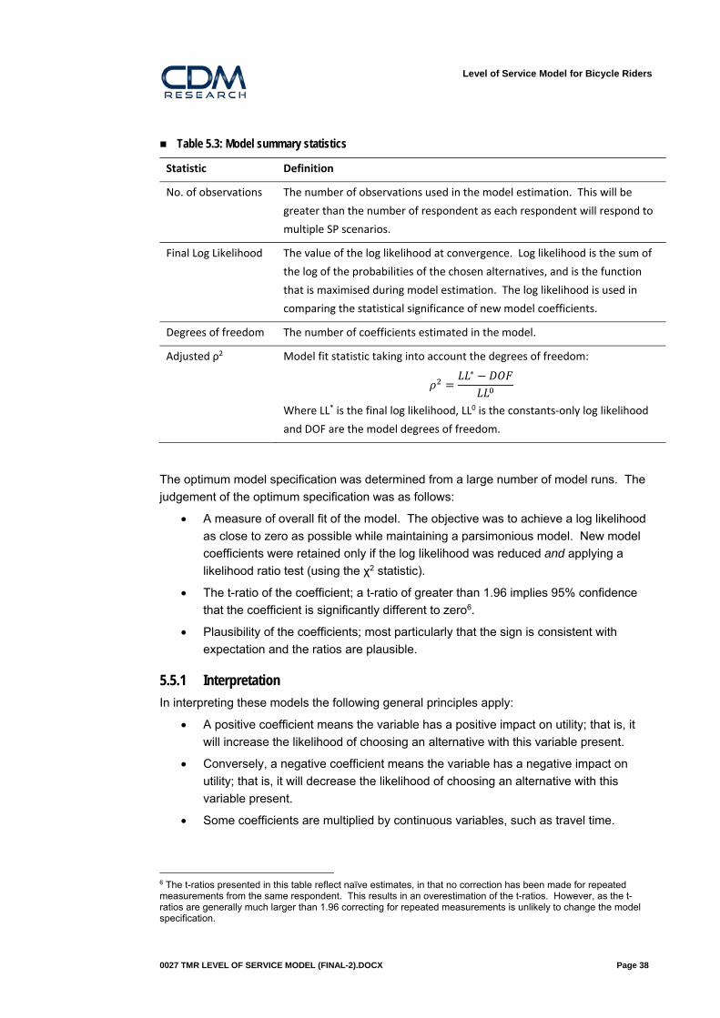
Table 5.3: Model summary statistics
Statistic Definition
No. of observations The number of observations used in the model estimation. This will be
greater than the number of respondent as each respondent will respond to
multiple SP scenarios.
Final Log Likelihood The value of the log likelihood at convergence. Log likelihood is the sum of
the log of the probabilities of the chosen alternatives, and is the function
that is maximised during model estimation. The log likelihood is used in
comparing the statistical significance of new model coefficients.
Degrees of freedom The number of coefficients estimated in the model.
Adjusted ρ2 Model fit statistic taking into account the degrees of freedom:
∗
Where LL* is the final log likelihood, LL0 is the constants‐only log likelihood
and DOF are the model degrees of freedom.
The optimum model specification was determined from a large number of model runs. The
judgement of the optimum specification was as follows:
A measure of overall fit of the model. The objective was to achieve a log likelihood
as close to zero as possible while maintaining a parsimonious model. New model
coefficients were retained only if the log likelihood was reduced and applying a
likelihood ratio test (using the χ2 statistic).
The t-ratio of the coefficient; a t-ratio of greater than 1.96 implies 95% confidence
that the coefficient is significantly different to zero6.
Plausibility of the coefficients; most particularly that the sign is consistent with
expectation and the ratios are plausible.
5.5.1 Interpretation
In interpreting these models the following general principles apply:
A positive coefficient means the variable has a positive impact on utility; that is, it
will increase the likelihood of choosing an alternative with this variable present.
Conversely, a negative coefficient means the variable has a negative impact on
utility; that is, it will decrease the likelihood of choosing an alternative with this
variable present.
Some coefficients are multiplied by continuous variables, such as travel time.
6 The t-ratios presented in this table reflect naïve estimates, in that no correction has been made for repeated measurements from the same respondent. This results in an overestimation of the t-ratios. However, as the t-ratios are generally much larger than 1.96 correcting for repeated measurements is unlikely to change the model specification.

Level of Service Model for Bicycle Riders
0027 TMR LEVEL OF SERVICE MODEL (FINAL-2).DOCX Page 39
Other coefficients are categorical variables, but have been scaled to travel time
units and are additive to the base condition. The speed60 and speed80 coefficients
are this type of variable; they represent an additional disutility per travel time minute
relative to 50 km/h roads. The park coefficient is the other coefficient of this type; if
kerbside parking is present there is an additional disutility per travel time minute
relative to an equivalent road without kerbside parking.
The models presented in Table 5.2 appear to be behaviourally plausible, as well as being
statistically significant. We discuss the meaning of these model coefficients in the following
sections.
Structural parameters
The structural parameters account for the different scales of the three different SP
experiments. The off-road path experiment is arbitrarily assigned as the base scale (i.e.
ϴoff-road = 1), for all models the scales of the on-road and facility SPs are significantly less
than one. This implies that the unexplained variance in the on-road and facility SPs is
greater than in the off-road SP. This is an expected result, as in some regards the off-road
SP is the simplest of the SP experiments, and is presented first (so likely to have more
attention paid to it by respondents)7.
User interactions
The user interaction terms are related to the frequency with which a rider may have to pass
or meet other path or road users, and may be delayed (either by other road or path users,
or by traffic signals). The unit of measurement in all cases is the number of events per
minute8. The interpretation of these coefficients is complicated by the transformations
applied to the delay parameter, however the following observations can be made:
pedover and pass are all linear parameters with negative signs, indicating that as
the frequency of these events increases so too does the disutility of that route. This
is the expected behaviour; we would expect very busy paths to be perceived less
favourably than quieter paths. Furthermore, pedover is about twice the magnitude
of pass. This suggests, plausibly, that pedestrian overtaking events are more
onerous than meeting events.
Delay has a negative sign, indicating that as the frequency of these events
increases so too does the disutility of that route. This is the expected behaviour.
Furthermore, delay is about 30% to 100% greater than pedover (and larger again
relative to pass). This indicates that delayed passing events are much more
onerous than pedestrian overtaking events that do not result in a delay (and
meeting events).
7 Conversely, it could be argued that as this SP is presented first the variance could be higher as respondents are still ‘learning’ how the trade-offs work. Our feeling is that this argument is not compelling. 8 This unit of measure makes the parameters independent of travel time. However, it does complicate model interpretation and parameter transformations because it can take positive values less than one (e.g. one event every two minutes would be 0.5 events/min).

Level of Service Model for Bicycle Riders
0027 TMR LEVEL OF SERVICE MODEL (FINAL-2).DOCX Page 40
The ratio between buspass and carpass events seems plausible; a bus passing
event has a disutility 17 to 27 times greater than a car passing event. In other
words, a bus overtaking event is perceived similarly to 17 to 27 cars overtaking.
Facility characteristics
The facility characteristic terms capture the infrastructure-specific characteristics of each
route alternative. The interpretation of these coefficients are as follows:
The park coefficient represents the additional (dis)utility of riding along a road with
kerbside parking compared to a road without kerbside parking. The coefficient is
negative, suggesting that riders prefer roads without kerbside parking. This
coefficient increases the travel time disutility on roads without bicycle lanes by 42%
for the all riders model. Interestingly, the additional disutility is greater for cautious
riders (an additional 50%) than for confident riders (18%).
speed60 and speed80 are both measured relative to a 50 km/h speed limit. Both
have a negative sign, indicating that roads with higher speed limits have a higher
disutility. That riders would feel less comfortable on higher speed roads is
consistent with our expectation. Furthermore, for the confident riders model the
speed60 term is insignificant, suggesting these riders do not perceive a difference
between roads at 50 and 60 km/h.
The speed60 and speed80 coefficients are measured in travel time units. As such,
they can be directly compared to the travel time coefficients. For the all riders
model a 60 km/h speed limit adds 25% to the travel time disutility (relative to a 50
km/h road), and an 80 km/h speed limit adds 51% to the travel time disutility. For
cautious riders the disutility is much greater – an additional 38% disutility for 60
km/h roads and 66% for 80 km/h roads.
The travel time coefficients are all negative (except for protected lanes for cautious
riders), implying that riders will be seeking to minimise their travel time (consistent
with other transport trips). The disutility of travel time reduces markedly when
bicycle facilities are provided on-road; the travel time disutility with bicycle lanes is
only 28% of a road without bicycles for all riders. Cautious riders assign greater
less disutility to bicycle lanes relative to no lanes (20%) than do confident riders
(44%), as we would expect. The reduction in disutility for the protected bicycle
lanes are even more marked, suggesting a very strong preference from riders for
these facilities (even above conventional bicycle lanes). Confident riders indicated
the disutility of protected lanes was only 9% of roads without facilities, and 20% of
those with conventional bicycle lanes. However, this coefficient was statistically
insignificant. In the cautious rider model time on protected bicycle lanes was
positively valued. This is contrary to the expected sign, but may (in combination
with the other parameters) reflect a strong preference by cautious riders for this
type of facility (which, again is what we would expect).
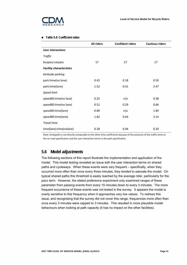
Level of Service Model for Bicycle Riders
0027 TMR LEVEL OF SERVICE MODEL (FINAL-2).DOCX Page 41
Table 5.4: Coefficient ratios
All riders Confident riders Cautious riders
User interactions
Traffic
buspass:carpass 17 27 17
Facility characteristics
Kerbside parking
park:time(no lane) 0.42 0.18 0.50
park:time(lane) 1.52 0.41 2.47
Speed limit
speed60:time(no lane) 0.25 n/a 0.38
speed80:time(no lane) 0.51 0.29 0.66
speed60:time(lane) 0.89 n/a 1.84
speed80:time(lane) 1.82 0.64 3.14
Travel time
time(lane):time(nolane) 0.28 0.44 0.20
Note: time(path) is not directly comparable to the other time coefficients because of the presence of the traffic terms in
the on‐road specification and the user interaction terms in the path specification.
5.6 Model adjustments The following sections of this report illustrate the implementation and application of the
model. This model testing revealed an issue with the user interaction terms on shared
paths and cycleways. When these events were very frequent – specifically, when they
occurred more often than once every three minutes, they tended to saturate the model. On
typical shared paths this threshold is easily reached by the average rider, particularly for the
pass term. However, the stated preference experiment only examined ranges of these
parameter from passing events from every 15 minutes down to every 3 minutes. The more
frequent occurrence of these events was not tested in the survey. It appears the model is
overly sensitive to this frequency when it approaches very low values. To redress this
issue, and recognising that the survey did not cover this range, frequencies more often than
once every 3 minutes were capped to 3 minutes. This resulted in more plausible model
behaviours when looking at path capacity (it has no impact on the other facilities).

Level of Service Model for Bicycle Riders
0027 TMR LEVEL OF SERVICE MODEL (FINAL-2).DOCX Page 42
5.7 LOS mapping The stated preference model does not output a level of service (LOS). Rather, it provides a
generalised cost (or “utility”). This cost is negative, as travelling is seen as a means to an
end9. The link that has the least negative generalised cost will be preferred by riders.
In order to map this generalised cost to LOS the tolerance to delay was used to link the
stated preference model to the contingent valuation questions on delay in the survey
(Figure 4.18). This required a number of assumptions:
the likert scales in the stated intention question map directly to levels of service,
namely that:
o a score of 1 (“Doesn’t bother me at all”) equates to LOS A, and
o a score of 5 (“Bothers me a lot”) equates to LOS F,
the median delay headway is the most appropriate measure of central tendency for
this data, and
the scores represent the thresholds at which LOS changes (e.g. the median delay
headway corresponding to a score of 5 corresponds to the threshold between LOS
E and F).
This approach gives five delay headway thresholds, each representing the threshold
between the six levels of service (A to F). The absolute generalised cost was scaled
relative to the median travel time in the survey (20 minutes), and then rebased to the
threshold between LOS D and C. This provided changes in normalised utility relative to the
thresholds between C and D. These normalised and rebased utilities, for each of the three
models are provided in Table 5.5.
Table 5.5: Utility thresholds normalised and rebased by rider type
LOS
Median
headway
(mins)
All riders Confident riders Cautious riders
Util. Util. Util. Util. Util. Util.
B 18.96 ‐1.491 0.25 ‐1.705 0.28 ‐1.272 0.23
C 9.47 ‐1.576 0.17 ‐1.799 0.19 ‐1.348 0.15
D 4.73 ‐1.745 0.00 ‐1.988 0.00 ‐1.501 0.00
E 2.36 ‐2.085 ‐0.34 ‐2.366 ‐0.38 ‐1.808 ‐0.31
F 1.18 ‐2.763 ‐1.02 ‐3.121 ‐1.13 ‐2.420 ‐0.92
Note: each row represents the lower threshold between LOS bands; for example “B” means the threshold where LOS deteriorates from A to B.
This approach allows the generalised cost output from the model to be mapped onto a LOS.
However, it is pertinent to note this relationship is nonlinear (Figure 5.2). The effect of this
9 This is one of the most significant challenges in trying to forecast recreation travel (by bicycle or any other mode). In these cases the travel itself is the purpose – travel time is, presumably, positively valued for these types of trips.

Level of Service Model for Bicycle Riders
0027 TMR LEVEL OF SERVICE MODEL (FINAL-2).DOCX Page 43
transformation is to linearise the utility-LOS relationship. This simplifies the interpretation of
the model outputs.
Figure 5.2: Relative utility and median delay headway by rider type
5.8 Developing the composite route LOS measurement The model provides a generalised cost (utility) for an individual link. These links need to be
homogenous – that is, they cannot change in any characteristic along their length (e.g.
traffic volume, width). In practice, almost all bicycle trips would involve the use of differing
types of road and path. In turn, these riders are likely to perceive the overall level of service
of their trip as a sum of the individual link levels of service. In order to develop this
composite route measure of LOS the following procedure was used:
the generalised cost for each link was calculated,
the generalised cost for each link was weighted by the travel time, and
the generalised cost was rescaled to the average travel time (20 minutes) in order
to convert to LOS.
This process was simple, but assumes the links are perceived in a purely additive manner.
It is not clear this is the case, and the stated preference surveys provide no means of
verifying (or refuting) this assumption.
E>F
D>E C>D
B>C
A>B
0
2
4
6
8
10
12
14
16
18
20
‐1.4 ‐1.2 ‐1.0 ‐0.8 ‐0.6 ‐0.4 ‐0.2 0.0 0.2 0.4
Med
ian delay headway (minutes)
Relative Utility
All riders Confident riders Cautious riders

Level of Service Model for Bicycle Riders
0027 TMR LEVEL OF SERVICE MODEL (FINAL-2).DOCX Page 44
6 Model implementation The stated choice model has been implemented as an Excel spreadsheet. This
implementation provides a user-friendly means of calculating the LOS for links and routes
without requiring an understanding of the mechanics of the underlying model. The model
consists of three worksheets:
Path interactions: allows an analyst to determine the frequency of delay (and
other user interactions) on shared paths and cycleways of specified widths and
demand (based on the previous SKM study).
Links: calculates the LOS for a link, and allows the analyst to save the link to a
database for further analysis, or incorporation into a route.
Routes: calculate the LOS for a route, consisting of a selection of links obtained
from the link database.
Screenshots from each sheet in the spreadsheet are provided in Figure 6.1.
To illustrate the use of the model, consider the following examples:
1. We are interested in the LOS of a shared path, and how it would change if it were
widened and/or segregated between modes.
a. Start with the Path interactions worksheet and enter the path width, cyclist
and pedestrian demand during the design hour, and the directional split.
b. If necessary, alter the speeds and standard distributions of the speeds.
c. Other model parameters, such as clearance distances and proportions in
groups can also be adjusted. However, these can be retained as their
default values for most situations.
d. This worksheet outputs the headways of delay, cyclist overtaking events,
pedestrian overtaking and meeting events. These values can then be
transferred to the Links worksheet in the ‘User interactions’ area. In
addition, the analyst should select the travel time on the link, the type of link
(shared path, road without facilities, road with bicycle lanes or road with
protected bicycle lane) and other features of the link.
e. Select the rider model to apply (all, confident or cautious).
f. The worksheet will then output the LOS for the link.
g. The link can be saved for later use by selecting the ‘Add to list’ button to the
left of the worksheet.
h. Scenarios can then be run, and saved as necessary, for different design
alternatives (and levels of demand).
2. We are interested in determining the route LOS.
a. Build each link using the Links worksheet, saving each to the link database
using the ‘Add to list’ button.

Level of Service Model for Bicycle Riders
0027 TMR LEVEL OF SERVICE MODEL (FINAL-2).DOCX Page 45
b. Select the Routes worksheet and build the route by selecting the links from
the left of the worksheet then clicking on ‘Add to Route’.
c. The route LOS will be displayed next to the route name.
d. If necessary, the route can be saved to the route database to the right of
the worksheet.
The spreadsheet makes it quick and easy for the non-technical user to determine the LOS
of an existing link or route, and test the likely impact of possible improvements.
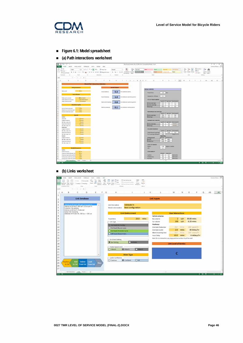
Level of Service Model for Bicycle Riders
0027 TMR LEVEL OF SERVICE MODEL (FINAL-2).DOCX Page 46
Figure 6.1: Model spreadsheet
(a) Path interactions worksheet
(b) Links worksheet

Level of Service Model for Bicycle Riders
0027 TMR LEVEL OF SERVICE MODEL (FINAL-2).DOCX Page 47
(c) Routes worksheet

Level of Service Model for Bicycle Riders
0027 TMR LEVEL OF SERVICE MODEL (FINAL-2).DOCX Page 48
7 Sensitivity testing 7.1 Outline The purpose of this section is to demonstrate the plausibility of the model through sensitivity
testing. A number of scenarios are presented to illustrate the behaviour of the model. As
the model has 14 degrees of freedom it is impossible to describe every possible scenario;
instead, the sensitivities described in this section are relative to a “typical” base condition
listed in Table 7.1. Unless otherwise stated in the discussion that follows the conditions are
as stated in this table.
Table 7.1: Base parameters in sensitivity tests
Parameter Value
Link type On road (no bicycle lane)
On street parking No kerbside parking
Speed limit 50 km/h
Bus overtaking Every 20 minutes / 3 vph
Cars overtaking Every 12 seconds / 300 vph
Incur delay Every 5 minutes / 12 per hour
7.2 Motor vehicle interactions We would expect busier roads to be less attractive to riders, and particularly to cautious
riders. Our assumption is that it is motorists travelling in the same direction as the rider,
and in the kerbside lane on multilane roads, which is the relevant volume metric in this
discussion.
For the base condition (i.e. a road with no dedicated cycling infrastructure) on quiet local
streets (around 100 cars per hour) the level of service will border between C and D for the
average rider, and be C for confident riders (Figure 7.1). For cautious riders the LOS will be
perceived as E (although close to D). That confident riders would perceive local roads
without bicycle facilities as more satisfactory than cautious riders is expected. What is
perhaps not expected is that these quiet roads would be perceived as having such an
unsatisfactory LOS for cautious riders.
The LOS deteriorates most rapidly for cautious riders (as would be expected). The LOS for
confident riders deteriorates to E at about 700 cars per hour.

Level of Service Model for Bicycle Riders
0027 TMR LEVEL OF SERVICE MODEL (FINAL-2).DOCX Page 49
Figure 7.1: Sensitivity to car volumes
The presence of buses have a more marked impact on LOS. The LOS drops rapidly as the
number of buses increases, as shown in Figure 7.2. The rate of deterioration in LOS is
marginally greater for cautious riders than confident riders; for the latter group the LOS will
be E for low bus volumes and reach F at around 22 buses per hour. For confident riders
the road without buses will be C (just) and deteriorate to E at 23 busies per hour (i.e. a bus
every 2.6 minutes).
F
E
D
C
B
A
0 200 400 600 800 1,000
Overtaking cars per hour
Level o
f Service
All riders Cautious Confident

Level of Service Model for Bicycle Riders
0027 TMR LEVEL OF SERVICE MODEL (FINAL-2).DOCX Page 50
Figure 7.2: Sensitivity to bus volumes (road with no facility)
Consider now a road with similar traffic volumes, but with on-road bicycle lanes. A road
with 300 cars per hour and no buses will have a LOS of A for both confident and cautious
riders if a bicycle lane is present (Figure 7.3). However, as would be expected, the LOS for
cautious riders will deteriorate rapidly as the bus volume increase; the LOS will be D at
around 25 buses per hour (i.e. a bus every 2.4 minutes) and E at about 40 buses per hour
(i.e. a bus every 1.5 minutes). The effect is somewhat less dramatic for confident riders; at
40 buses per hour the confident rider LOS is C (compared to E for cautious riders). This
analysis, in comparison to Figure 7.2, illustrates the sensitivity of the model to on-road
facilities.
F
E
D
C
B
A
0 20 40 60 80 100
Overtaking buses per hour
Level o
f Service
Cautious Confident All riders
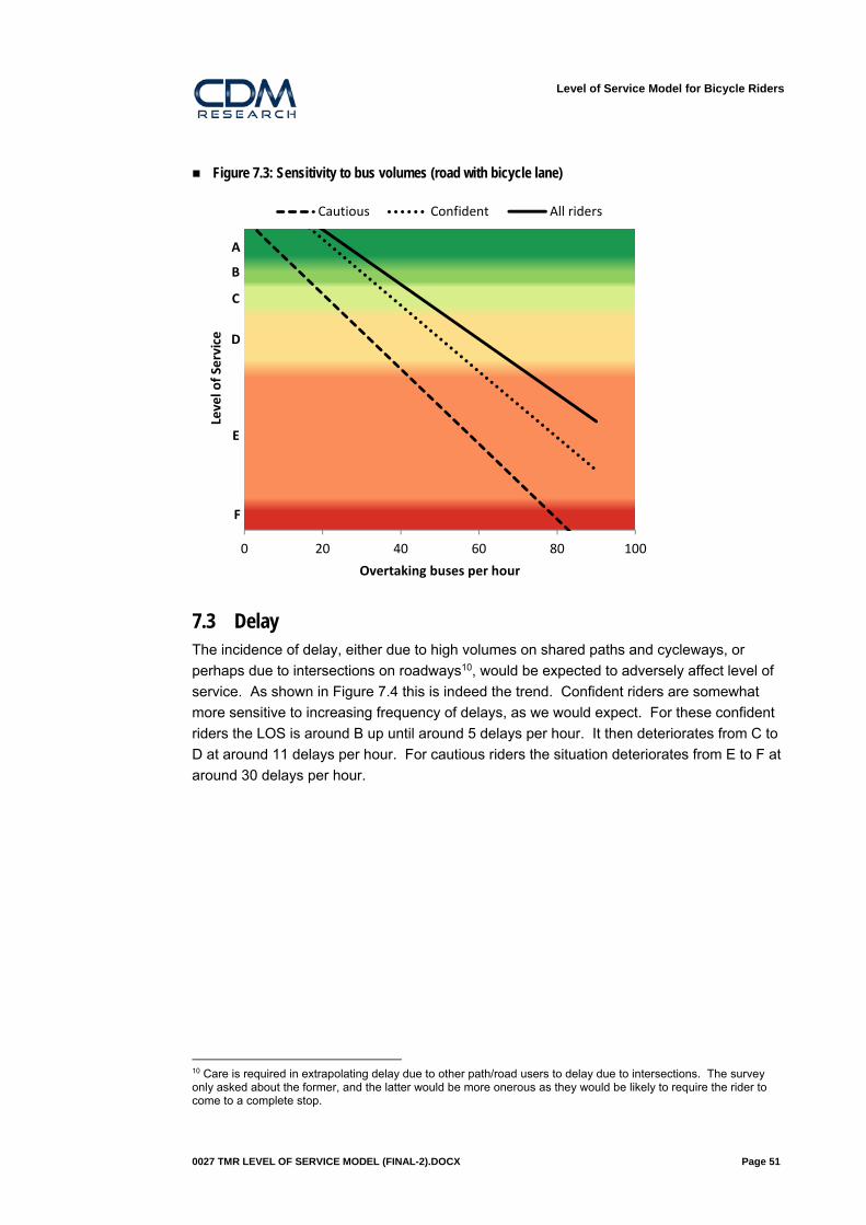
Level of Service Model for Bicycle Riders
0027 TMR LEVEL OF SERVICE MODEL (FINAL-2).DOCX Page 51
Figure 7.3: Sensitivity to bus volumes (road with bicycle lane)
7.3 Delay The incidence of delay, either due to high volumes on shared paths and cycleways, or
perhaps due to intersections on roadways10, would be expected to adversely affect level of
service. As shown in Figure 7.4 this is indeed the trend. Confident riders are somewhat
more sensitive to increasing frequency of delays, as we would expect. For these confident
riders the LOS is around B up until around 5 delays per hour. It then deteriorates from C to
D at around 11 delays per hour. For cautious riders the situation deteriorates from E to F at
around 30 delays per hour.
10 Care is required in extrapolating delay due to other path/road users to delay due to intersections. The survey only asked about the former, and the latter would be more onerous as they would be likely to require the rider to come to a complete stop.
F
E
D
C
B
A
0 20 40 60 80 100
Overtaking buses per hour
Level o
f Service
Cautious Confident All riders

Level of Service Model for Bicycle Riders
0027 TMR LEVEL OF SERVICE MODEL (FINAL-2).DOCX Page 52
Figure 7.4: Sensitivity to delay (on-road, no bicycle facility)
A similar trend is apparent on other types of bicycle facilities, although the differences
between rider groups are less significant (Figure 7.5). Both groups experience a decrease
in LOS from C to D at around 13 delays per hour (i.e. a delay every 4.6 minutes).
F
E
D
C
B
A
0 10 20 30 40 50 60
Delays per hour
Level o
f Service
Cautious Confident

Level of Service Model for Bicycle Riders
0027 TMR LEVEL OF SERVICE MODEL (FINAL-2).DOCX Page 53
Figure 7.5: Sensitivity to delay (off-road shared path)
7.4 Facility type The purpose for which the LOS is likely to be most useful is in understanding the likely
benefits of providing enroute infrastructure for bicycle riders. The sensitivity of the model to
infrastructure can be explored in a number of ways.
Firstly, consider the variation in LOS as a function of delay and facility type. This is
important in understanding, for example, at what point faster riders using a shared path may
decide to shift to an adjacent roadway if the path becomes congested (i.e. there is frequent
delay). For all riders this sensitivity is illustrated in Figure 7.6. The effect of delay
frequency for the no facility case is as per the discussion in Section 7.3. The effect of
providing bicycle facilities of increasing quality is to improve the LOS markedly for all delay
frequencies. For example, at a fairly typical delay frequency of 10 delays per hour (i.e. one
delay every 6 minutes) the LOS for the no facility case is D, but improves to A with bicycle
lanes. For shared paths the LOS would be B under this condition. A similar effect can be
observed even under conditions with very regular delays; even when a delay is
encountered every two minutes (i.e. 30 delays per hour) the LOS for the bicycle lane option
is B and for the shared path E. Protected lanes have a LOS of A for all levels of delay.
Two important conclusions can be drawn from this figure:
facility provision appears far more important than delay frequency in influencing a
riders’ LOS, and
riders appear to be more tolerant incurring delay on roads with bicycle lanes and
protected lanes than on shared paths.
F
E
D
C
B
A
0 10 20 30 40 50 60
Delays per hour
Level o
f Service
All riders Cautious Confident

Level of Service Model for Bicycle Riders
0027 TMR LEVEL OF SERVICE MODEL (FINAL-2).DOCX Page 54
The second of these conclusions is due to the lack of facility-delay interaction terms in the
model. Whether this is practically correct is less clear. One possible explanation for this
behaviour may be that riders feel they can move into the traffic lane (in the case of standard
bicycle lanes) to minimise these delays. Another possible explanation is that riders
perceive delays which occur on paths as more significant, as they will often involve
pedestrians (which may be seen as more unpredictable than passing other riders). A third
possibility is that on paths next to roads riders may be delayed at driveways, whereas on-
road motorists entering or leaving driveways are more likely to give way to the rider.
Figure 7.6: Sensitivity to delay and facility type (all riders)
The all-rider model masks significant differences between cautious and confident riders.
Figure 7.7 shows the sensitivity of delays for cautious riders on roads with bicycle lanes and
shared paths (protected lanes always have LOS A). For cautious riders delay is perceived
more negatively on roads with bicycle lanes than on shared paths. The LOS drops from C
to D when delays exceed around 10 per hour (i.e. one delay every 6 minutes) on roads with
bicycle lanes and at 12 delays per hour (i.e. one delay every 5 minutes) on shared paths.
F
E
D
C
B
A
0 10 20 30 40 50 60
Delays per hour
Level o
f Service
No facility Bicycle lane Protected lane Shared path
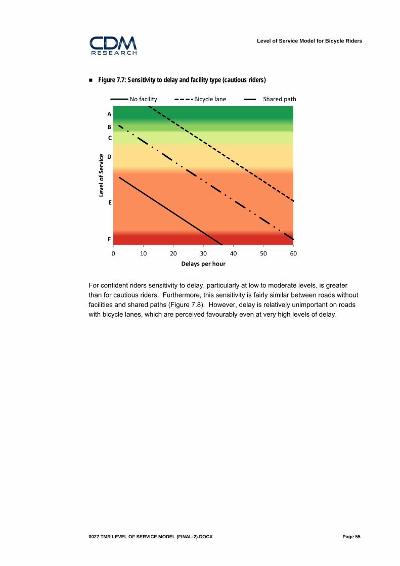
Level of Service Model for Bicycle Riders
0027 TMR LEVEL OF SERVICE MODEL (FINAL-2).DOCX Page 55
Figure 7.7: Sensitivity to delay and facility type (cautious riders)
For confident riders sensitivity to delay, particularly at low to moderate levels, is greater
than for cautious riders. Furthermore, this sensitivity is fairly similar between roads without
facilities and shared paths (Figure 7.8). However, delay is relatively unimportant on roads
with bicycle lanes, which are perceived favourably even at very high levels of delay.
F
E
D
C
B
A
0 10 20 30 40 50 60
Delays per hour
Level o
f Service
No facility Bicycle lane Shared path

Level of Service Model for Bicycle Riders
0027 TMR LEVEL OF SERVICE MODEL (FINAL-2).DOCX Page 56
Figure 7.8: Sensitivity to delay and facility type (confident riders)
7.5 Traffic volumes In this section we consider the effect of traffic volumes on infrastructure preferences.
Figure 7.9 shows that the provision of a bicycle lane improves the LOS very markedly for all
car volumes11. Protected lanes are not shown in this figure as they achieve LOS A under
all conditions12. This means that, for example, a fairly typical collector road with 600 vph
during the peak period would have a LOS D where no facility is provided, but this would
improve to A for confident riders simply through the provision of a conventional bicycle lane.
11 Note that the vehicle volumes refer only to the direction of travel and the kerbside lane. 12 This may be reasonable; a protected lane means a rider would not expect to have to interact with motorists at all at mid-block locations. Under such conditions the LOS should be reasonably independent of motorist volumes.
F
E
D
C
B
A
0 10 20 30 40 50 60
Delays per hour
Level o
f Service
No facility Bicycle lane Protected lane Shared path

Level of Service Model for Bicycle Riders
0027 TMR LEVEL OF SERVICE MODEL (FINAL-2).DOCX Page 57
Figure 7.9: Sensitivity to overtaking cars and facility type (confident riders)
The effect of car volumes and on-road facilities is similar in trend to confident riders (Figure
7.10). However, cautious riders generally allocate a lower LOS than confident riders (as
would be expected). Cautious riders are highly sensitive to car volumes (more so than
confident riders); on roads with no facility cautious riders allocate LOS E at even very low
volumes (around 20 cars per hour), although this only deteriorates to F above about 20 cars
per hour. This suggests cautious riders are reluctant to ride even on quiet residential
streets. However, when dedicated on-road space is provided in the form of bicycle lanes
cautious riders give these roads a LOS of C or above for volumes up to about 650 cars per
hour. This is somewhat surprising, but reflects the very strong preference of cautious riders
to roads with bicycle facilities. Similarly, roads with protected lanes were rated LOS A for all
traffic volumes.
F
E
D
C
B
A
0 200 400 600 800 1,000 1,200
Overtaking cars per hour
Level o
f Service
No facility Bicycle lane

Level of Service Model for Bicycle Riders
0027 TMR LEVEL OF SERVICE MODEL (FINAL-2).DOCX Page 58
Figure 7.10: Sensitivity to overtaking cars and facility type (cautious riders)
7.6 Speed limits The model shows a decrease in LOS as speed limits increase, as would be expected. At
the default urban speed limit of 50 km/h on roads with 300 cars per hour the level of service
varies from D to E (Figure 7.11). The speed60 term was insignificant in the model
estimation for the confident riders, implying these riders do not perceive a difference
between 50 and 60 km/h. However, these riders do react strongly to speed limits of 80
km/h on roads with no bicycle facilities; the LOS drops from D at 60 km/h to E at 80 km/h on
roads with the same traffic volumes.
On roads with bicycle lanes and 50 km/h speed limits both rider groups perceive LOS A. At
60 km/h this decreases to D for cautious riders, but remains A for confident riders. At 80
km/h cautious riders perceive such roads to have LOS E and confident riders LOS B. That
cautious riders would perceive such roads at 80 km/h to be highly unsatisfactory is as
expected. That confident riders would still allocate LOS B on such roads suggests a strong
tolerance amongst such riders to high speed traffic as long as they retain their own
dedicated riding space (in the form of a bicycle lane).
F
E
D
C
B
A
0 200 400 600 800 1,000 1,200
Overtaking cars per hour
Level o
f Service
No facility Bicycle lane
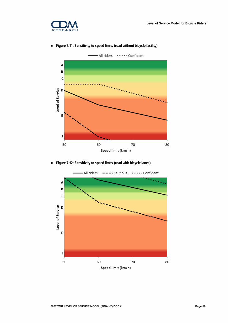
Level of Service Model for Bicycle Riders
0027 TMR LEVEL OF SERVICE MODEL (FINAL-2).DOCX Page 59
Figure 7.11: Sensitivity to speed limits (road without bicycle facility)
Figure 7.12: Sensitivity to speed limits (road with bicycle lanes)
F
E
D
C
B
A
50 60 70 80
Speed limit (km/h)
Level o
f Service
All riders Confident
F
E
D
C
B
A
50 60 70 80
Speed limit (km/h)
Level o
f Service
All riders Cautious Confident

Level of Service Model for Bicycle Riders
0027 TMR LEVEL OF SERVICE MODEL (FINAL-2).DOCX Page 60
7.7 Parking Both confident and cautious riders prefer on-road routes that do not have kerbside parking.
Typical roads with bicycle lanes without kerbside parking have an LOS of A for confident
riders and LOS B for cautious riders (Figure 7.13). If kerbside parking is present this
comfort deteriorates markedly; for cautious riders the LOS decreases to E and for confident
riders it decreases to B. The model is thus very sensitive to this parameter (at least for
cautious riders), at least for cautious riders, perhaps because of riders’ fears of car dooring
crashes.
Figure 7.13: Sensitivity to kerbside parking (roads with bicycle lanes)
7.8 Summary These sensitivity tests suggest the model is, in general, responding in a plausible way to
changes in the parameters. It suggests that cautious riders are far more sensitive to the
parameters than confident riders (as we would expect), and that all riders are highly
sensitive to the provision of dedicated cycling infrastructure on roadways. It also suggests
the all rider model is replicating the behaviour of the confident rider far more so than the
cautious rider model. This is an artefact of the model estimation process. The implication
of this, in our view, is that the policy maker should consider to whom they are designing a
facility (confident or cautious riders), to which minimum LOS they wish to achieve, and to
proceed accordingly to analyse the options. There seems little merit in apply the all rider
model for most applications.
F
E
D
C
B
A
None Kerbside
Presence of kerbside parking
Level o
f Service
All riders Cautious Confident

Level of Service Model for Bicycle Riders
0027 TMR LEVEL OF SERVICE MODEL (FINAL-2).DOCX Page 61
8 Route choices 8.1 Outline The model structure is setup in such a way that it can readily be incorporated into a
probabilistic route choice model. These models are fairly widely used in transport models.
A major advantage of logit models is that they are probabilistic; that is, they assign a
likelihood (or probability) to selecting a particular route. This is a behaviour consistent with
our expectations; for example, if there were 100 riders who had to choose between two
routes we would always expect a proportion to choose one route and the remainder the
other route. It would be very rare for all riders to choose one route, as their individual
preferences will vary. As such, in discussing route choices it is not an either-or choice but
rather a matter of determining the probability of a particular route choice.
In this section we provide simple examples of the forecast demand along completing routes
in order to further explore the model sensitivity, and how it can be applied to real-world
problems.
8.2 Example 1: Shared path vs roadway In this example we consider an example of a shared path running directly alongside a busy
road. We assume the road and path are directly adjacent such that there is no journey time
difference between the alternatives (aside from differences in delay frequency). The
question of interest is: as demand increases on the path, at what point do riders start
moving across to use the roadway instead? A secondary question is: how is this affected
by differing types of rider provision on the competing road? For simplicity we assume the
road has the characteristics listed in Figure 8.1. We consider the effects for both confident
and cautious riders.
Figure 8.1: Base road attributes
Parameter Value
Speed limit 60 km/h
Car volume 800 vph
Bus volume 6 vph
Kerbside parking None
Delay headway 5 mins
We consider here three scenarios; the road has no bicycle facility, a standard bicycle lane
and a high quality protected bicycle lane. For the situation where the road has no bicycle
lane when there are only infrequent path delays (5 per hour, or one every 12 minutes) the
path is heavily preferred by cautious riders; 86% of riders would prefer the path in this
situation (Figure 8.2). However, the preference among confident riders towards the path is
considerably lower; only 61% of confident riders would prefer the path in these conditions.

Level of Service Model for Bicycle Riders
0027 TMR LEVEL OF SERVICE MODEL (FINAL-2).DOCX Page 62
As the frequency of being delayed on the path increases, so the proportion who choose the
road (not surprisingly) increases, but only very gradually. When there are 20 delayed
passing events per hour on the path half of the confident riders would prefer the road.
However, even where there are 40 delays per hour (i.e. a delay every 1.5 minutes) around
73% of cautious riders would still prefer the path. Perhaps more surprisingly, 35% of
confident riders would also still prefer the path. We conclude that the model is insensitive to
path delays where the competing road alternative does not have any cyclist provision13.
Figure 8.2: Demand forecasts between a shared path and roadway without bicycle facilities
Consider now the case where the road has a standard bicycle lane. This increases the
attractiveness of the road among both groups of riders. As shown in Figure 8.3 just over
two thirds of cautious riders prefer the path when there are five delays per hour, and this
decreases to 50% when there are 35 delays per hour. By contrast, confident riders prefer
the road with bicycle lanes, even when there are more delays on the road than the path.
When there are five delays per hour on the path 59% of confident riders will choose the
road. This increases to 70% when delays are very frequent (40 per hour) on the path.
Again, this demonstrates that the model is more sensitive to facility provision than to the
frequency of delay.
13 This result accords with what we know from observation of sites such as Coronation Drive and the Bicentennial Bikeway; the vast majority of riders choose to use the path, and do so even during peak periods when the path is busy.
0%
10%
20%
30%
40%
50%
60%
70%
80%
90%
100%
5 10 15 20 25 30 35 40 45 50 55 60
Dem
and proportion
Path delays per hour
Confident ‐ Path Confident ‐ Road
Cautious ‐ Path Cautious ‐ Road
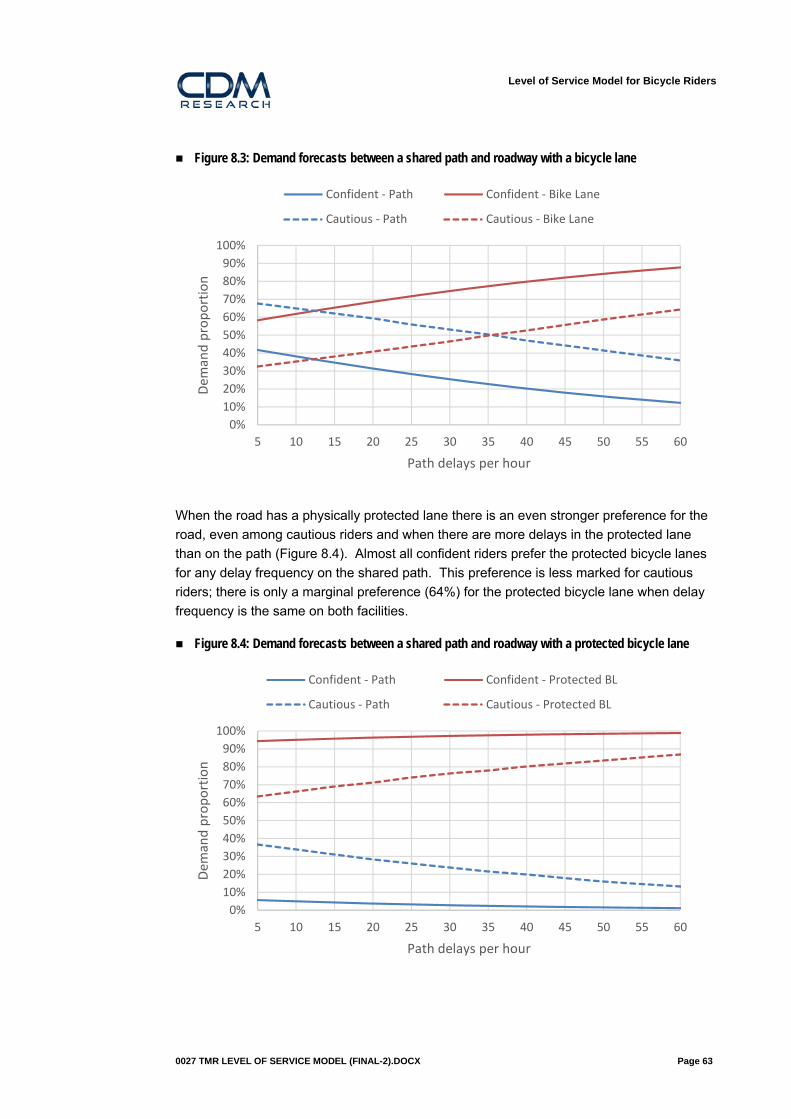
Level of Service Model for Bicycle Riders
0027 TMR LEVEL OF SERVICE MODEL (FINAL-2).DOCX Page 63
Figure 8.3: Demand forecasts between a shared path and roadway with a bicycle lane
When the road has a physically protected lane there is an even stronger preference for the
road, even among cautious riders and when there are more delays in the protected lane
than on the path (Figure 8.4). Almost all confident riders prefer the protected bicycle lanes
for any delay frequency on the shared path. This preference is less marked for cautious
riders; there is only a marginal preference (64%) for the protected bicycle lane when delay
frequency is the same on both facilities.
Figure 8.4: Demand forecasts between a shared path and roadway with a protected bicycle lane
0%
10%
20%
30%
40%
50%
60%
70%
80%
90%
100%
5 10 15 20 25 30 35 40 45 50 55 60
Dem
and proportion
Path delays per hour
Confident ‐ Path Confident ‐ Bike Lane
Cautious ‐ Path Cautious ‐ Bike Lane
0%
10%
20%
30%
40%
50%
60%
70%
80%
90%
100%
5 10 15 20 25 30 35 40 45 50 55 60
Dem
and proportion
Path delays per hour
Confident ‐ Path Confident ‐ Protected BL
Cautious ‐ Path Cautious ‐ Protected BL

Level of Service Model for Bicycle Riders
0027 TMR LEVEL OF SERVICE MODEL (FINAL-2).DOCX Page 64
This analysis suggests the riders overall are fairly insensitive to frequent path delays, at
least when the frequency delay exceeds about 10 to 15 delays per hour (i.e. one every four
to six minutes). However, the most significant finding from this sensitivity analysis is to
demonstrate the strong preference for bicycle facilities, and particularly higher quality
facilities such as protected cycleways on-road and off-road shared paths. This is
particularly true for cautious riders.
8.3 Example 2: On-road main road vs quiet street In this example we consider the scenario where there is a main road and a connected quiet
local street alternative (perhaps a bicycle boulevard). We assume the busy road has 800
vph and the quiet streets 50 vph, and that neither route has a cycling facility. Furthermore,
we assume that both routes (at least in the initial condition) have a riding time of 20
minutes. The question is: what additional travel time are riders prepared to ride in order to
use the quiet street?
As expected, when there is no travel time difference between the two routes between 60
and 75% of riders prefer the quiet street (Figure 8.5). However, this proportion drops off
rapidly for both confident and cautious riders as the riding time on the quiet street
increases. When the quiet street route takes 4 minutes longer than the busy road (i.e. 24
minutes compared with 20 minutes) then confident riders will be split evenly between the
two routes. As expected, cautious riders are prepared to divert further to use the quiet
street. When the quiet street takes 9 minutes longer then cautious riders are expected to
be evenly split between the routes.
Figure 8.5: Demand forecasts between a busy road and a quiet street
0%
10%
20%
30%
40%
50%
60%
70%
80%
90%
0 2 4 6 8 10 12 14 16 18 20
Dem
and proportion
Additional travel time (mins) on quiet street
Confident ‐ Quiet Confident ‐ Busy
Cautious ‐ Quiet Cautious ‐ Busy

Level of Service Model for Bicycle Riders
0027 TMR LEVEL OF SERVICE MODEL (FINAL-2).DOCX Page 65
8.4 Example 3: On-road vs On-road with bicycle lanes In this example we consider the scenario where there are two main roads, each with 800
vph. Both are assumed in the base case to require 20 minutes of riding time. However,
one of the roads has conventional on-road bicycle lanes. The question is: what additional
travel time are riders prepared to ride in order to use the road with bicycle lanes compared
to the road with no dedicated facility?
When there is no travel time difference between the two routes between 70 and 75% of
riders prefer the road with bicycle lanes (Figure 8.6). However, this proportion drops off
rapidly for both confident and cautious riders as the additional riding time on the route with
the bicycle lanes increases. When the road with bicycle lanes takes 10 minutes longer than
the busy road (i.e. 10 minutes compared with 20 minutes) then both groups of riders will be
split evenly between the two routes.
Figure 8.6: Demand forecasts between a busy road without facilities and a busy road with bicycle lanes
8.5 Example 3: On-road vs On-road with protected bicycle lanes This scenario is similar to the previous example, except it is now assumed one of the busy
roads has protected bicycle lanes. The question is: what additional travel time are riders
prepared to ride in order to use the road with protected bicycle lanes compared to the road
with no dedicated facility?
When there is no travel time difference between the two routes between 80 and 90% of
riders prefer the road with protected bicycle lanes (Figure 8.7). This proportion drops off
only gradually for both confident and cautious riders as the additional riding time on the
route with the bicycle lanes increases. When the road with protected bicycle lanes takes 23
minutes longer than the busy road (i.e. 43 minutes compared with 20 minutes, or more than
0%
10%
20%
30%
40%
50%
60%
70%
80%
0 5 10 15 20
Dem
and proportion
Additional travel time (mins) on route with facility
Confident ‐ No Facility Confident ‐ Bicycle Lane
Cautious ‐ No Facility Cautious ‐ Bicycle Lane

Level of Service Model for Bicycle Riders
0027 TMR LEVEL OF SERVICE MODEL (FINAL-2).DOCX Page 66
twice as long) then confident riders will be split evenly between the two routes. For
cautious riders even when the protected bicycle lane route takes an additional 30 minutes
just over 70% of cautious riders will still choose the protected bicycle lane. This result for
both confident and cautious riders would suggest that riders are prepared to divert very
significant distances in order to use higher quality on-road facilities (compared to roads
without any facility).
Figure 8.7: Demand forecasts between a busy road without facilities and a busy road with a protected bicycle lane
0%
10%
20%
30%
40%
50%
60%
70%
80%
90%
100%
0 5 10 15 20 25 30
Dem
and proportion
Additional travel time (mins) on route with facility
Confident ‐ No Facility Confident ‐ Protected Lane
Cautious ‐ No Facility Cautious ‐ Protected Lane

Level of Service Model for Bicycle Riders
0027 TMR LEVEL OF SERVICE MODEL (FINAL-2).DOCX Page 67
9 Practical examples 9.1 Outline The purpose of this section is to illustrate the application of the model by example. The
links and routes chosen are hypothetical, and serve only to illustrate the application of the
model – they are not intended to be realistic examples.
9.2 Link examples Links are individual sections of road or path; for example, a roadway section between two
signalised intersections. It is assumed these links have common characteristics along their
length.
9.2.1 Shared use path
Scenario
A shared path in an inner city area is being resurfaced. It is currently 2.5 m wide and
carries 400 cyclists in the peak hour (300 in the peak direction, 100 in the contrapeak) and
50 pedestrians (25 in each direction). It is forecast that in five years the path will carry 700
cyclists in the peak hour (525 in the peak direction, 175 in the contrapeak) and 150
pedestrians (75 in each direction).
Objective
What width should the path be rebuilt to in order to achieve a minimum LOS C for the
confident rider, and is it most efficient to rebuild the path as a shared path or segregated
between modes?
Results
The path interaction calculator, using default inputs, returns a delay headway of 1.9 minutes
for a typical rider under current conditions (that is, a rider riding in the peak direction). This,
along with the other interaction headways, entered into the link LOS calculator gives a
current LOS E. This poor LOS is attributable to the frequent delays the typical rider would
experience (i.e. 32 delays per hour).
If the path were rebuilt to its current width of 2.5 m the LOS would deteriorate to F in five
years, mainly as a result of the average delay headway decreasing from 1.9 minutes now to
every 20 seconds in the future. If instead the path were widened to a 3.0 m shared path the
average rider would be delayed once every 1.2 minutes, which would be insufficient to
improve LOS beyond F. This would be only marginally better for riders than the do-nothing
scenario. Moreover, it would still not achieve the desired LOS C threshold. Widening
further to 4.0 m would significantly reduce the delay (now every 16 minutes) and would
provide LOS C. However, it would not eliminate the interaction with other riders and
pedestrians. The latter contributes much to LOS. As an alternative to widening the path
still further (which seems unreasonable given the level of demand), an alternative would be
to provide a segregated (or separated cycleway and footpath. If this approach were taken,
and a cycleway of 2.5 m provided, the average rider would experience delays every 2.8

Level of Service Model for Bicycle Riders
0027 TMR LEVEL OF SERVICE MODEL (FINAL-2).DOCX Page 68
minutes. However, the absence of interactions with pedestrians would maintain the LOS at
C. In other words, rider would be trading off increased delay frequency against not having
to interact with pedestrians. If the cycleway instead was 3.0 m there would be delays every
15 minutes and the LOS would increase to A. The dominant disutility in this configuration is
the meeting events with oncoming bicycle riders. The model is insensitive to the lateral
clearances between riders; we would expect as the path is widened oncoming riders would
give one another more space – which would not be perceived as onerous by either rider.
However, the model currently ignores this effect and instead treats all meeting events –
whether on a 2.5 m path or 4.0 m path (or wider) as identical. This is a limitation of the
model, and would need to be handled qualitatively by the analyst.
9.2.2 Collector road
Scenario
Consider a typical collector road, with 400 cars per hour during the peak and 6 buses per
hour. The road currently does not have any bicycle facility, but has kerbside parking and
has a 60 km/h speed limit. Riders will incur a delay on average once every 6 minutes.
Objective
Achieve a minimum LOS C for cautious riders by installing some of bicycle facility and/or
adjusting the road configuration (i.e. speed limit, kerbside parking).
Results
The road in the base configuration has a LOS F for cautious riders (and D for confident
riders). The following three options would all meet the objective of providing LOS C as a
minimum to cautious riders:
installing a standard on-road bicycle lane, removing kerbside parking and reducing
the speed limit to 50 km/h would result in LOS A,
installing a physically protected bicycle lane would result in LOS A, and
installing a standard on-road bicycle lane and changing traffic conditions such that
the peak hour car volume is reduced to 110 vehicles per hour would achieve LOS
C.
9.2.3 Arterial road
Scenario
Consider a typical arterial road, with 800 cars per hour during the peak (in the main flow
direction, in the kerbside lane) and 20 buses per hour. The road does not currently have
any bicycle facility, nor does it have kerbside parking. The speed limit is 80 km/h. Riders
will incur a delay on average once every 10 minutes.
Objective
Achieve a minimum LOS C for confident riders.
Results

Level of Service Model for Bicycle Riders
0027 TMR LEVEL OF SERVICE MODEL (FINAL-2).DOCX Page 69
The road in the base configuration has a LOS E for confident riders (and F for cautious
riders). The following treatments would meet the objective of minimum LOS C for confident
riders:
a physically protected bicycle lane would achieve LOS A (note that a standard
bicycle lane would only achieve LOS D), or
a standard on-road bicycle lane and a 60 km/h speed limit.
9.2.4 Kerbside parking
Scenario
A collector road (60 km/h, 300 vph, 3 buses per hour) has a wide kerbside lane where
parking is permitted. There is a history of car dooring related crashes along this stretch of
road, which we assume takes 20 minutes to ride along. There are opportunities to provide
an alternative shared path or protected bicycle lane on a parallel route. Which alternative
would encourage most riders to choose the alternative?
Objective
Achieve at least LOS C on the alternative route, and shift at least 50% of confident riders to
the other route.
Results
The LOS in the current condition with kerbside parking is D for confident riders. If kerbside
parking were removed the LOS would increase to C, meeting the objective. However, if the
parking were to be retained the alternatives would, presumably, result in some additional
travel time for the rider. Both the shared path and protected bicycle lane alternatives would
have LOS A. However, this is only an assessment of the sense of comfort on these routes;
it does not judge the relative attractiveness of these alternatives compared to the collector
road. If we assume the shared path takes 30 minutes, then we would expect around 48%
of riders to divert to this alternative. If instead a protected lane on a parallel road was
introduced, and this had a 25 minute travel time, then 74% of riders would divert to that
alternative. Naturally, if the difference in travel times were less the proportion diverting
would be greater (and vice versa).
9.3 Route examples Routes are collections of links; each link may differ along the link. This is more akin to a
real world scenario where, for example, a rider may travel along a local road, onto a
collector road then onto a shared path. The purpose of this section is to illustrate the
application of the model to determine a LOS for a complete route. What is excluded from
consideration, but would be important in practice, is the influence of intersections on the
route LOS.
9.3.1 Road corridor
Scenario
Consider a typical commuter rider (who we consider to be confident) riding to work:

Level of Service Model for Bicycle Riders
0027 TMR LEVEL OF SERVICE MODEL (FINAL-2).DOCX Page 70
They ride 5 minutes km along a residential road from their home (say 100 vph, 50
km/h speed limit),
They then join a collector road with 500 vph, 4 buses per hour, kerbside parking
and a 60 km/h speed limit. The journey on this collector takes 10 minutes.
From the collector road the rider joins an arterial road, where there is a standard
bicycle lane, 80 km/h speed limit and no kerbside parking. There are 800 vph and
10 buses per hour. This leg takes 10 minutes.
They then leave the arterial and turn onto a quiet local road (100 vph, 50 km/h
speed limit) for the final 5 minutes to their workplace. Kerbside parking is prohibited
on this street.
Objective
Determine the LOS for this route, and each link, and then identify options which would
improve the route LOS to a minimum of C.
Results
Firstly, we can calculate the link LOS:
The local street from home has LOS C. This is strongly influenced by the presence
of kerbside parking; without parking the LOS would be A.
The collector road has LOS D. Again, this poor LOS is motivated in part by the
presence of kerbside parking; without the parking the LOS would improve to C.
The arterial road LOS is C; the presence of the bicycle lane (and absence of
kerbside parking) are positives but these are compensated by the high traffic
volume and, particularly, traffic speed limit (80 km/h). For reference, the same road
would have LOS A if the speed limit were 60 km/h. Conversely, without the bicycle
lane it would be LOS E with a 80 km/h speed limit and D with a 60 km/h speed limit.
The local road at the workplace end of the trip is the same as at the home end of
the trip, except that kerbside parking is not present. This provides a LOS of A.
The overall LOS for the trip is calculated as D; this is the time weighted average LOS for the
route. The following treatments would achieve a route LOS of C:
If we were to reduce the arterial road speed limit from 80 km/h to 60 km/h this
would improve the LOS to A on that link. This intervention of itself would be
sufficient to provide a route LOS of C.
If we were able to install conventional bicycle lanes on the collector road this would
increase the LOS on that link from D to A. This would be sufficient to increase the
route LOS to C.
If were able to upgrade the bicycle lanes on the arterial road to protected lanes this
would increase the LOS on the arterial road to A, and increase the route LOS to C.
If it were possible to install a shared path alongside the collector road, and we
assume travel times along this shared path are the same as along the road, then
the LOS of the path (assuming delays every 10 minutes) would be A, and the route
LOS would be C.

Level of Service Model for Bicycle Riders
0027 TMR LEVEL OF SERVICE MODEL (FINAL-2).DOCX Page 71
This example illustrates the usefulness of the model in identifying potential treatments
which would achieve a desired route LOS. Clearly, what it does not do is identify the
practicality or cost effectiveness of any particular measure. Nonetheless, it provides the
analyst with the opportunity to test different scenarios and to use the outputs to build the
case around a particular intervention.
9.3.2 Combined on- and off-road route
Scenario
The previous example involved equal proportions of the travel time on three different types
of link (quiet street, collector and arterial roads). This example demonstrates the effect of
links of very different lengths.
Imagine a resident of, say, Toowong who rides into the Brisbane CBD. They are a cautious
rider. Their current route is as follows:
5 minutes on Sylvan Road to the Bicentennial Bikeway – say 300 vph and no
buses; there are on-road bicycle lanes and no kerbside parking. The speed limit is
60 km/h.
20 minutes on the Bicentennial Bikeway to the CBD. Assume the bikeway is 3.0 m
wide14, there are 800 riders in the peak hour (75% heading towards the CBD) and
100 pedestrians (50% heading towards the CBD).
4 minutes on Adelaide Street to their workplace, where they have no dedicated
cyclist provision and must interact with many buses (100 vph) but relatively few cars
(100 vph).
Objective
Determine the current LOS for this route, and each link, and then identify options which
would improve the LOS to a minimum of C.
Results
The current link LOS are:
The LOS on Sylvan Road is A, thanks in large part to the presence of the bicycle
lane.
The demand on the Bicentennial Bikeway will present delays to the rider every 2.4
minutes. They will pass a pedestrian every 20 seconds. This will result in LOS E.
On Adelaide Street the high volume of buses and the absence of bicycle facilities
will result in LOS F.
The overall route LOS will be E, motivated in large part by the short (but very unfavourable)
riding along Adelaide Street.
Consider firstly improvements to the Bicentennial Bikeway. Assume, as has been done, the
cycleway is widened and segregated between modes. If we assume riders and pedestrians
14 Much of the Bicentennial Bikeway has been widened and segregated between modes. The purpose of this hypothetical example is to illustrate the impact that treatment has had on route LOS.

Level of Service Model for Bicycle Riders
0027 TMR LEVEL OF SERVICE MODEL (FINAL-2).DOCX Page 72
no longer need to interact on the path then the average time between delay will increase to
every 15.5 minutes. The impact will be to improve the LOS to C. Further improvements in
LOS would require less interaction between riders. In part, this result seems unduly
conservative. However, it may reflect (in part) reticence from cautious riders to have to
closely interact with faster riders on cycleways.
The upgrades to the Bicentennial Bikeway would however not improve the route LOS from
E. The main issue remains the short but unattractive section of riding along Adelaide
Street.
Installing conventional bicycle lanes along Adelaide Street would, presumably, improve
conditions marginally for riders. However, cautious riders would continue to perceive riding
conditions as poor – LOS would remain F under this condition. However, installing
protected bicycle lanes and reducing the speed limit from 60 km/h to 50 km/h would
improve the LOS to D. Furthermore, this (in combination with the widened and segregated
Bicentennial Bikeway) would improve the route LOS to C.

Level of Service Model for Bicycle Riders
0027 TMR LEVEL OF SERVICE MODEL (FINAL-2).DOCX Page 73
10 Further work The purpose of this section is to briefly describe possible avenues for further work.
10.1 Intersection LOS Intersections clearly play a role in how riders perceive on-road routes. This is particularly
true for roundabouts and intersections with turning lanes or slip lanes. Intersections were
not part of this study, and so have been ignored in the estimation of link and route LOS.
Clearly, the analyst will need to consider the intersections in any practical use of this model
– most probably through some qualitative method.
The wide range of intersection designs, and the likely importance of detail design elements
within each intersection design in influencing LOS, would complicate the stated preference
method used in the present study. However, just as for this mid-block study, it may be
possible to use a stated preference method (or some other, simpler, ranking method) to rate
generic intersection designs. This could then readily be incorporated into the existing
spreadsheet-based model, allowing analysts to build routes of links and intersections.
10.2 Revealed preference calibration The sensitivity of the model developed in this study appear, in general, to be reasonable.
Nonetheless, there may be concern about the high sensitivity to bicycle facilities and,
possibly, other attributes such as kerbside parking. That a stated preference model would
have high sensitivities is not unexpected, given the hypothetical nature of the scenarios
presented to respondents.
A theoretically superior method is to use revealed preference data on route choices. These
revealed preferences are what riders actually do rather than what they say they would do
(i.e. stated preferences). There are several recent examples of doing this with rider route
choice data, such as Portland (USA) and in Switzerland. However, there are three very
significant technical difficulties in estimating route choice models from revealed preference
data:
there is limited data on rider route choices,
there is insufficiently detailed data on link attributes (e.g. traffic volume, presence of
kerbside parking) to readily estimate route choice models, and
there are technical issues associated with the selection of the route choice set and
overlapping paths.
We now briefly discuss each of these issues.
Rider route choices
The only information we have on rider route choices comes from surveys or GPS-based
methods such as smartphone apps (e.g. RiderLog) or logging and training software such as
Strava. Surveys tend to provide weak route information, as they require a rider to trace
their route on a map. This route may be simplified compared to their actual route, and there

Level of Service Model for Bicycle Riders
0027 TMR LEVEL OF SERVICE MODEL (FINAL-2).DOCX Page 74
is the difficulty of converting a line drawn on a paper map to digital form. The latter problem
can be rectified by using tablet computers and online maps.
GPS-based methods are probably superior to survey methods, as they are not subject to
individual recall or simplification. However, the devices themselves have technical
limitations (e.g. canyon effects in city centres) and there is the challenge of cleaning the
GPS waypoints and snapping them to a road network. Most critically though is the
challenge of ensuring the sample is unbiased. Both RiderLog and software such as Strava
are reliant to self-selection; the rider chooses to download and use the app of their own
accord. This will invariably result in a bias, probably towards confident riders who are
serious about their riding15.
These caveats aside, there is undoubtedly strong potential for the use of GPS-based route
logging from smartphones. Furthermore, such data is complimentary to permanent counts
(which provide counts, but not routes) and may be used in conjunction with Wi-Fi /
Bluetooth detection systems to validate and expand these biased samples.
Link attribute data
Once a set of route data has been collected the next issue is to identify the characteristics
of the chosen route, and of the unchosen routes (see below). The advantage of
hypothetical methods is that we can explicit state the link conditions. In revealed
preference data we are unlikely to have these characteristics. For example, we may only
know traffic volumes on main roads (not local roads) and perhaps only daily counts (rather
than the volume at the time when the rider actually used the road). We may also not have
complete, or current, knowledge of the presence of bicycle facilities or kerbside parking.
The other technical issue is the correlation between attributes that invariably occur in
revealed preference data. For example, there will be correlation between speed limits and
traffic volumes – high volume roads are also likely to be higher speed, as they will
disproportionately be arterial roads. These correlations introduce problems in estimating
route choice models.
Route choice sets and overlapping paths
Route choice models require information on the chosen route and on unchosen routes. The
problem that commonly arises is that for a typical urban area there will be many thousands
of route choices between any two points16. Most of these will be highly improbable (e.g.
Kangaroo Point to Fortitude Valley via Mount Gravatt) or be minor variations on other
routes. There are methods to identify appropriate route choice sets for estimation, but
these methods remain subject of considerable academic research.
15 This is particularly true for Strava, which has a strong following among training riders. There are probably very few riders who use their bicycle to ride to the shops, or with their children, who use Strava. The same is probably also true of RiderLog, but to a somewhat lesser extent given the breadth of the Bicycle Network membership for which this app was designed. 16 Indeed, in theory, one could identify millions of different routes between any two points on a complex road network.

Level of Service Model for Bicycle Riders
0027 TMR LEVEL OF SERVICE MODEL (FINAL-2).DOCX Page 75
The other issue concerns the many route choices which will vary only marginally from one
another. For example, two 10 km routes that are identical except for a 100 m section where
a rider may divert down a side street (perhaps to avoid an intersection). These routes are
not independent. Handling these routes with overlapping paths in model estimation is,
again, a subject of ongoing research.

Level of Service Model for Bicycle Riders
0027 TMR LEVEL OF SERVICE MODEL (FINAL-2).DOCX Page 76
11 References Alta Planning + Design (2008) Cycle Zone Analysis (CZA): A New Bicycle Transportation
Planning Tool.
http://www.altaplanning.com/App_Content/files/pres_stud_docs/Cycle%20Zone%20Present
ation%20-%20PWPB%202008.pdf (accessed 26/8/2013).
Aurecon (2010) Cycling Evaluation Review System: Hoddle Street Planning Study.
http://consult.vicroads.vic.gov.au/document/show/10 (accessed 26/8/2013).
Bicycle Network (2012) Level of Service Audit Tool for bikes.
http://www.bicyclenetwork.com.au/media/vanilla/file/LOS_AITPM_Presntn_Feb13.pdf
(accessed 26/8/2013).
Epperson, B. (1994) “Evaluating the Suitability of Roadways for Bicycle Use: Towards a
Cycling Level of Service Standard”. Transportation Research Record 1438, TRB, National
Research Council, Washington D.C.
Jensen, S. U. (2007) “Pedestrian and Bicyclist Level of Service on Roadway Segments”.
Transportation Research Record 2031, TRB, National Research Council, Washington D.C.
Jensen, S. U. (2013) “Pedestrian and Bicycle Level of Service at Intersections,
Roundabouts and other Crossings”. TRB Annual Meeting, Washington D.C.
SFDPH (2009) Bicycle Environmental Quality Index (BEQI) – Draft Report. San Francisco
Department of Public Health. http://www.sfphes.org/component/jdownloads/finish/19-
beqi/91-bicycle-environmental-quality-index-report/0?Itemid=0 (accessed 26/8/2013).
SKM (2010) Bicycle and Pedestrian Capacity Model: North Brisbane Cycleway
Investigation. Draft Report for Queensland Department of Transport and Main Roads.
http://www.cbdbug.org.au/wp-content/uploads/north-brisbane-cycleway/135-00825-file7.pdf
(accessed 4/11/2013).
Urban Systems (2012) Cycling Analysis in Metro Vancouver (Cycle Zone Analysis).
http://www.vancouvergis.org/docs/Urban_Systems_Cycle_Zone_Analysis.pdf (accessed
26/8/2013).