@let@token Belief Propagation & Beyond

IntroductionPlanar Graphical ModelsThe Story of Permanent

Belief Propagation & Beyond

Michael (Misha) Chertkov

Center for Nonlinear Studies & Theory Division, LANL& New Mexico Consortium

Workshop on Frontiers of Controls, Games, and NetworkScience with Civilian and Military Applications

UT Austin, February 19, 2010

http://cnls.lanl.gov/~chertkov/Talks/IT/bp&beyond.pdf Belief Propagation & Beyond

http://cnls.lanl.gov/~chertkov/Talks/IT/bp&beyond.pdf


Outline

1 IntroductionGraphical ModelsMessage Passing/ Belief PropagationGauge Transformations & Loop Calculus

2 Planar Graphical ModelsDimer and Ising Models on Planar GraphsPlanar (and surface) graphical models which are det-easy

3 The Story of PermanentBP for PermanentLoop Calculus, Lower and Upper Bounds for Permanent




Graphical ModelsMessage Passing/ Belief PropagationGauge Transformations & Loop Calculus

Binary Graphical Models

Forney style - variables on the edges

P(~σ) = Z−1∏a

fa(~σa)

Z =∑σ

∏a

fa(~σa)︸︷︷︸partition function

fa ≥ 0

σab = σba = ±1

~σ1 = (σ12, σ14, σ18)

~σ2 = (σ12, σ23)

Most Probable Configuration = Maximum Likelihood =Ground State: arg maxP(~σ)

Marginal Probability: e.g. P(σab) ≡∑

~σ\σabP(~σ)

Partition Function: Z – Our main object of interest

Examples





BP is Exact on a Tree Bethe ’35, Peierls ’36

1 2

5

6

4 3

Z 51(σ51) = f1(σ51), Z 52(σ52) = f2(σ52),

Z 63(σ63) = f3(σ63), Z 64(σ64) = f4(σ64)

Z 65(σ56) =∑~σ5\σ56

f5(~σ5)Z51(σ51)Z52(σ52)

Z =∑~σ6

f6(~σ6)Z63(σ63)Z64(σ64)Z65(σ65)

Zba(σab) =∑~σa\σab

fa(~σa)Zac(σac)Zad(σad) ⇒ Zab(σab) = Aab exp(ηabσab)

Belief Propagation Equations∑~σa

fa(~σa) exp(∑c∈a

ηacσac) (σab − tanh (ηab + ηba)) = 0

e.g. Thouless-Anderson-Palmer (1977) Eqs.





Belief Propagation (BP) and Message Passing

Apply what is exact on a tree (the equation) to other problems on graphs withloops [heuristics ... but a good one]

To solve the system of N equations is EASIER then to count (or to choose oneof) 2N states.

Bethe Free Energy formulation of BP [Yedidia, Freeman, Weiss ’01]

Minimize the Kubblack-Leibler functional

F{b({σ})} ≡∑{σ}

b({σ}) lnb({σ})L({σ})

Difficult/Exact

under the following “almost variational” substitution” for beliefs:

b({σ}) ≈∏

i bi (σi )∏

j bj (σj )∏(i,j) bj

i (σji )

[tracking]Easy/Approximate

Message Passing is a (graph) DistributedImplementation of BP

Graphical Models = the language





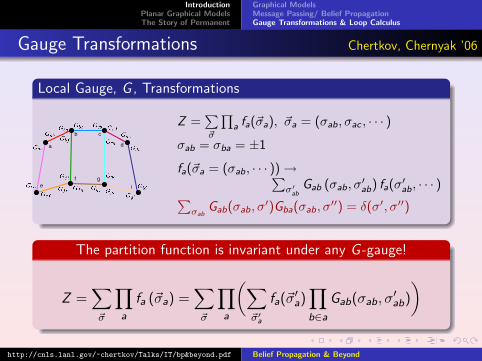
Gauge Transformations Chertkov, Chernyak ’06

Local Gauge, G , Transformations

a

b c

e

d

if g

Z =∑~σ

∏a fa(~σa), ~σa = (σab, σac , · · · )

σab = σba = ±1

fa(~σa = (σab, · · · ))→∑σ′ab

Gab (σab, σ′ab) fa(σ′ab, · · · )∑

σabGab(σab, σ

′)Gba(σab, σ′′) = δ(σ′, σ′′)

The partition function is invariant under any G -gauge!

Z =∑~σ

∏a

fa (~σa) =∑~σ

∏a

(∑~σ′a

fa(~σ′a)∏b∈a

Gab(σab, σ′ab)

)





Belief Propagation as a Gauge Fixing Chertkov, Chernyak ’06

Z =∑~σ

∏a

fa (~σa) =∑σ

∏a

(∑~σ′a

fa(~σ′a)∏b∈a

Gab(σab, σ′ab)

)

Z = Z0(G )︸︷︷︸ground state

~σ = +~1

+∑

all possible colorings of the graph

Zc(G )

︸︷︷︸~σ 6=+~1, excited states

Belief Propagation Gauge ∀a & ∀b ∈ a :

∑~σ′a

fa(~σ′)G(bp)ab (σab = −1, σ′ab)

c 6=b∏c∈a

G(bp)ac (+1, σ′ac) = 0

No loose BLUE=colored edges at any vertex of the graph!





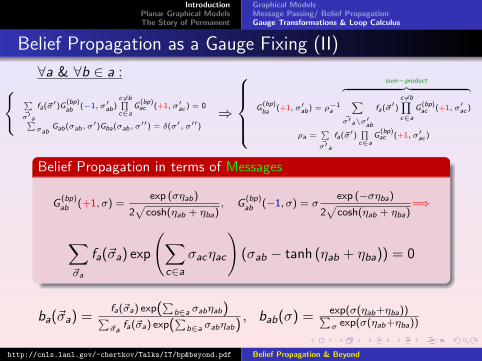
Belief Propagation as a Gauge Fixing (II)

∀a & ∀b ∈ a :{ ∑~σ′a

fa(~σ′)G (bp)ab

(−1, σ′ab)c 6=b∏c∈a

G(bp)ac (+1, σ′ac ) = 0∑

σabGab(σab, σ

′)Gba(σab, σ′′) = δ(σ′, σ′′)

⇒

G(bp)ba

(+1, σ′ab) = ρ−1a

sum−product︷︸︸︷∑~σ′a\σ′ab

fa(~σ′)c 6=b∏c∈a

G (bp)ac (+1, σ′ac )

ρa =∑~σ′a

fa(~σ′)∏

c∈aG

(bp)ac (+1, σ′ac )

Belief Propagation in terms of Messages

G(bp)ab (+1, σ) =

exp (σηab)

2√

cosh(ηab + ηba), G

(bp)ab (−1, σ) = σ

exp (−σηba)

2√

cosh(ηab + ηba)=⇒

∑~σa

fa(~σa) exp

(∑c∈a

σacηac

)(σab − tanh (ηab + ηba)) = 0

ba(~σa) =fa(~σa) exp(

∑b∈a σabηab)∑

~σafa(~σa) exp(

∑b∈a σabηab)

, bab(σ) = exp(σ(ηab+ηba))∑σ exp(σ(ηab+ηba))





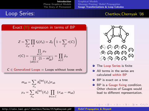
Loop Series: Chertkov,Chernyak ’06

Exact (!!) expression in terms of BP

Z =∑~σσ

∏a

fa(~σa) = Z0

(1 +

∑C

r(C)

)

r(C) =

∏a∈C

µa∏(ab)∈C

(1−m2ab)

=∏a∈C

µa

C ∈ Generalized Loops = Loops without loose ends

mab =∑~σa

b(bp)a (~σa)σab

µa =∑~σa

b(bp)a (~σa)

∏b∈a,C

(σab −mab)

The Loop Series is finite

All terms in the series arecalculated within BP

BP is exact on a tree

BP is a Gauge fixing condition.Other choices of Gauges wouldlead to different representation.





BP (Loop Calculus) + results (’06-...)

... not discussed today ...

Exact Algorithm & Efficient Truncation of Loops [V. Gomez, J.M. Mooij, H.J.Kappen ’06]

Improving LP/BP decoding with loops [MC ’07]

Loop Tower (general finite alphabet) [VC,MC ’07]

Low bound on partition function for some special (attractive) graphical models[Sudderth, Wainwright, Willsky ’07]

Fermions & Loops, e.g. monomer-dimer =series over dets [VC,MC ’08]

Counting Independent Sets Using the Bethe Approximation [V. Chandrasekaran,MC, D. Gamarnik, D. Shah, J. Shin ’09]

Beyond Gaussian BP (det=BP*det & orbit product) [J. Johnson, VC, MC’09-’10]

... also ... Particle Tracking (Learning with BP), Phase Transitions in PowerGrids, Interdiction and OTHER APPLICATIONS

BP+ and gauges on planar and surface graphs [VC, MC ’09-’10]

BP+ for Permanents (of non-negative matrices) [Y. Watanabe, MC ’09]




Dimer and Ising Models on Planar GraphsPlanar (and surface) graphical models which are det-easy

Outline








Glassy Ising & Dimer Models on a Planar Graph

Partition Function of Jij ≷ 0 Ising Model, σi = ±1

Z =∑~σ

exp

(∑(i ,j)∈Γ Jijσiσj

T

)

Partition Function of Dimer Model, πij = 0, 1

Z =∑~π

∏(i ,j)∈Γ

(zij)πij∏i∈Γ

δ

∑j∈i

πij , 1

perfect matching





Ising & Dimer Classics

L. Onsager, Crystal Statistics, Phys.Rev. 65, 117 (1944)

M. Kac, J.C. Ward, A combinatorial solution of the Two-dimensional IsingModel, Phys. Rev. 88, 1332 (1952)

C.A. Hurst and H.S. Green, New Solution of the Ising Problem for aRectangular Lattice, J.of Chem.Phys. 33, 1059 (1960)

M.E. Fisher, Statistical Mechanics on a Plane Lattice, Phys.Rev 124, 1664(1961)

P.W. Kasteleyn, The statistics of dimers on a lattice, Physics 27, 1209 (1961)

P.W. Kasteleyn, Dimer Statistics and Phase Transitions, J. Math. Phys. 4, 287(1963)

M.E. Fisher, On the dimer solution of planar Ising models, J. Math. Phys. 7,1776 (1966)

F. Barahona, On the computational complexity of Ising spin glass models,J.Phys. A 15, 3241 (1982)





Pfaffian solution of the Matching problem

1

2

3

4Z = z12z34+z14z23 =

√DetA = Pf[A]

A =

0 −z12 0 −z14

+z12 0 +z23 −z24

0 −z23 0 +z34

+z14 +z24 −z34 0

Odd-face [Kasteleyn] rule (for signs)

Direct edges of the graph such thatfor every internal face the number ofedges oriented clockwise is odd

1

2

3

4

1

2

3

4

1

2

3

4

Fermion/Grassman Representation





Planar Spin Glass and Dimer Matching Problems

The Pfaffian formula with the “odd-face” orientation rule extendsto any planar graph thus proving constructively that

Counting weighted number of dimer matchings on a planargraph is easy

Calculating partition function of the spin glass Ising model ona planar graph is easy

Planar is generally difficult [Barahona ’82]

Planar spin-glass problem with magnetic field is difficult

Dimer-monomer matching is difficult even in the planar case





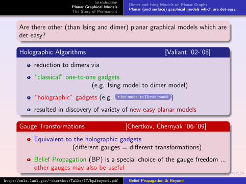
Are there other (than Ising and dimer) planar graphical models which aredet-easy?

Holographic Algorithms [Valiant ’02-’08]

reduction to dimers via

“classical” one-to-one gadgets(e.g. Ising model to dimer model)

“holographic” gadgets (e.g. Ice model to Dimer model )

resulted in discovery of variety of new easy planar models

Gauge Transformations [Chertkov, Chernyak ’06-’09]

Equivalent to the holographic gadgets(different gauges = different transformations)

Belief Propagation (BP) is a special choice of the gauge freedom ...other gauges may also be useful





BP+ for Planar [degree ≤ 3]

Loop Series (general)[MC,Chernyak ’06]

Z = Z0 · z , z ≡ 1 +∑

C rC

Summing 2-regular (closed curve) partition is det-easy!![MC,Chernyak,Teodorescu ’08]

Zs = Z0 · zs , zs = 1 +∑∀a∈C , |δ(a)|C =2

C∈G rC [JSTAT ’08]

Efficient Approximate Scheme[Gomez,MC,Kappen ’09]

http://arXiv.org/abs/0901.0786

UAI, 2009 + to appear in JML ’10

erro

r Z

10−10

10−5

100 β = 0.1

BP errorZ∅ error

ZΨ

−8

−6

−4

−2

0

2x 10

−12

erro

r Z

10−10

10−5

100 β = 0.5

ZΨ

−15

−10

−5

0

5x 10

−8

l (loop terms)

erro

r Z

100

102

104

10−10

10−5

100

p (pfaffian terms)

β = 1.5

100

102

104

ZΨ

p (pfaffian terms)10

010

110

2−5

0

5x 10

−4


http://arXiv.org/abs/0901.0786




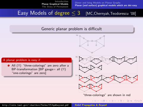
Easy Models of degree ≤ 3 [MC,Chernyak,Teodorescu ’08]

Generic planar problem is difficult

A planar problem is easy if

All (!!) “three-colorings” are zero after aBP-transformation [BP gauge= all (!!)“one-colorings” are zero]

a

b

c d e

(a)

(b)

(c)

f

g

hji

k

l

“three-colorings” are shown in red





Easy Models of degree ≤ 3 (II)

To describe the family of easy edge-binary models of degree not largerthan three (partition function is reducible to Pfaffian of a|G1| × |G1|-dimensional skew-symmetric matrix) one needs to:

Item #1: Generate an arbitrary factor-function set which

satisfies: ∀a : W (a)(~σa) = 0 if∑

b∼a σab 6= 0(mod 2)

Item #2: Apply an arbitrary skew-orthogonal Gauge-transformation:

W (a)(πa)→ fa(πa) =∑π′a

∏b∼a

Gab(πab, π′ab)

W (a)(π′a)

∀{a, b} ∈ G1 :∑π

Gab(π, π′)Gba(π, π′′) = δ(π′, π′′)

Z =∑π

∏a∈G0

fa(πa) =∑π

∏a∈G0

∑π′a

∏b∼a

Gab(πab, π′ab)

W (a)(πa)

Next Step:

Generalize construction (Item #1) to degree> 3 [Item #2 is already generic]





Easy Planar and Surface Models of arbitrary degree [MC,VC ’09-]

We constructed the family of graphical models of a given planargraph which are det-easy arXiv:0902.0320

Dirty Planar Details

We generalized this construction to g -surface graphs (graphsembedded into a surface of genus g): Described a family ofgraphical models defined on a given g -surface graph which aresurface-easy = partition function is a sum of 22g dets

Dirty Surface Details

Selling:

Family of computationally tractable planar and surface graphical models

Buying:

Applications in IT (capacity, decoding) and CS (counting, inference)




BP for PermanentLoop Calculus, Lower and Upper Bounds for Permanent

Outline








Tracking Particles = Motivational Example

L({σ}|θ) = C ({σ})∏(i,j)

[P j

i

(xi , y

j |θ)]σj

i

C ({σ}) ≡∏

j

δ

(∑i

σji , 1

)∏i

δ

∑j

σji , 1

Surprising Exactness of BP for ML-assignement

Exact Polynomial Algorithms (auction, Hungarian) are available for the problem

Generally BP is exact only on a graph without loops [tree]

In this [Perfect Matching on Bipartite Graph] case it is still exact in spite ofmany loops!! [Bayati, Shah, Sharma ’08], also Linear Programming/TUMinterpretation [MC ’08]

Computing permanent of a positive matrix (weighted number of possible matchings) isan important subtask [MC, Kroc, Krzakala, Vergassola, Zdeborova ’09]





BP for Permanent

The Graphical Model

σ = (σji = 0, 1|i , j = 1, · · · ,N s.t.∀i :

∑j σ

ji = 1 & ∀j :

∑i σ

ji = 1)

P(σ) = P(σ)/Z = (pji )σj

i /T/Z , Z ≡∑σ(pj

i )σj

i /T

Bethe Free Energy

FBP ≡ E − TS , E{βji } = −

∑(i,j) β

ji log(pj

i )

S{βji } =

∑(i,j)

((1− βj

i ) ln(1− βji )− βj

i lnβji

)conditions: ∀i :

∑j β

ji = 1; ∀j :

∑i β

ji = 1

BP equations

∀(i , j) : βji (1− βj

i ) = (pji )

1/T exp(µi + µj

)∀i :

∑j β

ji = 1; ∀j :

∑i β

ji = 1





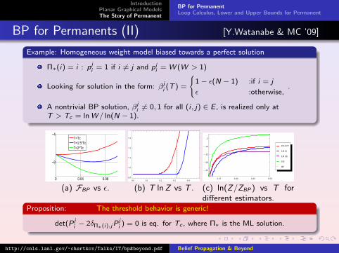
BP for Permanents (II) [Y.Watanabe & MC ’09]

Example: Homogeneous weight model biased towards a perfect solution

Π∗(i) = i : pji = 1 if i 6= j and pi

i = W (W > 1)

Looking for solution in the form: βji (T ) =

{1− ε(N − 1) :if i = j

ε :otherwise,.

A nontrivial BP solution, βji 6= 0, 1 for all (i , j) ∈ E , is realized only at

T > Tc = ln W / ln(N − 1).

0 0.04 0.08

−8

−4

T=TcT=1.5*TcT=2*Tc

(a) FBP vs ε.0.0 0.1 0.2 0.3 0.4

6.9

7.0

7.1

7.2

7.3

(b) T ln Z vs T .

0.35 0.40 0.45 0.50

-25

-20

-15

-10

-5

BP

UB

LB HIILLB HILEXACT

(c) ln(Z/ZBP) vs T fordifferent estimators.

Proposition: The threshold behavior is generic!

det(P ji − 2δΠ∗(i),jP

ji ) = 0 is eq. for Tc , where Π∗ is the ML solution.





Three faces of Loop Calculus for Permanent

Z = ZBP ∗ z, z ≡ 1 +∑

C rC , rC =(∏

i∈C (1− qi )) (∏

j∈C (1− qj ))∏

(i,j)∈Cβ

ji

1−βji

z = ∂2NZ(ρ1,··· ,ρN ,ρ1,··· ,ρN )

∂ρ1···∂ρN∂ρ1···∂ρN

∣∣∣∣ρ1=···=ρN =ρ1···=ρN =0

Z(ρ) ≡ exp(∑

i ρi +∑

j ρj)∏

(i,j)

(1 +

βji

(1−βji )

exp(−ρi − ρj

))

Main Theorem of [arxiv:0911.1419 Y. Watanabe & MC ’09]

Z = perm(P) = ZBP ∗ perm(β. ∗ (1− β))∏

(i,j)∈E (1− βji )−1

where β is the double-stochastic BP-solution matrix for P





Upper and Lower Bounds for Permanent [Y. Watanabe & MC ’09]

Gurvits (2008)-van der Waerden (1926) Theorem

For an arbitrary non-negative N × N matrix A, perm(A) ≥ cap(pA) NN

N!, where

pA(x) =∏

i

∑j ai,jxj , cap(pA) = infx∈RN

>0

pA(x)∏j xj

Application of the Gurvits-van der Waerden Theorem to the Loop Series yields

The low bound is invariant wrt BP transformation

perm(β. ∗ (1− β)) ≥ N!NN

∏(i,j)∈E (1− βj

i )βji

Another (dominating at high temperature) low bound on the Loop Series

perm(β. ∗ (1− β)) ≥ 2∏

i βΠ(i)i (1− βΠ(i)

i )

Upper Bound following from the Godzil-Gutman representation for permanent

perm(β. ∗ (1− β)) ≤∏

j (1−∑

i (βji )2)





Summary of the Permanent Story

Selling: arxiv:0911.1419

Threshold behavior of BP solution wrt temperature

New low and upper bounds for permanent based on LoopCalculus

Buying:

Improved Algorithm correcting permanent beyond BP

New Applications for the technique



Auxiliary Material for Planar & Surface

Example (1): Statistical Physics

Ising model σi = ±1

P(~σ) = Z−1 exp(∑

(i ,j) Jijσiσj

)Jij defines the graph (lattice)

Graphical Representation

Variables are usually associated with vertexes ... but transformation tothe Forney graph (variables on the edges) is straightforward

Ferromagnetic (Jij < 0), Anti-ferromagnetic (Jij > 0) and Frustrated/Glassy

Magnetization (order parameter) and Ground State

Thermodynamic Limit, N →∞Phase Transitions





Example (2): Information Theory, Machine Learning, etc

Probabilistic Reconstruction (Statistical Inference)

~σorig ⇒ ~x ⇒ ~σ

original

data~σorig ∈ Ccodeword

noisy channel

P(~x |~σ)

corrupted

data:

log-likelihood

magnetic field

statistical

inference

possible

preimage

~σ ∈ C

Maximum Likelihood [ground state]

Marginalization

ML(~x) = arg max~σP(~x |~σ) σ∗i (~x) = arg max

σi

∑~σ\σi

P(~x |~σ)

Counting (Partition Function): Z (~x) =∑

~σ P(~x |~σ)





Grassmann (fermion, nilpotent) Calculus for Pfaffians

Grassman (nilpotent) Variables on Vertexes

∀(a, b) ∈ Ge : θaθb + θbθa = 0

∫dθ = 0,

∫θdθ = 1

Pfaffian as a Gaussian Berezin Integral over the Fermions

∫exp

(−1

2~θtA~θ

)d~θ = Pf(A) =

√det(A)

Pfaffian Formula




Ice Model [vertexes of max degree 3]

#PL-3-NAE-ICE [Valiant ’02]

Input: A planar graph G = (V;E) of maximum degree 3.

Output: The number of orientations (arrows) such that no node has all theedges directed towards it or away from it.

From arrows to binary variables

Edge {a, b} is broken in two byinsertion of a− b vertex

Introduce binary variables s.t. ifa→ b ⇒ πa,a−b = 0, πb,a−b = 1b → a ⇒ πa,a−b = 1, πb,a−b = 0

Zice =∑π′

∏a∈G0

fa(πa)

∏{a,b}∈G1

ga−b(πa,a−b, πb,a−b)

fa(π′a) =

{1, ∃ b, c ∈ δG (a), s.t. πa,a−b 6= πa,a−c0, otherwise

ga−b(π′a) =

{1 πa,a−b 6= πb,a−b0, otherwise

Holographic Gadgets & Gauges




Ice Model [vertexes of max degree 3] II

General Gauge Transformation

fa(πa)→ fa(πa) =∑π′a

∏b∼a

Gab(πab, π′ab)

fa(π′a)

∀{a, b} ∈ G1 :∑π

Gab(π, π′)Gba(π, π′′) = δ(π′, π′′)

Z =∑π

∏a∈G0

fa(πa) =∑π

∏a∈G0

∑π′a

∏b∼a

Gab(πab, π′ab)

fa(πa)

Gauge Transformation for the Ice model

G(ice)a,a−b

=1√

2

(1 1−1 1

)ga−b(π′a) =

1, πa,a−b = πb,a−b = 0−1, πa,a−b = πb,a−b = 10, otherwise

fa(πa,a−1, πa,a−2, πa,a−3) =3√

2∗

1, πa,a−1 = πa,a−2 = πa,a−3 = 0−1/3,

∑i πa,a−i = 2

0, otherwise

Holographic Gadgets & Gauges



Auxiliary Material for Planar & SurfaceEdge-Binary Wick Models (of arbitrary degree)Kasteleyn Conjecture for Dimer Model on Surface Graphs

Edge Binary Wick (EBW) Models [Chernyak, MC ’09]

ZEBW (W ) =∑

γ={γab}∈Z1(G;Z2)

∑a∼b γab 6=0∏b∈G0

W(b){a1,··· ,a2k}≡{a|a∼b;γab=1}

and other 2‐vertex

and other 4‐vertex

• All odd weights are zero• Even (d > 2) weights are expressed

via pair-wise weights

W(b){a1,··· ,a2k}

≡∑

ξ∈P([2k−1])

W(b)ξ,a1···a2k

, W(b)ξ,a1···a2k

≡ (−1)

number of crossings (mod 2)︷︸︸︷p<p′∑

p,p′∈ξ

Cα(p) · Cα(p)′

·∏p∈ξ

W(b)α(p)

Examples of 6-colorings and extensions of a EBW-model 6 vertex

1 2

3

45

6

W16W25W34 [zero crossing]

1 2

3

45

6

−W12W35W46 [one crossing]

1 2

3

45

6

W13W25W46 [two crossings]

1 2

3

45

6

−W14W25W36 [three crossings]




Edge Binary Wick Models (II)

Known Easy Planar Graphical Models & EBW

∃ a gauge transformation reducing any easy planar model to a EBWDimer Model

Ising Model

Ice Model

Possibly all models discussed in the “holographic” papers

Any EBW model on a planar graph is EASY

Equivalent to Gaussian Grassman Models on the same graph

Partition function is Pfaffian of a |G1| × |G1| matrix




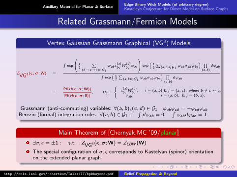
Related Grassmann/Fermion Models

Vertex Gaussian Grassmann Graphical (VG3) Models

ZVG3 (ς,σ; W) =

∫exp

12

∑(b→a→c)∈G1

ϕabς(a)bc

W(a)bcϕac

exp(

12

∑(a,b)∈G1

ϕabσabϕba

) ∏(a,b)

dϕab

∫exp(

12

∑(a,b)∈G1

ϕabσabϕba

) ∏(a,b)

dϕab

=Pf(H(ς,σ; W))

Pf(H(ς,σ; 0)), Hij =

{ς

(a)bc

W(a)bc, i = (a, b) & j = (a, c), where b 6= c ∼ a,

σab, i = (a, b), & j = (b, a).

Grassmann (anti-commuting) variables: ∀(a, b), (c, d) ∈ G1 ϕabϕcd = −ϕcdϕab

Berezin (formal) integration rules: ∀(a, b) ∈ G1 :∫

dϕab = 0,∫ϕabdϕab = 1

Main Theorem of [Chernyak,MC ’09/planar]

∃σ, ς = ±1 : s.t. ZVG3 (ς,σ; W) = ZEBW (W)

The special configuration of σ, ς corresponds to Kastelyan (spinor) orientationon the extended planar graph




Dimer Model on Surface Graphs (I)

Partition function of dimer model on a surface graph of genus g isexpressed in terms of a (±1)-weighted sum over 22g determinants= surface-easy

Kasteleyn ’63;’67 - non-constructive (??) conjecture

Gallucio, Loebl ’99 - first [combinatorial] proof

Cimasoni, Reshetikhin ’07 - topological proof and relation togauge fermion models

genus g = 0 genus g = 1 genus g = 2




Dimer Model on Surface Graphs (II)

Partition Function of Dimer Model, πij = 0, 1, on a surface graph G

Z (G; z) =∑ dimers

~π

∏(i ,j)∈Γ(zij)

πij

Theorem: (formulation of Cimasoni, Reshetikhin)

Z (G; z) = 12g

∑[s] Arf(qs

π0)εs(π0)︸︷︷︸

=±1; π0−independent; depends only on [s]

Pf(As(z))

π0 is a reference dimer configuration

s is a Kasteleyn orientation; [s] equivalence classes of the Kasteleyn orientations,22g of them

εs(π) = ±1 defines total signature of the dimer configuration π wrt theKasteleyn orientation s

qsπ0

(α) is a well-defined quadratic form associated with s, π0 and α is a closedcurve on G; Arf(qs

π0) is the Arf-invariant of the quadratic form.




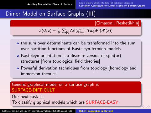
Dimer Model on Surface Graphs (III)

[Cimasoni, Reshetikhin]

Z (G; z) = 12g

∑[s] Arf(qs

π0)εs(π0)Pf(As(z))

the sum over determinants can be transformed into the sumover partition functions of Kasteleyn-fermion models

Kasteleyn orientation is a discrete version of spin(or)structures [from topological field theories]

Powerful derivation techniques from topology [homology andimmersion theories]

Generic graphical model on a surface graph isSURFACE-DIFFICULT

Our next task is:To classify graphical models which are SURFACE-EASY




Edge-Binary-Wick (EBW) Models andVertex Gaussian Grassman Graphical (VG3) modelson Surface Graphs

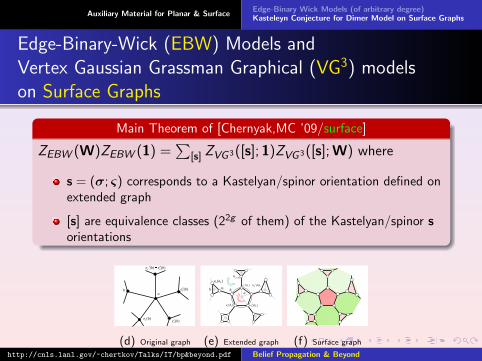
Main Theorem of [Chernyak,MC ’09/surface]

ZEBW (W)ZEBW (1) =∑

[s] ZVG3([s]; 1)ZVG3([s]; W) where

s = (σ; ς) corresponds to a Kastelyan/spinor orientation defined onextended graph

[s] are equivalence classes (22g of them) of the Kastelyan/spinor sorientations

a

)()( 41 bebe aa

b

)(bea )(2 bea

)(3 bea

(d) Original graph

baab

)( aa be

aaaa bebe ))(()( 11

a

)(2

aa be

)( bb ae

b

)(1 bea

a

(e) Extended graph (f) Surface graph




EBW and VG3 models on Surface Graphs (II)

ZEBW (W)ZEBW (1) =∑

[s] ZVG3([s]; 1)ZVG3([s]; W)

The multi-step proof of the main surface theorem includes

Extended/fat graph construction and partitioning ξ of the even generalized loopγ configurations into closed curves [Wick structure]

Analysis and relation between invariant objects (quadratic forms) for thegeneralized loops, [γ], and spinors, [s], defined on fat graphs and respectiveRiemann surfaces.

Term by term comparison of the relation between the partial ZEBW ([γ]; W) andZVG3 ([γ], [s]; W), where ZEBW (W) =

∑[γ] ZEBW ([γ]; W) and

ZVG3 ([s]; W) =∑

[γ] ZVG3 ([γ], [s]; W). This results in the system of 22g linear

equations for 22g unknowns ZEBW ([γ]; W).

Solving the linear equations we recover the main statement of the theorem.

2gZVG3 ([s]; 1) = Arf(q([s]))ZEBW (1), where q(s)(γ) = q([s])([γ]) is awell-defined quadratic form.




Main “take home” message

Q:

Describe the family of surface-easy edge-binary models on an arbitrarysurface graph G (partition function is reducible to a sum of 22g Pfaffians)

A: [constructive]

Generate an arbitrary Vertex Gaussian Grassmann binary-Gauge(VG3) Model on the graph

Fix the binary-gauge according to the Kasteleyn (spinor) rule on theextended graph

Construct respective Edge-Binary Wick model on the original graph

Apply an arbitrary skew-orthogonal (holographic)gauge/transformation

The partition function of the resulting model is the sum of 22g ±-weighted Pfaffians.

[All terms in the sum are explicitly known.]




Where do we go from here?

Future work

Use the described hierarchy of easy planar models as a basisfor efficient variational approximation of generic (difficult)planar problems. (The approach may also be useful forbuilding efficient variational matrix-product state wavefunctions for quantum models. Dynamical Bayesian Networks:1+1, tree+1, ....)

Study Wick Gaussian models on non-planar butPfaffian orientable or k-Pfaffian orientable graphs (where anydimer model on surface graph of genus g is 22g -Pfaffianorientable).

Almost Planar = Geographical Graphical Models,Renormalization Group, Generalized BP

Analogs of all of the above for Surface-Difficult Problems



@let@token Belief Propagation & Beyond

Documents

Transcript of @let@token Belief Propagation & Beyond