LETTERS - Smithsonian Institution
71
Transcript of LETTERS - Smithsonian Institution

LETTERSPUBLISHED ONLINE: 24 OCTOBER 2016 | DOI: 10.1038/NGEO2822
Climate, pCO2 and terrestrial carbon cycle linkagesduring late Palaeozoic glacial–interglacial cyclesIsabel P. Montañez1*†, Jennifer C. McElwain2*†, Christopher J. Poulsen3, Joseph D.White4,William A. DiMichele5, Jonathan P. Wilson6, Galen Griggs1 and Michael T. Hren7
Earth’s last icehouse, 300 million years ago, is considered thelongest-lived and most acute of the past half-billion years,characterized by expansive continental ice sheets1,2 and possi-bly tropical low-elevation glaciation3. This atypical climate haslong been attributed to anomalous radiative forcing promotedby a 3% lower incident solar luminosity4 and sustained lowatmospheric pCO2 (≤300ppm)5. Climate models6, however,indicateaCO2 sensitivityof ice-sheetdistributionandsea-levelresponse that questions this long-standing climate paradigmby revealing major discrepancy between hypothesized icedistribution,pCO2 , andgeologic recordsofglacioeustasy
2,6.Herewe present a high-resolution record of atmospheric pCO2 for16 million years of the late Palaeozoic, developed using soilcarbonate-based and fossil leaf-based proxies, that resolvesthe climate conundrum. Palaeo-fluctuations on the 105-yr scaleoccur within the CO2 range predicted for anthropogenic changeand co-varywith substantial change in sea level and ice volume.We further document coincidence between pCO2 changes andrepeated restructuring of Euramerican tropical forests that,in conjunction with modelled vegetation shifts, indicate amore dynamic carbon sequestration history than previouslyconsidered7,8 and a major role for terrestrial vegetation–CO2feedbacks indrivingeccentricity-scale climatecyclesof the latePalaeozoic icehouse.
Atmospheric pCO2 has generally declined over the past half-billionyears from highs of several 1,000 ppm, under which early metazoanlife radiated, to the lower concentrations characteristic of our pre-industrial glacial state. This trend was markedly disrupted in theCarboniferous–Permian (∼360 to 260million years ago (Ma)) by asustained period of low pCO2 and increasingly high pO2 attributed toradiation of the Earth’smost expansive tropical forests and attendantincreased organic matter burial in vast wetland habitats7,8. Theatypical surface conditions at this time, including anomalously lowradiative forcing possibly intensified by high pO2 (ref. 9), stronglyinfluenced the glaciation history and climate and ecosystemdynamics. Large-scale discrepancies, however, between modelledsurface conditions and those inferred from geologic recordschallenge existing climate paradigms and define new paradoxesregarding the climate dynamics of this palaeo-icehouse1–3,10.Atmospheric pCO2 estimates, central to resolving these issues, areinsufficiently resolved and poorly constrained5. Here we develop,for the late Palaeozoic, the first multi-proxy reconstruction of deep-time atmospheric CO2 at an unprecedented temporal resolution and
precision and compare our results with contemporaneous sea level,climate, and tropical vegetation records to assess linkages betweenclimate processes and the role of vegetation–climate feedbacks.
Palaeo-atmospheric pCO2 was reconstructed using soil-formedcarbonates and fossil-plant cuticles collected from a series oflong-eccentricity (405-kyr) cyclothems in the Illinois Basin,USA (Supplementary Table 1) making the independent CO2estimates directly comparable. Cyclothems, which archive glacial–interglacial cycles comparable to the Late Pleistocene11, providea chronostratigraphic framework for sampling palaeosols andplant-rich deposits at a 103- to 104-yr resolution (SupplementaryTable 1). Cross-Pangaean correlation of cyclothems enabled theintegration of fossil soils from the Appalachian, USA (n= 16) andDonets, Ukraine (n=4) basins with the Illinois Basin data (n=50).Pedogenic carbonate and organic matter δ13C values were appliedto the palaeosol CO2 palaeobarometer using the PBUQ model12to fully propagate uncertainty of input parameters and constrainestimated CO2 uncertainties (see Methods and SupplementaryTable 2). Intervals of high palaeosol diversity permitted evaluationof environmental influences on soil-water chemistry and carbonateδ13C. Two plant-based CO2 proxies, stomatal index (SI)13 and a
mechanistic stomatal model based on a universal leaf-gas-exchangeequation14, complement the mineral-based pCO2 estimates (seeMethods). Stomatal frequency and geometry of fossil leaf cuticlesand their δ13C were measured for two genera of long-rangingwetland seed ferns from 13 stratigraphic intervals (SupplementaryTable 3). Sampling of isotaphonomic plant-bearing intervalsminimized site- and time-specific environmental influences onstomatal and δ13C values.
Reconstructed CO2 (Fig. 1) varies between ∼200 and 700 ppmwith an apparent 105-yr rhythmicity. Notably, pCO2 estimatesobtained using all three proxies are in good agreement withvalues falling largely within the uncertainties. Generally, pCO2
falls below the modelled Carboniferous–Permian threshold forglacial inception (560 ppm)15 and well within the modelled rangefor sustainability of late Palaeozoic ice sheets6. A period mean of390 ppm ± 130 ppm (1σ ) is double that of existing estimates5,16and, considering the 3% lower solar luminosity, is more consistentwith the geologic record of ice distribution and magnitudesof glacioeustasy, thus resolving a long-standing data/modelmismatch in the behaviour of late Palaeozoic ice sheets2,3,6. LatePalaeozoic simulations6 predict dynamic change in ice-sheet sizeand distribution for the CO2 range over which our proxy estimates
© Macmillan Publishers Limited . All rights reserved
1Department of Earth and Planetary Sciences, University of California, Davis, California 95616, USA. 2Earth Institute, School of Biology and EnvironmentalScience, University College Dublin, Belfield, Dublin 4, Ireland. 3Department of Earth and Environmental Sciences, University of Michigan, Ann Arbor,Michigan 48109, USA. 4Department of Biology, Baylor University, Waco, Texas 76798, USA. 5Department of Paleobiology, Smithsonian Museum ofNatural History, Washington DC 20560, USA. 6Department of Biology, Haverford College, Haverford, Pennsylvania 19041, USA. 7Center forIntegrative Geosciences, University of Connecticut, Storrs, Connecticut 06269, USA. †These authors contributed equally to this work.*e-mail: [email protected]; [email protected]
824 NATURE GEOSCIENCE | VOL 9 | NOVEMBER 2016 | www.nature.com/naturegeoscience
NATURE GEOSCIENCE DOI: 10.1038/NGEO2822 LETTERS
100
302
303
304
305
306
307
308
StagesRu
ssia
nLa
te P
enns
ylva
nian
Mid
dle
Penn
sylv
ania
nG
zhel
ian
Virg
ilian
Kasi
mov
ian
Mos
covi
anD
esm
oine
sian
Mis
sour
ian
N. A
mer
.
200 300 400
Atmospheric CO2 (ppmv)
500 600 700
Empirical model:
Mechanistic model:N. ovata M. scheuchzeri
N. ovata
Pedogenic carbonate modelProtosols
M. scheuchzeri
800 900
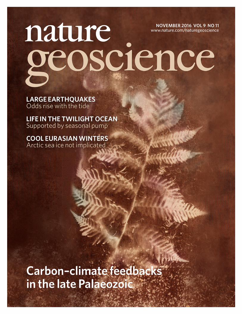
Figure 1 | Pennsylvanian pCO2 reconstructed using pedogenic carbonate-and fossil leaf-based proxies. The trendline connects average values ofmineral-based CO2 estimates per time increment (black filled circles);estimates from Protosols (open circles) are excluded. Grey shading andcoloured lines are the 16th and 84th percentile confidence intervals forpedogenic carbonate- and fossil plant-based CO2 estimates (indicated bygreen and orange), respectively. Cyclothem series are indicated byalternating blue/white banding (see Supplementary Information for agemodel). The lycopsid symbol indicates the timing of the MLPB ecologicturnover (∼305.9 Ma). N. ovata, Neuropteris ovata; M. scheuchzeri,Macroneuropteris scheuchzeri.
fluctuate, with ice distributed in multiple centres and of totalvolume that matches well with field-based reconstructions1,10.Moderate-size ice sheets, which form in simulations using pCO2
between 300 and 600 ppm, are far more sensitive to waxing andwaning than the largely unresponsive, coalesced ice sheets predictedunder previous CO2 estimates of <300 ppm, creating magnitudesof glacioeustasy more compatible with geologic records2.
Timescale (105-yr) and magnitude (200 to 300 ppm) of Pennsyl-vanian pCO2 fluctuations suggest eccentricity-scale variability withCO2 minima (160 to 300 ppm) comparable to Pleistocene glaciallevels17 but with higher maxima. For those cyclothems subject tohighest resolution sampling, CO2 concentrations rise rapidly early inthe cycle, falling to aminimum towards the top of each cycle (Fig. 1).Minimum calculated rates of CO2 rise (0.001 to 0.005 ppmyr−1) areconsistent with the lower range of rates for Pleistocene interglacials(0.003 to 0.02 ppmyr−1± 0.001 ppmyr−1)17.
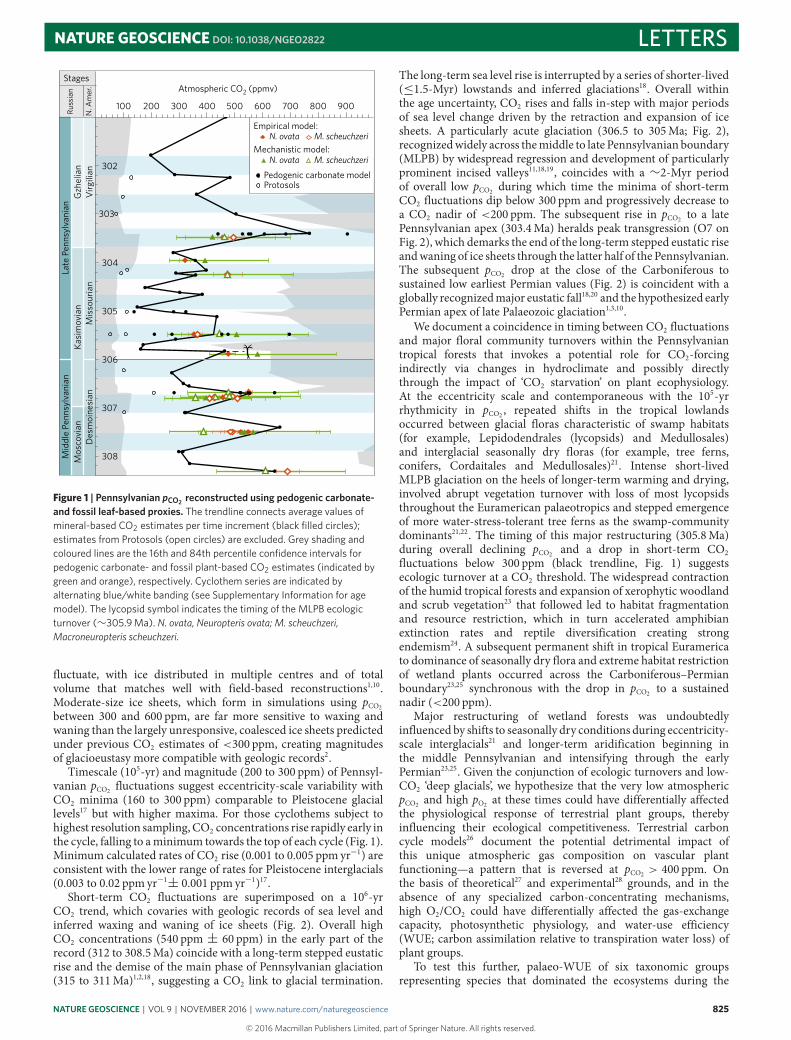
Short-term CO2 fluctuations are superimposed on a 106-yrCO2 trend, which covaries with geologic records of sea level andinferred waxing and waning of ice sheets (Fig. 2). Overall highCO2 concentrations (540 ppm ± 60 ppm) in the early part of therecord (312 to 308.5Ma) coincide with a long-term stepped eustaticrise and the demise of the main phase of Pennsylvanian glaciation(315 to 311Ma)1,2,18, suggesting a CO2 link to glacial termination.
The long-term sea level rise is interrupted by a series of shorter-lived(≤1.5-Myr) lowstands and inferred glaciations18. Overall withinthe age uncertainty, CO2 rises and falls in-step with major periodsof sea level change driven by the retraction and expansion of icesheets. A particularly acute glaciation (306.5 to 305Ma; Fig. 2),recognizedwidely across themiddle to late Pennsylvanian boundary(MLPB) by widespread regression and development of particularlyprominent incised valleys11,18,19, coincides with a ∼2-Myr periodof overall low pCO2 during which time the minima of short-termCO2 fluctuations dip below 300 ppm and progressively decrease toa CO2 nadir of <200 ppm. The subsequent rise in pCO2 to a latePennsylvanian apex (303.4Ma) heralds peak transgression (O7 onFig. 2), which demarks the end of the long-term stepped eustatic riseandwaning of ice sheets through the latter half of the Pennsylvanian.The subsequent pCO2 drop at the close of the Carboniferous tosustained low earliest Permian values (Fig. 2) is coincident with aglobally recognizedmajor eustatic fall18,20 and the hypothesized earlyPermian apex of late Palaeozoic glaciation1,3,10.
We document a coincidence in timing between CO2 fluctuationsand major floral community turnovers within the Pennsylvaniantropical forests that invokes a potential role for CO2-forcingindirectly via changes in hydroclimate and possibly directlythrough the impact of ‘CO2 starvation’ on plant ecophysiology.At the eccentricity scale and contemporaneous with the 105-yrrhythmicity in pCO2 , repeated shifts in the tropical lowlandsoccurred between glacial floras characteristic of swamp habitats(for example, Lepidodendrales (lycopsids) and Medullosales)and interglacial seasonally dry floras (for example, tree ferns,conifers, Cordaitales and Medullosales)21. Intense short-livedMLPB glaciation on the heels of longer-term warming and drying,involved abrupt vegetation turnover with loss of most lycopsidsthroughout the Euramerican palaeotropics and stepped emergenceof more water-stress-tolerant tree ferns as the swamp-communitydominants21,22. The timing of this major restructuring (305.8Ma)during overall declining pCO2 and a drop in short-term CO2fluctuations below 300 ppm (black trendline, Fig. 1) suggestsecologic turnover at a CO2 threshold. The widespread contractionof the humid tropical forests and expansion of xerophytic woodlandand scrub vegetation23 that followed led to habitat fragmentationand resource restriction, which in turn accelerated amphibianextinction rates and reptile diversification creating strongendemism24. A subsequent permanent shift in tropical Euramericato dominance of seasonally dry flora and extreme habitat restrictionof wetland plants occurred across the Carboniferous–Permianboundary23,25 synchronous with the drop in pCO2 to a sustainednadir (<200 ppm).
Major restructuring of wetland forests was undoubtedlyinfluenced by shifts to seasonally dry conditions during eccentricity-scale interglacials21 and longer-term aridification beginning inthe middle Pennsylvanian and intensifying through the earlyPermian23,25. Given the conjunction of ecologic turnovers and low-CO2 ‘deep glacials’, we hypothesize that the very low atmosphericpCO2 and high pO2 at these times could have differentially affectedthe physiological response of terrestrial plant groups, therebyinfluencing their ecological competitiveness. Terrestrial carboncycle models26 document the potential detrimental impact ofthis unique atmospheric gas composition on vascular plantfunctioning—a pattern that is reversed at pCO2 > 400 ppm. Onthe basis of theoretical27 and experimental28 grounds, and in theabsence of any specialized carbon-concentrating mechanisms,high O2/CO2 could have differentially affected the gas-exchangecapacity, photosynthetic physiology, and water-use efficiency(WUE; carbon assimilation relative to transpiration water loss) ofplant groups.
To test this further, palaeo-WUE of six taxonomic groupsrepresenting species that dominated the ecosystems during the
NATURE GEOSCIENCE | VOL 9 | NOVEMBER 2016 | www.nature.com/naturegeoscience
© Macmillan Publishers Limited . All rights reserved
825

LETTERS NATURE GEOSCIENCE DOI: 10.1038/NGEO2822
200296
Ma
297
298
299
300
301
302
303
304
305
306
307
308
309
310
311
296
Ma
297
298
299
300
301
302
303
304
305
IVFIVF
IVF
IVF
306
307
308
309
310
311
Mid
dle
Penn
sylv
ania
nLa
te P
enns
ylva
nian
Perm
ian
Russ
ian
Mid
-con
tinen
tcy
clot
hem
s
Don
ets
LSm
arke
r bed
sStages
N. A
mer
.M
osco
vian
Kasi
mov
ian
Mis
sour
ian
Gzh
elia
nV
irgili
anA
ssel
ian
Ass
elia
nD
esm
oine
sian
400
200 150 100 50 km
Atmospheric CO2 (ppmv)Donets Basin long-term
relative sea-levelonlap−offlap record
Onlap
5 pt running mean
Offlap
P5-0P4
P3
P2
P1
O7O6O5
O4-6H
O4-3HO4O2O1
N5-1N3-3
N3N2-HN1-6N1-3
N1
M9
M7M5M3M2M1L6L5
600
LOESS (0.1)
Bootstrapped errors:2.5% and 97.5%
CO2 estimates(this study)
CO2 estimates (revisedref. 30)
TopekaDeer Ck
LecomptonOreadCass
StantonIola
DeweyHogshooter
DennisSwopeHertha
Lost BranchAltamontPawnee
Upper Ft ScottLower Ft Scott
BevierVerdigris
800
Figure 2 | Consensus pCO2 curves defined by LOESS analysis of combined pedogenic carbonate- and fossil plant-based CO2 estimates. LOESS CO2estimates (black filled circles) include CO2 estimates (open blue circles) from ref. 30 revised using MatLab code PBUQ12 and improved input parameters.LOESS trend lines are 0.1 (black) and 0.3 (orange) smoothing. Donets Basin sea-level history18 was revised for the newest Carboniferous timescale; majorsea-level lowstands are intervals of o�ap beyond 100 km (dashed line). Interbasinal correlation of cyclothems is indicated by alternating blue and whiteintervals. Incised valley fill (IVF): location of ‘major’ incised valley fills recording the greatest extents of seaward withdrawal of the Midcontinent Sea11,19.The lycopsid symbol is as in Fig. 1. LS, Limestone.
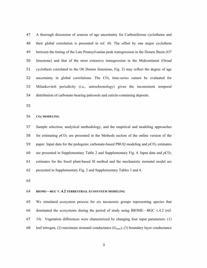
period of study were modelled using a terrestrial biospheremodel and Pennsylvanian–Permian O2/CO2 (Fig. 3a andsee Supplementary Information). WUE of fossil tree ferns(for example, Pecopteris) was consistently >5.5 times higher thancoeval Lepidodendrales, whereas Macroneouropteris and ‘otherMedullosales’ were minimally 2.5 to 3 times greater (Fig. 3b). The‘WUE advantage’ of Medullosales over Lepidodendrales increasedfurther when prevailing atmospheric CO2 decreased below 400 ppm(Fig. 3b), characteristic of the ‘deep palaeo-glacials’. Although theseecophysiological findings suggest that climatic/edaphic dryingwould have been ecologically disadvantageous to Lepidodendralesand Sphenophyllum compared with all other taxa across therange of estimated Pennsylvanian–Permian CO2 concentrations,they further strongly implicate the role of a low CO2-threshold(<400 ppm) as a driver of ecological turnovers.
Climate-driven vegetation changes had the potential to feedbackon CO2 through changes in terrestrial C sequestration given theexpanse and predominance of the tropical forests8 during glacials
and their dynamic compositional changes21,23. At the eccentricityscale, modelled biome distribution6 in response to orbitally drivenchanges in solar insolation and pCO2 indicates a large displacementin tropical vegetation (up to 7%) with shifts from wetland forests toseasonally dry flora during interglacials (Supplementary Table 9),a finding consistent with palaeobotanical records21. Estimatedconsequent changes in C sequestration potential are sufficient toincrease the CO2 flux to the atmosphere by 0.3 ppmyr−1± 0.2during interglacials and reduce it by a similar amount duringlonger-lived glacials. Even accounting for CO2 absorption by othersurface C sinks, the increased CO2 flux substantially outpacesminimum CO2 rise rates during deglaciation inferred from ourrecord, demonstrating the potential for tropical vegetation tomodulate late Palaeozoic pCO2 . Additionally, rapid tundra expansion(by up to 16%), coincident with solar insolation minima at theend of each interglacial, indicates a possible carbon sink of 0.02to 0.05 ppmyr−1, highlighting the potential role of high-latitudevegetation in promoting renewed ice buildup.
826
© Macmillan Publishers Limited . All rights reserved
NATURE GEOSCIENCE | VOL 9 | NOVEMBER 2016 | www.nature.com/naturegeoscience

NATURE GEOSCIENCE DOI: 10.1038/NGEO2822 LETTERS
0
10
20
30
40
50
60
70
80
90
Other Medullosales MacroneuropterisSphenophyllum LepidodendralesCordaitales Tree ferns
0
1
2
3
4
5
6
7
8
0 300 600 900 1,200 1,500 1,800CO2 (ppm)
WU
E ra
tioW
UE
(µm
ol C
O2 p
er m
mol
H2O
)
a
b
Figure 3 | Comparison of modelled water-use e�ciency (WUE) ofdominant Carboniferous taxa in relation to prevailing atmospheric pCO2
concentration. a,b, WUE values modelled using BIOME—BGC v.4.2 (seeSupplementary Information) (a), and expressed as a ratio to the WUEvalues of Lepidodendrales (b). Note that tree ferns consistently have WUEvalues that are higher than all other taxa and at minimum six times greaterthat those of Lepidodendrales, whereas the Macroneouropteris/Lepidodendrales WUE ratio shows an increasing trend with decliningatmospheric CO2.
This firstmulti-proxyCO2 record for the pre-Cenozoic illustratessubstantial fluctuation in palaeo-atmospheric pCO2 over a hierarchyof timescales during the only other Phanerozoic period of overalllow CO2. Notably, Pennsylvanian CO2 fluctuations, within therange anticipated for the twenty-first century, were associated withmajor changes in ice volume, sea level and repeated restructuringof the Earth’s most extensive tropical forests. In stark contrast tothe Late Pleistocene when the terrestrial organic carbon reservoirserved as a C sink during interglacials29, a net positive terrestrialC sink was established during late Palaeozoic glacials due tothe unprecedented geographic expanse and carbon sequestrationpotential of the palaeo-tropical wetland forests. Together, theresponse to climate change of the C sequestration potential oftropical and tundra biomes, extending over 35 to 50% of Pangaea,highlights the capacity of the terrestrial biosphere to drive C cycle
dynamics during Earth’s penultimate icehouse. Notably, the verylow pCO2 of the deep glacials raises an important yet unaddressedecologic issue as to whether selective ecophysiological stress at CO2thresholds contributed to major ecologic turnovers of the earliesttropical forests.
MethodsMethods, including statements of data availability and anyassociated accession codes and references, are available in theonline version of this paper.
Received 11 May 2016; accepted 7 September 2016;published online 24 October 2016
References1. Fielding, C. R. et al . Stratigraphic imprint of the Late Palaeozoic Ice Age in
eastern Australia: a record of alternating glacial and nonglacial climate regime.J. Geol. Soc. Lond. 165, 129–140 (2008).
2. Montañez, I. P. & Poulsen, C. J. The Late Paleozoic Ice Age: an evolvingparadigm. Annu. Rev. Earth Planet. Sci. 41, 629–656 (2013).
3. Soreghan, G. S., Sweet, D. E. & Heavens, N. G. Upland glaciation in tropicalPangaea: geologic evidence and implications for late Paleozoic climatemodeling. J. Geol. 122, 137–163 (2014).
4. Crowley, T. J. & Baum, S. K. Modeling late Paleozoic glaciation. Geology 20,507–510 (1992).
5. Royer, D. L. Treatise on Geochemistry 2nd edn, Vol. 6 (eds Holland, H. &Turekian, K.) 251–267 (Elsevier Ltd, 2014).
6. Horton, D. E., Poulsen, C. J. & Pollard, D. Influence of high-latitudevegetation feedbacks on late Palaeozoic glacial cycles. Nat. Geosci. 3,1–6 (2010).
7. Berner, R. A. The long-term carbon cycle, fossil fuels, and atmosphericcomposition. Nature 426, 323–326 (2003).
8. Cleal, C. J. & Thomas, B. A. Palaeozoic tropical rainforests and theireffect on global climates: is the past the key to the present? Geobiology 3,13–31 (2005).
9. Poulsen, C. J., Tabor, C. & White, J. D. Long-term climate forcing byatmospheric oxygen concentrations. Science 348, 1238–1241 (2015).
10. Isbell, J. et al . Glacial paradoxes during the late Paleozoic ice age: evaluatingthe equilibrium line altitude as a control on glaciation. Gondwana Res. 22,1–19 (2012).
11. Heckel, P. H. Pennsylvanian stratigraphy of Northern MidcontinentShelf and biostratigraphic correlation of cyclothems. Stratigraphy 10,3–39 (2013).
12. Breecker, D. O. Quantifying and understanding the uncertainty of atmosphericCO2 concentrations determined from calcic paleosols. Geochem. Geophys.Geosyst. 14, 3210–3220 (2013).
13. McElwain, J. C. & Chaloner, W. G. Stomatal density and index of fossilplants track atmospheric carbon dioxide in the palaeozoic. Ann. Bot. 76,389–395 (1995).
14. Franks, P. J. et al . New constraints on atmospheric CO2 concentration for thePhanerozoic. Geophys. Res. Lett. 41, 4685–4694 (2014).
15. Lowry, D. P., Poulsen, C. J., Horton, D. E., Torsvik, T. H. & Pollard, D. Controlson Paleozoic ice sheet initiation. Geology 42, 627–630 (2014).
16. Breecker, D. O., Sharp, Z. D. & McFadden, L. D. Atmospheric CO2
concentrations during ancient greenhouse climates were similar to thosepredicted for A.D. 2100. Proc. Natl Acad. Sci. USA 107, 576–580 (2010).
17. Siegenthaler, U. et al . Stable carbon cycle-climate relationship during the LatePleistocene. Science 310, 1313–1317 (2005).
18. Eros, J. M. et al . Sequence stratigraphy and onlap history, Donets Basin,Ukraine: Insight into Late Paleozoic ice age dynamics. Palaeogeogr.Palaeoclimatol. Palaeoecol. 313, 1–25 (2012).
19. Belt, E. S., Heckel, P. H., Lentz, L. J., Bragonier, W. A. & Lyons, T. W. Record ofglacial-eustatic sea-level fluctuations in complex middle to late Pennsylvanianfacies in the Northern Appalachian Basin and relation to similar events in theMidcontinent basin. Sediment. Geol. 238, 79–100 (2011).
20. Koch, J. T. & Frank, T. D. The Pennsylvanian-Permian transition in thelow-latitude carbonate record and the onset of major Gondwanan glaciation.Palaeogeogr. Palaeoclimatol. Palaeoecol. 308, 362–372 (2011).
21. DiMichele, W. A. Wetland-dryland vegetational dynamics in the Pennsylvanianice age tropics. Int. J. Plant Sci. 175, 123–164 (2014).
22. Phillips, T. L. & Peppers, R. A. Changing patterns of Pennsylvanian coal-swampvegetation and implications of climatic control on coal occurrence. Int. J. CoalGeol. 3, 205–255 (1984).
NATURE GEOSCIENCE | VOL 9 | NOVEMBER 2016 | www.nature.com/naturegeoscience
© Macmillan Publishers Limited . All rights reserved
827

LETTERS NATURE GEOSCIENCE DOI: 10.1038/NGEO2822
23. DiMichele, W. A., Montañez, I. P., Poulsen, C. J. & Tabor, N. J.Vegetation-climate feedbacks and regime shifts in the Late Paleozoic ice ageearth. Geobiology 7, 200–226 (2009).
24. Sahey, S., Benton, M. J. & Falcon-Lang, H. J. Rainforest collapse triggeredcarboniferous tetrapod diversification in Euramerica. Geology 38,1079–1082 (2010).
25. Tabor, N. J., DiMichele, W. A., Montañez, I. P. & Chaney, D. S. Late Paleozoiccontinental warming of a cold tropical basin and floristic change in westernPangea. Int. J. Coal Geol. 119, 177–186 (2013).
26. Beerling, D. J. & Berner, R. A. Impact of a Permo-Carboniferous high O2
event on the terrestrial carbon cycle. Proc. Natl Acad. Sci. USA 97,12428–12432 (2000).
27. Flexas, J. Mesophyll diffusion conductance to CO2: an unappreciated centralplayer in photosynthesis. Plant Sci. 193, 70–84 (2012).
28. McElwain, J. C., Yiotis, C. & Lawson, T. Using modern plant trait relationshipsbetween observed and theoretical maximum stomatal conductance and veindensity to examine patterns of plant macroevolution. New Phytol. 209,94–103 (2015).
29. Adams, J. M., Faure, H., Faure-Denard, L., McGlade, J. M. &Woodward, F. I.Increases in terrestrial carbon storage from the Last Glacial Maximum to thepresent. Nature 348, 711–714 (1990).
30. Montañez, I. P. et al . CO2-forced climate instability and linkages to tropicalvegetation during late paleozoic deglaciation. Science 315, 87–91 (2007).
AcknowledgementsWe thank D. Breecker for discussion and comments on this work, and R. Barclay,J. Antognini, D. Garello, A. Byrd, R. Chen, C. Marquardt and D. Rauh for assistancein the research, D. Horton for access to palaeoclimate model results, and N. Taborfor a subset of stable isotopic analyses. This work was funded by NSF grantsEAR-1338281 (I.P.M.), EAR-1338200 (C.J.P.), EAR-1338247 (J.D.W.), and EAR-1338256(M.T.H.), and ERC-2011-StG and 279962-OXYEVOL to J.C.M.
Author contributionsI.P.M. and J.C.M. devised and carried out the CO2 proxy reconstruction and J.D.W.,W.A.D., J.P.W. and M.T.H. contributed to the parameterization and sensitivity analyses ofthe palaeo-CO2 models. C.J.P. undertook the climate modelling analysis, J.D.W. thebiogeochemical ecosystem modelling, and G.G. contributed to the CO2 modelling. Allauthors contributed to the development of ideas, data interpretation, and writing ofthe manuscript.
Additional informationSupplementary information is available in the online version of the paper. Reprints andpermissions information is available online at www.nature.com/reprints.Correspondence and requests for materials should be addressed to I.P.M. or J.C.M.
Competing financial interestsThe authors declare no competing financial interests.
828
© Macmillan Publishers Limited . All rights reserved
NATURE GEOSCIENCE | VOL 9 | NOVEMBER 2016 | www.nature.com/naturegeoscience

NATURE GEOSCIENCE DOI: 10.1038/NGEO2822 LETTERSMethodsSamples. Calcite nodules and rhizolith samples (n=304) were collected fromPennsylvanian-age cyclothemic successions from: Illinois Basin surface andsubsurface mines and five cores, housed at the Prairie Research Institute, IllinoisState Geological Survey; and outcrops in the Appalachian Basin, USA and DonetsBasin, Ukraine (Supplementary Table 2). Fossil pteridosperm leaves were extractedfrom samples obtained from the Department of Paleobiology, National Museum ofNatural History, Smithsonian Institution (Supplementary Table 3). For outcrops,profiles were trenched to ensure a fresh exposure; samples were collected from atleast 0.5m beneath the surfaces of mature and immature (Protosols) palaeosols.Palaeosols were classified on the basis of macro- and micromorphologic featuresusing the scheme of ref. 31. Cuticles of individual pinnules were isolated frombedding plane surfaces either by the non-destructive (polyester peels) technique ofref. 32 or by bulk maceration.
Geochemical methodology. Pedogenic carbonate samples were thick-sectioned(∼200 µm thick) and evaluated for evidence of recrystallization or diageneticcements using transmitted and cathodoluminescent light (see ref. 33). Micriticcalcite exhibiting pedogenic micromorphologies was microsampled using aMerchantek automated microsampler. Approximately 50 µg of carbonate wasroasted at 375 ◦C under vacuum for 2 h to remove organics and subsequentlyreacted in 105% phosphoric acid at 90 ◦C in a common acid bath of a GVI OptimaIRMS in the Stan Margolis Stable Isotope Laboratory, University of California,Davis (UCD). External precision for δ13C measurements based on standards andreplicates was>±0.04h.
Organic matter C isotopic data were obtained from: coal vitrinite macerals anddiscrete fossil plant matter in mudstones closely associated with palaeosols; and/orfrom organic matter occluded within pedogenic nodules. For CO2 estimates madeusing the mechanistic model of ref.14, the δ13C of fossil leaf cuticles, which wereused for stomatal-index-based CO2 estimates, was measured. The δ13C values of allmaterials are presented in Supplementary Tables 2 and 3.
For coals and sediment-associated organic matter, samples were rinsed in 1 NHCl overnight at room temperature and washed four times with nanopure H2O toremove any carbonate and hydrolysable C. Between one hundred and two hundredmicrograms of cleaned and dried organic matter or fossil cuticle, previouslycleaned to remove mineral matter, were loaded in tin capsules. C isotope analysis ofcoals, discrete fossil plant matter, and fossil cuticles was carried out on a PDZEuropa elemental analyser interfaced to a PDZ Europa 20-20 IRMS at the StableIsotope Facility, UCD. External precision for the δ13C measurements based onrepeated analysis of standards is better than±0.3h. Additionally, the δ13C valuesof organic matter occluded within pedogenic carbonates (n=22) were measuredfor 18 stratigraphic intervals. Organic matter was isolated from 10 to 20mg ofpulverized carbonate through repeated rinsing with 1 N HCl and subsequentlywashed with nanopure H2O to remove all carbonate. Dry residues were processedoffline and analysed by IRMS in the UC Davis Stable Isotope Laboratory or in theStable Isotope Laboratory, Southern Methodist University (courtesy of N. Tabor).External precision for the δ13C measurements is≤±0.3h.
Input parameters for palaeosol barometer model and uncertainty estimates. TheMatLab code PBUQ12 was used to estimate palaeo-CO2. PBUQ uses the palaeosolcarbonate CO2 palaeobarometer equation34 and Monte Carlo error propagation todefine a distribution of CO2 from which mean, median and percentile (16th and84th) values are calculated. Individual input data for the PBUQ model (n=81)consist of average measured values from either: an individual palaeosol of a givensoil order (that is, a sample); or a series of stacked palaeosols of the same soil orderfrom within one stratigraphic interval (that is, a sample set). Palaeosols of the sameage but of differing soil order were modelled individually resulting in multipleestimates for over 60% of the time slices. Input parameters for PBUQ werecalculated as follows and are presented in Supplementary Table 2.
Temperature. PBUQ uses, as a default, palaeo-MAAT to calculate the temperatureof soil carbonate formation based on a transfer function (Y=0.506∗X+17.974,where Y is the carbonate formation temperature and X is MAAT)12. For the subsetof new samples (n=70) of Pennsylvanian through earliest Permian age, weassigned a constant MAAT range (23 ◦C± 3 ◦C) that spans the minimum tomaximum temperatures modelled for the late Palaeozoic continental tropics over apCO2 of 280 to 840 ppm (refs 2,6). This approach conservatively represents latePalaeozoic MAATs in the palaeotropics. The temperature range utilized in thisstudy (20 to 26 ◦C) overlaps with the lower range of soil temperatures (22 to 32 ◦C)inferred from pedogenic minerals35 for four of the same stratigraphic intervals inthe Illinois Basin, thus providing confidence that a MAAT range of 20 to 26 ◦C isreasonable. Proxy soil temperatures could be several degrees to possibly 10 ◦Chigher than warm-season surface air temperatures during the Pennsylvanian andearly Permian given the influence of surface latent and sensible heat fluxes on soiltemperatures36,37. Notably, if the MAAT values used in this study are too low (thatis, if surface air temperatures in the tropics averaged annually over 26 ◦C) then the
CO2 estimates during peak intervals shown on Figs 1 and 2 are underestimated andthe magnitudes of change within the 105-yr fluctuations are minimum ranges.Comparison of CO2 estimates made using the same parameterization of PBUQ butwith a temperature of 32 ◦C± 3 ◦C indicates an average difference of 42.4 ppmbetween the higher temperature estimates and those made using 23◦ C± 3 ◦C anda standard deviation of the variance of± 147.3 ppm. These values fall within theuncertainty of modelled pCO2 .
For the modelling of previously published30 latest Pennsylvanian to earlyPermian sample sets (n=11), we constrained MAATs using proxy soiltemperatures25, which were derived from many of the same palaeosols (∼50%)used in this study. See Supplementary Table 2 for specifics of how MAATs wereconstrained for this subset of samples.
Total soil CO2δ13C. The average (±2 standard error (s.e.)) δ13C values of
pedogenic carbonates from a given palaeosol or series of palaeosols was used as aproxy for the δ13C value of total soil CO2. We consider measured pedogeniccarbonate δ13C values to be a robust proxy of soil-water CO2 during formationgiven the lack of evidence for mineral recrystallization and overgrowth and themoderate burial thermal histories of the Illinois Basin35.
Respired δ13C. PBUQ permits four options for defining the δ13C value of therespired CO2 contribution to the soil. This study utilized two of these options. Thefirst proxy of respired CO2δ
13C is the average (±2 s.e.) measured δ13C of coalmacerals and fossil plant matter extracted from mudstones most stratigraphicallyproximal to the carbonate-bearing palaeosols. In the cyclothemic successions of theIllinois, Appalachian and Donets basins, coals and/or plant-rich mudstonestypically overlie palaeosols; thus, the organic matter is considered representative ofthe organic-rich surface A horizon of these palaeosols. The second proxy of respiredCO2δ
13C is the measured δ13C value of organic matter occluded within pedogeniccarbonates, which formed in the B horizon of palaeosols. For those soils for whichCO2 estimates were obtained using both proxies of respired CO2δ
13C, pCO2
estimates shown on Figs 1 and 2 are those made using occluded organic matter.This choice reflects that organic matter occluded in the pedogenic carbonates mostclosely approximates that of the soil in which the carbonate formed. CO2 estimatesfor both proxies of soil-respired CO2δ
13C are provided in Supplementary Table 2.PBUQ makes a correction to the input δ13Corg values of+0.5h for organic
matter that formed in the A horizon and of−1h for that formed in the B horizon.This correction is to account for the contribution in the carbonate-forming horizonof respired CO2 from A and B horizons of which the former is 12C-enriched relativeto the latter. In this study, although the δ13C values of the coal macerals arerepresentative of the A horizon, a+0.5h correction was not applied to coal δ13Corg
values given processes that can lead to 13C-enrichment in coal relative to soilorganic matter in the A horizon. The δ13C of coals rich in macerals derived fromwoody tissues (vitrinite) are 13C-enriched (∼2h) relative to macerals derived fromlipid-rich precursor material (liptinites)38. Therefore, the respired CO2 in the Ahorizon of palaeosols, which would have been dominated by respiration of leafmaterial and other less refractory organic matter, was probably 13C-depletedrelative to the organic matter contained in vitrinite-rich coals; thus, the correctionis effectively already accounted for. Moreover, coal δ13C typically increases duringcoalification resulting in values up to∼1h higher than contemporaneous C3-typeterrestrial plants38. Additionally, no correction was made to the input δ13Corg valuesof occluded organic matter, which formed in the B horizon, given that occludedorganic matter δ13C values measured in this study were similar to, to slightly morenegative than, those of contemporaneous coal or fossil plant matter.
Atmospheric δ13C. The best estimates of marine δ13Ccalcite (±1σ ) from a globalcompilation of Permo-Carboniferous brachiopods39 were input to PBUQ, fromwhich δ13Catm is calculated using the input temperatures and thetemperature-sensitive εcalcite−CO2(g) equation of ref. 40.
Soil-respired CO2, S(z). The soil-order specific ranges of soil-respired CO2
concentration (S(z)), which were defined on a set of 130 Holocenecarbonate-bearing palaeosols41, and modified in ref. 12, were used in thePBUQ modelling.
Reported pCO2 estimates (Supplementary Table 2) are presented as interquartilemean values rather than the default median values given that the truncated mean isa robust estimator of centrality for mixed distributions and the skewed S(z) inputdata set. A full discussion of this statistical approach and comparison of the medianand interquartile mean values of best estimates of late Palaeozoic pCO2 are presentedin the Supplementary Information and Supplementary Fig. 4.
Fossil cuticle-based CO2 estimates. Palaeo-atmospheric pCO2 was furtherestimated using two long-ranging and isotaphonomic, wetland pteridosperms(Neuropteris ovata andMacroneuropteris scheuchzeri) applied to the SI method anda mechanistic stomatal model of pCO2 . Measured input parameters for both proxymethods and the resulting pCO2 estimates are presented in Supplementary Table 3.
NATURE GEOSCIENCE | www.nature.com/naturegeoscience
© Macmillan Publishers Limited . All rights reserved

LETTERS NATURE GEOSCIENCE DOI: 10.1038/NGEO2822
Stomatal index method. The stomatal density and index of abaxial cuticles weremeasured on macrofossil cuticle specimens (peels) or on fragments obtainedthrough bulk maceration. A strong inverse relationship between stomatal density(SD) or SI and atmospheric CO2 concentration has been documented in living andextant plants13,42,43. Comparison of SI estimates and temporal trends betweencoexisting extant and extinct plants further demonstrates the robustness of thisCO2 proxy44,45. SD, the number of stomata per square millimetre area, and SI, thepercentage of leaf epidermal cells that are stomatal, were measured usingepifluorescent microscopy and a Leica ‘stacked image’ capture and analysis system.Between 4 and 10 regions (0.04mm2) were counted for each cuticle/leaf fragmentto define mean values per leaf (see ref. 44). We use the SI measurements as proxiesof palaeoatmospheric CO2 given that SI is generally considered a better metric ofchanges in atmospheric CO2 because it is less affected by environmental conditionsthan SD42,46. As some studies have suggested that SI can be impacted byenvironmental factors other than pCO2 (for example, irradiance, nutritionalconstraints47,48), we characterized, for leaf fragments of individual plants, thenatural intra- and inter-pinnule variability in stomatal traits.
SI values of medullosan (seed fern) cuticles from 13 Pennsylvanian cyclothems(Illinois Basin) indicate a lack of species specificity and an intra- and inter-pinnulevariability within individual plant beds (0.4 to 1.6, respectively) that is much lessthan the temporal variability (Supplementary Fig. 2). Within the limits of the datadistribution, both taxa and the variants define similar temporal shifts in SI that arebeyond the natural intra- and inter-pinnule and geographic variability. We interpretthe similar temporal changes in SI indicated by all taxa to record an atmosphericCO2 driver to the long-term genotypic response of SI in these Pennsylvanian plants.
SI values were calibrated to palaeo-pCO2 for a given time increment using thenearest-living equivalent (NLE) method of ref. 49, as applied to tree ferns50, and thestomatal ratio method13. Two extant tree ferns in the Order Cyatheales(Cyathea cooperii: SI=18.0; Dicksonia antarctica: SI= 20) and one tree-fern-likefern (Todea barbara (Osmundales): SI= 16.2) were selected as potential NLEspecies (NLEs) for the taxa Neuropteris andMacroneuropteris. Selection was basedon similarities in overall vegetative and ecological traits, which determineecophysiological processes, rather than reproductive traits, which differ betweenferns and seed ferns. The traits used included pinnae and pinnule macro- andmicromorphology and ecological traits such as canopy position and relativeabundance within palaeo- and modern forest communities (all understory,typically sub-dominant but can be dominant). An average SI value for the threeNLEs of 18.07 was used to calculate the stomatal ratio (NLE SI/Fossil SI) fromwhich CO2 concentration was estimated using the recent standardizationaccording to the formula of ref. 13 below:
Palaeo-pCO2 (ppm)= ((SINLEs=18.066)/SIfossil)
×360ppm [Recent standardization]
The Carboniferous standardization of ref. 49, frequently used to estimatemaximum CO2, was not used here because it assumes that geochemical massbalance model estimates of pCO2 for the Carboniferous are correct and anchorssubsequent stomatal ratio-based CO2 estimates to this Carboniferous calibrationpoint. Such an approach would not be valid here where we aim to quantifyCarboniferous CO2 independently of any model-based estimates.
Mechanistic model. The measured stomatal traits (density and guard cell lengthand width) and cuticle δ13C values of the two seed fern taxa used in this study wereapplied to the mechanistic stomatal model of ref. 14. This approach based on theuniversal leaf-gas-exchange equation, equates atmospheric CO2 with CO2
assimilation rate (An), which is prescribed at the taxonomic level; total stomatalconductance of the leaf, which is inferred from fossil cuticle stomatal traits; and thedifference in concentration of CO2 between the atmosphere and in the leaf (Ci/Caratio). Scaling factors used in the mechanistic model are a combination ofmeasured and inferred values (Supplementary Table 4). In this study, the stomataltraits (density and guard cell length) of the abaxial surface of the cuticles weremeasured on epifluorescent ‘stacked image’ photographs of cuticle/leaf fragmentsto define mean values per leaf. Only the abaxial cuticle surface was measured asthese seed fern taxa were hypostomatous.
CO2 estimates made using this mechanistic model are sensitive to the inputparameters of photosynthetic rate (Ao), defined in ref. 14 as that under currentambient CO2 conditions (400 ppm), and total operational conductance to CO2
diffusion from the atmosphere to sites of photosynthesis in the leaf (gc(tot)). Notably,CO2 estimates vary by several hundreds of parts per million depending on whichvalues are prescribed51. Ref. 14 suggest a photosynthetic rate (Ao) for all seed ferns(pteridosperms, including medullosans) of 6 µmol CO2 m−2 s−1 using a moderngymnosperm NLE. On the basis of all other physiological traits of thesemedullosans (high xylem conductivity, high gmax, relatively high vein density, thincuticle and broad, thin leaves), an angiosperm or tropical fern model is deemedmore appropriate46. Thus, Ao values (µmolm−2 s−1) for the two seed ferns studied
were estimated using three approaches: the scaling relationship between veindensity (Dv) and Ao for a range of angiosperm and fern taxa from refs 28,52);estimated Kleaf using measurements of mesophyll path length compared with amodern data set of ref. 53; and ecosystem model constraints (BIOME-BGC v.4.2)54on canopy average and maximum sunlit canopy CO2 assimilation under 400 ppmand the range of hypothesized late Palaeozoic pO2 . The methodology for these threeapproaches and results are presented in refs 51,55.
Total operational conductance (gc(tot)) is based on leaf boundary layerconductance (gcb) to CO2, the mesophyll conductance (gm), and operationalstomatal conductance (gc(op)). The suggested values of ref. 14 were used for gcb andgm. Ref. 14 recommends a scaling factor a 0.2 from maximum conductance to CO2
(gc(max)) to gc(op). This scaling relationship, however, is inversely correlated with CO2
(ref. 56). Both ref. 56 and ref. 28 observe a slightly higher scaling relationship forgc(op)/gc(max)of 0.25 and 0.3 respectively. Neuropteris andMacroneuropteris occupiedecological habitats with high water availability and could potentially have achieved40% of gc(max) values (0.4 scaling). A sensitivity analysis of values ranging from 0.2to 0.4 was undertaken to account for varying water supply rates to leaf tissue andsite water availability and thus uncertainty in this parameter51 but the mostconservative value of 0.2 was used here.
Details regarding the age (Supplementary Table 1) and geologic(Supplementary Fig. 9) models used in this study, statistical analysis of the pCO2
estimates, the terrestrial ecosystem modelling (BIOME-BGC v.4.2), and theterrestrial carbon sequestration calculations and associated discussion arepresented in the Supplementary Information.
Code availability. The code used to generate the pedogenic carbonate-based pCO2
estimates can be assessed in ref. 12. The code used to generate the mechanisticstomatal-based pCO2 estimates can be assessed in ref. 14. The code for the terrestrialbiosphere modelling can be downloaded free of charge at http://www.ntsg.umt.edu/project/biome-bgc. The GENESIS Earth system climate model, v. 3.0, coupled todynamic ecosystem and ice-sheet modelling components was used to generate themodelled vegetation data in Supplementary Table 9 (refs 57–59).
Data availability. All data supporting the findings of this study are available in theSupplementary Information files. Any additional information regarding this studyis available from the corresponding author on request.
References31. Mack, G. H., James, W. C. & Monger, H. C. Classification of paleosols. Geol.
Soc. Am. Bull. 105, 129–136 (1993).32. Kouwenberg, L. L. R., Hines, R. R. & McElwain, J. C. A new transfer technique
to extract and process thin and fragmented fossil cuticle using polyesteroverlays. Rev. Palaeobot. Palynol. 145, 243–248 (2007).
33. Deutz, P., Montañez, I. P. & Monger, H. C. Morphologies and stable andradiogenic isotope compositions of pedogenic carbonates in Late Quaternaryrelict and buried soils, New Mexico: an integrated record of pedogenicoverprinting. J. Sediment. Res. 72, 809–822 (2002).
34. Cerling, T. E. Use of carbon isotopes in paleosols as an indicator of the pCO2 ofthe paleoatmosphere. Glob. Geochem. Cycles 6, 307–314 (1992).
35. Rosenau, N. A. & Tabor, N. J. Oxygen and hydrogen isotope compositions ofpaleosol phyllosilicates: differential burial histories and determination ofmiddle-late Pennsylvanian low-latitude terrestrial paleotemperatures.Palaeogeol. Palaeoclimatol. Palaeoecol. 392, 382–397 (2013).
36. Passey, B. H., Levin, N. E., Cerling, T. E., Brown, F. H. & Eiler, J. M.High-temperature environments of human evolution in East Africa based onbond-ordering in paleosol carbonates. Proc. Natl Acad. Sci. USA 107,11245–11249 (2010).
37. Quade, J., Eiler, J., Daeron, M. & Achyuthan, H. The clumped isotopegeothermometer in soil and paleosol carbonate. Geochim. Cosmochim. Acta105, 92–107 (2013).
38. Rimmer, S. M., Rowe, H. D., Taulbee, D. N. & Hower, J. C. Influence of maceralcontent on δ13C and δ15N in a Middle Pennsylvanian coal. Chem. Geol. 77,77–90 (2006).
39. Grossman, E. L. et al . Glaciation, aridification, and carbon sequestration in thePermo-Carboniferous: the isotopic record from low latitudes. Palaeogeogr.Palaeoclimatol. Palaeoecol. 268, 222–233 (2008).
40. Romanek, C. S., Grossman, E. L. & Morse, J. W. Carbon isotopic fractionationin synthetic aragonite and calcite: effects of temperature and precipitation rate.Geochim. Cosmochim. Acta 56, 419–430 (1992).
41. Montañez, I. P. Modern soil system constraints on reconstructing deep-timeatmospheric CO2. Geochim. Cosmochim. Acta 101, 57–75 (2013).
42. Woodward, F. I. Plant-responses to past concentrations of CO2. Vegetation 104,145–155 (1993).
43. Kurschner, W. M., van der Burgh, J., Visscher, H. & Dilcher, D. L. Oak leaves asbiosensors of late Neogene and early Pleistocene paleoatmospheric CO2
concentrations.Mar. Micropaleontol. 27, 299–312 (1996).
© Macmillan Publishers Limited . All rights reserved
NATURE GEOSCIENCE | www.nature.com/naturegeoscience

NATURE GEOSCIENCE DOI: 10.1038/NGEO2822 LETTERS44. Barclay, R. S., McElwain, J. C. & Sageman, B. B. Carbon sequestration activated
by a volcanic CO2 pulse during oceanic anoxic event 2. Nat. Geosci. 3,205–208 (2010).
45. Steinthorsdottir, M., Jeram, A. J. & McElwain, J. C. Extremely elevated CO2
concentrations at the Triassic/Jurassic boundary. Palaeogeogr. Palaeoclimatol.Palaeoecol. 308, 418–432 (2011).
46. McElwain, J. C., Beerling, D. J. & Woodward, F. I. Fossil plants and globalwarming at the Triassic-Jurassic boundary. Science 28, 1386–1390 (1999).
47. Atchison, J. M., Head, L. M. & McCarthy, L. P. Stomatal parameters andatmospheric change since 7500 years before present: evidence from Eremophiladeserti (Myoporaceae) leaves from the Flinders Ranges region, South Australia.Aust. J. Bot. 48, 223–232 (2000).
48. Beerling, D. J., Fox, A. & Anderson, C. W. Quantitative uncertainty analyses ofancient atmospheric CO2 estimates from fossil leaves. Am. J. Sci. 309,775–787 (2009).
49. McElwain, J. C. & Chaloner, W. G. The fossil cuticle as skeletal record ofenvironmental change. Palaios 11, 376–388 (1996).
50. Steinthorsdottir, M. Atmospheric CO2 and Stomatal Responses at theTriassic-Jurassic Boundary PhD thesis, Univ. College Dublin (2010).
51. McElwain, J. C., Montañez, I. P., White, J. D., Wilson, J. & Yiotis, H. Wasatmospheric CO2 capped at 1000 ppm over the past 300 million years?Palaeogeogr. Palaeoclimatol. Palaeoecol. 441, 653–658 (2016).
52. Boyce, C. K. & Zwieniecki, M. A. Leaf fossil record suggests limited influence ofatmospheric CO2 on terrestrial productivity prior to angiosperm evolution.Proc. Natl Acad. Sci. USA 109, 10403–10408 (2012).
53. Brodribb, T. J., Feild, T. S. & Jordan, G. J. Leaf maximum photosynthetic rateand venation are linked by hydraulics. Plant Physiol. 144, 1890–1898 (2007).
54. White, M. A., Thornton, P. E., Running, S. W. & Nemani, R. R. Parameterizationand sensitivity analysis of the BIOME–BGC terrestrial ecosystem model: netprimary production controls. Earth Interact. 4, 1–85 (2000).
55. Wilson, J. P. et al . Earth-life transitions: paleobiology in the context ofEarth system evolution. Paleontological Society Paper 21 167–195(Yale Press, 2015).
56. Dow, G. J., Bergmann, D. C. & Berry, J. A. An integrated model of stomataldevelopment and leaf physiology. New Phytol. 201, 1218–1226 (2014).
57. Pollard, D. & Thompson, S.L. Use of a land-surface-transfer scheme (Lsx) in aglobal climate model—the response to doubling stomatal-resistance. GlobalPlanet Change 10, 129–161 (1995).
58. Thompson, S.L. & Pollard, D. A global climate model (genesis) with a land-surface transfer scheme (Lsx).1. Present climate simulation. J. Clim. 8,732–761 (1995).
59. Thompson, S.L. & Pollard, D. Greenland and Antarctic mass balances forpresent and doubled atmospheric CO2 from the GENESIS version-2 globalclimate model. J. Clim. 10, 871–900 (1997).
NATURE GEOSCIENCE | www.nature.com/naturegeoscience
© Macmillan Publishers Limited . All rights reserved

1
SUPPLEMENTARY INFORMATION for ‘Climate, pCO2 and terrestrial carbon cycle linkages 1
during late Palaeozoic glacial-interglacial cycles’ 2
Authors: Isabel P. Montañez, Jennifer C. McElwain, Christopher J. Poulsen, Joseph D. 3
White, William A. DiMichele, Jonathan P. Wilson, Galen Griggs, Michael T. Hren 4
5 AGE MODEL 6
The stratigraphic distribution of all samples and the age model for relevant successions in 7
all three basins are presented in Supplementary Table 1. The geographic location of 8
Illinois Basin samples are linked to Supplementary Figure 1, whereas outcrop locations 9
and stratigraphic position for samples from the Appalachian and Donets basins are 10
presented in Montañez and Cecil57 and Eros et al.18, respectively. The age model provides 11
a chronostratigraphic framework in which to assign absolute ages to the pedogenic 12
carbonates, fossil plants, and coals used in this study. The age model was developed 13
using several sources of information. First, Middle to Late Pennsylvanian cyclothems in 14
the Illinois Basin have been correlated to the time-equivalent succession in the 15
Midcontinent through several decades of field and core studies10,58. An intra-cyclothem-16
scale correlation between the Illinois Basin and the Midcontinent, which builds on ref. 17
58, is currently in preparation (W. J. Nelson and S. D. Elrick, personal comm., March 18
2016) as a Stratigraphic Handbook of Illinois that will be made publically available 19
online by fall 2016. 20
Second, Midcontinent ‘major’ cyclothems11, which have been hypothesized to be long-21
eccentricity cycles (405 kyr), have been biostratigraphically correlated to the U-Pb 22
calibrated basin-wide ‘marker’ limestones within cyclothems (100 kyr durations18) of the 23
Climate, pCO2 and terrestrial carbon cycle linkages during late Palaeozoic glacial–interglacial cycles
© 2016 Macmillan Publishers Limited, part of Springer Nature. All rights reserved.
SUPPLEMENTARY INFORMATIONDOI: 10.1038/NGEO2822
NATURE GEOSCIENCE | www.nature.com/naturegeoscience 1

! 2!
Donets Basin59-60. Detailed conodont biostratigraphic correlation is possible given that 24!
taxonomic turnover occurs at the cyclothem-scale59. This cross-Pangean correlation has 25!
confirmed the long-eccentricity duration of Midcontinent ‘major’ cyclothems. Smaller-26!
scale cyclic stratigraphic packages occur within the major cyclothems of the 27!
Midcontinent and the Illinois Basin and have been interpreted as short-eccentricity (100 28!
kyr) cycles. Inferred precessional (17 kyr for the Carboniferous61) cycles may be nested 29!
within the eccentricity-scale cycles11. 30!
Third, the temporal equivalence of several major cyclothems in the Midcontinent and 31!
Illinois Basin to Appalachian Basin cyclothems has been proposed11,19, tested and shown 32!
to be robust62-63. For the subset of Appalachian Basin samples used in this study 33!
(Supplementary Table 1) these previously defined correlations of major stratigraphic 34!
markers to the Midcontinent and Illinois Basin were used. 35!
Fourth, 7 high-precision ID-TIMS U-Pb ages on zircons from tonsteins within the Donets 36!
Basin cyclothems18,64 and the proposed boundary ages of the Geologic Time Scale 2012 37!
(ref. 65) were used as tie-points to pin the chronostratigraphic framework. 38!
A long-duration eccentricity time-scale was assumed for U.S. ‘major’ cyclothems, which 39!
coupled with the absolute age tie-points, was used to assign ages to the regionally-40!
developed coals, marine limestones and shales, and intervals of incised channel-filling 41!
sandstones within major cyclothems of the Midcontinent and Illinois and Appalachian 42!
basins. Inconsistent spacing between cyclothem boundaries shown on Figures 1 and 2, 43!
however, reflects the uncertainty in absolute age assignment for the US cyclothems. This 44!
is due to the complexity of superimposed scales of cyclicity and the uncertainty of 45!
correlation between North American stages and Russian stages of the global time-scale65. 46!
! 3!
A thorough discussion of sources of age uncertainty for Carboniferous cyclothems and 47!
their global correlation is presented in ref. 66. The offset by one major cyclothem 48!
between the timing of the Late Pennsylvanian peak transgression in the Donets Basin (O7 49!
limestone) and that of the most extensive transgression in the Midcontinent (Oread 50!
cyclothem correlated to the O6 Donets limestone, Fig. 2) may reflect the degree of age 51!
uncertainty in global correlations. The CO2 time-series cannot be evaluated for 52!
Milankovitch periodicity (i.e., astrochronology) given the inconsistent temporal 53!
distribution of carbonate-bearing paleosols and cuticle-containing deposits. 54!
55!
CO2 MODELING 56!
Sample selection, analytical methodology, and the empirical and modeling approaches 57!
for estimating pCO2 are presented in the Methods section of the online version of the 58!
paper. Input data for the pedogenic carbonate-based PBUQ modeling and pCO2 estimates 59!
are presented in Supplementary Table 2 and Supplementary Fig. 4. Input data and pCO2 60!
estimates for the fossil plant-based SI method and the mechanistic stomatal model are 61!
presented in Supplementary Fig. 2 and Supplementary Tables 3 and 4. 62!
63!
BIOME—BGC V. 4.2 TERRESTRIAL ECOSYSTEM MODELING 64!
We simulated ecosystem process for six taxonomic groups representing species that 65!
dominated the ecosystems during the period of study using BIOME—BGC v.4.2 (ref. 66!
54). Vegetation differences were characterized by changing four input parameters: (1) 67!
leaf nitrogen, (2) maximum stomatal conductance (Gmax), (3) boundary layer conductance 68!

! 4!
(Gb), and (4) specific leaf area (SLA) inferred from the leaf. These groups included two 69!
medullosan groups, one representing the species Macroneuropteris scheuchzeri and the 70!
other non-macroneuropterid Medullosales. The other plant simulation groups represent 71!
taxa of Sphenophyllum, Lepidodendrales, Cordaitales, and ferns (mostly marattialean tree 72!
ferns). 73!
Values of Gmax, estimated from stomatal trait measurements, were averaged for 74!
representative species for each group (Supplementary Table 5) following the protocol of 75!
ref. 51. Leaf boundary layer conductance values (Gb; mol H2O m-2 s-1) were specified for 76!
each group to account for leaf size effects on gas exchange. This conductance was 77!
calculated based on assuming forced convection transfer where: 78!
Gb=0.147du 79!
where d is considered to be 0.72 times the mean width of the leaf for simple leaves, or 80!
leaflet for complex leaves, or pinnule for fern fronds, and u is the wind speed for which 81!
we used a value of 2.0 m s-1. Leaf sizes (and width) for each taxonomic simulation group 82!
were approximated from measurements of our samples and published images of fossil 83!
leaves for species from each group (Supplementary Table 6). 84!
SLA values for each group (Supplementary Table 7) were derived for taxonomic groups 85!
based on their C:N values (Supplementary Tables 6 and 7). The logic for this assumption 86!
is based on the leaf economy principle whereby SLA directly modifies change in leaf 87!
assimilation with flux rates dependent on leaf nitrogen per unit mass67. Linear-regression 88!
models (Supplementary Fig. 3) were developed from data for modern New Zealand 89!
podocarps (Phyllocladus trichomanoides, Lagarostrobus colensoi, Dacrydium 90!
cupressinum, Podocarpus totara, P. cunninghamii, Prumnopitys ferrugiea) and tree ferns 91!

! 5!
(Cyathea smithii and Dickonsonia squarrosa)68. Medullosales, Lepidodendrales, and 92!
Cordaitales SLA values were derived from the regression model for podocarps using 93!
median carbon to nitrogen ratios (C:N) for these species. The C:N ratios for these groups 94!
are from Montañez and Griggs, unpublished data. Extinct tree fern SLA were predicted 95!
from the New Zealand fern models. For Sphenophyllum, we used the mean SLA reported 96!
for modern Equisetum sp. (ref. 69). Final parameters for each representative taxonomic 97!
group input to BIOME—BGC v.4.2 are presented in Supplementary Table 7. 98!
For paleo-atmospheric pCO2 inputs into the model, we used median values for specific 99!
intervals derived by this study. The values were selected to represent a physiologically 100!
active range of pCO2 from extreme low to high. Atmospheric pO2 was estimated for each 101!
time period5,70-71 and the associated changes in atmospheric pressure (P), molecular 102!
weight of air (Ma) and specific heat of air with constant pressure (cp) were calculated to 103!
account for variation in major drivers of evaporation. Values of atmospheric pressure (P) 104!
and the molecular mass of air (Ma) were derived from pO2 based on ref. 9. The values of 105!
specific heat of air with constant pressure (cp) were calculated from Ma values cp = (7/2) 106!
(R/Ma), where R is the ideal gas constant. Atmospheric input properties for the BIOME-107!
BGC v.4.2 simulations run during this study are presented in Supplementary Table 8. 108!
Daily meteorological data input into the BIOME-BGC v.4.2 model are from the National 109!
Centers for Environmental Prediction (NCEP) Climate Forecast System Reanalysis 110!
(CFSR) for the period of 1979 through 2014. From this global dataset, we chose the data 111!
for N 2.2681° and W-77.4976°, located near the Rio Macuma, Ecuador, as a tropical 112!
rainforest climate. Mean annual temperature for this location is currently 20.5°C with 113!

! 6!
annual precipitation of 730 cm/year. For our simulations, we increased daily temperature 114!
values by 5°C to represent the mean paleoclimate for the analysis. 115!
For each time period, simulations for each group were run for 36 years (the length of the 116!
meteorological data) using the time appropriate atmospheric characteristics. From these 117!
simulations, mean daily net canopy assimilation values (A; µmol CO2 m-2 s-1) and 118!
transpiration values (E; mmol H2O m-2 s-1) were collected and assessed to calculate water 119!
use efficiency (A/E) or WUE (Fig. 3). 120!
121!
STATISTICAL ANALYSIS OF CO2 RESULTS & PHYSIOLOGICAL CO2 THRESHOLD 122!
The default output for PBUQ is a best estimate of pCO2 presented as median values of 123!
the Monte Carlo population and 16th and 84th percentile uncertainties. Probability density 124!
functions of calculated [CO2]atm are slightly skewed toward high values, in large part due 125!
to the Soil Order-based skewed S(z) distributions, in particular for Vertisols. In this 126!
study, reported best estimates of CO2 are presented as interquartile mean values (i.e., 127!
25% trimmed/truncated mean) rather than median values given that the truncated mean 128!
removes the influence of very high and low CO2 estimates defined by outliers in the 129!
skewed S(z) input dataset. The 16th and 84th percentile uncertainties, however, are based 130!
on the untrimmed distribution of Monte Carlo CO2 estimates so as to capture the full 131!
range of modeled values. 132!
A truncated mean is a robust estimator of centrality for mixed distributions and skewed 133!
data sets as it is less sensitive to outliers, such as those created by the few but high S(z) 134!
values for Vertisols, than the statistical mean, but still provides a reasonable estimate of 135!
! 7!
central tendency for a population of data. A comparison of the median and interquartile 136!
mean values of best estimates of CO2 (Supplementary Fig. 4) indicates minimal 137!
difference between estimated CO2 values for Protosols and Argillisols (a few ppm) and a 138!
slight difference between values for Calcisols (40 ppm ±17 ppm). For Vertisols, an 139!
average difference of 122 ppmv (±28 ppm) occurs between modeled median and 140!
interquartile mean values. 141!
We consider the interquartile mean values as the more robust estimates of [CO2]atm given 142!
that 27% of the modeled median best estimates of CO2 are biologically untenable 143!
(negative to <150 ppm). This reflects that CO2 estimates <150 ppm are close to the 144!
modeled (BIOME—BGC v.4.2) physiological limit for efficient carbon assimilation 145!
relative to transpiration water loss and thus the lower limit for sustained primary plant 146!
production over the hypothesized atmospheric O2 range for the Pennsylvanian and early 147!
Permian (21 to 35% (refs. 5, 70, 71)). Below ~150 ppm, late Paleozoic medullosans 148!
could not sufficiently assimilate CO2 due to critical limits of internal CO2 concentrations 149!
within the leaf tissue that are too low to sustain cellular respiratory demands of the leaf 150!
tissue with increased photorespiratory effects on reduced quantum efficiency of 151!
photosynthesis. Therefore, at CO2 concentrations below this threshold, it is likely that late 152!
Carboniferous and early Permian plants were incapable of growing to fully capture water 153!
and nutrient resources of their habitat and that only limited vegetation coverage could 154!
have been sustained over the late Paleozoic landscape27,28,72. 155!
To further assess the influence of low atmospheric pCO2 on plant function, we fit, for 156!
each species, the WUE values for each CO2 estimate derived from the ecosystem 157!
modeling (BIOME—BGC v4.2) with a Michaelis-Menten function (Supplementary Fig. 158!
! 8!
5). From these BIOME-BGC simulations, values of maximum velocity (i.e. maximum 159!
WUE; vmax) and the half-saturation value of atmospheric CO2 (Km) were estimated from 160!
the data using a Lineweaver-Burk transformation. We subsequently estimated a linear 161!
function using the value of 0.5 (vmax) representing a 50% reduction in WUE at a CO2 162!
level (Km) assuming that WUE is 0.0 at approximately 90 ppm for each species. We 163!
found that WUE was, on average, 50% of maximum at 250 ppm and 18% at 150 ppm. 164!
This analysis supports our conclusion that atmospheric CO2 levels ≤150 ppm would 165!
severely reduce plant productivity. In addition, our simulations were for a wet tropical 166!
location and thus not water-limited. In water-limited environments, this constraint would 167!
make the majority of vascular-plant life non-sustainable. 168!
Furthermore, for those periods of low atmospheric CO2 (and high O2) concentrations (i.e., 169!
the deep glacials of the MLPB and earliest Permian) the gas-exchange capacity and 170!
photosynthetic physiology of late Paleozoic plants likely varied in their sensitivity to 171!
these atmospheric conditions. Taxa with a high total conductance to CO2 (i.e., high 172!
stomatal conductance (Gmax) and/or high mesophyll conductance (Gm(max)) would have 173!
had an ecophysiological advantage under low CO2 relative to taxa of lower conductance 174!
given the need to maximize CO2 concentration at the site of carboxylation and minimize 175!
photorespiration within plant tissues27,28. The anatomical manifestation of high stomatal 176!
conductance in the fossil record include fossil taxa with high stomatal density and/or 177!
stomatal pore size, moderate to high vein densities, and an absence of stomatal crypts. 178!
The anatomical manifestation of high mesophyll conductance in the fossil record are low 179!
leaf tissue density, high mesophyll tissue aeration via air spaces, and low mesophyll cell 180!
wall thickness73-74. For the late Paleozoic, vein density and estimated Gmax were 181!

! 9!
substantially higher for Medullosales (2 to 5 mm mm-2 and up to 3 mole m-2 s-1, 182!
respectively, (ref. 55) and tree ferns (1.5 to 3.5 mm mm-2 (ref. 75)) than for 183!
Lepidodendrales (single vein, few stomata, and Gmax of 0.2 to 0.8 mole m-2 s-1 (ref. 76)). 184!
LOESS Analysis of pCO2 estimates: The consensus CO2 curve determined using 185!
paleosol, stomatal ratio, and mechanistically based stomatal estimates of pCO2 (Fig. 2) 186!
was defined using a locally weighted polynomial regression (LOESS) available from 187!
PAST freeware77. This nonparametric regression places higher significance on individual 188!
data points, which are clustered more than on those that plot further apart or are outliers. 189!
A 0.1 smoothing was chosen in order to minimize introducing bias into the estimation 190!
process and in order to capture the full degree of temporal variability in the pCO2 191!
estimates. Comparison of the LOESS results for the pedogenic carbonate-based CO2 192!
estimates using a 0.1, 0.3, or 0.5 smoothing parameter (Supplementary Fig. 6) indicates 193!
that the long-term trend in CO2 is captured in all three smoothing analyses including 194!
million year-scale variability (e.g., minimum at ~306 to 305 Mya and maximum at ~303 195!
Mya). 196!
In order to further objectively evaluate the robustness of a 0.1 smoothing we used a cross-197!
validation approach in which a series of LOESS runs were carried out after excluding 198!
10% of the data points from the algorithm. Data points were excluded from five different 199!
subsets of the full dataset by excluding every 10th point beginning with the 2nd, 4th, 6th, 200!
8th, and 10th data point. Supplementary Figure 7 illustrates the complete overlap of the 201!
five LOESS analyses indicating that each estimate predicted well the excluded data 202!
points and confirming that a 0.1 smoothing parameter for the LOESS algorithm and the 203!
high-resolution consensus CO2 record we report here is robust. 204!
! 10!
205!CONSTRAINING TERRESTRIAL CARBON SEQUESTRATION & POTENTIAL OTHER C 206!
SOURCES/SINKS 207!
Our pCO2 reconstruction for the latter half of the Pennsylvanian and earliest Permian 208!
indicates 200 to 300 ppm-scale changes at the 105-yr scale that translate to a magnitude 209!
of increase in the atmosphere of 425 to 650 GtC, and up to 1000 GtC during the early 210!
Gzhelian peak in CO2. Given ~50% sequestration by other C sinks, the total amount of 211!
carbon released to the atmosphere within each 105-year cycle may have been double 212!
these estimates (850 to 2000 GtC). For comparison, we calculated the carbon 213!
sequestration potential of lycopsid-dominated coal forests, which populated the tropical 214!
lowlands during Early and Middle Pennsylvanian glacials21, and the consequent change 215!
in CO2 influx to the atmosphere in response to climate-driven 105-yr scale reorganization 216!
of vegetation during deglaciations and interglacials. The following discussion addresses 217!
the potential of the tropical wetland forest biome as well as high-latitude tundra to 218!
sequester carbon during different climate phases and CO2 concentrations. We were not, 219!
however, able to quantify, through modeling, the global net source or sink of C at any 220!
given point in time. 221!
Geological Model: We provide the following geological model as a context for potential 222!
changes in carbon sequestration by tropical wetland forests and high-latitude tundra 223!
throughout one eccentricity-scale glacial-interglacial cycle and over the range of 280 to 224!
840 ppm CO2. Lithofacies within cyclothems have long been mechanistically linked to 225!
glacieustatic and climate changes through an eccentricity-scale glacial-interglacial cycle 226!
(e.g. refs 2, 11, 18, 63, 78 and citations within). Cycles are bounded by erosional 227!
surfaces, some with sandstone-filled deeply incised channels (a few meters to 30+ m), 228!
! 11!
which record the forced regression of sea level during renewed ice buildup (early glacial) 229!
as eccentricity modulation shifted from high to low and obliquity was rising (Phase I (160 230!
to 175 kyr) on Supplementary Fig. 8). Maximum accumulation of ice (lowstand), during 231!
low eccentricity modulation (and low obliquity), is recorded in cyclothems by widespread 232!
development of paleosols and continued landscape erosion (Phase II on Supplementary 233!
Fig. 9); incised-valley fills (major IVFs on Fig. 2) were deposited throughout ice buildup 234!
and the early lowstand. Overlying coals were deposited during the late glacial as the rate 235!
of sea level fall slowed and was outpaced by the regional subsidence rates providing 236!
accommodation for peat and sediment accumulation (Phase III on Supplementary Fig. 8). 237!
Peat accumulation predated the onset of sea-level rise (225 to 235 kyr on Supplementary 238!
Fig. 8) driven by rapid ice sheet ablation with the return to a high eccentricity phase18,78. 239!
This argument for peat accumulation predating sea-level rise reflects that (1) there is no 240!
modern or geologic evidence that rising sea level paludifies coastal regions and creates an 241!
inwardly migrating band of peat; (2) peats, which sourced Pennsylvanian coals, are of a 242!
thickness and low ash content that in modern analogues are entirely a product of 243!
rainfall/climatic conditions and not an expression of rising-sea-level; (3) many North 244!
American coals are overlain by a ravinement (erosional) surface that marks the onset of 245!
transgression; (4) climate simulations78 indicate that the deglaciation would have been 246!
more highly seasonal than any other period of the glacial-interglacial cycle. The ensuing 247!
rapid sea-level rise of deglaciation is recorded by siliciclastics including thick wedges of 248!
siltstone tidalites lining channels contemporaneous with peat but truncated by the 249!
ravinement surface and by overlying black marine shales (Phase IV on Supplementary 250!
Fig. 8). Carbonates and deltaic siliciclastics were deposited as eustatic rise rates slowed 251!

! 12!
toward the sea-level highstand and accommodation space decreased (235—240 kyr on 252!
Supplementary Fig. 8)18,78. 253!
There is disparity in the inferred polarity of climate changes during glacials and 254!
interglacials with some empirical models suggesting drier and less seasonal glacials than 255!
interglacials and others arguing for everwet glacials and drier, more seasonal interglacials 256!
(summarized in ref. 2). Notably, our late Paleozoic climate simulations indicate that shifts 257!
in mean annual precipitation (MAP) and intensity of seasonality occurred within the 258!
glacial and interglacial periods given the influence of eccentricity modulation of 259!
precessional forcing of climate in the paleotropics6,78. Interglacials and early glacials 260!
(Phases IV and I on Supplementary Fig. 9) were characterized by highly variable and 261!
strongly seasonal climate including alternation between precessional-scale drier and 262!
wetter periods (Supplementary Fig. 8). In contrast peak (Phase II) and late glacials (Phase 263!
III) were generally wetter and characterized by far less variable distribution of seasonal 264!
precipitation governed by low eccentricity modulation. Overall more annually equable 265!
rainfall distibution, with rainfall exceeding evapotranspiration for most of the year, 266!
during the late glacials would have elevated the water table and stabilized soil surfaces 267!
with vegetation, thus permitting the widespread expansion of coal forests and 268!
accumulation of peats (Phase III on Supplementary Fig. 8). 269!
C Sequestration Potential of Tropical Wetland Forests During Maximum Expansion: 270!
As a first step in evaluating the carbon sequestration potential of tropical wetland forests, 271!
we estimated carbon sequestration rates, using a carbon biomass for lycopsids (3200 kg 272!
C/plant) and a tree density per hectare of 500 to 1800 (ref. 8); lycopsids make up the 273!
majority of preserved organic matter in many Carboniferous coals. Assuming a century-274!
! 13!
scale lifespan76 and a proposed maximum areal extent of 2400 X 103 km2 for these 275!
tropical forests (late Moscovian time)8, then the global potential to sequester carbon by 276!
lycopsid-dominated forests was between 3.9 and 13.9 gigatons of carbon per year 277!
(GtC/yr). This range is an order of magnitude less than suggested by Cleal and Thomas8 278!
reflecting their use of a decadal-scale lycopsid lifespan. Estimates of potential carbon 279!
sequestration are minimum values given that (1) they do not account for accumulation of 280!
organic matter from other flora such as Medullosales (~20 to 30% of biomass) and 281!
marattialean tree ferns (~10%) and (2) the maximum areal extent of 2400 X 103 km2 is an 282!
order of magnitude smaller than indicated by late Paleozoic climate simulations6,79 for the 283!
‘wetland forest’ extent over a range of pCO2 (280 to 840 ppm). Preservation of 284!
vegetation litter in the wetland environments was higher than in modern tropical forests 285!
given the low pH substrates and high long-term accumulation rates of peat as coal66. We 286!
assume 25% of the C is recycled to the atmosphere through heterotrophic respiration and 287!
another ~5% is lost through surface runoff and CO2 fertilization (cf. ref. 8). On the basis 288!
of these assumptions, the potential of the lycopsid-dominated forests, which prospered 289!
during glacial periods, to sequester C is estimated to be ~3 to 10 GtC/yr (or 1.4 to 4.7 290!
ppm CO2/yr). Although this estimate does not account for temporal changes in the areal 291!
extent of the wetland forests, it demonstrates a C sequestration potential of wetland 292!
forests far greater than needed to account for the 200 to 300 ppm drop in CO2 during 293!
glacial periods. 294!
Dynamic Changes in Terrestrial Carbon Sequestration: In order to evaluate the 295!
influence on carbon sequestration potential of dynamic changes in paleotropical 296!
vegetation and extent of high-latitude tundra in response to changing climate and CO2, 297!

! 14!
we evaluated modeled changes in areal extent of dominant paleo-tropical biomes 298!
(wetland forests vs. combined tropical xerophytic shrubland, desert, and barren land) 299!
throughout an eccentricity cycle over a range of relevant CO2 concentrations (280 to 840 300!
ppm) (Supplementary Table 9). Late Paleozoic climate simulations6 indicate a decrease 301!
of as much as 6.7% (under CO2 concentrations of 420 ppm) in the areal extent of the 302!
wetland forests from the glacial to interglacial periods and replacement by lower biomass 303!
and lower carbon density shrubland and desert/barren land in response to orbitally forced 304!
changes in solar insolation throughout an eccentricity cycle. Maximum extent of the 305!
wetland forest biome occurs throughout ice growth and typically peaks during maximum 306!
ice accumulation for a prescribed CO2 concentration (‘peak glacial’ and ‘late glacial’ in 307!
Supplementary Table 9). A much larger decrease (26.4%; decreasing from 50.1 to 23.7%) 308!
in areal extent of wetland forests, estimated using maximum percentage of wetland 309!
forests for each CO2 simulation, occurs in response to increasing CO2 from 280 to 840 310!
ppm, a finding in line with previous climate simulations of vegetation sensitivity to late 311!
Paleozoic ice volume and atmospheric pCO2 (ref. 79) and paleobotanical data8. Given 312!
that both insolation intensity and pCO2 varied through an orbital cycle, we used a 313!
conservative range (6 to 10%) of vegetation redistribution to calculate the change in C 314!
sequestration potential with increasing solar insolation and CO2. This range translates to a 315!
decrease in the tropical vegetation carbon sink from peak/late glacial periods to 316!
interglacial times of ~0.2 to 1 GtC/yr. In turn, this would lead during deglaciation to an 317!
increase in CO2 flux to the atmosphere of 0.1 to 0.5 ppm/year (2.13 GtC per ppm change 318!
in CO2), an estimate that is two orders of magnitude higher than inferred from our 319!
Pennsylavanian pCO2 record. Repeated drought episodes as the climate warmed during 320!
! 15!
the deglaciation could have further reduced the paleotropical C sink and increased the 321!
estimated CO2 efflux from tropical vegetation, a process that would have been 322!
accelerated by intermittent seasonal or precessional-scale wetting (cf. ref. 80). 323!
Scaling the aforementioned assumptions up to the proposed 25 to 50% contraction of 324!
the tropical wetland forests8 on a 106-yr scale through the late Pennsylvanian and early 325!
Permian yields a decrease in this biome’s C sequestration potential of 0.8 to 5 GtC/yr or 326!
an increase in CO2 flux to the atmosphere of up to 0.4 to 2.4 ppm/year, again more than 327!
sufficient to accommodate the longer-term increase in CO2 concentration circa 304 to 328!
303 Mya. The actual increase in atmospheric CO2 in response to a reduced terrestrial C 329!
sink, however, would have been smaller (perhaps by up to 50%) due to absorption of CO2 330!
by surface C sinks (e.g., the ocean, other biomes). 331!
Climate simulations for the late Paleozoic ice age6 further indicate that the areal 332!
extent of tundra could have varied by up to 15.7% (at 560 ppm) within an orbital cycle 333!
due to changes in high-latitude solar insolation (Supplementary Table 9). For example, 334!
simulated tundra (for CO2 of 560 ppm) expands to 18% of global surface area in response 335!
to the solar insolation minimum during the late interglacial period (160 kyr on 336!
Supplementary Fig. 8) from an average of 3.7% throughout ice accumulation (early 337!
through late glacial). This 104-yr increase in tundra, which is coincident with the solar 338!
insolation minimum that initiates renewed ice buildup, translates to an increase in areal 339!
extent of 17,845 X 103 km2. Applying a permafrost soil C density of 30 to 60 kg C m-2, 340!
which includes coldest mineral soils81, to this increase in tundra scales up to an increase 341!
in C sequestration potential of 535 to 1070 GtC. Importantly, this increased short-lived C 342!
sink suggests a potential rapid decrease in CO2 flux to the atmosphere during the turnover 343!
! 16!
to glacial conditions of up to 250 to 500 ppm. The net change in global terrestrial C 344!
storage, however, would depend on the sequestration potential of all biomes at that time. 345!
In contrast, the much slower release rate of the C sequestered in tundra to the atmosphere 346!
(0.0025 to 0.01 ppm CO2/yr) during the longer-term (105-yr) buildup of ice sheets, when 347!
tropical wetland forests expanded, is 1 to 2 orders of magnitude slower than the potential 348!
C sequestration rate of wetland forests (0.4 to 2.4 ppm/yr). 349!
Additional Controls on late Paleozoic C Cycling: The role of the oceans in late Paleozoic 350!
C cycle dynamics is poorly constrained given limited constraints on paleo-ocean 351!
productivity, paleo-ocean structure and circulation, and phytoplankton compositions 352!
during the period of interest. Moreover, the deep-sea carbonate buffering feedback that 353!
has regulated pCO2 since the Cretaceous and factored prominently in governing 354!
Pleistocene CO2 fluctuations did not exist in the Carboniferous (Neritan) ocean given that 355!
carbonate-shelled primary producers had not yet evolved. Eccentricity paced changes in 356!
the ocean carbon reservoir, through modulation of precessional-forcing of low-latitude 357!
climate, however, could have further contributed to the interglacial rises of Carboniferous 358!
short-term CO2 fluctuations (cf. ref. 82-83). This C source may have been amplified due 359!
to the climate system’s enhanced sensitivity to eccentricity-paced changes in the C 360!
reservoirs of Neritan oceans. Lastly, magmatic CO2 may have further contributed to 361!
short-term CO2 fluctuations in the Pennsylvanian and early Permian through variation in 362!
subareal and ocean-ridge volcanism on a 105-kyr scale governed by feedbacks between 363!
ice sheet unloading/loading, eustatic change, and mantle decompression84-85. 364!
On the million-yr scale, the progressive restructuring and demise of the tropical coal-365!
swamp forests due to intensified aridification through the Late Pennsylvanian and early 366!
! 17!
Permian would have reduced the sequestration potential of the tropical terrestrial biome. 367!
Major contraction of wetland forests (25 to 50% (ref. 8)) may have contributed to the late 368!
Pennsylvanian (304 to 303 Mya) increase in pCO2 (Fig. 2) given the potential CO2 flux to 369!
the atmosphere of several ppm/yr (see previous discussion). The decoupling of the very 370!
low pCO2 of the deep glacials (i.e., early Permian) from the anticipated long-term 371!
decrease in terrestrial C sequestration, however, necessitates the influence of additional 372!
longer-term C sinks. Increased silicate weathering associated with uplift of the Central 373!
Pangaean Mountains during Pennsylvanian—early Permian continental reorganization 374!
undoubtedly influenced the long-term evolution of pCO2. Quantifying the contribution of 375!
this sink, however, awaits improved chronologic constraints on the timing of discrete 376!
tectonic events86. In addition, permafrost may have provided an additional major C sink if 377!
tundra expanded greatly during the long-term deep glacials. 378!
379!
SUPPLEMENTARY REFERENCES 380!
57. Montañez, I. P. & Cecil, C. B. Paleoenvironmental Clues Archived in Non-Marine 381!
Pennsylvanian-lower Permian Limestones of the Central Appalachian Basin, USA. 382!
Int. J. Coal Geology 119, 41-55 (2013). 383!
58. Nelson, W. J., Khorasgani, Z. A. & Elrick, S. D. Revised Upper Pennsylvanian 384!
stratigraphy of Illinois Basin with regional correlations. Geol. Soc. Amer. Abst. Prog. 385!
43, 249-18 (2011). 386!

! 18!
59. Heckel P. H. et al. Cyclothem [‘‘digital’’] correlation and biostratigraphy across the 387!
global Moscovian-Kasimovian-Gzhelian stage boundary interval (Middle-Upper 388!
Pennsylvanian) in North America and eastern Europe. Geology 35, 607–610 (2007). 389!
60. Schmitz, M. D. & Davydov, V. I. Quantitative radiometric and biostratigraphic 390!
calibration of the Pennsylvanian–Early Permian (Cisuralian) time scale and pan-391!
Euramerican chronostratigraphic correlation. Geol. Soc. Am. Bull. 124, 549–577 392!
(2012). 393!
61. Berger, A. & Loutre, M. F. in Orbital Forcing and Cyclic Sequences, P. L. De Boer 394!
and D. G. Smith Eds. (Blackwell, London, 1994), Internat. Assoc. Sediment. Spec. 395!
Publ. 19, pp.15-24. 396!
62. Falcon-Lang, H. J. et al. No major stratigraphic gap exists near the Middle-Upper 397!
Pennsylvanian (Desmoinesian-Missourian) boundary in North America. Palaios 26, 398!
125-139 (2011). 399!
63. Cecil, B., DiMichele, W. A. & Elrick, S. D. Middle and Late Pennsylvanian 400!
cyclothems, American Midcontinent: Ice-age environmental changes and terrestrial 401!
biotic dynamics. Comptes Rendus Geosci. 346, 159-168 (2014). 402!
64. Davydov, V. I., Crowley, J. L., Schmitz, M. D. & Poletaev, V. I. High-precision U–403!
Pb zircon age calibration of the global Carboniferous time scale and Milankovitch-404!
band cyclicity in the Donets Basin, eastern Ukraine. Geochem. Geophys. Geosyst. 405!
11,1–22 (2010). 406!

! 19!
65. Davydov, V. I., Korn, D. & Schmitz, M. D. in The Geologic Time Scale 2012, 407!
Gradstein, F., Ogg, J., Schmitz, M. and Ogg, G., Eds. (Elsevier, London, 2012), vol. 408!
1, pp. 615-663. 409!
66. van den Belt, F. J. G., van Hoof, T. B. & Pagnier, H. J. M. Revealing the hidden 410!
Milankovitch record from Pennsylvanian cyclothem successions and implications 411!
regarding late Paleozoic chronology and terrestrial-carbon (coal) storage. Geosphere 412!
11 (2015). Doi:10.1130/GESO1177.1 413!
67. Poorter, H., H. Lambers & J.R. Evans. 2014. Trait correlation networks: a whole-414!
plant perspective on the recently criticized leaf economic spectrum. New Phytologist 415!
201: 378–382. 416!
68. White, J.D. & Scott, N.A. 2006. Specific leaf area and nitrogen distribution in New 417!
Zealand forests: species independently respond to intercepted light. Forest Ecology 418!
and Management. 226:319-329. 419!
69. van Wijk, M.T., Williams, M. & Shaver, G.R. 2005. Tight coupling between leaf 420!
area index and foliage N content in arctic plant communities. Oecologia 142: 421–421!
427. 422!
70. Bergman, N. M., Lenton, T. M. & Watson, A. J. COPSE: A new model of 423!
biogeochemical cycling over Phanerozoic time. Am. J. Sci. 304, 397-437 (2004). 424!
71. Glasspool, I. J. & Scott, A. C. Phanerozoic concentrations of atmospheric oxygen 425!
reconstructed from sedimentary charcoal. Nat. Geosci. (2010). 426!
DOI:10.1038/NGEO923 427!

! 20!
72. Prentice, I.C. & Harrison, S.P. Ecosystem!effects!of!CO2!concentration:!evidence!428!
from!past!climates.!Clim. Past 297, 297-307 (2009). 429!
73. Tomás, M. et al. Importance of leaf anatomy in determining mesophyll diffusion 430!
conductance to CO2 across species: quantitative limitations and scaling up by models. 431!
J. Exper. Botany 64, 2269-2281 (2013). 432!
74. Tosens, T. et al. Anatomical basis of variation in mesophyll resistance in eastern 433!
Australian sclerophylls: news of a long and winding path. J. Exper. Botany 63, 5105-434!
5119 (2012). 435!
75. Boyce, C. K., Brodribb, T., Feild, T. S. & Zwieniecki, M. A. Angiosperm leaf vein 436!
evolution was physiologically and environmentally transformative. Proc. Royal Soc. 437!
London B 276, 1771-1776 (2009). 438!
76. Boyce, C. K. & W. A. DiMichele, W. A. Arborescent lycopsid productivity and 439!
lifespan: Constraining the possibilities. Rev. Palaeobot. Palynol. 227, 97-110 (2016). 440!
77. Hammer, Ø., Harper, D.A.T. & Ryan, P. D. PAST: Paleontological statistics 441!
software package for education and data analysis. Palaeontologia Electronica 4 442!
(2001). http://palaeoelectronica.org/2001_1/past/issue1_01.htm 443!
78. Horton, D.E., Poulsen, C.J., Montañez, I.P. & DiMichele, W.A. Eccentricity-paced 444!
late Paleozoic climate change and its role in cyclostratigraphy: Palaeogeograph., 445!
Palaeoclimatol., Palaeoecol. 331, 150-161 (2012). 446!
79. Poulsen, C.J., Pollard, D., Montañez, I.P. & Rowley, D. Late Paleozoic tropical 447!
climate response to Gondwanan deglaciation. Geology 35, 771-774 (2007). 448!

! 21!
80. Fenner, N. & Freeman, C. Drought-induced carbon loss in peatlands. Nat. Geosci. 4, 449!
895-900 (2011). 450!
81. Ciais, P. et al. Large inert carbon pool in the terrestrial biosphere during the Last 451!
Glacial Maximum. Nat. Geosci. 5, 74-79 (2011) 452!
82. Sexton, P. F. et al. Eocene global warming events driven by ventilation of ocean 453!
dissolved organic carbon. Nature 471, 349-353 (2011). 454!
83. Wang, P., Tian, J. & Lourens, L. J. Obscuring of long eccentricity cyclicity in 455!
Pleistocene oceanic carbon isotope records. Earth Planet. Sci. Lett. 290, 319-330 456!
(2010). 457!
84. Tolstoy, M. Mid-ocean ridge eruptions as a climate valve. Geophy. Res. Lett. 42, 458!
1346-1351 (2015). 459!
85. Huybers, P. & Langmuir, C. Feedback between deglaciation, volcanism, and 460!
atmospheric CO2. Earth Planet. Sci. Lett. 286, 479-491 (2009). 461!
86. Torsvik, T. H. et al. Phanerozoic polar wander, palaeogeography and dynamics. 462!
Earth-Sci. Rev. 114, 325-368 (2012). 463!
87. Bomfleur, B. & Kerp, H. Dicroidium diversity in the Upper Triassic of north Victoria 464!
Land, East Antarctica. Rev. Palaeobot. Palynol. 160, 67-101 (2010). 465!
88. Reihman, M. A. & Schabilion, J. T. Cuticles of two species of Alethopteris. Amer. J. 466!
Botany 63,1039-1046 (1976). 467!
89. Stidd, L. L. O. & Stidd, B. M. Paracytic (syndetocheilic) stomata of Carboniferous 468!
seed ferns. Science 193,156-157 (1976). 469!

! 22!
90. Krings, M. & Kerp, H. Morphology, Growth Habit, and Ecology of Blanzyopteris 470!
praedentata (Gothan) nov. comb., a Climbing Neuropteroid Seed Fern from the 471!
Stephanian of Central France. Internat. J. Plant Sci. 160, 603-619 (1999). 472!
91. Cleal, C. J. & Shute, C. H. Epidermal features of some Carboniferous 473!
neuropteroidfronds. Rev. Palaeobot. & Palynol. 71, 191-206 (1992). 474!
92. Shute, C. H. & Cleal, C. J. Ecology and growth habit of Laveineopteris: A 475!
gymnosperm from the late Carboniferous tropical rain forests. Palaeontol. 45, 943-476!
972 (2002). 477!
93. Krings, M. & Kerp, H. Cuticles of Lescuropteris genuina from the Stephanian (Upper 478!
Carboniferous) of Central France: evidence for a climbing growth habit. Botan. J 479!
Linnean Soc. 123, 73-89 (1997). 480!
94. Cleal, C. J. & Zodrow, E. I. Epidermal structure of some Megullosan Nureopteris 481!
folage from the middle and upper Carboniferous of Canada and German. 482!
Palaeontology 32, 837-882 (1989). 483!
95. Zodrow, E. I. & Cleal, C. J. The epidermal structure of the Carboniferous 484!
gymnosperm frond Reticulopteris. Palaeontology 36, 65-79 (1993). 485!
96. Stidd, B. M. & Phillips, T. L. The Vegetative Anatomy of Schopfiastrum decussatum 486!
from the Middle Pennsylvanian of the Illinois Basin. Amer. J. Botany 60, 463-474 487!
(1973). 488!
97. Psenicka, J. & Bek, J. Cuticles and spores of Senftenbergia plumosa (Artis) Bek and 489!
Psenicka from the Carboniferous of Pilsen Basin. Rev. Palaeobot. & Palynol. 125, 490!
299-312 (2003). 491!

! 23!
98. Yao, Z.-Q., Liu, L.-J., Mapes, G. & Rothwell, G.W. Leaf morphology and cuticular 492!
features of Sphenophyllum in the Gigantopteris flora from South China. Rev. 493!
Palaeobot. & Palynol. 110, 67–92 (2000). 494!
99. Batenburg, L. H. Vegetative anatomy and ecology of Sphenophyllum zwickaviense, S. 495!
emarginatum, and other “compression species” of Sphenophyllum. Rev. Palaeobot. & 496!
Palynol. 32, 275-313 (1981). 497!
100. Hetterscheid, W. L. & Batenburg, L. H. Sphenophyllum miravallis Vetter and 498!
Bowmanites cupulatus sp. n. from the “Illinger Flözzone”(“Heusweiler Schichten”, 499!
Lower Stephanian, Saar Basin, German Federal Republic). Rev. Palaeobot. & 500!
Palynol. 40, 263-293 (1984). 501!
101. Pant, D. D. & Mehra, B. On the epidermal structure of Sphenophyllum speciosum 502!
(Royle) Zeiller. Palaeontograph. Abteilung B Band 112, 51-57 (1963). 503!
102. Šimůnek, Z. & Bureš, J. Dispersed cuticles and conducting tissue of Sphenophyllum 504!
BRONGNIART from the Westphalian D of Kalinovo, Donets Basin, Ukraine. 505!
Geologia Croatica 68, 1-9 (2015). 506!
103. Thomas, B. A. The cuticle of two species of Bothrodendron [Lycopsida: 507!
Lepidodendrales]. J. Nat. Hist. 1, 53-60 (1967). 508!
104. Thomas, B. A. Epidermal studies in the interpretation of Lepidodendron species. 509!
Paleontol. 13, 145-173 (1970). 510!
105. Thomas, B. A. The cuticle of the Lepidodendroid stem. New Phytol. 65, 296-303 511!
(1966). 512!
! 24!
106. Thomas, B. A. Epidermal studies in the interpretation of Lepidoploios species. 513!
Paleontol. 20, 273-293 (1977). 514!
107. Thomas, B. A. The carboniferous fossil lycopod Ulodendron landsburgii (Kidston) 515!
comb. nov. J. Nat. Hist. 2, 425-428 (1968). 516!
108. Šimůnek, Z. & Florjan, S. The Pennsylvanian cordaitalean dispersed cuticles from 517!
the Upper Silesian Basin (Poland). Rev. Palaeobot. & Palynol. 197, 26-49 (2013). 518!
109. Šimůnek, Z. New classification of the genus Cordaites from the Carboniferous and 519!
Permian of the Bohemian Massif based on micromorphology of its cuticle. Acta 520!
Musei Nationalis Pragae, Series B Historia Naturalis 62, 97–210 (2007). 521!
110. Šimůnek, Z., Opluštiland, S. & Drábková, J. Cordaites borassifolius (Sternberg) 522!
Unger (Cordaitales) from the Radnice Basin (Bolsovian, Czech Republic). Bull. 523!
Geosci. 84, 301–336 (2009). 524!
111. Zodrow, E. L., Imunek, Z. & Bashforth, A. R. New cuticular morphotypes of 525!
Cordaites principalis from the Canadian Carboniferous Maritimes Basin. Canad. J. 526!
Bot., 78(2), 135-148 (2000). 527!
112. Pšenička, J. Taxonomy of Pennsylvanian-Permian ferns from coal basins in the 528!
Czech Republic and Canada. Ph.D. thesis, Faculty of Science, Charles Univ., 529!
Prague, 1–185 (2005). 530!
113. Stamps, R. H., Nell, T. A. & Barrett, J. E. Production temperatures influence 531!
growth and physiology of leatherleaf fern. Horticult. Sci. 29, 67-70 (1994). 532!
! 25!
114. Durand, L. Z. & Goldstein, G. Photosynthesis, photoinhibition, and nitrogen use 533!
efficiency in native and invasive tree ferns in Hawaii. Oecologia 126, 345–354 534!
(2001). 535!
115. Pšenička, J., Bek, J., Zodrow, E. L., Cleal, C. J. & Hemsley, A. R. A new late 536!
Westphalian fossil marattialean fern from Nova Scotia. Bot. J. Linnean Soc. 142, 537!
199–212 (2003). 538!
116. Stull, G. W., DiMichele, W. A., Falcon-Lang, H. J., Nelson, W. J. & Elrick, S. 539!
Palaeoecology of Macroneuropteris scheuchzeri, and its implications for resolving 540!
the paradox of ‘xeromorphic’ plants in Pennsylvanian wetlands. Palaeogeograph., 541!
Palaeoclimatol., Palaeoecol. 331–332, 162–176 (2012). 542!
117. Ramanujam, C. G. K., Rothwell, G. W. & Stewart, W. N. Probable attachment of 543!
the Dolerotheca campanulum to a Myeloxylon-Alethopteris type frond. Amer. J. 544!
Botany 61, 1057-1066 (1974). 545!
118. Krings, M., Klavins, S. D. , DiMichele, W. A., Kerp, H. & Taylor, T.N. Epidermal 546!
anatomy of Glenopteris splendens Sellards nov. emend., an enigmatic seed plant 547!
from the Lower Permian of Kansas (U.S.A.) Rev. Palaeobot. & Palynol. 136, 159 – 548!
180 (2005). 549!
119. Scott, D. H. On the structure and affinities of fossil plants from the Palaeozoic 550!
rocks. III. on Medullosa anglica, a new representative of the Cycadofilices. 551!
Proceed. Royal Soc. Lond. 64, 249-253 (1898). 552!
! 26!
120. Krings, M. & Kerp, H. Neuropteris attenuata, a narrow-stemmed, leaning or 553!
lianescent seed fern from the Upper Pennsylvanian of Lower Saxony, Germany.! 554!
Flora 201, 233-239 (2006). 555!
121. Leary, R. L. & Thomas, B. A. Lepidodendron aculeatum with attached foliage: 556!
evidence of stem morphology and fossilization processes. Amer. J. Bot. 76, 283-557!
288 (1989). 558!
122. Lesquereux, L. On the Cordaites and their related generic divisions, in the 559!
Carboniferous Formation of the United States. Proceed. Amer. Phil. Soc. 17, 315-560!
335 (1878). 561!
123. Wang, S.-J., Tian, B.-L., Chen, G.-R. Anatomically preserved lepidodendralean 562!
plants from Permian coal balls of China: leaves of Lepidophylloides Snigirevskaya. 563!
Rev. Palaeobot. & Palynol. 122, 63-76 (2002). 564!
124. Galtier, J. A new zygopterid fern from the Early Carboniferous of France and a 565!
reconsideration of the Corynepteris-Alloiopteris ferns. Rev. Palaeobot. & Palynol. 566!
128, 195-217 (2004). 567!
125. DiMichele, W. A. & Phillips, T. The ecology of Paleozoic ferns. Rev. Palaeobot. 568!
& Palynol. 119, 143-159 (2002). 569!
570!
571!
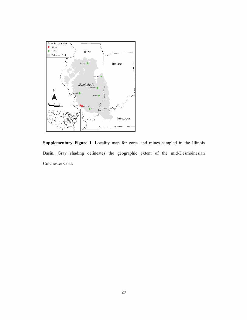
! 27!
Supplementary Figure 1. Locality map for cores and mines sampled in the Illinois
Basin. Gray shading delineates the geographic extent of the mid-Desmoinesian
Colchester Coal.
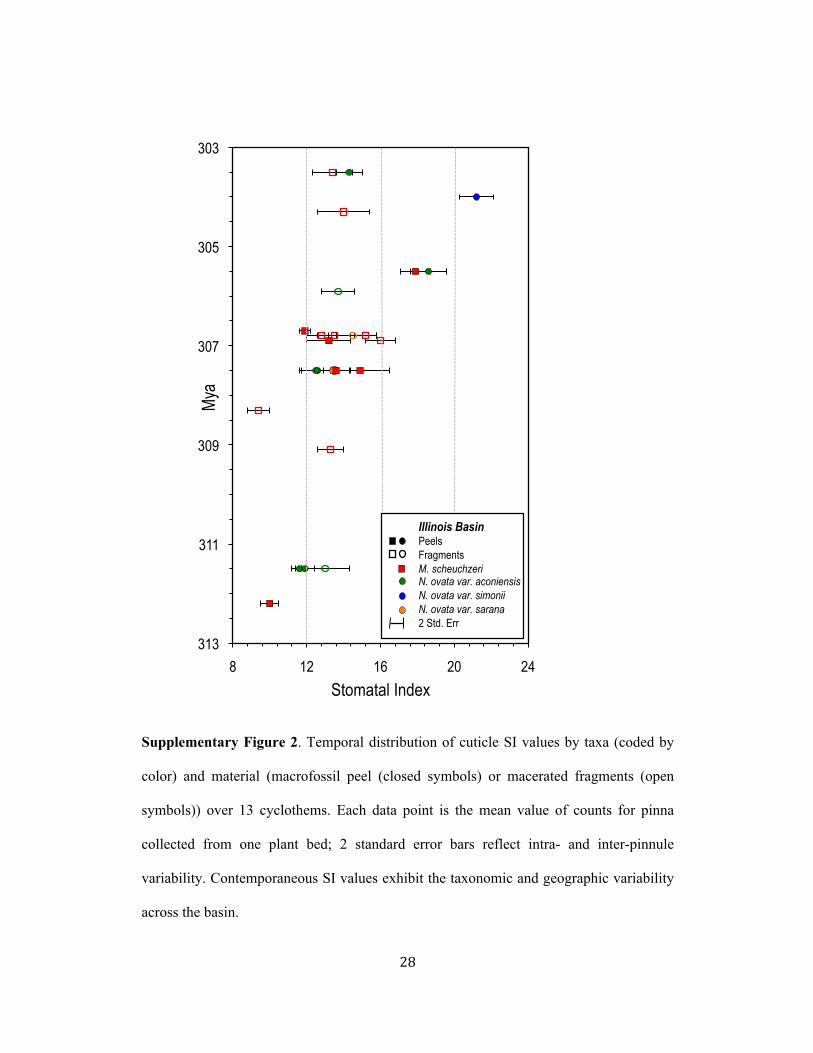
! 28!
Supplementary Figure 2. Temporal distribution of cuticle SI values by taxa (coded by
color) and material (macrofossil peel (closed symbols) or macerated fragments (open
symbols)) over 13 cyclothems. Each data point is the mean value of counts for pinna
collected from one plant bed; 2 standard error bars reflect intra- and inter-pinnule
variability. Contemporaneous SI values exhibit the taxonomic and geographic variability
across the basin.
303
305
307
309
311
313
8 12 16 20 24
Illinois Basin Peels Fragments M. scheuchzeri N. ovata var. aconiensis N. ovata var. simonii N. ovata var. sarana 2 Std. Err
Stomatal Index
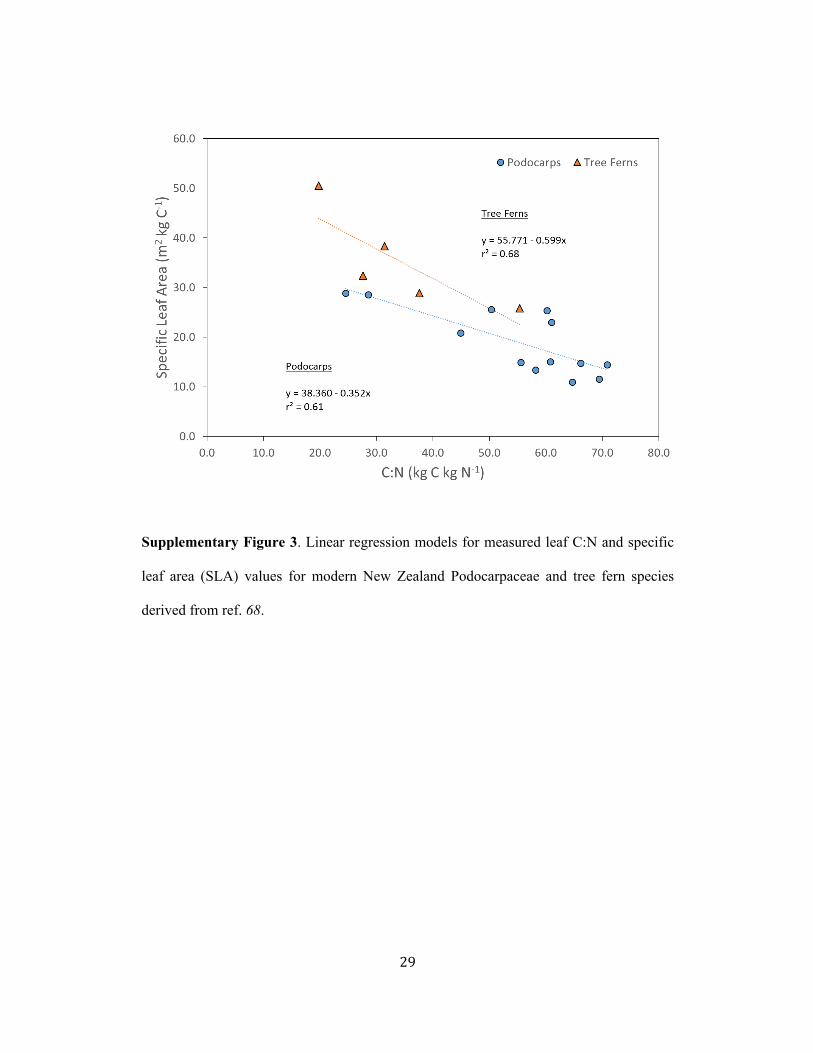
! 29!
Supplementary Figure 3. Linear regression models for measured leaf C:N and specific
leaf area (SLA) values for modern New Zealand Podocarpaceae and tree fern species
derived from ref. 68.

! 30!
Supplementary Figure 4. Comparison of modeled best estimates of pCO2, plotted by
paleosol type and presented as median (open symbols) and interquartile mean (filled
symbols) values. Trend lines are 3-pt running averages through the two sets of data.
0
100
200
300
400
500
600
700
800
900
296 298 300 302 304 306 308
Interquartile Mean Values: Vertisols Interquartile Mean Values: Argillisols & Protosols Interquartile Mean Values: Calcisols Median Values: Vertisols
Median Values: Argillisols & Protosols Median Values: Calcisols
Mod
eled
[CO
2] (
ppm
v)
Age (Myr)
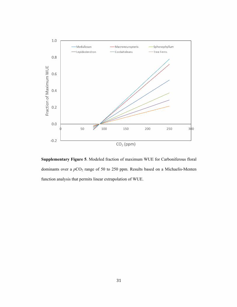
! 31!
Supplementary Figure 5. Modeled fraction of maximum WUE for Carboniferous floral
dominants over a pCO2 range of 50 to 250 ppm. Results based on a Michaelis-Menten
function analysis that permits linear extrapolation of WUE.
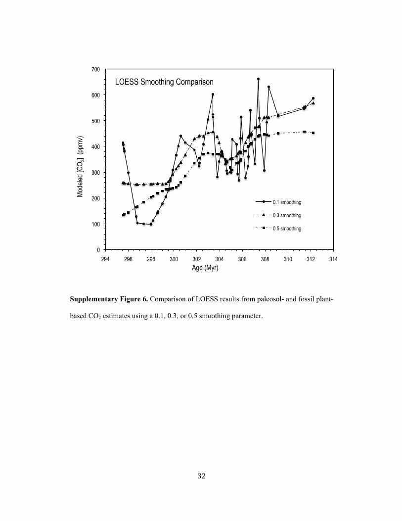
! 32!
Supplementary Figure 6. Comparison of LOESS results from paleosol- and fossil plant-
based CO2 estimates using a 0.1, 0.3, or 0.5 smoothing parameter.
0
100
200
300
400
500
600
700
294 296 298 300 302 304 306 308 310 312 314
0.1 smoothing
0.3 smoothing
0.5 smoothing
LOESS Smoothing Comparison M
odel
ed [C
O2]
(ppm
v)
Age (Myr)
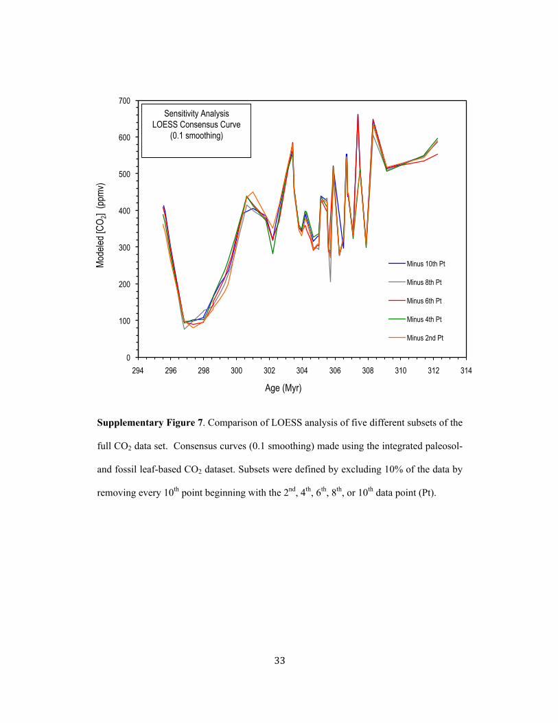
! 33!
Supplementary Figure 7. Comparison of LOESS analysis of five different subsets of the
full CO2 data set. Consensus curves (0.1 smoothing) made using the integrated paleosol-
and fossil leaf-based CO2 dataset. Subsets were defined by excluding 10% of the data by
removing every 10th point beginning with the 2nd, 4th, 6th, 8th, or 10th data point (Pt).
0
100
200
300
400
500
600
700
294 296 298 300 302 304 306 308 310 312 314
Minus 10th Pt
Minus 8th Pt
Minus 6th Pt
Minus 4th Pt
Minus 2nd Pt
Sensitivity Analysis LOESS Consensus Curve
(0.1 smoothing)
Age (Myr)
Mod
eled
[CO
2] (p
pmv)

! 34!
Supplementary Figure 8. Time series of (a) modeled Northern Hemisphere tropical
terrestrial MAP, (b) orbital regime used for climate simulation (560 ppm CO2), and (c)
ice volume, glacioeustatic response, and depositional model through one eccentricity
glacial-interglacial cycle. Ice sheet phase indicated as I: early glacial; II: peak glacial; III:
late glacial; IV: deglaciation and interglacial. Stippled region bounded by dashed lines
indicates the likely interval of transition from a dominantly erosive regime to peat
accumulation. This reflects the point at which the rate of sea-level fall is outpaced by the
regional subsidence rate, thus providing accommodation space for peat accumulation.
Modified from ref. 78.

Supplementary Table 1. A
ge model for the pC
O2 reconstruction and sam
ple distribution.
Age
1
(Mya)
MC
B2
Lithostratigraphic U
nits3
Midcontinent
Major C
yclothem4
Major C
oals (Illinois B
asin)M
idcontinent
Lithostrat. E
quiv. 5
Appalachian B
asin
Lithostrat. E
quiv. 6
Donets B
asin
Lithostrat. E
quiv. 7
Major
IVF
8Sam
ples (this study) 9
298 - >296G
reene Fm, D
unkard (AB
)D
UN
4-10; GR
E 2 & 3
298 - 299.5W
ashington Fm, D
unkard (AB
)1763:1-3; D
UN
1-3; WA
SH 1
299.30Q
4 paleosols (DB
)
KQ
11299.5 - 300.5
Waynesburg A
, Washington Fm
, Dunkard (A
B)
KV
180A299.50
P5-1 paleosols (DB
) P5-1
300.40P5 paleosols (D
B)
300.40
Monongahela G
p, Fishpot Lmst. (A
B)
18902: 1-3300.60
P4/5 paleosols (DB
)P4-P5
301.00upperm
ost Conem
augh Gp (A
B)
KV
182301.79
MC
BG
reenup Limestone
Topeka (H
olt)P2?
XELY
10302.19
MC
BSham
rock & N
ewton Lim
estones
Deer C
k (Larsh)P1
ELY 5; C
HA
1; CH
3302.60
MC
BB
ogota Limestone
Lecompton
Lecompton Lim
estonepossibly the G
aysportO
7? C
H 8; C
HA
2303.00
MC
BShum
way Lim
estone O
read
Oread Lim
estoneA
mes Lim
estoneO
6 C
H 9; C
HA
4303.40
Conem
augh Gp: Pittsburgh C
oal (AB
)Skelley
1712303.45
MC
BO
mega Lim
estoneC
assC
ass Limestone
O5
303.55H
arlem C
oal (AB
) H
arlemG
9HarlR
Hz 1-3; H
22 H
C-PR
B 1-4; P1-P6
303.70proposed K
asim-G
zhelian bdry (in Heebner Shale)
303.70M
issourian-Virgilian bdry (base of Cass cycle)
X303.76
Calhoun &
Shelbyville coals
fossil plants
303.80Little Verm
illion Limestone
Stanton Limestone
Noble/M
ill Ck lm
sts.O
4-6H
CH
13303.84
MC
BEudora Shale (M
C)
Stanton303.96
Cohn &
McC
leary's Bluff coals
ELY 30-32; fossil plants
304.13U
. Millersville-La Salle-
Livingston Limestone
limestone unit split into 3 parts:top
Iola Limestone
CH
A 8
304.16Friendsville C
oalbetw
een 2nd & 3rd part of lim
estone unitELY
36, 37
304.22L. M
illersville-La Salle- Livingston Lm
st.lim
estone unit split into 3 parts:bottomIola Lim
estoneC
H 16 &
21 304.25
MC
BM
uncie Creek Shale (M
C)
Iola
O4-3H
304.26
Bristol H
ill Coal
Portersville/Woods R
unELY
42 & 44; fossil plants
304.42C
offeen Limestone
304.45
Flannigan Coal
304.52R
eel Limestone
ELY 48

Supplementary Table 1. A
ge model for the pC
O2 reconstruction and sam
ple distribution.
Age
1
(Mya)
MC
B2
Lithostratigraphic U
nits3
Midcontinent
Major C
yclothem4
Major C
oals (Illinois B
asin)M
idcontinent
Lithostrat. E
quiv. 5
Appalachian B
asin
Lithostrat. E
quiv. 6
Donets B
asin
Lithostrat. E
quiv. 7
Major
IVF
8Sam
ples (this study) 9
304.62H
all Limestone
Dew
ey Limestone
LSC 17 &
21304.65
MC
BQ
uivira Shale (MC
)D
ewey
O
4-1 X
304.66Flat C
k Coal
C
ambridge/N
adine lmsts.
C
HA
10; CH
25304.82
Sorento Limestone
Cherryvale Fm
O3
304.88Fairbanks C
oal
305.02C
arthage Limestone
Upper B
rush Ck
LSC 11, 12, 14, 24, 64; C
H 29,
32; CH
A 11 &
14305.06
MC
BShoal C
kD
ennisD
ennis Lmst. (Stark Shale)
Pine Ck
O2
X305.07
New
Haven C
oal 305.43
Macoupin Lim
estoneSw
ope Limestone
Lower B
rush Ck
305.46M
CB
Hushpuckney Shale (M
C)
Swope
O
1
305.49W
omac coal (end hypothesized
strat. gap (Wagner &
Lyons 1997))W
omac
ELY 66 &
68; MA
C 10; V
ER 2-
4, 8, 9; CH
A 16; C
H 35; fossil
plants305.70
Carlinville Lim
estone N
5-2? M
AC
8305.73
Cram
er Limestone
Hertha Lim
estone305.76
MC
BM
ound City Shale (M
C)
Hertha
N5-1
305.79C
hapel coalC
hapel LSC
5; fossil plants
305.83Exline Lim
estone (prev. Scottsville); upper W
est Franklin Lm
st.Possible base of K
asimovian
Exline Limestone
N5
ELY 57A
305.86 M
AJOR FLO
RAL STEP CH
ANG
E
305.89A
thensville Coal
Athensville C
oal (#8)C
heckerboard S-Md
Mason C
oalfossil plants
306.00D
esmoinesian-M
issourian Bdry306.10
MC
BSem
inole SandstoneLost B
ranchX
X
306.23Lonsdale Lim
estone (midddle
West Franklin Lim
estone)Lost B
ranch Fm
N3-3 (306.08)
LSC 36
306.28A
tilla Shale
MA
C 26 &
28306.29
Rock B
ranch Coal
Daw
son Coal
Mahoning C
oalX
306.31M
CB
Gim
let Sandstone (&w
idespread paleosol)
Altam
ont(beginning of hypothesized stratigraphic gap (W
agner and Lyons, 1997))X
X
306.40D
e Graff C
oalpossibly equiv to Pirtle
306.50Piasa Lim
estone (lower W
est Franklin Lim
estone)
Altam
ont Limestone
N
3-1 C
HA
18-20; LSC 4, 36
306.60
Farmington Shale
Current correlated base of K
asimovian
Farlington ShaleN
3
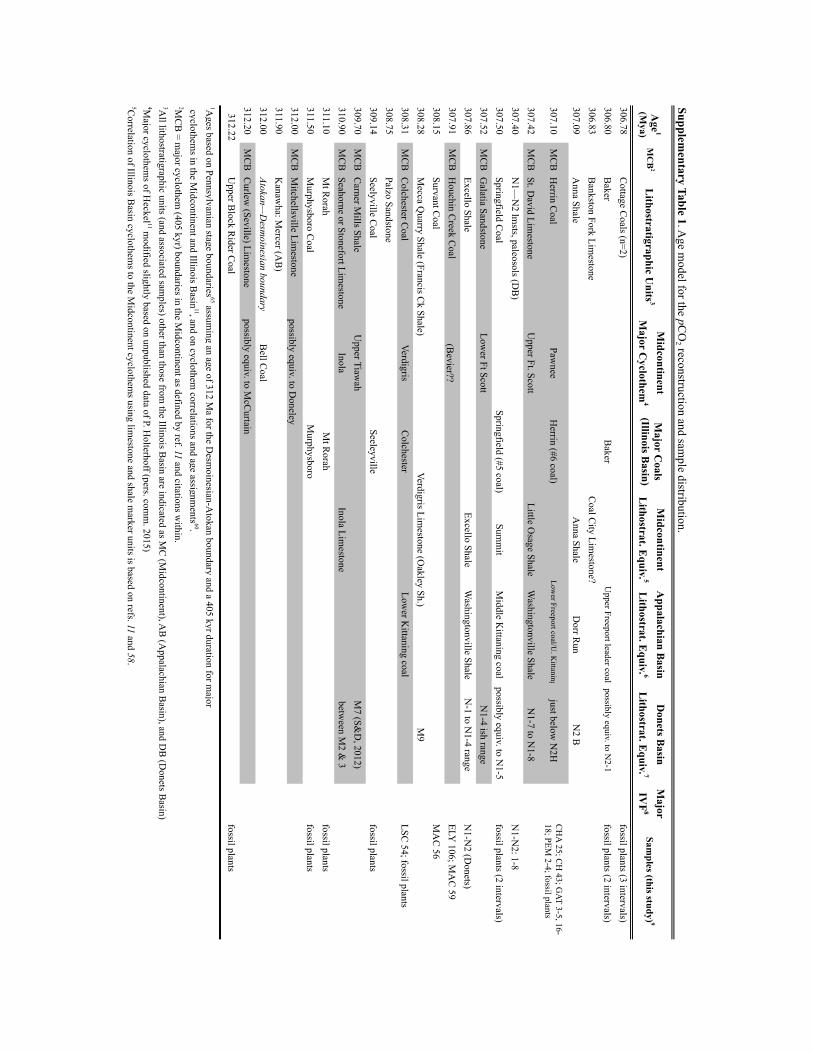
Supplementary Table 1. A
ge model for the pC
O2 reconstruction and sam
ple distribution.
Age
1
(Mya)
MC
B2
Lithostratigraphic U
nits3
Midcontinent
Major C
yclothem4
Major C
oals (Illinois B
asin)M
idcontinent
Lithostrat. E
quiv. 5
Appalachian B
asin
Lithostrat. E
quiv. 6
Donets B
asin
Lithostrat. E
quiv. 7
Major
IVF
8Sam
ples (this study) 9
306.78C
ottage Coals (n=2)
fossil plants (3 intervals)
306.80B
aker
Baker
Upper Freeport leader coal possibly equiv. to N
2-1fossil plants (2 intervals)
306.83B
ankston Fork Limestone
C
oal City Lim
estone?307.09
Anna Shale
Anna Shale
Dorr R
unN
2 B
307.10M
CB
Herrin C
oalPaw
neeH
errin (#6 coal)Low
er Freeport coal/U. K
ittaning just below
N2H
C
HA
25; CH
43; GAT 3-5, 16-
18; PEM 2-4; fossil plants
307.42M
CB
St. David Lim
estoneU
pper Ft. ScottLittle O
sage ShaleW
ashingtonville ShaleN
1-7 to N1-8
307.40N
1—N
2 lmsts, paleosols (D
B)
N1-N
2: 1-8307.50
Springfield Coal
Springfield (#5 coal)Sum
mit
Middle K
ittaning coalpossibly equiv. to N
1-5 fossil plants (2 intervals)
307.52M
CB
Galatia Sandstone
Lower Ft Scott
N1-4 ish range
307.86Excello Shale
Excello ShaleW
ashingtonville ShaleN
-1 to N1-4 range
N1-N
2 (Donets)
307.91M
CB
Houchin C
reek Coal
(Bevier??
ELY
106; MA
C 59
308.15
Survant Coal
M
AC
56308.28
Mecca Q
uarry Shale (Francis Ck Shale)
Verdigris Limestone (O
akley Sh.)M
9308.31
MC
BC
olchester Coal
VerdigrisC
olchester
Lower K
ittaning coalLSC
54; fossil plants308.75
Palzo Sandstone
309.14
Seelyville Coal
Seeleyville
fossil plants
309.70M
CB
Carner M
ills ShaleU
pper Tiawah
M7 (S&
D, 2012)
310.90M
CB
Seahorne or Stonefort Limestone
InolaInola Lim
estonebetw
een M2 &
3311.10
M
t Rorah
M
t Rorah
fossil plants
311.50
Murphysboro C
oal
Murphysboro
fossil plants312.00
MC
BM
itchellsville Limestone
possibly equiv. to Doneley
311.90
Kanaw
ha: Mercer (A
B)
312.00Atokan—
Desm
oinesian boundaryB
ell Coal
312.20M
CB
Curlew
(Seville) Limestone
possibly equiv. to McC
urtain
312.22U
pper Block R
ider Coal
fossil plants
1Ages based on Pennsylvanian stage boundaries
65 assuming an age of 312 M
a for the Desm
oinesian-Atokan boundary and a 405 kyr duration for m
ajor cyclothem
s in the Midcontinent and Illinois B
asin11, and on cyclothem
correlations and age assignments 60.
2MC
B = m
ajor cyclothem (405 kyr) boundaries in the M
idcontinent as defined by ref. 11 and citations within.
3All lithostratigraphic units (and associated sam
ples) other than those from the Illinois B
asin are indicated as MC
(Midcontinent), A
B (A
ppalachian Basin), and D
B (D
onets Basin)
4Major cyclothem
s of Heckel 11 m
odified slightly based on unpublished data of P. Holterhoff (pers. com
m. 2015)
5Correlation of Illinois B
asin cyclothems to the M
idcontinent cyclothems using lim
estone and shale marker units is based on refs. 11 and 58.

6Correlation of Illinois B
asin cyclothems to the A
ppalachian Basin cyclothem
s using limestones and coals is based on ref. 11 and citations w
ithin.7C
orrelation of Illinois Basin cyclothem
s to the Donets B
asin cyclothems after refs. 58-60.
8Stratigraphic distribution of major incised valley fills (IV
F) as defined by refs. 11, 19, and 58. Double X
indicates deepest incision channels in succession (>30 to 40+ m
) 19. Note: IV
F underlie limestone units for w
hich Midcontinent cyclothem
s are named.
9Core location (see Supplem
entary Fig. 1) of samples indicated by: Lonestar (LSC
), Vermillion (V
ER), C
harleston (CH
& C
HA
), Elysium (ELY
), Macoupin (M
AC
), Gatew
ay (GAT), D
emier (D
EM)

Supplementary Table 2. Input variables for PB
UQ
and modeled C
O2 based on pedogenic carbonates
1Age
Sample (n)
2Stratigraphic Marker B
ed or Unit
Soil Order/type
(Mya)
‰
(± 1σ)
‰
(± 1σ)
*300.2H
T 1-3, (7)H
onaker Trail Fm, U
Tsandy C
alcisols-3.4
0.6-20.5
1.0
*299.9N
1: 1-2, (2)H
ermit Shale Fm
, Kohl’s R
anch, AZ
Calcisols
-4.21.1
-20.51.0
*299.7B
F 1-7, (5)B
ursum Fm
, Socorro, NM
Calcisols
-6.10.3
-21.01.1
*299.5H
AL 1-4, 7, 9, 12, 17, 18, 22,
25-26, 48, (16)upper H
algaito Fm, A
Zsilty C
alcisols-4.0
0.2-20.5
0.8
*298.6S4, (3)
Herm
it Shale Fm, Flagstaff, A
Z (upper set)m
uddy Calcisols
-5.40.2
-20.50.8
*298.5S2, (2)
Herm
it Shale Fm, Flagstaff, A
Z (lower set)
muddy C
alcisols-6.7
0.1-20.5
0.8
*298.2A
C 31-32, (2)
middle A
rcher City Fm
, stratotype (SS5), nc-TXcalcic Vertisols
-7.11.5
-21.30.5
*298.0A
BB
A 3-9; A
CB
BH
/R, (4)
upper Archer C
ity Fm bonebed (SS8), nc-TX
Alfisols
-9.41.0
-21.30.5
*297.4N
BC
2 & 4, (3)
basal Nocona Fm
, coprolite bonebed, nc-TXcalcic Vertisols
-9.51.0
-21.31.1
*296.8N
LAD
2 & 99
middle N
ocona Fm, nc-TX
calcic Vertisols-8.6
0.8-21.3
1.1
*296.7A
3-10, (11)A
bo Fm, Socorro to Las C
ruces, NM
calcic Vertisols-5.6
0.6-21.4
0.7
296.0D
unkard 4-10, (12)G
reene Fm, D
unkard Gp. A
ppal. Basin
calcic Vertisols-8.9
1.2-24.5
1.0
296.0G
RE 2 &
3, (4)G
reene Fm, D
unkard Gp. A
ppal. Basin
calcic Vertisols-8.0
0.3-24.5
1.0
298.0D
UN
1-3, (6)W
ashington Fm, D
unkard Gp. A
ppal. Basin
calcic Vertisols-9.0
0.5-24.1
0.4
299.0W
ASH
1, (2)W
ashington Fm, D
unkard Gp. A
ppal. Basin
calcic Vertisols-11.7
0.0-24.1
0.4
299.3K
Q 11, (8)
Q4 Lim
estone, Donets B
asinA
rgillisol-6.4
0.1-23.8
0.3
Pedogenic
δ13C
carb
3Respired C
O2
δ13C
: discrete org
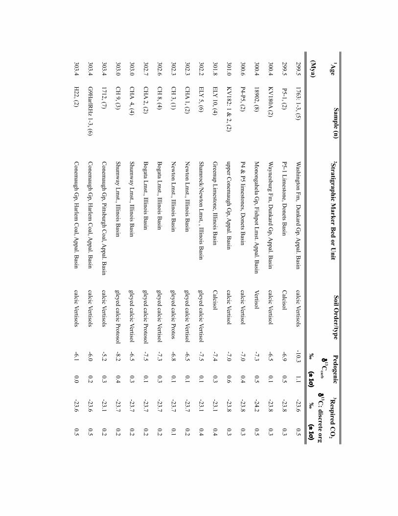
1Age
Sample (n)
2Stratigraphic Marker B
ed or Unit
Soil Order/type
(Mya)
‰
(± 1σ)
‰
(± 1σ)
299.51763: 1-3, (5)
Washington Fm
, Dunkard G
p. Appal. B
asincalcic Vertisols
-10.31.1
-23.60.5
299.5 P5-1, (2)
P5-1 Limestone, D
onets Basin
Calcisol
-6.90.5
-23.80.3
300.4K
V180A
(2)W
aynesburg Fm, D
unkard Gp, A
ppal. Basin
calcic Vertisol-6.5
0.1-23.8
0.3
300.418902, (8)
Monongahela G
p, Fishpot Lmst. A
ppal. Basin
Vertisol-7.3
0.5-24.2
0.5
300.6P4-P5, (2)
P4 & P5 lim
estones, Donets B
asincalcic Vertisol
-7.00.4
-23.80.3
301.0K
V182: 1 &
2, (2)upper C
onemaugh G
p, Appal. B
asincalcic Vertisol
-7.00.6
-23.80.3
301.8ELY
10, (4)G
reenup Limestone, Illinois B
asinC
alcisol-7.4
0.3-23.1
0.4
302.2ELY
5, (6)Sham
rock/New
ton Lmst, , Illinois B
asingleyed calcic Vertisol
-7.50.1
-23.10.4
302.3C
HA
1, (2)N
ewton Lm
st., Illinois Basin
gleyed calcic Vertisol-6.5
0.1-23.7
0.2
302.3C
H 3, (1)
New
ton Lmst., Illinois B
asingleyed calcic Protos
-6.80.1
-23.70.1
302.6C
H 8, (4)
Bogata Lm
st., Illinois Basin
gleyed calcic Vertisol-7.3
0.3-23.7
0.2
302.7C
HA
2, (2)B
ogata Lmst., Illinois B
asingleyed calcic Protosol
-7.50.1
-23.70.2
303.0C
HA
4, (4)Shum
way Lm
st., Illinois Basin
gleyed calcic Vertisol-6.5
0.3-23.7
0.2
303.0C
H 9, (3)
Shumw
ay Lmst., Illinois B
asingleyed calcic Protosol
-8.20.4
-23.70.2
303.41712, (7)
Conem
augh Gp, Pittsburgh C
oal, Appal. B
asincalcic Vertisols
-5.20.3
-23.10.2
303.4G
9HarlR
Hz 1-3, (6)
Conem
augh Gp, H
arlem C
oal, Appal. B
asincalcic Vertisols
-6.00.2
-23.60.5
303.4H
22, (2)C
onemaugh G
p, Harlem
Coal, A
ppal. Basin
calcic Vertisols-6.1
0.0-23.6
0.5
Pedogenic
δ13C
carb
3Respired C
O2
δ13C
: discrete org

1Age
Sample (n)
2Stratigraphic Marker B
ed or Unit
Soil Order/type
(Mya)
‰
(± 1σ)
‰
(± 1σ)
303.4H
C-PR
B-1-4, (12)
Conem
augh Gp, H
arlem C
oal, Appal. B
asincalcic Vertisols
-6.70.5
-23.60.5
303.4P1-1-5, (8)
Conem
augh Gp, H
arlem C
oal, Appal. B
asincalcic Vertisol
-6.00.2
-23.60.5
303.4P5-1-4, (5)
Conem
augh Gp, H
arlem C
oal, Appal. B
asincalcic Vertisol
-5.51.0
-23.60.5
303.4P3-1-5, (11)
Conem
augh Gp, H
arlem C
oal, Appal. B
asincalcic Vertisol
-5.60.8
-23.60.5
303.4P6-1-5, (8)
Conem
augh Gp, H
arlem C
oal, Appal. B
asincalcic Vertisol
-6.90.2
-23.60.5
303.8C
H 13, (2)
Little Vermillion Lm
st., Illinois Basin
gleyed calcic Vertisol-8.7
0.1-24.5
0.5
304.0ELY
30-32, (5)C
ohn Coal, Illinois B
asingleyed calcic Vertisol
-8.10.3
-24.50.5
304.1C
HA
8, (3)M
illersville Lmst., Illinois B
asincalcic Protosol
-8.10.2
-24.10.3
304.2ELY
36 & 37, (4)
Friendsville Coal, Illinois B
asingleyed calcic Vertisol
-7.70.9
-24.50.5
304.2C
H 16, (4)
Lower M
illersville Lmst., Illinois B
asingleyed calcic Vertisol
-8.30.2
-24.10.3
304.2C
H 21, (3)
Lower M
illersville Lmst., Illinois B
asingleyed calcic Protosol
-8.10.4
-24.10.3
304.3ELY
44 & 42, (4)
Bristol C
oal, Illinois Basin
gleyed calcic Vertisol-8.0
0.6-24.5
0.5
304.5ELY
48, (2)R
eel Lmst., Illinois B
asingleyed C
alcisol-8.9
0.0-25.3
0.7
304.6LSC
17 & 21, (6)
Lower H
all Lmst, Illinois B
asincalcic Vertisol
-8.40.3
-25.01.0
304.7C
H 25 &
CH
A 10, (6)
Flat Creek C
oal, Illinois Basin
gleyed calcic Vertisol-8.2
0.5-24.6
1.1
304.9C
H 29, (4)
above Carthage Lm
st, Illinois Basin
gleyed Calcisol
-8.30.1
-24.01.2
305.0LSC
11-12, 14, (6)C
arthage Lmst., Illinois B
asinVertisol
-8.20.3
-24.01.0
Pedogenic
δ13C
carb
3Respired C
O2
δ13C
: discrete org
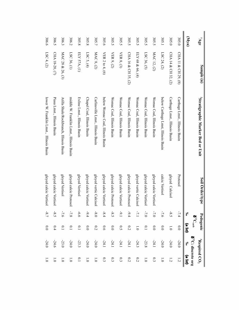
1Age
Sample (n)
2Stratigraphic Marker B
ed or Unit
Soil Order/type
(Mya)
‰
(± 1σ)
‰
(± 1σ)
305.0C
HA
11 & C
H 29, (8)
Carthage Lm
st., Illinois Basin
Protosol-7.4
0.0-24.0
1.2
305.0C
HA
14 & C
H 32, (2)
Carthage Lm
st., Illinois Basin
gleyed Calcisol
-8.51.0
-24.01.2
305.1LSC
24, (2)below
Carthage Lm
st, Illinois Basin
calcic Vertisol-7.6
0.0-24.0
1.0
305.5M
AC
12, (2)W
omac C
oal, Illinois Basin
gleyed calcic Vertisol-7.0
0.0-24.1
0.3
305.5LSC
36, (5)W
omac C
oal, Illinois Basin
gleyed calcic Vertisol-7.0
0.1-23.8
1.0
305.5ELY
68 & 66, (4)
Wom
ac Coal, Illinois B
asingleyed vertic C
alcisol-7.1
1.0-24.3
0.2
305.5C
HA
16 & C
H 35, (2)
Wom
ac Coal, Illinois B
asingleyed calcic Protosol
-9.40.2
-24.10.2
305.5V
ER 8, (3)
Wom
ac Coal, Illinois B
asingleyed calcic Vertisol
-9.10.5
-24.10.3
305.5V
ER 9, (2)
Wom
ac Coal, Illinois B
asingleyed calcic Protosol
-8.50.0
-24.10.3
305.6V
ER 2 to 4, (6)
below W
omac C
oal, Illinois Basin
gleyed calcic Vertisol-8.4
0.6-24.1
0.3
305.7M
AC
8, (2)C
arlinsville Lmst., Illinois B
asingleyed vertic C
alcisol-8.0
0.2-24.0
1.0
305.8LSC
5, (4)C
hapel Coal, Illinois B
asingleyed calcic Vertisol
-9.40.0
-24.01.0
305.8ELY
57A, (1)
Exline Lmst., Illinois B
asingleyed Vertisol
-6.60.1
-23.30.1
306.2LSC
36, (1)m
iddle W. Franklin Lm
st., Illinois Basin
gleyed calcic Protosol-7.8
0.1-24.0
1.0
306.3M
AC
28 & 26, (3)
Atilla Shale/R
ockbranch, Illinois Basin
gleyed Vertisol-7.6
0.1-23.0
1.0
306.5C
HA
18-20, (7)Piasa Lm
st., Illinois Basin
gleyed calcic Vertisol-8.5
0.4-24.6
1.0
306.6LSC
4, (2)low
er W. Franklin Lm
st., Illinois Basin
gleyed calcic Vertisol-8.7
0.0-24.0
1.0
Pedogenic
δ13C
carb
3Respired C
O2
δ13C
: discrete org
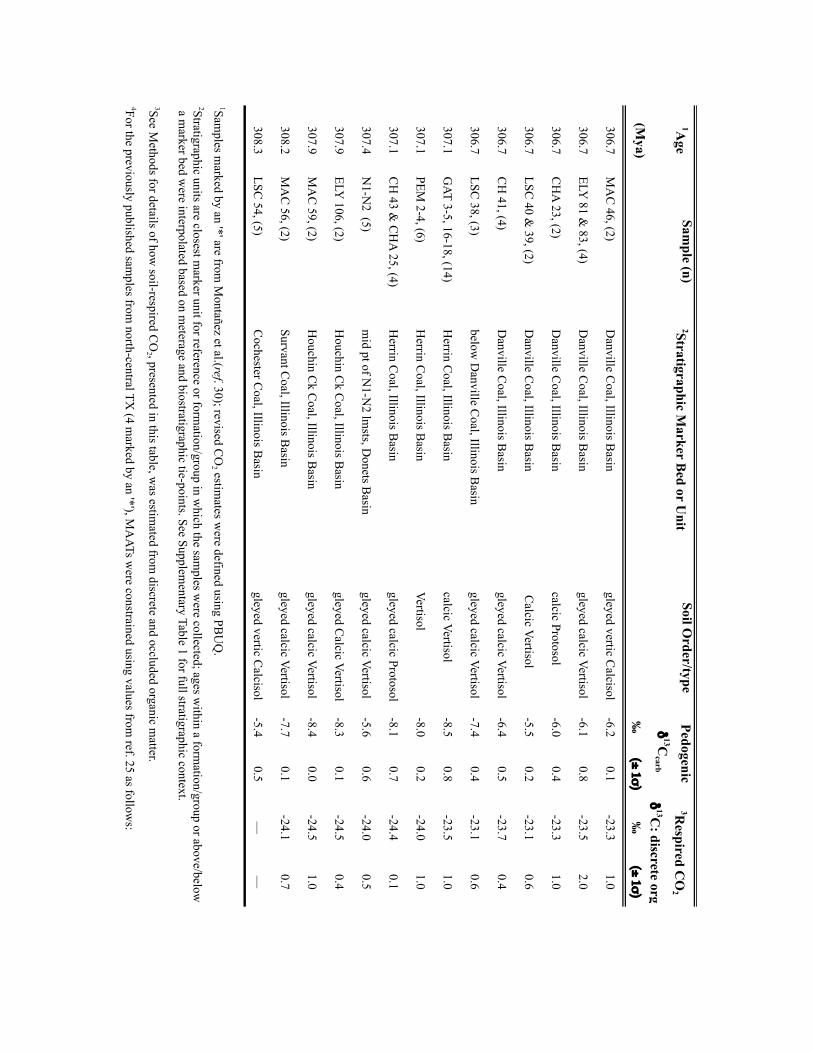
1Age
Sample (n)
2Stratigraphic Marker B
ed or Unit
Soil Order/type
(Mya)
‰
(± 1σ)
‰
(± 1σ)
306.7M
AC
46, (2)D
anville Coal, Illinois B
asingleyed vertic C
alcisol-6.2
0.1-23.3
1.0
306.7ELY
81 & 83, (4)
Danville C
oal, Illinois Basin
gleyed calcic Vertisol-6.1
0.8-23.5
2.0
306.7C
HA
23, (2)D
anville Coal, Illinois B
asincalcic Protosol
-6.00.4
-23.31.0
306.7LSC
40 & 39, (2)
Danville C
oal, Illinois Basin
Calcic Vertisol
-5.50.2
-23.10.6
306.7C
H 41, (4)
Danville C
oal, Illinois Basin
gleyed calcic Vertisol-6.4
0.5-23.7
0.4
306.7LSC
38, (3)below
Danville C
oal, Illinois Basin
gleyed calcic Vertisol-7.4
0.4-23.1
0.6
307.1G
AT 3-5, 16-18, (14)H
errin Coal, Illinois B
asincalcic Vertisol
-8.50.8
-23.51.0
307.1PEM
2-4, (6)H
errin Coal, Illinois B
asinVertisol
-8.00.2
-24.01.0
307.1C
H 43 &
CH
A 25, (4)
Herrin C
oal, Illinois Basin
gleyed calcic Protosol-8.1
0.7-24.4
0.1
307.4N
1-N2 (5)
mid pt of N
1-N2 lm
sts, Donets B
asingleyed calcic Vertisol
-5.60.6
-24.00.5
307.9ELY
106, (2)H
ouchin Ck C
oal, Illinois Basin
gleyed Calcic Vertisol
-8.30.1
-24.50.4
307.9M
AC
59, (2)H
ouchin Ck C
oal, Illinois Basin
gleyed calcic Vertisol-8.4
0.0-24.5
1.0
308.2M
AC
56, (2)Survant C
oal, Illinois Basin
gleyed calcic Vertisol-7.7
0.1-24.1
0.7
308.3LSC
54, (5)C
ochester Coal, Illinois B
asingleyed vertic C
alcisol-5.4
0.5—
—
1Samples m
arked by an '*' are from M
ontañez et al.(ref. 30); revised CO
2 estimates w
ere defined using PBU
Q.
2Stratigraphic units are closest marker unit for reference or form
ation/group in which the sam
ples were collected; ages w
ithin a formation/group or above/below
a m
arker bed were interpolated based on m
eterage and biostratigraphic tie-points. See Supplementary Table 1 for full stratigraphic context.
3See Methods for details of how
soil-respired CO
2 , presented in this table, was estim
ated from discrete and occluded organic m
atter.4For the previously published sam
ples from north-central TX
(4 marked by an '*'), M
AATs w
ere constrained using values from ref. 25 as follow
s:
Pedogenic
δ13C
carb
3Respired C
O2
δ13C
: discrete org

(1) for proxy soil temperatures > 30°C
, then MA
AT 5°C low
er, (2) for proxy soil temperatures >25°C
to ≤ 30°C, then M
AAT 3°C
lower, and (3) for proxy soil
temperatures ≤ 25°C
, then MA
AT = soil temperature. M
AATs for sam
ples from A
Z, NM
, and UT w
ere similarly assigned based on stratigraphic equivalent
intervals from TX
.5B
est estimate of pC
O2 based on trim
med m
ean. For those samples for w
hich the δ13C
of the organic matter occluded in pedogenic carbonates w
as analyzed, the best estim
ate pCO
2 utilized those input values.6A
n alternative pCO
2 estimate, based on the δ
13C of discrete organic m
atter closely associated with the paleosol, is provided for those sam
ples for which
soil-respired CO
2 was constrained by both discrete and occluded organic m
atter.

Supplementary Table 2.
4Temp.
°C
5Best E
stimate
CO
216%
84%6A
lt. Estim
ate CO
2
(16/84 %)
‰
(± 1σ)
(± 3°)‰
(± 1σ
)ppm
ppmppm
ppm
——
24.04.6
0.2331
128695
——
24.04.6
0.2247
76548
——
24.04.7
0.2128
37287
——
24.04.7
0.2290
117590
—
——
26.04.8
0.2169
66350
—
——
26.04.8
0.283
21186
—
——
26.04.8
0.2158
10519
—
——
30.04.9
0.210
149
—
——
29.04.9
0.214
178
—
——
28.04.4
0.247
1183
—
——
28.04.4
0.2404
1011162
—
——
23.03.9
0.5242
46734
—
——
23.03.9
0.5349
85996
—
——
23.04.2
0.5194
47558
—
——
23.04.2
0.54
119
—
——
23.02.8
0.7380
270527
—
3Respired C
O2
δ13C
: occlud. org
Marine δ
13Ccarb

4Temp.
°C
5Best E
stimate
CO
216%
84%6A
lt. Estim
ate CO
2
(16/84 %)
‰
(± 1σ)
(± 3°)‰
(± 1σ
)ppm
ppmppm
ppm
-24.30.2
23.02.8
0.7193
42569
69 (1/265)
——
23.02.8
0.7258
106528
—
——
23.02.8
0.7550
1391573
—
-25.40.2
23.03.9
0.3675
1681902
450 (111/1291)
——
23.02.8
0.7461
1161318
—
——
23.03.0
0.5468
1161339
—
——
23.03.8
0.3199
57406
—
——
23.03.9
0.3284
72817
—
——
23.03.9
0.3483
1171389
—
——
23.03.9
0.3129
85184
—
——
23.04.0
0.4363
921033
—
——
23.04.0
0.498
63141
—
——
23.04.0
0.4505
1221449
—
——
23.04.0
0.474
45110
—
-23.00.2
23.03.9
0.4769
1922195
645 (162/1846)
——
23.03.9
0.4558
1381607
—
——
23.03.9
0.4528
1321508
—
3Respired C
O2
δ13C
: occlud. org
Marine δ
13Ccarb

4Temp.
°C
5Best E
stimate
CO
216%
84%6A
lt. Estim
ate CO
2
(16/84 %)
‰
(± 1σ)
(± 3°)‰
(± 1σ
)ppm
ppmppm
ppm
——
23.03.9
0.4440
1121260
—
——
23.03.9
0.4550
1391593
—
——
23.03.9
0.4607
1142305
—
-25.10.2
23.03.9
0.4905
2282535
609 (153/1732)
-25.10.2
23.03.9
0.4684
1651960
415 (103/1182)
——
23.03.9
0.4279
70800
—
——
23.03.9
0.4358
82990
—
-24.00.2
23.03.8
0.4114
72165
90 (58/131)
——
23.03.8
0.4398
981131
—
——
23.03.6
0.4289
73827
—
——
23.03.6
0.492
57134
—
——
23.03.6
0.4360
891048
—
——
23.03.5
0.5178
75364
—
-23.30.2
23.03.5
0.5303
76868
351 (89/1017)
-23.50.2
23.03.5
0.5395
84971
349 (83/1021)
——
23.03.4
0.5150
52319
—
——
23.03.4
0.5281
67807
—
3Respired C
O2
δ13C
: occlud. org
Marine δ
13Ccarb

4Temp.
°C
5Best E
stimate
CO
216%
84%6A
lt. Estim
ate CO
2
(16/84 %)
‰
(± 1σ)
(± 3°)‰
(± 1σ
)ppm
ppmppm
ppm
——
23.03.4
0.5112
62175
—
——
23.03.4
0.5139
36314
—
——
23.03.3
0.5436
1081230
—
——
23.03.2
0.5476
1191356
—
——
23.03.1
0.5454
1091293
—
——
23.03.1
0.5275
107569
—
——
23.03.1
0.552
3179
—
——
23.03.1
0.5212
52623
—
——
23.03.1
0.5108
69156
—
——
23.03.1
0.5288
71833
—
——
23.03.1
0.5171
67356
—
-22.90.2
23.03.1
0.5162
38477
158 (32/462)
——
23.03.1
0.5464
1161324
—
——
23.03.1
0.5102
57159
—
——
23.03.1
0.5274
63788
—
——
23.03.1
0.5315
77904
—
-23.90.2
23.03.1
0.5336
83968
241 (56/695)
3Respired C
O2
δ13C
: occlud. org
Marine δ
13Ccarb

4Temp.
°C
5Best E
stimate
CO
216%
84%6A
lt. Estim
ate CO
2
(16/84 %)
‰
(± 1σ)
(± 3°)‰
(± 1σ
)ppm
ppmppm
ppm
——
23.03.1
0.5282
115574
—
——
23.03.1
0.5519
381622
—
-23.60.2
23.03.1
0.5209
132307
162 (85/247)
——
23.03.1
0.5643
1601836
—
——
23.03.1
0.5549
1381591
—
-24.30.2
23.03.1
0.5640
1371583
322 (79/928)
-23.70.2
23.03.2
0.5325
80938
251 (39/612)
-22.90.2
23.03.2
0.5321
81916
319 (80/924)
——
23.03.2
0.5104
60159
—
——
23.04.0
0.6662
1671886
—
——
23.04.0
0.6314
79893
—
——
23.04.0
0.6299
73849
—
——
23.04.1
0.6338
88951
—
-23.80.2
23.04.1
0.6644
1571213
—
2Stratigraphic units are closest marker unit for reference or form
ation/group in which the sam
ples were collected; ages w
ithin a formation/group or above/below
3Respired C
O2
δ13C
: occlud. org
Marine δ
13Ccarb
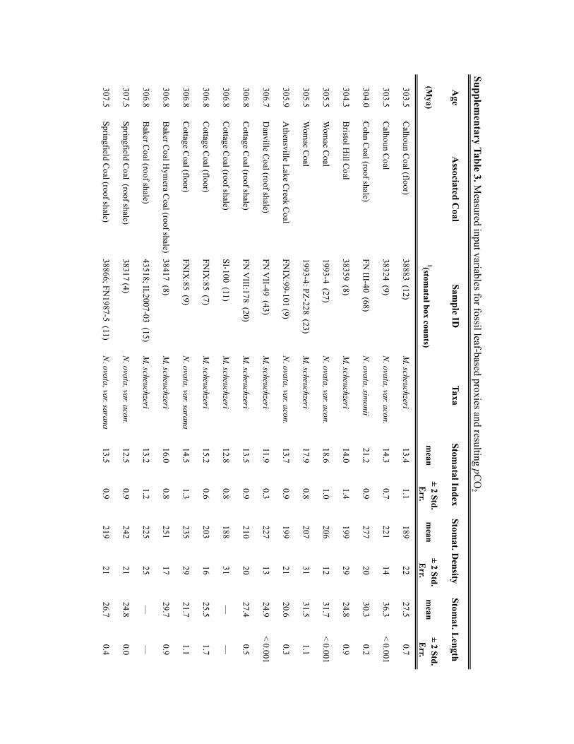
Supplementary Table 3. M
easured input variables for fossil leaf-based proxies and resulting pCO
2
Age
Associated C
oalSam
ple ID
Taxa
(Mya)
1(stomatal box counts)
mean
± 2 Std. E
rr.m
ean ± 2 Std.
Err.
mean
± 2 Std. E
rr.
303.5C
alhoun Coal (floor)
38883 (12)M
. scheuchzeri13.4
1.1189
2227.5
0.7
303.5C
alhoun Coal
38324 (9)N
. ovata, var. acon.14.3
0.7221
1436.3
< 0.001
304.0C
ohn Coal (roof shale)
FN III-40 (68)
N. ovata, sim
onii21.2
0.9277
2030.3
0.2
304.3B
ristol Hill C
oal38359 (8)
M. scheuchzeri
14.01.4
19929
24.80.9
305.5W
omac C
oal1993-4 (27)
N. ovata, var. acon.
18.61.0
20612
31.7< 0.001
305.5W
omac C
oal1993-4: PZ-228 (23)
M. scheuchzeri
17.90.8
20731
31.51.1
305.9A
thensville Lake Creek C
oal FN
IX:99-101 (9)
N. ovata, var. acon.
13.70.9
19921
20.60.3
306.7D
anville Coal (roof shale)
FN V
II-49 (43)M
. scheuchzeri11.9
0.3227
1324.9
< 0.001
306.8C
ottage Coal (roof shale)
FN V
III:178 (20)M
. scheuchzeri13.5
0.9210
2027.4
0.5
306.8C
ottage Coal (roof shale)
SI-100 (11)M
. scheuchzeri12.8
0.8188
31—
—
306.8C
ottage Coal (floor)
FNIX
:85 (7)M
. scheuchzeri15.2
0.6203
1625.5
1.7
306.8C
ottage Coal (floor)
FNIX
:85 (9)N
. ovata, var. sarana14.5
1.3235
2921.7
1.1
306.8B
aker Coal H
ymera C
oal (roof shale)38417 (8)
M. scheuchzeri
16.00.8
25117
29.70.9
306.8B
aker Coal (roof shale)
43518; IL2007-03 (15)M
. scheuchzeri13.2
1.2225
25—
—
307.5Springfield C
oal (roof shale)38317 (4)
N. ovata, var. acon.
12.50.9
24221
24.80.0
307.5Springfield C
oal (roof shale)38866; FN
1987-5 (11)N
. ovata, var. sarana13.5
0.9219
2126.7
0.4
Stomatal Index
Stomat. D
ensityStom
at. Length

Age
Associated C
oalSam
ple ID
Taxa
(Mya)
1(stomatal box counts)
mean
± 2 Std. E
rr.m
ean ± 2 Std.
Err.
mean
± 2 Std. E
rr.
307.5Springfield C
oal (roof shale)43499; FN
III-118 (8)N
. ovata, var. acon.12.6
0.9226
1127.3
0.0
307.5Springfield C
oal (roof shale)FN
VII-82 (12)
M. scheuchzeri
13.60.7
29923
27.00.0
307.5Springfield C
oal (roof shale)FN
VII-98 (5)
M. scheuchzeri
14.91.6
19239
——
308.3C
olchester Coal (roof shale)
38355 (4)M
. scheuchzeri9.4
0.6181
2719.0
1.1
309.1Seeleyville C
oal (roof shale)38314 (15)
M. scheuchzeri
13.30.7
23211
23.00.3
311.4M
urphysboro Coal: FN
II-111FN
II-111 (35)N
. ovata, var. acon.11.6
0.4184
1222.4
0.4
311.5M
urphysboro(floor)FN
8-114 (55)N
. ovata, var. acon.11.9
0.5223
1028.1
0.3
311.5M
urphysboro (floor)FN
II-111-112 (4)N
. ovata, var. acon.13.0
1.3193
2128.7
0.0
312.2U
pper Block R
iderFN
VII: 65-66 (7)
M. scheuchzeri
10.00.5
1104
30.60.0
1For each count, stomata w
ere measured w
ithin a square to rectangular box with a total area of 0.04 m
m2.
2Stomatal Index values w
ere calibrated to paleo-pCO
2 using the method of M
cElwain and C
haloner (ref. 49) and three nearest-living equivalents (NLE). The
stomatal ratio m
ethod13 applied an average SI of the three N
LEs of 18.1 and a Recent calibration. See M
ethods for more detail.
Stomatal Index
Stomat. D
ensityStom
at. Length

mean
± 2 Std. E
rr.‰
(± 1σ)
‰
rangem
ean ± 2 Std.
Err.
mean
16%84%
13.51.1
-24.80.3
-5.8-0.4/+0.2
49541
462322
701
20.2< 0.001
-24.80.3
-5.8-0.4/+0.2
45817
421293
649
13.30.4
-24.80.3
-5.8-1.3/+0.6
32221
393274
610
12.00.7
-25.10.3
-6.3±1.1
47552
472331
712
15.6< 0.001
-26.20.3
-6.5-1.1/+1.4
35419
507355
767
17.20.8
-26.20.3
-6.5-1.1/+1.5
36817
446260
690
9.50.3
-26.20.3
-6.5-1.2/+1.4
47726
582412
864
13.34.8
-25.50.3
-5.8-1.6/+1.1
55111
477332
730
14.40.4
-24.40.3
-5.8-0.4/+1.4
49234
480333
737
——
——
——
47350
——
—
13.30.8
-24.40.3
-5.8-0.4/+1.4
42940
431307
667
9.00.7
-24.40.3
-5.8-0.4/+1.4
45846
397277
610
15.40.5
-24.50.3
-5.8-0.4/+1.4
40922
358247
561
——
——
——
50950
——
—
13.20.0
-25.20.3
-5.6-0.4/+1.4
52235
536376
805
12.20.9
-25.20.3
-5.6-0.4/+1.4
48530
527371
795
Atm
. δ13C
carb M
echanistic pCO
2 2SI-based pC
O2
Stomatal W
idthC
uticle δ13C
org
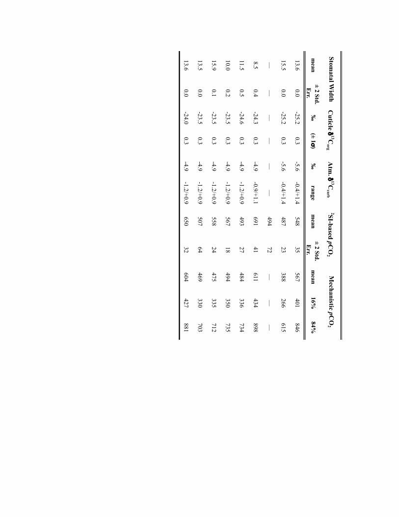
mean
± 2 Std. E
rr.‰
(± 1σ)
‰
rangem
ean ± 2 Std.
Err.
mean
16%84%
13.60.0
-25.20.3
-5.6-0.4/+1.4
54835
567401
846
15.50.0
-25.20.3
-5.6-0.4/+1.4
48723
388266
615
——
——
——
49472
——
—
8.50.4
-24.30.3
-4.9-0.9/+1.1
69141
611434
898
11.50.5
-24.60.3
-4.9-1.2/+0.9
49327
484336
734
10.00.2
-23.50.3
-4.9-1.2/+0.9
56718
494350
735
15.90.1
-23.50.3
-4.9-1.2/+0.9
55824
475335
712
13.50.0
-23.50.3
-4.9-1.2/+0.9
50764
469330
703
13.60.0
-24.00.3
-4.9-1.2/+0.9
65032
604427
881
Atm
. δ13C
carb 2SI-based pC
O2
Mechanistic pC
O2
Stomatal W
idthC
uticle δ13C
org

! 35!
Supplementary Table 4. Parameter descriptors, data input ranges and scaling factors
used to estimate pCO2 from fossil Neuropteris ovata and Macroneuropteris scheuchzeri
Input Description Range of input values Reference/Justification/Method
#Dab: stomatal density (m2) on abaxial surface
99.34 to 375 mm2 Measured on fossil cuticles
#eDab error in Dab in m2 9.93 to 37.5 mm2 1σ uncertainty of fossil cuticle measurements
#Dad: stomatal density (m2)
0 All fossil species hypostomatous
#eDad: error in Dad 0 All fossil species hypostomatous
#GCLab: guard cell length (m) on abaxial surface
17.84 to 37.73 µm Measured directly from cuticles. Where guard cell length could not be directly measured because stomata were sunken the stomatal pit length was measured. Pit length underestimates guard cell length by approximately 5% (ref. 87)
#eGCLab: error in GCLab. 1.7 to 2.02 µm 10% error
#GCLad: guard cell length (m) on adaxial surface
0 All fossil species hypostomatous
#eGCLad: error in GCLad. 0 All fossil species hypostomatous
#GCWab: single guard cell width (m) on abaxial surface
7.98 to 20.21µm Measured directly from fossils. Where individual guard cells were not visible, the width of both guard cells in a stomatal complex was measured and halved to estimate a single guard cell width.
#eGCWab: error in #GCWab: 0.07 to 2.02 µm 10% error
#GCWad: single guard cell width (m) on adaxial surface
0 All fossil species hypostomatous
#eGCWad: error in #GCWad: 0 All fossil species hypostomatous
#d13Cp: δ13C of leaf material relative to that in the PDB standard (‰).
-23.49 to -26.19 ‰ Measured directly from from representative leaf fragments of M. scheuchzeri and N. ovata at each stratigraphic level where SD data were recorded.
#ed13Cp: error in δ13p. 1 Suggested error of ref. 14
#d13Catm: ratio of δ13C in paleo-atmosphere relative to that in
-4.9 to -6.5 ‰ Estimated from brachiopod d13Ccalcite reported in ref. 39 and assuming Δ13C (δ13Ccalcite—
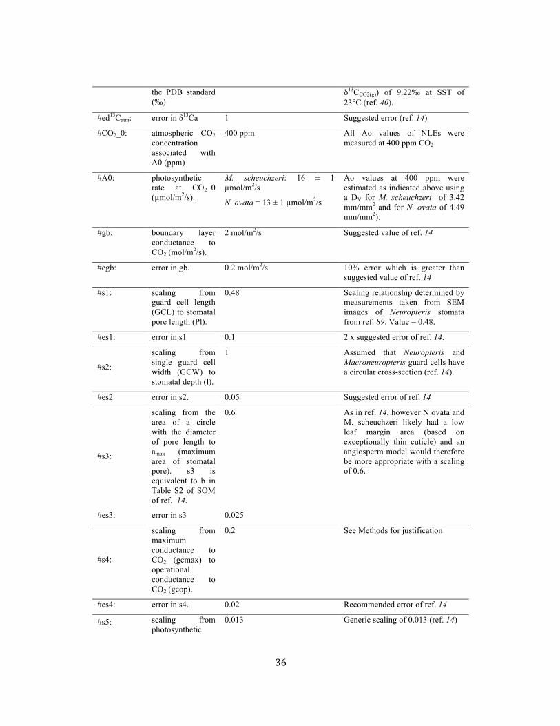
! 36!
the PDB standard (‰)
δ13CCO2(g)) of 9.22‰ at SST of 23°C (ref. 40).
#ed13Catm: error in δ13Ca 1 Suggested error (ref. 14)
#CO2_0: atmospheric CO2 concentration associated with A0 (ppm)
400 ppm All Ao values of NLEs were measured at 400 ppm CO2
#A0: photosynthetic rate at CO2_0 (µmol/m2/s).
M. scheuchzeri: 16 ± 1 µmol/m2/s
N. ovata = 13 ± 1 µmol/m2/s
Ao values at 400 ppm were estimated as indicated above using a DV for M. scheuchzeri of 3.42 mm/mm2 and for N. ovata of 4.49 mm/mm2).
#gb: boundary layer conductance to CO2 (mol/m2/s).
2 mol/m2/s Suggested value of ref. 14
#egb: error in gb. 0.2 mol/m2/s 10% error which is greater than suggested value of ref. 14
#s1: scaling from guard cell length (GCL) to stomatal pore length (Pl).
0.48 Scaling relationship determined by measurements taken from SEM images of Neuropteris stomata from ref. 89. Value = 0.48.
#es1: error in s1 0.1 2 x suggested error of ref. 14.
#s2:
scaling from single guard cell width (GCW) to stomatal depth (l).
1 Assumed that Neuropteris and Macroneuropteris guard cells have a circular cross-section (ref. 14).
#es2 error in s2. 0.05 Suggested error of ref. 14
#s3:
scaling from the area of a circle with the diameter of pore length to amax (maximum area of stomatal pore). s3 is equivalent to b in Table S2 of SOM of ref. 14.
0.6 As in ref. 14, however N ovata and M. scheuchzeri likely had a low leaf margin area (based on exceptionally thin cuticle) and an angiosperm model would therefore be more appropriate with a scaling of 0.6.
#es3: error in s3 0.025
#s4:
scaling from maximum conductance to CO2 (gcmax) to operational conductance to CO2 (gcop).
0.2 See Methods for justification
#es4: error in s4. 0.02 Recommended error of ref. 14
#s5: scaling from photosynthetic
0.013 Generic scaling of 0.013 (ref. 14)
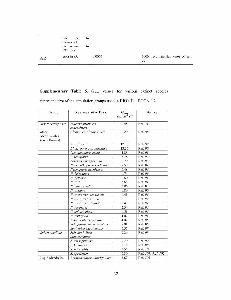
! 37!
rate (A) to mesophyll conductance to CO2 (gm).
#es5: error in s5. 0.0065 100X recommended error of ref. 14
Supplementary Table 5. Gmax values for various extinct species
representative of the simulation groups used in BIOME—BGC v.4.2.
Group Representative Taxa Gmax (mol m-2 s-1)
Source
Macroneuropteris Macroneuropteris scheuchzeri
1.48 Ref. 51
other Medullosales (medullosans)
Alethopteris lesquereuxi 6.29 Ref. 88
A. sullivanti 12.77 Ref. 89 Blanzyopteris praedentata 13.37 Ref. 90 Laveineopteris loshii 4.88 Ref. 91 L. tenuifolia 7.78 Ref. 92 Lescuropteris genuina 1.79 Ref. 93 Neuralethopteris schlehanii 5.57 Ref. 91 Neuropteris aconiensis 0.48 Ref. 94! N. britannica 1.74 Ref. 94! N. flexuosa 1.80 Ref. 94! N. loshii 2.68 Ref. 94! N. macrophylla 0.86 Ref. 94! N. obliqua 1.89 Ref. 90 N. ovata var. aconiensis 1.41 Ref. 94! N. ovata var. sarana 1.13 Ref. 94! N. ovata var. simonii 1.43 Ref. 94! N. rarinervi 2.34 Ref. 94! N. subariculata 1.51 Ref. 94! N. tenuifolia 4.02 Ref. 94! Reticulopteris germarii 4.02 Ref. 95 Schopfiastrum decussatum 5.01 Ref. 96 Senftenbergia plumosa 0.57 Ref. 97 Sphenophyllum Sphenophyllum
apiciserratum 0.26 Ref. 98
S. emarginatum 0.79 Ref. 99 S. koboense 0.18 Ref. 98 S. miravallis 0.54 Ref. 100 S. speciosum 0.30 Ref. 101; Ref. 102 Lepidodendrales Bothrodendron minutifolium 2.67 Ref. 103

! 38!
(lycopsids) B. punctatum 4.44 Ref. 103 Lepidodendron aculeatum 3.53 Ref. 104 L. arberi 3.66 Ref. 104 L. dichotomum 8.15 Ref. 104-105 L. feistmanteli 5.61 Ref. 104 L. loricatum 3.79 Ref. 105 L. mannabachense 2.22 Ref. 104 L. obovatum 4.65 Ref. 105 L. peachii 3.60 Ref. 104 L. rhodianum 1.23 Ref. 104! L. subdichotomum 3.73 Ref. 104! L. veltheimii 2.56 Ref. 104! Lepidophloios acadianus 2.95 Ref. 106! L. acerosus 3.20 Ref. 106! L. grangeri 3.28 Ref. 106! L. laricinus 5.47 Ref. 106! Ulodendron landsburgii 3.44 Ref. 107 U. majus 8.3 Ref. 103 Cordaitales (cordaitaleans)
Cordaabaxicutis boleslawii 1.59 Ref. 108!
C. borassifolioides 4.44 Ref. 108! C. brzyskii 12.05 Ref. 108! C. czeczottensis 4.65 Ref. 108! C. gorae 3.13 Ref. 108! C. papilloborassifolius 6.50 Ref. 108! C. sierszae 2.21 Ref. 108! Cordaadaxicutis bracteatus 0.48 Ref. 108! C. carpaticus 0.09 Ref. 108! C. janinae 0.11 Ref. 108! C. krawjewskae 0.06 Ref. 108! C. laziskae 7.38 Ref. 108! C. pussilostomatus 0.31 Ref. 108! C. tectostomatus 0.06 Ref. 108! C. zalezensis 0.16 Ref. 108! C. zoldanii 0.31 Ref. 108! Cordaites borassifolius 0.14 Ref. 109-110 C. pilsensis 0.57 Ref. 109 C. principalis 1.99 Ref. 111 C. rerichensis 1.62 Ref. 109 Ferns (mostly marattialean tree ferns) Acitheca polymorpha
0.40 Ref. 112
Diplazites unitus 0.07 Ref. 112 Lobatopteris aspidioides 1.05 Ref. 112 L. miltonii 0.35 Ref. 112 L. polypodioides 0.30 Ref. 112 Pecopteris cyathea 0.05 Ref. 112 P. cf. micromiltonii 0.12 Ref. 112 Rumohra adiantiformis 0.07 Ref. 113 Sphaeropteris cooperi 0.26 Ref. 114 Sydneia manleyi 0.27 Ref. 115
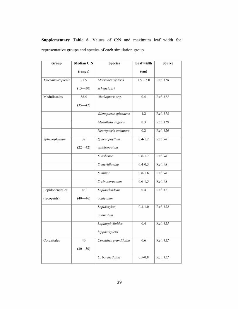
! 39!
Supplementary Table 6. Values of C:N and maximum leaf width for
representative groups and species of each simulation group.
Group Median C:N
(range)
Species Leaf width
(cm)
Source
Macroneuropteris 21.5
(13—30)
Macroneuropteris
scheuchzeri
1.5 – 3.0 Ref. 116
Medullosales 38.5
(35—42)
Alethopteris spp. 0.5 Ref. 117
Glenopteris splendens 1.2 Ref. 118
Medullosa anglica 0.3 Ref. 119
Neuropteris attenuata 0.2 Ref. 120
Sphenophyllum 32
(22—42)
Sphenophyllum
apiciserratum
0.4-1.2 Ref. 98!
S. kobense 0.6-1.7 Ref. 98!
S. meridionale 0.4-0.5 Ref. 98!
S. minor 0.8-1.6 Ref. 98
S. sinocoreanum 0.6-1.5 Ref. 98!
Lepidodendrales
(lycopsids)
43
(40—46)
Lepidodendron
aculeatum
0.4 Ref. 121
Lepidoxylon
anomalum
0.3-1.0 Ref. 122
Lepidophylloides
hippocrepicus
0.4 Ref. 123
Cordaitales 40
(30—50)
Cordaites grandifolius 0.6 Ref. 122
C. borassifolius 0.5-0.8 Ref. 122

! 40!
C. communis 1.5-3.7 Ref. 122
C. diversifolius 1.2-1.5 Ref. 122
C. mansfiedli 1.5 Ref. 122
C. gracilis 0.5 Ref. 122
Ferns (mostly marattialean tree ferns)
31
(20—42)
Corynepteris
cabrierensis
0.2 Ref. 124
Alloiopteris erosa 0.2 Ref. 124
Pecopteris cf. cyathea 0.3 Ref. 125
P. puertollanensis 0.2 Ref. 125
!Supplementary Table 7. Final model parameters for the representative
taxonomic groups used in the BIOME—BGC v.4.2 modeling.
Group Foliar C:N (kg C kg N-1)
SLA (m2 kg C-1)
Gmax (mol m-2 s-1)
Gb (mol m-2 s-1)
Macroneuropteris 21.5 30.3 1.47 1.71 Medullosales 38.5 24.4 2.64 3.46 Sphenophyllum 32.0 22.0 0.49 2.66 Lepidodendrales 43.0 22.8 3.97 3.69 Cordaitales 40.0 23.9 2.29 2.23 Ferns (mostly marattialean tree ferns)
31.0 36.4 0.42 5.41
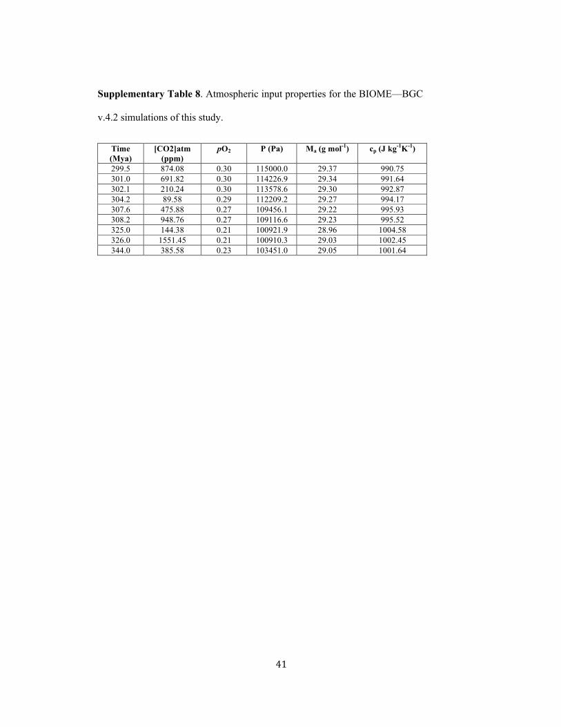
! 41!
Supplementary Table 8. Atmospheric input properties for the BIOME—BGC
v.4.2 simulations of this study.
Time (Mya)
[CO2]atm (ppm)
pO2 P (Pa) Ma (g mol-1) cp (J kg-1K-1)
299.5 874.08 0.30 115000.0 29.37 990.75 301.0 691.82 0.30 114226.9 29.34 991.64 302.1 210.24 0.30 113578.6 29.30 992.87 304.2 89.58 0.29 112209.2 29.27 994.17 307.6 475.88 0.27 109456.1 29.22 995.93 308.2 948.76 0.27 109116.6 29.23 995.52 325.0 144.38 0.21 100921.9 28.96 1004.58 326.0 1551.45 0.21 100910.3 29.03 1002.45 344.0 385.58 0.23 103451.0 29.05 1001.64

! 42!
Supplementary Table 9. Modeled areal extent (%) of select biomes on late Paleozoic land surface.
All results from ref. 6. Horizontal color banding differentiates climate stages (I to IV on
Supplementary Fig. 8). Minimum and maximum values indicated by white and yellow shading,
respectively.
840 ppm 560 ppm
Stage Orbit Interval
Wetland Forest
Tropical Shrubland/Desert &
Barren Land
Tundra Taiga Wetland Forest
Tropical Shrubland/Desert & Barren Land
Tundra Taiga
late interglacial 160 22.6% 21.4% 12.4% 14.5% 24.7% 17.9% 17.9% 12.1% early glacial 165 21.5% 26.4% 3.9% 19.1% 29.8% 22.3% 5.8% 15.6% early glacial 170 21.4% 28.4% 2.7% 15.1% 29.4% 27.2% 3.9% 11.2% peak glacial 175 22.4% 25.8% 2.2% 17.1% 30.7% 24.4% 3.2% 13.4% peak glacial 180 23.3% 21.9% 2.0% 19.3% 30.4% 20.6% 2.7% 16.7% peak glacial 185 22.8% 25.0% 2.1% 19.6% 29.4% 24.5% 2.7% 15.7% peak glacial 190 21.2% 27.1% 2.2% 18.8% 28.0% 26.9% 3.1% 15.4% peak glacial 195 21.0% 26.0% 2.5% 21.5% 28.3% 23.5% 3.7% 17.9% peak glacial 200 20.9% 25.1% 4.5% 20.0% 27.7% 23.9% 4.6% 17.4% peak glacial 205 20.8% 26.2% 3.6% 19.8% 28.2% 24.3% 4.4% 17.3% late glacial 210 21.8% 26.8% 2.3% 19.8% 28.8% 25.4% 3.3% 16.0% late glacial 215 22.3% 25.9% 2.1% 19.2% 29.3% 23.5% 2.9% 16.2% late glacial 220 23.7% 22.3% 1.9% 20.1% 29.9% 20.1% 2.3% 18.0% late glacial 225 22.6% 25.3% 2.2% 20.0% 28.4% 24.9% 2.2% 16.5% deglaciation 230 21.2% 30.3% 2.1% 16.3% 26.0% 30.8% 2.6% 12.6% interglacial 235 20.8% 25.4% 2.5% 19.1% 26.1% 23.1% 2.9% 20.3%
Avg. Interglacial 21.5% 25.7% 5.7% 16.6% 25.6% 24.0% 7.8% 15.0% Avg. early glacial 21.4% 27.4% 3.3% 17.1% 29.6% 24.8% 4.8% 13.4% Avg. peak glacial 21.8% 25.3% 2.7% 19.4% 29.0% 24.1% 3.5% 16.3% Avg. late glacial 22.6% 25.1% 2.2% 19.8% 29.1% 23.5% 2.7% 16.7% Min value 20.8% 21.4% 1.9% 14.5% 24.7% 17.9% 2.2% 11.2% Max value 23.7% 30.3% 12.4% 21.5% 30.7% 30.8% 17.9% 20.3%
Max change 2.9% 8.9% 10.4% 7.0% 6.0% 12.9% 15.7% 9.1%

! 43!
420 ppm 280 ppm
Stage Orbit Interval
Wetland Forest
Tropical Shrubland/Desert &
Barren Land
Tundra Taiga Wetland Forest
Tropical Shrubland/Desert & Barren Land
Tundra Taiga
late interglacial 160 38.8% 18.4% 10.1% 9.2% 47.1% 21.9% 5.9% 8.1% early glacial 165 43.3% 21.8% 5.0% 10.4% 49.2% 24.3% 3.6% 8.4% early glacial 170 41.8% 25.5% 3.6% 8.9% 49.2% 26.1% 3.3% 7.9% peak glacial 175 43.7% 21.5% 3.8% 9.2% 49.7% 23.5% 3.2% 8.1% peak glacial 180 43.2% 21.4% 4.2% 9.6% 49.9% 22.5% 3.0% 8.1% peak glacial 185 44.1% 22.1% 3.4% 9.6% 49.4% 23.7% 3.1% 8.3% peak glacial 190 43.1% 23.3% 4.1% 9.3% 49.7% 24.2% 3.2% 8.4% peak glacial 195 42.7% 23.1% 4.5% 9.6% 49.2% 23.5% 4.0% 9.0% peak glacial 200 43.1% 22.8% 5.6% 9.5% 48.9% 23.2% 4.5% 8.5% peak glacial 205 44.0% 21.8% 4.9% 9.2% 49.1% 24.1% 4.3% 8.5% late glacial 210 44.6% 23.1% 3.8% 8.7% 49.6% 24.3% 3.4% 8.9% late glacial 215 45.6% 21.1% 3.6% 8.5% 49.5% 23.9% 3.2% 8.4% late glacial 220 45.1% 20.5% 3.5% 8.9% 48.6% 22.7% 3.1% 8.4% late glacial 225 45.4% 21.4% 3.4% 8.7% 49.2% 24.7% 3.5% 7.7% deglaciation 230 44.7% 24.5% 2.9% 7.5% 48.9% 26.0% 3.3% 7.6% interglacial 235 44.6% 21.2% 4.3% 8.6% 50.1% 22.8% 3.8% 7.8%
Avg. Interglacial 42.7% 21.4% 5.8% 8.4% 48.7% 23.4% 4.3% 7.8% Avg. early glacial 42.6% 23.6% 4.3% 9.6% 49.2% 25.2% 3.5% 8.2% Avg. peak glacial 43.4% 22.4% 4.4% 9.4% 49.4% 23.5% 3.6% 8.4% Avg. late glacial 45.2% 21.5% 3.6% 8.7% 49.2% 23.9% 3.3% 8.4% Min value 38.8% 18.4% 2.9% 7.5% 47.1% 21.9% 3.0% 7.6% Max value 45.6% 25.5% 10.1% 10.4% 50.1% 26.1% 5.9% 9.0% Max change 6.7% 7.1% 7.2% 2.9% 3.0% 4.2% 2.9% 1.5%