Letter N-Gram-based Input Encodingfor

Continuous Space Language Models

Diploma Thesis of

Henning Sperr

At the Department of InformaticsInstitute for Anthropomatics

Reviewer: Prof. Dr. Alexander WaibelSecond reviewer: Dr. Sebastian StükerAdvisor: Dipl. Inform. Jan Niehues

Duration: 01 January 2013 – 30 June 2013

KIT – University of the State of Baden-Wuerttemberg and National Research Center of the Helmholtz Association www.kit.edu

I declare that I have developed and written the enclosed thesis completely by myself, andhave not used sources or means without declaration in the text.

Karlsruhe, 21.06.2013

. . . . . . . . . . . . . . . . . . . . . . . . . . . . . . . . . . . . . . . . .(Sperr, Henning)

Zusammenfassung

In dieser Arbeit prasentieren wir eine neue Eingabeschicht fur Neuronale Netzwerk Sprach-modelle, sowie einen Entwurf fur ein Deep Belief Network -Sprachmodell. Ein großes Prob-lem der normalerweise genutzten Wortindex-Eingabeschicht ist der Umgang mit Wortern,die zuvor in den Trainingsdaten nicht vorkamen. Bei manchen Neuronale Netzwerk Ar-chitekturen muss die Große des Eingabevokabulars auf Grund der Komplexitat und Rechen-zeit eingeschrankt und somit die zusatzliche Menge der unbekannten Worter vergroßertwerden. Diese Netzwerke mussen auf ein normales N-Gram Sprachmodell zuruckgreifenum dennoch eine Wahrscheinlichkeit zu liefern. Bei einer anderen Methode reprasentiertein Neuron in der Eingabeschicht alle ungesehenen Worter.

In der neuen Letter N-Gram Eingabeschicht wird dieses Problem behoben, indem wirWorte als Teilworte reprasentieren. Mit diesem Ansatz haben Worter mit ahnlichen Buch-staben auch ahnliche Reprasentationen in der Eingabeschicht des Neuronalen Netzwerks.Wir wollen zeigen, dass es damit moglich ist fur unbekannte Worter dennoch sinnvolleSchatzungen abzugeben sowie morphologische Informationen eines Wortes zu erfassen, dadiese Formen eines Wortes dennoch haufig die selben Buchstabenfolgen enthalten. Wirzeigen die Auswirkung im Bereich der statistischen maschinellen Ubersetzung mithilfeeines Neuronalen Netzwerkes basierend auf restricted Boltzmann machines.

Wir benutzen diese Boltzmann-Maschinenarchitektur ebenfalls um die Gewichte des DeepBelief Networks zuvor zu trainieren und diese danach mit dem Contrastive Wake Sleep-Algorithmus abzustimmen. Fur dieses Deep Belief Network haben wir eine Architekturgewahlt, die vorher bereits bei handgeschriebener Zi↵ernerkennung gute Resultate erzielenkonnte.

Wir untersuchen die Ubersetzungsqualitat sowie die Trainingszeit und unbekannte Wor-trate bei einer Deutsch nach Englisch Ubersetzungsaufgabe, welche die TED Daten be-nutzt. Wir benutzen die selben Systeme und untersuchen wie gut sie auf eine anderendomanenverwandten Aufgabe, namlich Universitatsvorlesungen, generalisieren. Außerdemhaben wir Experimente vom Englisch nach Deutsch auf Nachrichtentexten durchgefurt.Um die Systeme zu vergleichen benutzen wir die BLEU Metrik. Wir zeigen, dass mit derneuen Eingabeschicht eine Verbesserung von bis zu 1.1 Punkten erzielt werden kann. DieDeep Belief Network Architektur war in der Lage das Vergleichssystem ohne zusatzlichesSprachmodell um bis zu 0.88 Punkte zu verbessern.

iii

Abstract

In this thesis we present an input layer for continuous space language models, as well as alayout for a deep belief network language model. A big problem of the commonly used wordindex input layer is the handling of words that have never been seen in the training data.There are also neural network layouts where the vocabulary size has to be limited due to theproblem of complexity and computation time. These networks have to back-o↵ to normaln-gram language models or use a neuron for all unknown words. With our new lettern-gram input layer this problem can be solved by modeling each word as a combinationof subword features. With this approach words containing similar letter combinationswill have close representations. We think this will improve the out-of-vocabulary rate aswell as capturing morphological information about the words, since related words usuallycontain similar letters. We show their influence in the task of machine translation using acontinuous space language model based on restricted Boltzmann machines.

We also used this Boltzmann machine architecture to pretrain the weights for a deep beliefnetwork and afterwards fine-tuning the system using the contrastive wake-sleep algorithm.For our deep belief network we chose a layout that proved to be able to do handwritten digitrecognition. We evaluate the translation quality as well as the training time and out-of-vocabulary rates on a German-to-English translation task of TED and university lecturesas well as on the news translation task translating from English-to-German. The systemswere compared according to their BLEU scores. Using our new input layer approach again in BLEU score by up to 1.1 BLEU points can be achieved. The deep belief networkarchitecture was able to improve the baseline system by about 0.88 BLEU points.

v

Contents

1. Introduction 1

1.1. Language Modeling . . . . . . . . . . . . . . . . . . . . . . . . . . . . . . . . 21.2. Overview . . . . . . . . . . . . . . . . . . . . . . . . . . . . . . . . . . . . . 4

2. Previous Work 5

3. Neural Networks 7

3.1. Feed Forward Neural Networks . . . . . . . . . . . . . . . . . . . . . . . . . 83.1.1. Training . . . . . . . . . . . . . . . . . . . . . . . . . . . . . . . . . . 8

3.2. Boltzmann Machines . . . . . . . . . . . . . . . . . . . . . . . . . . . . . . . 93.2.1. Restricted Boltzmann Machines . . . . . . . . . . . . . . . . . . . . . 93.2.2. Contrastive Divergence Learning . . . . . . . . . . . . . . . . . . . . 11

3.3. Deep Neural Networks . . . . . . . . . . . . . . . . . . . . . . . . . . . . . . 113.3.1. Training . . . . . . . . . . . . . . . . . . . . . . . . . . . . . . . . . . 133.3.2. Contrastive Wake-Sleep Fine Tuning . . . . . . . . . . . . . . . . . . 13

4. Continuous Space Language Models 15

4.1. Feed Forward Language Model . . . . . . . . . . . . . . . . . . . . . . . . . 154.2. Restricted Boltzmann Machine Language Model . . . . . . . . . . . . . . . 16

5. Letter-based Word Encoding 19

5.1. Motivation . . . . . . . . . . . . . . . . . . . . . . . . . . . . . . . . . . . . 195.2. Features . . . . . . . . . . . . . . . . . . . . . . . . . . . . . . . . . . . . . . 19

5.2.1. Additional Information . . . . . . . . . . . . . . . . . . . . . . . . . 215.2.2. Tree-Split Features . . . . . . . . . . . . . . . . . . . . . . . . . . . . 21

6. Deep Belief Network Language Model 25

7. Implementation 27

7.1. Design . . . . . . . . . . . . . . . . . . . . . . . . . . . . . . . . . . . . . . . 277.2. Visual Debugging . . . . . . . . . . . . . . . . . . . . . . . . . . . . . . . . . 29

8. Evaluation 33

8.1. Word Representation . . . . . . . . . . . . . . . . . . . . . . . . . . . . . . . 338.2. Translation System Description . . . . . . . . . . . . . . . . . . . . . . . . . 348.3. German-to-English TED Task . . . . . . . . . . . . . . . . . . . . . . . . . . 35

8.3.1. Caps Feature . . . . . . . . . . . . . . . . . . . . . . . . . . . . . . . 368.3.2. Tree-Split Feature . . . . . . . . . . . . . . . . . . . . . . . . . . . . 388.3.3. Iterations . . . . . . . . . . . . . . . . . . . . . . . . . . . . . . . . . 408.3.4. Hidden Size . . . . . . . . . . . . . . . . . . . . . . . . . . . . . . . . 418.3.5. Combination of Models . . . . . . . . . . . . . . . . . . . . . . . . . 418.3.6. Deep Belief Models . . . . . . . . . . . . . . . . . . . . . . . . . . . . 428.3.7. Unknown Words . . . . . . . . . . . . . . . . . . . . . . . . . . . . . 42

vii

viii Contents

8.4. German-to-English CSL Task . . . . . . . . . . . . . . . . . . . . . . . . . . 448.5. English-to-German News Task . . . . . . . . . . . . . . . . . . . . . . . . . 458.6. English-to-French TED Task . . . . . . . . . . . . . . . . . . . . . . . . . . 468.7. Model Size and Training Times . . . . . . . . . . . . . . . . . . . . . . . . . 46

9. Future Work & Conclusion 49

Bibliography 51

Appendix 55

A. Complete Tables for each Task . . . . . . . . . . . . . . . . . . . . . . . . . 55

viii

1. Introduction

In today’s society cultural exchange becomes more important every day. The means oftransportation and communication developed very fast over the last sixty years, so that noweveryone is able to access huge amounts of information over the Internet or by travellingabroad. In this more and more globalised world the cultural and social borders of di↵erentcountries grow closer together and make it necessary to speak or understand multiple lan-guages.For example in politics where communication between countries is crucial to maintainpeace and understanding. If the translators provide false or bad translations the relationbetween two countries could become tense. In the European Parliament there are simul-taneous translations for each nation. Everyone can hold a speech in his mother tongueand the audience can listen to the simultaneous translations in their mother tongue. Thisis also a very stressful task for humans since simultaneous translations require big e↵ortand concentration and usually people work in teams and change shift in regular intervals.

Another area where multilingualism gains importance is the workplace, where often teamscontain people from all over the world. Good communication is necessary to have a wellfunctioning and productive work environment. Often English is considered to be thecommon spoken language not all people speak or understand it. Especially when travelingto di↵erent countries people in rural areas are not necessarily able to speak English. It isalso not possible for everyone to learn three or more languages so there is an increasingneed for translations. Professional human translation is expensive and sometimes notpossible, especially for languages with very few speakers. That is why machine translationis an important field of research.

Computers are all around us in our daily life and being always connected to the Internetbecomes more and more common. With the recent increase in smartphones, people are ableto use machine translation software everywhere1 2. This has many private applications,for example being able to ask for things or order in a restaurant during travel. But alsoin political area, where for example U.S. soldiers on a mission could translate from andto Arabic, to talk to local people during a mission. Another important task for mobilemachine translation is for doctors that go abroad in third world countries to help, but donot speak the local languages. It is important to have good communication so the doctoris able to find the best way to cure the patient.

1http://www.jibbigo.com/website/2http://www.google.de/mobile/translate/

1

2 1. Introduction

Another important task is to make knowledge available to everyone. To do this, projectslike Wikipedia or TED try to accumulate information, in many di↵erent languages, thatis freely available for everybody. There is a big need, especially for science and research,to share results and knowledge through the Internet and across language borders. Thenumber of universities that provide open lectures or video lectures online is growing andwith this the need to automatically translate these lectures into di↵erent languages.

State of the art machine translation systems are good at doing domain limited tasks forclose languages e.g. English-French, the performance is much worse for broad domain andvery di↵erent languages e.g. English-Japanese. But even for close languages the translationquality for broad domain translation systems is still not on a professional level.

1.1. Language Modeling

State of the art systems use phrase-based statistical machine translation (SMT). The ideais to take parallel data to train the most probable translations from one language into theother. Phrases which consist of one or more words are extracted from an alignment, whichusually is generated by taking the most probable word alignments from all the parallelsentences. These phrases are then stored in a phrase table and during decoding time usedto translate chunks from the source language into the target language. This is a hard tasksince the number of possible translations grows exponentially.

The components used by such an SMT system can be described using the Bayes-Theoremwhich is

P (e|f) = P (f |e) · P (e)

P (f)(1.1)

Where P (e|f) is the probability that sentence e is the translation for the given sentence f .This equals P (f |e) the likelihood function, which is the probability of the sentence giventhe translation hypothesis. The probability of the translated sentence P (e), is how likelyit is that the translation hypothesis is a good sentence of the target language. This isdivided by P (f), the probability of the source sentence, which is usually omitted since itis constant for every sentence. The goal now is to find a sentence e so that this probabilityP (e|f) is maximized rewriting above formula as

argmaxe

P (e|f) = argmaxe

P (f |e) · P (e) (1.2)

By doing so, the interesting components for optimization are the decoding process whichequals finding the e with the maximum probability, the translation model which assignsthe probability P (f |e) to sentence pairs and the language model P (e).

It is important to have a language model, since words can have many di↵erent translationsin the target language and there needs to be a way to decide which is the best translationgiven a certain context. If only the translation model probabilities would be used forexample, the most probable English translation for the German word “Bank” is “bank”. Itwould never be translated into “bench” which is another valid translation, depending ontext context. Phrase-based translation compared to word-based translation helps solvingthis problem because words can be translated in context if the phrase has been seen duringtraining, but this is not able to solve the problem entirely. Even with phrases there is stillhave no context information in between the phrase boundaries. The translation hypothesismight be very influent. By training a model that can assign a probability to a sentence, orparts of a sentence, a better estimate for translations using di↵erent contextual information

2

1.1. Language Modeling 3

can be obtained. During decoding time di↵erent pruning methods are used, due to theexponential growth of the search tree. Often, very improbable hypothesis will be cut o↵and a language model is one of the features that helps to evaluate whether the currenthypothesis can be cut o↵ or should be kept. Since the probability of a whole sentence,P (W ) is hard to estimate, because most of the sentences appear only once in the trainingdata, a di↵erent approach is used. This approach is called n-gram-based language model,where the probability of a word given a limited history of words is calculated with

P (wn

1

) = P (w1

)nY

i=2

P (wi

|wi�1

1

) (1.3)

Where wi

1

is a word sequence w1

, ..., w

i

and w

i

is the i-th word. A good statistical languagemodel should assign a non-zero probability to all possible word strings wn

1

but in practicethere are several problems with the typical n-gram-based approach. One is that if theparameter N is too big, data sparseness will be a problem and there will be lots of n-gramsthat have no or very little statistical data. This means that di↵erent back-o↵ or smoothingtechniques have to be used to get a nonzero probability for those n-grams. If N is chosentoo small, not enough context is captured to make meaningful distinctions. For exampleby using only unigram probabilities the model will give no information about fluency ortranslations in context. To deal with the data sparseness problems several approaches havebeen developed to calculate probabilities for unseen events. One example would be backingo↵ to lower order n-grams [Kat87] under certain circumstances. The most common usedtechnique today is called modified Kneser-Ney smoothing [KN95,CG96]. It is essentiallya back-o↵ interpolation algorithm with modified unigram probabilities.

In these standard back-o↵ n-gram language models the words are represented in a discretespace, which prevents true interpolation of the probabilities for the unseen n-grams. Thismeans that if the position in our discrete word space is changed it will lead to a discontinu-ous change in the n-gram probability. In this work we try to explore the use of continuousspace language models (See Bengio et al. [BDVJ03]) to get a better approximate for n-grams that were never seen before. For this we developed new input layers for the restrictedBoltzmann machine Language Model (RBMLM) of Niehues and Waibel [NW12] that tryto capture morphological information of words by using di↵erent subword features. Wetry to overcome the problem of out-of-vocabulary (OOV) words by using subword featuresthat will yield a good indicator for words that have the same function inside the sentence.The subword feature approach has the advantage that for big vocabularies the input layerbecome smaller and with that the training time of the network decreases.

Another part ot this work will be the exploration, whether so called Deep Belief Networks(DBNs), which proved to be good as acoustic models in speech recognition and digit imagerecognition [HDY+12,rMDH12], are also useful in inferring the most probable n-gram. Inthe handwritten digit image recognition task (MINST) deep models achieved improvementsover state of the art support vector machines in classifying di↵erent digits. In the speechrecognition task a similar layout was used to project the cepstral coe�cients of a contextof frames onto the continuous space and use this vector to predict the hidden Markovmodel state. In our work, we try to project the history of a word through multiple layersand see if this higher order representation can model additional information that is usefulto predict the probability of the current word. For this we took the design that Hinton etal. [HOT06] used for digit recognition on the MINST handwritten digit database.

3

4 1. Introduction

1.2. Overview

The rest of this thesis is structured as follows:

In Chapter 2 we will give an overview of the field of neural networks and language model-ing using continuous space representations. After discussing di↵erent approaches tothe topic we want to contrast the work done in this thesis with work that has beendone before.

In Chapter 3 the basics of neural networks that are needed to understand the work donein this thesis will be presented. We will explain basic feed forward neural networksand the di↵erence to Boltzmann machines. We will explain how restricted Boltzmannmachines are used to pretrain deep neural networks and introduce an algorithm thatwill be used for the fine-tuning of this model.

In Chapter 4 we will introduce two basic continuous space language modeling approachesand how they try to infer probabilities for a word n-gram. We will also explain incase of the restricted Boltzmann machine, how the 1-in-n coding word index works.

In Chapter 5 we will motivate the proposed input layer and introduce additional featuresthat can be used with the new input layer.

In Chapter 6 we will give a brief introduction to the deep belief network language modellayout that we propose in this thesis. We will explain on why we decided to usethe given layout and explain how the probabilities are going to be inferred from thisnetwork.

In Chapter 7 we will talk about the design of the implementation and explain a few meth-ods that helped while debugging the code and how to visually check if learning isworking well or not.

In Chapter 8 we will explain on which systems we tested our models and describe theoutcome of di↵erent experiments. We will explore if the input layer proposed in thiswork achieves better performance then earlier proposed methods and do experimentson di↵erent improvements of the input layer.

In Chapter 9 we will conclude our work and give an outlook over future work that can bedone to further enhance this research.

4

2. Previous Work

Research about neural networks in natural language processing dates back into the 1990swhere for example Waibel et al. [WHH+90] used time delay neural networks to improvespeech recognition quality. Gallant [Gal91] used neural networks to resolve word sense dis-ambiguations. Neural networks were also used as part-of-speech tagger in Schmid [Sch94a].One of the first approaches to use them in language modeling was in Nakamura andShikano [NMKS90], where a neural network was used to predict word categories. Miiku-lainen and Dyer researched another approach to continuous natural language processingbased on hierarchically organized subnetworks with a central lexicon [MD91].

At that time the vast computational resources were not available so that, after a shortrecession, now in recent times new neural network approaches have come up again. Xuand Rudnicky [XR00] proposed a language model that has an input consisting of one wordand no hidden units. This network was limited to infer unigram and bigram statistics.One of the first continuous space language models that paved the way for methods thatare used today was presented in Bengio et al. [BDVJ03]. They used a feed forward multi-layer perceptron as n-gram language model and achieved a decrease in perplexity between10 and 20 percent. In Schwenk and Gauvain [SG05] and later in Schwenk [Sch07] re-search was performed on training large scale neural network language models on millionsof words resulting in a decrease of the word error rate for continuous speech recognition. InSchwenk [Sch10] they use the continuous space language modeling framework to re-scoren-best lists of a machine translation system during tuning. Usually these networks useshort lists to reduce the size of the output layer and to make calculation feasible. Therehave been approaches to optimize the output layer of such a network, so that vocabulariesof arbitrary size can be used and there is no need to back o↵ to a smaller n-gram model Leet al. [LOM+11]. In this Structured Output Layer (SOUL) neural network language modela hierarchical output layer was chosen. Recurrent neural networks have also been usedto try and improve language model perplexities in Mikolov et al. [MKB+10], concludingthat Recurrent neural networks potentially improve over classical n-gram language modelswith increasing data and a big enough hidden unit size of the model. In the work of Mnihand Hinton [MH07] and Mnih [Mni10] training factored restricted Boltzmann machinesyielded no gain compared to Kneser-Ney smoothed n-gram models. But it has been shownin Niehues and Waibel [NW12], that using a restricted Boltzmann machine with a di↵erentlayout during decoding can yield an increase in BLEU score.

There has also been research in the field of using subword units for language modeling.In Shaik et al. [SMSN11] linguistically motivated sub-lexical units were proposed to im-

5

6 2. Previous Work

prove open vocabulary speech recognition for German. Research on morphology-basedand subword language models on a Turkish speech recognition task has been done by Saket al. [SSG10]. The idea for Factored Language models in machine translation has beenintroduced by Kirchho↵ and Yang [KY05]. Similar approaches to develop joint languagemodels for morphologically rich languages in machine translation have been presented bySarikaya and Deng [SD07].In Emami et al. [EZM08] a factored neural network languagemodel for Arabic language was built. They used di↵erent features such as segmentation,part-of-speech and diacritics to enrich the information for each word. We are also goingto investigate, if a deep belief network trained like described in Hinton et al. [HOT06] canget a similar good performance as in image recognition and acoustic modeling. For thiswe use Boltzmann machines to do layer by layer pretraining of a deep belief network andafter that wake-sleep fine-tuning to find the final parameters of the network. To the bestof our knowledge using a restricted Boltzmann machine with subword input vectors tocapture morphology information is a new approach and has never been done before. Theapproach to project words on a continuous space through multiple layers and use the toplevel associative memory to sample the free energy of a word given the continuous spacevector has as far as we know not been done yet.

6

3. Neural Networks

A neural network is a mathematical model, which tries to represent data in the same waythe human brain does. It consists of neurons that are connected with each other and usinglearning techniques the connections between di↵erent neurons strengthen or weaken. Theweights of these connections determine how much a neuron that activates influences theneurons that are connected to it. It is often used to model complex relations and findpatterns in data.

Neural networks were originally developed in 1943 by Warren McCulloch and Walter Pitts.They elaborated on how neurons might work and they modeled a simple network withelectrical circuits. In 1949 Donald Hebb pointed out in his book ”The Organization ofBehavior” that neural pathways that are often used get stronger, which is a crucial part tounderstand human learning. During the 1950’s with the rise of von Neumann computersthe interest in neural networks decreased until in 1958 Frank Rosenblatt came up withthe perceptron, which led to a reemerge of the field. Soon after that in 1969 Minsky andPapert wrote a book on the limitations of the perceptron and multilayer systems, whichled to a significant shortage in funding for the field. In 1974 Paul Werbos developed theback-propagation learning method, which was simultaneously rediscovered in 1985-1986by Rumelhart and McClelland and is now probably the most well known and widely usedform of learning today.

Recently neural networks are regaining attention since the advancement in informationtechnology and the development of new methods makes training deep neural networksfeasible. The term deep belief network describes a generative model that is composedof multiple hidden layers. It is possible to have many di↵erent layouts of the neuronsand connections in such a network and one of the most common layouts is similar tothe feed forward network (See Figure 3.1). In a feed forward network we have an inputlayer representing the data we want to classify. After that we can have one or multiplehidden layers until we reach the output layer which will contain the feature vector for thegiven input data. Another common layout is the recurrent neural network in which theconnections of the units form a directed circle. This allows to capture dynamic temporalbehavior.

7

8 3. Neural Networks

Input Hidden Layers Output

Figure 3.1.: Example for a feed forward neural network.

3.1. Feed Forward Neural Networks

A typical feed forward network consists of an input layer, one or many hidden layers andan output layer. The decision if a neuron turns on or o↵ is usually chosen by summingthe input of the neurons in the layer below, which is either on or o↵ for binary neuronsmultiplied by the weight of the connection and a sigmoid activation function (Figure 3.2).This way the data is represented by the input neurons and propagated through the weightsinto the hidden layer until the output layer. The logistic sigmoid function is defined as

p(Ni

= on) =1

1 + e�t

(3.1)

where N

i

is the ith neuron and t is the input from other neurons. Usually a threshold isset to decide whether the neuron turns on or o↵. In some training algorithms though, asampling strategy is used to sometimes accept improbable samples (e.g. a high probabilityneuron not turning on) to get a random walk over the trainings surface and not get stuckin local optima.

Figure 3.2.: Sigmoid activity function.1

3.1.1. Training

Training a neural network is a di�cult task. There are three major paradigms for thelearning task.

1Source: http://en.wikipedia.org/wiki/Sigmoid_function

8

3.2. Boltzmann Machines 9

1. In Supervised Learning we have a set of data and the corresponding classes and wetry to change the parameters of the model in a way that the data gets classifiedcorrectly. A cost function is used to determine the error between correct labels andnetwork output.

2. In Unsupervised Learning we have only data without labels and need to define a costfunction that measures the error given the data and the mapping of our network.

3. In Reinforcement Learning we think of the problem as a Markov decision process,where we have several states and in each of these states we have probabilities of goinginto one of the other states. For each of these transitions a reward or punishment isgiven according to the output. In this way we try to learn the best transition weightsand probabilities to get a good model.

The most commonly used algorithm is a supervised learning method called back-propagation.In this algorithm examples are shown to the network and the output of the neural net-work is compared with the expected output. The motivation for this algorithm is that achild learns to recognize things by seeing or hearing many examples an getting “labels”from other people who tell the child what it is seeing. Having enough data and labelsshallow neural networks can be trained very well using this algorithm. Commonly theweights are initialized randomly and trained for some iterations. The big problem withrandom weights and deep networks is that back-propagation tends to settle in very badlocal minima. There are di↵erent approaches to cope with this problem, for example usingSimulated Annealing techniques. In this work we will not initialize the weights randomlybut use a restricted Boltzmann machine to pretrain the weights of a deep belief network.Another problem in training deep networks with back-propagation is a phenomenon calledexplaining away. This will be further described in the Chapter 6.1.

3.2. Boltzmann Machines

A Boltzmann machine is a type of stochastic recurrent neural network in which there are anumber of neurons that have undirected symmetric connections with every other neuron.Such a network with five neurons can be seen in Figure 3.3.

Figure 3.3.: Example for a Boltzmann machine having five neurons.

Since learning in a normal Boltzmann machine with unrestricted connections is di�cultand time consuming often restricted Boltzmann machines are used instead.

3.2.1. Restricted Boltzmann Machines

In a restricted Boltzmann machine an additional constraint is imposed on the model. Wehave no connections in the hidden and visible layer. This means that a visible node hasonly connections to hidden nodes and hidden nodes only to visible nodes (Figure 3.4 )

9

10 3. Neural Networks

Visible

Hidden

Figure 3.4.: Example for a restricted Boltzmann machine with three hidden units and twovisible units.

The restricted Boltzmann machine is an energy-based model that associates an energy toeach configuration of neuron states. Through training we try to give good configurationslow energy and bad configurations high energy. Since we try to infer ”hidden” features inour data we will have some neurons that correspond to visible inputs and some neuronsthat correspond to hidden features. We try to learn good weights and biases for thesehidden neurons during training and we hope that they are able to capture higher leveldata.

The Boltzmann machine assigns the energy according to the following formula

E(v, h) = �X

i2visiblea

i

v

i

�X

j2hiddenb

j

h

j

�X

(i,j)2(visible,hidden)

v

i

h

j

w

ij

(3.2)

where v and h are visible and hidden configurations and w

i,j

is the weight between unit iand j. Given this Energy Function we assign the probability in such a network as

p(v, h) =1

Z

e�E(v,h) (3.3)

with the partition function Z as

Z =X

v,h

e�E(v,h) (3.4)

where v and h are visible and hidden configurations. Since we are interested in the prob-ability of our visible input we can marginalize Equation 3.3 over the hidden units andget

p(v) =1

Z

X

h

e�E(v,h)

. (3.5)

Usually the partition function Z is not feasible to compute since it is a sum over allpossible visible and hidden configurations. To overcome this problem we will not usethe probability of our visible input but something called free energy. The free energy ofa visible configuration in a restricted Boltzmann machine with binary stochastic hiddenunits is defined as

F (v) = �X

i

v

i

a

i

�X

j

log(1 + exj ) (3.6)

10

3.3. Deep Neural Networks 11

with x

j

= b

j

+P

i

v

i

w

ij

. It can also be shown that

e�F (v) =X

h

e�E(v,h)

. (3.7)

Inserting this into Equation 3.5 we get

p(v) =1

Z

e�F (v)

. (3.8)

This formula still contains the partition function but we also know that the free energywill be proportional to the true probability of our visible vector.

3.2.2. Contrastive Divergence Learning

For this work we used Contrastive Divergence learning as proposed in Hinton [Hin02]. Itis an unsupervised learning algorithm that uses Gibbs-Sampling. The implementation isbased on Hinton [Hin10]. In order to do this, we need to calculate the derivation of theprobability of the example given the weights:

� log p(v)

�w

ij

= <v

i

h

j

>

data

�<v

i

h

j

>

model

(3.9)

where <v

i

h

j

>

model

is the expected value of vi

h

j

given the distribution of the model. Inother words we calculate the expectation of how often v

i

and h

j

are activated together giventhe distribution of the data, minus the expectation of them being activated together giventhe distribution of the model, which will be calculated using Gibbs-Sampling techniques.The first part is easy to calculate since we just input the data and propagate the activationsinto the hidden units and count which of the pairs are on together and which are o↵. Forthe estimation of <v

i

h

j

>

model

usually many steps of Gibbs-Sampling are necessary toget an unbiased sample from the distribution. This can be seen in Figure 3.5 where thegreen units depict the activation of the data and the red units are the so called fantasyparticles inferred from the distribution of the model. The common implementation of theContrastive Divergence algorithm only performs one step of sampling. Minimizing thisContrastive Divergence function works well as shown in several experiments. [Hin02,CPH].

j j j

i i i

vihj (0) vihj (1) vihj (1)

Figure 3.5.: Markov Chain of the Contrastive Divergence learning step.

3.3. Deep Neural Networks

In recent times deep neural network language models are beginning to gain importance,since they achieved good results in speech recognition and image recognition tasks. With

11

12 3. Neural Networks

increasing computational power training large neural networks with multiple hidden layersbecomes more and more feasible. Despite that it is still hard to train many hidden layersof a directed belief network using back-propagation. Especially when the weights arerandomly initialized the algorithm will easily get stuck in local optima. Inference in deepdirected neuronal networks having many hidden layers is di�cult, due to the problem of“explaining away”. A common example2 for the problem can be seen in Figure 3.6. Thetwo independent causes for the jumping house become highly dependent when we see thehouse jumping. The weights of the arrows coming from the outside represent the bias andin case of the earthquake node �10 means that without any other input the node is e10

times more likely to be o↵ then on. If we now observe that the earthquake node is on andthe truck node is o↵ the total input of the jumping house node is zero which means thatthe node will turn on half of the time. This is a much better explanation that the housejumped than the probability of e�20 we get when earthquake and truck node are o↵, whichwould mean the house jumped on its own. It is also unlikely to turn on both the earthquakeand the truck node since the likelihood for that happening is also e�10 · e�10 = e�20. If wenow want to know the probability of the truck hitting the house, when we know the housejumps the probability changes whether the earthquake node is turned on or o↵. Whenthe earthquake node is turned on it “explains away” the evidence for the truck hittingthe house. This problem happens when we have several hidden unobserved neurons thatinfluence each other.

earth-quake

truck hits

house

house jumps

-20

-10 -10

+20+20

Figure 3.6.: Example for “explaining away” in a directed deep neuronal network.

There are Markov chain Monte Carlo methods [Nea92] which try to cope with this problembut they are usually very time consuming. In Hinton et al. [HOT06] they used complemen-tary priors to eliminate the explaining away e↵ect using a greedy layer wise training withrestricted Boltzmann machines. In our work we will use a so called deep belief network(e.g. Figure 3.7), which is a probabilistic generative model. It is composed of an inputlayer and several hidden layers. These hidden layers are typically binary and the top twolayers have undirected symmetric connections which form a so called associative memory.

2This example is taken from Hinton et al. [HOT06]

12

3.3. Deep Neural Networks 13

OutputLayer

HiddenLayer

Inputlayer

HiddenLayer

...

Figure 3.7.: Layout of a deep belief network.

3.3.1. Training

The training of a deep belief network will be greedy layer wise following these steps:

1. Train the first layer as an RBM that models the distribution P (h0|x) of the firsthidden layer h0 given the data x.

2. Use the first layer to obtain a representation of the input and use this as data forthe second layer to calculate P (h1|h0). We will use the real valued activations fromthe lower level hidden activities. We then use this data to train the next layer RBM.

3. We repeat 1. and 2. for the desired number of layers.

4. The last step can be fine-tuning the connections in between the layers since afterpretraining we have a good initialization for algorithms like back-propagation or thewake-sleep algorithm

Each of the RBMs will be trained separately. If the number of weights of a preceding layeris the same as in the current layer we will initialize the weights from the layer below insteadof using random values. When we pretrained each layer using the Contrastive Divergencealgorithm, the weights of the layers already have a good initialization to classify the data.But since the layers were trained independently the transition from one layer to the nextcan be improved by using a fine-tuning algorithm. This can usually be back-propagationor in our case the contrastive wake-sleep algorithm as described in Hinton et al. [HOT06].

3.3.2. Contrastive Wake-Sleep Fine Tuning

Contrastive wake-sleep fine-tuning is an unsupervised algorithm to fine tune a deep beliefnetwork. For this algorithm the weights and biases of the network will be split up intogenerative weights (top-down weights) and recognition weights (bottom-up weights). Thealgorithm itself consists of two phases namely the wake and sleep phase. During the wakephase the data is propagated bottom up through the network where the binary featurevectors of one layer are used as data for the next. The top level associative memory layeris then trained with a few steps of Contrastive Divergence training. This wake phase can

13

14 3. Neural Networks

be seen as the model observing the real data. The Contrastive Divergence learning inthe associative memory can be seen as the process of dreaming, where the reconstructionsobtained using Gibbs sampling represent what the model likes the data to look like. Thisreconstructed vector is then propagated back down into the input layer in the so calledsleep phase. These vectors obtained during the wake and sleep phase are used to trainthe recognition and generative weights in a way to better represent the data. For moreinformation and a pseudo-code implementation of this algorithms please refer to Hintonet al. [HOT06].

14

4. Continuous Space Language Models

In this chapter we will take a brief look at di↵erent continuous space language modelapproaches that have been introduced in the past. We will introduce one feed forwardlanguage model approach and then compare it to a restricted Boltzmann machine languagemodel. In this work we propose extensions to the Boltzmann machine model and also useit to pretrain a deep belief network as explained in Chapter 6.1.

4.1. Feed Forward Language Model

The CSLM toolkit of Holger Schwenk [Sch07, Sch10, SRA12] is a freely available toolkitto build a feed forward neural network language model. The download is available onthe homepage1. In Figure 4.1 we can see the general layout of the CSLM Toolkit. Theinput of the network is the word history where every word is in the 1-of-N coding. Firstthe words get projected onto a feature vector using shared weights between all words todo this projection into a continuous space. This projection layer uses a linear activationfunction. Then the continuous space vectors are propagated through a hidden layer usinga hyperbolic tangent activation functions. The output layer contains a node for each wordof the vocabulary. The activation of these neurons correspond to the probability P (w

i

|hj

)of the word w

i

given the history h

j

using:

p

i

=exi

PK

j=1

exj. (4.1)

where p

i

is the probability of the word w

i

given the current context and x

i

is the sigmoidactivation of the ith neuron. The network is trained using back-propagation.

1http://www-lium.univ-lemans.fr/cslm/

15

16 4. Continuous Space Language Models

Figure 4.1.: Layout of the neural network used in the CSLM Toolkit.

The main problem of this approach is the high computational complexity. Calculating alloutput probabilities for each history query is far to expensive to be used in the decodingprocess. As we can see in Equation 4.1 we need to calculate them for the normalization ofthe output probability. However there have been methods to reduce the complexity of thismodel by using short-lists. With this approach the size of the output layer is reduced to,for example, the most probable 1024 words, decreasing the size of the output layer. If theprobability for a word that is not contained in this short-list is needed, a back-o↵ languagemodel is used. Another method to speed up the calculation is called Bunch mode. In thisapproach multiple queries are simultaneously propagated through the network convertingthe vector/matrix operations to a matrix/matrix operation which helps parallelizing whenusing GPU computation and can also be heavily optimized on current CPU architecturesusing libraries like Intel MKL or BLAS. The third major optimization is called grouping,where calls for di↵erent words sharing the same history are grouped together, using the factthat we always calculate the probability for each word in the vocabulary given a history.

4.2. Restricted Boltzmann Machine Language Model

The word index restricted Boltzmann machine language model was developed by NiehuesandWaibel [NW12] and is used as a baseline to test the proposed extensions of the languagemodel. Words for each context are coded as a 1-of-N coding where each word is representedas a vector with one value set to one and the rest to zero. This is encoded in the network as

16

4.2. Restricted Boltzmann Machine Language Model 17

a softmax visible layer for each context. Softmax means that the activation of the neuronsgets restricted to one neuron at a time, since having more than one neuron activate wouldmean that there are two di↵erent words at the same time at the same position. Theactivation of a neuron is calculated as

p(vi

= on) =exi

PK

j=1

exj. (4.2)

where v

i

is the ith visible neuron and x

i

is the input from the hidden units for the ithneuron defined as

x

i

= a

i

+X

j

h

j

w

ij

. (4.3)

with a

i

being the bias of the visible neuron v

i

and h

j

w

ij

is the contribution of the hiddenunit h

j

to the input of vi

. When we now input a n-gram into the network we set the neuronrepresenting the word position inside the vocabulary to on and all the others in the samelayer to o↵. In Figure 4.2 is an example model with three hidden units, two contexts anda vocabulary of two words, in this example from the n-gram ”my house”.

Visible

<s> </s> my house <s> </s> my house

Hidden

Figure 4.2.: A word index RBMLM with three hidden units and a vocabulary size of twowords and two contexts.

Using this model we do not directly calculate the probability of an n-gram. Instead wecalculate the free energy of a given word input v according to Equation 3.6. We will usethis free energy as a feature in the log linear model of the decoder. In order to do thiswe need to be able to compute the probability for a whole sentence. As shown in Niehuesand Waibel [NW12] we can do this by summing the free energy of all n-grams containedin the sentence. An advantage of the RBM model compared to the feed forward approachis that calculating the free energy as defined in Equation 3.6 only depends on the hiddenlayer size. Since the input vectors use the 1-of-N coding with only one neuron activatedin each context, the free energy can be calculated very fast.

17

5. Letter-based Word Encoding

In this chapter we are going to introduce the newly proposed letter n-gram subword fea-tures. First we want to motivate the approach and then explain the concrete imple-mentation of the letter n-gram subword features. After that we will explain the furthermodifications called capital letter and tree-split features. This input encoding can be usedwith any CSLM approaches, but in this work we will evaluate the approach using restrictedBoltzmann machine language models.

5.1. Motivation

In the example mentioned above, the word index model might be able to predict my housebut it will fail on my houses if the word houses is not in the training vocabulary. In thiscase, a neuron that classifies all unknown tokens or some other techniques to handle sucha case have to be utilized. In contrast, a human will look at the single letters and seethat these words are quite similar. He will most probably recognize that the appended sis used to mark the plural form, but both words refer to the same thing. He will be ableto infer the meaning although he has never seen it before. Another example in Englishare be the words happy and unhappy. A human speaker who does not know the wordunhappy will be able to know from the context what unhappy means and he can guessthat both of the words are adjectives, that have to do with happiness, and that they canbe used in the same way. In other languages with a richer morphology, like German, thisproblem is even more important. The German word schon (engl. beautiful) can have 16di↵erent word forms, depending on case, number and gender. Humans are able to shareinformation about words that are di↵erent only in some morphemes like house and houses.With our letter-based input encoding we want to generalize over the common word indexmodel to capture morphological information about the words to make better predictionsfor unknown words.

5.2. Features

In order to model the aforementioned morphological word forms, we need to create featuresfor every word that represent which letters are used in the word. If we look at the exampleof house, we need to model that the first letter is an h, the second is an o and so on.

If we want to encode a word this way, we have the problem that we do not have a fixed sizeof features, but the feature size depends on the length of the word. This is not possible

19

20 5. Letter-based Word Encoding

in the framework of continuous space language models. Therefore, a di↵erent way torepresent the word is needed.

An approach for having a fixed size of features is to just model which letters occur in theword. In this case, every input word is represented by a vector of dimension n, where n isthe size of the alphabet in the text. Every symbol, that is used in the word is set to oneand all the other features are zero. By using a sparse representation, which shows onlythe features that are activated, the word house would be represented by

w

1

= e h o s u

The main problem of this representation is that we lose all information about the orderof the letters. It is no longer possible to see how the word ends and how the word starts.Furthermore, many words will be represented by the same feature vector. For example, inour case the words house and houses would be identical. In the case of houses and housethis might not be bad, but the words shortest and others or follow and wolf will also mapto the same input vector. These words have no real connection as they are di↵erent inmeaning and part of speech.

Therefore, we need to improve this approach to find a better model for input words. N-grams of words or letters have been successfully used to model sequences of words or lettersin language models. We extend our approach to model not only the letters that occur inthe in the word, but the letter n-grams that occur in the word. This will of course increasethe dimension of the feature space, but then we are able to model the order of the letters.In the example of my house the feature vector will look like

w

1

= my <w>m y</w>

w

2

= ho ou se us <w>h e</w>

We added markers for the beginning and end of the word because this additional informa-tion is important to distinguish words. Using the example of the word houses, modelingdirectly that the last letter is an s could serve as an indication of a plural form.

If we use higher order n-grams, this will increase the information about the order of theletters. But these letter n-grams will also occur more rarely and therefore, the weights ofthese features in the RBM can no longer be estimated as reliably. To overcome this, wedid not only use the n-grams of order n, but all n-grams of order n and smaller. In thelast example, we will not only use the bigrams, but also the unigrams.

This means my house is actually represented as

w

1

= m y my <w>m y</w>

w

2

= e h o s u ho ou se us <w>h e</w>

With this we hope to capture many morphological variants of the word house. Now therepresentations of the words house and houses di↵er only in the ending and in an additionalbigram.

houses = ... es s</w>

house = ... se e</w>

The beginning letters of the two words will contribute to the same free energy only leavingthe ending letter n-grams to contribute to the di↵erent usages of houses and house.

20

5.2. Features 21

The actual layout of the model can be seen in Figure 5.1. For the sake of clarity we leftout the unigram letters. In this representation we now do not use a softmax input layer,but a logistic input layer defined as

p(vi

= on) =1

1 + e�xi(5.1)

where v

i

is the ith visible neuron and x

i

is the input from the hidden units as defined inSection 4.2.

Visible

Hidden

<w>m my <w>h usse<w>m my y</w> se<w>h

…

us y</w>

…

Figure 5.1.: A bigram letter index RBMLM with three hidden units.

5.2.1. Additional Information

The letter index approach can be extended by several features to include additional in-formation about the words. This could for example be part-of-speech tags or other mor-phological information. In this work we tried to include a neuron to capture capital letterinformation. To do this we included a neuron that will be turned on if the first letter wascapitalized and another neuron that will be turned on if the word was written in all capitalletters. The word itself will be lowercased after we extracted this information.

Using the example of European Union, the new input vector will look like this

w

1

=a e n o p r u an ea eu op pe ro ur

<w>e n</w><CAPS>

w

2

=u i n o un io ni on

<w>u n</w><CAPS>

This will lead to a smaller letter n-gram vocabulary since all the letter n-grams get lower-cased. This also means there is more data for each of the letter n-gram neurons that weretreated di↵erently before. We also introduced an all caps feature which is turned on if thewhole word was written in capital letters. We hope that this can help detect abbreviationswhich are usually written in all capital letters. For example EU will be represented as

w

1

= e u eu <w>e u</w><ALLCAPS>

5.2.2. Tree-Split Features

Another approach we tried was to split the word hierarchically and segment the lettern-grams depending on where inside of the word they appear. This can help model infor-mations like ed or ing being a common ending for an English word but not as probable

21

22 5. Letter-based Word Encoding

at the beginning or in the middle. This splitting was performed recursively up to a giventree depth. For each step we generate the letter n-gram of the current word or subwordand add them to the final output.

In the case of the word European and a tree depth of one we generate the normal lettern-grams like above and then we split the word into Euro and pean. We then calculate theletter n-gram of each of these tokens and combine them with information about the treelayer and context these letter n-gram have been found. If we want to get a deeper split wewould continue to split each of the two tokens in the middle and perform the same stepsagain. An example of this can be seen in Figure 5.2.

European<CAPS> <w>e a an e ea eu n n</w> o op p pe r ro u ur

Euro<CAPS> <w>e e eu o</c> r ro u ur

pean</c>p a an e ea n n</w> pe

Eu<Caps> <w>e e eu u u</c>

ro<c>r r ro o o</c>

pe<c>p e e</c> p pe

an<c>a a an n n</w>

Figure 5.2.: Example of the tree splitting of input words with tree depth two and letterbigrams.

After we created the tree for all the words in our vocabulary we use the union of all tokensas new vocabulary. The new tokens are composed of the letter n-gram seen and the treedepth it was found in and the context in the current tree depth. This will determinethe input layer of our network. We inserted <c> and </c> to mark the endings andbeginnings of contexts in the lower layers of the tree. For the sake of visibility we will usethe word word as an example and construct our final input layer vocabulary with a lettern-gram context of two and a tree depth of one. A tree containing the factores can be seenin Figure 5.3.

<w>w wo or rd d</w>Depth 0

Context 0

<w>w wo o</c>Depth1

Context 0

<c>r rd d</w>Depth 1

Context 1

Figure 5.3.: Example of new tokens.

22

5.2. Features 23

Using this tree the final tokens for each layer can be found in Table 5.1.

Depth Word:Depth:Context

0 <w>w:d0:c0 wo:d0:c0 or:d0:c0 rd:d0:c0 d</w>:d0:c01 <w>w:d1:c0 wo:d1:c0 </c>:d1:c0 <c>r:d1:c1 rd:d1:c1 d<w>:d1:c1

Table 5.1.: Actual tokens for the word word generated by the tree-split algorithm.

We can see that each letter n-gram gets additional information about depth and context itwas found in. This means that the wo token found in tree depth zero will be representedby a di↵erent neuron than the one found in tree depth one in the first context. Using theunion of all these tokens will increase input vocabulary since we have neurons for each lettern-gram in each depth and context it has been found in. This example contains 11 tokensin total for one word. In a very small vocabulary with one or two words the vocabularysize will increase over the word approach but the more words are in the vocabulary themore tokens will repeat.

23

6. Deep Belief Network Language Model

In this chapter we want to explain the deep belief network language model. We used thesame layout as Hinton et al [HOT06] used for image recognition. The layout can be seenin Figure 6.1.

First we take either the word indices as described in Section 4.2 or the newly proposedfeatures described in Chapter 5 and split the n-gram in word and its history. The historyof the word will then be propagated from the bottom layer through multiple hidden layersuntil we reach the layer connected to the hidden units in the associative memory. In thislayer we combine the input with the word index or letter n-gram index to form the inputfor the associative memory. We then do a few steps of Contrastive Divergence samplingin the associative memory before we calculate the free energy. this top-level free energywill then be used as feature value for the log-linear model in the decoder.

128 HiddenUnits

64 HiddenUnits

64 HiddenUnits

History2 History1

Word

32 HiddenUnits

associative memory

Figure 6.1.: Example layout of the deep belief network language modeling.

25

26 6. Deep Belief Network Language Model

This layout was used in handwritten digit recognition, propagating the pixels of the imagethrough the network and mixing it with the correct label as input in the top layer asso-ciative memory. We used a network with 8, 8, 8, 32 ad 16, 8, 16, 32 neurons. We chosethe first layout using 8, 8, 8, 32 neurons because we wanted to see how propagating thehistory through equally sized layers will perform, since we use the trained weights of thelower layer to initialize the weights for the upper layer training. The second layout waschosen because sometimes it seems to be helpful to create a bottleneck in the network toforce it to learn a compressed representation of the data [HS06].

26

7. Implementation

In this chapter we want to elaborate the design of a neural network software and softwaredesign in general since implementation was also a big part of this work. Since we tryto produce software that is flexible and easy to maintain we try to implement softwarefollowing the “clean code”1 guidelines. The most fundamental principle is to develop codethat is easy to read and understand, so that everyone who wants to work with the codecan easily understand what it does. We also want to reduce so called “code smells” tomake the code less prone to errors and flexible to change for later use. Although cleancode is never a finished progress and code can always improve in clarity and readability wetried our best to design the interfaces and code in a way that tries to meet those codingstandards.

7.1. Design

The design of the RBMLM framework is flexible to support di↵erent types of input layersand di↵erent types of data. We implemented simple interfaces and tried to get high re-usability. It is also easy to implement additional types of data for example mel cepstralcoe�cients as in Dahl et al. [DYDA12] or Hinton et al. [HDY+12] or building a translationmodel similar to Schwenk [Sch12,SAY12]. A brief sketch of the layout can be seen in Figure7.1 and we want to give a short overview over the components. The central element isthe language model which is an implementation of a restricted Boltzmann machine. Asinput this machine can take a data object which will define the size and type of its inputlayer. This data object could be a file containing n-gram indices or the output of anotherBoltzmann machine for stacking deep models. The factored data class just uses multipledata objects and combines them into one data object making it easy to train factoredmodels. Each file uses some abstract vocabulary to determine the indices each sampleshould turn on. These vocabularies can be word indices or as newly proposed in thiswork, the indices of the letter bigram contained in a word. If we now wanted to extend theframework we could for example just add a new vocabulary without changing the rest of thesystem. The CD-Trainer is able to train a language model using the Contrastive Divergencealgorithm used in section 3.2.2 supporting di↵erent learning rate, momentum settings andthe ability to stack models. There is a user interface which is used for connections fromoutside, for example the STTK decoder or reranking script will used this class to get thefree energy of data or sentences.

1http://www.clean-code-developer.de/

27

28 7. Implementation

Lette

rVoc

abul

ary

IVoc

abul

ary

NG

ram

Text

File

Lang

uage

Mod

el (R

BM)

Man

ager

Fact

ored

Dat

a

ILan

guag

eMod

el

CD

Trai

ner

ITra

iner

IFile

IDat

a

LMD

ata

Use

r

IUse

able

Voca

bula

ry

Use

r

Figure 7.1.: A Sketch Design of the RBMLM.

28

7.2. Visual Debugging 29

7.2. Visual Debugging

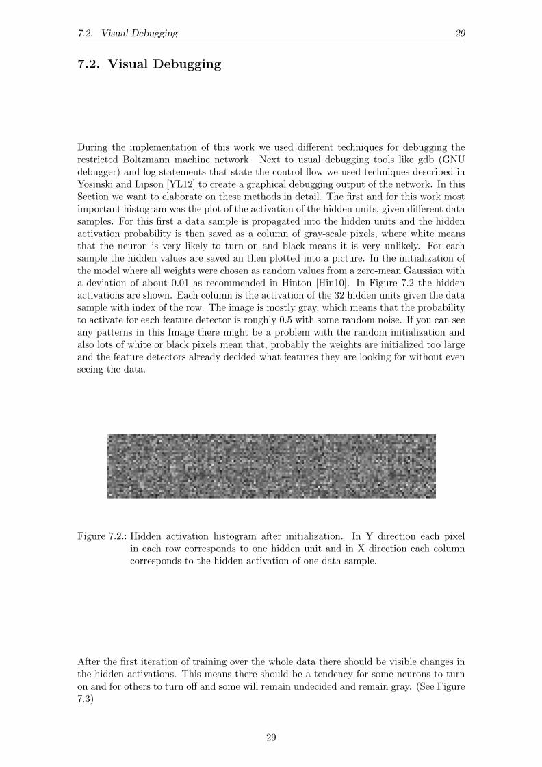
During the implementation of this work we used di↵erent techniques for debugging therestricted Boltzmann machine network. Next to usual debugging tools like gdb (GNUdebugger) and log statements that state the control flow we used techniques described inYosinski and Lipson [YL12] to create a graphical debugging output of the network. In thisSection we want to elaborate on these methods in detail. The first and for this work mostimportant histogram was the plot of the activation of the hidden units, given di↵erent datasamples. For this first a data sample is propagated into the hidden units and the hiddenactivation probability is then saved as a column of gray-scale pixels, where white meansthat the neuron is very likely to turn on and black means it is very unlikely. For eachsample the hidden values are saved an then plotted into a picture. In the initialization ofthe model where all weights were chosen as random values from a zero-mean Gaussian witha deviation of about 0.01 as recommended in Hinton [Hin10]. In Figure 7.2 the hiddenactivations are shown. Each column is the activation of the 32 hidden units given the datasample with index of the row. The image is mostly gray, which means that the probabilityto activate for each feature detector is roughly 0.5 with some random noise. If you can seeany patterns in this Image there might be a problem with the random initialization andalso lots of white or black pixels mean that, probably the weights are initialized too largeand the feature detectors already decided what features they are looking for without evenseeing the data.

Figure 7.2.: Hidden activation histogram after initialization. In Y direction each pixelin each row corresponds to one hidden unit and in X direction each columncorresponds to the hidden activation of one data sample.

After the first iteration of training over the whole data there should be visible changes inthe hidden activations. This means there should be a tendency for some neurons to turnon and for others to turn o↵ and some will remain undecided and remain gray. (See Figure7.3)

29

30 7. Implementation

Figure 7.3.: Hidden activation histogram after the first iteration of training. In Y directioneach pixel in each row corresponds to one hidden unit and in X direction eachcolumn corresponds to the hidden activation of one data sample.

If there are any patterns emerging it is possible that there is a bug in the implementation.The picture should mostly look like random noise and contain no visible forms. Onereason can be that the training data was not shu✏ed before training or not shu✏ed for thehistogram generation. Then depending on the task, in this example language modeling,some patterns can emerge at the boundaries between sentences. But with shu✏ed datathis histogram should mostly be random noise.

In Figure 7.4 there are lots of vertical visible patterns and also most of the neurons areturned on. In this graphic maybe the weights were initialized too big or this output mightbe normal for the task. For this it might be important to take a look at the second orthird iteration to see how the activations change.

Figure 7.4.: Vertical Patterns are visible.

In Figure 7.5 are some feature detectors that are highly likely to turn on for every datasample. This is a bad because these features will not help us classify anything since theyare always on anyway. This might point to a bug in the implementation and learning.

Figure 7.5.: Some units are on for all data samples.

Figure 7.6 is also an indicator of something not working right. We have a few data samplesfor which we get a repeating pattern and mostly gray in between. The pattern could be

30

7.2. Visual Debugging 31

explained by sentence endings but the gray area in between would mean that our modelcan classify some features at sentence ends but is totally indecisive elsewhere, which isalso unlikely. Since our data was shu✏ed, and the vertical visible patterns contain morethan one sample it is highly unlikely that the sentence ending n-grams stick together likethis. Maybe the random shu✏ing did not work correctly. Both the gray area and thepatter that is repeating over multiple samples more than one time are strong indicatorsthat there is a bug somewhere.

Figure 7.6.: The patterns that can be seen here look like there might be a bug. Dependingon the data patterns like this can happen but should not. Every columnrepresents a sample and the order of the samples were randomized so gettingequal looking patterns should not happen that often. Also the gray patternin between should not happen.

The last histogram we took a look at was the distribution of the visible and hidden biasesand weights. Normally the visible biases get initialized from the data. In our case themean value of the visible biases was 5.9. The hidden biases were initialized to zero andthe weights as explained above randomly from a Gaussian distribution with mean value 0and standard deviation of 0.1.

31

8. Evaluation

We evaluated the RBM-based language model on di↵erent statistical machine translation(SMT) tasks. We will first analyze what letter n-gram context is needed to be able todistinguish di↵erent words from the vocabulary well enough. Then we will give a briefdescription of our SMT system and afterwards, we will describe our experiments on theGerman-to-English TED and university lecture translation task in detail. After that wewill describe the results of the English-to-German news translation system and the English-to-French TED task. We will conclude this chapter with a brief discussion about the size ofthe newly proposed models and their training time. Since we did most of the experimentson the German-to-English TED task a complete table showing all results for each of thethree systems can be found in the Appendix A.

8.1. Word Representation

In first experiments we analyzed whether the letter-based representation is able to distin-guish between di↵erent words. In a vocabulary of 27,748 words, we compared for di↵erentletter n-gram sizes how many words are mapped to the same input feature vector.

#Vectors mapping toModel Caps VocSize #Vectors 1 Word 2 Words 3 Words 4+ Words

WordIndex - 27,748 27,748 27,748 0 0 0Letter 1-gram No 107 21,216 17,319 2,559 732 606Letter 2-gram No 1,879 27,671 27,620 33 10 8Letter 3-gram No 12,139 27,720 27,701 10 9 0Letter 3-gram Yes 8,675 27,710 27,681 20 9 0Letter 4-gram No 43,903 27,737 27,727 9 1 0Letter 4-gram Yes 25,942 27,728 27,709 18 1 0

Table 8.1.: Comparison of the vocabulary size and the possibility to have a unique repre-sentation of each word in the training corpus.

Table 8.1 shows the di↵erent models, their input dimensions and the total number ofunique clusters as well as the amount of input vectors containing one, two, three or four ormore words that get mapped to this input vector. In the word index representation everyword has its own feature vector. In this case the dimension of the input vector is 27,748and each word has its own unique input vector.

33

34 8. Evaluation

If we use only letters, as done in the unigram model, only 62% of the words have a uniquerepresentation. Furthermore, there are 606 feature vectors representing 4 or more words.This type of encoding of the words is not su�cient for the task.

When using a bigram letter context nearly each of the 27,748 words has a unique inputrepresentation, although the input dimension is only 7% compared to the word index. Withthe three letter vocabulary context and higher there is no input vector that represents morethan three words from the vocabulary. This is good since we want similar words to be closetogether but not have exactly the same input vector. The words that are still clustered tothe same input are mostly numbers or in case of the capital letter encoding typing mistakeslike “YouTube” and “Youtube”.

8.2. Translation System Description

The translation system for the German-to-English task was trained on the European Par-liament corpus, News Commentary corpus, the BTEC corpus and TED talks1. The datawas preprocessed and compound splitting was applied for German. Afterwards the dis-criminative word alignment approach as described in Niehues and Vogel [NV08] was ap-plied to generate the alignments between source and target words. The phrase table wasbuilt using the scripts from the Moses package described in Koehn et al. [KHB+07]. A4-gram language model was trained on the target side of the parallel data using the SRILMtoolkit from Stolcke [Sto02]. In addition, we used a bilingual language model as describedin Niehues et al. [NHVW11]. Reordering was performed as a preprocessing step usingpart-of-speech (POS) information generated by the TreeTagger [Sch94b]. We used thereordering approach described in Rottmann and Vogel [RV07] and the extensions pre-sented in Niehues et al. [NK09] to cover long-range reorderings, which are typical whentranslating between German and English. An in-house phrase-based decoder was used togenerate the translation hypotheses and the optimization was performed using the MERTimplementation as presented in Venugopal et al. [VZW05]. All our evaluation scores aremeasured using the BLEU metric.

We trained the RBMLM models on 50K sentences from TED talks and optimized theweights of the log-linear model on a separate set of TED talks. For all experiments theRBMLMs have been trained with a context of four words. The development set consistsof 1.7K segments containing 16K words. We used two di↵erent test sets to evaluate ourmodels. The first test set contains TED talks with 3.5K segments containing 31K words.The second task was from an in-house computer science lecture (CSL) corpus containing2.1K segments and 47K words. For both tasks we used the weights optimized on the TEDdata.

For the task of translating English news texts into German we used a system developed forthe Workshop on Machine Translation (WMT) evaluation. The continuous space languagemodels were trained on a random subsample of 100K sentences from the monolingualtraining data used for this task. The out-of-vocabulary rates for the TED task are 1.06%while the computer science lectures have 2.73% and nearly 1% on WMT.

1http://www.ted.com

34

8.3. German-to-English TED Task 35

8.3. German-to-English TED Task

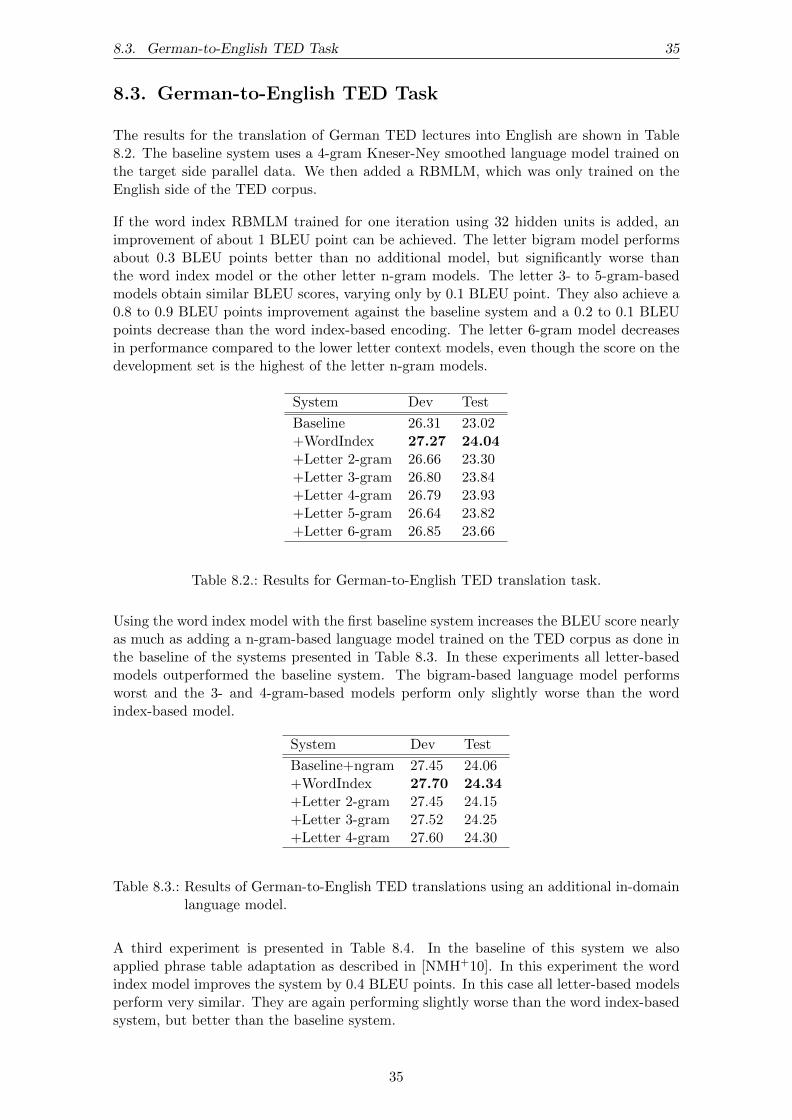
The results for the translation of German TED lectures into English are shown in Table8.2. The baseline system uses a 4-gram Kneser-Ney smoothed language model trained onthe target side parallel data. We then added a RBMLM, which was only trained on theEnglish side of the TED corpus.

If the word index RBMLM trained for one iteration using 32 hidden units is added, animprovement of about 1 BLEU point can be achieved. The letter bigram model performsabout 0.3 BLEU points better than no additional model, but significantly worse thanthe word index model or the other letter n-gram models. The letter 3- to 5-gram-basedmodels obtain similar BLEU scores, varying only by 0.1 BLEU point. They also achieve a0.8 to 0.9 BLEU points improvement against the baseline system and a 0.2 to 0.1 BLEUpoints decrease than the word index-based encoding. The letter 6-gram model decreasesin performance compared to the lower letter context models, even though the score on thedevelopment set is the highest of the letter n-gram models.

System Dev Test

Baseline 26.31 23.02+WordIndex 27.27 24.04+Letter 2-gram 26.66 23.30+Letter 3-gram 26.80 23.84+Letter 4-gram 26.79 23.93+Letter 5-gram 26.64 23.82+Letter 6-gram 26.85 23.66

Table 8.2.: Results for German-to-English TED translation task.

Using the word index model with the first baseline system increases the BLEU score nearlyas much as adding a n-gram-based language model trained on the TED corpus as done inthe baseline of the systems presented in Table 8.3. In these experiments all letter-basedmodels outperformed the baseline system. The bigram-based language model performsworst and the 3- and 4-gram-based models perform only slightly worse than the wordindex-based model.

System Dev Test

Baseline+ngram 27.45 24.06+WordIndex 27.70 24.34+Letter 2-gram 27.45 24.15+Letter 3-gram 27.52 24.25+Letter 4-gram 27.60 24.30

Table 8.3.: Results of German-to-English TED translations using an additional in-domainlanguage model.

A third experiment is presented in Table 8.4. In the baseline of this system we alsoapplied phrase table adaptation as described in [NMH+10]. In this experiment the wordindex model improves the system by 0.4 BLEU points. In this case all letter-based modelsperform very similar. They are again performing slightly worse than the word index-basedsystem, but better than the baseline system.

35

36 8. Evaluation

System Dev Test

Baseline+ngram+adaptpt 28.40 24.57+WordIndex 28.55 24.96+Letter 2-gram 28.31 24.80+Letter 3-gram 28.31 24.71+Letter 4-gram 28.46 24.65

Table 8.4.: Results of German-to-English TED translations with additional in-domain lan-guage model and adapted phrase table.

To summarize the results, we could always improve the performance of the baseline systemby adding the letter n-gram-based language model. Furthermore, in most cases, the bigrammodel performs worse than the higher order models. It seems to be important for thistask to have more context information. The 3- and 4-gram-based models perform almostequal, but slightly worse than the word index-based model.

8.3.1. Caps Feature

In this subsection we evaluate the proposed caps feature compared to the non-caps lettern-gram model and the baseline systems. For the sake of clarity the tables this time containthe results of one letter n-gram context on all three system configurations.

In Table 8.5 the scores for the baselines, the letter bigram models and the caps features canbe seen. It is notable that the capital letter variant improves the normal version except forthe last system. On the first system the letter bigram using caps features is still around0.3 BLEU points worse than the higher context letter n-gram models.

System Dev Test

Baseline 26.31 23.02+Letter 2-gram 26.66 23.30+Letter 2-gram caps 26.67 23.44

Baseline+ngram 27.45 24.06+Letter 2-gram 27.45 24.15+Letter 2-gram caps 27.46 24.28

Baseline+ngram+adaptpt 28.40 24.57+Letter 2-gram 28.31 24.80+Letter 2-gram caps 28.33 24.72

Table 8.5.: Di↵erence between caps and non-caps letter n-gram models.

As we can see in Table 8.6 the caps features with the letter 3-gram model improve thebaseline BLEU score by about ±0.2 BLEU points. As we saw in the case of the letterbigrams the 3-gram caps feature models perform slightly better than the normal versionwith the exception for the last task.

36

8.3. German-to-English TED Task 37

System Dev Test

Baseline 26.31 23.02+Letter 3-gram 26.80 23.84+Letter 3-gram caps 26.67 23.85

Baseline+ngram 27.45 24.06+Letter 3-gram 27.52 24.25+Letter 3-gram caps 27.60 24.47

Baseline+ngram+adaptpt 28.40 24.57+Letter 3-gram 28.31 24.71+Letter 3-gram caps 28.43 24.66

Table 8.6.: Di↵erence between caps and non-caps letter n-gram models.

In Table 8.7 we can see the results for the letter 4-gram models. In this case the capsfeatures only improve the last two systems. In the second system with the additionalin-domain language model the letter 4-gram caps model improves the baseline by about0.5 BLEU points which is even more than the word index model.

System Dev Test

Baseline 26.31 23.02+Letter 4-gram 26.79 23.93+Letter 4-gram caps 26.73 23.77Baseline+ngram 27.45 24.06+Letter 4-gram 27.60 24.30+Letter 4-gram caps 27.60 24.57

Baseline+ngram+adaptpt 28.40 24.57+Letter 4-gram 28.46 24.65+Letter 4-gram caps 28.43 24.73

Table 8.7.: Di↵erence between caps and non-caps letter n-gram models.

Concluding this subsection the caps features tend to improve the non-caps layers on theTED task. The improvement is on average around 0.08 BLEU points while the bestsystem improves by 0.27 BLEU points. Even though the English language does not containmany capital letter words the capital letter manages to improve the input layer while alsodecreasing the input size and thus reducing the training time.

37

38 8. Evaluation

8.3.2. Tree-Split Feature

In this subsection we are going to evaluate the tree split features. We concluded experi-ments with a tree depth of one and two using both capital letter features and just lettern-gram features and di↵erent letter n-gram sizes. The results for the first baseline systemcan be seen in Table 8.8. We can see that the tree split features decrease the performanceof the regular letter n-gram system on average by 0.2 BLEU points but still improve thebaseline without RBMLM by about 0.65 BLEU points.

System Dev Test

Baseline 26.31 23.02+Letter 3-gram 26.80 23.84+Letter 3-gram 1-TreeDepth 26.47 23.65+Letter 3-gram 2-TreeDepth 26.71 23.72+Letter 4-gram 26.79 23.93+Letter 4-gram 1-TreeDepth 26.79 23.67+Letter 4-gram 2-TreeDepth 26.74 23.73

Table 8.8.: The results of the tree split features for the TED baseline system.

As we can see in Table 8.9 the results for the system with the additional in-domain languagemodel show that depending on the system the tree split features can give an improvementover the conventional letter n-gram features. The performance of the tree split featurevaries from minus 0.03 BLEU points to plus 0.1 BLEU points compared to the lettern-gram input layer baseline. Still all tree split systems increase the BLEU score of thebaseline without continuous space language model.

System Dev Test

Baseline+ngram 27.45 24.06+Letter 3-gram 27.52 24.25+Letter 3-gram 1-TreeDepth 27.49 24.32+Letter 3-gram 2-TreeDepth 27.38 24.22+Letter 4-gram 27.60 24.30+Letter 4-gram 1-TreeDepth 27.66 24.27+Letter 4-gram 2-TreeDepth 27.63 24.33

Table 8.9.: The results of the tree split features for the TED system with additional in-domain language model.

In Table 8.10 for the third baseline system we can see that the tree split feature improvesthe letter 3-gram model. The best system, which is the letter 3-gram with tree depthof two improves over the normal input layer by 0.27 BLEU points, the same tree depthfor the letter 4-gram decreases the score by 0.2 which is even below the normal systembaseline.

38

8.3. German-to-English TED Task 39

System Dev Test

Baseline+ngram+adaptpt 28.40 24.57+Letter 3-gram 28.31 24.71+Letter 3-gram 1-TreeDepth 28.33 24.60+Letter 3-gram 2-TreeDepth 28.33 24.98

+Letter 4-gram 28.46 24.65+Letter 4-gram 1-TreeDepth 28.48 24.65+Letter 4-gram 2-TreeDepth 28.38 24.47

Table 8.10.: The results of the tree split features for the TED system with additional in-domain language model and adapted phrase table.

After seeing the first experiments on the three baseline systems we conclude that exceptfor the second TED system with the additional in-domain language model, the tree splitfeature does not work as well as the normal letter n-grams. This changes when we combinethe tree split and capital letter feature as can be seen in Table 8.11. We can see that usingthe tree depth one as additional feature increases the BLEU score by about 0.05 BLEUpoints while using a tree depth of two performs around 0.2 BLEU points worse.

System Dev Test

Baseline 26.31 23.02+Letter 3-gram caps 26.67 23.85+Letter 3-gram caps 1-TreeDepth 26.66 23.89+Letter 3-gram caps 2-TreeDepth 26.69 23.72+Letter 4-gram caps 26.73 23.77+Letter 4-gram caps 1-TreeDepth 26.79 23.81+Letter 4-gram caps 2-TreeDepth 26.60 23.54

Table 8.11.: The results of the tree split and caps features for the TED system.

The results for the system with the additional in-domain language model can be seen inTable 8.12. In this system configuration the tree split models all perform worse than thenewly proposed input layer without the tree split feature. The decrease for the letter 3-gram is about 0.07 BLEU points while the BLEU score of the letter 4-gram model decreasesby about 0.25 BLEU points.

System Dev Test

Baseline+ngram 27.45 24.06+Letter 3-gram caps 27.60 24.47+Letter 3-gram caps 1-TreeDepth 27.50 24.40+Letter 3-gram caps 2-TreeDepth 27.54 24.40+Letter 4-gram caps 27.46 24.57+Letter 4-gram caps 1-TreeDepth 27.60 24.37+Letter 4-gram caps 2-TreeDepth 27.50 24.23

Table 8.12.: The results of the tree split and caps features for the TED system with addi-tional in-domain language model.

The results for last configuration for the German-to-English TED task with additionalin-domain language model and additional phrase table can be seen in Table 8.13. Most of

39

40 8. Evaluation

the configurations are able to improve over the normal letter n-gram model. The averageincrease is about 0.05 BLEU points with the biggest increase being 0.12 BLEU points.

System Dev Test

Baseline+ngram+adaptpt 28.40 24.57+Letter 3-gram caps 28.43 24.66+Letter 3-gram caps 1-TreeDepth 28.37 24.61+Letter 3-gram caps 2-TreeDepth 28.26 24.77

+Letter 4-gram caps 28.38 24.73+Letter 4-gram caps 1-TreeDepth 28.35 24.85+Letter 4-gram caps 2-TreeDepth 28.39 24.75

Table 8.13.: The results of the tree split and caps features for the TED system with addi-tional in-domain language model and adapted phrase table.

Concluding this section, we found that all tree split except for one configuration improvethe score of the baseline. In the sorted tables in Appendix A we can see that except for thefirst TED baseline system tree split systems on average perform better than the normalletter n-gram input layer and that combining capital letter features combined with treesplit feature performs better on average than just using tree split features alone.

8.3.3. Iterations

As showed in Niehues andWaibel [NW12] training the RBMLM for more than one iterationmight be useful. We trained one of our letter n-gram models for 10 iterations and took the10th iteration for translation. In Table 8.14 we show the free energy for all the iterations.We can see that the free energy decreases between all iterations. After the first iterationthe average free energy of the training set is -9.27141 while after the 10th iteration itdecreased to -41.2808. On a held out development set the energy went down from -15.6257to -48.1398 being lowest in the 10th iteration.

Free EnergyIteration Dev Train

1 -15.6257 -9.271412 -30.4127 -23.68743 -32.7115 -25.84864 -30.5272 -23.75075 -45.7468 -38.79816 -45.5386 -39.32847 -46.8414 -38.43258 -48.0029 -40.06119 -48.1398 -41.031510 -48.1398 -41.2808

Table 8.14.: Changes of free energy during multiple iterations of training.

A low free energy in a restricted Boltzmann machine means a high probability, so the10th iteration should be the best trained model for our task. The results can be seen inTable 8.15, where it performed as well as trained for one Iteration. There was an increase

40

8.3. German-to-English TED Task 41

in performance for the word-index model, we could not find the letter n-gram model toimprove on the TED task by training multiple iterations.

System Dev Test

Baseline 26.31 23.02+WordIndex 1 Iter 27.27 24.04+WordIndex 10 Iter 27.61 24.47+Letter 3-gram 1 Iter 26.80 23.84+Letter 3-gram 10 Iter 26.76 23.85

Table 8.15.: The results for multiple iteration training on German-to-English TED task.

Concluding this section, we could not find the same improvement, as for the word indexmodel, training for multiple iterations using our newly proposed input layer. Since thefree energy of the training and development set decreased during training we can concludethat the model trained for more iterations models the data better than the model trainedfor only one Iteration. Not seeing an increase in BLEU score can have di↵erent reasonsand more experiments of di↵erent Systems would have to be done.

8.3.4. Hidden Size

In this subsection we want to present the results of the models having more than 32hidden units. We concluded the experiment on the first of the three German-to-EnglishTED systems and the results can be seen in Table 8.16. We chose to compare the 32hidden unit model with 64 and 128 hidden units.

System Dev Test

Baseline 26.31 23.02+WordIndex 32H 27.27 24.04+Letter 3-gram 32H 26.80 23.84+Letter 3-gram 64H 26.95 23.82+Letter 3-gram 128H 26.83 23.85

Table 8.16.: Results for German-to-English TED translation task.

The results show that increasing the hidden size did not increase the BLEU score on thetest set, while with 64 hidden units a small gain could be seen on the development data.

8.3.5. Combination of Models

Another experiment concerning the combination of models was done. We wanted to seeif the combination of the word index model, which performs well as a general languagemodel and the letter n-gram model, which tries improve on out-of-vocabulary words andmorphological word forms, could achieve better results.

For this we tried using both of the models as a log-linear feature in the decoder and alsotrained a new model containing both input layers. The results of this can be seen in Table8.17. The jointly trained models decrease the performance of the separate models slightly.It maybe that the joint training of the models could benefit from an additional trainingiteration or a larger hidden size. The log linear combinations of both models on the otherhand improved over the word index by 0.11 BLEU points. Concluding this subsection wefound that the combination of models can improve the gain in BLEU score even furtherthan using each model on its own.

41

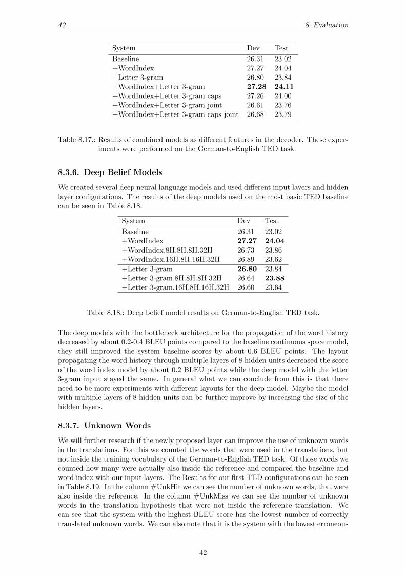
42 8. Evaluation

System Dev Test

Baseline 26.31 23.02+WordIndex 27.27 24.04+Letter 3-gram 26.80 23.84+WordIndex+Letter 3-gram 27.28 24.11+WordIndex+Letter 3-gram caps 27.26 24.00+WordIndex+Letter 3-gram joint 26.61 23.76+WordIndex+Letter 3-gram caps joint 26.68 23.79

Table 8.17.: Results of combined models as di↵erent features in the decoder. These exper-iments were performed on the German-to-English TED task.

8.3.6. Deep Belief Models

We created several deep neural language models and used di↵erent input layers and hiddenlayer configurations. The results of the deep models used on the most basic TED baselinecan be seen in Table 8.18.

System Dev Test

Baseline 26.31 23.02+WordIndex 27.27 24.04+WordIndex.8H.8H.8H.32H 26.73 23.86+WordIndex.16H.8H.16H.32H 26.89 23.62+Letter 3-gram 26.80 23.84+Letter 3-gram.8H.8H.8H.32H 26.64 23.88+Letter 3-gram.16H.8H.16H.32H 26.60 23.64

Table 8.18.: Deep belief model results on German-to-English TED task.

The deep models with the bottleneck architecture for the propagation of the word historydecreased by about 0.2-0.4 BLEU points compared to the baseline continuous space model,they still improved the system baseline scores by about 0.6 BLEU points. The layoutpropagating the word history through multiple layers of 8 hidden units decreased the scoreof the word index model by about 0.2 BLEU points while the deep model with the letter3-gram input stayed the same. In general what we can conclude from this is that thereneed to be more experiments with di↵erent layouts for the deep model. Maybe the modelwith multiple layers of 8 hidden units can be further improve by increasing the size of thehidden layers.

8.3.7. Unknown Words

We will further research if the newly proposed layer can improve the use of unknown wordsin the translations. For this we counted the words that were used in the translations, butnot inside the training vocabulary of the German-to-English TED task. Of those words wecounted how many were actually also inside the reference and compared the baseline andword index with our input layers. The Results for our first TED configurations can be seenin Table 8.19. In the column #UnkHit we can see the number of unknown words, that werealso inside the reference. In the column #UnkMiss we can see the number of unknownwords in the translation hypothesis that were not inside the reference translation. Wecan see that the system with the highest BLEU score has the lowest number of correctlytranslated unknown words. We can also note that it is the system with the lowest erroneous

42

8.3. German-to-English TED Task 43

translated unknown words. From this table it seems that the increase in BLEU scoredepends more on the decrease of wrong translated unknowns than the correct translationof unknown words.

System #UnkHit #UniqeHit #UnkMiss #UniqueMiss BLEU

Baseline 184 121 468 379 23.02WordIndex 177 115 420 345 24.04Letter 3-gram caps 183 119 457 365 23.85Letter 4-gram caps 182 118 452 367 23.77

Table 8.19.: Unknown words in hypothesis of the German-to-English TED system. Thetable shows both, correct use of an unknown word and the use of unknownwords that were not inside the reference.

In the second configuration seen in Table 8.20 we can see that the unknowns that are insidethe translations and the reference is again highest for the baseline. The wrong unknownwords are again lowest for the word index model being nearly 200 less than the baseline. Inthis task even though the BLEU score increased the number of mistaken unknown wordsalso increased overall and is lowest for the word-index model.

System #UnkHit #UniqeHit #UnkMiss #UniqueMiss BLEU

Baseline+ngram 189 126 643 529 24.06WordIndex 180 118 446 368 24.34Letter 3-gram caps 186 123 539 439 24.47Letter 4-gram caps 183 120 508 421 24.57

Table 8.20.: Unknown words in hypothesis of the German-to-English TED system withadditional in-domain language model. The table shows both, correct use ofan unknown word and mistranslations.

In Table 8.21 we can see the results for the configuration with additional language modeland adapted phrase table. The number of unknown words used in the translation andreference is almost equal for all systems, while the number of wrong unknowns used islowest for the letter 4-gram model using caps features.

System #UnkHit #UniqeHit #UnkMiss #UniqueMiss BLEU

Baseline+ngram+adaptpt 180 118 435 370 24.57WordIndex 180 118 428 373 24.96Letter 3-gram caps 179 117 419 357 24.66Letter 4-gram caps 180 118 414 353 24.73

Table 8.21.: Unknown words in hypothesis of the German-to-English TED system withadditional in-domain language model and adapted phrase table. The tableshows both, correct use of an unknown word and mistranslations.

In Table 8.22 the total number of unknown words and words in the reference is listed.From a total of 3719 unique words in the reference we have 372 ( 10 %) unknown wordsthat are not inside the vocabulary of the RBMLM. Out of these 372 words about 120( 32%) were translated correctly in every configuration.

43

44 8. Evaluation

ReferenceTotal Unk 506Unique Unk 372Total Words 32184Unique Words 3719

Table 8.22.: Number of Tokens not inside vocabulary

Concluding this section we can say that on TED there was no obvious connection betweenthe number of correct and incorrect used unknown words. In the first configurations thesystem with the best BLEU score had the least incorrect used unknown words, while inthe second configuration the best system had neither the most correct used nor the leastincorrect used unknown words. On average the letter n-gram layer more correct unknownwords than the word index input layer, but also uses more incorrect unknown words.

8.4. German-to-English CSL Task

After that, we evaluated the computer science lecture (CSL) test set. We used the samesystem as for the TED translation task. We did not perform a new optimization, since wewanted so see how well the models performed on a di↵erent task.

The results are summarized in Table 8.23. In this case the baseline is outperformed by theword index approach by approximately 1.1 BLEU points. Except for the 4-gram modelthe results are similar to the result for the TED task. All systems could again outperformthe baseline.

System Test

Baseline 23.60+WordIndex 24.76+Letter 2-gram 24.17+Letter 3-gram 24.36+Letter 4-gram 23.82

Table 8.23.: Results the baseline of the German-to-English CSL task.

The system with the additional in-domain language model in Table 8.24 shows that bothletter n-gram language models perform better than the baseline and the word index model,improving the baseline by about 0.8 to 1 BLEU points. Whereas the word index modelonly achieved an improvement of 0.6 BLEU points.

System Test

Baseline+ngram 23.81+WordIndex 24.41+Letter 2-gram 24.37+Letter 3-gram 24.66+Letter 4-gram 24.85

Table 8.24.: Results on German-to-English CSL corpus with additional in-domain languagemodel.

44

8.5. English-to-German News Task 45

The results of the system with the additional phrase table adaption can be seen in Table8.25. The word index model improves the baseline by 0.25 BLEU points. The letter n-gram models improve the baseline by about 0.3 to 0.4 BLEU points also improving overthe word index model. The letter bigram model in this case performs worse than thebaseline.

System Test

BL+ngram+adaptpt 25.00+WordIndex 25.25+Letter 2-gram 24.68+Letter 3-gram 25.43+Letter 4-gram 25.33

Table 8.25.: Results on German-to-English CSL with additional in-domain language modeland adapted phrase table.

In summary, again the 3- and 4-gram letter models perform mostly better than the bigramversion. They both almost equal. In contrast to the TED task, they were even able tooutperform the word index model in some configurations by up to 0.4 BLEU points.

8.5. English-to-German News Task

The English-to-German news task was released for the Workshop on Statistical MachineTranslation (WMT) 2013 conference. It consists of English-to-German news translations.We expect our input encoding to work better on this task since German has more wordmorphologies than the English language. The system presented in Table 8.26 uses discrim-inative word alignment, a bilingual language model, and a class-based language model aswell as a discriminative word lexicon. With this system we could not improve the per-formance of the baseline by using a word index model, but in contrast the performancedropped by 0.1 BLEU points. If we use a letter bigram model, we could improve thetranslation quality by 0.1 BLEU points over the baseline system.

System Dev Test

Baseline 16.90 17.36+WordIndex 16.79 17.29+Letter 2-gram 16.91 17.48

Table 8.26.: Results for WMT2013 task English-to-German news.

The system presented in Table 8.27 has an additional POS-based language model and useslexicalized reordering rules as well as tree rules for reordering. The letter bigram model isable to improve over the baseline by about 0.14 BLEU points.

System Dev Test

Baseline 17.21 17.59+Letter 2-gram 16.91 17.73

Table 8.27.: Results for WMT2013 task English-to-German news.

Concluding this section we were able to improve the baseline on a English-to-German task.In this task, similar to the CSL lectures the word-index RBMLM failed to improve the

45

46 8. Evaluation

baseline while the letter n-gram model showed to give an increase of about 0.1 BLEUpoints. Further experiments with higher letter n-gram context have to be concluded tosee if the BLEU score can be increased even further.

8.6. English-to-French TED Task

In this section we are going to evaluate the English-to-French translation task. In Table8.28 we can see that the RBMLMs, except for the letter 2-gram model, provide only avery small increase in BLEU score. The best model is the letter 3-gram with capital letterfeature increasing BLEU by about 0.07 points.

System Dev Test

Baseline 29.15 32.13+WordIndex 29.17 32.18+Letter 2-gram 29.17 31.92+Letter 2-gram caps 29.21 31.89+Letter 3-gram 29.25 31.92+Letter 3-gram caps 28.98 32.20

Table 8.28.: Results for English-to-French TED translation task

Concluding this section we found that the French baseline could only be improved by theWordIndex and letter 3-gram model using caps features. It is interesting to note that eventhough the letter 3-gram caps model performed worse on the development data than anyother system, it achieved the best BLEU score on the test data.

8.7. Model Size and Training Times

In general the letter n-gram models perform almost as good as the word index model onEnglish language tasks. The advantage of the models up to the letter 3-gram context modelis that the training time is lower compared to the word index model. All the models weretrained using 10 cores and a batch size of 10 samples per Contrastive Divergence update.As can be seen in Table 8.29 the letter 3-gram model needs less than 50% of the weightsand takes around 75% of the training time of the word index model. The four letter n-grammodel takes longer to train due to more parameters.

Even though the letter 5-gram model has 12.5 million parameters the performance wasnot as good as the lower context models. With this many parameters it is harder to findgood values for the weights, which means that more training could prove to improve theperformance. We can also see that the letter 2-gram model is very small and easy totrain. This might be good for big systems like we saw in the English-to-German WMTtask where the letter 2-gram model even improved over the word index model. The deepbelief networks took less than half of the time the corresponding basic model needed. Thisshows great potential since the performance of the deep letter 3-gram models was nearlyas good as the normal letter 3-gram model.

46

8.7. Model Size and Training Times 47

Model #Weights Time

WordIndex 3.55 M 20 h 10 minLetter 2-gram 0.24 M 1h 24 minLetter 3-gram 1.55 M 15 h 12 minLetter 3-gram caps 1.11 M 10 h 32 minLetter 3-gram 1-TreeDepth 3.3 M 20 h 11 minLetter 3-gram caps 1-TreeDepth 2.5 M 18 h 43 minLetter 3-gram 2-TreeDepth 4.9 M 27 h 34 minLetter 3-gram caps 2-TreeDepth 3.7 M 24 h 07 minLetter 4-gram 5.62 M 38 h 59 minLetter 5-gram 12.53 M 63 h 01 minLetter 3-gram.8H.8H.8H.32H 0.68 M 6 h 18 minLetter 3-gram.16H.8H.16H.32H 0.97 M 8 h 04 min

Table 8.29.: Training time and number of parameters of the RBMLM models.

47

9. Future Work & Conclusion

In this work we developed new input encoding features for continuous space languagemodels. The so called letter n-gram approach uses sub-word letter n-grams to representwords and help to still evaluate words that were never seen in the vocabulary. We thinkthat this input layer helps to learn di↵erent morphological features inside the hiddenrepresentation of the network. We also found that it is useful to add additional featuredetectors that represent whether the word is written in capital letters or even all capitalletters, e.g. abbreviations. The last feature we tried was the Tree-Split algorithm. Wewanted to see if it is helpful to store more data about the position of the letter n-graminside the word. For this we split the word in half creating a tree structure where in eachdepth the letter n-grams get additional information appended. We did several experimentsto explore if the newly proposed input layers can achieve an improvement over commonapproach input layouts. We evaluated if the input layer is able to classify unknown wordsbetter and give more accurate probabilities for word n-grams. We compared them usingmultiple languages and di↵erent translation systems. For this we used lecture translationtasks using the TED dataset and the in-house computer science lecture corpus and ona system used for the WMT 2013 conference. The languages used were French, Englishand German. In every setup the normal letter n-gram approach was able to improvethe baseline and depending on the task even outperform the word index model. If we useadditional features like capital letter information or the tree split feature we were sometimesable to outperform the word index model and normal letter n-gram models. The capitalletter feature reduced the parameters to train even more while generalizing over a biggerword space. On average the capital letter feature helped to improve the normal lettern-gram layer even on a language like English, where only few capitalized words are used.For the tree split feature we saved the order in which the letter n-grams appeared in a treestructure to see if the information that certain letter n-grams are more probable at theend of the word than in the beginning is useful. This feature on the contrary increasedthe input size of the model while in one case even decreasing the performance comparedto the baseline. In general the performance of the tree split models were good while webelieve that a tree depth of one and additional capital letter feature achieved the bestperformance of all tree split feature systems on average.

We believe the optimal n-gram context to be three for the English language and instead ofincreasing the letter n-gram context rather increase the hidden size and training iterations.Even though the experiments showed that on the German-to-English TED task trainingfor 10 iterations did not increase the BLEU score, the free energy of test and development

49

50 9. Future Work & Conclusion

data decreased, which means that the average probability of those sentences increased.

Another advantage of the subword feature layer is, that the input layer size and hencethe training time and number of parameters is reduced a decrease to 75 % of the trainingtime can be achieved. In some cases a bigram letter model achieved better scores than thecommon word index approach using only a tenth of the training time.

The second part of this work researched a layout for a deep belief network to classify n-grams. In the initial experiments we found that the performance compared to the shallowarchitecture using the same input layer decreased on average. But this might be due to thefact that the deep models we trained had far less parameters than the shallow architectures.The problem with bigger networks was that the evaluation time of the n-gram probabilitieswhile decoding took very long. We believe that more experiments using bigger models hasto be done to make a qualified statement about the chosen architecture.

In the future more experiments of di↵erent systems and languages would have to be con-cluded to see if the models provide even more useful on languages like Arabic, where lotsof word morphologies are used. We would also like to do more experiments using the deeplayout and maybe even compare more deep layouts with each other. We also believe thatputting more e↵ort in joint training of di↵erent input layers might increase the gain inBLEU points. Porting the learning algorithm onto a GPU could help to make the trainingof even bigger models or training more iterations feasible. Using additional features likepart-of-speech could help to further improve the letter n-gram models. The shallow RBMstructure in general might be useful to see if translation models can be learned. Thishas been done with feed forward neural networks [SAY12, Sch12], but not with shallowrestricted Boltzmann machine models.

50

Bibliography

[BDVJ03] Y. Bengio, R. Ducharme, P. Vincent, and C. Jauvin, “A Neural ProbabilisticLanguage Model,” Journal of Machine Learning Research, vol. 3, pp. 1137–1155, 2003.

[CG96] S. F. Chen and J. Goodman, “An empirical study of smoothing techniquesfor language modeling,” in Proceedings of the 34th annual meeting on Associ-ation for Computational Linguistics, ser. ACL ’96. Stroudsburg, PA, USA:Association for Computational Linguistics, 1996, pp. 310–318.

[CPH] M. A. Carreira-Perpinan and G. E. Hinton, “On Contrastive Divergence Learn-ing.”

[DYDA12] G. E. Dahl, D. Yu, L. Deng, and A. Acero, “Context-Dependent Pre-TrainedDeep Neural Networks for Large-Vocabulary Speech Recognition,” IEEETransactions on Audio, Speech & Language Processing, vol. 20, no. 1, pp.30–42, 2012.

[EZM08] A. Emami, I. Zitouni, and L. Mangu,“Rich morphology based n-gram languagemodels for Arabic,” in INTERSPEECH. ISCA, 2008, pp. 829–832.

[Gal91] S. I. Gallant,“A Practical Approach for Representing Context and for Perform-ing Word Sense Disambiguation Using Neural Networks,”Neural Computation,vol. 3, no. 3, pp. 293–309, 2013/03/14 1991.

[HDY+12] G. Hinton, L. Deng, D. Yu, G. Dahl, A. rahman Mohamed, N. Jaitly, A. Se-nior, V. Vanhoucke, P. Nguyen, T. Sainath, and B. Kingsbury, “Deep NeuralNetworks for Acoustic Modeling in Speech Recognition,” Signal ProcessingMagazine, 2012.

[Hin02] G. E. Hinton, “Training products of experts by minimizing contrastive diver-gence,”Neural Comput., vol. 14, no. 8, pp. 1771–1800, Aug. 2002.

[Hin10] G. Hinton, “A Practical Guide to Training Restricted Boltzmann Machines,”University of Toronto, Tech. Rep., 2010.

[HOT06] G. E. Hinton, S. Osindero, and Y.-W. Teh, “A fast learning algorithm for deepbelief nets,”Neural Comput., vol. 18, no. 7, pp. 1527–1554, July 2006.

[HS06] G. Hinton and R. Salakhutdinov, “Reducing the Dimensionality of Data withNeural Networks,” Science, vol. 313, no. 5786, pp. 504 – 507, 2006.

[Kat87] S. M. Katz, “Estimation of probabilities from sparse data for the languagemodel component of a speech recognizer,” in IEEE Transactions on Acoustics,Speech and Signal Processing, 1987, pp. 400–401.

[KHB+07] P. Koehn, H. Hoang, A. Birch, C. Callison-Burch, M. Federico, N. Bertoldi,B. Cowan, W. Shen, C. Moran, R. Zens, C. Dyer, O. Bojar, A. Constantin, andE. Herbst, “Moses: Open Source Toolkit for Statistical Machine Translation,”

51

52 Bibliography

in Proceedings of the 45th Annual Meeting of the ACL on Interactive Posterand Demonstration Sessions, ser. ACL ’07, Stroudsburg, PA, USA, 2007, pp.177–180.

[KN95] R. Kneser and H. Ney, “Improved backing-o↵ for n-gram language modeling,”in In Proceedings of the IEEE International Conference on Acoustics, Speechand Signal Processing, vol. I, Detroit, Michigan, May 1995, pp. 181–184.

[KY05] K. Kirchho↵ and M. Yang, “Improved Language Modeling for Statistical Ma-chine Translation,” in Proceedings of the ACL Workshop on Building and UsingParallel Texts, Ann Arbor, Michigan, USA, 2005, pp. 125–128.

[LOM+11] H. S. Le, I. Oparin, A. Messaoudi, A. Allauzen, J.-L. Gauvain, and F. Yvon,“Large Vocabulary SOUL Neural Network Language Models,” in INTER-SPEECH. ISCA, 2011, pp. 1469–1472.

[MD91] R. Miikkulainen and M. G. Dyer, “Natural Language Processing with ModularPDP Networks and Distributed Lexicon,”Cognitive Science, vol. 15, pp. 343–399, 1991.

[MH07] A. Mnih and G. Hinton, “Three new graphical models for statistical languagemodelling,” in Proceedings of the 24th International Conference on MachineLearning, 2007, pp. 641–648.

[MKB+10] T. Mikolov, M. Karafiat, L. Burget, J. Cernocky, and S. Khudanpur, “Recur-rent Neural Network Based Language Model,” in INTERSPEECH 2010, 11thAnnual Conference of the International Speech Communication Association,Makuhari, Chiba, Japan, 2010, pp. 1045–1048.

[Mni10] A. Mnih, “Learning Distributed Representations For Statistical LanguageModelling And Collaborative Filtering,” Ph.D. dissertation, University ofToronto, Toronto, Ont., Canada, Canada, 2010.

[Nea92] R. M. Neal, “Connectionist learning of belief networks,”Artif. Intell., vol. 56,no. 1, pp. 71–113, Jul. 1992.

[NHVW11] J. Niehues, T. Herrmann, S. Vogel, and A. Waibel, “Wider context by usingbilingual language models in machine translation,” in Proceedings of the SixthWorkshop on Statistical Machine Translation, ser. WMT ’11. Stroudsburg,PA, USA: Association for Computational Linguistics, 2011, pp. 198–206.

[NK09] J. Niehues and M. Kolss, “A POS-based model for long-range reorderings inSMT,” in Proceedings of the Fourth Workshop on Statistical Machine Transla-tion, ser. StatMT ’09. Stroudsburg, PA, USA: Association for ComputationalLinguistics, 2009, pp. 206–214.

[NMH+10] J. Niehues, M. Mediani, T. Herrmann, M. Heck, C. Her↵, and A. Waibel, “TheKIT Translation system for IWSLT 2010,” in Proceedings of the seventh Inter-national Workshop on Spoken Language Translation (IWSLT), Paris, France,2010.

[NMKS90] M. Nakamura, K. Maruyama, T. Kawabata, and K. Shikano, “Neural networkapproach to word category prediction for English texts,” in Proceedings of the13th conference on Computational linguistics - Volume 3, ser. COLING ’90,Stroudsburg, PA, USA, 1990, pp. 213–218.

[NV08] J. Niehues and S. Vogel, “Discriminative word alignment via alignment ma-trix modeling,” in Proceedings of the Third Workshop on Statistical MachineTranslation, ser. StatMT ’08, Stroudsburg, PA, USA, 2008, pp. 18–25.

52

Bibliography 53

[NW12] J. Niehues and A. Waibel, “Continuous Space Language Models using Re-stricted Boltzmann Machines,” in Proceedings of the International Workshopfor Spoken Language Translation (IWSLT 2012), Hong Kong, 2012.

[rMDH12] A. rahman Mohamed, G. E. Dahl, and G. E. Hinton, “Acoustic Modeling Us-ing Deep Belief Networks,” IEEE Transactions on Audio, Speech & LanguageProcessing, vol. 20, no. 1, pp. 14–22, 2012.

[RV07] K. Rottmann and S. Vogel, “Word Reordering in Statistical Machine Transla-tion with a POS-Based Distortion Model,” in TMI, Skovde, Sweden, 2007.

[SAY12] L. H. Son, A. Allauzen, and F. Yvon, “Continuous Space Translation ModelsWith Neural Networks,” in Proceedings of the 2012 Conference of the NorthAmerican Chapter of the Association for Computational Linguistics: HumanLanguage Technologies, ser. NAACL HLT ’12. Stroudsburg, PA, USA: Asso-ciation for Computational Linguistics, 2012, pp. 39–48.

[Sch94a] H. Schmid, “Part-Of-Speech Tagging With Neural Networks,” in Proceedingsof the 15th conference on Computational linguistics - Volume 1, ser. COLING’94. Stroudsburg, PA, USA: Association for Computational Linguistics, 1994,pp. 172–176.

[Sch94b] ——,“Probabilistic Part-of-Speech Tagging Using Decision Trees,” in Interna-tional Conference on New Methods in Language Processing, Manchester, UK,1994.

[Sch07] H. Schwenk, “Continuous Space Language Models,” Comput. Speech Lang.,vol. 21, no. 3, pp. 492–518, July 2007.

[Sch10] ——, “Continuous-Space Language Models for Statistical Machine Transla-tion,” Prague Bull. Math. Linguistics, vol. 93, pp. 137–146, 2010.

[Sch12] ——, “Continuous Space Translation Models for Phrase-Based Statistical Ma-chine Translation,” in COLING (Posters), M. Kay and C. Boitet, Eds. IndianInstitute of Technology Bombay, 2012, pp. 1071–1080.

[SD07] R. Sarikaya and Y. Deng, “Joint Morphological-Lexical Language Modelingfor Machine Translation,” in Human Language Technologies 2007: The Con-ference of the North American Chapter of the Association for ComputationalLinguistics; Companion Volume, Short Papers, Rochester, New York, USA,2007, pp. 145–148.

[SG05] H. Schwenk and J.-L. Gauvain, “Training Neural Network Language ModelsOn Very Large Corpora,” in Proceedings of the conference on Human LanguageTechnology and Empirical Methods in Natural Language Processing, ser. HLT’05. Stroudsburg, PA, USA: Association for Computational Linguistics, 2005,pp. 201–208.

[SMSN11] M. A. B. Shaik, A. E.-D. Mousa, R. Schluter, and H. Ney, “Hybrid LanguageModels Using Mixed Types of Sub-Lexical Units for Open Vocabulary Germanlvcsr,” in INTERSPEECH 2011, 12th Annual Conference of the InternationalSpeech Communication Association, Florence, Italy., 2011.

[SRA12] H. Schwenk, A. Rousseau, and M. Attik, “Large, Pruned or Continuous SpaceLanguage Models on a GPU for Statistical Machine Translation,” in NAACLWorkshop on the Future of Language Modeling, June 2012.

[SSG10] H. Sak, M. Saraclar, and T. Guengoer, “Morphology-based and Sub-word Lan-guage Modeling for Turkish Speech Recognition,” in 2010 IEEE International

53

54 Bibliography

Conference on Acoustics Speech and Signal Processing (ICASSP), 2010, pp.5402–5405.

[Sto02] A. Stolcke, “SRILM - An Extensible Language Modeling Toolkit,”in 7th International Conference on Spoken Language Processing, IC-SLP2002/INTERSPEECH 2002, Denver, Colorado, USA., 2002.

[VZW05] A. Venugopal, A. Zollmann, and A. Waibel, “Training and Evaluating ErrorMinimization Rules for Statistical Machine Translation,” in Proceedings ofthe ACL Workshop on Building and Using Parallel Texts, ser. ParaText ’05.Stroudsburg, PA, USA: Association for Computational Linguistics, 2005, pp.208–215.

[WHH+90] A. Waibel, T. Hanazawa, G. Hinton, K. Shikano, and K. J. Lang, “PhonemeRecognition using Time-delay Neural Networks,” in Readings in Speech Recog-nition, A. Waibel and K.-F. Lee, Eds. San Francisco, CA, USA: MorganKaufmann Publishers Inc., 1990, pp. 393–404.

[XR00] W. Xu and A. Rudnicky, “Can Artificial Neural Networks learn LanguageModels?” in Sixth International Conference on Spoken Language Processing,ICSLP 2000 / INTERSPEECH 2000, Beijing, China. ISCA, 2000, pp. 202–205.

[YL12] J. Yosinski and H. Lipson, “Visually Debugging Restricted Boltzmann Ma-chine Training with a 3D Example,” in Presented at Representation LearningWorkshop, 29th International Conference on Machine Learning, 2012.

54

Appendix

A. Complete Tables for each Task

In this section we want to show the complete tables for the German-to-English TED task.The first two tables show the basic baseline and the experiments done. The next two tablesshow the experiments for the task with the additional in-domain language model and thelast two tables show the experiments for the additional language model and adapted phrasetable. The first of each Table is sorted by experiments with the best scores marked as boldand the second tables are sorted by ascending BLEU scores.

System Dev Test

Baseline 26.31 23.02+WordIndex 27.27 24.04+WordIndex 10 Iter 27.61 24.47+WordIndex+Letter 3-gram 27.28 24.11+WordIndex+Letter 3-gram caps 27.26 24.00+WordIndex.8H.8H.8H.32H 26.73 23.86+WordIndex.16H.8H.16H.32H 26.89 23.62+Letter 2-gram 26.66 23.30+Letter 2-gram caps 26.67 23.44+Letter 3-gram 26.80 23.84+Letter 3-gram 10 Iter 26.76 23.85+Letter 3-gram.8H.8H.8H.32H 26.64 23.88+Letter 3-gram.16H.8H.16H.32H 26.60 23.64+Letter 3-gram caps 26.67 23.85+Letter 3-gram 1-TreeDepth 26.47 23.65+Letter 3-gram 2-TreeDepth 26.71 23.72+Letter 3-gram caps 1-TreeDepth 26.66 23.89+Letter 3-gram caps 2-TreeDepth 26.69 23.72+Letter 4-gram 26.79 23.93+Letter 4-gram caps 26.73 23.77+Letter 4-gram 1-TreeDepth 26.79 23.67+Letter 4-gram 2-TreeDepth 26.74 23.73+Letter 4-gram caps 1-TreeDepth 26.79 23.81+Letter 4-gram caps 2-TreeDepth 26.60 23.54+Letter 5-gram 26.64 23.82

Table A.1.: Results for German-to-English TED translation task for all experiments, sortedby task.

55

56 Appendix

System Dev Test

Baseline 26.31 23.02+Letter 2-gram 26.66 23.30+Letter 2-gram caps 26.67 23.44+Letter 4-gram caps 2-TreeDepth 26.60 23.54+WordIndex.16H.8H.16H.32H 26.89 23.62+Letter 3-gram.16H.8H.16H.32H 26.60 23.64+Letter 3-gram 1-TreeDepth 26.47 23.65+Letter 4-gram 1-TreeDepth 26.79 23.67+Letter 3-gram caps 2-TreeDepth 26.69 23.72+Letter 3-gram 2-TreeDepth 26.71 23.72+Letter 4-gram 2-TreeDepth 26.74 23.73+Letter 4-gram caps 26.73 23.77+Letter 4-gram caps 1-TreeDepth 26.79 23.81+Letter 5-gram 26.64 23.82+Letter 3-gram 26.80 23.84+Letter 3-gram caps 26.67 23.85+Letter 3-gram 10 Iter 26.76 23.85+WordIndex.8H.8H.8H.32H 26.73 23.86+Letter 3-gram.8H.8H.8H.32H 26.64 23.88+Letter 3-gram caps 1-TreeDepth 26.66 23.89+Letter 4-gram 26.79 23.93+WordIndex+Letter 3-gram caps 27.26 24.00+WordIndex 27.27 24.04+WordIndex+Letter 3-gram 27.28 24.11+WordIndex 10 Iter 27.61 24.47

Table A.2.: Results for German-to-English TED translation task for all experiments, sortedby ascending BLEU score .

56

A. Complete Tables for each Task 57

System Dev Test

Baseline+ngram 27.45 24.06+WordIndex 27.70 24.34+Letter 2-gram 27.45 24.15+Letter 2-gram caps 27.46 24.28+Letter 3-gram 27.52 24.25+Letter 3-gram caps 27.60 24.47+Letter 3-gram 1-TreeDepth 27.49 24.32+Letter 3-gram 2-TreeDepth 27.38 24.22+Letter 3-gram caps 1-TreeDepth 27.50 24.40+Letter 3-gram caps 2-TreeDepth 27.54 24.40+Letter 4-gram 27.60 24.30+Letter 4-gram caps 27.60 24.57+Letter 4-gram 1-TreeDepth 27.66 24.27+Letter 4-gram 2-TreeDepth 27.63 24.33+Letter 4-gram caps 1-TreeDepth 27.60 24.37+Letter 4-gram caps 2-TreeDepth 27.50 24.23

Table A.3.: Results for German-to-English TED translation task using an additional in-domain language model for all experiments, sorted by task.

System Dev Test

Baseline+ngram 27.45 24.06+Letter 2-gram 27.45 24.15+Letter 3-gram 2-TreeDepth 27.38 24.22+Letter 4-gram caps 2-TreeDepth 27.50 24.23+Letter 3-gram 27.52 24.25+Letter 4-gram 1-TreeDepth 27.66 24.27+Letter 2-gram caps 27.46 24.28+Letter 4-gram 27.60 24.30+Letter 3-gram 1-TreeDepth 27.49 24.32+Letter 4-gram 2-TreeDepth 27.63 24.33+WordIndex 27.70 24.34+Letter 4-gram caps 1-TreeDepth 27.60 24.37+Letter 3-gram caps 1-TreeDepth 27.50 24.40+Letter 3-gram caps 2-TreeDepth 27.54 24.40+Letter 3-gram caps 27.60 24.47+Letter 4-gram caps 27.60 24.57

Table A.4.: Results for German-to-English TED translation task using an additional in-domain language model for all experiments, sorted by ascending BLEU scores.

57

58 Appendix

System Dev Test

Baseline+ngram+adaptpt 28.40 24.57+WordIndex 28.55 24.96+Letter 2-gram 28.31 24.80+Letter 2-gram caps 28.33 24.72+Letter 3-gram 28.31 24.71+Letter 3-gram caps 28.43 24.66+Letter 3-gram 1-TreeDepth 28.33 24.60+Letter 3-gram 2-TreeDepth 28.33 24.98+Letter 3-gram caps 1-TreeDepth 28.37 24.61+Letter 3-gram caps 2-TreeDepth 28.26 24.77+Letter 4-gram 28.46 24.65+Letter 4-gram caps 28.43 24.73+Letter 4-gram 1-TreeDepth 28.48 24.65+Letter 4-gram 2-TreeDepth 28.38 24.47+Letter 4-gram caps 1-TreeDepth 28.35 24.85+Letter 4-gram caps 2-TreeDepth 28.39 24.75

Table A.5.: Results for German-to-English TED translation task using an additional in-domain language model for all experiments, sorted by task.

System Dev Test

+Letter 4-gram 2-TreeDepth 28.38 24.47Baseline+ngram+adaptpt 28.40 24.57+Letter 3-gram 1-TreeDepth 28.33 24.60+Letter 3-gram caps 1-TreeDepth 28.37 24.61+Letter 4-gram 28.46 24.65+Letter 4-gram 1-TreeDepth 28.48 24.65+Letter 3-gram caps 28.43 24.66+Letter 3-gram 28.31 24.71+Letter 2-gram caps 28.33 24.72+Letter 4-gram caps 28.43 24.73+Letter 4-gram caps 2-TreeDepth 28.39 24.75+Letter 3-gram caps 2-TreeDepth 28.26 24.77+Letter 2-gram 28.31 24.80+Letter 4-gram caps 1-TreeDepth 28.35 24.85+WordIndex 28.55 24.96+Letter 3-gram 2-TreeDepth 28.33 24.98

Table A.6.: Results for German-to-English TED translation task using an additional in-domain language model for all experiments, sorted by ascending BLEU scores.

58