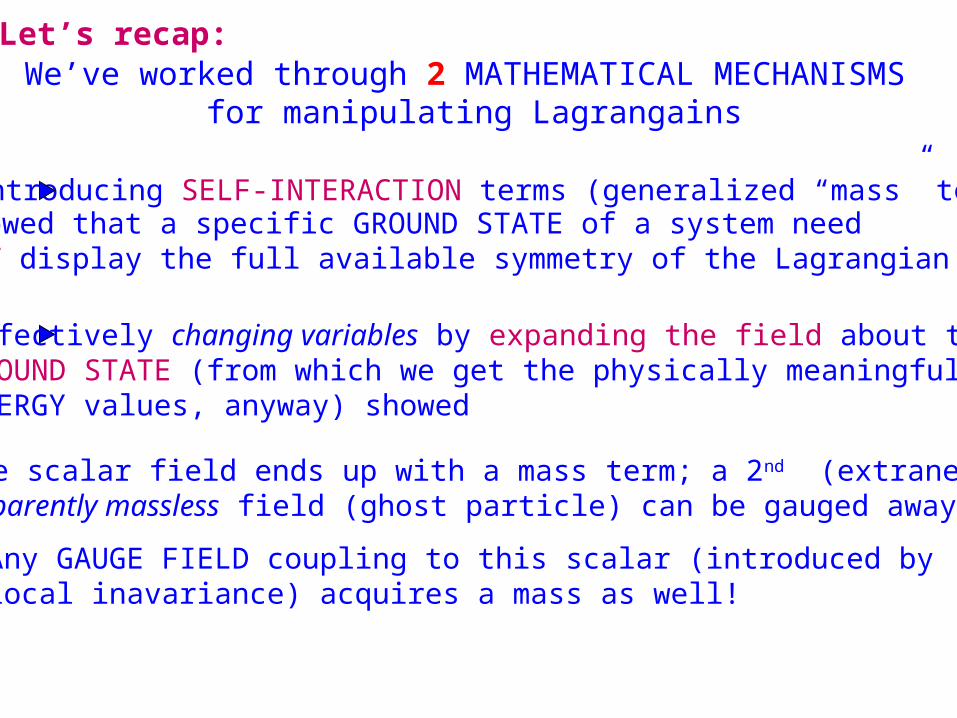
Let’s recap:We’ve worked through 2 MATHEMATICAL MECHANISMS

for manipulating Lagrangains

Introducing SELF-INTERACTION terms (generalized “mass” terms)showed that a specific GROUND STATE of a system need NOT display the full available symmetry of the Lagrangian

Effectively changing variables by expanding the field about the GROUND STATE (from which we get the physically meaningful ENERGY values, anyway) showed

•The scalar field ends up with a mass term; a 2nd (extraneous) apparently massless field (ghost particle) can be gauged away.

•Any GAUGE FIELD coupling to this scalar (introduced by local inavariance) acquires a mass as well!

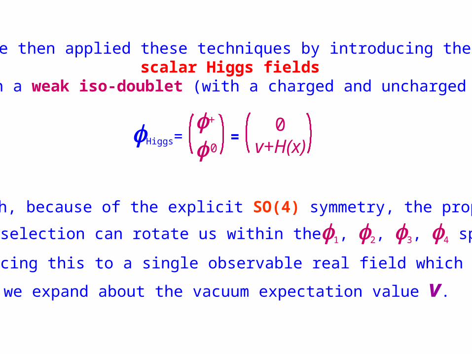
We then applied these techniques by introducing the scalar Higgs fields

through a weak iso-doublet (with a charged and uncharged state)

+

0Higgs=

0v+H(x)

=

which, because of the explicit SO(4) symmetry, the proper

gauge selection can rotate us within the1, 2, 3, 4 space,

reducing this to a single observable real field which we we expand about the vacuum expectation value v.

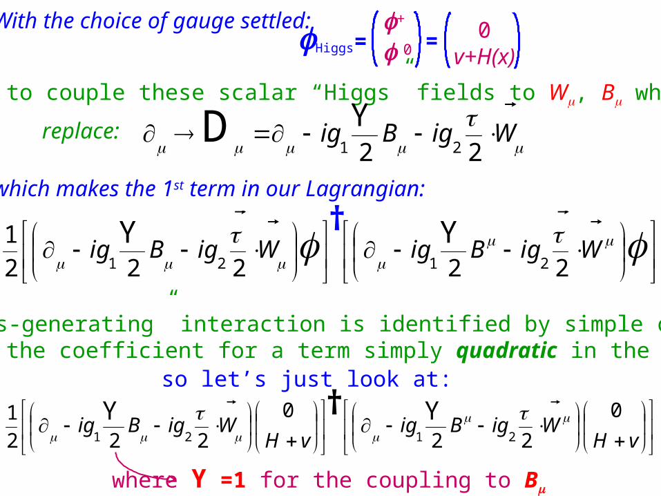
With the choice of gauge settled: +

0Higgs=0

v+H(x)=

Let’s try to couple these scalar “Higgs” fields to W, B which means

WigBig

22 21

YDreplace:

which makes the 1st term in our Lagrangian:

WigBigWigBig

22222

12121

YY †

The “mass-generating” interaction is identified by simple constantsproviding the coefficient for a term simply quadratic in the gauge fields

so let’s just look at:

vHWigBig

vHWigBig

0

22

0

222

12121

YY †

where Y =1 for the coupling to B

vHWigBig

vHWigBig

0

22

10

22

1

2

12121

†

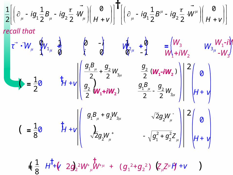
recall that

τ ·W→ →

= W1 + W2 + W30 11 0

0 -ii 0

1 00 -1

= W3 W1iW2

W1iW2 W3

12

= ( )

3

21

22W

gBg

2

321

22W

gBg

)(2

2 g

)(2

2 g

0

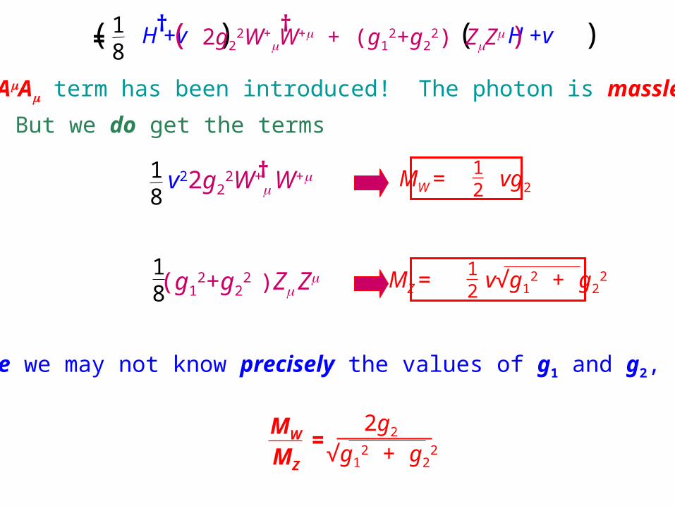
H + v0 H +v

18

= ( ) 321

WgBg 2

Zgg 2

2

2

1

Wg2

2 0

H + v0 H +v

†

†

18

= ( )H +v† ( )H +v

W1iW2

W1iW2

Wg2

2

( 2g22W+

W+ + (g12+g2

2) ZZ )†

18

= ( )H +v† ( )H +v( 2g22W+

W+ + (g12+g2

2) ZZ )†

No AA term has been introduced! The photon is massless!

But we do get the terms

18

v22g22W+

W+† MW = vg2

18 (g1

2+g22 )Z Z MZ = v√g1

2 + g221

2

MW

MZ

2g2

√g12 + g2

2

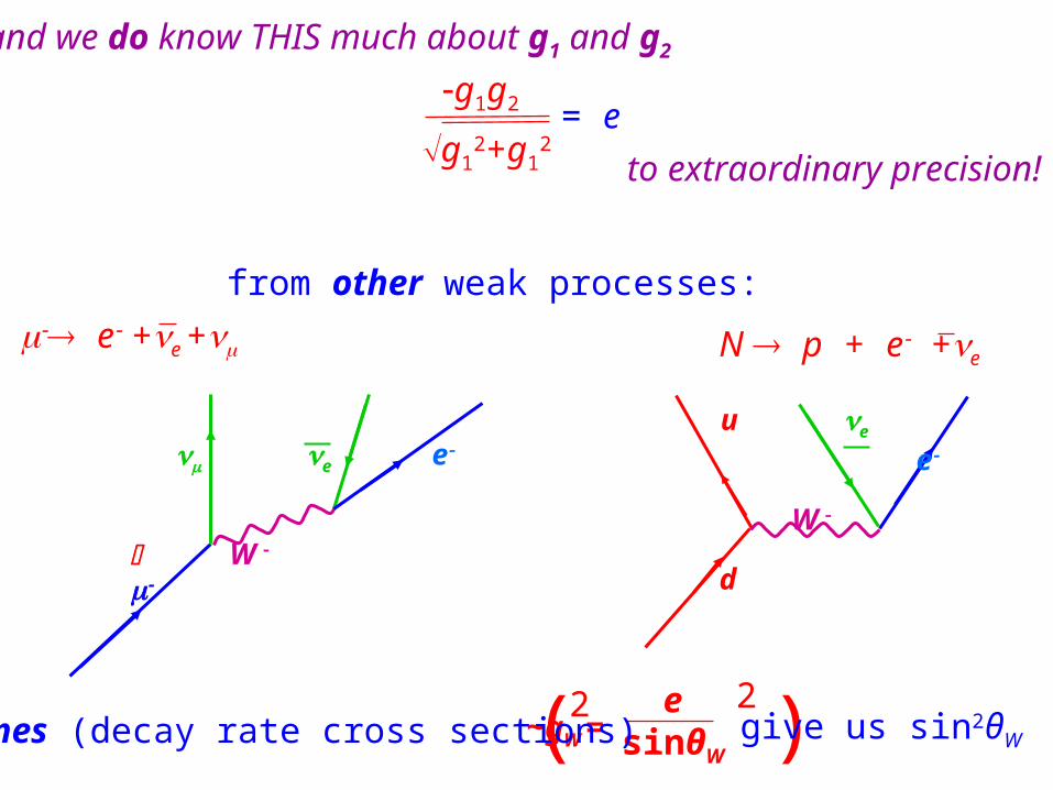
At this stage we may not know precisely the values of g1 and g2, but note:

=

12

e e

W

u e

e

W

d

e+e + N p + e+e

~gW =e

sinθW( )2 2

g1g2

g12+g1

2 = e

and we do know THIS much about g1 and g2

to extraordinary precision!

from other weak processes:

lifetimes (decay rate cross sections) give us sin2θW

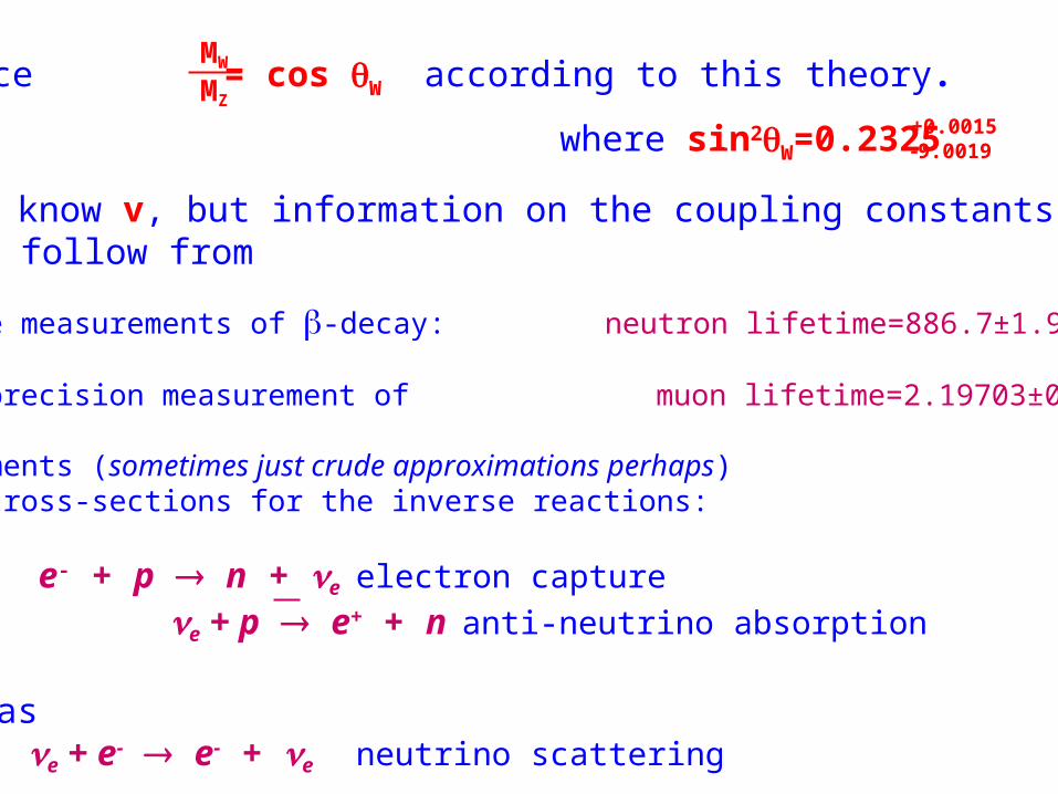
Notice = cos W according to this theory.MW

MZ

where sin2W=0.2325 +0.00159.0019

We don’t know v, but information on the coupling constants g1 and g2 follow from

• lifetime measurements of -decay: neutron lifetime=886.7±1.9 sec and • a high precision measurement of muon lifetime=2.19703±0.00004 sec and • measurements (sometimes just crude approximations perhaps) of the cross-sections for the inverse reactions:

e- + p n + eelectron capture

e + p e+ + n anti-neutrino absorption

as well as e + e- e- + e neutrino scattering

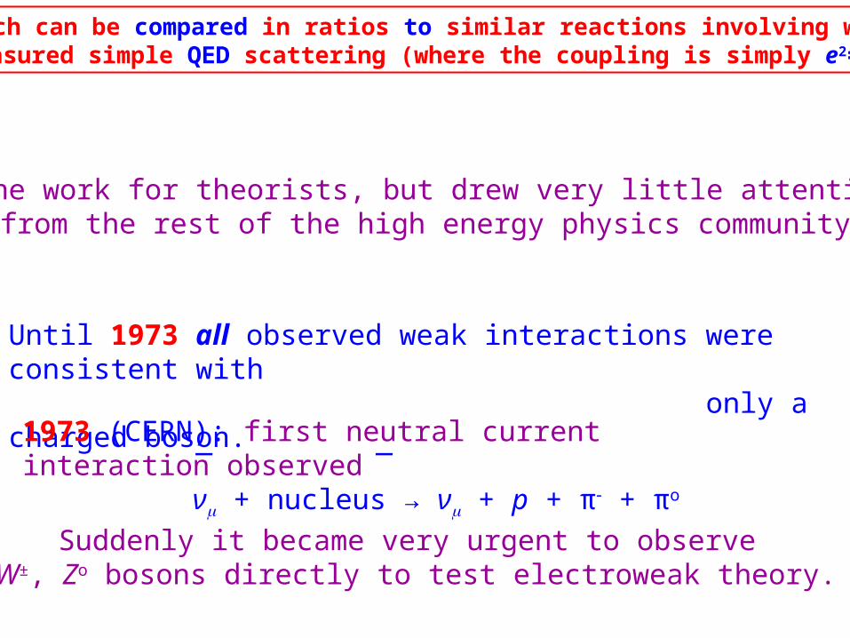
Until 1973 all observed weak interactions were consistent with only a charged boson.

All of which can be compared in ratios to similar reactions involving well-known/well-measured simple QED scattering (where the coupling is simply e2=1/137).

Fine work for theorists, but drew very little attentionfrom the rest of the high energy physics community

1973 (CERN): first neutral current interaction observed ν + nucleus → ν + p + π + πo

Suddenly it became very urgent to observe W±, Zo bosons directly to test electroweak theory.

_ _

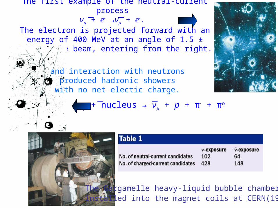
The Gargamelle heavy-liquid bubble chamber, installed into the magnet coils at CERN(1970)

The first example of the neutral-current process νμ + e →νμ + e.

The electron is projected forward with an energy of 400 MeV at an angle of 1.5 ± 1.5° to the beam, entering from the right.

ν + nucleus → ν + p + π + πo

__

_ _

and interaction with neutronsproduced hadronic showerswith no net electic charge.

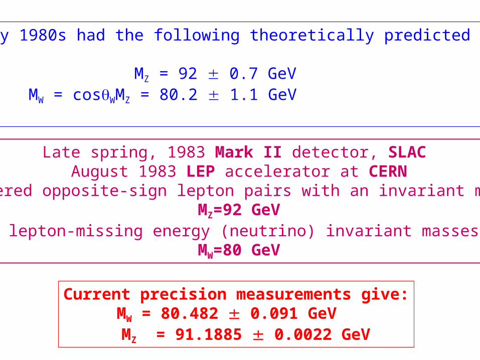
By early 1980s had the following theoretically predicted masses:

MZ = 92 0.7 GeV MW = cosWMZ = 80.2 1.1 GeV

Late spring, 1983 Mark II detector, SLAC August 1983 LEP accelerator at CERN

discovered opposite-sign lepton pairs with an invariant mass ofMZ=92 GeV

and lepton-missing energy (neutrino) invariant masses ofMW=80 GeV

Current precision measurements give: MW = 80.482 0.091 GeV MZ = 91.1885 0.0022 GeV

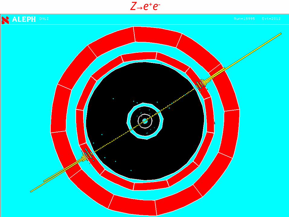
Z→e+e

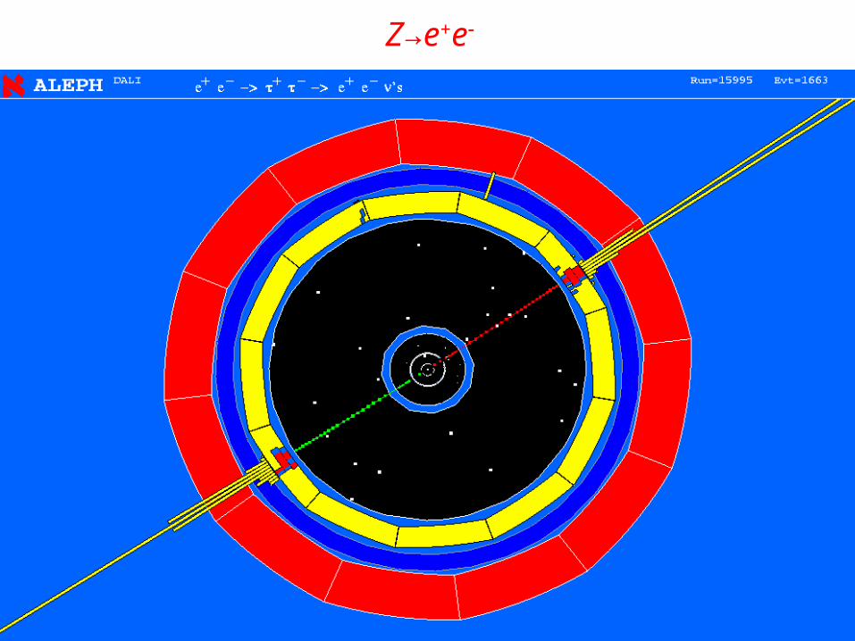
Z→e+e

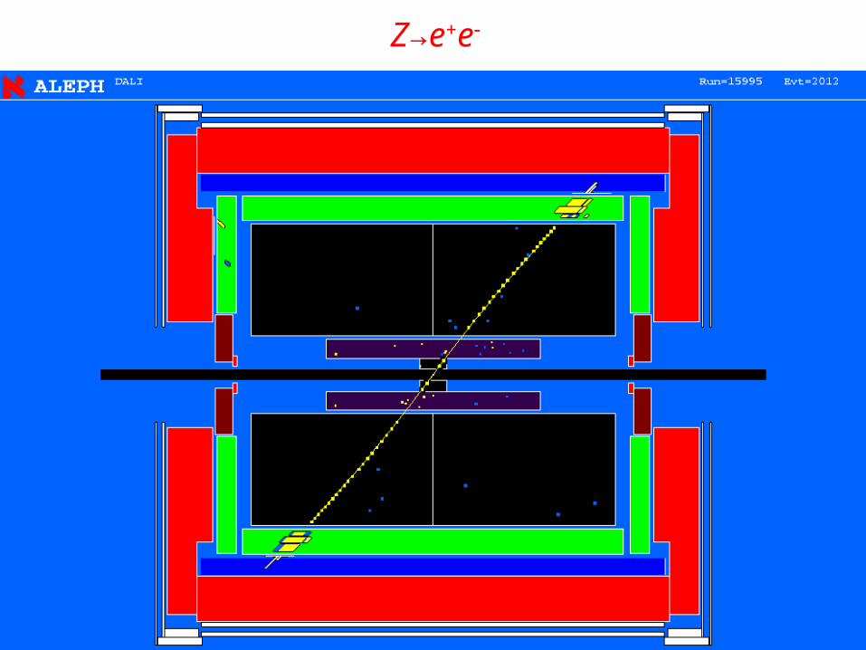
Z→e+e

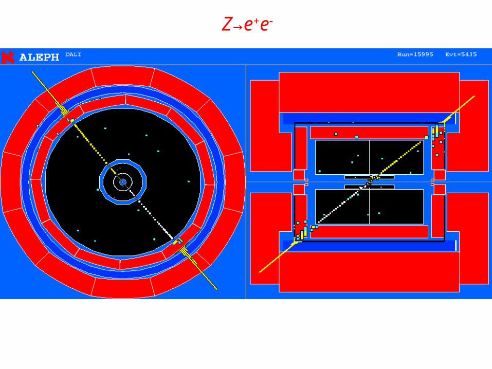
Z→e+e

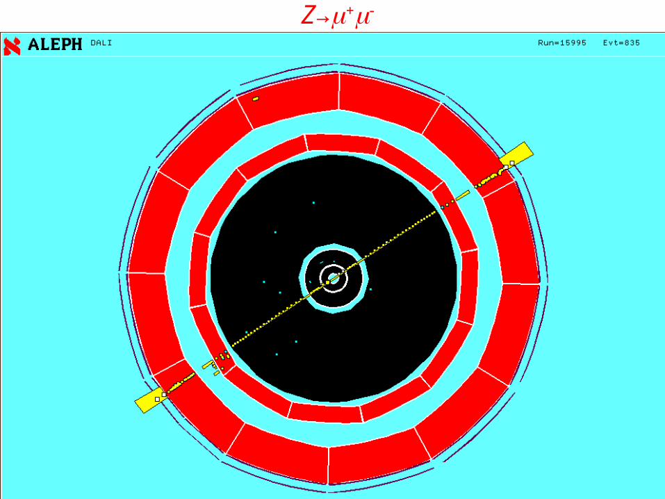
Z→+

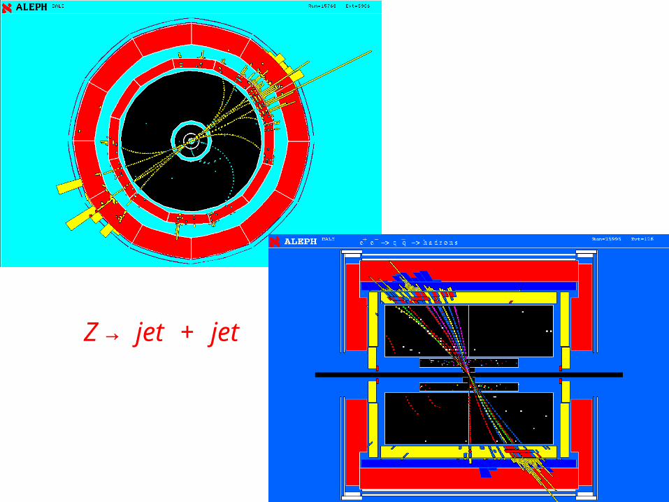
Z → jet + jet

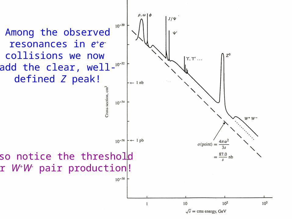
Among the observedresonances in e+e

collisions we now add the clear, well-

defined Z peak!

Also notice the thresholdfor W+W pair production!

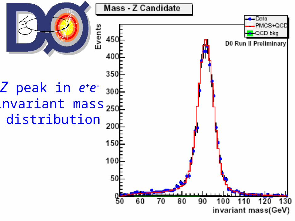
Z peak in e+e invariant mass

distribution

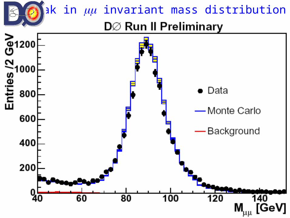
Z peak in invariant mass distribution

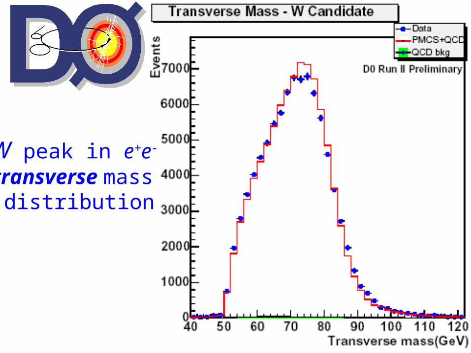
W peak in e+e transverse mass

distribution

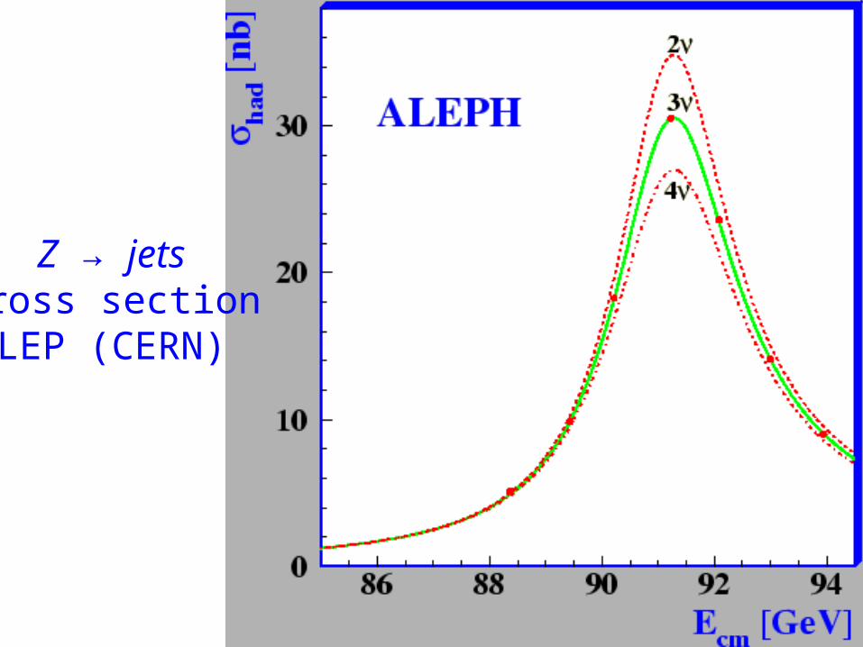
Z → jetscross sectionLEP (CERN)

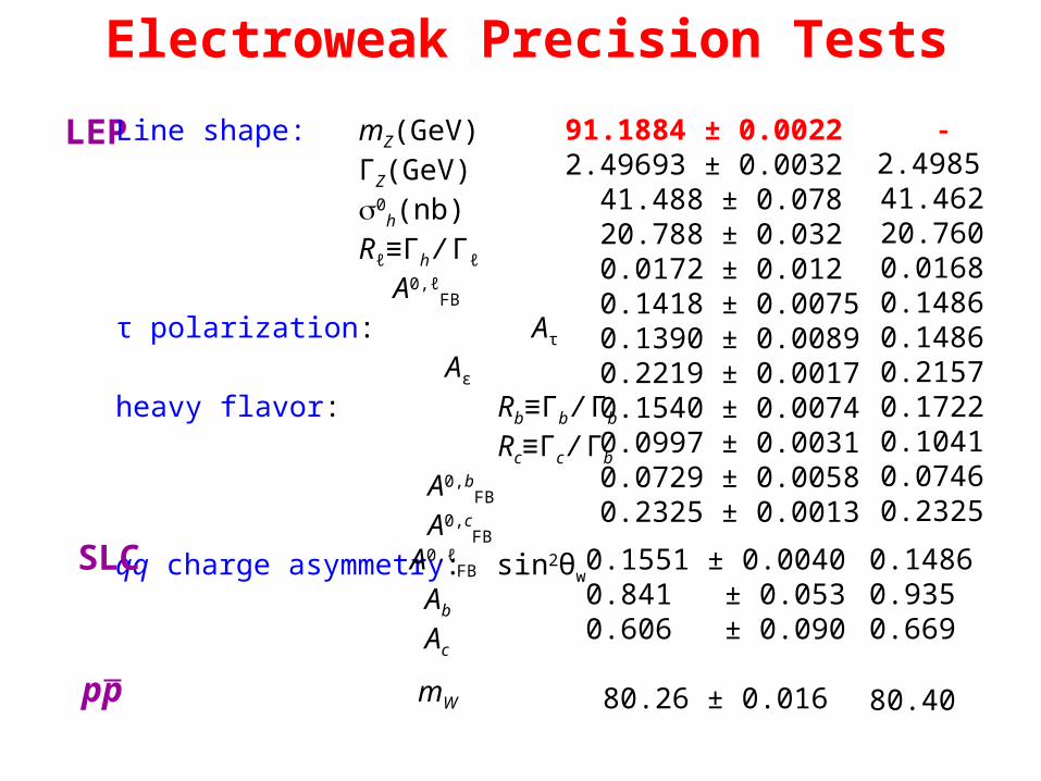
Electroweak Precision Tests

LEP Line shape: mZ(GeV) ΓZ(GeV) 0

h(nb) Rℓ≡Γh / Γℓ

A0,ℓFB

τ polarization: Aτ

Aε

heavy flavor: Rb≡Γb / Γb

Rc≡Γc / Γb

A0,bFB

A0,cFB

qq charge asymmetry: sin2θw

91.1884 ± 0.00222.49693 ± 0.0032 41.488 ± 0.078 20.788 ± 0.032 0.0172 ± 0.012 0.1418 ± 0.0075 0.1390 ± 0.0089 0.2219 ± 0.0017 0.1540 ± 0.0074 0.0997 ± 0.0031 0.0729 ± 0.0058 0.2325 ± 0.0013

2.4985 41.462 20.760 0.0168 0.1486 0.1486 0.2157 0.1722 0.1041 0.0746 0.2325

SLC A0,ℓFB

Ab

Ac

pp mW

0.1551 ± 0.00400.841 ± 0.0530.606 ± 0.090

80.26 ± 0.016

0.14860.9350.669

80.40

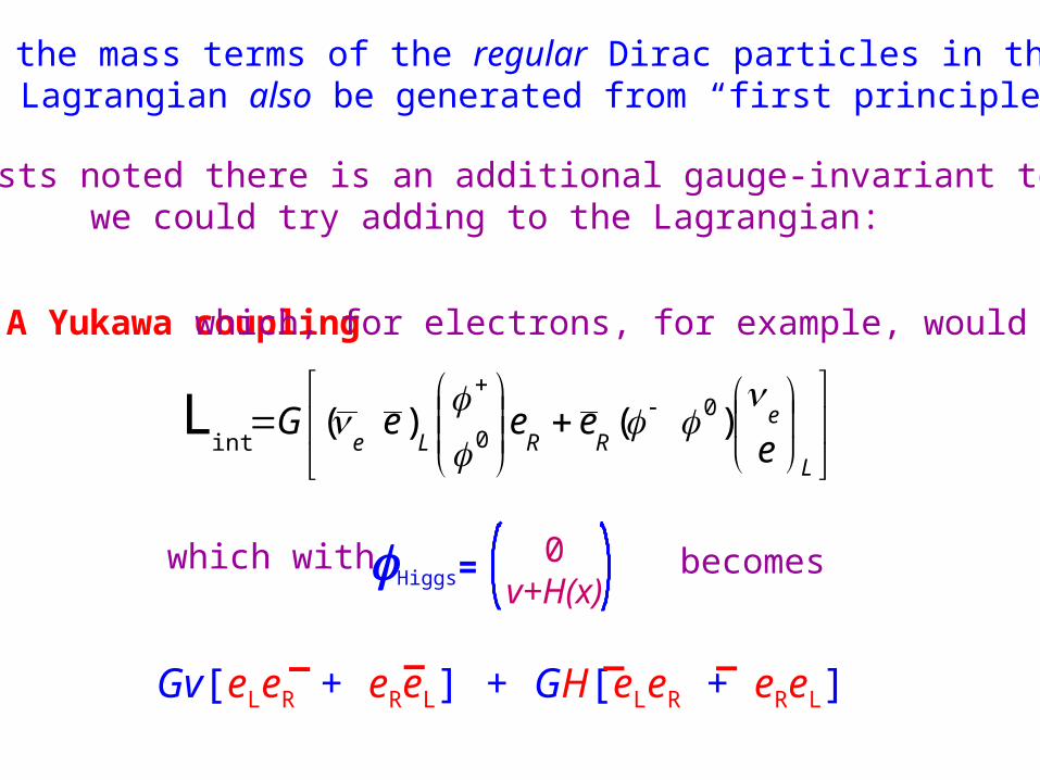
Can the mass terms of the regular Dirac particles in theDirac Lagrangian also be generated from “first principles”?

Theorists noted there is an additional gauge-invariant termwe could try adding to the Lagrangian:

A Yukawa coupling which, for electrons, for example, would read

L

eRRLe e

eeeG

)()( 0

0int L

which with Higgs=0

v+H(x)becomes

Gv[eLeR + eReL] + GH[eLeR + eReL] _ _ _ _

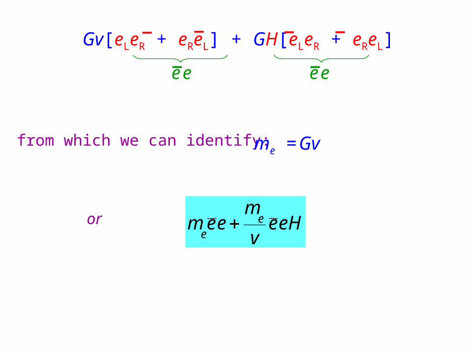
e e_

e e_

from which we can identify: me = Gv

or eHev

meem e

e

Gv[eLeR + eReL] + GH[eLeR + eReL] _ _ _ _

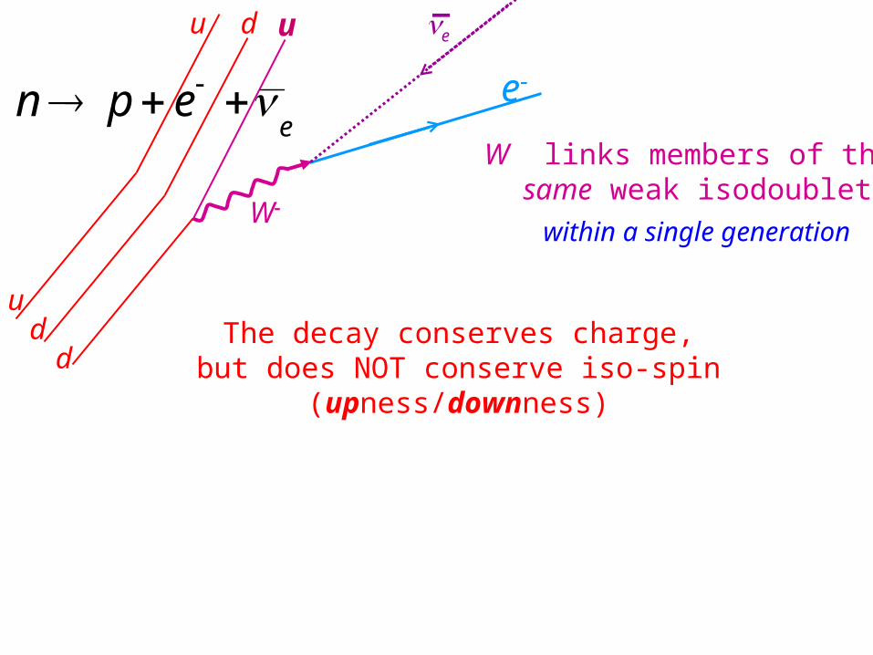
u

d

e

e

_uu

dd

eepn

W

W links members of the same weak isodoublet

within a single generation

The decay conserves charge,but does NOT conserve iso-spin

(upness/downness)

u

d

ee

_uu

dd

eepn

W

However, we even observe some strangeness-changing weak decays!

d uu

du

s

p

du

Ku ds

ss

s

su_

_

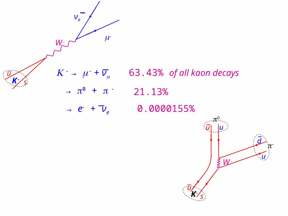
→ + ν 63.43% of all kaon decays

→ 0 + 21.13%

_

→ e + νe

_0.0000155%

u sK

νe

W

u sK

u u

W

u

d

_

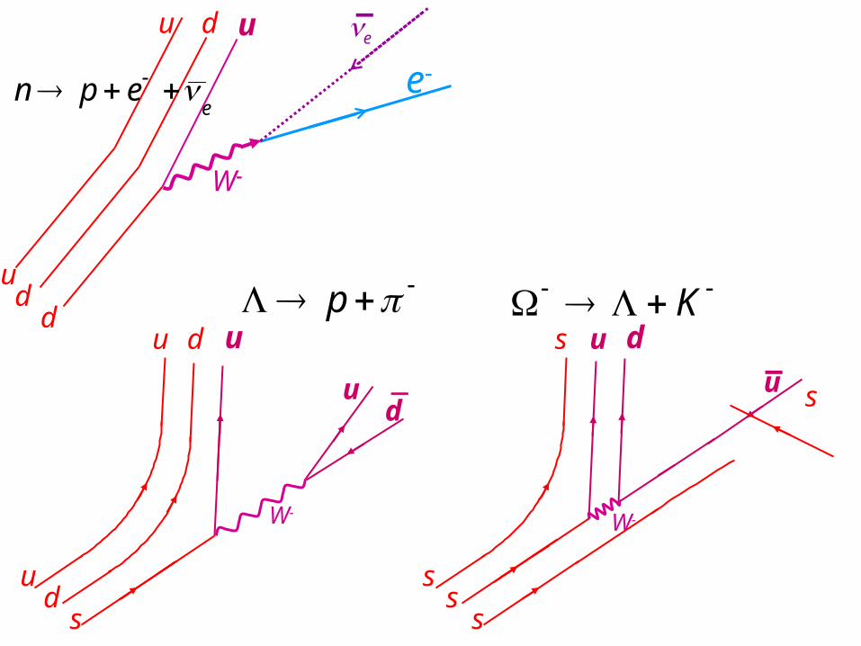
u

d

ee

_uu

dd

eepn

W

d uu

du

s

p

du

Ku ds

ss

s

su_

W

_

W

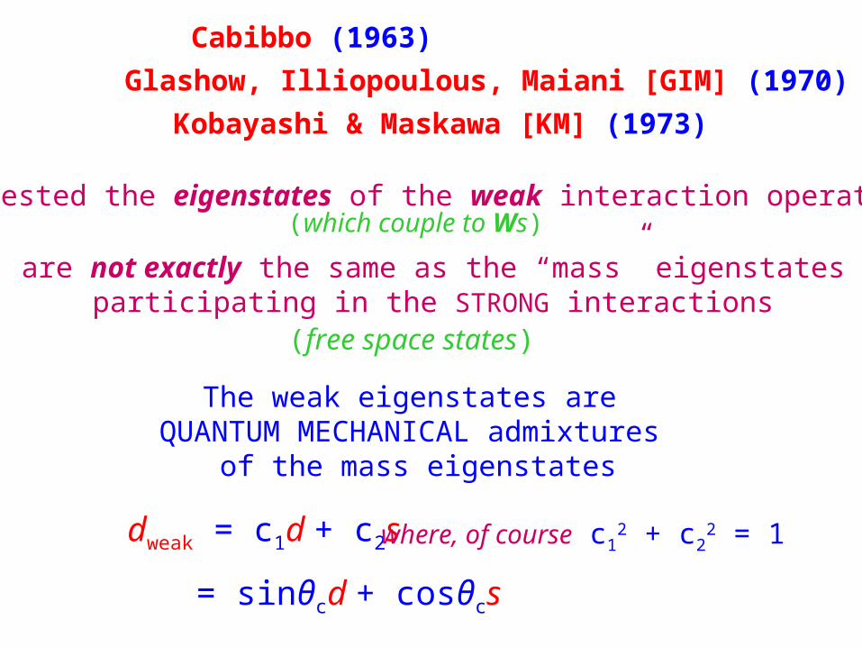
Cabibbo (1963)

Glashow, Illiopoulous, Maiani [GIM] (1970)

Kobayashi & Maskawa [KM] (1973)

Suggested the eigenstates of the weak interaction operators(which couple to Ws)

are not exactly the same as the “mass” eigenstatesparticipating in the STRONG interactions

(free space states)

The weak eigenstates are QUANTUM MECHANICAL admixtures

of the mass eigenstates

dweak = c1d + c2s where, of course c12 + c2

2 = 1

= sinθcd + cosθcs

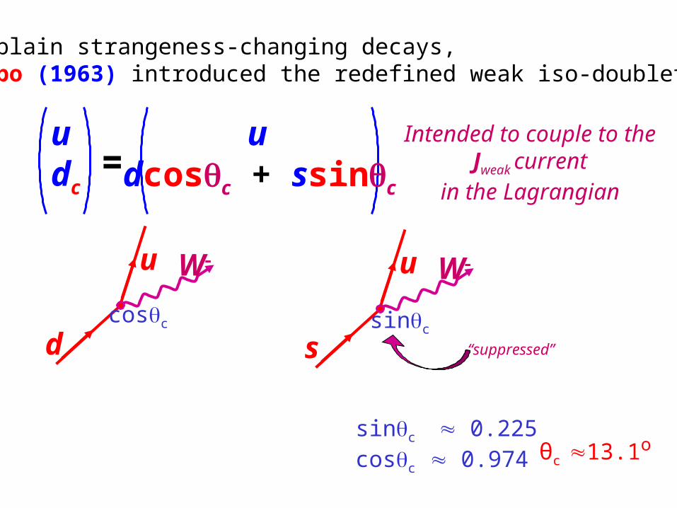
To explain strangeness-changing decays, Cabibbo (1963) introduced the redefined weak iso-doublet

udc

=u Intended to couple to the

Jweak current in the Lagrangian

u

d

W

cosc

u

s

W

sinc

“suppressed”

sinc 0.225cosc 0.974

dcosc + ssinc

θc 13.1o

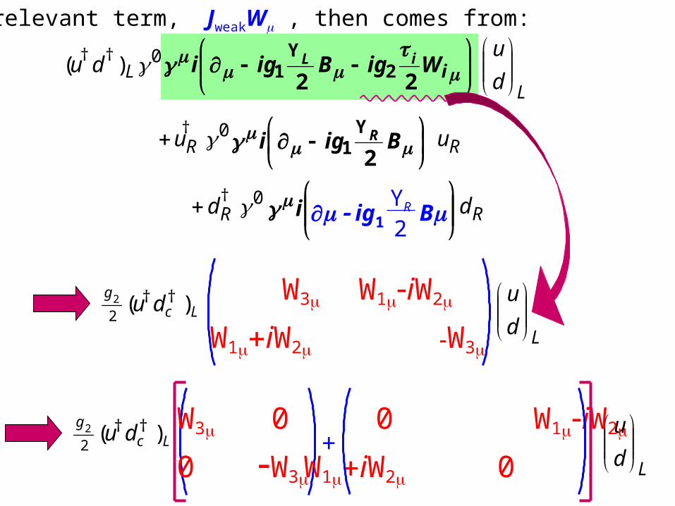
The relevant term, JweakW , then comes from:

iWigBigi iL

22 21

Y0)( Ldu† †

Ld

u

Bigi R

21Y0Ru †

Ru

i0Rd †

Rd ig1 BYR

2

Lcg

du )(22 † †

Ld

u

W3 W1iW2

W1iW2 W3

Lcg

du )(22 † †

Ld

u

W3 0

0 W3

0 W1iW2

W1iW2 0+

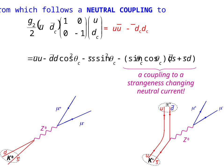
From which follows a NEUTRAL COUPLING to

c

c d

udu

g

10

01

22 = uu - dcdc

_ _

))(cos(sinsincos 22 dssdssdduucccc

d sK

0

Z 0

a coupling to astrangeness changing

neutral current!

u sK+

u d+

Z 0

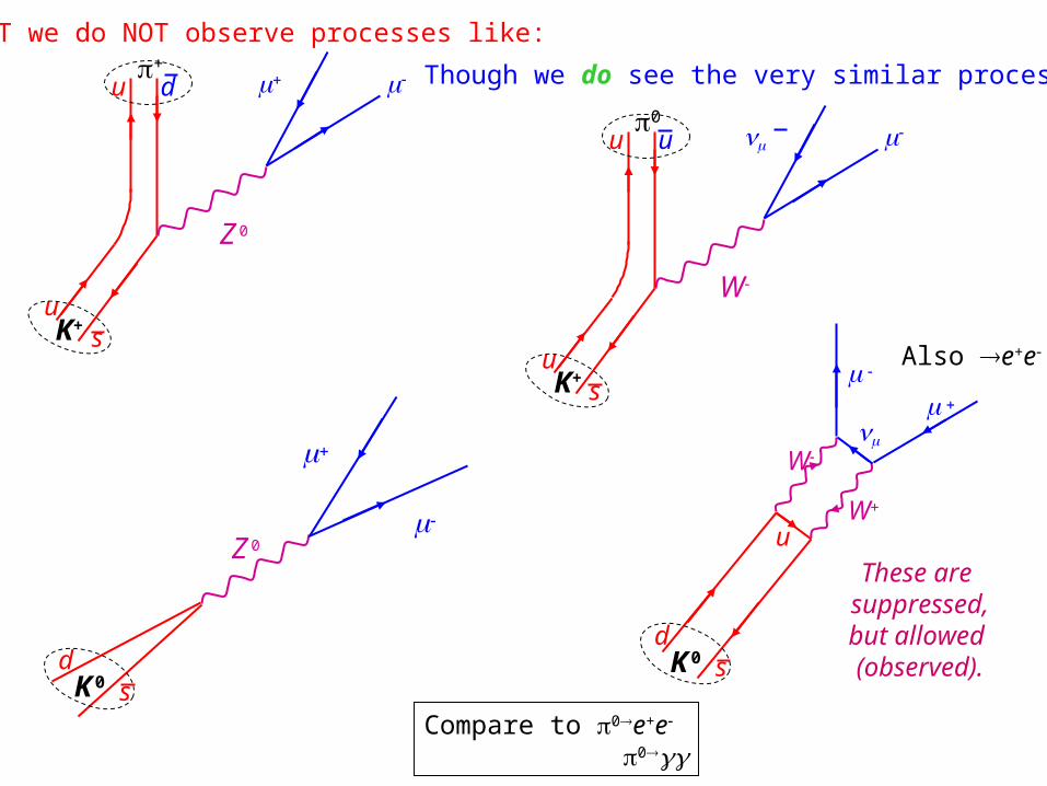
BUT we do NOT observe processes like:

u sK+

u d Though we do see the very similar processes:+

Z 0

u sK+

u u0

W

d sK

0

u

W

W

d sK

0

Z 0

These are suppressed,but allowed (observed).

Compare to 0e+e

0

Also e+e

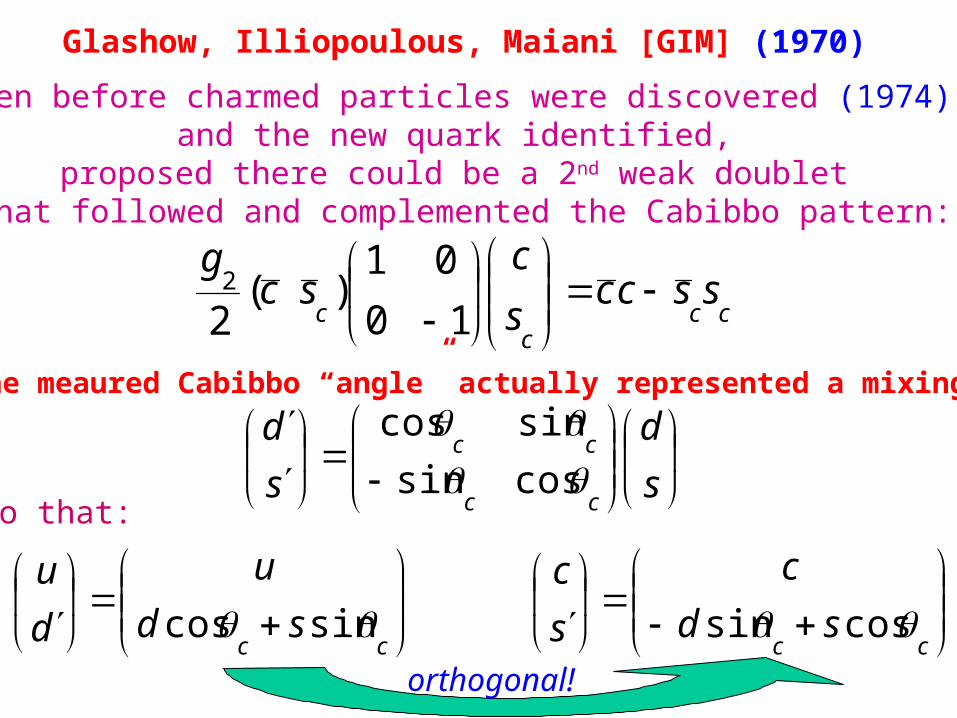
Glashow, Illiopoulous, Maiani [GIM] (1970)

even before charmed particles were discovered (1974) and the new quark identified,

proposed there could be a 2nd weak doublet that followed and complemented the Cabibbo pattern:

ccc

csscc

s

csc

g

10

01)(

22

So that the meaured Cabibbo “angle” actually represented a mixing/rotation!

s

d

s

d

cc

cc

cossin

sincos

so that:

ccsd

u

d

u

sincos

ccsd

c

s

c

cossin

orthogonal!

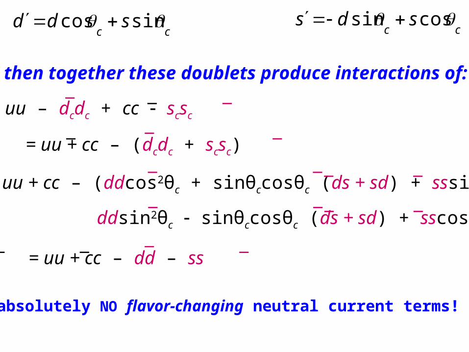
then together these doublets produce interactions of:

uu – dcdc + cc scsc

_ _ __

= uu + cc – (dcdc + scsc)

= uu + cc – (ddcos2θc + sinθccosθc (ds + sd) + sssin2θc

_ _ __

ccsdd sincos

ccsds cossin

ddsin2θc sinθccosθc (ds + sd) + sscos2θc)

= uu + cc – dd – ss_ _ __

_ _ _ _

_ _ _ _

absolutely NO flavor-changing neutral current terms!

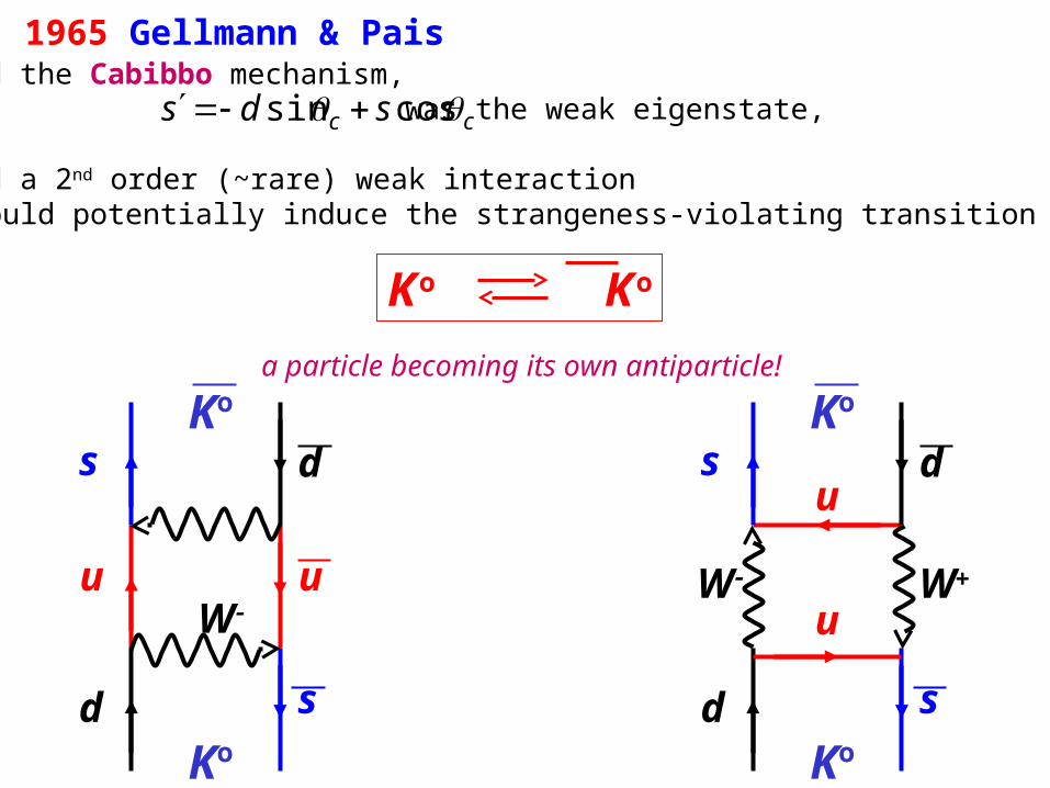
1965 Gellmann & PaisNoticed the Cabibbo mechanism, where was the weak eigenstate,

allowed a 2nd order (~rare) weak interaction that could potentially induce the strangeness-violating transition of

cc sds cossin

K o K

o

a particle becoming its own antiparticle!

u u

s

d s

d

Ko

Ko

W

u

u

s

d s

d

Ko

Ko

W W