Lethal Model 2: The Limits to Growth Revisited · WILLIAM D. NORDHAUS Yale University Lethal Model...

WILLIAM D. NORDHAUS Yale University

Lethal Model 2:

The Limits to Growth Revisited

Two DECADES AGO, a ferocious debate erupted about the feasibility and desirability of future economic growth. The popular imagination was captured by a study of the world economy known as The Limits to Growth.' This work, sponsored by the mysterious-sounding Club of Rome, convinced many that unfettered economic growth had come to an end and that the world was entering the "era of limits."

The emergence of the anti-growth school was the latest peak in a long intellectual cycle of pessimism about economic growth that originated with Reverend T.R. Malthus in the early 1800s. But such concerns receded from the public consciousness in the 1970s and early 1980s as the immediacy of skyrocketing oil prices, a growing international debt crisis, mounting fiscal imbalances, and slowing productivity and real wage growth displaced vaguer long-term anxieties about declining resources and growing entropy.

At the end of the long economic expansion of the 1980s, with stagfla- tion subdued, concerns about long-run viability reemerged, but this time with different emphases. The major concerns of today's critics of growth are not inadequate resources, but excessive consumption. Two decades ago, a Newsweek cover captured the zeitgeist of the times: an empty cornucopia and a headline that stated that the world was "Run- ning Out of Everything." Then, people fretted about factories grinding

I am grateful for comments from the Brookings Panel and from Herman Daly, Gary Haller, Dennis Meadows, and Donella Meadows as well as for research assistance from Agnieszka Ziemba.

1. The seminal work was a methodological tract by Jay Forrester (1971). This was developed with supporting evidence by Donella Meadows and others (1972).

1

2 Brookings Papers on Economic Activity, 2:1992

to a halt as oil wells ran dry. Today's apocalyptic scenarios feature economies and ecosystems disrupted by smoke-belching factories and swel- tering climates overheated by greenhouse gases.

Greenhouse warming is but one of the new environmental ailments that may be by-products of economic growth. Other global concerns include increasing evidence of widespread damage from acid rain; the ap- pearance of the "ozone hole" in the Antarctic, along with ozone depletion in temperate regions; deforestation, especially in the tropical rain forests, which may upset the global ecological balance; soil erosion, which threatens the long-term viability of agriculture; and the extinction of species, which, among other things, threatens to impede future advances in medical and other technologies. On top of these global issues are the more mundane-but probably more lethal-issues of air, water, and soil pollution.

Economists have often belied their tradition as the dismal science by downplaying both earlier concerns about the limitations from exhaustible resources and the current alarm about potential environmental catastrophe. However, to dismiss today's ecological concerns out of hand would be reckless. Because boys have mistakenly cried "wolf' in the past does not mean that the woods are safe. In the sections that follow, I will discuss some of the major concerns about economic growth from both theoretical and empirical points of view. I will use the limits-to- growth debate as a reference point to understand the earlier debate about the limits to and perils of growth, and to provide some perspective about the newer debate about environmental threats.

Background to the Debate

The 1972 version of the Limits to Growth (hereafter known as Limits 1) had its origin in increasing concern about the sustainability of economic growth in a finite world. The debate found an eager audience because of the concerns in the early 1970s about rapid population growth and increasing pollution in developing countries and-after 1973-up- wardly spiraling oil prices and sharply declining growth in output and living standards in the major industrial countries.

Limits I did not sprout in an intellectual desert. Although the limits- to-growth (LTG) studies received the most attention-and criticism-in

William D. Nordhaus 3

the popular press, a quieter and more profound scientific revolution was also underway. Sober scientific analyses such as the Study of Critical Environmental Problems identified a number of potentially important global issues, particularly climate change, and suggested a modest change in priorities necessary to meet the problems.2

However, the approach taken in Limits I concentrated primarily on the classic economic questions raised by Malthus and David Ricardo- questions of induced population growth and diminishing returns to labor with fixed land. The ultimate message was that so many constraints operate on the global economy that there is no way to wriggle out of the straitjacket of resource limitations. In the next section, I will sketch a model of economic growth that will show how the various constraints in the limits-to-growth models operate to send humanity back to the living standards of the Dark Ages.

Evolution of Views

In the two decades since Limits I, the anti-growth message has mu- tated. Criticisms of the Limits I view made by economists and engineers have convinced many that two major factors-technological change and the market mechanism-can prevent the scarcity of appropriable natural resources from constituting a significant drag on long-term economic growth.

At the same time, economists have not been able to vouchsafe that the invisible hand can automatically solve environmental problems. Al- though in principle governments could internalize pollution externalities through such devices as effluent taxes or auctionable quotas, legislators have proved immune to these ideas. Studies of the efficiency of actual regulatory approaches to controlling externalities have consistently found that regulations have been poorly designed and that the costs of control have far exceeded the estimated benefits of efficient policies.'

By the early 1990s, a new vision of the long-run limits to growth was developing among environmental economists and economically minded environmentalists and scientists. The new view holds that long-run constraints upon economic growth might well exist, but that these are un-

2. Study of Critical Environmental Problems (1970). 3. See Tietenberg (1988).


likely to arise because of intrinsic limitations of natural resources. Rather, the limitations would be more likely to arise from one of two other factors, both involving market failures. One possibility is that the scale of human activity could overwhelm the capacity of the globe to tol- erate industrial wastes; this, in turn, could drive the cost of reducing or recycling wastes to astronomical levels. This is the "scale limit." A second possibility is the "political limit." While reducing harmful side effects is in principle possible at modest cost, human societies might lack the political will or skill to take measures to internalize the externalities.

Among those who hold the new view of the limits to growth are the nervous and the relaxed. The nervous include many from the environmental community, which is becoming increasingly hostile to economic growth in poor and rich countries, alike. Our planet is under siege, and humans are the major enemy, the argument runs. The World Commis- sion on Environment and Development (the Brundtland Commission) wrote: Nature is bountiful, but it is also fragile and finely balanced. There are thresholds that cannot be crossed without endangering the basic integrity of the system. Today we are close to many of these thresholds; we must be ever mindful of the risk of endangering the survival of life on Earth.4

Priorities of environmentalists are sometimes at variance with traditional economic approaches, as in the statement by a Canadian environmental group, the Saskatchewan Environment Society: We are deep-air animals living inside an ecological system.... The mainte- nance of the ecosphere is . . . the first priority. Economic development must be secondary, guided by strict ecological standards.'

The dangers of economic development is a theme of the limits-to-growth research team, recycled for the 1992 publication, Beyond the Limits (hereafter known as Limits II): Human use of many essential resources and generation of many kinds of pollutants have already surpassed rates that are physically sustainable. Without significant reductions in material and energy flows, there will be in the coming decades an uncontrolled decline in per capita food output, energy use, and industrial production.6

4. World Commission on Environment and Development (1987, pp. 32-33). 5. From a statement by Stanley Rowe at the public hearing of the World Commission

on Environment and Development, Ottawa, May 26-27, 1986, cited in World Commission on Environment and Development (1987, p. 293).

6. Meadows, Meadows, and Randers (Limits II) (1992, p. xv).


Economists, on the other hand, tend to be at the relaxed end of the spectrum, perhaps because they see so many other horrors. One of the severest critics of the older Malthusian view was Wilfred Beckerman, who had especially harsh words for Limits I. In a recent essay, he puts forth the new view of limits eloquently: [T]he important environmental problems for the 75 percent of the world's population that live in developing countries are local problems of access to safe drinking water or decent sanitation, and urban degradation. Furthermore, there is clear evidence that. . . in the end the best-and probably the only-way to at- tain a decent environment in most countries is to become rich.7

Limits II

The purpose of the 1992 version, Beyond the Limits, was primarily to "update" the earlier version. I was curious to see how the profound developments in economics, science, and technology had influenced the approach. I was disappointed. The new version turns out to be "Lethal Model 2" with the same cast, plot, lines, and computerized scenery.

To refresh the memories of those who have forgotten or inform those who never knew, I will outline the basic structure of the LTG model and sketch its basic conclusions. The basic structure is an aggregate model of the world economy. The model takes the form of a system of nonlinear difference equations, most of them being first-order. The system can be written succinctly as

(1) Y,= F(Y, ,Z, P),

where t is time; Y, is the set of endogenous variables, approximately 150 in number, of which the most important are population, pollution, food, industrial output, and nonrenewable natural resources; Z, represents the exogenous variables; and ,3 represents the system's parameters.

The model's structure was basically determined in the 1972 vintage and, with some exceptions, was retained in its entirety for the 1992 vintage. The authors represented advances in economic and scientific understanding since 1972 by seven changes. First, Limits II reduced the "lifetime" of land from 6000 years to 1000 years because of increased erosion. Second, the new version slightly changed the (time-invariant) agricultural production function because of increases in land productiv-

7. Beckerman (1992, p. 482).


ity. Third, the 1992 text shifted the (time-invariant) function relating resource use to output downward to reflect the observed decline in resource use per unit of output. Fourth, the authors allowed industrial capital to be invested in pollution-abatement technology. Finally, Limits II lowered birth rates, decreased desired family size to reflect demographic trends, and increased the impact of health services on life expec- tancy.8

FINDINGS. The modified model was then used to create scenarios to describe the possible evolution of the world economy. The findings of Limits I were dismal: If present growth trends in world population, industrialization, pollution, food production, and resource depletion continue unchanged, the limits to growth on this planet will be reached sometime within the next one hundred years. The most probable result will be a rather sudden and uncontrollable decline in both population and industrial capacity.9

With little change in the structure of the LTG model, it is not surprising that the results of Limits II differ little from those of Limits I. The baseline scenario is one in which "the world society proceeds along its historical path as long as possible without major policy change. "'0 The basic scenario shows that per capita food production peaks in 1994 and then falls by 40 percent over the next three decades; that per capita industrial production peaks around 2010, then declines at about 4 percent annually through the 21 st century to a level of about 5 percent of its peak by 2100; and that population goes through a Malthusian crisis, growing rapidly until around 2035, and then declining by over half by the end of the next century.

One question about the LTG models is whether they are robust to alternative specifications. Limits I claimed that the basic mode of overshoot and collapse is an intrinsic feature of the model. Thus [The] present world model . .. has led us to one conclusion that appears to be justified under all the assumptions we have tested so far. The basic behavior mode of the world system is exponential growth of population and capital, followed by collapse. 11

8. The published writings do not contain a description of the model's equations. I gleaned these from a computer program that the authors supplied.

9. Limits I (p. 23). 10. Limits II (p. 131). 11. Limits I (p. 142). Emphasis in original.


The same theme runs through Limits II, although it is more cautious in tone: [T]he model system, and by implication the "real world" system, has a strong tendency to overshoot and collapse. In fact, in the thousands of model runs we have tried over the years, overshoot and collapse has been by far the most fre- quent outcome. 12

I will take up the issue of the system's robustness again later.

Utopia in Limitland

Using the model of Limits II, the authors attempt to lay out a series of steps that would prevent overshoot and collapse. Most of the steps would be noncontroversial, such as using resources more efficiently, increasing land yields, and abating lethal pollution. Some would be controversial but arguably sensible, such as limiting population. The final proposal is so striking that I will quote it in full: [The scenario] shows a simulated world . .. with a definition of "enough." This world has decided to aim for an average industrial output per capita of $350 per person per year-about the equivalent of that in South Korea, or twice the level of Brazil in 1990.... If this hypothetical society could also reduce military expenditures and corruption, a stabilized economy with an industrial output per capita of $350 would be equivalent in material comforts to the average level in Europe in 1990.13

This astonishing passage is one of the few recommendations in Limits II that can be held up to the light of statistical analysis. While the definition of "industrial output" is unclear, the factual predicates of the recommendation are so faulty that one wonders whether Limits II is referring to another planet. 14 A rough estimate of global per capita GNP in 1990

12. Limits II (pp. 136-37). 13. Limits II (pp. 195f). 14. Considerable ambiguity surrounds the meaning of the term "industrial output" in

Limits II. Industrial output would appear to be an input into GNP, but is distinguished from GNP because GNP is "kept in money terms, not physical terms" (Limits II, p. 34). The implicit production function seems to be that industrial output is used to make various kinds of capital and the capital then makes output in different sectors according to fixed capital-output ratios. It appears then that "industrial output" corresponds to GNP.

According to personal communication with one of the authors of Limits II, Dennis Meadows, this passage has been misinterpreted and the $350 figure should apply to "consumer goods" (which I assume to mean consumption of goods and services) in 1968 U.S.


would be $4200, while that of OECD countries would be $20,170. South Korea's per capita GDP in purchasing-power-parity terms in 1990 was $7190, not $350. The per capita GDP of the poorest country in Western Europe, Portugal, was almost $8000 in 1990.15 The Limits II proposals would limit our material aspirations to attaining the living standards of Somalia or Chad. At these income levels, we surely could not afford secondary or college education, a good economics textbook, or the Brook- ings Institution, and to purchase Limits II would take a month's wages. The world could not afford to undertake the investments to slow global warming or the research and development to develop resource-saving technological change. The LTG prescription would save the planet at the expense of its inhabitants.

Limits in Simple Growth Models

Limits I and II are not user-friendly for those who want to peer inside the model's black box. The structure is represented by equations with arbitrary step functions in computer language. Moreover, once the actual specifications are unearthed, they do not conform to either national accounting systems or to standard economic definitions, nor does any explanation occur for the wealth of analytic neologisms. In an earlier paper, I attempted to describe and simulate the structure of LTG-type models. 16 In this section, I will follow a different approach and specify a general model incorporating potential growth limits. Then I will show how the economy can run aground.

dollars. Using the consumption deflator, this statement would then translate into around $1,230 per capita of consumption in 1990. Because personal consumption expenditure is around 65 percent of GNP, this represents per capita GNP of around $1,900 in 1990, which means that the revised statement is off by a factor of 11, as compared to a factor of 58 for the published version. The puzzle about the revised interpretation is that "production of consumer goods" nowhere appears in the model of Limits II. Moreover, the stabilized run refers to stabilizing industrial output, not consumption. Finally, one is tempted to say that, unlike fine wines, old prices sour quickly.

15. Data are from World Bank (1992, table 1, p. 218, and table 30, p. 276). Individual country data are from the United Nations' International Comparison Project estimates, while those for groups of countries use official exchange rates.

16. Nordhaus (1973a).


The General Resource-constrained Model

I will start with a general model of a closed economy (say, the world) that is an extension of the standard neoclassical growth model. It has two outputs and multiple inputs. For simplicity, I omit the time sub- scripts, t, where inessential. The aggregate production function for the economy is given by

(2) Y = G(X, P) = F(L, R, T, K; H),

where Y is real output corrected for pollution and other externalities; X is gross output (GNP); P is pollution (which is a "bad"); L is labor inputs, which are proportional to population; R is the flow of natural resource inputs; T is land inputs; K is capital services, proportional to the capital stock; and H represents the level of technology. G is an index of true national income that corrects for any disamenities, while F is a smooth, neoclassical, constant-returns-to-scale production function in which all inputs have positive marginal products and diminishing returns. In addition, I assume that factors are paid their marginal products.

The model can be conveniently recast by rewriting it in the form of a generalized Cobb-Douglas production function. Any smooth production function of the kind depicted in equation 2 can be written without loss of generality as a power function in which the exponents are the local elasticities of output with respect to the inputs. For notational purposes, I use capital letters to represent the (variable) output elasticities of the generalized Cobb-Douglas production function; I reserve lower- case symbols for the special case of the conventional Cobb-Douglas production function in which the elasticities are constant. Hence equation 2 can be rewritten as follows for the generalized Cobb-Douglas production function:

(3) Y = HLVRA TEKA.

In this representation, the exponents are functions of the factor proportions, so fl = fQ(L, R, T, K; t) = (d Y/dL)LIY, with the analogous rela- tions holding for the other exponents of equation 3.

I will next discuss how the elasticities change over time as a function of the shape of the production function. In this approach, the elasticities in equation 3 are functions of factor proportions and of technological


change. If the elasticities of substitution between pairs of factors are not unity, the output elasticities will change over time.'7 If elasticities of substitution are constant, equal, and less than unity, and if technological change is Hicks-neutral, then the output elasticities will rise over time for the slowest growing input and will fall over time for the fastest growing input. Eventually, in this case, the marginal product of the slowest growing factor will tend toward its average product, which means that its output elasticity and share will tend toward unity. This tendency can be reversed or accelerated to the extent that technological change is not Hicks-neutral.

Although this setup looks quite complicated, it is much simpler than the actual LTG models, which contain time delays, multiple sectors and resources, and other features that obscure, rather than inform, the system. Because the system displays constant returns to scale, fQ, + A, + r, + A, equals one at every point of time. Given the assumptions, the elasticities are equal to their factor shares, which would be fQ, = 0.6; A, = O.1;F, = 0.1;andA, = 0.2 atpresent.

A SIMPLER MODEL. The general resource limits model in equation 3 can be simulated on a computer, but it is fruitful to make some simplifi- cations so that analytical solutions are possible. The model can be simplified without losing any critical properties as follows. First, assume that there is a fixed capital-to-output ratio, v = KIY. This assumption is of little importance and is made in the LTG models. 18 Next, ignore pollution at the outset. Third, assume that land is constant. This is a conventional assumption and is probably a reasonable first approximation to the actual fact.

Finally, assume that there is a fixed initial stock of natural resources, S*. Modeling the allocation of a fixed supply of exhaustible resources over time is a complex problem, and I simplify it by assuming that ,. of the remaining resources are consumed in each period t. This gives

(4) R,= .S*e-I'.

17. For constant-returns-to-scale production functions of the form Y = F(K, L), the elasticity of substitution (between K and L) is defined in terms of the partial derivatives of F as a = FKFLIFKL, where Fj is the partial derivative of F with respect to j and K and L are capital and labor, respectively. A nontechnical review of different definitions of the elasticity of substitution in production functions can be found in Solow (1967).

18. In most cases, if saving is a constant fraction of output, this will lead to a fixed capital-to-output ratio.


Using equation 4 and the other assumptions above, a transformed production function can be derived as follows:

(5) Y, = KHII(I-A)L,/1I(IA-)R tA(I-) = K'HtII - ̂ ) Lt(l - ) e -

where K and K' are inessential parameters. Equation 5 is now easy to analyze. The new initial values of the parameters are Q/(1 - A) = 0.6/(1 - 0.2) = 0.75 and A/(1 - A) = 0.1/(1 - 0.2) = 0.125. Note that the sum of the exponents is 0.875 < 1, which indicates that output has decreasing returns to balanced increases in L and R. This result stems from classical Ricardian diminishing returns in the face of limited supplies of land.

THE SIMPLEST LTG MODEL. An explicit solution for the model can be obtained for the non-Malthusian case in which population growth is constant at rate n. To be faithful to the LTG models, assume that there is no technological change [h = the rate of growth of H = (daH,ht)IH, = 0]. Taking the logarithmic derivative of equation 5 and using the assumption about resource use in equation 4 yields

(6) g = -[1 - f/(1 - A)]n - [A/(1 - A) I

where g is the growth of output per capita. This shows that per capita output growth is the sum of two negative terms. The first negative term is the drag on per capita growth given by diminishing returns. The second is the drag from exhaustible resources. Hence, in this simple example of non-Malthusian demography, living standards decline under the weight of diminishing returns on land and depletion of natural resources. Decline is inevitable, although it might be slower if resources were abundant, population growth were slow, or if nonlabor inputs were unimpor- tant in production.

Lethal Conditions

Like LTG models, the general model given in the last section shows the tendency toward economic decline. In addition, there are no less than four conditions, each of which is satisfied in the LTG model, that will lead to ultimate economic stagnation, decline, or collapse. 19 All four

19. In general, I have ignored the fascination shown in Limits II for overshooting. In multi-equation difference equations of the kind used in LTG models, overshooting will


conditions depend on the absence of either general or resource-saving technological change. Some of these depend upon some inputs being "essential," which is defined as an input whose elasticity of substitution in production with other factors is less than one.20

A return to the Dark Ages or worse is unavoidable under each of the four following conditions. For the first three models, I will assume no pollution exists, while for the fourth model, I will introduce pollution into the analysis.

Lethal Condition 1. With no other binding constraints and essential natural resources, the economy runs out of gas and can find no substitutes. This implies that the share of resources (A) -> 1, so the output growth rate tends to the growth of resources, - ,u (as long as n > - R). That is, the asymptotic growth rate of output equals the rate of decline of inputs of the essential natural resource.

Lethal Condition 2. If land is essential for food production, then the share of land (F) -> 1. Thus output growth tends to 0 and per capita output grows at - n. This is the classical case of diminishing returns.

Lethal Condition 3. In the Malthusian case, assume that population growth responds positively to higher levels of income. This produces a low-level trap in which population is endogenous and tends to that level at which the marginal product of labor equals the subsistence wage. If, in addition, there are essential natural resources (as in Lethal Condition 1), then the population that can be supported at the subsistence wage declines along the path to ultimate extinction.

Lethal Condition 4. Next, introduce pollution and global environmental variables. These models are much more complicated because they involve multiple outputs and questions of the extent of internaliza-

represent the presence of oscillatory solutions, reflecting imaginary roots to the character- istic equation. Given the size of the model, a large number of imaginary roots-and therefore the presence of overshooting-is not surprising.

20. An input that is essential is one in which there is a positive minimum amount required per unit of output. For example, assume that the constant-returns-to-scale unit production function is of the form 1 = F(k, m), where k and m are the capital and labor require- ments per unit of output. As capital increases, less labor will be required. As the amount of capital tends to infinity, and if the labor requirement tends to some m* > 0, then labor is "essential." If m* -O 0 as k -* oo, then labor is "inessential." For production functions that have constant and equal elasticities of substitution between factors, if the elasticities are less than one, each factor is essential; on the other hand, if the elasticities of substitution are greater than or equal to one, no factor is essential.


tion of the externality. In the simplest "flow pollution model" sketched in equation 2, the analysis is simply an extension of the limited resource models in Lethal Conditions 1 and 2.

A more interesting case comes for stock externalities. Take the case in which a pollutant is emitted in fixed proportions with output (this being "essential" pollution). The pollutant accumulates, but is slowly removed by natural processes. Finally, a catastrophic threshold exists, above which the pollutant has unacceptable impacts upon human societies (the civilian equivalent of nuclear winter). The constraints on the system can then be rewritten as

dPldt = vY - otP P'P*,

where P is the stock pollutant, v is the fixed emissions-output ratio, a is the natural rate of removal of the pollutant, and P* is the catastrophic threshold. This system leads to a maximum sustainable output, Y*, of

Y* = a-P*/v.

If population is growing, this would lead to an asymptotic decline in per capita output at the rate of growth of population. Moreover, the only technological change that would prevent the dismal outcome would be pollution-saving technological change. For example, if a catastrophic reaction were to occur from a doubling of carbon dioxide concentrations, and if no improvements in the current C02-output ratio were possible, then (given the parameters of the climate system) world output would ultimately be constrained to slightly above today's level.21 None of the predicates of this argument has been shown to be realistic. How- ever, the example illustrates Lethal Condition 4 well.

WHY SENSITIVITY ANALYSES DO NOT MATTER. The LTG studies contain a number of "sensitivity runs" that ask whether the lethal limits to growth can be avoided. The runs include removing the pollution lim-

21. A doubling of CO2 concentrations would lead to an increase in concentrations of about 600 billion tons of carbon (P* = 600 billion tons carbon); emissions are today about 6 billion tons annually, of which two-thirds are immediately lodged in the atmosphere with a residence time of about 120 years. With these parameters, the steady-state viable emissions would be about 7.5 billion tons per year, or about one-quarter more than today's level. I present a more extensive discussion of optimal growth with catastrophic externalities in a forthcoming work (Nordhaus, forthcoming).


its, doubling the stock of natural resources, doubling agricultural production, and similar tests. It can be seen immediately, without any assistance from supercomputers, that these strategies do not get at the heart of any of the four lethal conditions. It is hardly surprising that dead rabbits are pulled out of the hat when nothing but dead bunnies have been put in.

In addition, this catalogue of lethal conditions can easily obscure the basic point that comes from examining complex growth models-which is that there is no general conclusion. Long-run growth trends depend upon the growth of inputs, the rate and direction of technological change, and the elasticities of substitution among the different factors. Until we have secure knowledge about all these factors, no magic formula or supercomputer can foretell whether growth or stagnation will be the victor in the race between technological change and resource scar- cities.

Critiques of the Club of Rome Models I and II

The dire forecasts of the LTG school were not well received by the economics community. While this computerized dirge for industrialization would probably have found sympathetic ears among the classical economists of the early nineteenth century, modern economists have a different view of the dynamics of economic growth and found little to agree with in the LTG models.22 The criticisms of Limits I were extensive. Moreover, because Limits II is virtually identical to the 1972 vintage, the earlier analyses carry over time to the updated version without spoilage. The major shortcomings include the following:

* Equations and definitions of variables seem to have been invented de novo instead of building on existing scientific knowledge. In Limits I, no attempt was made to estimate the behavioral equations econometri- cally, although some attempt seems to have been made to calibrate some of the equations, such as the population equation, to available data.

* The production structure is pessimistic, particularly with respect to the "essential" nature of different inputs. There is no substitution between abundant inputs and limited factors, such as the severely limited natural resource of land. No pollution abatement was allowed in Limits

22. See Beckerman (1972), Solow (1974), and Nordhaus (1973a).


I, although it is possible in Limits II to reallocate capital to pollution- abatement activities.

* Both models rule out ongoing technological change. In this respect, they are inconsistent with the standard interpretation of economic history during the capitalist era.23

* Both models are enormously complex, with a variety of nonlineari- ties and lags. In light of developments in the understanding of nonlinear systems over the last twenty years, it seems apparent that the dynamic behavior of the enormously complicated Limits I model was not fully understood (or even understandable) by anyone, either authors or critics.24

LIMITS OVERTURNED ON THE SIMPLE GROWTH MODEL. I showed above that the "lethal" nature of economic growth in Limits I and II can be reproduced in simple growth models. I will now show how the entire argument can be reversed with a simple change in the specification of the model; more precisely, I will introduce technological change into the production structure and assume that the Cobb-Douglas production function accurately represents the technological possibilities for substitution. I use lower-case Greek symbols to express the conventional Cobb-Douglas production function (one in which the exponents or elasticities of the previous model are now constant). Hence the production function in equation 3 is written as Y = H LX RI Ty Kb for the conventional Cobb-Douglas case, in which the parameters w, X, y, and 8 are constant and sum to one. To introduce technological change, assume that there is Hicks-neutral technological change at rate h. After suitable transformation, this changes equation 6 to the following:

(7) g = -[I - w/(l - 8)]n - XR/(l - 8) + hl(l - 8),

where g is the growth of output per worker. Then output per capita can grow as long as

(8) h > (I - 8 )n + A>.

To use parameters that are consistent with historical growth, again take the values of w = 0.6, X = 0.1, and 8 = 0.2. With n = 0.01 and R =

23. See particularly Kuznets (1977), Maddison (1982), and Denison (1962, 1967). 24. To the authors' credit, and unlike most models, it was extremely carefully docu-

mented; see Meadows and others (1974).


0.005, to offset the drag from resources and diminishing returns, technological change must satisfy the following:

(9) h > (0.2)0.01 + (0.1)0.005 = 0.0025.

That is, technological change must exceed one-quarter of 1 percent a year to overcome the growth drag in this simple case. Historical rates of total factor productivity, h, in developed countries have been on the order of 0.01 to 0.02, which is well in excess of the rate required to offset resource exhaustion and diminishing returns.25

The discussion to this point and a careful study of the simplified LTG- type model lead to one conclusion that was not always clear in the earlier debate about growth limits. While the LTG school argued that economic decline was inevitable and economists argued that the LTG argument was fallacious, the argument is ultimately an empirical matter. Put differently, critics would have gone too far had they claimed that the postu- lated pessimistic scenario could not hold. Perhaps the LTG school had little appreciation for the invisible hand. On the other hand, even a perfectly functioning price system could not prevent ultimate economic decline if any of the "lethal conditions" analyzed above were to hold. A price system can signal absolute scarcity but cannot prevent it.

Ultimately, then, the debate about future of economic growth is an empirical one, and resolving the debate will require analysts to examine fundamental structural parameters of the economy. Several critical issues must be examined. How large are the drags from natural resources and land? What is the quantitative relationship between technological change and the resource-land drag? How does human population growth behave as incomes rise? How much substitution is possible between labor and capital on the one hand, and scarce natural resources, land, and pollution abatement on the other? These are empirical questions that cannot be settled solely by theorizing.

Modeling Complex Systems

A major question must be addressed in evaluating complex models: how robust are their properties with respect to changes in parameters,

25. Total factor productivity estimates for different regions are contained in Denison (1962, 1967) and Maddison (1982).


initial conditions, or specifications? One of the unwarranted assumptions of the original LTG model was that the anti-growth school had sufficient understanding of the world's underlying economic and demographic behavior that they could make reasonably reliable judgments about the structure and behavior of a world model. An example of this self-confidence was the following passage in Limits I: We have tried in every doubtful case to make the most optimistic estimate of unknown quantities.... We can thus say with some confidence that, under the assumptions of no major change in the present system, population and industrial growth will certainly stop within the next century, at the latest.26

At the time the original work was undertaken, critics argued that, contrary to the modelers' claims, the results were not robust to changes in specification. One example of sensitivity to specification was shown in the last section, where the introduction of technological change al- tered the outcome completely. Returning to equation 8, define h* as the threshold level of h where per capita growth is zero, that is, h* = (1 - w - 6)n + XR, . The behavior of the economy changes dramatically around the threshold value of h*. For h slightly below h*, human societies decay to extinction, while for values of h above h*, living standards grow indefinitely.

More generally, developments in the mathematics of complex systems have advanced tremendously in the last two decades. It is now understood that nonlinear systems of the kind presented in the LTG models can behave in surprisingly rich and complicated fashions, and that behavior is sensitive to small changes in specifications, parameters, or initial conditions. These developments go by such names as "chaos" and "catastrophe." The mathematical message is that nonlinear dynami- cal systems are even more sensitive to specifications than was generally understood two decades ago.

The difficulties of understanding the behavior of even the simplest nonlinear systems can be illustrated with a Malthusian growth model in the spirit of LTG models. For simplicity, assume that there is no capital formation, no pollution, no technological change, and no limitations on natural resources. The limits of importance are diminishing returns to labor inputs and a Malthusian population structure. Assume that the production function is one in which output, Y, (which also equals con-

26. Limits I (p. 126). Emphasis in original.


sumption), is a function of lagged labor inputs, L,; for concreteness, examine a quadratic approximation of the function

(10) Yt= 01Lt -02Lt

where 0, and 02 are structural coefficients. The demographic structure is an overlapping generations model in

which each generation spans three periods of life-childhood, the work- ing years, and retirement. In the spirit of Malthus, the birth rate, B, is an increasing function of income, which is linearized as follows:

(11) B,=P(Y)= O+ Y,

Hence labor inputs are given by

(12) L, = Bt_ .

This model resembles the structure of the LTG models in its Malthu- sian nature and would seem to be straightforward to analyze. Surpris- ingly, this system behaves chaotically for some values of the parameters. Figure 1 shows the behavior of output per capita for three different cases. In all cases, the beginning of the trajectory is exponential growth; this is the region before diminishing returns have set in. In case A, the curve shows simple exponential growth throughout the region. Case B shows an alternative set of parameters in which growth begins along an exponential trajectory and then oscillates in a regular fashion. Case C is the most interesting. Here the behavior is "chaotic," in the sense that no recurrence or regular behavior occurs. The system fluctuates between the limits in no predictable fashion. Further examination of this simple model shows the inherent unpredictability of future outcomes, as shown by the extreme sensitivity to initial conditions of the paths of output and consumption for case C.27

The point of this example is to remind us to be humble about our ability not only to predict but even to understand the behavior of complex nonlinear systems like those in LTG models-or even in much simpler growth models. Given the complexity of the underlying system, the lack of any attempt to estimate the equations from actual data, and the ab-

27. Robert May (1974) introduced the mathematics of chaotic population growth in an- imal populations, while Richard Day (1983) has shown conditions under which Malthusian economics may exhibit chaotic fluctuations.


Figure 1. Alternative Growth Paths of Output and Sensitivity to Specification Output per capita

5

jl j ~Case B 4

Case C ~I

I - - ~~~~~~~~Case A

0 20 40 60 80 100 120 140 160 180 200

Time Source: Author's calculations. In case A, 01 = 1.04 and 02 = 0. In case B, 01 = 3.5 and 02 = 3.5. In case C,

01 =4.0andO2 = 4.1.

sence of any systematic analysis of the properties or robustness of the LTG models, it is difficult to share the confidence of the modelers in the robustness of their long-term predictions.

Overall Economic Performance since 1970

One of the major points that has emerged up to now is that the exist- ence and significance of constraints to long-term economic growth, imposed either by environmental concerns or natural resource limitations, cannot be determined by the kinds of theoretical models developed in Limits I or II. Indeed, it is hard to see how even the best of economic models could do more than frame the questions for empirical studies to address. Thus in the balance of this study, I will examine insights that economists have gathered from actual economic growth over the last twenty years. What have events in the "real economy" and in social and natural sciences revealed about the empirical issues that underpin the


Table 1. Growth Rate of U.S. Labor Productivity, 1874-1989 Percent per year

Total Private Period private nonfarm Manufacturing

1874-1884 3.1 4.2 1.0 1884-1900 1.4 1.2 2.2 1900-1913 1.7 1.9 2.2 1913-1929 2.3 2.4 3.4 1929-1948 2.4 2.1 1.7 1948-1973 2.9 2.4 2.9 1973-1989 0.9 0.7 2.6

Source: Kendrick (1961), U.S. Department of Commerce (1966), and U.S. Bureau of Labor Statistics, Monthly Labor Review (various issues). Average annual growth is measured as output per person-hour.

LTG debate? In this section, I will examine overall economic performance. In subsequent sections, I will evaluate studies of individual sectors.

The period since 1973 has not been a happy one for most advanced industrial countries. Estimates by Angus Maddison suggest that output per capita has grown by 1.6 percent a year during the "capitalist" epoch from 1820 to the present.28 But, as is well known, the growth of productivity and living standards has slowed down substantially in all major industrial countries in the last two decades. Table 1 shows data on labor productivity growth in the private economy, the private nonfarm economy, and in manufacturing going back to the 1870s and ending at the last business cycle peak in 1989. The performance over the last two decades has been well below that of any major subperiod for both the total private economy and the private nonfarm economy. In manufacturing, recent performance has been close to par, although the data for the last decade are partially buoyed by the use of hedonic indexes (particularly for computers) that were not applied to similar major product-quality improvements in earlier years.29

Are these the early warning signs of a resource-limited growth slowdown? Estimates of the sources of the productivity slowdown in the United States attribute some of the slowdown to generalized "depletion." In surveys of the productivity slowdown, two specific sources of the slowdown seem to relate to LTG-type resource exhaustion. First is

28. Maddison (1982, p. 6)). 29. See Baily and Gordon (1988).


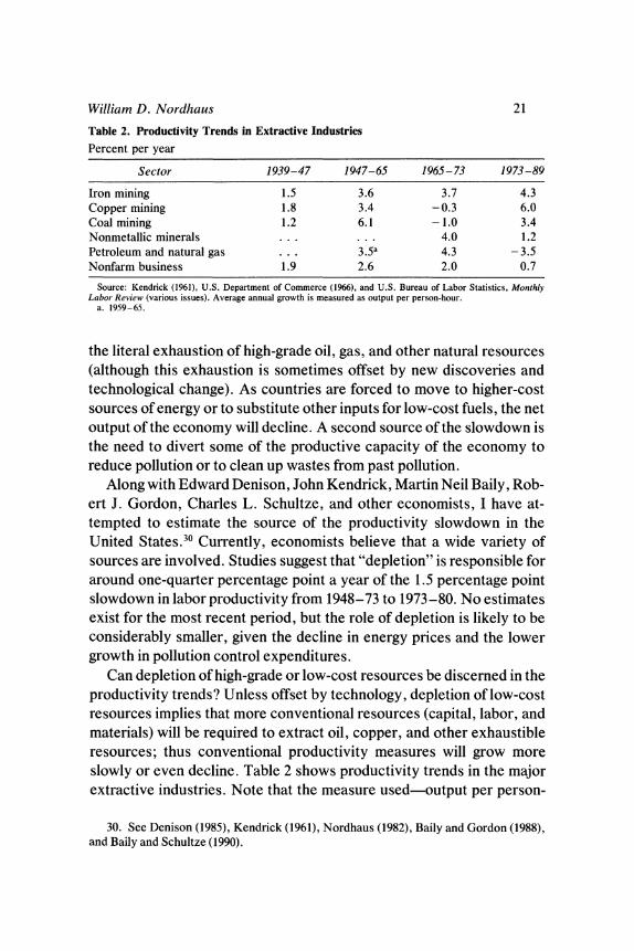
Table 2. Productivity Trends in Extractive Industries Percent per year

Sector 1939-47 1947-65 1965-73 1973-89

Iron mining 1.5 3.6 3.7 4.3 Copper mining 1.8 3.4 -0.3 6.0 Coal mining 1.2 6.1 - 1.0 3.4 Nonmetallic minerals ... ... 4.0 1.2 Petroleum and natural gas . . . 3.5a 4.3 - 3.5 Nonfarm business 1.9 2.6 2.0 0.7

Source: Kendrick (1961), U.S. Department of Commerce (1966), and U.S. Bureau of Labor Statistics, Monthly Labor Review (various issues). Average annual growth is measured as output per person-hour.

a. 1959-65.

the literal exhaustion of high-grade oil, gas, and other natural resources (although this exhaustion is sometimes offset by new discoveries and technological change). As countries are forced to move to higher-cost sources of energy or to substitute other inputs for low-cost fuels, the net output of the economy will decline. A second source of the slowdown is the need to divert some of the productive capacity of the economy to reduce pollution or to clean up wastes from past pollution.

Along with Edward Denison, John Kendrick, Martin Neil Baily, Rob- ert J. Gordon, Charles L. Schultze, and other economists, I have attempted to estimate the source of the productivity slowdown in the United States.30 Currently, economists believe that a wide variety of sources are involved. Studies suggest that "depletion" is responsible for around one-quarter percentage point a year of the 1.5 percentage point slowdown in labor productivity from 1948-73 to 1973-80. No estimates exist for the most recent period, but the role of depletion is likely to be considerably smaller, given the decline in energy prices and the lower growth in pollution control expenditures.

Can depletion of high-grade or low-cost resources be discerned in the productivity trends? Unless offset by technology, depletion of low-cost resources implies that more conventional resources (capital, labor, and materials) will be required to extract oil, copper, and other exhaustible resources; thus conventional productivity measures will grow more slowly or even decline. Table 2 shows productivity trends in the major extractive industries. Note that the measure used-output per person-

30. See Denison (1985), Kendrick (1961), Nordhaus (1982), Baily and Gordon (1988), and Baily and Schultze (1990).


hour-has major shortcomings for extractive industries because these industries are highly capital-intensive; moreover, accounting for depletion effects is a complicated procedure that has not been attempted in most productivity studies. Nonetheless, underlying trends are probably reasonably well gauged by labor productivity. The period from 1965 to 1973 showed a dismal productivity record for copper and coal mining. The period from 1973 to 1989 shows a dramatic drop in the labor productivity in crude oil and natural gas production.3' On the whole, the last decade exhibits productivity improvements in extractive industries that are above the average of the nonfarm business sector.

In summary, evidence is mixed as to whether the exhaustion of resources has contributed to the productivity slowdown in recent years. Clearly, the United States has experienced a significant slowdown in measured aggregate productivity growth in the last two decades. In extractive industries, trends for productivity have been mixed. But extractive industries are only a small fraction of total output; mining represented less than 3 percent of real GNP in 1979.32 Given the share of extractive industries and the mixed trends for productivity in those industries, I conclude that only a small fraction of the aggregate productivity slowdown can be attributed to the exhaustion of natural resources.

Long-term Trends in Resource Prices

Another way of looking at the evidence of scarcity of natural resources is to examine the long-run trends of resource prices, focusing again on market or appropriated goods. If appropriable natural resources were becoming scarcer, markets would signal this by a run-up in their relative prices. In examining prices, the most revealing trend is actually the relative movements in factor prices, rather than trends in product prices.

The impact of scarcity on prices can be illustrated by returning to the general production-function model in equation 3. Let factor rental prices

31. For petroleum and natural gas, productivity growth from 1973 to 1989 was extremely erratic, with a decline of 9.3 percent a year from 1973 to 1982, followed by a rise in labor productivity at 3.2 percent a year from 1982 to 1989. (U.S. Bureau of Labor Statis- tics, Monthly Labor Review, March 1992, p. 10).

32. Economic Report to the President, 1987 (p. 257).


be given by qi, which is the nominal price of factor i in period t, where i = L, R, T, and K. Then the factor price of resources relative to labor is given by

(13) qRqL A, L,tIf,R,,

with the analogous equation holding for land and capital services. Equation 13 tells an important story about the interplay between rela-

tive scarcity of natural resources, technological trends, and relative prices. Begin by assuming that the factor shares are constant (so that A, and Q, are constants over time). In this case, because labor is growing relative to land or other natural resources, resource and land prices should be rising relative to the price of labor. However, technological change might be resource-saving, reducing the amount of resource inputs required per unit labor at given factor prices. In this case, the share parameters might be moving sufficiently to offset the resource scarcity, thereby offsetting the tendency to increase relative resource prices.

In other words, resource and land prices will be rising relative to the price of labor, unless technological change is biased toward saving resources or land so as to offset the relative decline in those inputs. The prices of the scarce factor can only be falling relative to the abundant factor if the output elasticities are shifting in such a way as to offset the relative decline in the scarce factor. In particular, declining relative resource prices can occur if the elasticities of substitution among inputs are less than unity and technological change is resource-saving and land- saving.33

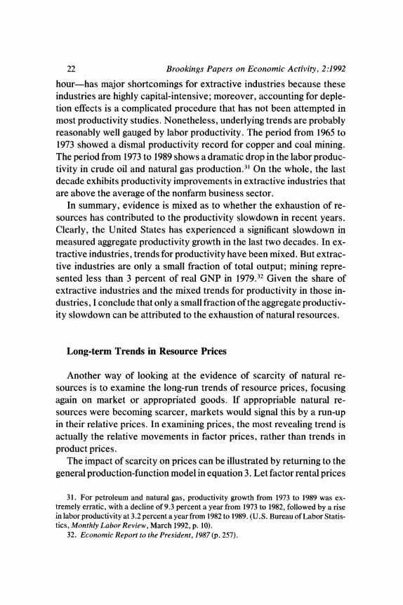
What in fact have been the trends in the prices of resources relative to the price of labor (call these the "real input prices")? Figures 2 through 6 present some of the most important examples. Figure 2 shows the prices of two key energy resources, petroleum and coal, from 1870 to 1989. The real input price of energy of these resources declined from 1880 to 1970 by a factor of between 5 and 6.5. A decline in a factor of 5

33. As an example, assume that there are two factors, labor and resources, which are combined in a constant-elasticity-of-substitution (CES) production function of the following form: Y, = F(HR R,, HL L4), where HL and HR are labor-augmenting and resource-augmenting technological change, respectively. In this specification, technological change is assumed to be purely factor-augmenting. If resource-augmenting technological change is sufficiently rapid so that HRI R, is growing faster than H,L L, even though R, is growing more slowly than L, then the price of resources will be declining relative to the price of labor.


Figure 2. Real Prices of Energy Products in the United States, 1870-1989 Real price index, 1989 = 100

Logarithmic scale 1000

< ; \ \ ~~~~~etrleumi

Coal

100

50 l I l l l l l l l I

1870 1890 1910 1930 1950 1970 1989 Source: Author's calculations based on Manthy (1978, p. 11); Statistical Abstract of the United States, 1991 (table

669, p. 408, and table 1221, p. 698); and U.S. Bureau of the Census (1975, pp. 165, 169-70). Real price is an index of the product price divided by an index of average hourly earnings in manufacturing.

over a century represents an average annual decline of 1.6 percent a year. Since 1970, however, no further decline in the real input price of the energy resources has occurred; prices increased sharply after 1973 and then declined during the 1980s.

Figure 3 shows the real input prices for four major mineral resources-copper, iron ore, lead, and zinc. The general trend in these prices has been downward during this century. Copper experienced a sharp decline until 1950, but has declined relatively little since that time. The trend in iron ore and lead looks much like the trend in real energy products, with a decline through 1970 but no significant further decline since then. Real zinc input prices have risen sharply since 1970. Taking the trend over the last century, real input prices of these four major minerals have fallen by between 1.6 and 2.4 percent a year.

Figure 4 shows the prices of four minor minerals-ones with a shorter period of use or less data. All four show significant declines in real input prices from their levels early in the century; the average annual decline in real input prices ranges from 1.3 to 2.9 percent a year. With the exception of molybdenum, the prices show a tendency to decline until 1970; after then, their movement has been less regular.


Figure 3. Real Prices of Major Minerals in the United States, 1870-1989 Real price index, 1989 = 100

Logarithmic scale

2000

1000

_ .-kkk---kkk ..............,.'. &/Cpe

Zinc ~ ~ ~ ~~~Led Iron Ore

100

50 1870 1890 1910 1930 1950 1970 1989

Source: Author's calculations based on Manthy (1978, p. 114); Statistical Abstract of the United States, 1991 (table 669, p. 408, table 1221, p. 698, and table 1241, p. 707); and U.S. Bureau of the Census (1975, pp. 165, 169- 70, 599, and 602-03). Real price is an index of the product price divided by an index of average hourly earnings in manufacturing.

Figure 4. Real Prices of Minor Minerals in the United States, 1920-89 Real price index, 1989 = 100

Logarithmic scale

1000

Aluminum

- ~~~~~~~Phosphorus

_ .....

~~~~~~~Molybdenum

100

50 _ E I I I l l 1920 1940 1960 1980 1989

Source: Author's calculations based on Manthy (1978, pp. 114 and 124); Statistical Abstract of the United States, 1991 (table 669, p. 408, table 1217, p. 696, and table 1252, p. 710); and U.S. Bureau of the Census (1975, pp. 165, 169-70, and 605). Real price is an index of the product price divided by an index of average hourly earnings in manufacturing. For 1980, molybdenum and phosphorus data points were interpolated.


Figure 5. Real Prices of Other Resources in the United States, 1870-1989

Real price index, 1989 = 100

Logarithmic scale

5000

_ , ~~~Silver

1000

1 00 -a

1870 1890 i / Stumpage l

1870 1890 1910 1930 1950 1970 1989

Source: Author's calculations based on Statistical Abstract of the United States, 1991 (table 669, p. 408, table 1188, p. 680, and table 1221, p. 698); U.S. Bureau of the Census (1975, pp. 165, 169-70, 547, and 606); and Lindhert (1988, table 1, pp. 49-51). Real price is an index of the product price divided by an index of average hourly earnings in manufacturing.

Figure 5 shows the trends in three other important resources. Silver prices reflect trends in precious metals. It is probably a better index of resource scarcity than gold, which has been pegged by governments and has contained fetishistic value over the ages (although both of these in- fluences have recently declined in importance). Real silver input prices have been highly volatile but-with the exception of the bubble during the 1980s when the Hunt brothers tried to corner the silver market- have shown no trend since 1940.

The two other prices in figure 5 contain the major surprises in the data. The first is the price of land-Lindert's series on the price of U.S. farmland-which is a good proxy for the price of undeveloped land. This series is the only one that appears to remove the influence of structures in a satisfactory manner.34 Contrary to folk wisdom,35 relative farmland

34. Lindert (1988). 35. In particular, a saying of Will Rogers comes to mind: "Land is a good investment;

they ain't making it no more."


Figure 6. Alternative Measures of Real Farmland Prices in the United States, 1860-1986 Real price index, 1986 = 100

Logarithmic scale 500

Current price .................................. .-.........-.--...Lindert series

100 1986 weights 1860 weight

50 I 1860 1870 1910 1986

Source: Author's calculations based on Lindert (1988, table 1, pp. 49-51) and U.S. Bureau of the Census (various years; 1975, pp. 165, 169-70). Real price is an index of the farmland price divided by an index of the wage rate.

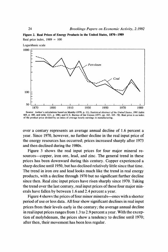
prices have actually declined over the last century, with an average decline since 1890 of 0.8 percent a year. The decline ceased after 1940. Since that time the real input price of land has increased modestly.

Because the trend in land prices runs so counter to folk wisdom, I examined farmland prices for different years. I calculated the prices by state for 1860, 1870, 1910, and 1986 and constructed fixed-weight indexes using early weights (from 1860), late weights (from 1986), and current weights. Figure 6 shows the results and a comparison with the Lind- ert price data. Not surprisingly, the 1986-weighted index rises much more quickly than the current-weight index, so the land-labor price ratio falls more slowly. However, even with this correction, land prices fall relative to wages for every index since 1860.

The other surprise is the price of "stumpage," which is the price of standing timber. It appears that stumpage prices have actually risen sig- nificantly over this century. From 1910 to 1986, the real input price of stumpage has risen by 1.5 percent a year. Most of the rise has occurred since 1970.36

What overall conclusions can be drawn from these data on long-term

36. The data on land and stumpage prices suffer from measurement problems that are much more severe than those for the other resources. These two inputs are highly hetero- genous and intrinsically immobile. Few serious index-number problems arise in creating a price index for silver, which has a conventional purity standard and low transportation costs. By contrast, the data for land and stumpage are incomplete, particularly for the earlier years; cover only part of the nation; and are estimates, rather than transaction prices.


price trends? First, the data indicate that over the last century, from an economic point of view, resources have become less scarce than labor. With the exception of stumpage, all resource prices have shown a significant drop in real prices over this century. Second, a break in this trend seems to have occurred around 1970. With the exception of copper and molybdenum, all real resource prices have either been either stable or rising since 1970. Third, a generalized increase in the relative scarcity of resources does not seem to have occurred to date. Over the last two decades, sharp increases in real input prices occurred only for zinc and stumpage. Fourth, in the most recent decade, from 1980 to 1989, the relative prices of resources have actually declined, with real prices falling for all resources except zinc and phosphorus. However, the last decade is probably heavily influenced by cyclical conditions and should not be weighted too heavily.

In short, the data on real input resource prices do not indicate that major appropriable resources have taken a major turn toward scarcity during the last century.

Direct Studies of the Drag on Economic Growth

The studies of the last two sections are backward-looking. They im- ply that resources have been but a small drag on growth to date and that technological change has overwhelmed the small drag. But what about the future? Is the power of exponential growth of population, energy use, and pollution leading humanity into an inevitable rendezvous with catastrophe?

Projecting future trends and the potential future drag from resources is qualitatively different from assessing past growth trends. We do not know the evolution of the economy; we must construct economic and scientific models of poorly understood phenomena; and we may well overlook the ultimate threats (a plague of viruses or a collision with an enormous meteorite?) as we debate other concerns, such as greenhouse warming or species depletion.

At the same time, serious research efforts have been undertaken to project future developments; these studies can form the basis for an estimate of the future drag on growth from resources. More specifically, analysts have conducted a number of sectoral studies of growth limits. The


major areas of study are energy and entropy, nonfuel minerals, land, air and water pollution, and the greenhouse effect. I will briefly sketch the results of these studies.

Before I discuss the measurements, a word is in order about the definition of output that I use below. In principle, national output should be measured as true national income, TNI, which is real national output, including appropriately measured consumption, plus the value of net ac- cumulations or decumulations of all capital. In all cases, consumption and capital accumulation are defined as the relevant flows valued with the appropriate social shadow prices; moreover, the capital flows should include physical, human, technical, research, and environmental capital. Under certain very restrictive conditions, this definition of TNI corresponds to an appropriate measure of economic welfare. The literature on new approaches to measuring true national income is burgeoning; however, stating the definition is sufficient for the purpose at hand. It is important to recognize, however, that evaluating TNI is relatively straightforward for appropriable goods and services where market prices reflect appropriate social valuations. By contrast, for inappropriable goods and services (or more accurately, for inappropriated goods or ones with incomplete property rights), market prices do not accurately reflect social valuations, and most of the difficulty is to decide on an appropriate valuation.

The methodology of estimating the drag on economic growth is to compare the impact on true national income in a "limited" case in which resources are constrained with an "unlimited" case in which resources are superabundant (but not free).37 The "growth drag" is then the difference between the unlimited and the limited cases. The growth drag may arise because either appropriable or inappropriable inputs are limited in supply. For example, resources of low-cost oil, high-grade copper, clean air or water, or pristine recreational sites may be limited. As the economy grows, these limited resources become more scarce and the

37. The counterfactual assumption that is made in the "unlimited" case is that resources are superabundant, but not necessarily free at the existing price level of resources. Consider the case of water. Say that water for irrigation currently costs $100 an acre foot, but the supply curve for water is rising sharply because of the need to go further or deeper to find more water. The counterfactual or unlimited case would arise if a new technology were discovered that could deliver desalinized water from the ocean at a cost equal to $100 an acre foot. The supply curve in the unlimited case would then be horizontal at the current price, reflecting the fact that water would be superabundant at a price of $100 an acre foot.


cost of producing the same level of satisfaction increases (or, equiva- lently, the output per bundled unit of labor and capital decreases).

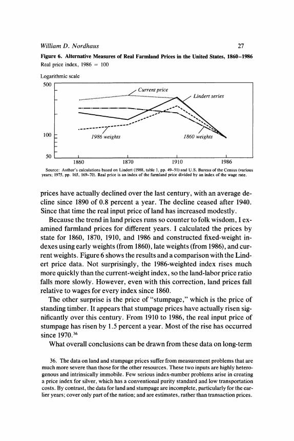
The drag on growth can be incorporated into the aggregate production function model that I introduced earlier. Assume that output is produced by a number of inputs. The impact of resource scarcity can be estimated to a first approximation by calculating the impact of a particular scarcity on the rate of growth of real income. The procedure can be seen by the following. Assume that F(R,, A, t) is the gross output that can be produced with the services of scarce land, mineral and environmental resources, Rt, and their substitutes, At. The time variable, t, in the production function represents the impacts of changing exogenous forces such as capital, labor, and technology. The cost of extracting and deliv- ering the resource services is C(Rt, At, t). Net output in the limits case, yL, is therefore

(14) YL(Rt, At, t) = F(Rt, At, t) - C(R, At, t).

For the unlimited case, assume that resources are superabundant at today's prices; write this symbolically as R-, indicating that all resources are superabundant at today's prices and grades. (Note that this applies to land and environmental resources, as well as depletable natural resources.) This implies that net output in the unlimited case in which resources are superabundant, Yu, can be written as

(15) YU(R-, At, t) = F(Roc, At,

t) - C(RO, At, t).

The difference between equation 14 and equation 15 is that in equation 15, resources do not become scarcer and more expensive, while in equation 14, the market price of the limited resource rises because of growing scarcity. Finally, the drag on growth from resources is the difference between equations 14 and 15, the levels of true national income in the unlimited and limited cases:

(16) Dragt = YU(RO, At, t) - YL(Rt, At, t).

In the estimates that follow, I will examine the drag to economic growth from 1980 to 2050.

Market Goods

"Market goods" are goods for which the social costs and benefits are captured in market transaction-that is, those without significant exter-


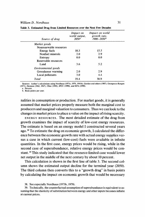
Table 3. Estimated Drag from Limited Resources over the Next Few Decades

Impact on Impact on world world output, growth rate,

Source of drag 2050a 1980-2050b

Market goods Nonrenewable resources

Energy fuels 10.3 15.5 Nonfuel minerals 2.0 2.9 Entropy 0.0 0.0

Renewable resources Land 3.6 5.2

Environmental goods Greenhouse warming 2.0 2.9 Local pollutants 3.0 4.4

Total 19.4 30.9

Sources: Author's calculations using Nordhaus (1973a, 1979, 1991b), Gordon and others (1987), Georgescu-Roegen (1971), Denison (1962, 1967), Cline (1992), IPCC (1990), and EPA (1990).

a. Percent. b. Basis points per year.

nalities in consumption or production. For market goods, it is generally assumed that market prices properly measure both the marginal cost to producers and marginal valuation to consumers. Thus we can look to the changes in market prices to place a value on the impact of rising scarcity.

ENERGY RESOURCES. The most detailed estimate of the drag from growth examines the impact of scarcity of low-cost energy resources. The estimate is based on an energy model I constructed several years ago.38 To estimate the drag on economic growth, I calculated the difference between the economic growth rate with actual energy supplies versus a case in which current (low-cost) fuels were available in infinite quantities. In the first case, energy prices would be rising, while in the second case of superabundance, relative energy prices would be constant.39 This study indicated that the resource-limited case would lower net output in the middle of the next century by about 10 percent.

This calculation is shown in the first line of table 3. The second column shows the estimated output decline for the terminal year (2050). The third column then converts this to a "growth drag" in basis points by calculating the impact on economic growth that would be necessary

38. See especially Nordhaus (1973b, 1979). 39. Technically, the counterfactual assumption of superabundance is equivalent to as-

suming that the elasticity of substitution between energy and other inputs becomes infinite at current prices.


to reduce terminal output by the amount in the second column. For energy fuels, which is the largest single figure in the table, the figure is 0. 155 percent a year on the growth rate (or 15.5 basis points a year).

NONFUEL MINERALS. In a study with a number of my colleagues, we applied the same basic methodology as just described for energy to nonfuel minerals; we used copper as a detailed case study.40 Our study derived detailed estimates of the resources and technologies for deliv- ering "copper services." Based on this model, we estimated the impact on output that would take place if the current estimates of copper availability were replaced by a hypothetical discovery of an infinite source of copper available at 1980 prices. The difference between the actual and the hypothetical supplies would constitute the growth drag. This study found that the difference between the superabundant supply and current supply estimates would produce a slowdown in growth of about one basis point a year for copper; by extending this methodology to other resource-limited nonfuel minerals, we calculated an additional slowdown of around two basis points a year.

ENTROPY. One of the hardy perennials in the ecological worry gar- den concerns the thermodynamic implications of economic activity. The most thorough treatment was a treatise in which Nicholas Georg- escu-Roegen argued that limitations of low-entropy resources will ultimately bring down the curtain on human civilization.4' "Entropy" is a technical term from thermodynamics that measures the unavailable energy of a closed system.42 For example, by extracting and burning coal, the economy is taking available energy, dissipating it into an unavailable source (ambient heat), and thereby increasing entropy. The term "negentropy" (attributed to the physicist E. Schroedinger) can be used to designate the total energy available in a system. According to Georg- escu-Roegen: [O]ur whole economic life feeds on low entropy, to wit, cloth, lumber, china, copper, etc., all of which are highly ordered [i.e., negentropic] structures.... Even with a constant population and a constant flow per capita of mined resources, mankind's dowry will ultimately be exhausted if the career of the human species is not brought to an end earlier by other factors.43

40. Gordon and others (1987). 41. Georgescu-Roegen (1971). 42. The basic principles of entropy can be found in a physics textbook such as the one

by Ohanian (1989). 43. Georgescu-Roegen (1971, pp. 277, 296). Emphasis in original.


Georgescu-Roegen's gloomy conclusion is that we must spread the jam of negentropy as thinly as possible on our meager bread: If we abstract from other causes that may knell the death bell of human species, it is clear that natural resources represent the limitative factor as concerns the life span of that species. . . And everything man has done during the last two hundred years or so puts him in the position of a fantastic spendthrift. There can be no doubt about it: any use of the natural resources for the satisfaction of non- vital needs means a smaller quantity of life in the future. If we understand well the problem, the best use of our iron resources is to produce plows or harrows as they are needed, not Rolls Royces, not even agricultural tractors.44

The Georgescu-Roegen system can be represented with the following modification of the model developed earlier. Output is given by the following production function:

(17) Y, = min[F(L,, Rt, Tt, K,; He), NOt],

where Ot is the irreducible human consumption of negentropy, q is the fixed negentropy consumption-output ratio, and other variables are as previously defined. Equation 17 asserts that increasing entropy (con- suming negentropy) in the productive process is an essential attribute of economic activity. The balance equation for negentropy is as follows: let N, be the initial stock of negentropy, with a net inflow (negentropy income) of I, from solar energy, minus dissipation and human consumption of 0t times a waste factor of Ot.4i The entropic balance equation is then

(18) Nt = Nt- I + It - otOt

The second law of thermodynamics holds that for a closed system, negentropy as measured by Nt must be running down.

How should our estimate of growth limitations account for entropy? In an economy without externalities, no correction is necessary because the entropy constraint in equation 18 is already included in the economy's technological constraints for diverse extraction and conversion activities (just as, for that matter, is the law of conservation of angular momentum, Newton's second law, Boyle's Law, or Einstein's formula on mass and energy). Equation 18 is simply redundant. It places no addi-

44. Georgescu-Roegen (1971, p. 21). 45. The amount of negentropic waste in today's economy is prodigious. Flying the au-

thor from Washington, D.C., to New Haven performs approximately (2.8 x 103) joules of irreducible work, while expending (2.4 x 108) joules of jet fuel per passenger.


tional constraints upon economic activity, and the negentropy balance equation therefore has a zero shadow price in our generalized growth model. Put differently, because virtually all the stock of negentropy is contained in appropriable energy resources, the growth drag from entropy is already contained in the growth drag from energy resources. Any further correction would be double counting.46

In addition, as Georgescu-Roegen himself argued, the flow of negentropy income is enormous relative to either depletable stocks or current use. Georgescu-Roegen writes, "For, as surprising as it may seem, the entire stock of natural resources is not worth more than a few days of sunlight!"47 It is appropriate to conclude that, as long as the sun shines brightly on our fair planet, the appropriate estimate for the drag from increasing entropy is zero.

LAND. No detailed study has been performed for agricultural land, but estimates have been made by Denison and these can be extended to future periods.48 Denison's estimate for land follows the simplified methodology outlined in equation 7. Basically, the growth drag is represented by the product of the factor share of land times the growth of the economy. For the period 1929 to 1957, Denison estimates that constraints on land slowed economic growth by five basis points a year in the United States; estimates are similar for Western Europe for the postwar period.49 I used Denison's methodology and extended it for the period 1970 to 2050. This provides an estimate of five basis points for the period covered here.

Environmental Goods

"Environmental goods" designate goods for which the social costs and benefits are not captured in market transaction, or those with significant externalities in consumption or production. An example is clean water in the lower Rhine river as it flows through the Netherlands. In the

46. Concerns might arise about the cost from inappropriable entropy, as for example, the losses to thermal efficiency from a warmer ocean.

47. Georgescu-Roegen (1971, p. 21). Note that even though our potential negentropic income is vast, we are utilizing very little of it in practice. Moreover, we are using virtually none of it to build up stocks of negentropic wealth to replace our declining stocks of valu- able fossil fuels.

48. See Denison (1962, 1967). 49. Denison (1962, p. 92).


lower Rhine, boaters, swimmers, and drinkers are not charged for their enjoyment of clean water; nor are Belgians, Germans, or French up- stream charged when they discharge untreated wastes into the upper Rhine. For environmental goods, particularly those that are unregu- lated, the commodity is not bought or sold in complete markets, so we cannot generally assume that market prices properly measure social valuation. This implies that policymakers face a difficult task in regulating, or perhaps even creating, markets; it also means that the measurement of the growth drag is much more difficult for the analysis of environmental goods.

In essence, the issue is whether to take the "cost" approach or the "utility" approach. The cost approach asks how much it would cost to prevent degradation of environmental variables. The utility approach is concerned with the actual losses or damages suffered by society. For market goods, these two approaches coincide at the margin; for imper- fectly regulated environmental goods, they do not. In the estimates that follow, I took a mixed approach.

GREENHOUSE WARMING. A number of studies investigate the impact of greenhouse warming. The impacts of warming that have been identified appear quite small relative to overall national output over the period under consideration, while the costs of control programs could be quite substantial. However, work in this area is in its infancy. Thus the calculations that follow are very tentative.

For purposes of evaluation, assume that a doubling of CO2 or its equivalent will occur by the middle of the next century. This estimate is consistent with the high projection of the scientific assessment performed by the Intergovernmental Panel on Climate Change;50 by comparison, atmospheric concentrations of CO2 have risen about 26 percent since the mid-1800s.51 Current scientific evidence suggests that a doubling of CO2 or its equivalent will lead to an equilibrium increase in global mean temperatures of 1 to 5 degrees Centigrade.52 Putting these estimates together, a rough guess is that, for the United States and other high-income countries, the cost of greenhouse warming in the middle of the next century (or of policies to slow greenhouse warming) would be in the range of 0 to 2 percent of world income (with the best guess in the

50. See IPCC (1990). 51. IPCC (1990, p. xix). 52. IPCC (1990, p. 138).


middle of this range).53 On the other hand, proposals to arrest significant future greenhouse warming are estimated to cost between 1 and 5 percent of world income.54 There is simply no way of improving these estimates today. I will take a value of 2 percent of total income in 2050 as a reasonable compromise.

OTHER ENVIRONMENTAL REGULATION. A final catchall category is the cost of preventing future deterioration of the environment (from sources other than global environmental concerns such as those I con- sidered in my discussion of greenhouse warming). Such costs consist primarily of measures to maintain air and water quality in the face of growing output.

Estimating the costs of pollution control poses many analytical and empirical hurdles because of the indirect nature of most control costs. A recent study has investigated control costs systematically for the United States. According to the U.S. Environmental Protection Agency (EPA), the annual cost of pollution control (current expenditures plus annualized capital costs) was 2.1 percent of GNP in 1990 and is estimated to rise to 2.6 to 2.8 percent of GNP in 2000.55 Figure 7 shows these costs graphically. No comparable estimates of the damages exist, although studies for some of the major categories (such as abatement of sulfur, nuclear wastes, and toxic wastes) generally find that the damages avoided are on the margin lower than the incremental costs. EPA has also collected data on comparable costs for major OECD countries. Ta- ble 4 shows estimated costs. (These are capital and operating expenditures, rather than the annualized costs shown in figure 7.) Based on recent trends, I use an estimate of an incremental rise in pollution control efforts of 3 percent of total output between 1980 and 2050.

Results

Table 3 collects the estimates from the different studies. I must emphasize that these figures are extremely tentative. They rely upon differ-

53. See Nordhaus (1991b) and Cline (1992). 54. Estimating the impacts of and the costs to slow greenhouse warming is a major

growth industry today. The estimate of the cost of arresting future climate change assumes that this requires a cut of 50 to 75 percent in greenhouse gas emissions. These estimates are drawn from surveys of the literature summarized in Nordhaus (1991 a) and Cline (1992, p. 184).

55. See U.S. EPA (1990, p. v).


Figure 7. Cost of Pollution Control in the United States, 1972-2000 Annualized as a percent of GNP

Percent 3.0

2.5-

2.0-

1.5-

1.0

0.5-

0.0. 1972 1987 1990 2000

Source: U.S. EPA (1990, p. v.). Estimate for the year 2000 assumes that municipal provisions of the Clean Water Act and investments in attaining the national ambient air quality standard for ozone will have been implemented.

ent models and disparate assumptions. While on the whole they represent the state of today's knowledge about the constraints on growth for high-income countries, they cannot foresee future technological developments or new problems that may arise. Most importantly, they are incomplete; they leave out a number of significant ecological problems (such as tropical deforestation, plagues, or genetic depletion) that may in the future prove significant.

Subject to these reservations, my estimate is that the six factors identified in table 3 will slow economic growth to the middle of the next century by about 31 basis points, or approximately one-third of a percentage point a year. (This estimate is surprisingly close to the back-of-the-enve- lope estimate presented in equation 9 above.) This growth rate compares with an estimated baseline growth rate, in the models underlying these estimates, of 2.6 percent a year for total output and 1.6 percent a year for per capita output. After taking account of the resource drag, total growth would decline to 2.29 percent a year, while per capita output


Table 4. Estimated Pollution Control Expenditures in Major OECD Countries, 1985 Percent of GDP

Pollution control Country expenditures

West Germany 1.52 United States 1.44 Finland 1.32 Netherlands 1.26 United Kingdom 1.25 France 0.85 Norway 0.82

Source: EPA (1990, pp. 4-8). Nonhousehold expenditures only.

growth under these estimates would slow this to 1.29 percent (129 basis points) a year.

Roughly speaking, then, I estimate that per capita output growth will slow by about one-fifth because of the resource constraints examined in table 3.

Implications for Today

One of the oldest battles in economic life involves the struggle between advances in technology and the drag to economic growth arising from population growth and resource exhaustion. For most of the nineteenth and twentieth centuries, concerns about resource exhaustion have receded as technological change has outpaced the modest degree of resource exhaustion. New seeds and chemical fertilizers have more than offset the need to move cultivation to marginal lands; advances in finding and drilling for oil have countered the need to drill deeper and in harsher climates; and modest pollution-abatement investments have allowed economic growth to continue while lowering concentrations of many toxic substances. In short, for the past two centuries, technology has been the clear victor in the race with depletion and diminishing returns.

But what about the future? As the globe becomes more congested, as economic activity crowds into regions that are less well endowed with natural resources, as natural ecosystems become more stressed, will history repeat itself? Or have we reached an inflection point that will lead to a turning point?


I have repeatedly emphasized that our estimates are crude, the models are primitive, the future is uncertain, and our ignorance is vast. But it is hardly interesting to say we don't know, so I will hazard the guess that resource constraints are likely to be a small but noticeable im- pediment to economic growth over the next few decades in advanced industrial countries-although an obstacle that will continue to be sur- mounted by technological advance. On the basis of current knowledge about identified economic, geological, and environmental factors, I estimate that the resource slowdown will be on the order of one-third of one percentage point a year between now and the middle of the next century. This compares with an estimated growth of output per capita of around 1.5 percent a year over the last century in advanced industrial countries. It would take either a massive slowdown in productivity growth or a massive underestimate of the constraints to growth before the resource constraints would actually produce a decline in global living standards.

Having concluded tentatively that the environmental and resource constraints on economic growth should be only modest over the next half century, it is appropriate to inquire into the implications of this finding for the conduct of government policy. The most profound implication is for our world view. Do we take the "cowboy" view or the "Dutch" view of the world? In the cowboy view, we can look forward to limitless expansion, with endless rangeland to graze, offshore waters to drill, and deserts on which to build airports, shopping centers, and parking lots. At the other extreme is a dour philosophy of limits and perils, where land must be wrested from the sea and we must be ever vigilant lest the dikes break and we become inundated by the threatening seas.

In the last three decades the environmental revolution has fundamen- tally changed our world view so that we can no longer assume that our planet will remain unaffected by human activities; the Dutch are becoming gloomier and even the cowboys are occasionally concerned. At this point, we cannot say whether the Dutch or cowboy view is the right one; whether human interventions will lead to innocuous, noticeable, serious, or catastrophic consequences. Which problems fall into which of these four categories is one of the major issues for science policy for the foreseeable future, and we cannot make intelligent choices without better scientific understanding about the interactions between human activities and resource constraints.


In addition to improving our knowledge, governments must decide where and how to intervene. In some areas, governments should intervene, while in others, governments should get out of the way of markets. An example of ineffective regulation is in the area of appropriable natural resources involving oil, natural gas, and farming. For these resources, governments the world over have probably slowed economic growth through excessive regulation of price and quantity. In the United States, oil and gas price controls have been applied and removed numerous times since 1954; these have tended to subsidize consumption and reduce production, with few redeeming social virtues. In centrally planned and developing countries, subsidies to energy production have often been extremely distortionary; the most egregious example today occurs in Russia, where oil in the summer of 1992 sold for about 10 to 20 percent of the world market price.56 Allowing energy prices to move toward the undistorted market will often be painful and lead to unwel- come shifts in the distribution of income, but in the long run, government's bowing out of the pricing and allocation process for appropriable natural resources is probably the most secure way to ensure that our limited supplies of appropriable nonrenewable and renewable resources are efficiently employed.

Efficiently managing environmental resources poses completely different issues because it requires replacing the invisible hand of markets with the visible hand of government. There are no simple approaches to setting environmental policies wisely. Governments face thorny choices in four distinct areas: selecting the appropriate areas for intervention, finding the right level of intervention, choosing the most efficient tools for minimizing the net economic harm from externalities, and coordi- nating policies where international spillovers occur. Because governments operate as monopolists in the industry of regulating environmental protection, there is no market test to apply to any of these four choices. Governments can make many sound or foolish decisions about regulating externalities without bankrupting the country or being driven from office. In some cases, such as overregulating the chemical acrylo- nitrile, the political and economic effects of excessively zealous regulation are trifling; in others, such as regulating the health and safety of

56. Lipton and Sachs (1992).


nuclear power plants, an industry can be posted unceremoniously to its grave.

Take greenhouse warming as an example of regulatory choices. Gov- ernments must decide whether greenhouse warming is sufficiently serious to warrant the setup costs of establishing a new regulatory mechanism; the Bush administration argued that doing so is premature, while many other governments have made commitments or even imposed "carbon taxes," which tax emissions of greenhouse gases like CO2. Finding the right level of intervention has proven extremely elusive, even among those who argue for taking steps to slow climate change. A good measure of the stringency of global-warming policies is the level of carbon taxes. The European Community (EC) has proposed a carbon tax of around $100 per ton carbon (which would more than triple the price of coal in the United States); by contrast, my studies suggest that a carbon tax of $5 to $10 per ton carbon is the maximum that would be justified by a cost-benefit comparison, and the $100 carbon tax would be much worse than nothing.

The third design issue in this area is the selection of policy instruments. In the United States, command-and-control approaches have been the major tools for accomplishing our regulatory objectives. As noted above, U.S. regulations have tended to be between modestly and enormously cost-ineffective, and only recently and rarely have market instruments been employed (although recognition is increasing in the policy community of the importance of cost-effective instruments). The use of taxes on ozone-depleting chemicals, the experiment with tradable SO2 permits, and the EC's contemplation of carbon taxes are hopeful signs of a trend toward using more efficient regulatory tools.

Fourth, combating greenhouse warming will require international policy coordination in much the same way as in the areas of international trade policies or exchange-rate mechanisms. While some deplore the snail's pace in reaching international agreements in global warming, a more cautious view would recall the fate of the first eleven international sanitary conventions, the League of Nations, the Treaty of Versailles, the interwar disarmament treaties, the Bretton Woods accord, SALT II, or the European Exchange Rate Mechanism and suggest that a slow movement toward consensus may be preferable to a questionable, fragile, and ambitious agreement crammed down the throats of reluctant leg-


islators and voters.57 All these difficulties should not drive us to a conclusion in the style of President Bush's former White House Chief of Staff John Sununu that nothing is better than anything. However, the difficulties should forewarn us that many policies are worse than mo- mentary hesitation.

A final-and the most intractable-issue concerns uncertainty about future resources, environmental concerns, and technology. Faced with our profound ignorance, should we respond like the Bush administration on the environment, waiting until uncertainties are resolved before act- ing, or like the Reagan administration on defense, pursuing spending programs because of uncertainties about the future? Should we assume the worst case on climate change and species loss as we did traditionally with ballistic missiles and the flashpoint on the West German border, the Fulda Gap?

The answer to these questions is no, no, and no. An appropriate approach to uncertainty is to weigh the consequences and likelihoods of a range of potential outcomes and to take actions that would maximize the expected net benefits of policies. To wait for uncertainties to be resolved may involve forgoing inexpensive steps that will prove highly beneficial if the dice roll unfavorably; to wait until uncertainties are resolved is likely to mean waiting forever; to defend against the worst case will quickly bankrupt any imaginative government. In practice, in games against nature, a best-guess strategy is likely to come tolerably close to an optimal policy. The exceptions are when the stakes are very large, the outcomes are highly asymmetrical, the processes are irreversible, or learning takes place over time.

While the appropriate treatment of uncertainty is not a controversial theoretical issue, it often poses daunting problems of estimation and im- plementation. The sheer complexity of decisionmaking under uncertainty will overwhelm most analysts, for the already-complex issues (surrounding, say, greenhouse warming or species depletion) are further complicated by the branching of probability, learning, and decision trees. Data problems are compounded because those trees depend on subjective probabilities, future values, and evolving technologies that cannot be found in any handbook of economics or physics. For imple-

57. The perils of the Treaty of Versailles were foreseen in Keynes (1920), while a history of international agreements in public health is contained in Cooper (1989).


mentation, these problems are further exacerbated by the four intrinsic difficulties I mentioned above that plague the setting of efficient environmental policies.

All these somber thoughts should not lead to despair. Rather, they emphasize the importance of careful scientific and policy analysis and establishing or strengthening institutions that contain incentives that are compatible with the thoughtful balancing of long-run costs and benefits of social investments. If it is correct, as this study suggests, that an efficiently managed economy need not fear shipwreck on the reefs of resource exhaustion or environmental collapse, this places the responsi- bility for wisely steering our economy in our own hands. The peril lies not in the stars but in ourselves.

Comments and Discussion

Robert N. Stavins: Because William Nordhaus' paper addresses indicators of changing relative scarcity, it may be of interest to note that I purchased my copy of Beyond the Limits about one month after Nord- haus purchased his, but I was not charged $20 like he was, but $10. In keeping with this observation, my comments on Nordhaus' effective critique of Beyond the Limits are from a microeconomic perspective.

The Nordhaus paper provides better guidance to the questions of concern about scarce resources than either Beyond the Limits or its bestselling predecessor, The Limits to Growth, and Nordhaus does so with less than 5 percent as many words. Having noted this, what is there left for me to add? Because I agree with the criticisms that Nordhaus makes of the Limits I and II models, I asked myself if any exceptions, any special cases, existed in which the broad claim of the Limits analysis-"overshoot and collapse"-might actually make sense.

One of the central predictions of the Limits studies is increasing scarcity of natural resources, both nonrenewable and renewable. Indeed, the Limits books originally predicted that numerous mineral and fossil fuel resources would be exhausted, leading to precipitous collapse of the economic system. In venturing this prediction, the Limits authors gave little attention, as Nordhaus notes, to the crucial roles played by exploration and discovery, technological progress, and substitution. For the authors of the Limits studies, there is no smooth transition, no gradual slowing-down of activity associated with shifting from one resource base to another. Of course, this flies in the face of the economic theory of natural resources; more importantly, it flies in the face of experience.

What, then, is the source of the Limits modelers' predictions of increasing scarcity, of approaching exhaustion? First, it is well known that the "static reserve index"-simply dividing current reserves of some

44


nonrenewable natural resource by current annual use rates-is quite useless as a measure of scarcity. It ignores the responsiveness of both the reserve stock and the use rate to price changes. Hence, the static reserve index underestimates by a dramatic margin the "time until exhaustion." In fact, these indexes have been relatively constant or increasing over time.

If we check today to see how the Limits Ipredictions have turned out, we learn that (according to their estimates) gold, silver, mercury, zinc, and lead should be thoroughly exhausted, with natural gas running out within the next eight years. Of course, this has not happened. Reserves have increased, demand has changed, substitution has occurred, and recycling has been stimulated.

There is abundant evidence, as the Nordhaus paper illustrates, that the "economic scarcity" of natural resources has been-to a large degree-declining, not increasing. Evidence goes back to the pioneering 1963 study by Harold Barnett and Chandler Morse, which found declining real unit costs of extraction over time for nonrenewable resources. ' On the other hand, more recent evidence indicates that the time trend is not monotonic, particularly in terms of relative prices. Indeed, some of the more recent analyses have detected evidence of increasing scarcity.2

It is interesting to recall, in this regard, Robert Pindyck's work, which demonstrated in theoretical terms why resource prices were likely to decline during an initial period but increase later, as the marginal product of exploration begins to decline and as technologies of recovery begin to exhibit diminishing returns.3 Margaret Slade later examined the tempo- ral price paths of numerous resource categories and verified for many resources the U-shaped pattern predicted implicitly by Pindyck's analysis.4

Research with other scarcity indicators-including marginal discovery cost' and marginal extraction cost6-has confirmed these patterns. Of course, as Richard Norgaard has argued, economic scarcity measures are accurate indicators of scarcity only if the information upon

1. Barnett and Morse (1963). 2. See, in particular, Smith (1980). 3. Pindyck (1978). 4. Slade (1982). 5. Devarajan and Fisher (1982). 6. Barnett and Morse (1963); Johnson, Bell, and Bennett (1980).


which the market is exercising its judgment is itself reasonably accurate.7 In any event, what is most striking about all of this research is that it is the renewables, not the nonrenewables, that seem most prominently to exhibit increasing scarcity (including forestry, agriculture, and fisheries).

This brings me to a case in which the Limits prophecy of "overshoot and collapse" can make sense. It is with a subset of renewable resources: biological ones, such as species. The natural growth functions of a substantial number of species exhibit what has come to be known as "critical depensation."8 This refers to a growth path (plotting the time rate of change of the stock, or population, against the stock level) in which below some critical level of the stock of the species, the natural rate of growth is negative. The result is a set of three equilibria. Two are stable: extinction (the origin) and the "carrying capacity"-the maximum stock that habitat can support. The third equilibrium is the critical one: the minimum viable population. It reflects the reality that the large ranges of habitat that exist for some species, such as whales, mean that relatively small numbers are insufficient for mating pairs to yield birth rates that exceed the rate of loss to predators and disease. This is an un- stable equilibrium.

In the nineteenth century, hunters did not shoot down each and every passenger pigeon, but nevertheless, the species was driven to extinction. A similar pattern has doomed other species. A contemporary case in point is the blue whale. Harvesting has been prohibited under international agreements since 1965, but stocks continue to decline toward extinction. Thus the case in which some kind of "overshoot and collapse" might actually occur is the case of renewable-in particular, biological-resources.9

The irony is that the so-called "exhaustible" resources are nothing of the kind. They are really quite inexhaustible, for the host of reasons economists have noted for at least a half century. That is why such resources are better labeled "nonrenewable resources." It is the renewable resources that in some cases are very much exhaustible-not because of their finiteness, but because of the way they are managed. The

7. Norgaard (1990). 8. Clark(1990). 9. A broader class of biological growth functions, exhibiting generalized "depensa-

tion," can result in oscillation, another of the Limits modelers' scenarios.


problem typically is not physical limits on resource availability; on the contrary, improper incentives and inadequate information are more often the source of the declining stocks. 10 Thus the reason why some resources-water, forests, fisheries, and some species of wildlife-are threatened, while others-principally minerals and fossil fuels-are not is that the scarcity of nonrenewable resources is well reflected in market prices. This is much less the case for renewable resources, which, in fact, are characterized by being open access or common property resources.

This conclusion prompts at least two responses. First, it can be said that this conclusion is not really what the Limits authors had in mind when they predicted "overshoot and collapse." This is certainly true. Second, it could be said that the necessity to identify such a special case in order to validate-in a sense-the Limits conclusions is itself evidence of the overall legitimacy of the Nordhaus critique. This is also correct.

Having said that, I wish to turn to an area that is best categorized as not even an exception to the Nordhaus critique, but as an extension of it. Something that differentiates both the time of publication and the con- tents of Limits II from Limits I is an expanded concern beyond nonrenewable and renewable resources to environmental resources, such as clean air and water. Here the empirical evidence is growing that-contrary to the assumptions of the Limits modelers-economic growth does not necessarily produce greater pollution.

For some environmental problems, such as inadequate sanitation and unsafe drinking water, there is a monotonic and inverse relationship between the level of the environmental threat and per capita income. " I This relationship holds both cross-sectionally (across nations) and for single nations over time. For other environmental problems, the relationship with income level is not monotonic at all, but a "hill." At low levels of income, pollution increases with per capita income. Then at some point, pollution begins to decline with further increases in income. This is true of most forms of air'2 and water pollution, some types of deforestation, and habitat loss.

Pollution increases from the least developed agricultural countries to

10. Tietenberg (1992). 11. World Bank (1992). 12. Grossman and Krueger (1992).


those beginning to industrialize fully, such as Mexico and the emerging market economies of Eastern Europe and parts of the former Soviet Union. After peaking in such nations, pollution declines in the wealth- ier, industrialized nations that have both the demand for cleaner air and water and the means to provide it. Finally, for another set of environmental pollutants, including carbon dioxide emissions, the relationship between per capita income and emission levels increases monotoni- cally, at least within the realm of experience.

In conclusion, I would like to acknowledge that the first Limits study did have one positive social impact. It provided the stimulus for some leading economists to carry out work in the area of natural resource depletion. I will close my commentary on Nordhaus's excellent paper by noting that the second study is following in that tradition.

The Limits analysis is particularly disappointing because the general area of inquiry-global resource and environmental issues-would benefit from more analysis. It is obviously not enough to say that markets will automatically respond appropriately to scarcity. Imperfections in markets and imperfections in public policies clearly reduce the effec- tiveness of these responses. Common property resources, externalities, the tax treatment of resources, and price controls are more thanjust rare exceptions. Unfortunately, none of the required analysis is provided by the Limits modelers.

Furthermore, the current debate surrounding the notion of "sustainability" is not advanced by the analyses of Limits I or II. This is un- fortunate because that debate has recently moved beyond an economic critique of what is, at best, a poorly defined concept, to some attention to a set of underlying and better-defined issues.'3 The result may eventually be some common ground for discussion between economists and ecologists-who typically hold such different perspectives-on key issues such as the composition of social capital, intergenerational equity, and the scale of human activity. 14

Finally, it is worthwhile to reflect briefly on the U.S. experience with pollution control policies because doing so offers the reminder that more than once-in the environmental area, as perhaps in others-society, in choosing public policies, has tended to "do the right thing," although for

13. Solow(1991). 14. Toman and Crosson (1991).


the "wrong reasons." A recent example of this is the planned cutback under the Clean Air Act amendments of 1990 of emissions of sulfur dioxide as a means of limiting acid rain. The original motivation was to pro- tect Adirondack lakes and Eastern forests, but the evidence has pointed toward very small benefits, relative to the costs of control. More recently, however, evidence has emerged indicating that the human health impacts of sulfate particles can be significant, and may indeed provide some economic rationale, after all. '5

This leads me to ask what the actual policy prescriptions of the Limits analysis are. It is not perfectly clear. The book lays out a set of "steps to avoid collapse," but some of these are impossible to translate into terms of public policy. Of those that can be translated into public policy, the first is one that is hard to disagree with, in general, anyway: "improving the signals." The Limits authors call for internalizing environmental costs in prices, presumably through taxes or tradable permit systems. In addition, and somewhat more controversially, they call for recasting economic indicators such as GNP to account for uninternalized externalities and the depreciation of natural capital.

Second, the Limits authors recommend minimizing the use of nonrenewable resources. This recommendation does not, as a general rule, make sense. The authors urge society to "recycle whenever possible," which also, of course, would be flawed public policy. Recycling has a role to play, but a limited one in extending the resource base. In terms of waste management strategies, safe landfilling and incineration should certainly be part of the overall portfolio.

Third, the Limits authors call for the prevention of "the erosion of renewable resources," urging society to maintain stocks at their current levels. Again, as a general rule, this makes no sense economically, whether for soils, water supplies, or biological species.

In a sense, I may have given the Limits modelers too much credit for these policy prescriptions because they also maintain that such "piece- meal approaches," as they call them, are doomed to failure and that only the cessation of economic growth can avoid "overshoot and collapse." Thus as Nordhaus notes, the modelers do indeed call for a cessation of economic growth. In so doing, they demonstrate a common misunderstanding among noneconomists about the nature of economic growth.

15. Portney (1990).


They seem to think of it in terms of more and more cars or refrigerators for those who already have them, not more efficient refrigerators, more CD's instead of record players, or more and better vaccines to prevent disease.

In conclusion, I would like to acknowledge that the first Limits study did have one positive social impact. It provided the stimulus for some leading economists to carry out work in the area of natural resource depletion. I will close my commentary on Nordhaus's excellent paper by noting that the second study is following in that tradition.

Martin L. Weitzman: This is an outstanding paper. William Nordhaus is the senior scholar in this area who is almost uniquely positioned to collect, dissect, and reassemble in perspective all the relevant limits-to- growth arguments. The result is an impressive, balanced account that leaves few stones unturned. I think this paper represents the economic state of the art, circa 1992, in dealing seriously and honestly with the major limits-to-growth arguments. The conclusions seem to me to be basically reasonable and well argued. As a discussant, I am left with the meager task of rearranging a few stories here or there and looking at the landscape from some slightly different angles.

I would like to address a general point about evaluating the drag on growth surrounding environmental improvement that is not fully understood or articulated in the literature. This point goes beyond the cost versus utility distinction that is frequently made.

How much is it really "costing us" to prevent local environmental deterioration such as air and water pollution? One way to get a handle on this concept is to look at a figure such as total annualized costs for all pollution control activities in the United States. The Environmental Pro- tection Agency (EPA) has recently performed a systematic study that shows pollution control costs as a fraction of GNP rising from 0.9 percent in 1972 to 1.9 percent in 1987 and projected to increase to around 2.7 percent in the year 2000.1 It is tempting to think of this percentage as representing the cost of a clean environment. Actually, there are reasons to believe that such numbers represent a systematic underestimate of "environmental drag."

Consider the following amended version of the standard one-sector

1. U.S. EPA (1990).


neoclassical growth model. A homogeneous output is produced by capital and labor with the possible help of technological progress. Suppose that the output itself is objectionable, if it is not corrected, because of environmental disamenities such as pollution, crowding, and degradation of natural sites. For a variety of reasons, this kind of environmental sensitivity increases with rising income. The degree of environmental disamenity can be lessened by expending resources to improve the environment. The homogeneous output is divided into three components. The first two components are traditional consumption and investment. The third component might be thought of as cleanup costs of pollution, but a far more general interpretation is possible: the total cost of all environmental policies.

The level of environmental amenity is now some function negatively related to economic activity (represented by total output) and positively related to the amount of national income spent on environmental improvements. That is, society can trade off some of the "bad" from economic activity by spending more on the "good" of environmental cleanup.

Now any socially efficient approach to lessening the degree of environmental disamenity as an economy develops will consist of a two- pronged attack. The direct prong is to spend more on environmental improvement. The indirect prong is to have less output by growing less fast. For instance, an efficient strategy for decreasing automobile pollution will contain some combination of controlling emissions on each auto combined with a mechanism for restraining the total number of autos.

The degree to which society goes with one approach or the other will depend, among other things, on some technologically given parameter essentially measuring the elasticity of environmental improvement with respect to spending. If this elasticity is high and the environment im- proves readily with environmental spending, then the adverse environmental consequences that accompany increased economic activity will be offset by greater environmental spending. In this case, the income spent on environmental improvement-the "cost of clean"-is a relatively good proxy for the appropriate social cost of preventing environmental deterioration.

However, when the elasticity of environmental improvement with respect to income is smaller, the socially efficient response to lessening


the impact of environmental disamenities is to rely more on lowering national product by slowing economic growth than on increasing environmental spending. This is because it is expensive to undo environmental degradation by increased spending. In this case-when the elasticity of environmental improvement with respect to environmental spending is low-the level of environmental spending underestimates the degree of environmental drag, as measured by the "equivalent evaporation" or "equivalent leakage" of national product because of the externality. I do not know the correct parameter values, but a theoretical result suggests that with elasticities of one or one-half, the appropriate drag is two or three times the spending on environmental cleanup.

A correction such as this alone would not be nearly enough to reverse the essence of Nordhaus' final accounting, but I suspect that the fraction of GNP spent on improving the environment is likely to continue to grow. Many hidden costs, such as protecting wetlands, do not show up in any EPA numbers. I suspect too that the magnitude of such invisible costs is likely to increase in the future. When all these effects are combined, the distant future impact of local environmental goods might be considerably more than has been calculated. My main point is not that the story Nordhaus is telling comes unstuck empirically, but that in principle a serious issue of undervaluing environmental drag may occur when only spending on environmental improvement is used as a proxy.

I would like now to expand upon a point that has already been made well in this paper. As Nordhaus fairly and accurately shows, the debate about future limits to growth is ultimately an empirical one. The outcome depends upon deep structural parameters and assumptions about human behavior. The cast of prominent characters is by now familiar: elasticities of substitution, factor augmenting technological change, population growth, stocks of natural resources, the income elasticity of environmental tastes, and so forth.

But all this begs a further question. If the debate about the feasibility and desirability of future economic growth will not be resolved by theoretical reasoning, but must ultimately be resolved by the answers to empirical questions, then why does such an enormous difference of opin- ions occur? In a way, the very excellence of this paper begs the question more strongly. To economists, or at least to me, the conclusions of this paper seem reasonable, even convincing. Yet the other side in the limits- to-growth debate argues ferociously that we are perilously close to an


environmental catastrophe. If Nordhaus is right that the question ultimately comes down to a difference in empirical world views, then what are the empirical differences, where do they come from, and why are they so large? I think it is important to try to address such issues, however tentatively. There may be a some value in trying to understand a little better why the advocates of the limits-to-growth view see things so differently and what, if anything, might narrow the differences.

I think that there are two major differences in empirical world views between mainstream economists and anti-growth conservationists. The average ecologist sees everywhere that carrying capacity is a genuine limit to growth. Every empirical study, formal or informal, confirms this truth. And every meaningful theoretical model has this structure built in. Whether it is algae, anchovies, or arctic foxes, a limit to growth always appears. To be sure, carrying capacity is a long-term concept. There may be temporary population upswings or even population explo- sions, but they always swing down or crash in the end because of finite limits represented by carrying capacity. And Homo sapiens is just another species-one that actually is genetically much closer to its closest sister species, chimpanzees, than most animals are to their closest sister species.

Needless to say, the average contemporary economist does not readily see any long-term carrying capacity constraints for human beings. The historical record is full of past hurdles to growth that were overcome by substitution and technological progress. The numbers on contemporary growth, and the evidence before one's eyes, do not seem to be send- ing signals that we are running out of substitution possibilities or out of inventions that enhance productivity.

This is the first major difference between the empirical big picture seen by mainstream economists and limits-to-growth conservationists. The second major difference is a little more subtle, to my mind. It concerns the possibility that humans can say at some point "enough is enough"; we have more than sufficient goods to go around and must begin seriously to limit output and consumption.

Economists are skeptical of the possibilities for such self-limiting behavior. Advocates of limits tend to be more optimistic that, in a state of general abundance, human attitudes toward further accumulation can change or be changed.

I will stop with this brief list. A huge chasm between world views on


these two issues obviously exists. Could limits-to-growth conservationists ever come closer to seeing things the economist's way? Well, perhaps they have, a little bit, over time. Perhaps papers like this one have made some difference.

What about the other direction? Could economists ever believe anything like the above two limits-to-growth arguments? Actually, economists did, once-not a decade or generation ago, but a century or so ago.

Much of classical economics, with its long-run "stationary state," had a fairly well developed limits-to-growth argument. To be sure, it lacked the drama and violent overshooting of the latest catastrophic versions, but the argument that growth would have to stop because of limiting factors-most notably land-was definitely there.

Furthermore, the writings of our esteemed colleagues of the past are full of references to the idea that society will achieve general satiation in the distant future, when even the poorest will live as the richest once had. With more than enough to go around, people will work less and en- joy leisure more. This vision is expressed in the writings of Marx, of Mill, of Keynes, and of many others.

It can be argued that these economists underestimated the potential of technical change, or that they did not really understand human nature. Maybe that is true. But I must say it gives me some pause in trying to think about the distant future. Maybe it is we who are now overesti- mating the potential of technical change or it is we who do not really understand human nature. If we mainstream economic thinkers reversed ourselves so strongly over the last century, why shouldn't we reverse ourselves again over the next century?

Nordhaus bravely takes a stand on what will happen to growth in the middle of the next century, after properly cautioning us about how uncertain we must be. A modest slowdown is what he predicts. I suppose my point estimate would be close to his, but I think my standard devia- tion might be larger.

General Discussion

The contrast between the world views of mainstream economists, as represented in this paper, and adherents of the limits-to-growth school captured the attention of several participants. Richard Cooper observed that economists themselves are implicated in the notion of limits to


growth. Classical economists such as David Ricardo made the mistake of applying the concept of diminishing marginal returns to the long run, as well as to the short run. Cooper expressed optimism that functional substitutes would be found for any good that becomes too scarce and too costly. Although not quite as optimistic, William Nordhaus agreed with Cooper and cautioned against costly overreactions by policymakers. The dangers of overreaction prompted Nordhaus to draw a parallel to Arthur Okun's statement about inflation: the problem with inflation is not the cost of inflation, but the cost of reacting to stop it.

William Brainard suggested two further distinctions between the two world views. First, environmentalists, more so than economists, tend to be concerned about irreversibility-the fear that the world is moving down a path from which there is no return. Second, environmentalists envision a future world in which each country has living standards on a par with the United States or Switzerland today. Environmentalists' concerns and strong policy prescriptions stem from envisioning the consequences of such a high standard with current patterns of pollution and resource depletion. Hence the underlying vision that motivates environmentalists differs greatly from the world as it is today, or the world that economists, implicitly, believe would evolve. Nordhaus added that there was a common misunderstanding about what economic growth en- tails. It is not a linear process in which one steel mill or one landfill leads inexorably to ten as the economy grows. He emphasized that we should be concerned about depletion of biological resources in particular, rather than renewable resources in general. The sustainability of resources that are both scarce and essential in some way should be a particular concern.

Martin Weitzman noted the controversial argument by the limits-to- growth school that "enough is enough": that we have reached satiation in consumption of goods and services. Robert Gordon questioned that claim in view of large inequalities in the distribution of goods and services around the world. Enough is enough for whom? Gordon asked. Certainly not for starving children in Somalia, or for Americans in the bottom 20 percent of the income distribution, or for 80 percent of the world's people, he argued.

Nordhaus suggested several other reasons for the difference in world views. First, the time horizons of the two schools differ: mainstream economists would be reluctant to project trends over a hundred years as


environmentalists do. Second, environmentalists weigh environmental factors heavily in their utility function, putting a heavy emphasis on environmental consumption. He acknowledged that those with a biocen- tric view would reject economists' utilitarian analysis. Some environmentalists would wish to include the "utility" of other forms of life, as well as human utility, in the societal welfare function. Third, environmentalists may attach substantial weight to the risk of damage from un- foreseen factors that cannot be fully accounted for in any projection. Nordhaus compared the mindset of an environmentalist who favors zero economic growth to that of the captain of the QE II: "You can't hit a shoal if you don't leave the port." Fear of the unknown, coupled with concern about irreversibilities, leads some environmentalists to adopt a disinclination for any growth or change, Nordhaus argued. Cooper addressed the difficulties of dealing with uncertainty. Because no markets exist to insure against the high-level risks of failure of the earth as a system, a common view on collective risk aversion is needed and can be established only through the political process, where debate will be fierce and where the prevailing view may change over time.

Robert Gordon noted that the EPA estimates of the costs of pollution control amount to a reduction of less than one-tenth of 1 percent in GDP growth rates. He judged this figure to be too low in view of the extent of environmental regulation. Nordhaus stressed the limitations of the EPA calculations. They represent only the costs shown on firms' books as in- curred in controlling pollution. This calculation is likely to understate the real total cost by omitting other parts of it, including the chilling effect that environmental controls may have in restraining certain types of research and development, and the costs of shifting from dirty processes, whose costs of controlling pollution are high, to clean processes, whose control costs are lower. On the other hand, the EPA figures may be overstated to the extent that innovation that reduces other costs is induced by the introduction of environmental controls; these induced cost reductions will not be counted, but the accounting costs of the controls will be.

Remarking on the fact that stumpage prices fail to follow the same pattern as other resources, Robert Hall suggested that the pattern arises because forests in the United States, at least in the Northwest, are largely government-owned. He suggested that large efficiency losses have arisen from underexploitation of federal forests.


References

Baily, Martin Neil, and Robert J. Gordon. 1988. "The Productivity Slowdown, Measurement Issues and the Explosion of Computer Power." BPEA, 2:1988, 347-420.

Baily, Martin Neil, and Charles L. Schultze. 1990. "The Productivity of Capital in a Period of Slower Growth." BPEA, Microeconomics, 369-406.

Barnett, Harold J., and Chandler Morse. 1963. Scarcity and Growth: The Eco- nomnics of Natural Resource Availability. Baltimore: John Hopkins Univer- sity Press.

Beckerman, Wilfred. 1972. "Economists, Scientists, and Environmental Catas- trophe." Oxford Economic Papers 24(3):327-44.

. 1992. "Economic Growth and the Environment: Whose Growth? Whose Environment?" World Development 20(4):481-96.

Clark, Colin W. 1990. Mathematical Bioeconomics: The Optimal Management of Renewable Resources. New York: John Wiley and Sons.

Cline, William R. 1992. The Economics of Global Warming. Washington: Insti- tute for International Economics.

Cooper, Richard N. 1989. "International Cooperation in Public Health." In Can Nations Agree? Washington: Brookings.

Day, Richard H. 1983. "The Emergence of Chaos from Classical Economic Growth." Quarterly Journal of Economics 98(2):201-13.

Denison, Edward. 1962. The Sources of Economic Growth in the United States and the Alternatives Before Us. New York: Committee for Economic Devel- opment.

. 1967. Why Growth Rates Differ: Postwar Experiences in Nine Western Countries. Washington: Brookings.

. 1985. Trends in American Economic Growth, 1929-1982. Washington: Brookings.

Devarajan, Shantayanan, and Anthony C. Fisher. 1982. "Exploration and Scar- city." Journal of Political Economy 90(6): 1279-90.

Forrester, Jay Wright. 1971. World Dynamics. Cambridge, Mass.: Wright- Allen Press.

Georgescu-Roegen, Nicholas. 1971. The Entropy Law and the Economic Proc- ess. Cambridge, Mass.: Harvard University Press.

Gordon, Robert, and others. 1987. Toward a New Iron Age? Cambridge, Mass.: Harvard University Press.

Grossman, Gene, and Alan Krueger. 1992. "Environmental Impacts of a North American Free Trade Agreement." In The U.S.-Mexico Free Trade Agreement, edited by Peter Garber. Cambridge, Mass.: MIT Press (forthcoming).

Intergovernmental Panel on Climate Change (IPCC). 1990. Climate Change: The IPCC Scientific Assessment. Cambridge: Cambridge University Press.

Johnson, Manuel H., Frederick W. Bell, and James T. Bennett. 1980. "Natural


Resource Scarcity: Empirical Evidence and Public Policy." Journal of Envi- ronmental Economics and Management 7 (3):256-71.

Kendrick, John. 1961. Productivity Trends in the United States. Princeton, N.J.: Princeton University Press.

Keynes, John Maynard. 1920. The Economic Consequences of the Peace. New York: Harcourt, Brace and Howe.

Kuznets, Simon. 1977. "Two Centuries of Economic Growth: Reflections on U.S. Experience." American Economic Review, Papers and Proceedings 67(1): 1-14.

Lindert, Peter H. 1988. "Long-Run Trends in American Farmland Values." Ag- ricultural History 62(3):45-85.

Lipton, David, and Jeffrey Sachs. 1992. "Prospects for Russia's Economic Re- forms." BPEA, 2:1992, 213 -65.

Maddison, Angus. 1982. Phases of Capitalist Development. Oxford: Oxford University Press.

Malthus, T. R. 1817. An Essay on the Principle of Population. London: J. Johnson.

Manthy, Robert S. 1978. Natural Resource Commodities-A Century of Statis- tics: Prices, Output, Consumption, Foreign Trade, and Employment in the United States, 1870-1973. Baltimore: Johns Hopkins University Press.

May, Robert M. 1974. "Biological Populations with Non-Overlapping Genera- tions: Stable Points, Stable Cycles, and Chaos." Science 186:645-47.

Meadows, Dennis L., and others. 1974. Dynamics of Growth in a Finite World. Cambridge, Mass.: Wright-Allen Press.

Meadows, Donella H., and others. 1972. The Limits to Growth. New York: Uni- verse Books. (Limits 1)

Meadows, Donella H., Dennis L. Meadows, and J0rgen Randers. 1992. Beyond the Limits. Post Mills, Vt.: Chelsea Green Publishing Company. (Limits II)

Nordhaus, William D. 1973a. "World Dynamics: Measurement Without Data." Economic Journal 83(December): 1156-83.

1973b. "The Allocation of Energy Resources." BPEA, 3:1973, 529-70. 1979. The Efficient Use of Energy Resources. New Haven, Conn.: Yale

University Press. . 1982. "Economic Policy in the Face of Declining Productivity Growth."

European Economic Review 18(May/June): 131-57. . 1991a. "The Costs of Slowing Climate Change: A Survey." The Energy

Journal 12(1):37-65. . 1991b. "To Slow or Not to Slow: The Economics of the Greenhouse Ef-

fect." Economic Journal 101(July):920-37. . Forthcoming. "Economic Growth on a Planet Under Siege." Weltwirt-

schaft Wissenschaft. Norgaard, Richard B. 1990. "Economic Indicators of Resource Scarcity: A Crit-

ical Essay." Journal of Environmental Economics and Management 19(1): 19-25.

Ohanian, Hans C. 1989. Physics. New York: Norton.


Pindyck, Robert S. 1978. "The Optimal Exploration and Production of Nonre- newable Resources." Journal of Political Economy 86(5):841-61.

Portney, Paul R. 1990. "Economics and the Clean Air Act." Journal of Eco- nomic Perspectives 4(4): 173-81.

Slade, Margaret E. 1982. "Trends in Natural Resource Commodity Prices: An Analysis in the Time Domain." Journal of Environmental Economics and Management 9(2): 122-37.

Smith, V. Kerry. 1980. "The Evaluation of Natural Resource Adequacy: Elu- sive Quest or Frontier of Economic Analysis?" Land Economics 56(3):257- 98.

Solow, Robert M. 1967. "Some Recent Developments in the Theory of Pro- duction." In The Theory and Empirical Analysis of Production, edited by Murray Brown. New York: Columbia University Press.

. 1974. "The Economics of Resources and the Resources of Economics." American Economic Review, Papers and Proceedings 64(2): 1-14.

. 1991. "Sustainability: An Economist's Perspective." The Eighteenth J. Seward Johnson Lecture. Woods Hole, Mass.: Marine Policy Center, Woods Hole Oceanographic Institution.

Study of Critical Environmental Problems. 1970. Man's Impact on the Global Environment: Assessment and Recommendation for Action; Report. Cam- bridge, Mass.: MIT Press.

Tietenberg, Thomas H. 1988. Environmental and Natural Resource Economics. Glenview, Ill.: Scott, Foresman and Co.

. 1992. Environmental and Natural Resource Economics. New York: Harper Collins.

Toman, Michael A., and Pierre Crosson. 1991. "Economics and 'Sustainability': Balancing Tradeoffs and Imperatives." Discussion Paper ENR-91-05. Wash- ington: Resources for the Future (January).

U.S. Bureau of the Census. 1975. Historical Statistics of the United States, Co- lonial Times to 1970. Washington: Department of Commerce.

. Various years. Census of Agriculture. Washington: Department of Commerce.

U.S. Department of Commerce. 1966. Long-term Economic Growth, 1860- 1965. Washington.

U.S. Environmental Protection Agency. 1990. Environmental Investments: The Cost of a Clean Environment; A Summary. EPA-230-12-90-084. Wash- ington: U.S. Environmental Protection Agency (December).

World Bank. 1992. World Development Report 1992. New York: Oxford Uni- versity Press.

World Commission on Environment and Development. 1987. Our Common Fu- ture. Oxford: Oxford University Press.

Lethal Model 2: The Limits to Growth Revisited · WILLIAM D. NORDHAUS Yale University Lethal Model...

Documents

Transcript of Lethal Model 2: The Limits to Growth Revisited · WILLIAM D. NORDHAUS Yale University Lethal Model...