
Let me introduce myself, I am Sébastien Lagarde and ......Let me introduce myself, I am Sébastien...
55
1
Transcript of Let me introduce myself, I am Sébastien Lagarde and ......Let me introduce myself, I am Sébastien...

1
2
#Short presentation of the guys
Let me introduce myself, I am Sébastien Lagarde and, together with my co-worker Antoine
Zanuttini, we are part of a team currently working on a PC/XBOX360/PS3 game.
For our game’s needs, we are looking to increase realism with more accurate indirect lighting.
And the primary technique to handle it in real-time today is through IBL.
I would first advise that I will restrict this talk to static glossy and specular IBL. By static I mean
not generated in real-time.
And second that I will only refer to cubemaps as parameterizations for IBL, thanks to their
hardware efficiency.
There are two main IBL usage in games: to simulate distant lighting or to simulate local
lighting.

3
4
#This slide explains distant IBL
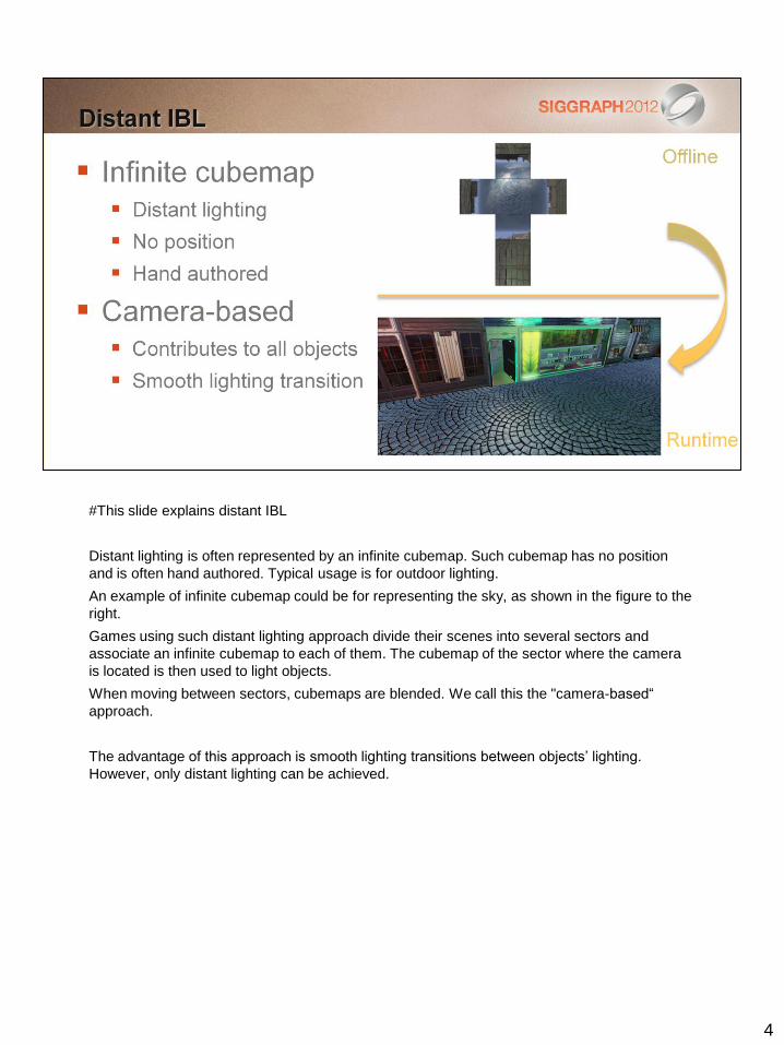
Distant lighting is often represented by an infinite cubemap. Such cubemap has no position
and is often hand authored. Typical usage is for outdoor lighting.
An example of infinite cubemap could be for representing the sky, as shown in the figure to the
right.
Games using such distant lighting approach divide their scenes into several sectors and
associate an infinite cubemap to each of them. The cubemap of the sector where the camera
is located is then used to light objects.
When moving between sectors, cubemaps are blended. We call this the "camera-based“
approach.
The advantage of this approach is smooth lighting transitions between objects’ lighting.
However, only distant lighting can be achieved.
5
#This slide explains local IBL
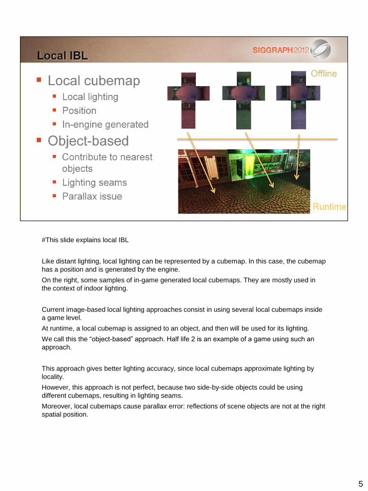
Like distant lighting, local lighting can be represented by a cubemap. In this case, the cubemap
has a position and is generated by the engine.
On the right, some samples of in-game generated local cubemaps. They are mostly used in
the context of indoor lighting.
Current image-based local lighting approaches consist in using several local cubemaps inside
a game level.
At runtime, a local cubemap is assigned to an object, and then will be used for its lighting.
We call this the “object-based” approach. Half life 2 is an example of a game using such an
approach.
This approach gives better lighting accuracy, since local cubemaps approximate lighting by
locality.
However, this approach is not perfect, because two side-by-side objects could be using
different cubemaps, resulting in lighting seams.
Moreover, local cubemaps cause parallax error: reflections of scene objects are not at the right
spatial position.
6
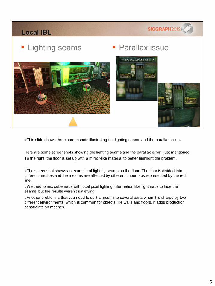
#This slide shows three screenshots illustrating the lighting seams and the parallax issue.
Here are some screenshots showing the lighting seams and the parallax error I just mentioned.
To the right, the floor is set up with a mirror-like material to better highlight the problem.
#The screenshot shows an example of lighting seams on the floor. The floor is divided into
different meshes and the meshes are affected by different cubemaps represented by the red
line.
#We tried to mix cubemaps with local pixel lighting information like lightmaps to hide the
seams, but the results weren’t satisfying.
#Another problem is that you need to split a mesh into several parts when it is shared by two
different environments, which is common for objects like walls and floors. It adds production
constraints on meshes.

7
8
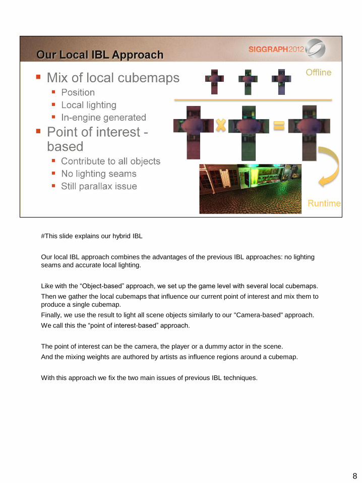
#This slide explains our hybrid IBL
Our local IBL approach combines the advantages of the previous IBL approaches: no lighting
seams and accurate local lighting.
Like with the “Object-based” approach, we set up the game level with several local cubemaps.
Then we gather the local cubemaps that influence our current point of interest and mix them to
produce a single cubemap.
Finally, we use the result to light all scene objects similarly to our "Camera-based" approach.
We call this the “point of interest-based” approach.
The point of interest can be the camera, the player or a dummy actor in the scene.
And the mixing weights are authored by artists as influence regions around a cubemap.
With this approach we fix the two main issues of previous IBL techniques.
9
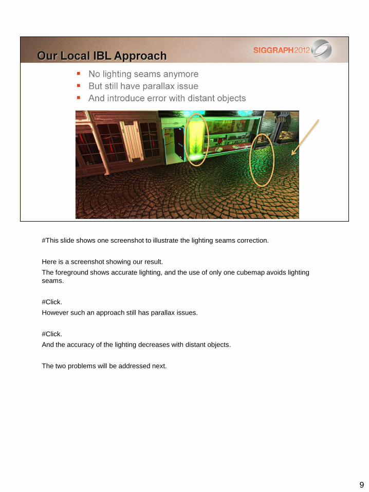
#This slide shows one screenshot to illustrate the lighting seams correction.
Here is a screenshot showing our result.
The foreground shows accurate lighting, and the use of only one cubemap avoids lighting
seams.
#Click.
However such an approach still has parallax issues.
#Click.
And the accuracy of the lighting decreases with distant objects.
The two problems will be addressed next.
10
11
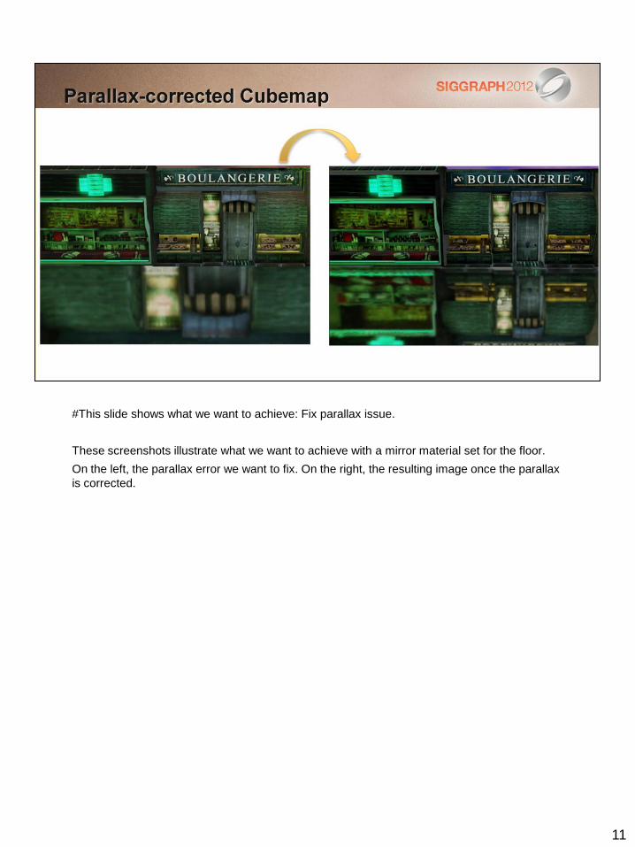
#This slide shows what we want to achieve: Fix parallax issue.
These screenshots illustrate what we want to achieve with a mirror material set for the floor.
On the left, the parallax error we want to fix. On the right, the resulting image once the parallax
is corrected.
12
#This slide introduces the standard method
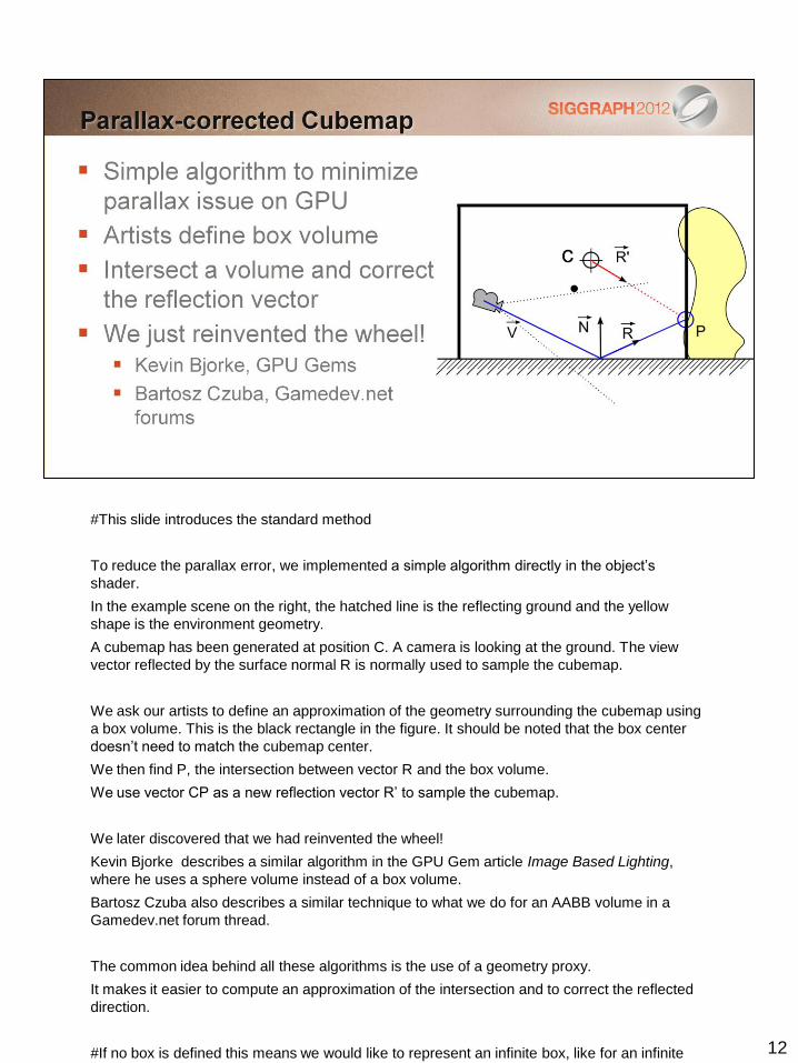
To reduce the parallax error, we implemented a simple algorithm directly in the object’s
shader.
In the example scene on the right, the hatched line is the reflecting ground and the yellow
shape is the environment geometry.
A cubemap has been generated at position C. A camera is looking at the ground. The view
vector reflected by the surface normal R is normally used to sample the cubemap.
We ask our artists to define an approximation of the geometry surrounding the cubemap using
a box volume. This is the black rectangle in the figure. It should be noted that the box center
doesn’t need to match the cubemap center.
We then find P, the intersection between vector R and the box volume.
We use vector CP as a new reflection vector R’ to sample the cubemap.
We later discovered that we had reinvented the wheel!
Kevin Bjorke describes a similar algorithm in the GPU Gem article Image Based Lighting,
where he uses a sphere volume instead of a box volume.
Bartosz Czuba also describes a similar technique to what we do for an AABB volume in a
Gamedev.net forum thread.
The common idea behind all these algorithms is the use of a geometry proxy.
It makes it easier to compute an approximation of the intersection and to correct the reflected
direction.
#If no box is defined this means we would like to represent an infinite box, like for an infinite
cubemap (sky).
13
#This slide introduces a cheaper method
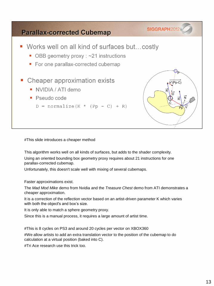
This algorithm works well on all kinds of surfaces, but adds to the shader complexity.
Using an oriented bounding box geometry proxy requires about 21 instructions for one
parallax-corrected cubemap.
Unfortunately, this doesn't scale well with mixing of several cubemaps.
Faster approximations exist.
The Mad Mod Mike demo from Nvidia and the Treasure Chest demo from ATI demonstrates a
cheaper approximation.
It is a correction of the reflection vector based on an artist-driven parameter K which varies
with both the object's and box’s size.
It is only able to match a sphere geometry proxy.
Since this is a manual process, it requires a large amount of artist time.
#This is 8 cycles on PS3 and around 20 cycles per vector on XBOX360
#We allow artists to add an extra translation vector to the position of the cubemap to do
calculation at a virtual position (baked into C).
#Tri Ace research use this trick too.
14
#This slide shows the cheap parallax-correction.
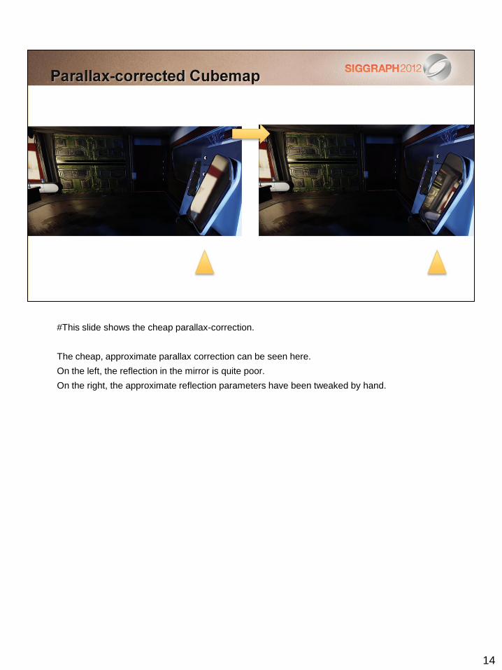
The cheap, approximate parallax correction can be seen here.
On the left, the reflection in the mirror is quite poor.
On the right, the approximate reflection parameters have been tweaked by hand.
15
#This slide describe the mixing cubemaps step.
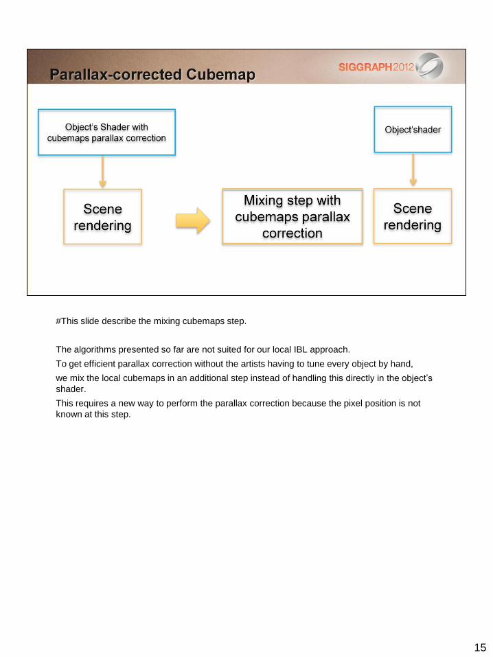
The algorithms presented so far are not suited for our local IBL approach.
To get efficient parallax correction without the artists having to tune every object by hand,
we mix the local cubemaps in an additional step instead of handling this directly in the object’s
shader.
This requires a new way to perform the parallax correction because the pixel position is not
known at this step.
16
17
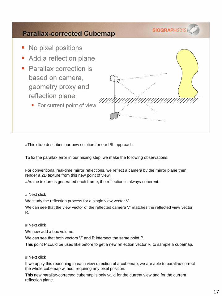
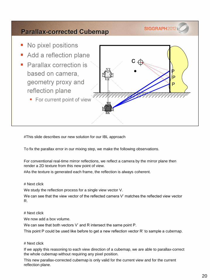
#This slide describes our new solution for our IBL approach
To fix the parallax error in our mixing step, we make the following observations.
For conventional real-time mirror reflections, we reflect a camera by the mirror plane then
render a 2D texture from this new point of view.
#As the texture is generated each frame, the reflection is always coherent.
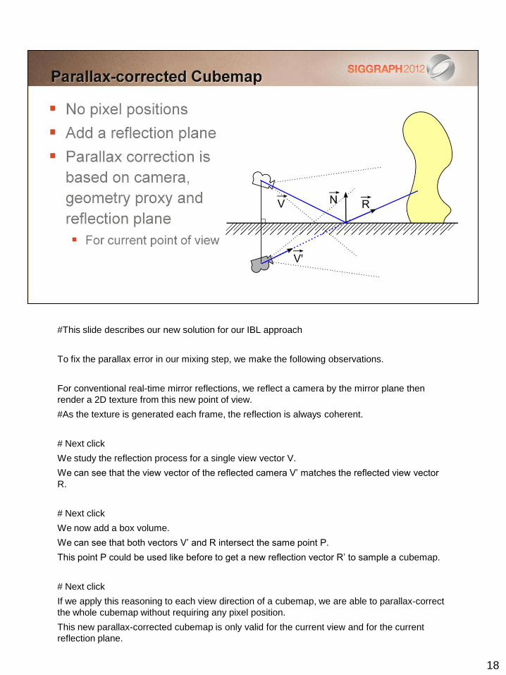
# Next click
We study the reflection process for a single view vector V.
We can see that the view vector of the reflected camera V’ matches the reflected view vector
R.
# Next click
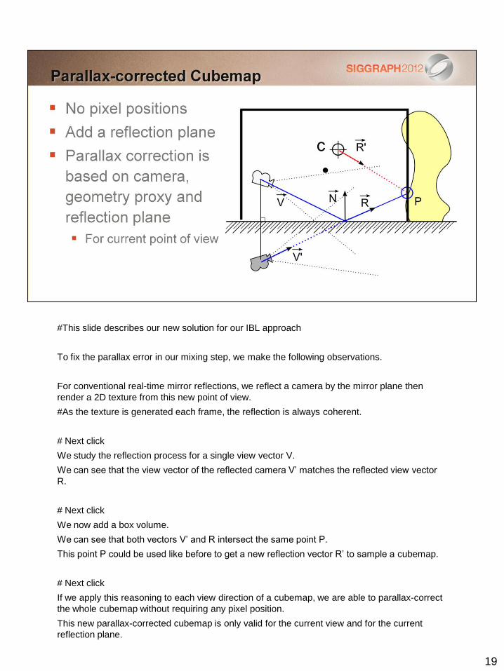
We now add a box volume.
We can see that both vectors V’ and R intersect the same point P.
This point P could be used like before to get a new reflection vector R’ to sample a cubemap.
# Next click
If we apply this reasoning to each view direction of a cubemap, we are able to parallax-correct
the whole cubemap without requiring any pixel position.
This new parallax-corrected cubemap is only valid for the current view and for the current
reflection plane.
18
#This slide describes our new solution for our IBL approach
To fix the parallax error in our mixing step, we make the following observations.
For conventional real-time mirror reflections, we reflect a camera by the mirror plane then
render a 2D texture from this new point of view.
#As the texture is generated each frame, the reflection is always coherent.
# Next click
We study the reflection process for a single view vector V.
We can see that the view vector of the reflected camera V’ matches the reflected view vector
R.
# Next click
We now add a box volume.
We can see that both vectors V’ and R intersect the same point P.
This point P could be used like before to get a new reflection vector R’ to sample a cubemap.
# Next click
If we apply this reasoning to each view direction of a cubemap, we are able to parallax-correct
the whole cubemap without requiring any pixel position.
This new parallax-corrected cubemap is only valid for the current view and for the current
reflection plane.
19
#This slide describes our new solution for our IBL approach
To fix the parallax error in our mixing step, we make the following observations.
For conventional real-time mirror reflections, we reflect a camera by the mirror plane then
render a 2D texture from this new point of view.
#As the texture is generated each frame, the reflection is always coherent.
# Next click
We study the reflection process for a single view vector V.
We can see that the view vector of the reflected camera V’ matches the reflected view vector
R.
# Next click
We now add a box volume.
We can see that both vectors V’ and R intersect the same point P.
This point P could be used like before to get a new reflection vector R’ to sample a cubemap.
# Next click
If we apply this reasoning to each view direction of a cubemap, we are able to parallax-correct
the whole cubemap without requiring any pixel position.
This new parallax-corrected cubemap is only valid for the current view and for the current
reflection plane.
20
#This slide describes our new solution for our IBL approach
To fix the parallax error in our mixing step, we make the following observations.
For conventional real-time mirror reflections, we reflect a camera by the mirror plane then
render a 2D texture from this new point of view.
#As the texture is generated each frame, the reflection is always coherent.
# Next click
We study the reflection process for a single view vector V.
We can see that the view vector of the reflected camera V’ matches the reflected view vector
R.
# Next click
We now add a box volume.
We can see that both vectors V’ and R intersect the same point P.
This point P could be used like before to get a new reflection vector R’ to sample a cubemap.
# Next click
If we apply this reasoning to each view direction of a cubemap, we are able to parallax-correct
the whole cubemap without requiring any pixel position.
This new parallax-corrected cubemap is only valid for the current view and for the current
reflection plane.
21
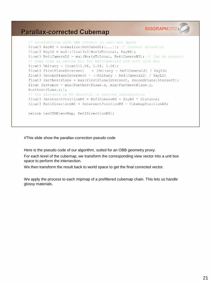
#This slide show the parallax-correction pseudo code
Here is the pseudo code of our algorithm, suited for an OBB geometry proxy.
For each texel of the cubemap, we transform the corresponding view vector into a unit box
space to perform the intersection.
We then transform the result back to world space to get the final corrected vector.
We apply the process to each mipmap of a prefiltered cubemap chain. This lets us handle
glossy materials.
22
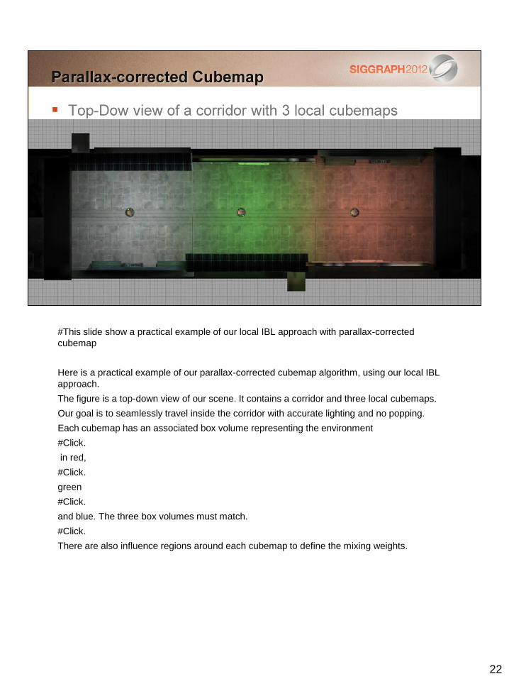
#This slide show a practical example of our local IBL approach with parallax-corrected
cubemap
Here is a practical example of our parallax-corrected cubemap algorithm, using our local IBL
approach.
The figure is a top-down view of our scene. It contains a corridor and three local cubemaps.
Our goal is to seamlessly travel inside the corridor with accurate lighting and no popping.
Each cubemap has an associated box volume representing the environment
#Click.
in red,
#Click.
green
#Click.
and blue. The three box volumes must match.
#Click.
There are also influence regions around each cubemap to define the mixing weights.
23
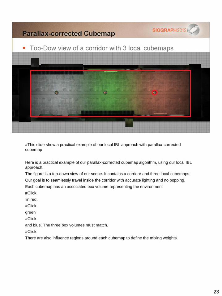
#This slide show a practical example of our local IBL approach with parallax-corrected
cubemap
Here is a practical example of our parallax-corrected cubemap algorithm, using our local IBL
approach.
The figure is a top-down view of our scene. It contains a corridor and three local cubemaps.
Our goal is to seamlessly travel inside the corridor with accurate lighting and no popping.
Each cubemap has an associated box volume representing the environment
#Click.
in red,
#Click.
green
#Click.
and blue. The three box volumes must match.
#Click.
There are also influence regions around each cubemap to define the mixing weights.
24
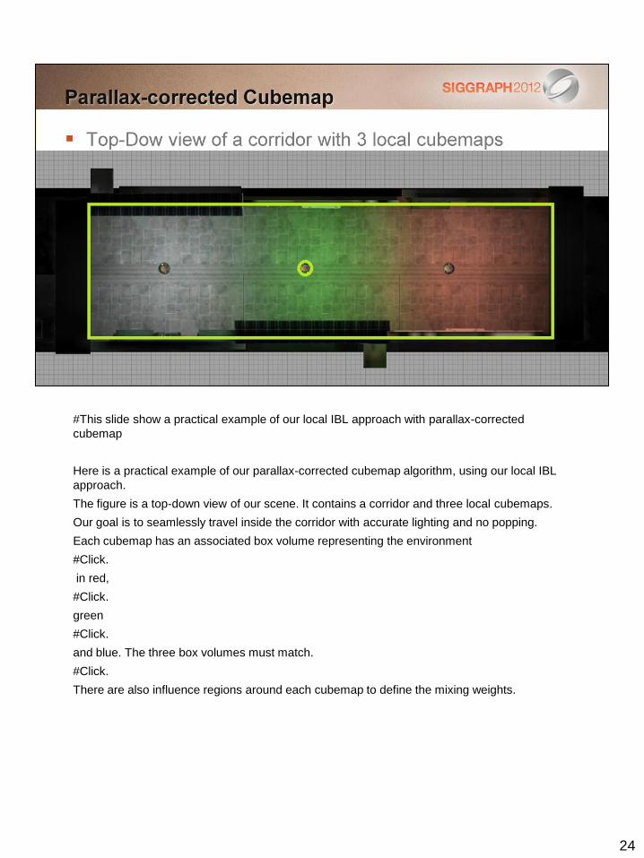
#This slide show a practical example of our local IBL approach with parallax-corrected
cubemap
Here is a practical example of our parallax-corrected cubemap algorithm, using our local IBL
approach.
The figure is a top-down view of our scene. It contains a corridor and three local cubemaps.
Our goal is to seamlessly travel inside the corridor with accurate lighting and no popping.
Each cubemap has an associated box volume representing the environment
#Click.
in red,
#Click.
green
#Click.
and blue. The three box volumes must match.
#Click.
There are also influence regions around each cubemap to define the mixing weights.
25
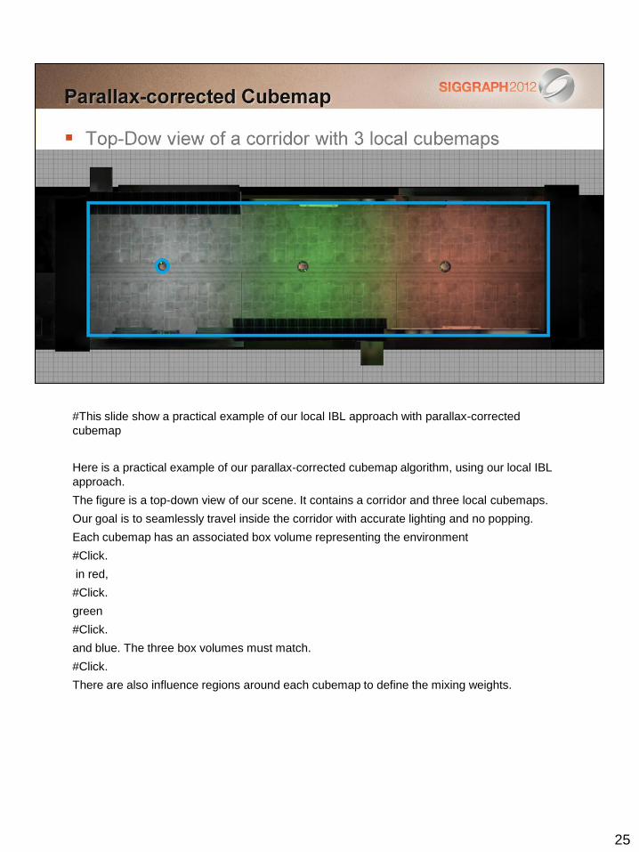
#This slide show a practical example of our local IBL approach with parallax-corrected
cubemap
Here is a practical example of our parallax-corrected cubemap algorithm, using our local IBL
approach.
The figure is a top-down view of our scene. It contains a corridor and three local cubemaps.
Our goal is to seamlessly travel inside the corridor with accurate lighting and no popping.
Each cubemap has an associated box volume representing the environment
#Click.
in red,
#Click.
green
#Click.
and blue. The three box volumes must match.
#Click.
There are also influence regions around each cubemap to define the mixing weights.
26
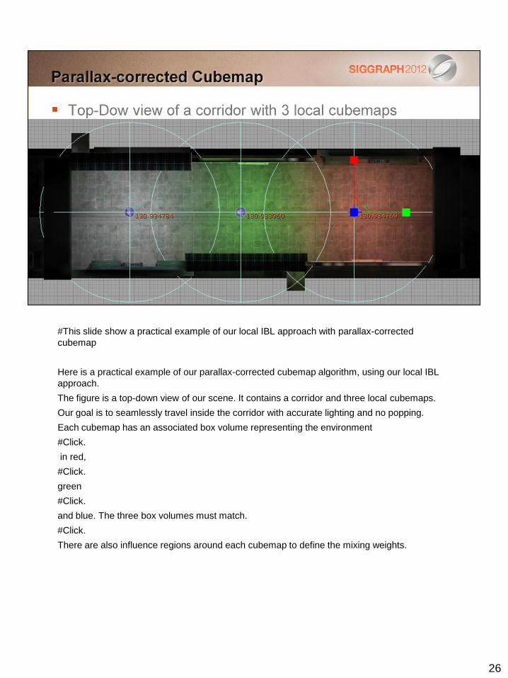
#This slide show a practical example of our local IBL approach with parallax-corrected
cubemap
Here is a practical example of our parallax-corrected cubemap algorithm, using our local IBL
approach.
The figure is a top-down view of our scene. It contains a corridor and three local cubemaps.
Our goal is to seamlessly travel inside the corridor with accurate lighting and no popping.
Each cubemap has an associated box volume representing the environment
#Click.
in red,
#Click.
green
#Click.
and blue. The three box volumes must match.
#Click.
There are also influence regions around each cubemap to define the mixing weights.
27
# Play the video.
#Setup
You can see the cubemaps, their influence regions and their associated box volumes.
# First part.
The ground is set up with a mirror material to better show the result.
This is the parallax error we try to correct.
# Second part.
This is the parallax correction. The transition is smoother thanks to the parallax correction.
Also, the lighting is now consistent, whereas without parallax correction it was not.
It is not possible to get such a result with an infinite cubemap.
#Third part
Moreover, when setting a glossy material it is really difficult to see any problem.
I should advise that a glossy material would require a different setup than mirror material.
28
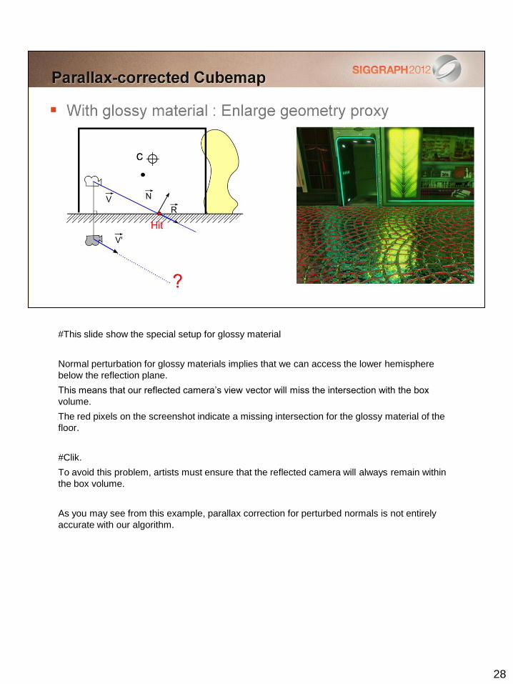
#This slide show the special setup for glossy material
Normal perturbation for glossy materials implies that we can access the lower hemisphere
below the reflection plane.
This means that our reflected camera’s view vector will miss the intersection with the box
volume.
The red pixels on the screenshot indicate a missing intersection for the glossy material of the
floor.
#Clik.
To avoid this problem, artists must ensure that the reflected camera will always remain within
the box volume.
As you may see from this example, parallax correction for perturbed normals is not entirely
accurate with our algorithm.
29
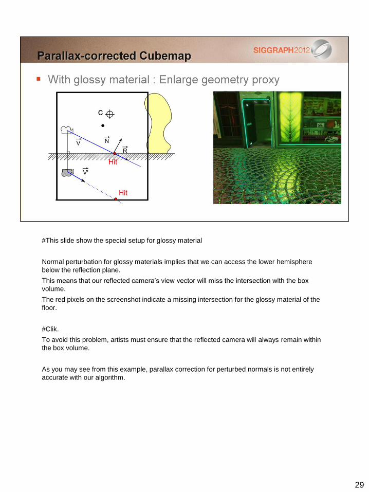
#This slide show the special setup for glossy material
Normal perturbation for glossy materials implies that we can access the lower hemisphere
below the reflection plane.
This means that our reflected camera’s view vector will miss the intersection with the box
volume.
The red pixels on the screenshot indicate a missing intersection for the glossy material of the
floor.
#Clik.
To avoid this problem, artists must ensure that the reflected camera will always remain within
the box volume.
As you may see from this example, parallax correction for perturbed normals is not entirely
accurate with our algorithm.
30
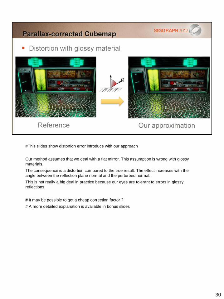
#This slides show distortion error introduce with our approach
Our method assumes that we deal with a flat mirror. This assumption is wrong with glossy
materials.
The consequence is a distortion compared to the true result. The effect increases with the
angle between the reflection plane normal and the perturbed normal.
This is not really a big deal in practice because our eyes are tolerant to errors in glossy
reflections.
# It may be possible to get a cheap correction factor ?
# A more detailed explanation is available in bonus slides
31
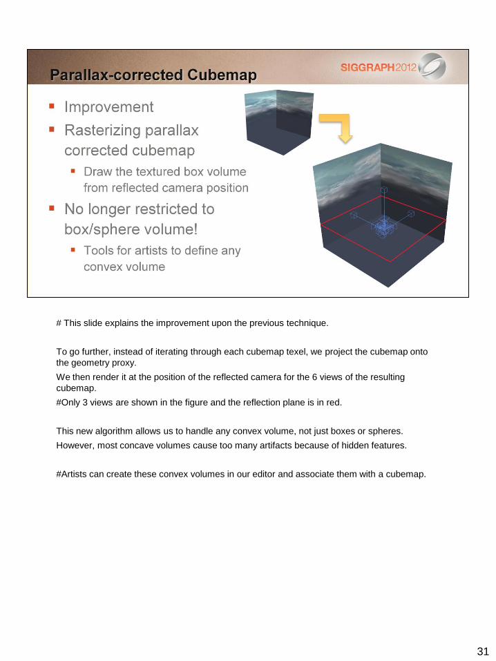
# This slide explains the improvement upon the previous technique.
To go further, instead of iterating through each cubemap texel, we project the cubemap onto
the geometry proxy.
We then render it at the position of the reflected camera for the 6 views of the resulting
cubemap.
#Only 3 views are shown in the figure and the reflection plane is in red.
This new algorithm allows us to handle any convex volume, not just boxes or spheres.
However, most concave volumes cause too many artifacts because of hidden features.
#Artists can create these convex volumes in our editor and associate them with a cubemap.
32
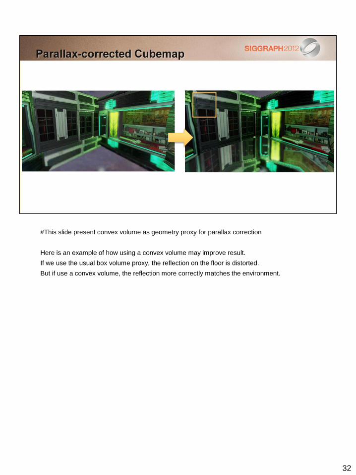
#This slide present convex volume as geometry proxy for parallax correction
Here is an example of how using a convex volume may improve result.
If we use the usual box volume proxy, the reflection on the floor is distorted.
But if use a convex volume, the reflection more correctly matches the environment.
33
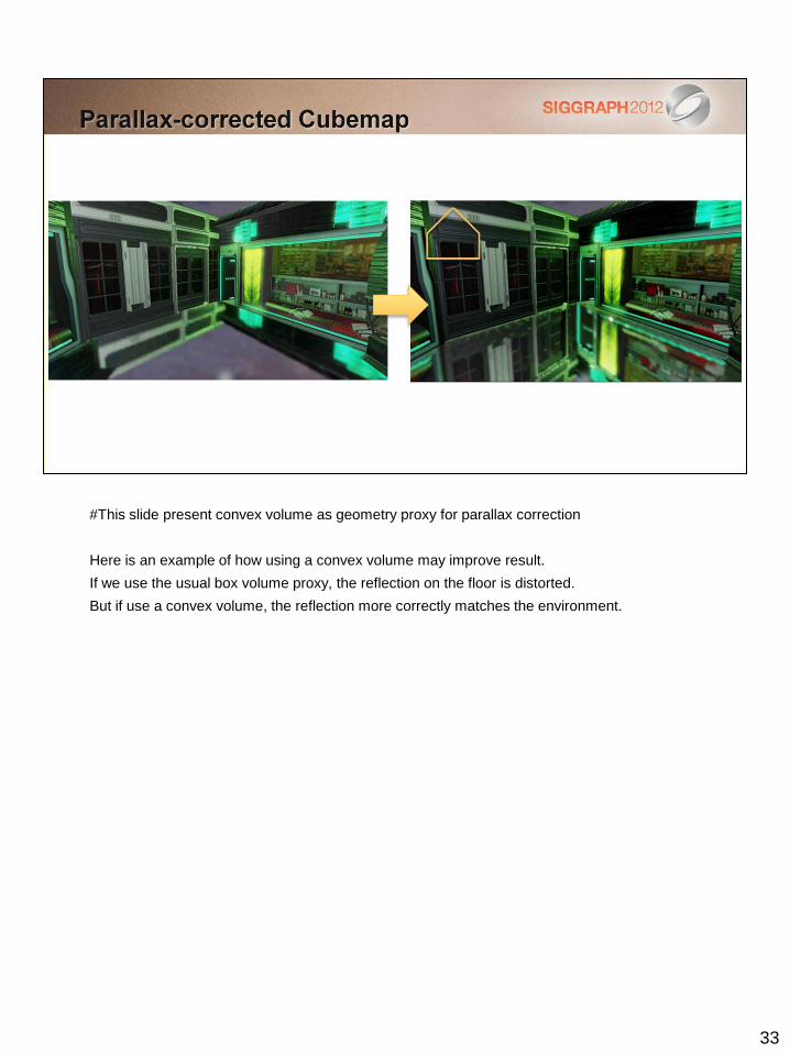
#This slide present convex volume as geometry proxy for parallax correction
Here is an example of how using a convex volume may improve result.
If we use the usual box volume proxy, the reflection on the floor is distorted.
But if use a convex volume, the reflection more correctly matches the environment.
34
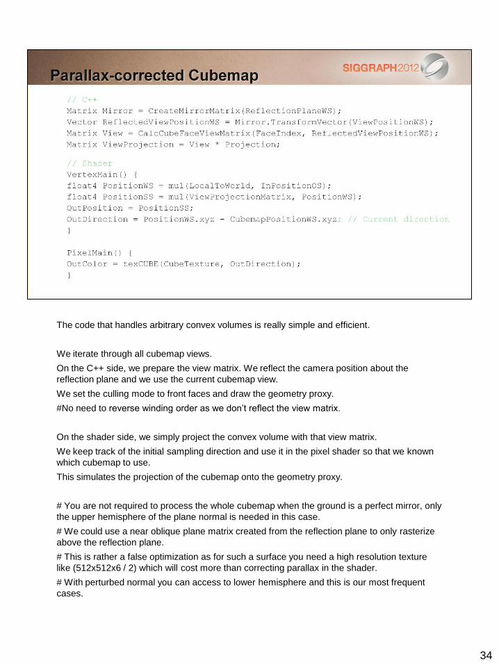
The code that handles arbitrary convex volumes is really simple and efficient.
We iterate through all cubemap views.
On the C++ side, we prepare the view matrix. We reflect the camera position about the
reflection plane and we use the current cubemap view.
We set the culling mode to front faces and draw the geometry proxy.
#No need to reverse winding order as we don’t reflect the view matrix.
On the shader side, we simply project the convex volume with that view matrix.
We keep track of the initial sampling direction and use it in the pixel shader so that we known
which cubemap to use.
This simulates the projection of the cubemap onto the geometry proxy.
# You are not required to process the whole cubemap when the ground is a perfect mirror, only
the upper hemisphere of the plane normal is needed in this case.
# We could use a near oblique plane matrix created from the reflection plane to only rasterize
above the reflection plane.
# This is rather a false optimization as for such a surface you need a high resolution texture
like (512x512x6 / 2) which will cost more than correcting parallax in the shader.
# With perturbed normal you can access to lower hemisphere and this is our most frequent
cases.
35
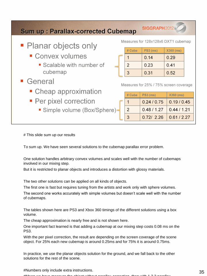
# This slide sum up our results
To sum up. We have seen several solutions to the cubemap parallax error problem.
One solution handles arbitrary convex volumes and scales well with the number of cubemaps
involved in our mixing step.
But it is restricted to planar objects and introduces a distortion with glossy materials.
The two other solutions can be applied on all kinds of objects.
The first one is fast but requires tuning from the artists and work only with sphere volumes.
The second one works accurately with simple volumes but doesn’t scale well with the number
of cubemaps.
The tables shown here are PS3 and Xbox 360 timings of the different solutions using a box
volume.
The cheap approximation is nearly free and is not shown here.
One important fact learned is that adding a cubemap at our mixing step costs 0.08 ms on the
PS3.
With the per pixel correction, the result are depending on the screen coverage of the scene
object. For 25% each new cubemap is around 0.25ms and for 75% it is around 0.75ms.
In practice, we use the planar objects solution for the ground, and we fall back to the other
solutions for the rest of the scene.
#Numbers only include extra instructions.
#Mean we have measure the object without parallax-correction, then with 1,2,3 parallax-
36
37
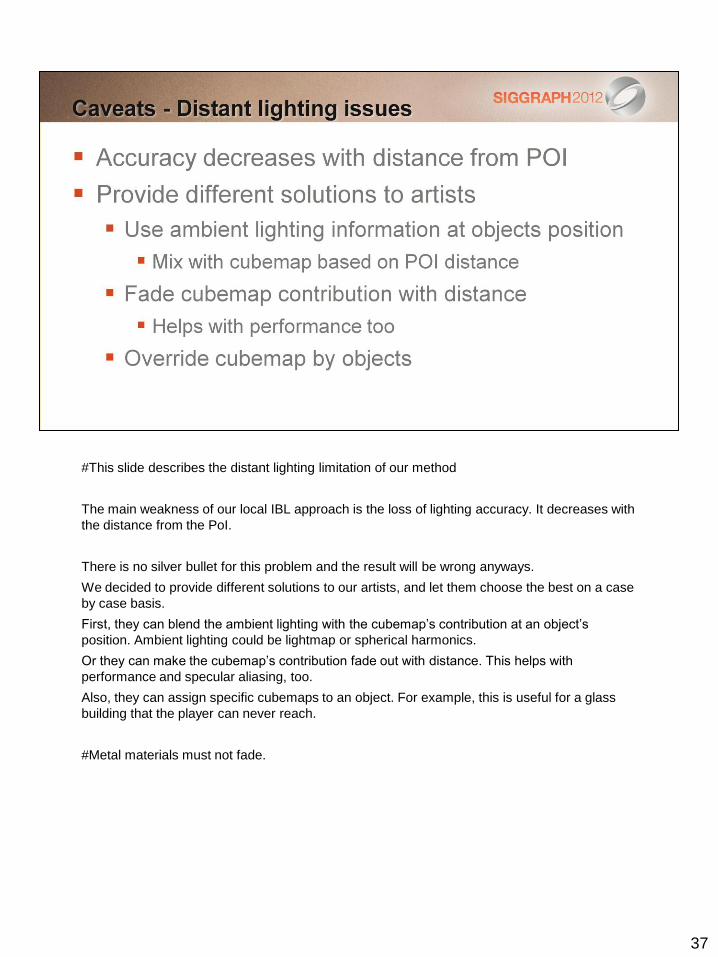
#This slide describes the distant lighting limitation of our method
The main weakness of our local IBL approach is the loss of lighting accuracy. It decreases with
the distance from the PoI.
There is no silver bullet for this problem and the result will be wrong anyways.
We decided to provide different solutions to our artists, and let them choose the best on a case
by case basis.
First, they can blend the ambient lighting with the cubemap’s contribution at an object’s
position. Ambient lighting could be lightmap or spherical harmonics.
Or they can make the cubemap’s contribution fade out with distance. This helps with
performance and specular aliasing, too.
Also, they can assign specific cubemaps to an object. For example, this is useful for a glass
building that the player can never reach.
#Metal materials must not fade.
38
39
#This slide summarizes the takeaways of this talk
To conclude this presentation,
we demonstrated a new local IBL approach, and a set of tools to allow smooth lighting
transitions.
Our approach is cheap and aims to replace costly real-time IBL with a reasonable
approximation.
Our approach require the artists to spend some time to produce better results, and we give
them a lot of freedom to do it.
40
# This slide describes future developments
There is still room for improvement.
We developed additional tools for our method. We describe them in an upcoming article
published in GPU Pro 4, to be released at GDC 2013.

41

42
43

44

45
46
#This slide explains what is the point of interest based on the context
First, our approach requires having a position to gather local cubemaps.
And the question is what position to choose?
In fact, it depends on the context:
We choose the camera in the editor,
We can choose between the Player or the Camera in gameplay phase. Also, we currently use
Player because we find it gives better results for our third person game (camera could turn
around the player and change the lighting otherwise).
For in-game events or cinematics, we leave the choice to the artists.
They can choose any characters or even a dummy location that can be animated by a track.
To avoid lighting popping at end of some cinematic we smoothly move the dummy location to
our player location before re-enabling the control of the player.
47
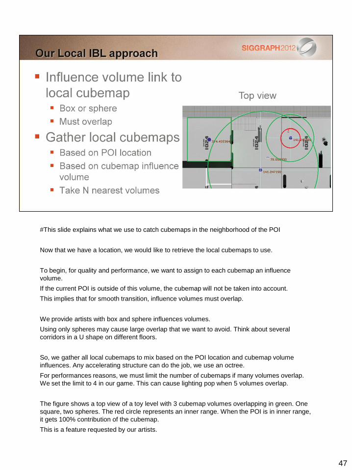
#This slide explains what we use to catch cubemaps in the neighborhood of the POI
Now that we have a location, we would like to retrieve the local cubemaps to use.
To begin, for quality and performance, we want to assign to each cubemap an influence
volume.
If the current POI is outside of this volume, the cubemap will not be taken into account.
This implies that for smooth transition, influence volumes must overlap.
We provide artists with box and sphere influences volumes.
Using only spheres may cause large overlap that we want to avoid. Think about several
corridors in a U shape on different floors.
So, we gather all local cubemaps to mix based on the POI location and cubemap volume
influences. Any accelerating structure can do the job, we use an octree.
For performances reasons, we must limit the number of cubemaps if many volumes overlap.
We set the limit to 4 in our game. This can cause lighting pop when 5 volumes overlap.
The figure shows a top view of a toy level with 3 cubemap volumes overlapping in green. One
square, two spheres. The red circle represents an inner range. When the POI is in inner range,
it gets 100% contribution of the cubemap.
This is a feature requested by our artists.
48
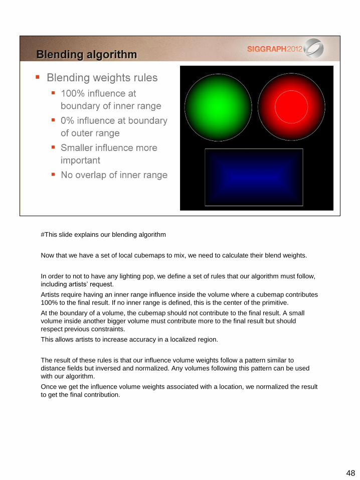
#This slide explains our blending algorithm
Now that we have a set of local cubemaps to mix, we need to calculate their blend weights.
In order to not to have any lighting pop, we define a set of rules that our algorithm must follow,
including artists’ request.
Artists require having an inner range influence inside the volume where a cubemap contributes
100% to the final result. If no inner range is defined, this is the center of the primitive.
At the boundary of a volume, the cubemap should not contribute to the final result. A small
volume inside another bigger volume must contribute more to the final result but should
respect previous constraints.
This allows artists to increase accuracy in a localized region.
The result of these rules is that our influence volume weights follow a pattern similar to
distance fields but inversed and normalized. Any volumes following this pattern can be used
with our algorithm.
Once we get the influence volume weights associated with a location, we normalized the result
to get the final contribution.
49
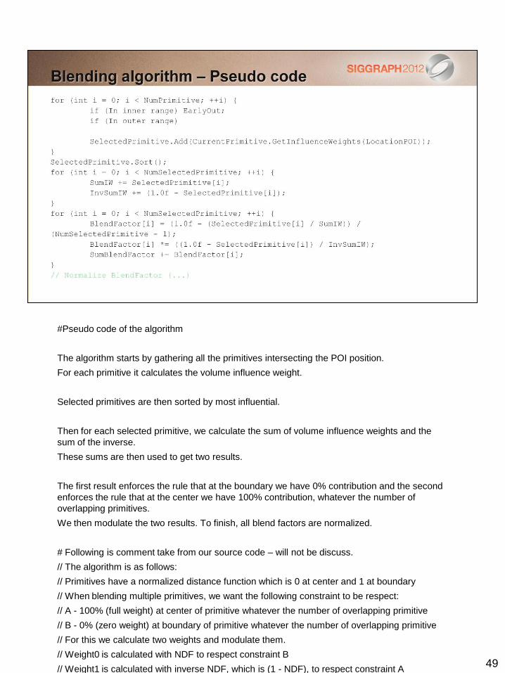
#Pseudo code of the algorithm
The algorithm starts by gathering all the primitives intersecting the POI position.
For each primitive it calculates the volume influence weight.
Selected primitives are then sorted by most influential.
Then for each selected primitive, we calculate the sum of volume influence weights and the
sum of the inverse.
These sums are then used to get two results.
The first result enforces the rule that at the boundary we have 0% contribution and the second
enforces the rule that at the center we have 100% contribution, whatever the number of
overlapping primitives.
We then modulate the two results. To finish, all blend factors are normalized.
# Following is comment take from our source code – will not be discuss.
// The algorithm is as follows:
// Primitives have a normalized distance function which is 0 at center and 1 at boundary
// When blending multiple primitives, we want the following constraint to be respect:
// A - 100% (full weight) at center of primitive whatever the number of overlapping primitive
// B - 0% (zero weight) at boundary of primitive whatever the number of overlapping primitive
// For this we calculate two weights and modulate them.
// Weight0 is calculated with NDF to respect constraint B
// Weight1 is calculated with inverse NDF, which is (1 - NDF), to respect constraint A
50
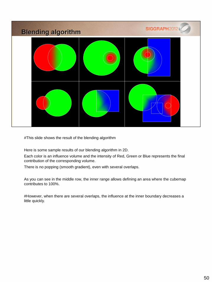
#This slide shows the result of the blending algorithm
Here is some sample results of our blending algorithm in 2D.
Each color is an influence volume and the intensity of Red, Green or Blue represents the final
contribution of the corresponding volume.
There is no popping (smooth gradient), even with several overlaps.
As you can see in the middle row, the inner range allows defining an area where the cubemap
contributes to 100%.
#However, when there are several overlaps, the influence at the inner boundary decreases a
little quickly.
51
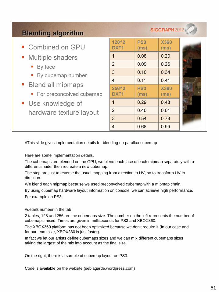
#This slide gives implementation details for blending no-parallax cubemap
Here are some implementation details,
The cubemaps are blended on the GPU, we blend each face of each mipmap separately with a
different shader then recreate a new cubemap.
The step are just to reverse the usual mapping from direction to UV, so to transform UV to
direction.
We blend each mipmap because we used preconvolved cubemap with a mipmap chain.
By using cubemap hardware layout information on console, we can achieve high performance.
For example on PS3,
#details number in the tab
2 tables, 128 and 256 are the cubemaps size. The number on the left represents the number of
cubemaps mixed. Times are given in milliseconds for PS3 and XBOX360.
The XBOX360 platform has not been optimized because we don’t require it (In our case and
for our team size, XBOX360 is just faster).
In fact we let our artists define cubemaps sizes and we can mix different cubemaps sizes
taking the largest of the mix into account as the final size.
On the right, there is a sample of cubemap layout on PS3.
Code is available on the website (seblagarde.wordpress.com)
52
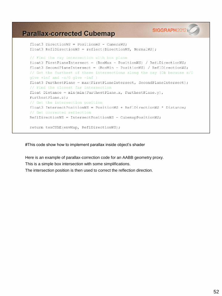
#This code show how to implement parallax inside object’s shader
Here is an example of parallax-correction code for an AABB geometry proxy.
This is a simple box intersection with some simplifications.
The intersection position is then used to correct the reflection direction.
53
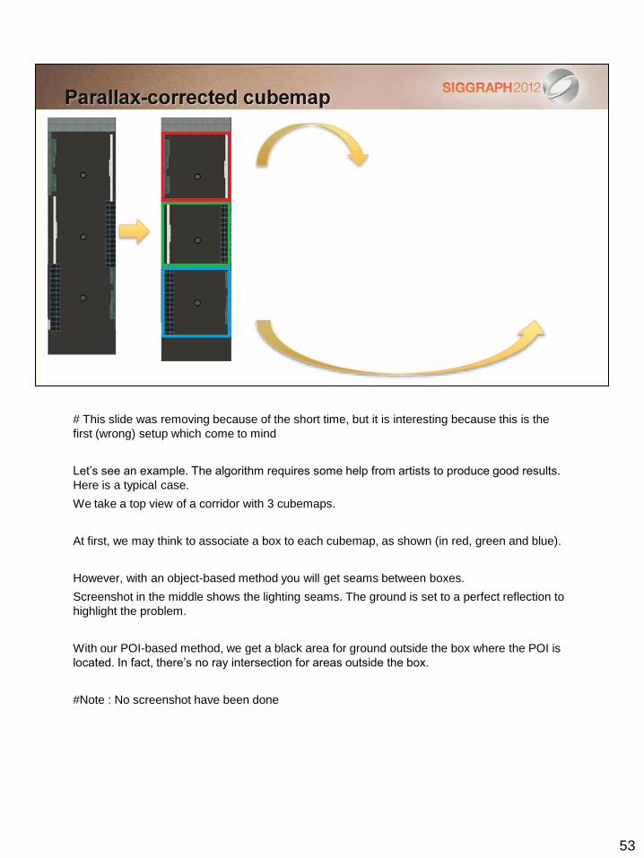
# This slide was removing because of the short time, but it is interesting because this is the
first (wrong) setup which come to mind
Let’s see an example. The algorithm requires some help from artists to produce good results.
Here is a typical case.
We take a top view of a corridor with 3 cubemaps.
At first, we may think to associate a box to each cubemap, as shown (in red, green and blue).
However, with an object-based method you will get seams between boxes.
Screenshot in the middle shows the lighting seams. The ground is set to a perfect reflection to
highlight the problem.
With our POI-based method, we get a black area for ground outside the box where the POI is
located. In fact, there’s no ray intersection for areas outside the box.
#Note : No screenshot have been done
54
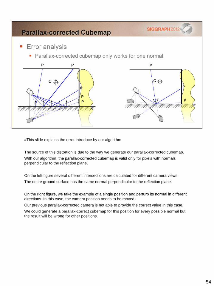
#This slide explains the error introduce by our algorithm
The source of this distortion is due to the way we generate our parallax-corrected cubemap.
With our algorithm, the parallax-corrected cubemap is valid only for pixels with normals
perpendicular to the reflection plane.
On the left figure several different intersections are calculated for different camera views.
The entire ground surface has the same normal perpendicular to the reflection plane.
On the right figure, we take the example of a single position and perturb its normal in different
directions. In this case, the camera position needs to be moved.
Our previous parallax-corrected camera is not able to provide the correct value in this case.
We could generate a parallax-correct cubemap for this position for every possible normal but
the result will be wrong for other positions.
55


![Sébastien Plutniak – Curriculum vitæ · [6] 2020 Plutniak,Sébastien[2020b],«Durecoursauxsciencesstudiesdanslescontroverses scientifiques:uneillustrationarchéologique»,Zilsel.Science,technique,société,7,](https://static.fdocuments.in/doc/165x107/5fb061c5788a8d41a256a2b7/sbastien-plutniak-a-curriculum-vit-6-2020-plutniaksbastien2020bdurecoursauxsciencesstudiesdanslescontroverses.jpg)

