RESEARCH Open Access

Lessons from April 6, 2009 L’Aquilaearthquake to enhance microzoningstudies in near-field urban areasGiovanna Vessia1*, Mario Luigi Rainone1, Angelo De Santis2 and Giuliano D’Elia1

Abstract

This study focuses on two weak points of the present procedure to carry out microzoning study in near-field areas: (1) theGround Motion Prediction Equations (GMPEs), commonly used in the reference seismic hazard (RSH) assessment; (2) theambient noise measurements to define the natural frequency of the near surface soils and the bedrock depth. Thelimitations of these approaches will be discussed throughout the paper based on the worldwide and Italian experiencesperformed after the 2009 L’Aquila earthquake and then confirmed by the most recent 2012 Emilia Romagna earthquakeand the 2016–17 Central Italy seismic sequence. The critical issues faced are (A) the high variability of peak groundacceleration (PGA) values within the first 20–30 km far from the source which are not robustly interpolated by the GMPEs,(B) at the level 1 microzoning activity, the soil seismic response under strong motion shaking is characterized bymicrotremors’ horizontal to vertical spectral ratios (HVSR) according to Nakamura’s method. This latter technique iscommonly applied not being fully compliant with the rules fixed by European scientists in 2004, after a 3-year projectnamed Site EffectS assessment using AMbient Excitations (SESAME). Hereinafter, some “best practices” from recent Italianand International experiences of seismic hazard estimation and microzonation studies are reported in order to putforward two proposals: (a) to formulate site-specific GMPEs in near-field areas in terms of PGA and (b) to recordmicrotremor measurements following accurately the SESAME advice in order to get robust and repeatable HVSR valuesand to limit their use to those geological contests that are actually horizontally layered.

Keywords: Reference seismic hazard map, Seismic microzoning study, HVSR Nakamura’s method, GMPEs

IntroductionOn April 6, 2009, at 1:32 a.m. (local time) an Mw 6.3earthquake with shallow hypocentral depth (8.3 km) hitthe city of L’Aquila and several municipalities within theAterno Valley. This earthquake can be considered one ofthe most mournful seismic event in Italy since 1980 al-though its magnitude was moderately-high: 308 fatalitiesand 60.000 people displaced (data source http://www.protezionecivile.it) and estimated damages for 1894M€(data source http://www.ngdc.noaa.gov). These numbersshowed how dangerous can be an unexpected seismic

event in urbanized territories where no preventive ac-tions have been addressed to reduce seismic risk. Hence,meanwhile, some actions were implementing in thepost-earthquake time such as updating the referenceItalian hazard map (by the Decree OPCM n. 3519 on 28April 2006) and drawing microzoning maps to be usedin the reconstruction stage, two major earthquakesstruck the Emilia Romagna Region (in the Northern partof Italy), causing 27 deaths and widespread damage. Thefirst, with Mw 6.1, occurred on 20 May at 04:03 localtime (02:03 UTC) and was located at about 36 km northof the city of Bologna. Then, a second major earthquake(Mw 5.9) occurred on 29 May 2012, in the same area,causing widespread damage, particularly to buildingsalready weakened by the 20 May earthquake. Later on,

© The Author(s). 2020 Open Access This article is licensed under a Creative Commons Attribution 4.0 International License,which permits use, sharing, adaptation, distribution and reproduction in any medium or format, as long as you giveappropriate credit to the original author(s) and the source, provide a link to the Creative Commons licence, and indicate ifchanges were made. The images or other third party material in this article are included in the article's Creative Commonslicence, unless indicated otherwise in a credit line to the material. If material is not included in the article's Creative Commonslicence and your intended use is not permitted by statutory regulation or exceeds the permitted use, you will need to obtainpermission directly from the copyright holder. To view a copy of this licence, visit http://creativecommons.org/licenses/by/4.0/.

* Correspondence: g.vessia@unich.it1Department of Engineering and Geology, University “G.d’Annunzio” ofChieti-Pescara, Via dei Vestini 31, 66013 Chieti, Scalo (CH), ItalyFull list of author information is available at the end of the article

Geoenvironmental DisastersVessia et al. Geoenvironmental Disasters (2020) 7:11 https://doi.org/10.1186/s40677-020-00147-x

the 2016–17 Central Italy Earthquake Sequence oc-curred, consisting of several moderately-high magnitudeearthquakes between Mw 5.5 and Mw 6.5, from Aug 24,2016, to Jan 18, 2017, each centered in a different butclose location and with its own sequences of aftershocks,spanning several months. The seismic sequence killedabout 300 people and injured the other 396. Worldwide,several other strong earthquakes (eg. 1998 Northridgeearthquake, 2004 Parkfield earthquake, 2010 Canterburyand 2011 and 2017 Christchurch earthquakes, 2018Sulawesi earthquake) produced devastating effects in thesame time span. All these events show the need to carryout efficient microzoning studies to plan vulnerabilityreductions of urban structures and promoting the resili-ence of the human communities in seismic territories.After the 2009 L’Aquila earthquake, the microzoningstudies have been introduced in Italy by law and theGuidelines for Seismic Microzonation (ICMS 2008) havebeen issued to accomplish these studies according to themost updated international scientific findings. Theseguidelines provide the local administrators with an effi-cient tool for seismic microzoning study to predictingthe subsoil behavior under seismic shaking. Unfortu-nately, the ICMS does not give special recommendationsfor urbanized near field areas (NFAs). The microzoningactivity concerning urbanized territories as suggest byICMS (2008) is made up of four steps:

1- Estimating the reference seismic hazard to providethe input peak horizontal ground acceleration(PGA) at each point on the national territory andthe normalized response spectrum at each site.

2- Dynamic characterization of soil deposits overlayingthe seismic bedrock at each urban center in orderto draw the microzoning maps (MM) at three mainknowledge levels.

3- The Level 1 MM consists of geo-lithological mapsof the surficial deposits that show typical succes-sions and the amplified frequency map drawnthrough the measurements of microtremors elabo-rated by horizontal to vertical spectral ratio HVSRNakamura’s technique. Nakamura’s method (1989),the horizontal to vertical noise components are cal-culated to derive the natural frequency of surficialsoft deposits and their thickness.

4- The Level 2/3 MM consists of drawing maps afterperforming the numerical analyses of (a) seismiclocal amplification factors in terms of accelerationFA and velocity FV; (b) liquefaction potential LPand (c) permanent displacements due to seismicallyinduced slope instability.

After 10 years of training the ICMS and the relatedmethods, it is now the time to start analyzing some arisen

weak points. Starting from the large data acquired world-wide on recent strong motion earthquakes, the experiencesdeveloped in seismic hazard assessment, and the site-specific seismic response characterization carried out by thewriting authors after the 2009 L’Aquila earthquake, theaforementioned weak points (related to some aspects of thesteps 1 and 3) are hereinafter discussed and some proposalsare made to improve the efficiency of the microzoningstudies especially in NFAs.In this paper, after a brief background section on the

procedures to accomplish the reference seismic hazard as-sessment (background section), the methods to calculatethe Ground Motion Prediction Equations (GMPEs) andthe HVSR (Nakamura’s method) are briefly recalled insection 2. Then in section 3, the results from observationsof recorded peak ground acceleration (PGA) and pseudo-spectral acceleration (PSA) values within the NFAs fromthe L’Aquila earthquake and other worldwide strongearthquakes have been discussed. In addition, some appli-cations of Nakamura’s procedure to characterize the nat-ural frequency of the sites throughout the Aterno Valleyhave been discussed. Finally, in the conclusion section,some relevant points drawn from the discussed microzon-ing experiences have been highlighted to improve the effi-ciency of the microzonation studies in urban centersespecially located in NFAs.

Background on seismic hazard assessmentSeveral theoretical and experimental studies performedworldwide in the last 50 years (see Kramer 1996 and thereference herein), highlighted that seismic shaking inten-sity is due to the magnitude of the earthquake generatedat the source, to the travel paths of the seismic waves fromthe source to the buried or outcropping bedrock (that iscalled reference seismic hazard RSH) and the additionalphenomena of local amplification or de-amplification takeplace where soil deposits overlay the rocky bedrock,named local seismic response LSR (Paolucci 2002; Vessiaand Venisti 2011; Vessia et al. 2011; Vessia and Russo2013; Vessia et al. 2013, 2017; Boncio et al. 2018, amongothers). The RSH maps drawn worldwide on national terri-tories do not take into account the results of LSR studies.The pioneering work by Signanini et al. (1983) after the

1979 Friuli earthquake confirmed the observations on theground: local seismic effects could enlarge the referencedhazard at a site by 2–3 times in terms of MCS scale Inten-sity but also in PGA values owing to the local morpho-logical and stratigraphic settings. Such RSL is particularlyevident in near field areas, from then on named NFAs. TheNFAs have been defined among others by Boore (2014a) asthe Fault Damage Zones. These areas cannot be uniquelyidentified depending on the source rupture mechanisms,the surficial soil deposits and the multiple calculationmethods used for measuring the distance between the

Vessia et al. Geoenvironmental Disasters (2020) 7:11 Page 2 of 15

seismic stations and the source. Especially in these areas,about the first 30 km aside the source, spot-like amplifica-tions are the common amplification pattern capturedthrough the Maximum Intensity Felt maps. These maps es-timate the differentiated damages suffered by buildings andurban structures by means of the Macroseismic Intensityscale (e.g. Mercalli-Cancani-Sieberg MCS scale, EuropeanMacroseismic scale EMS, Modified Mercalli Intensity MMIscale). One of the Maximum Intensity Felt maps on theItalian territory was drawn by Boschi et al. (1995). Theytook into account the seismic events that occurred from 1

to 1992 AD with a minimum intensity felt of VI MCS.This latter value is the one commonly used to highlightthose areas where seismic events caused relevant damagesto dwellings and infrastructures, ranging from severe dam-ages to collapse. Boschi et al. (1995) map is reported inFig. 1: it showed IX-X MCS at L’Aquila district based onhistorical earthquakes that are in agreement with the seis-mic intensity map drawn by Galli and Camassi (2009)after the mainshock of 2009 L’Aquila earthquake. Thismap is also in very good agreement with other recentearthquakes such as the 2012 Emilia Romagna and 2016–

Fig. 1 Italian Maximum Intensity felt map (After Boschi et al. 1995, modified) with the areas of two recent Italian earthquake sequencesconsidered in the present work

Vessia et al. Geoenvironmental Disasters (2020) 7:11 Page 3 of 15

17 Central Italy earthquakes (Fig. 1). Moreover, Boschiet al. (1995), Midorikawa (2002) and more recently, Pao-lini et al. (2012) proposed a direct use of the MaximumFelt Intensity maps to highlight those areas where the ref-erence seismic hazard is largely increased by the localamplificated responses of soil deposits, that is the NFAs.The most used method to perform the reference seis-

mic hazard assessment has been conceived in the late‘60s. It is Cornell’s method (1968) that was implementedinto a numerical code by Mc Guire (1978). Cornell(1968) introduced the Probabilistic Seismic Hazard As-sessment (PSHA) method to carry out the reference seis-mic hazard at a site considering the contribution of theseismic source and the travel path of the seismic wavesby considering the uncertainties related to these estima-tions. This method consists of four steps (Kramer 1996),as illustrated in Fig. 2:

STEP 1. To identify the seismogenic sources as singlefaults and faulting regions in terms of magnitudeamplitude generated at different time spans. Theprobabilistic approach to such a characterization needs toknow the rate of the earthquake at different magnitudes atthe site and the spatial distribution of the fault segment orthe source volume that can be activated.STEP 2_1. To calculate the seismic rate in a region theGutenberg-Richter law is used, where a and b coeffi-cients are drawn by interpolating numerous data froma database of seismic events (instrumental and non-instrumental) available for a limited number of source

areas and affected by the lack of completeness distor-tions. The earthquake occurrence probability is esti-mated by means of a Poisson distribution over timethat is independent of the time span of the last strongseismic event.STEP 2_2. To calculate the spatial distribution of theseismic events alongside a fault zone is a characterdifficult to get known and the spatial distribution ofearthquake sources within a seismogenic area iscommonly assumed uniformly distributed.STEP 3. To define the ground motion predictionequations GMPEs that enable to predict, at differentmagnitude ranges, the decrease with the distance fromthe seismic source of the strong motion parameterassumed to be representative of the earthquake at a site.STEP 4. To calculate the probability of exceedance of atarget shaking value of the considered ground motionparameter, i.e. PGA, in a time span at a chosen site, dueto the contribution of different seismogenic sources.

The previous 4 steps attempt to take into account severalsources of uncertainties, such as the limited knowledgeabout the fault activity, the qualitative and documental esti-mations of the past earthquake effects at the sites, the lackof completeness of the seismic catalogs (meaning that thedatabase of the seismic events is populated by several datarelated to both low and high magnitude ones) and the de-pendency among the recorded strong seismic events. Inaddition, the distortions in Gutenberg-Richter law, definedfor different regions worldwide and the uncertainties related

Fig. 2 Cornell’s probabilistic seismic hazard assessment (PSHA) explained in four steps. The blue house represents the site under study

Vessia et al. Geoenvironmental Disasters (2020) 7:11 Page 4 of 15

to the GMPEs can generate underestimations of the seismicshaking parameters (i.e. PGA) at specific sites where localseismic effects are relevant (Paolucci 2002; Vessia andVenisti 2011; Vessia and Russo 2013; Vessia et al. 2013;Yagoub 2015; Miyajima et al. 2019; Lanzo et al. 2019; amongothers). Logic trees are commonly used to take into accountdifferent formulations of GMPEs and several Gutenberg-Richter rates of magnitude occurrence (Kramer 1996).Molina et al. (2001) pointed out that the PSHA has its

strength in the systematic parameterization of seismicityand the way in which also epistemic uncertainties are car-ried out through the computations into the final results.Recently, alternative approaches to PSHA calculation

have been suggested, such as through extensions of thezonation method (Frankel 1995; Frankel et al. 1996, 2000;Perkins 2000) where multiple source zones, parametersmoothing and quantification of geology and active faultshave been successfully applied. The Frankel et al. (1996)method applied a Gaussian function to smooth a-values(within Gutenberg-Richter law) from each zone, therebybeing a forerunner for the later zonation-free approachesof Woo (1996). This latter approach tries to amalgamatestatistical consistency with the empirical knowledge of theearthquake catalogue (with its fractal character) into thecomputation of seismic hazard. Furthermore, Jackson andKagan (1999) developed a non-parametric method with acontinuous rate-density function (computed from earth-quake catalogues) used in earthquake forecasting. None-theless, all these methods need a function to propagatethe strong motion parameter values from the source tothe site under study. To this end, the GMPEs are built byinterpolating large databases of seismic records (related tospecific geographical and tectonic environments world-wide), taking into account the contributions of the earth-quake magnitude M and the distance to the seismicsource R, according to the following form (Kramer 1996):

ln Yð Þ ¼ f M;R; Sið Þ ð1Þ

where Y is the ground motion parameter, commonly thepeak ground horizontal acceleration PGA or the spectralacceleration SA at fixed period; Si is related to the sourceand site: they are the refinement terms due to the enlarge-ment of the seismic databases and the possibility of draw-ing specific regional GMPEs.

MethodsThe uncertainty of GMPEs in near field areasSeveral examples of GMPEs are provided in literature(Kramer 1996 among others) while a recent throughoutreview of several possible formulations of GMPEs usedin the USA can be found at the Pacific Earthquake Engin-eering Research center PEER website http://peer.berkeley.edu/publications/peer_reports_complete.html. In Italy, the

GMPEs are built based on the PGAs drawn from theItalian shape wave database of strong motion events(Faccioli 2012; Bindi et al. 2011, 2014; Cauzzi et al. 2014).Commonly, the PGA values represent the strong motionparameter used in microzoning studies but the relatedGMPEs are highly uncertain especially in the first tens ofkilometers as shown in Fig. 3a (Faccioli 2012) and Fig. 4a(Boore 2013). According to Boore (2013, 2014a), faultzone records show significant variability in amplitudeand polarization of PGA, SA especially at low periods(as shown in Fig. 4a) and magnitude saturation beyondMw 6, although the causes of this variability are not easyto be unraveled. The main drawback of the GMPEs is theweakness of their predictivity at a short distance from theseismic source due to two main issues affecting the NFAsworldwide:

1) a few seismic stations installed;2) highly scattered measures of strong motion

parameters, especially in terms of accelerations (i.e.PGA, SA, etc) (Fig. 2, step 3), that do not show anydecreasing trend with distance.

The PGA spatial uncertainties have been observedafter several recent strong earthquakes, such as 2009L’Aquila earthquake (Lanzo et al. 2010; Bergamaschiet al. 2011; Di Giulio et al. 2011), 2011 Christchurch and2010 Darfield earthquakes in New Zealand (Bradley andCubrinovski 2011) (Fig. 5), 2012 Emilia Romagna earth-quake in Italy, 1994 Northridge earthquake in USA(Boore 2004) and 2013 Fivizzano earthquake (Fig. 5). Inthe case of the 2009 L’Aquila earthquake (Fig. 4b), theareal distribution of PGAs around the source seems tobe highly random although they show that the most dra-matic increase occurs where thick soft sediments aremet over rigid bedrocks or where bedrock basin shapescan be recognized. This latter traps the seismic wavesand caused longer duration accelerograms with in-creased amplitudes at short and moderate periods (lowerthan 2 s) (Rainone et al. 2013).The GMPEs based on PGAs tend to saturate for large

earthquakes as the distance from the fault rupture to theobservation point decreases. Boore (2014b) showed thatthe PGA parameter is a poor measure of the ground-motion intensity due to its non-unique correspondenceto the frequency and acceleration content of the shakingwaves (Fig. 4), especially at high frequencies. Further-more, Bradley and Cubrinovski (2011) and Boore (2004)stated that the influence on the amplitude and shape re-sponse by local surface geology and geometrical condi-tions is noted to be much more relevant than theforward directivity and the source-site path on spectralaccelerations in near field areas and for periods shorterthan 3 s.

Vessia et al. Geoenvironmental Disasters (2020) 7:11 Page 5 of 15

Thus, the GMPEs of PGAs within the NFAs are highlyuncertain and cumbersome to be predicted even whenfitted on single seismic events as shown in Fig. 5(Bradley and Cubrinovski 2011; Faccioli 2012; Boore2014b). Faccioli (2012) evidenced 100% of the coefficient

of variation about the mean trend of PGA GMPE versussource-to-site distance (Fig. 3a). This GMPE was builtbased on the ITACA 2010 database (Luzi et al. 2008,http://itaca.mi.ingv.it/ItacaNet_30/#/home) that collectsItalian strong motion shape waves. It is worth noticing

Fig. 4 a Measures of PSA during the Parkfield earthquake 2004 (6 Mw) are reported near the active fault at the measure seismic stations (AfterBoore 2014b, modified); b Onna sector of Aterno River Valley: the records are for an aftershock of 3.2 Ml

Fig. 3 a Ground Motion Prediction Equation (GMPE) of PGA versus the minimum source-to-site distance (After Faccioli 2012, modified): a band ofuncertainty (grey) of GMPEs proposed by Faccioli et al. (2010). b 2008 Boore and Atkinson ground motion prediction equation (BA08 GMPE) ofPGA based on data collected in United States for Magnitude 7.3 Mw, strike-slip fault type and VS30equal to 255 m/s: solid line is the meanequation; dashed lines represent the confidence interval at one standard deviation (After Boore 2013, modified)

Vessia et al. Geoenvironmental Disasters (2020) 7:11 Page 6 of 15

that within the first tens of kilometers from the source,these data indicate that the GMPEs are not accurate inpredicting the PGA values. To avoid the pitfalls inGMPEs based on peak parameters, integral ground mo-tion parameters have been proposed in the literature(Kempton and Stewart 2006; Abrahamson and Silva2008; Campbell and Bozorgnia 2012), such as Arias in-tensity (AI) and cumulative absolute velocity (CAV). Inaddition, Hollenback et al. (2015) and Stewart et al.(2015) formulated new generation GMPEs based on me-dian ground-motion models as part of the Next Gener-ation Attenuation for Central and Eastern NorthAmerica project. They provided a set of adjustments tomedian GMPEs that are necessary to incorporate thesource depth effects and the rupture distances in therange from 0 to 1500 Km. Moreover, the preceding au-thors suggest a distinct expression for the GMPE atshort-distance to the source (by 10 km), that is:

lnGMPE ¼ c1 þ c2 ln RRUP þ hð Þ1=2 ð2Þ

where RRUP is the rupture distance, that is the closestdistance to the earthquake rupture plane (km); c1 and c2are the regression coefficients and h is a “fictitiousdepth” used for ground-motion saturation at closedistances.

Ambient noise measures elaborated by means of theNakamura horizontal to vertical ratio HVSRIn 1989 Nakamura proposed to use the ambient noisemeasurements to derive a seismic property of a site, thatis the frequency range of amplification, through thespectral ratio of horizontal H and vertical V ambient vi-bration (microtremors) components of the recorded sig-nals. If the site does not amplify, the ratio H/V is equal

to 1. The Nakamura method shows the advantage tosolve the troublesome issue to find out a reference site.In fact, it considers the vertical component as the onethat is not modified by the site where horizontal subsoillayers are set and SH seismic waves represent the ambi-ent noise signal content in a quite site (far from urbanor industrial areas). This latter is the reference signalwhereas the horizontal component is the only one thatcan be affected by the amplifying properties of the soils.As a matter of fact, Nakamura assumed that:

– locally random distributed sources of microtremorsgenerate not directional signals almost made up ofshear horizontal or Rayleigh waves;

– the microtremors are confined in the surficial layersbecause the subsoil is made up of soft layeredsediments overlaying a rigid seismic bedrock.

A relevant implication of the Nakamura method is thatthe peaks of the ratio H/V are related to the presence ofhigh acoustic impedance contrast at the depth h thatcan be derived by the following expression:

h ¼ VS

4∙ f 0ð3Þ

where VS is the mean value of the measured shear wavevelocity profile and fo is the amplified frequency mea-sured by means of the noise measurement.The fundamental rules to perform a correct ambient

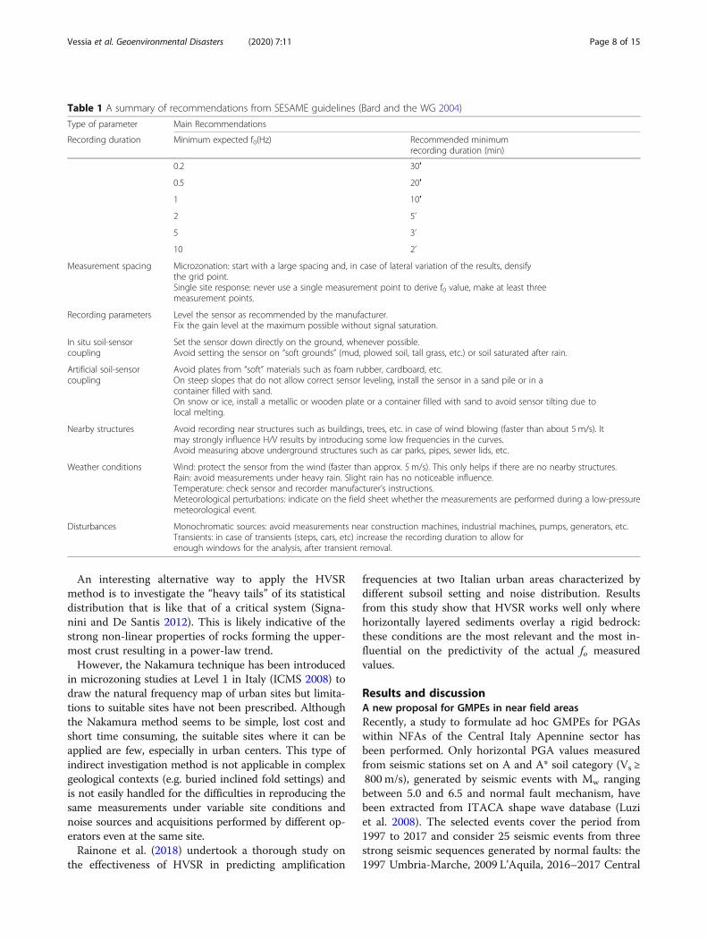
noise recording was provided by the European researchproject named SESAME (Bard and the WG 2004) thatanalyzed the possible drawbacks of the simple model in-troduced by the Nakamura method and issued guide-lines that offer important recommendations regardingthe places where the method can be successfully used inurbanized areas. The given recommendations are basedon a rather strict set of criteria, that are essentially com-posed of (1) experimental conditions and (2) criteria forgaining reliable results (Table 1).As can be seen from Table 1, the recommendations

are focused on the weather conditions that influence thequality of the noise measurements and they highlight theneed to record at distance from structures, trees, slopesbecause all these items affect the records. Unfortunately,it is not possible to quantify the minimum distance fromthe structure where the influence is negligible, as thisdistance depends on too many external factors (structuretype, wind strength, soil type, etc.). Furthermore, relatedto the measurement spacing, SESAME guidelines sug-gest to never use a single measurement point to derive f0value, make at least three measurement points. This lat-ter advice is often disregarded.

Fig. 5 Horizontal and vertical PGA values recorded within the first20 km epicenter distance during 1) 22 February 2011 Christchurchearthquake (6.3 Mw) (square) and 2) 21 June 2013 Fivizzanoearthquake (5.1 Mw) (triangle)

Vessia et al. Geoenvironmental Disasters (2020) 7:11 Page 7 of 15

An interesting alternative way to apply the HVSRmethod is to investigate the “heavy tails” of its statisticaldistribution that is like that of a critical system (Signa-nini and De Santis 2012). This is likely indicative of thestrong non-linear properties of rocks forming the upper-most crust resulting in a power-law trend.However, the Nakamura technique has been introduced

in microzoning studies at Level 1 in Italy (ICMS 2008) todraw the natural frequency map of urban sites but limita-tions to suitable sites have not been prescribed. Althoughthe Nakamura method seems to be simple, lost cost andshort time consuming, the suitable sites where it can beapplied are few, especially in urban centers. This type ofindirect investigation method is not applicable in complexgeological contexts (e.g. buried inclined fold settings) andis not easily handled for the difficulties in reproducing thesame measurements under variable site conditions andnoise sources and acquisitions performed by different op-erators even at the same site.Rainone et al. (2018) undertook a thorough study on

the effectiveness of HVSR in predicting amplification

frequencies at two Italian urban areas characterized bydifferent subsoil setting and noise distribution. Resultsfrom this study show that HVSR works well only wherehorizontally layered sediments overlay a rigid bedrock:these conditions are the most relevant and the most in-fluential on the predictivity of the actual fo measuredvalues.

Results and discussionA new proposal for GMPEs in near field areasRecently, a study to formulate ad hoc GMPEs for PGAswithin NFAs of the Central Italy Apennine sector hasbeen performed. Only horizontal PGA values measuredfrom seismic stations set on A and A* soil category (Vs ≥800 m/s), generated by seismic events with Mw rangingbetween 5.0 and 6.5 and normal fault mechanism, havebeen extracted from ITACA shape wave database (Luziet al. 2008). The selected events cover the period from1997 to 2017 and consider 25 seismic events from threestrong seismic sequences generated by normal faults: the1997 Umbria-Marche, 2009 L’Aquila, 2016–2017 Central

Table 1 A summary of recommendations from SESAME guidelines (Bard and the WG 2004)

Type of parameter Main Recommendations

Recording duration Minimum expected f0(Hz) Recommended minimumrecording duration (min)

0.2 30′

0.5 20′

1 10′

2 5’

5 3’

10 2’

Measurement spacing Microzonation: start with a large spacing and, in case of lateral variation of the results, densifythe grid point.Single site response: never use a single measurement point to derive f0 value, make at least threemeasurement points.

Recording parameters Level the sensor as recommended by the manufacturer.Fix the gain level at the maximum possible without signal saturation.

In situ soil-sensorcoupling

Set the sensor down directly on the ground, whenever possible.Avoid setting the sensor on “soft grounds” (mud, plowed soil, tall grass, etc.) or soil saturated after rain.

Artificial soil-sensorcoupling

Avoid plates from “soft” materials such as foam rubber, cardboard, etc.On steep slopes that do not allow correct sensor leveling, install the sensor in a sand pile or in acontainer filled with sand.On snow or ice, install a metallic or wooden plate or a container filled with sand to avoid sensor tilting due tolocal melting.

Nearby structures Avoid recording near structures such as buildings, trees, etc. in case of wind blowing (faster than about 5 m/s). Itmay strongly influence H/V results by introducing some low frequencies in the curves.Avoid measuring above underground structures such as car parks, pipes, sewer lids, etc.

Weather conditions Wind: protect the sensor from the wind (faster than approx. 5 m/s). This only helps if there are no nearby structures.Rain: avoid measurements under heavy rain. Slight rain has no noticeable influence.Temperature: check sensor and recorder manufacturer’s instructions.Meteorological perturbations: indicate on the field sheet whether the measurements are performed during a low-pressuremeteorological event.

Disturbances Monochromatic sources: avoid measurements near construction machines, industrial machines, pumps, generators, etc.Transients: in case of transients (steps, cars, etc) increase the recording duration to allow forenough windows for the analysis, after transient removal.

Vessia et al. Geoenvironmental Disasters (2020) 7:11 Page 8 of 15

Italy. The studied source area is a quadrant whose edges’coordinates are (43.5°, 12.3°) and (42.2°, 13.6°) in decimaldegrees. The PGA measures within the first 35 km fromthe seismic source have been taken into account. Thehypocentral distance has been used to define the sourceto site distance. Two GMPEs within the first 35 km havebeen drawn for two ranges of moment magnitude: 5 ≤Mw1 < 5.5 and 5.5 ≤Mw2 ≤ 6.5. These ranges representthe injurious magnitudes of the Italian moderately-highmagnitude earthquakes (Fig. 6). As can be noted fromFig. 6 the PGA values seem not to be highly different inthe two magnitude ranges and they do not show a cleartrend with the hypocentral distance. Thus, these twodatasets have been kept distinct and a box and whiskerplot has been used to calculate their medians, quartiles,and interquartile distance.Figure 7a, b show the two datasets with a different

number of bins of hypocentral distance: it is due to thecircumstance that for higher magnitudes (Fig. 7b) the

seismic stations within the first 10 km are that few thatcannot be considered a distinct bin. Thus, through Fig.7a, b the outliers are evidenced and eliminated. Thenthe 95th percentiles of the PGAs within each bin of thetwo datasets have been calculated. The mean value ofthe preceding percentiles has been considered as therepresentative constant value of the first 30 km of thehypocentral distance: 0.27 g for 5 ≤Mw1 < 5.5 and 0.37 gfor 5.5 ≤Mw2 ≤ 6.5. It is worthy to be noted that this pro-posal is related to the PGA values at the rigid ground tobe used in microzonation studies at the sites located inthe Central Italy Apennine sector within the first 30 kmhypocentral distance and in the two ranges of magni-tudes of moderately high earthquakes. The disaggrega-tion pairs at each site within NFAs can be determinedaccording to the Ingv study issued at the website: esse1.mi.ingv.it. Then, to select the reference PGA can be usedthe abovementioned method and the two values foundby this study. Further studies must be accomplished to

Fig. 6 Datasets of PGA values recorded at NFAs in the Central Italy Apennine Sector from 1997 to 2017 divided into two ranges of Mw: a 5≤Mw1 < 5.5; b 5.5≤Mw2 ≤ 6.5

Vessia et al. Geoenvironmental Disasters (2020) 7:11 Page 9 of 15

characterize the PGA of different seismic regions withinItalian territory. The same proposed approach or severalother proposals can be conceived and applied worldwidewithin the NFAs taking into account that the surficialsoil response there is not dependent on the distancefrom the source but it is much more dependent on thenon-linearity of the soil response combined with thecomplex geological conditions that cannot be easilymodelled.

HVSR measurements addressed in the Aterno ValleyThe seismic characterization of surface geology by meansof microtremors was introduced by ICMS (2008) and itwas then applied in the aftermath of the 2009 L’Aquilaearthquake. Many research groups started to record ambi-ent vibrations and process them through Nakamura’smethod ignoring, in details, the surface geology of eachtesting point. At Villa Sant’Angelo and Tussillo sites

(falling into the Macroarea 6 of the Aterno Valley namedL’Aquila crater), we performed several microtremors ac-quisitions at one station through two devices: Trominoand DAQLink III. The following acquisition parametershave been used: (1) time windows longer than 30′; (2) thesampling frequency higher than 125 Hz; (3) the samplingtime lower than 8ms. Furthermore, Fast Fourier Trans-form FFT has been used to calculate the ratio H/V. Fi-nally, the spectral smoothing has been performed bymeans of the Konno-Ohmachi smoothing window. TheHVSR values have been calculated for each sub-windowsof 20s, then the mean and the standard deviation of all ra-tios have been calculated and plotted. Further details onthe technical aspects of the acquisitions by both devicescan be found in Vessia et al. (2016).Figure 8a shows the HVSR measurements acquired at

two neighboring points in Tussillo center, where geo-logical characters were similar, by two research groups:T1 (the writing authors) and M5 (the Italian Departmentof Civil Protection DPC). These acquisitions have beendone by the Tromino equipment. As can be noted, thetwo plots are different: T1 evidences peaks at 2.5 Hz and8Hz; on the contrary, the M5 shows the main peak at 2Hz and minor peaks at 10-20 Hz, 40Hz and 55Hz. In thepresence of these peaks, the operator would select themost representative one: of course, this selection is highlysubjective although the SESAME rules suggest to take intoaccount the highest peaks, such as 2 Hz in both cases (T1and M5) and disregard the peaks higher than 20Hz.On the contrary, Fig. 8b shows the HVSRs measured

at two nearby points on a different type of ground typecompared with the previous points: T5 (the writing au-thors) and S4 (DPC group).In this latter case, the two plots show an evident peak

at 2 Hz although the peak amplitude is double at T5with respect to S4. This difference could be due to thepresence of disregarded Love waves that do not havevertical components contributing to the amplification ofthe horizontal components.Figure 9a, b compare HVSR measured at NE of T5, at

Villa Sant’Angelo historical center. In this case, the sig-nals are recorded by two devices used by us: the Tro-mino and the DAQLink devices. As can be seen, theyshow similar peaks although no unique peak values canbe drawn from each HVSR. In this case, the operatorchoices can affect the results in terms of the natural fre-quency of the site. However, the SESAME rule of threeacquisitions at 3 different points to assess HVSR couldbe useful to get to a robust assessment of fo.Another weak point in the calculation of the amplified

frequency f0 is the systematic differences in calculatedamplified frequencies coming from the noise measure-ments, that induce very small deformation in soil depositsand f0 drawn from the weak motion tails of the strong

Fig. 7 Box and whistler plots of the two datasets of PGA valuesrecorded at NFAs in the Central Italy Apennine Sector from 1997 to2017 divided into two ranges of Mw: a 5 ≤Mw1 < 5.5; b 5.5≤Mw1 ≤6.5. The bins of hypocentral distance are: a) 1(0–9.95 km), 2(10–19.95km), 3(20–29.95 km); b) 1(10–19.95 km), 2(20–29.95 km). The voidcircles are the outliers identified by the box and whistler method

Vessia et al. Geoenvironmental Disasters (2020) 7:11 Page 10 of 15

motion signals generated by the strong motion events atthe site that cause medium to large deformation levels inthe ground. From our experience, the f0 drawn from noisemeasurements are rarely confirmed by amplified frequen-cies from actual records. From the field experience, theamplified frequencies f0 have been measured through the

HVSR function from the noise tracks acquired at the Tus-sillo site, at the point T1 and the weak motion tails of aseismic event recorded on July 7, 2009, at 10:15 local timeat the same site.Figure 10 shows the HVSR functions. It is easy to no-

tice that the calculated f0 related to the noise (Fig. 10a)

Fig. 8 a H/V measurements at two neighbor points at Tussillo center: T1 (this study) and M5 (DPC). b H/V measurements performed by theTromino at T5 (this study) and at S4 (DPC) under similar ground conditions

Vessia et al. Geoenvironmental Disasters (2020) 7:11 Page 11 of 15

is shown at 8 Hz whereas and the one related to theweak motion (Fig. 10b) is calculated at 2 Hz: the peakfrequencies do not match and the weak tail, after thestrong motion excitation shows a lower amplificationfrequency due to the non-linear response of the soilcompared to the peak related to the noise measures.These results have been confirmed by other comparisonsaccomplished in several other places within the AternoValley (Vessia et al. 2016).Finally, from the abovementioned experiences, three

issues can be pointed out: (1) Nakamura’s method oftenprovides more than one peak corresponding to differentnatural frequencies; (2) the peaks are heavily affected bymany external factors, especially in urban areas, that arenot easy to be disregarded by filtering the measure-ments; (3) the peaks in HVSR functions are not com-monly related to both weak and strong motion amplifiedfrequencies.

Thus, the use of the noise measurements in microzon-ing activities to derive the bedrock depth should be dis-couraged especially when the geological conditions ofthe site are not known, such as the shear wave velocityprofile of the soil deposits up to the bedrock depth. Inaddition, the amplified frequency of the site should bedetermined through more than one measurement, ac-cording to the SESAME rules, in order to check the pos-sible differences induced by the different time of the dayand weather conditions at the site. However, the ampli-fied frequency measured at a very low deformation levelis modified at medium and large deformations inducedduring the strong and even weak motion seismic events.Thus the calculation of the f0 from noise measures canonly be used to determine the bedrock depth throughEq. (3) but the shear wave velocity profile is needed aswell as the buried geological conditions to guarantee theapplicability of the Nakamura method.

Fig. 9 Noise measurements at Villa Sant’Angelo center by a the Tromino device; b the DAQLink device

Vessia et al. Geoenvironmental Disasters (2020) 7:11 Page 12 of 15

Fig. 10 HVSR function measured at the T1 site, at Tussillo site (see Fig. 8) from: a the noise measurements; b the weak motion tail of a seismicevent recorded on 7 July 2009, at 10:15 local time

Vessia et al. Geoenvironmental Disasters (2020) 7:11 Page 13 of 15

ConclusionsIn this paper two weak points in microzoning studieshave been discussed starting from the authors’ experi-ence in microzonation in Italy, that is: (a) the lack ofpredictivity of GMPEs of PGA measurements in NFAsand (b) the ability of noise measurements to capture theamplified frequency at site even in a complex geologicalconditions. Throughout the paper, some past experi-ences of microzoning activity by the present authors arediscussed and two proposals have neem put forward. Onone hand, concerning the GMPEs of PGAs according tothe reference seismic hazard assessment performed inItaly, the need for specific GMPE values in NFAs havebeen highlighted by several scientists. Here, the proposalof using the 95 percentile of the scattered values re-corded within the first 30 km from the hypocentral dis-tance has been provided for the Central Italy ApennineSector. These values have been drawn from the ITACAdatabase limited to seismic events ranging from 5 to 6.5Mw occurred from 1997 to 2017. On the other hand,after a large experience gained in the noise measure-ments recorded in the Aterno Valey after the 2009L’Aquila earthquake, it can be concluding that the noisemeasurements are not inherently repeatable, thus at leasttwo or three measurements, according to the SESAMEguidelines (this represents the European standard to per-form ambient vibration measurements) must be re-quested to calculate the f0 by means of Nakamura’smethod. Although noise measurements can provide rele-vant differences in amplified frequencies according tothe operator or the weather conditions, following theSESAME rules guarantee both technical standards to anunregulated geophysical technique that relies on a sim-ple buried geological model of horizontally layered soildeposits. This model, when not applicable, can make theHVSR function from noise measurements totally mis-leading. Thus, even at level 1 microzoning studies, theuse of direct and indirect measures is needed in order toconfirm the layered planar setting of the subsurface geo-lithological model and measuring shear wave velocityprofiles to enable a robust prediction of the bedrockdepth by means of the amplified frequency f0 estimation.Finally, when the noise measurements are compared

with the weak motion tails of actual seismic events, theyshow different amplified ranges of frequencies. Accord-ingly, it must be kept in mind that soil behavior isstrain-dependent: this means that their natural frequen-cies at small strain levels (microtremors) differ from theones at medium strain level (weak motions) and at highstrain level (strong motions). Then, depending on thepurpose of the natural frequency measurement, differentstrain levels will be investigated to do an adequatecharacterization of the site response under seismicexcitation.

AbbreviationsAI: Arias Intensity; CAV: Cumulative Absolute Velocity; FA: Amplification factorin terms of accelerations; FV: Amplification factor in terms of velocities;GMPE: Ground Motion Prediction Equation; HVSR: Horizontal to VerticalSpectral Ratio; MCS: Mercalli-Cancani-Sieberg Intensity Scale;MM: Microzoning map; NFA: Near Field Area; PGA: Peak Ground Acceleration;PSA: Peak Spectral Acceleration; PSHA: Probabilistic Seismic HazardAssessment; RSH: Reference Seismic Hazard

AcknowledgmentsThe authors are grateful to Prof. Patrizio Signanini who gave precioussuggestions during the paper preparation and inspired several discussionson the effects of inefficient microzonation studies on people’s daily lifequality in near field seismic areas.

Authors’ contributionsTo this study, GV was responsible for the state of the art research(Introduction and Methods section) and the Results section related to 3.1paragraph; MLR and ADS were responsible for the geophysical campaignand the Results section discussing results; GE acquired some ambient noiserecords and was responsible for the figures. All the authors contributedtogether to the writing of the manuscript. The author(s) read and approvedthe final manuscript.

FundingNot applicable.

Availability of data and materialsNot applicable.

Competing interestsThe authors declare that they have no competing interests.

Author details1Department of Engineering and Geology, University “G.d’Annunzio” ofChieti-Pescara, Via dei Vestini 31, 66013 Chieti, Scalo (CH), Italy. 2IstitutoNazionale di Geofisica e Vulcanologia (INGV), Via di Vigna Murata, 605, 00143Rome, Italy.

Received: 11 August 2019 Accepted: 26 February 2020

ReferencesAbrahamson NA, Silva WJ (2008) Summary of the Abrahamson & Silva NGA

ground motion relations. Earthquake Spectra 24(1):67–97Bard P-Y and the WG (2004) SESAME European research project WP12 –

Deliverable D23.12. Guidelines for the implementation of the H/V spectralratio technique on ambient vibrations measurements, processing andinterpretation. http://sesame-fp5.obs.ujf-grenoble.fr/index.htm

Bergamaschi F, Cultrera G, Luzi L, Azzara RM, Ameri G, Augliera P, Bordoni P, CaraF, Cogliano R, D’alema E, Di Giacomo D, Di Giulio G, Fodarella A,Franceschina G, Galadini F, Gallipoli MR, Gori S, Harabaglia P, Ladina C, LovatiS, Marzorati S, Massa M, Milana G, Mucciarelli M, Pacor F, Parolai S, Picozzi M,Pilz M, Pucillo S, Puglia R, Riccio G, Sobiesiak M (2011) Evaluation of siteeffects in the Aterno river valley (Central Italy) from aftershocks of the 2009L’Aquila earthquake. Bull Earthq Eng 9:697–715

Bindi D, Massa M, Luzi L, Ameri G, Pacor F, Puglia R, Augliera P (2014) Pan-European ground-motion prediction equations for the average horizontalcomponent of PGA, PGV and 5%-damped PSA at spectral periods up to 3.0 susing the RESORCE dataset. Bull Earthq Eng 12:391–430. https://doi.org/10.1007/s10518-013-9525-5

Bindi D, Pacor F, Luzi L, Puglia R, Massa M, Ameri G, Paolucci R (2011) Ground-motion prediction equations derived from the Italian strong motiondatabase. Bull Earthq Eng 9(6):1899–1920. https://doi.org/10.1007/s10518-011-9313-z

Boncio P, Amoroso S, Vessia G, Francescone M, Nardone M, Monaco P, FamianiD, Di Naccio D, Mercuri A, Manuel MR, Galadini F, Milana G (2018) Evaluationof liquefaction potential in an intermountain quaternary lacustrine basin(Fucino basin, Central Italy): implications for seismic microzonation mapping.Bull Earthq Eng 16(1):91–111. https://doi.org/10.1007/s10518-017-0201-z

Boore DM (2004) Can site response be predicted? J Earthq Eng 8(1):1–41

Vessia et al. Geoenvironmental Disasters (2020) 7:11 Page 14 of 15

Boore DM (2013) What Do Ground-Motion Prediction Equations Tell Us AboutMotions Near Faults?. 40th Workshop of the International School ofGeophysics on properties and processes of crustal fault zones, EttoreMajorana Foundation and Centre for Scientific Culture, Erice, Sicily, Italy, May18–24 (invited talk)

Boore DM (2014a) What do data used to develop ground-motion predictionequations tell us about motions near faults? Pure Appl Geophys 171:3023–3043

Boore DM (2014b) The 2014 William B. Joyner lecture: ground-motion predictionequations: past, present, and future. New Mexico State University, Las Cruces,New Mexico, April 17

Boschi E, Favali F, Frugoni F, Scalera G, Smriglio G (1995) Massima IntensitàMacrosismica risentita in Italia (Map, scale 1:1.500.000)

Bradley BA, Cubrinovski M (2011) Near-source strong ground motions observedin the 22 February 2011 Christchurch earthquake. Bull New Zealand Soc forEarthq Eng 44(4):181–194

Campbell KW, Bozorgnia Y (2012) A comparison of ground motion predictionequations for arias intensity and cumulative absolute velocity developedusing a consistent database and functional form. Earthquake Spectra 28(3):931–941. https://doi.org/10.1193/1.4000067

Cauzzi C, Faccioli E, Vanini M, Bianchini A (2014) Updated predictive equationsfor broadband (0.01–10 s) horizontal response spectra and peak groundmotions, based on a global dataset of digital acceleration records. BullEarthq Eng 13:1587–1612. https://doi.org/10.1007/s10518-014-9685-y

Cornell CA (1968) Engineering seismic risk analysis. BSSA 58(5):1583–1606Di Giulio G, Marzorati S, Bergamaschi F, Bordoni P, Cara F, D’Alema E, Ladina C,

Massa M, and il Gruppo dell’esperimento L’Aquila (2011) Local variability of theground shaking during the 2009 L’Aquila earthquake (April 6, 2009 mw 6.3): thecase study of Onna and Monticchio villages. Bull Earthq Eng 9:783–807

Faccioli E (2012) Relazioni empiriche per l’attenuazione del moto sismico delsuolo. Teaching notes

Faccioli E, Bianchini A, Villani E (2010) New ground motion prediction equationsfor T > 1 s and their influence on seismic hazard assessment. Proceedings ofthe University of Tokyo Symposium on long-period ground motion andurban disaster mitigation, March 17-18

Frankel A (1995) Mapping seismic hazard in the central and eastern UnitedStates. Seism Res Lett 66:8–21

Frankel A, Mueller C, Barnhard T, Leyendecker E, Wesson R, Harmsen S, Klein F,Perkins D, Dickman N, Hanson S, Hopper M (2000) USGS national seismichazard maps. Earthq Spectr 16:1–19

Frankel A, Mueller C, Barnhard T, Perkins D, Leyendecker E, Dickman N, Hanson S,Hopper M (1996) National seismic hazard maps. Open- file-report 96-532, U.S.G.S., Denver, p 110

Galli P, Camassi R (eds) (2009) Rapporto sugli effetti del terremoto aquilano del 6aprile 2009, Rapporto congiunto DPC-INGV, p 12 http://www.mi.ingv.it/eq/090406/quest.html

Hollenback J, Goulet CA, Boore DM (2015) Adjustment for source depth, chapter3 in NGA-east: adjustments to median ground-motion models for centraland eastern North America, PEER report 2015/08, Pacific EarthquakeEngineering Research Center

Indirizzi e criteri per la microzonazione sismica (ICMS). Dipartimento di ProtezioneCivile (DPC) e Conferenza delle Regioni e delle Province Autonome (2008).www.protezionecivile.gov.it/jcms/it/view_pub.wp?contentId=PUB1137.

Jackson D, Kagan Y (1999) Testable earthquake forecasts for 1999. Seism Res Lett70:393–403

Kempton JJ, Stewart JP (2006) Prediction equations for significant duration ofearthquake ground motions considering site and near-source effects.Earthquake Spectra 22(4):985–1013. https://doi.org/10.1193/1.2358175

Kramer SL (1996) Geotechnical earthquake engineering. Prentice-Hall, UpperSaddle River

Lanzo G, Di Capua G, Kayen RE, Kieffer DS, Button E, Biscontin G, ScasserraG, Tommasi P, Pagliaroli A, Silvestri F, d’Onofrio A, Violante C, SimonelliAL, Puglia R, Mylonakis G, Athanasopoulos G, Vlahakis V, Stewart JP(2010) Seismological and geotechnical aspects of the mw=6.3 L’Aquilaearthquake in Central Italy on 6 April 2009. Int J Geoeng Case Histories1(4):206–339

Lanzo G, Tommasi P, Ausilio A, Aversa S, Bozzoni F, Cairo R, D’Onofrio A, DuranteMG, Foti S, Giallini S, Mucciacciaro M, Pagliaroli A, Sica S, Silvestri F, Vessia G,Zimmaro P (2019) Reconnaissance of geotechnical aspects of the 2016Central Italy earthquakes. Bull Earthq Eng 17:5495–5532. https://doi.org/10.1007/s10518-018-0350-8

Luzi L, Hailemikael S, Bindi D, Pacor F, Mele F, Sabetta F (2008) ITACA (ItalianACcelerometric archive): a web portal for the dissemination of Italian strong-motion data. Seismol Res Lett 79(5):716–722. https://doi.org/10.1785/gssrl.79.5.716

Mc Guire RK (1978) FRISK: computer program for seismic risk analysis using faultsas earthquake sources. Open file report no 78-1007, U.S.G.S., Denver

Midorikawa S (2002) Importance of damage data from destructive earthquakesfor seismic microzoning. Damage distribution during the 1923 Kanto, Japan,earthquake. Ann Geophys-Italy 45(6):769–778

Miyajima M, Setiawan H, Yoshida M et al (2019) Geotechnical damage in the2018 Sulawesi earthquake, Indonesia. Geoenviron Disasters 6:6. https://doi.org/10.1186/s40677-019-0121-0

Molina S, Lindholm CD, Bungum H (2001) Probabilistic seismic hazard analysis:zoning free versus zoning methodology. B Geofis Teor Appl 42(1–2):19–39

Nakamura Y (1989) A method for dynamic characteristics estimation ofsubsurface using microtremor on the ground surface. QR Railway Tech ResInst 30(1):25–33

Paolini S, Martini G, Carpani B, Forni M, Bongiovanni G, Clemente P, Rinaldis D,Verrubbi V (2012) The may 2012 seismic sequence in Pianura PadanaEmiliana: hazard, historical seismicity and preliminary analysis ofaccelerometric records. Special issue on focus - Energia, Ambiente,Innovazione: the Pianura Padana Emiliana Earthquake 4–5(II):6–22

Paolucci R (2002) Amplification of earthquake ground motion by steeptopographic irregularities. Earthquake Eng Struc 31(10):1831–1853

Perkins D (2000) Fuzzy sources, maximum likelihood and the new methodology.In: Lapajne JK (ed) Seismicity modelling in seismic hazard mapping.Geophysical Survey of Slovenia, Ljubljana, pp 67–75

Rainone ML, D’Elia G, Vessia G, De Santis A (2018) The HVSR interpretationtechnique of ambient noise to seismic characterization of soils inheterogeneous geological contexts. Book of abstract of 36th generalassembly of the European seismological commission, ESC2018-S29-639: 428-429, 2-7 September 2018, Valletta (Malta) ISBN: 978-88-98161-12-6

Rainone ML, Vessia G, Signanini P, Greco P, Di Benedetto S (2013) Evaluating siteeffects in near field conditions for microzonation purposes: The case study ofL’Aquila earthquake 2009. (special issue on L’Aquila earthquake 2009). ItalGeotechnical J 47(3):48–68

Signanini P, Cucchi F, Frinzi U, Scotti A (1983) Esempio di microzonizzazionenell'area di Ragogna (Udine). Rendiconti della Soc Geol Italiana 4:645–653

Signanini P, De Santis A (2012) Power-law frequency distribution of H/V spectralratio of seismic signals: evidence for a critical crust. Earth Planets Space 64:49–54

Stewart JP, Boore DM, Seyhan E, Atkinson GM, M.EERI Atkinson GM (2016) NGA-West2 Equations for Predicting Vertical-Component PGA, PGV, and 5%-Damped PSA from Shallow Crustal Earthquakes show less. Earthq Spectr32(2):1005–1031. https://doi.org/10.1193/072114EQS116M

Vessia G, Parise M, Tromba G (2013) A strategy to address the task of seismicmicro-zoning in landslide-prone areas. Adv Geosci 1:1–27. https://doi.org/10.5194/adgeo-35-23-2013

Vessia G, Pisano L, Tromba G, Parise M (2017) Seismically induced slope instabilitymaps validated at an urban scale by site numerical simulations. Bull Eng GeolEnvir 76(2):457–476

Vessia G, Rainone ML, Signanini P (2016) Springer book title: “earthquakes and theirimpacts on society”, Eds. S. D’Amico, 2016 chapter 9 title: “working strategies foraddressing microzoning studies in urban areas: lessons from 2009 L'Aquilaearthquake”, 233–290, Springer international publishing Switzerland

Vessia G, Russo S, Lo Presti D (2011) A new proposal for the evaluation of theamplification coefficient due to valley effects in the simplified local seismicresponse analyses. Ital Geotechnical J 4:51–77

Vessia G, Russo S (2013) Relevant features of the valley seismic response: the casestudy of Tuscan northern Apennine sector. Bull Earthq Eng 11(5):1633–1660

Vessia G, Venisti N (2011) Liquefaction damage potential for seismic hazardevaluation in urbanized areas. Soil Dyn Earthq Eng 31:1094–1105

Woo G (1996) Kernel estimation methods for seismic hazard area sourcemodeling. Bull Seism Soc Am 86:1–10

Yagoub MM (2015) Spatio-temporal and hazard mapping of earthquake in UAE(1984–2012): remote sensing and GIS application. Geoenviron Disasters 2:13.https://doi.org/10.1186/s40677-015-0020-y

Publisher’s NoteSpringer Nature remains neutral with regard to jurisdictional claims inpublished maps and institutional affiliations.

Vessia et al. Geoenvironmental Disasters (2020) 7:11 Page 15 of 15