Lesson 5 - Polynomials - Math Blog · Lesson 5 - Polynomials ... A cubic function is a third degree...
21
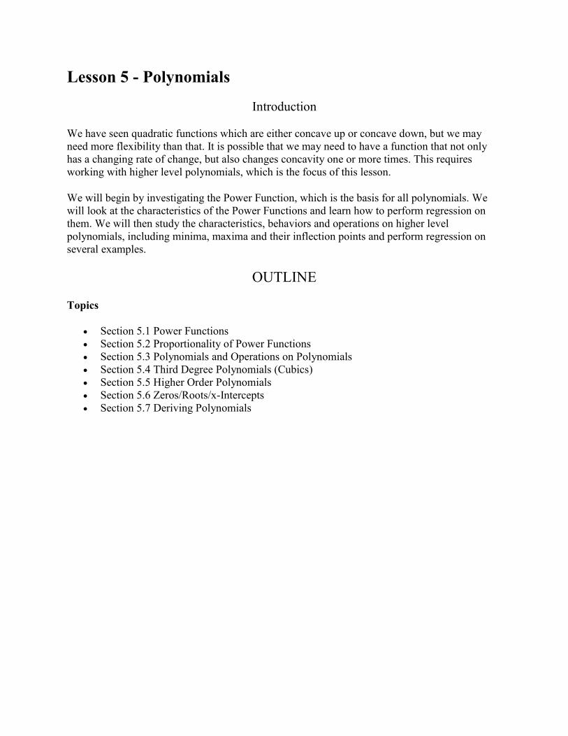
Lesson 5 - Polynomials Introduction We have seen quadratic functions which are either concave up or concave down, but we may need more flexibility than that. It is possible that we may need to have a function that not only has a changing rate of change, but also changes concavity one or more times. This requires working with higher level polynomials, which is the focus of this lesson. We will begin by investigating the Power Function, which is the basis for all polynomials. We will look at the characteristics of the Power Functions and learn how to perform regression on them. We will then study the characteristics, behaviors and operations on higher level polynomials, including minima, maxima and their inflection points and perform regression on several examples. OUTLINE Topics Section 5.1 Power Functions Section 5.2 Proportionality of Power Functions Section 5.3 Polynomials and Operations on Polynomials Section 5.4 Third Degree Polynomials (Cubics) Section 5.5 Higher Order Polynomials Section 5.6 Zeros/Roots/x-Intercepts Section 5.7 Deriving Polynomials
-
Upload
duongkhanh -
Category
Documents
-
view
218 -
download
2
Transcript of Lesson 5 - Polynomials - Math Blog · Lesson 5 - Polynomials ... A cubic function is a third degree...
Lesson 5 - Polynomials
Introduction
We have seen quadratic functions which are either concave up or concave down, but we may
need more flexibility than that. It is possible that we may need to have a function that not only
has a changing rate of change, but also changes concavity one or more times. This requires
working with higher level polynomials, which is the focus of this lesson.
We will begin by investigating the Power Function, which is the basis for all polynomials. We
will look at the characteristics of the Power Functions and learn how to perform regression on
them. We will then study the characteristics, behaviors and operations on higher level
polynomials, including minima, maxima and their inflection points and perform regression on
several examples.
OUTLINE
Topics
Section 5.1 Power Functions
Section 5.2 Proportionality of Power Functions
Section 5.3 Polynomials and Operations on Polynomials
Section 5.4 Third Degree Polynomials (Cubics)
Section 5.5 Higher Order Polynomials
Section 5.6 Zeros/Roots/x-Intercepts
Section 5.7 Deriving Polynomials
Section 5.1 - Power Functions
Before we look deeper into the definition and characteristics of the Power Function, let's take a
look at an formula you should be very familiar with,
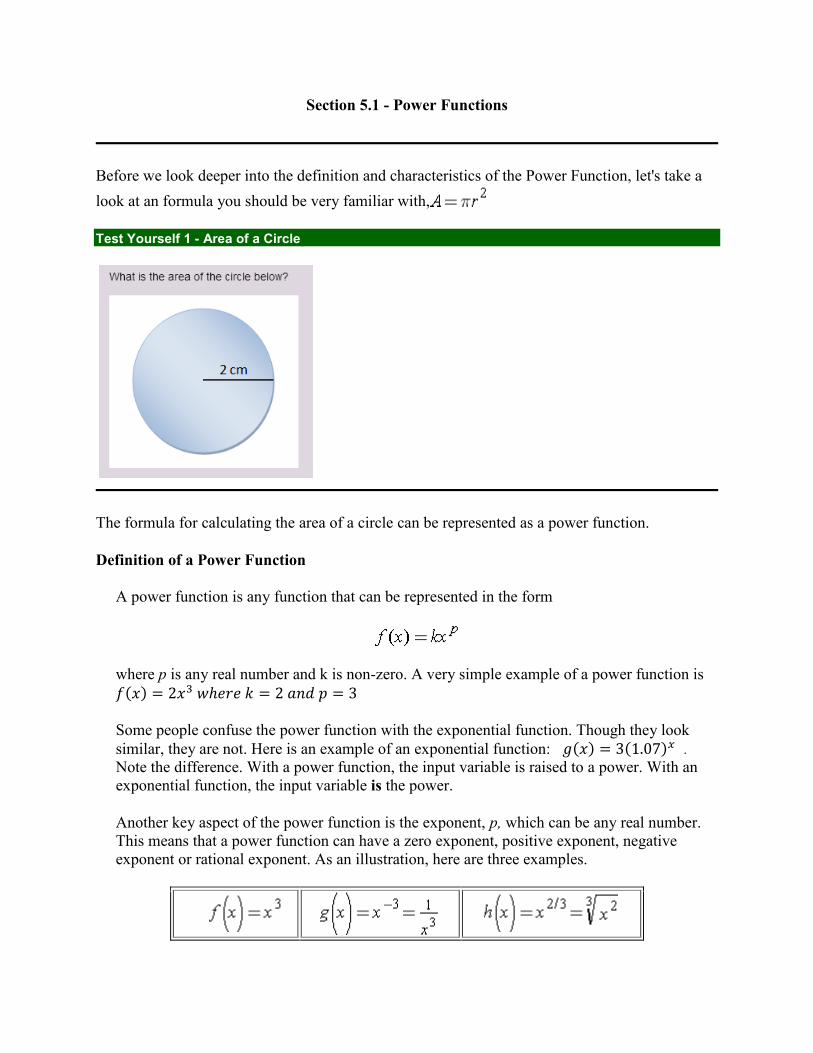
Test Yourself 1 - Area of a Circle
The formula for calculating the area of a circle can be represented as a power function.
Definition of a Power Function
A power function is any function that can be represented in the form
where p is any real number and k is non-zero. A very simple example of a power function is
( )
Some people confuse the power function with the exponential function. Though they look
similar, they are not. Here is an example of an exponential function: ( ) ( ) .
Note the difference. With a power function, the input variable is raised to a power. With an
exponential function, the input variable is the power.
Another key aspect of the power function is the exponent, p, which can be any real number.
This means that a power function can have a zero exponent, positive exponent, negative
exponent or rational exponent. As an illustration, here are three examples.

Test Yourself 2 - Power Functions
Note: We can vertically (or horizontally) scale our power function and we will still have a power
function. We can also reflect our power function over either axis and we still have a power
function. But if we shift our power function left, right, up or down, it is no longer a power
function as a requirement is that only x is raised to the p.
Characteristics of an Even Power
Function
Let's see if we can identify some
basic characteristics of power
functions. Below is a plot of
several power functions, all with
even exponents.
So we see that they are of similar
shape and are all even functions.
What about their end behavior?
We see that as , that
( ) and as , that
( ) , so using our limit
notation we have
( )
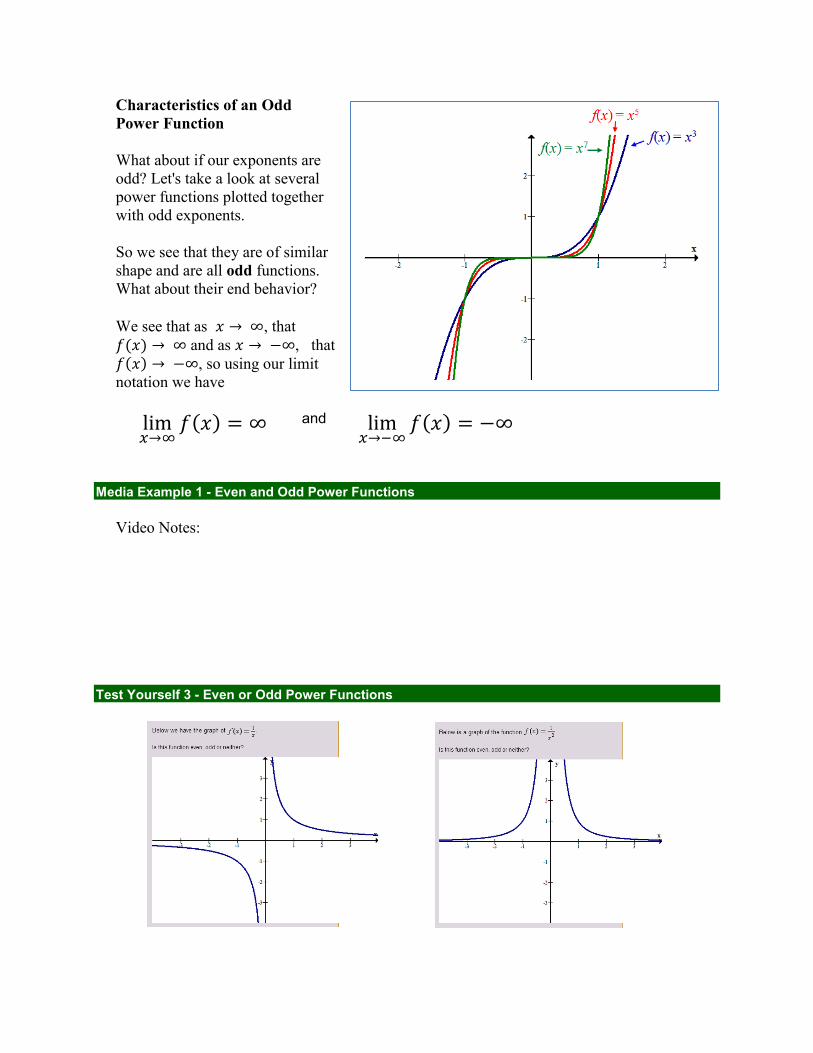
Characteristics of an Odd
Power Function
What about if our exponents are
odd? Let's take a look at several
power functions plotted together
with odd exponents.
So we see that they are of similar
shape and are all odd functions.
What about their end behavior?
We see that as , that
( ) and as , that
( ) , so using our limit
notation we have
( ) and
( )
Media Example 1 - Even and Odd Power Functions
Video Notes:
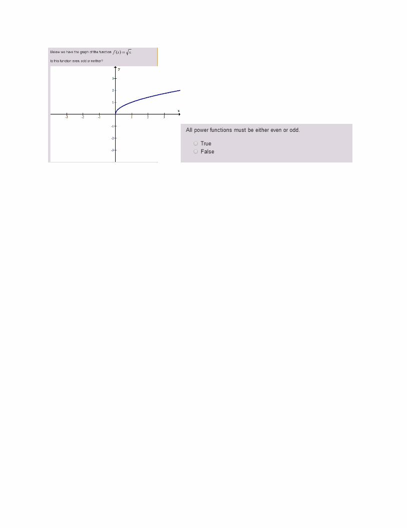
Test Yourself 3 - Even or Odd Power Functions
Section 5.2 - Proportionality of Power Functions
Power functions have some pretty important uses. A couple we will look at will be with how a
power function can be used to represent a proportional relationship and how a power function
can be used to model data.
Power Functions and Proportionality
In mathematics the term proportionality means the relationship of two variables whose ratio is
constant. For example, if you are driving at a constant speed of 25 miles per hour, we have a
proportional relationship between the time driven and the total distance. This is because our
distance is ALWAYS 25 times the number of hours driven. We could create a power function
to represent this situation.
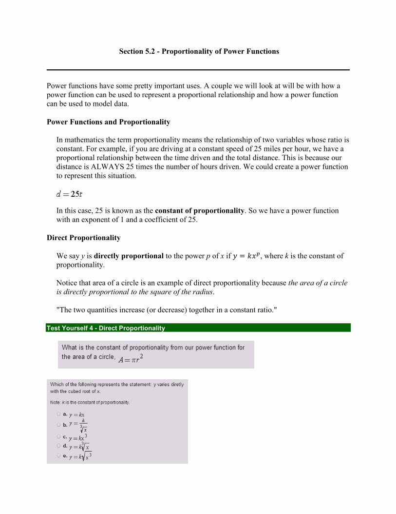
In this case, 25 is known as the constant of proportionality. So we have a power function
with an exponent of 1 and a coefficient of 25.
Direct Proportionality
We say y is directly proportional to the power p of x if , where k is the constant of
proportionality.
Notice that area of a circle is an example of direct proportionality because the area of a circle
is directly proportional to the square of the radius.
"The two quantities increase (or decrease) together in a constant ratio."
Test Yourself 4 - Direct Proportionality

Inverse Proportionality
We say y is inversely proportional to the power p of x if
where k is the constant of
proportionality.
"When one quantity increases (or decreases), the other quantity decreases (or increases), thus
they have an inverse relationship."
Test Yourself 5 - Inverse Proportionality
Let's take a look at how these appear in problems.
Media Example 2 - Direct Variation
y varies directly with x. When x = 12, y = 48. Find a function relating x and y and use it to
determine y when x = 20.
Media Example 3 - Direct Variation Application

Media Example 4 - Inverse Variation
y varies inversely with the square of x. When x = 2, y = 10. Find a function relating x and y and
use it to determine x when y is 20.
Media Example 5 - Inverse Variation Application
Worked Example 3 - Power Regression
We can do regression with power
functions just as we can do it with linear
and quadratic functions. In fact, the steps
are the same except we will choose
PwrReg when it comes time to calculate
our regression function. For example,
given the following data:
Using x=0 to be the year 1900, when we run a PwrReg, we get the following results. Use the
results to answer the questions that follow:
a=.3274 b=2.0713 r2=.9959 r=.9980
Test Yourself 6 - Power Regression
Given the Power Regression results from above, answer the following:
Section 5.3 - Polynomials and Operations on Polynomials
While power functions are nice, they are somewhat limited. It turns out when we add or subtract
power functions whose exponents are non-negative integers, we get a new class of functions
called polynomials. Polynomials have some very nice properties and offer some characteristics
that power functions are not able to.
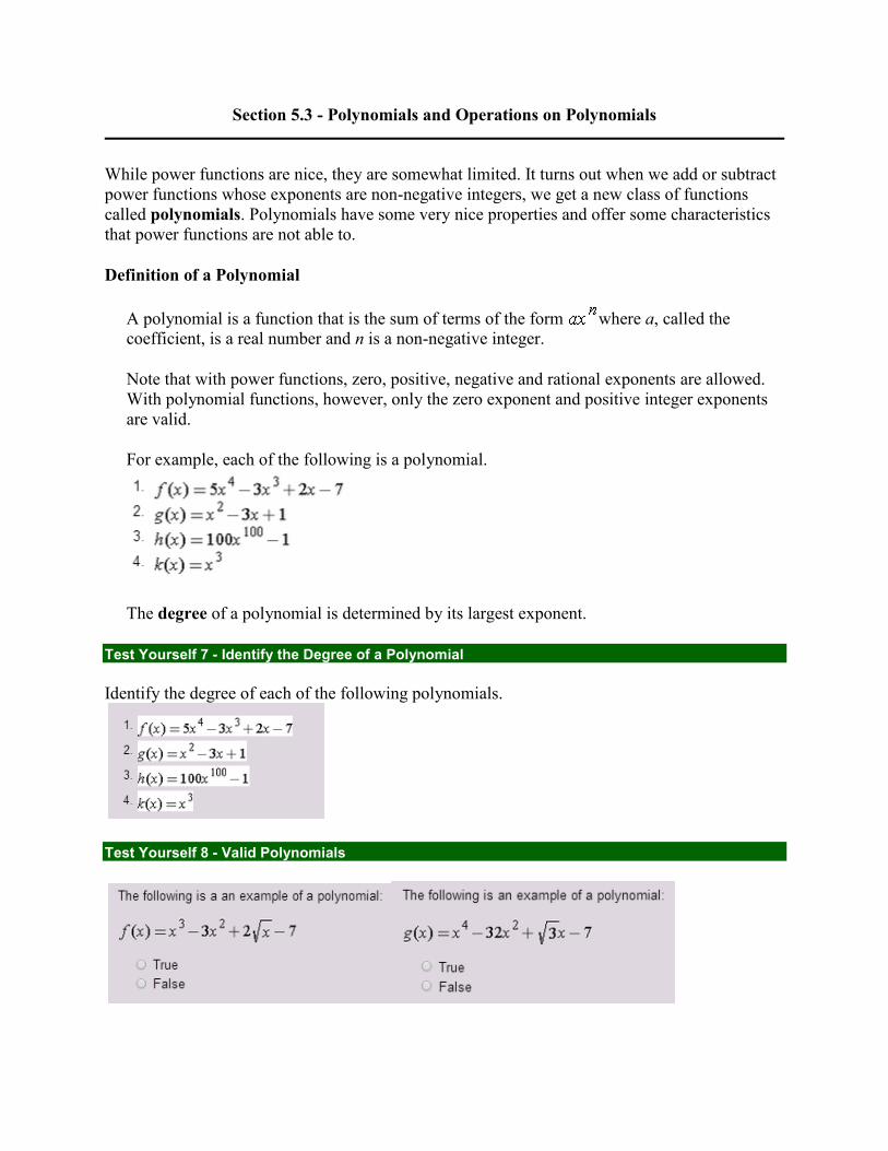
Definition of a Polynomial
A polynomial is a function that is the sum of terms of the form where a, called the
coefficient, is a real number and n is a non-negative integer.
Note that with power functions, zero, positive, negative and rational exponents are allowed.
With polynomial functions, however, only the zero exponent and positive integer exponents
are valid.
For example, each of the following is a polynomial.
The degree of a polynomial is determined by its largest exponent.
Test Yourself 7 - Identify the Degree of a Polynomial
Identify the degree of each of the following polynomials.
Test Yourself 8 - Valid Polynomials

Media Example 6 - Characteristics of Polynomials
Video Notes:
Operations on Polynomials
New polynomials can be derived by combining two or more polynomials using addition,
subtraction, multiplication and division. It's important to adhere to the properties of exponents
and order of operations to ensure the new polynomial is valid.
Media Example 7 - Polynomial Addition and Subtraction
Video Notes
Media Example 8 - Basic Polynomial Multiplication (FOIL)
Video Notes
Media Example 9 - Higher Order Polynomial Multiplication
Video Notes
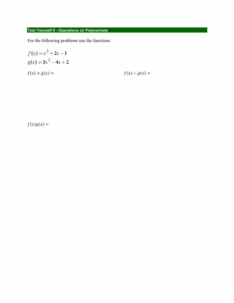
Test Yourself 9 - Operations on Polynomials
For the following problems use the functions
( ) ( ) ( ) ( )
( ) ( )

Section 5.4 - Third Degree Polynomials (Cubics)
Thus far we have looked at polynomials of degree 1 (Linear) and degree 2 (Quadratic). A
polynomial can have a much higher degree and often that can be useful when we are dealing
with situations in which the concavity changes. Let's take a look at the following situation.
Worked Example 1 - Third Degree Polynomial
The following table gives the number of Non business Chapter
11 Bankruptcies
As always, let's take a look at the data to see if we can
determine any trends.
The points do not appear linear at all. In fact, linear regression on this data set returns a
correlation coefficient of 0.3341, very low.
The points appear to be concave up at first, and then concave down towards the latter
half. To be quadratic, the model should always have the same concavity so quadratic does
not appear to be a good fit. In fact, quadratic regression yields an r² of 0.5613, again not
very good.
Thus we need a more advanced model to handle this data set. The next polynomial we come to is
a third degree, or a cubic.
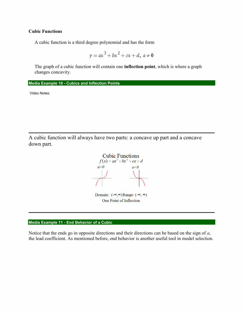
Cubic Functions
A cubic function is a third degree polynomial and has the form
The graph of a cubic function will contain one inflection point, which is where a graph
changes concavity.
Media Example 10 - Cubics and Inflection Points
Video Notes:
A cubic function will always have two parts: a concave up part and a concave
down part.
Media Example 11 - End Behavior of a Cubic
Notice that the ends go in opposite directions and their directions can be based on the sign of a,
the lead coefficient. As mentioned before, end behavior is another useful tool in model selection.

Test Yourself 10 - End Behavior of a Cubic
Worked Example 1 Continued - Cubic Regression
Now let's do cubic regression to find the model for our Non business Chapter 11 Bankruptcies
data. The calculator procedure is the same
as the previous regressions except we will
select CubicReg from the Stat-Calc menu
of regression models.
While it's not a perfect fit, it does represent
the trend of our data much better than linear
regression or quadratic regression. Also we
get an r² of 0.9822 telling us a cubic model
is a good fit.

Section 5.5 - Higher Order Polynomials
What if our concavity changes more than once? What if we have more than one inflection point?
What if it changes several times? Not to worry, we can just use a higher order polynomial.
Test Yourself 11 - Higher Order Polynomial
Examine the graph below of a fourth degree
polynomial and answer the questions that
follow.
Are you noticing a pattern between the degree of a polynomial and the number of inflection
points it can have?
Now, depending on how many inflection points we have and the end behavior, we can determine
what degree polynomial would be sufficient for our data. We would use that along with a plot of
the function with the data and the correlation coefficient to determine a polynomial model for
our data.

Polynomial Regression
Just as we did linear, quadratic, and cubic regression, higher order polynomial regression does
exist. Our calculators will only go up to fourth degree regression, QuartReg. But there are
online tools that can help if you ever find yourself in need of higher order polynomial
regression.
Xuru's Website - This site will do up to 10th degree polynomial regression
Tutorial: Data Analysis with Excel - This site will show you how to do higher order
regression in excel.
Geogebra can be used to do higher order regression using the command "Fitpoly[]"
Note: For this course the regression capabilities of your calculator will be more than enough.
Test Yourself 12 - Higher Order Polynomials

Media Example 12 - End Behavior of Polynomials
We have looked at end behavior of quadratics and cubics, now let's see what generalizations we
can make for all polynomials.
Video Notes:
Test Yourself 13 - End Behavior
Section 5.6 - Zeros/Roots/x-Intercepts
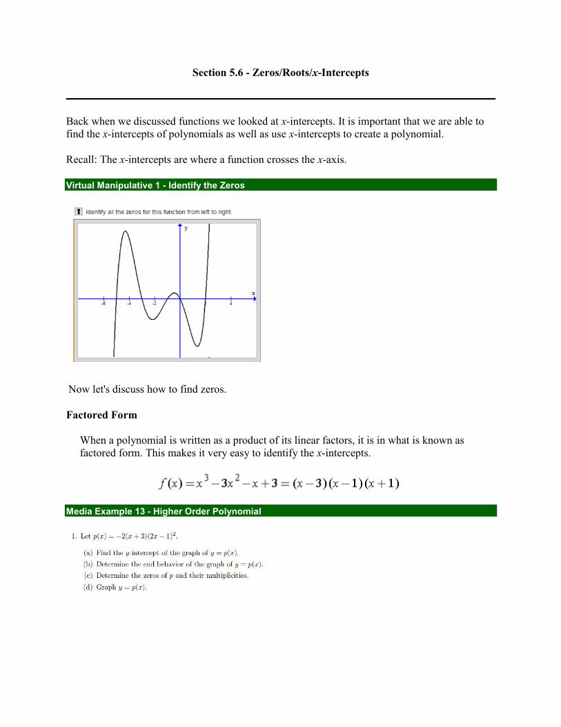
Back when we discussed functions we looked at x-intercepts. It is important that we are able to
find the x-intercepts of polynomials as well as use x-intercepts to create a polynomial.
Recall: The x-intercepts are where a function crosses the x-axis.
Virtual Manipulative 1 - Identify the Zeros
Now let's discuss how to find zeros.
Factored Form
When a polynomial is written as a product of its linear factors, it is in what is known as
factored form. This makes it very easy to identify the x-intercepts.
Media Example 13 - Higher Order Polynomial
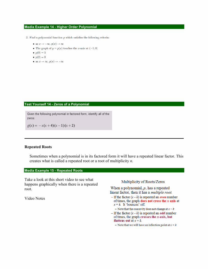
Media Example 14 - Higher Order Polynomial
Test Yourself 14 - Zeros of a Polynomial
Repeated Roots
Sometimes when a polynomial is in its factored form it will have a repeated linear factor. This
creates what is called a repeated root or a root of multiplicity n.
Media Example 15 - Repeated Roots
Take a look at this short video to see what
happens graphically when there is a repeated
root.
Video Notes
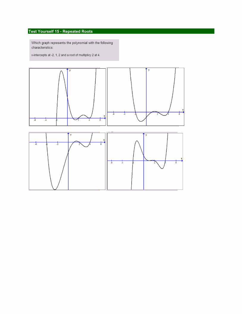
Test Yourself 15 - Repeated Roots

Section 5.7 - Deriving Polynomials
Finding an Equation for a Polynomial
The following 3 videos discuss how to use zeros and a single point to find the equation of a
polynomial.
Media Example 16 - Finding the Equation of a Polynomial given Zeros and a Single Point Example
1
Video Notes
Media Example 17 - Finding the Equation of a Polynomial given Zeros and a Single Point Example
2
Video Notes
Media Example 18 - Finding the Equation of a Polynomial given Zeros and a Single Point Example
3
Video Notes