Lesson 10: WiFi and WiMAX MAC Analysis - Springer10.1007/978-1-4614-4084...Lesson 10: WiFi and WiMAX...

Lesson 10: WiFi and WiMAX MAC Analysis Giovanni Giambene

Queuing Theory and Telecommunications: Networks and Applications 2nd edition, Springer All rights reserved

Slide supporting material

© 2013 Queuing Theory and Telecommunications: Networks and Applications – All rights reserved


WiFi Description

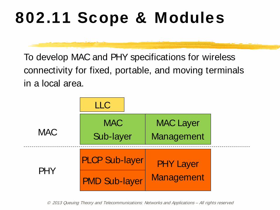
802.11 Scope & Modules

MAC Sub-layer

MAC Layer Management

PLCP Sub-layer

PMD Sub-layer

PHY Layer Management

LLC

MAC

PHY

To develop MAC and PHY specifications for wireless connectivity for fixed, portable, and moving terminals in a local area.


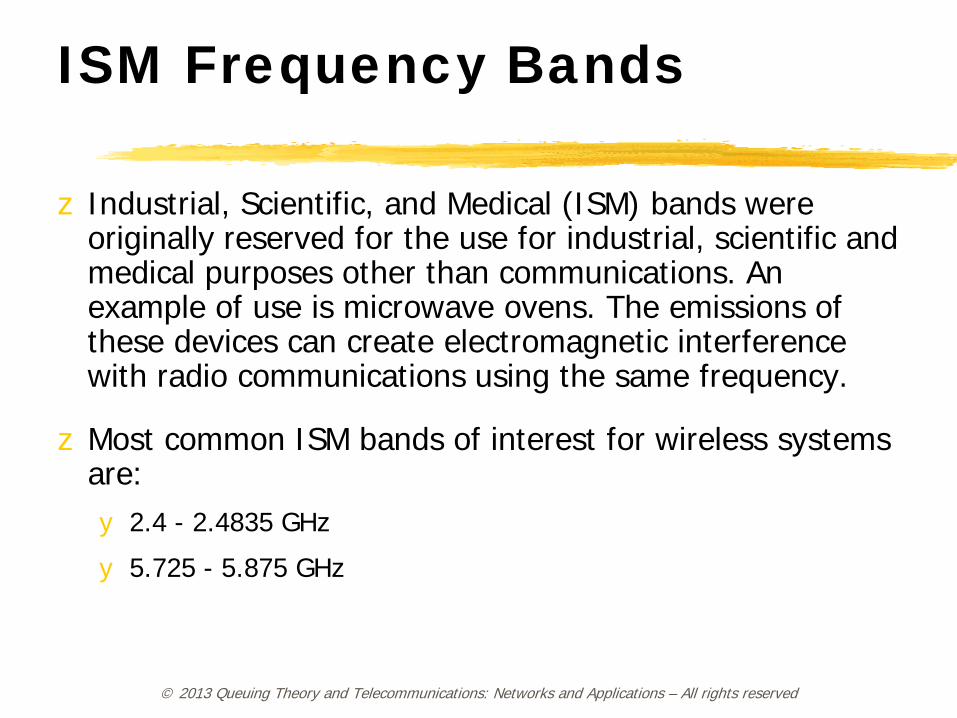
ISM Frequency Bands

z Industrial, Scientific, and Medical (ISM) bands were originally reserved for the use for industrial, scientific and medical purposes other than communications. An example of use is microwave ovens. The emissions of these devices can create electromagnetic interference with radio communications using the same frequency.

z Most common ISM bands of interest for wireless systems are:

y 2.4 - 2.4835 GHz

y 5.725 - 5.875 GHz



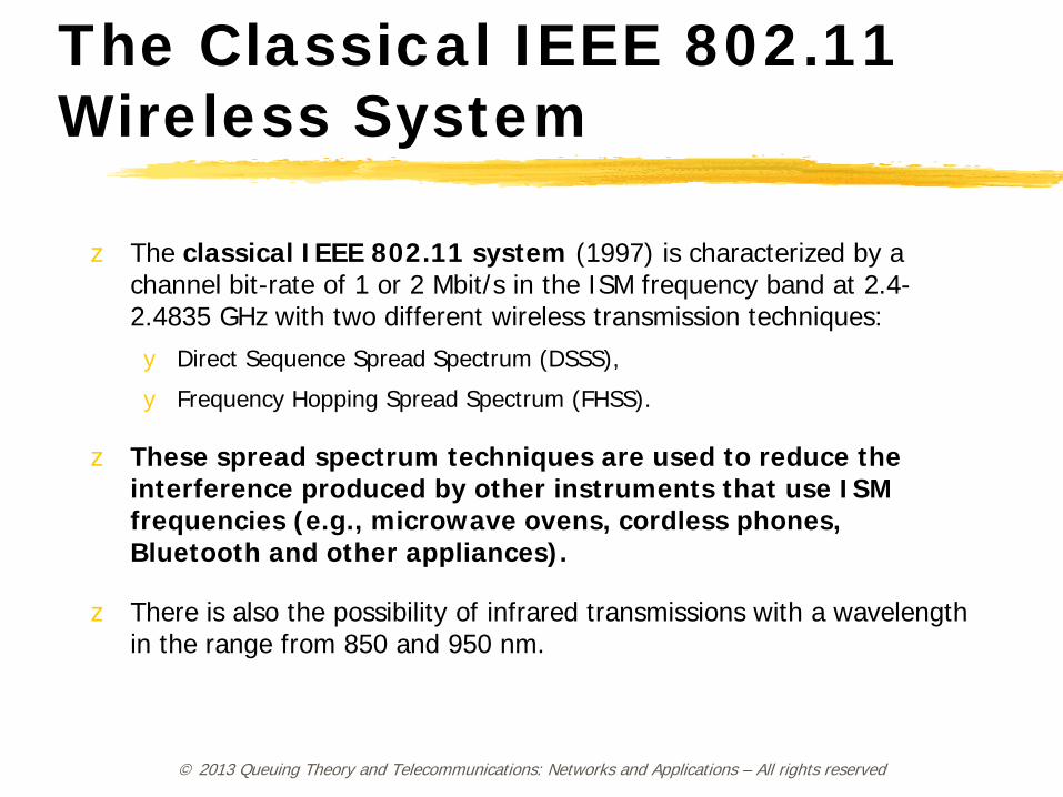
The Classical IEEE 802.11 Wireless System

z The classical IEEE 802.11 system (1997) is characterized by a channel bit-rate of 1 or 2 Mbit/s in the ISM frequency band at 2.4-2.4835 GHz with two different wireless transmission techniques:

y Direct Sequence Spread Spectrum (DSSS),

y Frequency Hopping Spread Spectrum (FHSS).

z These spread spectrum techniques are used to reduce the interference produced by other instruments that use ISM frequencies (e.g., microwave ovens, cordless phones, Bluetooth and other appliances).

z There is also the possibility of infrared transmissions with a wavelength in the range from 850 and 950 nm.


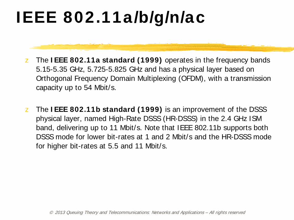
IEEE 802.11a/b/g/n/ac

z The IEEE 802.11a standard (1999) operates in the frequency bands 5.15-5.35 GHz, 5.725-5.825 GHz and has a physical layer based on Orthogonal Frequency Domain Multiplexing (OFDM), with a transmission capacity up to 54 Mbit/s.

z The IEEE 802.11b standard (1999) is an improvement of the DSSS physical layer, named High-Rate DSSS (HR-DSSS) in the 2.4 GHz ISM band, delivering up to 11 Mbit/s. Note that IEEE 802.11b supports both DSSS mode for lower bit-rates at 1 and 2 Mbit/s and the HR-DSSS mode for higher bit-rates at 5.5 and 11 Mbit/s.


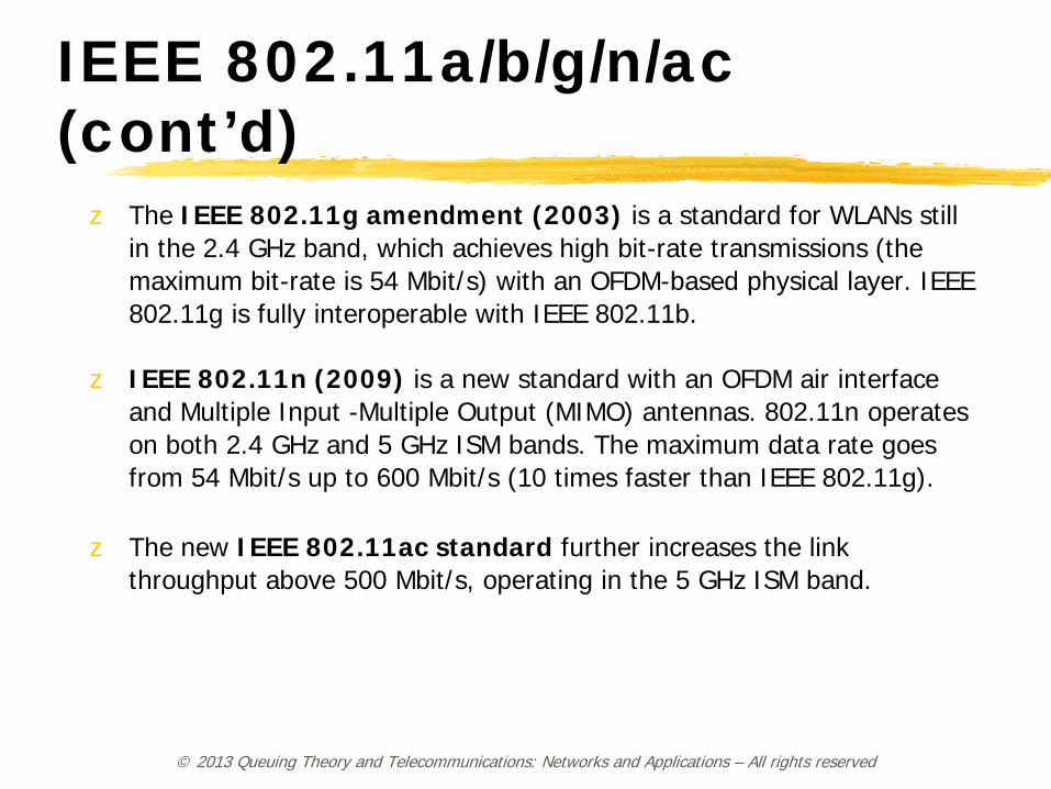
IEEE 802.11a/b/g/n/ac (cont’d)

z The IEEE 802.11g amendment (2003) is a standard for WLANs still in the 2.4 GHz band, which achieves high bit-rate transmissions (the maximum bit-rate is 54 Mbit/s) with an OFDM-based physical layer. IEEE 802.11g is fully interoperable with IEEE 802.11b.

z IEEE 802.11n (2009) is a new standard with an OFDM air interface and Multiple Input -Multiple Output (MIMO) antennas. 802.11n operates on both 2.4 GHz and 5 GHz ISM bands. The maximum data rate goes from 54 Mbit/s up to 600 Mbit/s (10 times faster than IEEE 802.11g).

z The new IEEE 802.11ac standard further increases the link throughput above 500 Mbit/s, operating in the 5 GHz ISM band.


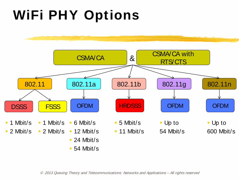
WiFi PHY Options

802.11 802.11a 802.11b 802.11g 802.11n

CSMA/CA CSMA/CA with RTS/CTS

DSSS FSSS HRDSSS OFDM OFDM OFDM

&

1 Mbit/s 2 Mbit/s

1 Mbit/s 2 Mbit/s

6 Mbit/s 12 Mbit/s 24 Mbit/s 54 Mbit/s

5 Mbit/s 11 Mbit/s

Up to 54 Mbit/s

Up to 600 Mbit/s


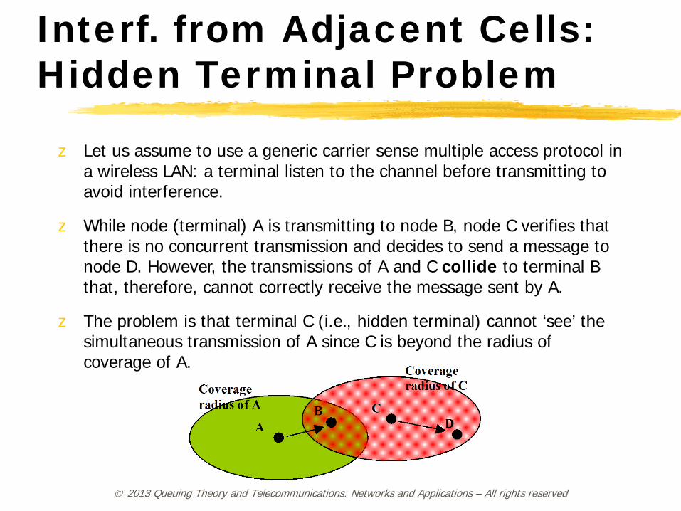
Interf. from Adjacent Cells: Hidden Terminal Problem

z Let us assume to use a generic carrier sense multiple access protocol in a wireless LAN: a terminal listen to the channel before transmitting to avoid interference.

z While node (terminal) A is transmitting to node B, node C verifies that there is no concurrent transmission and decides to send a message to node D. However, the transmissions of A and C collide to terminal B that, therefore, cannot correctly receive the message sent by A.

z The problem is that terminal C (i.e., hidden terminal) cannot ‘see’ the simultaneous transmission of A since C is beyond the radius of coverage of A.


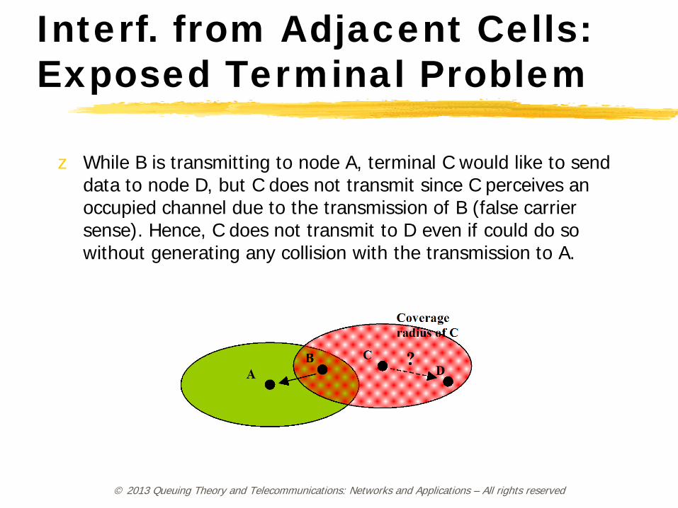
Interf. from Adjacent Cells: Exposed Terminal Problem

z While B is transmitting to node A, terminal C would like to send data to node D, but C does not transmit since C perceives an occupied channel due to the transmission of B (false carrier sense). Hence, C does not transmit to D even if could do so without generating any collision with the transmission to A.


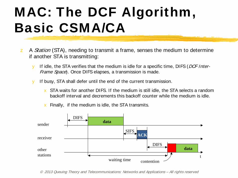
MAC: The DCF Algorithm, Basic CSMA/CA

z A Station (STA), needing to transmit a frame, senses the medium to determine if another STA is transmitting:

y If idle, the STA verifies that the medium is idle for a specific time, DIFS (DCF Inter-Frame Space). Once DIFS elapses, a transmission is made.

y If busy, STA shall defer until the end of the current transmission.

x STA waits for another DIFS. If the medium is still idle, the STA selects a random backoff interval and decrements this backoff counter while the medium is idle.

x Finally, if the medium is idle, the STA transmits.

t

SIFS

DIFS

data

ACK

waiting time

other stations

receiver

sender data

DIFS

contention


DCF Algorithm: Carrier Sensing

z In IEEE 802.11, carrier sensing is needed to determine if the medium is available. There are two methods:

y A physical carrier-sense function is provided by the PHY layer and depends on the medium and modulation used.

y A virtual carrier-sense mechanism is provided by the Network Allocation Vector (NAV), a ‘parameter’ managed by the MAC layer.

z The channel is busy if one of the two above mechanisms indicate it to be.

z If a terminal experiences a packet collision, the backoff window is doubled at the next attempt.


IEEE 802.11e: Enhanced MAC for QoS Support in WiFi

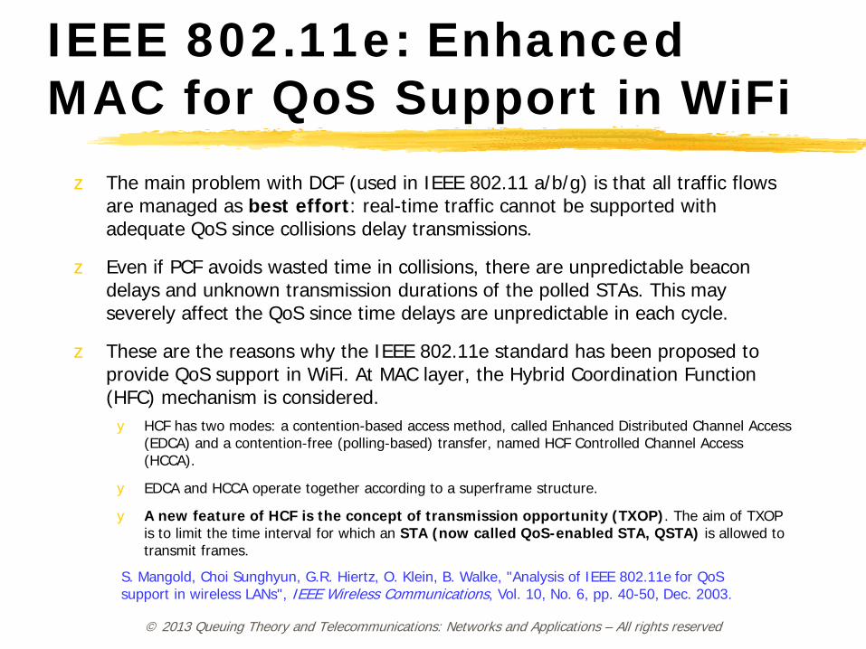
z The main problem with DCF (used in IEEE 802.11 a/b/g) is that all traffic flows are managed as best effort: real-time traffic cannot be supported with adequate QoS since collisions delay transmissions.

z Even if PCF avoids wasted time in collisions, there are unpredictable beacon delays and unknown transmission durations of the polled STAs. This may severely affect the QoS since time delays are unpredictable in each cycle.

z These are the reasons why the IEEE 802.11e standard has been proposed to provide QoS support in WiFi. At MAC layer, the Hybrid Coordination Function (HFC) mechanism is considered.

y HCF has two modes: a contention-based access method, called Enhanced Distributed Channel Access (EDCA) and a contention-free (polling-based) transfer, named HCF Controlled Channel Access (HCCA).

y EDCA and HCCA operate together according to a superframe structure.

y A new feature of HCF is the concept of transmission opportunity (TXOP). The aim of TXOP is to limit the time interval for which an STA (now called QoS-enabled STA, QSTA) is allowed to transmit frames.

S. Mangold, Choi Sunghyun, G.R. Hiertz, O. Klein, B. Walke, "Analysis of IEEE 802.11e for QoS support in wireless LANs", IEEE Wireless Communications, Vol. 10, No. 6, pp. 40-50, Dec. 2003.


IEEE 802.11e: Enhanced MAC for QoS Support (cont’d)

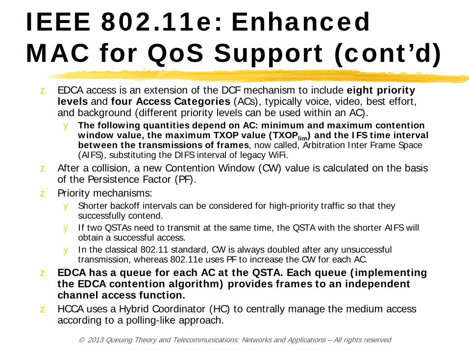
z EDCA access is an extension of the DCF mechanism to include eight priority levels and four Access Categories (ACs), typically voice, video, best effort, and background (different priority levels can be used within an AC).

y The following quantities depend on AC: minimum and maximum contention window value, the maximum TXOP value (TXOPlim) and the IFS time interval between the transmissions of frames, now called, Arbitration Inter Frame Space (AIFS), substituting the DIFS interval of legacy WiFi.

z After a collision, a new Contention Window (CW) value is calculated on the basis of the Persistence Factor (PF).

z Priority mechanisms: y Shorter backoff intervals can be considered for high-priority traffic so that they

successfully contend. y If two QSTAs need to transmit at the same time, the QSTA with the shorter AIFS will

obtain a successful access. y In the classical 802.11 standard, CW is always doubled after any unsuccessful

transmission, whereas 802.11e uses PF to increase the CW for each AC. z EDCA has a queue for each AC at the QSTA. Each queue (implementing

the EDCA contention algorithm) provides frames to an independent channel access function.

z HCCA uses a Hybrid Coordinator (HC) to centrally manage the medium access according to a polling-like approach.


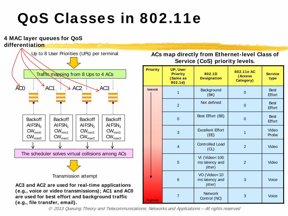
QoS Classes in 802.11e

Priority UP, User Priority

(Same as 802.1d)

802.1D Designation

802.11e AC (Access

Category)

Service type

lowest

highest

1 Background (BK) 0 Best

Effort

2 Not defined

0 Best

Effort

0 Best Effort (BE)

0 Best

Effort

3 Excellent Effort (EE) 1 Video

Probe

4 Controlled Load (CL) 2 Video

5 VI (Video<100 ms latency and

jitter) 2 Video

6 VO (Video<10 ms latency and

jitter) 3 Voice

7 Network Control (NC) 3 Voice

AC3 and AC2 are used for real-time applications (e.g., voice or video transmissions); AC1 and AC0 are used for best effort and background traffic (e.g., file transfer, email).

4 MAC layer queues for QoS differentiation

ACs map directly from Ethernet-level Class of Service (CoS) priority levels.

AC0 AC1 AC2 AC3

Backoff AIFSN0 CWmin0 CWmax0




Traffic mapping from 8 Ups to 4 ACs

Up to 8 User Priorities (UPs) per terminal

The scheduler solves virtual collisions among ACs

Transmission attempt


Parameters for EDCA of IEEE 802.11e

z The appropriate selection of the AC parameters is an interesting task that has to be related to the characteristics of higher layers protocols, the adopted applications, the related QoS requirements, the number of users and the traffic load.

z The AP can use beacon frames to update the QSTAs about the new values for AIFSN, CWmin, CWmax and TXOPlim for the different ACs to cope with varying system conditions.


Parameters for EDCA of IEEE 802.11e (cont’d)

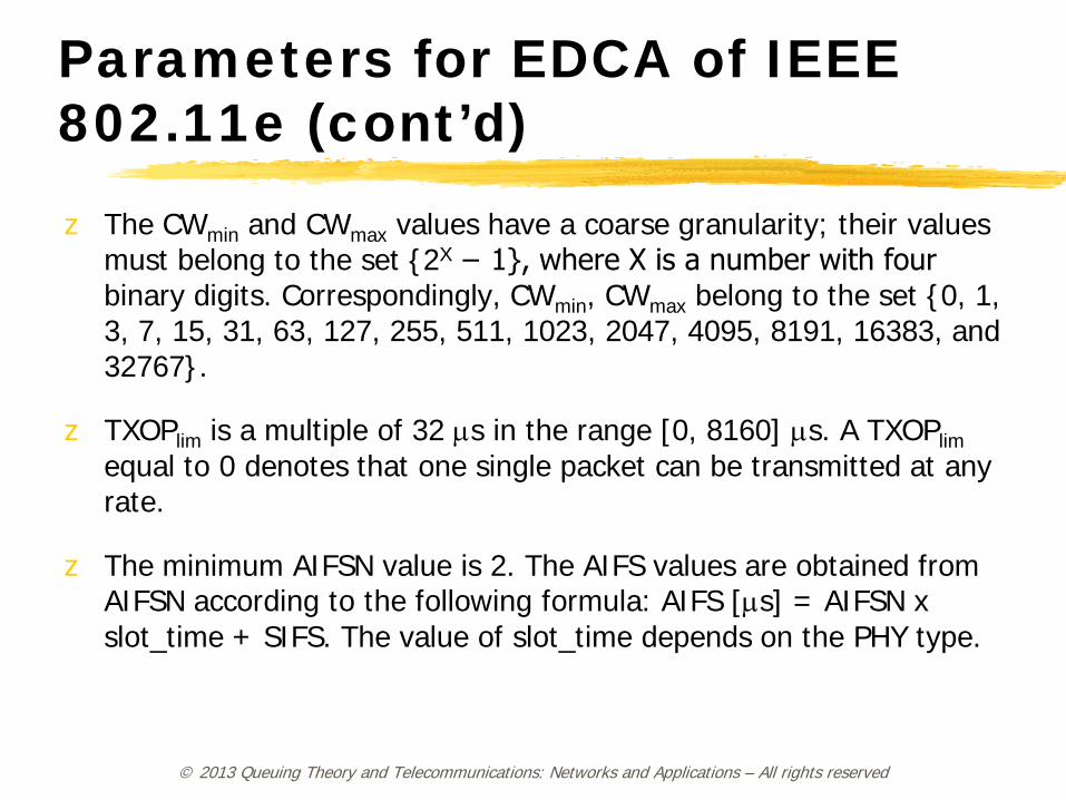
z The CWmin and CWmax values have a coarse granularity; their values must belong to the set {2X − 1}, where X is a number with four binary digits. Correspondingly, CWmin, CWmax belong to the set {0, 1, 3, 7, 15, 31, 63, 127, 255, 511, 1023, 2047, 4095, 8191, 16383, and 32767}.

z TXOPlim is a multiple of 32 µs in the range [0, 8160] µs. A TXOPlim equal to 0 denotes that one single packet can be transmitted at any rate.

z The minimum AIFSN value is 2. The AIFS values are obtained from AIFSN according to the following formula: AIFS [µs] = AIFSN x slot_time + SIFS. The value of slot_time depends on the PHY type.


Default Values

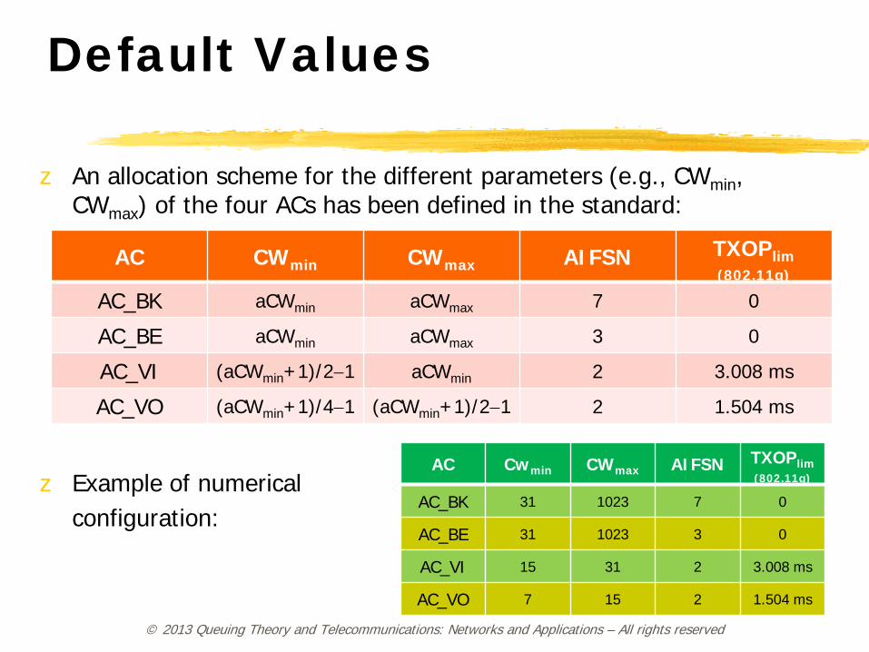
z An allocation scheme for the different parameters (e.g., CWmin, CWmax) of the four ACs has been defined in the standard:

z Example of numerical configuration:

AC CWmin CWmax AIFSN TXOPlim (802.11g)

AC_BK aCWmin aCWmax 7 0

AC_BE aCWmin aCWmax 3 0

AC_VI (aCWmin+1)/2−1 aCWmin 2 3.008 ms

AC_VO (aCWmin+1)/4−1 (aCWmin+1)/2−1 2 1.504 ms

AC Cwmin CWmax AIFSN TXOPlim (802.11g)

AC_BK 31 1023 7 0

AC_BE 31 1023 3 0

AC_VI 15 31 2 3.008 ms

AC_VO 7 15 2 1.504 ms


WiFi Analysis


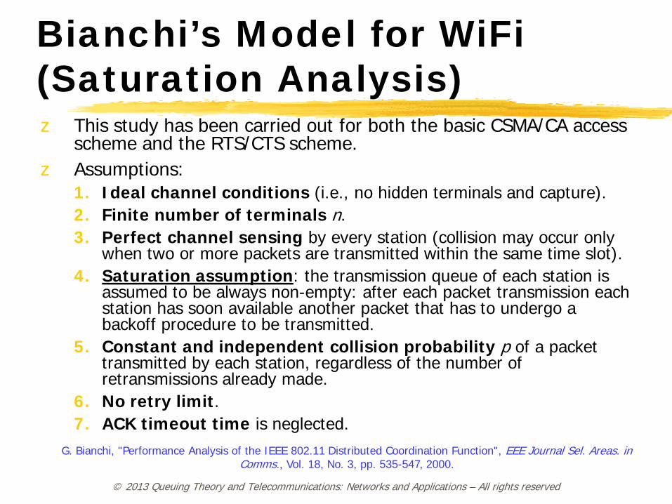
Bianchi’s Model for WiFi (Saturation Analysis) z This study has been carried out for both the basic CSMA/CA access

scheme and the RTS/CTS scheme.

z Assumptions:

1. Ideal channel conditions (i.e., no hidden terminals and capture).

2. Finite number of terminals n.

3. Perfect channel sensing by every station (collision may occur only when two or more packets are transmitted within the same time slot).

4. Saturation assumption: the transmission queue of each station is assumed to be always non-empty: after each packet transmission each station has soon available another packet that has to undergo a backoff procedure to be transmitted.

5. Constant and independent collision probability p of a packet transmitted by each station, regardless of the number of retransmissions already made.

6. No retry limit.

7. ACK timeout time is neglected. G. Bianchi, "Performance Analysis of the IEEE 802.11 Distributed Coordination Function", EEE Journal Sel. Areas. in

Comms., Vol. 18, No. 3, pp. 535-547, 2000.


Definitions and Notations

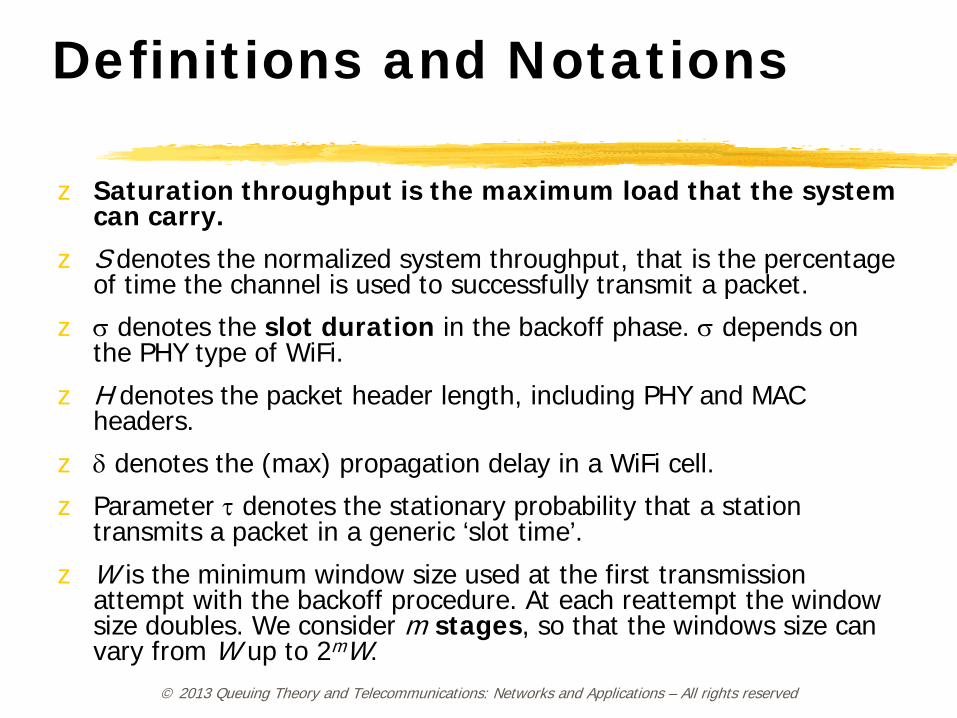
z Saturation throughput is the maximum load that the system can carry.

z S denotes the normalized system throughput, that is the percentage of time the channel is used to successfully transmit a packet.

z σ denotes the slot duration in the backoff phase. σ depends on the PHY type of WiFi.

z H denotes the packet header length, including PHY and MAC headers.

z δ denotes the (max) propagation delay in a WiFi cell.

z Parameter τ denotes the stationary probability that a station transmits a packet in a generic ‘slot time’.

z W is the minimum window size used at the first transmission attempt with the backoff procedure. At each reattempt the window size doubles. We consider m stages, so that the windows size can vary from W up to 2mW.


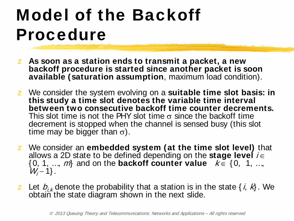
Model of the Backoff Procedure z As soon as a station ends to transmit a packet, a new

backoff procedure is started since another packet is soon available (saturation assumption, maximum load condition).

z We consider the system evolving on a suitable time slot basis: in this study a time slot denotes the variable time interval between two consecutive backoff time counter decrements. This slot time is not the PHY slot time σ since the backoff time decrement is stopped when the channel is sensed busy (this slot time may be bigger than σ).

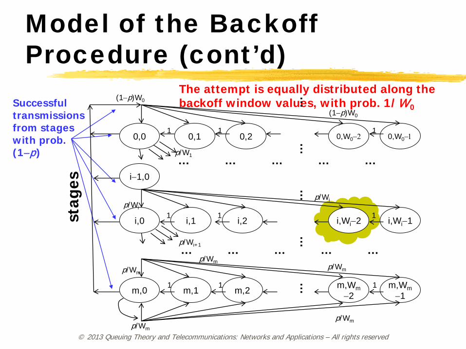
z We consider an embedded system (at the time slot level) that allows a 2D state to be defined depending on the stage level i ∈ {0, 1, …, m} and on the backoff counter value k ∈ {0, 1, …, Wi − 1}.

z Let bi,k denote the probability that a station is in the state {i, k}. We obtain the state diagram shown in the next slide.


Model of the Backoff Procedure (cont’d)

stag

es

Successful transmissions from stages with prob. (1−p)

The attempt is equally distributed along the backoff window values, with prob. 1/W0

0,0 0,1 0,2 0,W0−1

i−1,0

i,0 i,1 i,2 i,Wi−1

m,0 m,1 m,2 m,Wm−2

m,Wm−1

(1−p)W0

p/W1

p/Wi+1

p/Wm p/Wm

p/Wm p/Wm

0,W0−2

(1−p)W0

… … … … …

… … … … …

p/Wm

…

…

…

…

…

1 1 1

1 1 1

1 1 1

p/Wi p/Wi

i,Wi−2


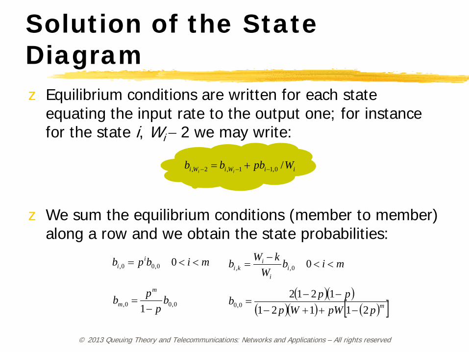
Solution of the State Diagram z Equilibrium conditions are written for each state

equating the input rate to the output one; for instance for the state i, Wi − 2 we may write:

z We sum the equilibrium conditions (member to member) along a row and we obtain the state probabilities:

iiWiWi Wpbbbii

/0,11,2, −−− +=

mibpb ii <<= 00,00, mib

WkWb i

i

iki <<

−= 00,,

( )( )( )( ) ( )[ ]mppWWp

ppb21121

12120,0 −++−

−−=0,00, 1

bp

pbm

m −=


Solution of the State Diagram (cont’d)

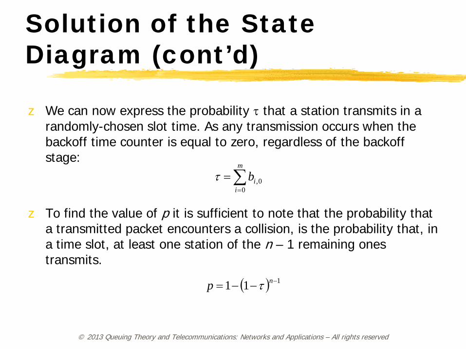
z We can now express the probability τ that a station transmits in a

randomly-chosen slot time. As any transmission occurs when the backoff time counter is equal to zero, regardless of the backoff stage:

z To find the value of p it is sufficient to note that the probability that a transmitted packet encounters a collision, is the probability that, in a time slot, at least one station of the n – 1 remaining ones transmits.

∑=

=m

iib

00,τ

( ) 111 −−−= np τ


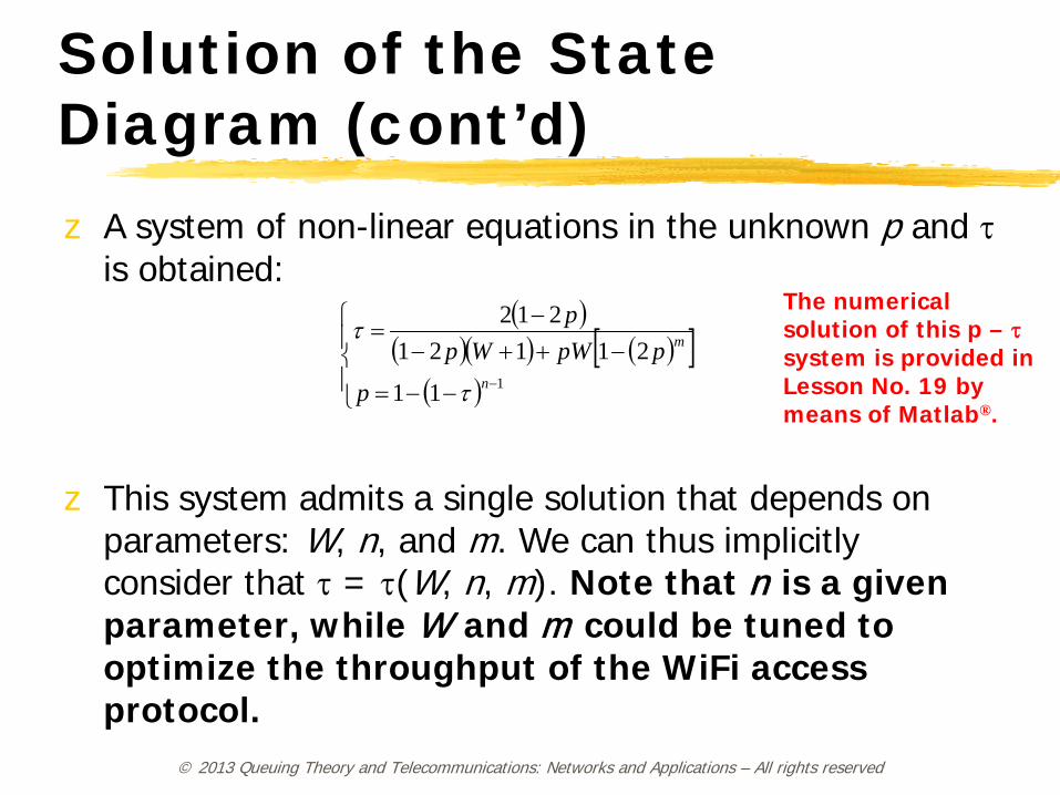
Solution of the State Diagram (cont’d) z A system of non-linear equations in the unknown p and τ

is obtained:

z This system admits a single solution that depends on parameters: W, n, and m. We can thus implicitly consider that τ = τ(W, n, m). Note that n is a given parameter, while W and m could be tuned to optimize the throughput of the WiFi access protocol.

( )( )( ) ( )[ ]

( )

−−=

−++−−

=

−111

21121212

n

m

p

ppWWpp

τ

τThe numerical solution of this p – τ system is provided in Lesson No. 19 by means of Matlab®.


Throughput

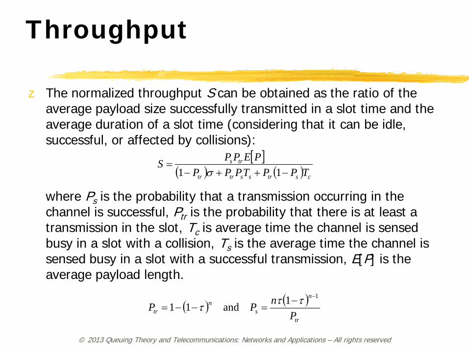
z The normalized throughput S can be obtained as the ratio of the average payload size successfully transmitted in a slot time and the average duration of a slot time (considering that it can be idle, successful, or affected by collisions):

where Ps is the probability that a transmission occurring in the channel is successful, Ptr is the probability that there is at least a transmission in the slot, Tc is average time the channel is sensed busy in a slot with a collision, Ts is the average time the channel is sensed busy in a slot with a successful transmission, E[P] is the average payload length.

[ ]( ) ( ) cstrsstrtr

trs

TPPTPPPPEPPS

−++−=

11 σ

( ) ( )tr

n

sn

tr PnPP

11and11−−

=−−=τττ


Throughput (cont’d)

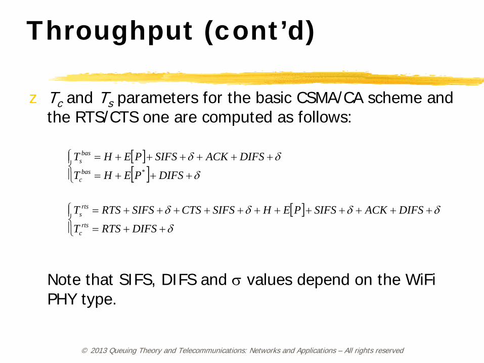
z Tc and Ts parameters for the basic CSMA/CA scheme and the RTS/CTS one are computed as follows:

Note that SIFS, DIFS and σ values depend on the WiFi PHY type.

[ ][ ]

+++=

++++++=

δ

δδ

DIFSPEHTDIFSACKSIFSPEHT

basc

bass

*

[ ]

++=

++++++++++++=

δ

δδδδ

DIFSRTSTDIFSACKSIFSPEHSIFSCTSSIFSRTST

rtsc

rtss


Maximum Throughput

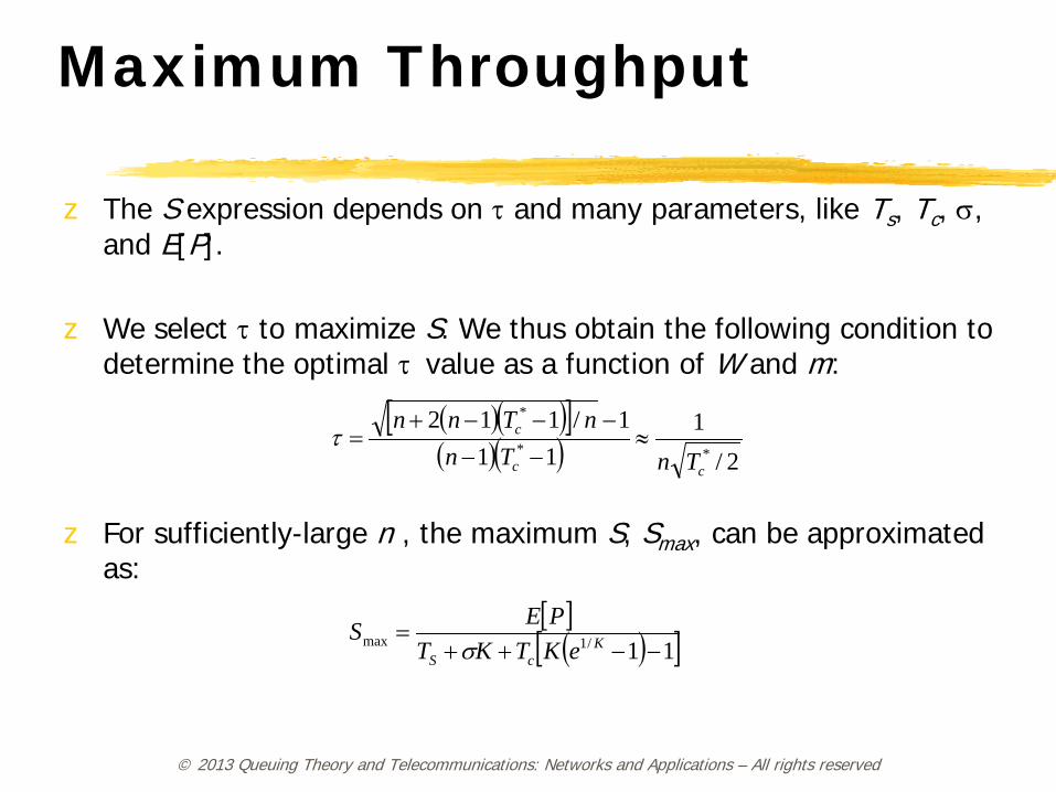
z The S expression depends on τ and many parameters, like Ts, Tc, σ, and E[P].

z We select τ to maximize S. We thus obtain the following condition to determine the optimal τ value as a function of W and m:

z For sufficiently-large n , the maximum S, Smax, can be approximated as:

( )( )[ ]( )( ) 2/

111

1/112**

*

cc

c

TnTnnTnn

≈−−

−−−+=τ

[ ]( )[ ]11/1max −−++

= KcS eKTKT

PESσ


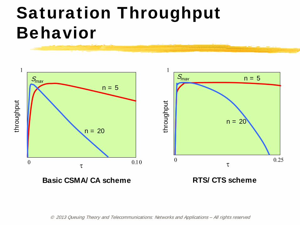
Saturation Throughput Behavior

Basic CSMA/CA scheme RTS/CTS scheme

τ τ

thro

ughp

ut

thro

ughp

ut

0 0.10 0 0.25

1 1

n = 5

n = 20

n = 5

n = 20

Smax Smax


Comments on the Throughput Performance z The maximum throughput Smax is practically independent of the number of

stations n. Other throughput values reduce with n.

z The choice of m does not practically affect the system throughput, as long as m is greater than 4 or 5.

z The maximum throughput achievable by the basic CSMA/CA access mechanism is very close to that achievable by the RTS/CTS mechanism. In this study, however, we neglect hidden terminals (only one cell is considered) that would be a situation where RTS/CTS would show advantages with respect to the classical mechanism.

z RTS/CTS is able to manage better collisions, so that the increase in n has a milder impact on throughput.

z The throughput of the RTS/CTS scheme is less sensitive on the transmission probability τ.

z The RTS/CTS scheme is less sensitive to the use of low W values (W < 64).


Simplified Analysis of the WiFi Channel Capacity

J. Jun, P. Peddabachagari, M. Sichitiu, “Theoretical Maximum Throughput of IEEE 802.11 and its Applications”, in Proc. of the 2nd IEEE International Symposium on Network Computing and Applications 2003 (NCA’03), Cambridge,

MA, pp. 249–56, Apr. 2003.

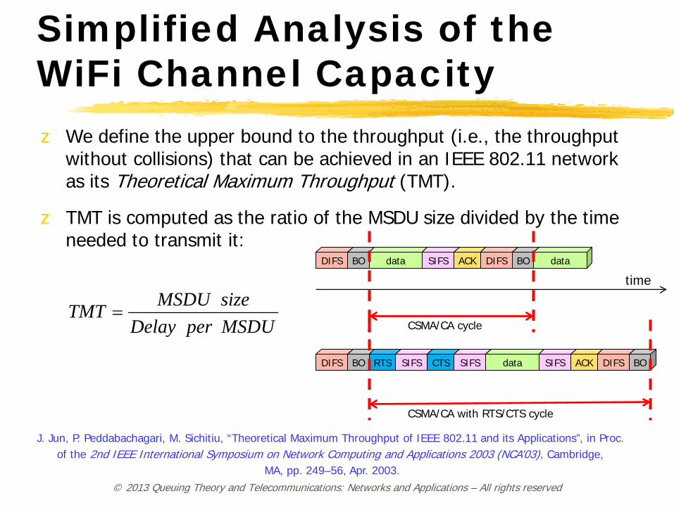
MSDUperDelaysizeMSDUTMT =

z We define the upper bound to the throughput (i.e., the throughput without collisions) that can be achieved in an IEEE 802.11 network as its Theoretical Maximum Throughput (TMT).

z TMT is computed as the ratio of the MSDU size divided by the time needed to transmit it:

DIFS BO data SIFS ACK DIFS BO data

CSMA/CA cycle

DIFS BO RTS SIFS CTS SIFS data SIFS ACK DIFS BO

CSMA/CA with RTS/CTS cycle

time


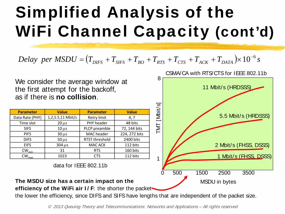
Simplified Analysis of the WiFi Channel Capacity (cont’d)

( ) sTTTTTTTMSDUperDelay DATAACKCTSRTSBOSIFSDIFS610−×++++++=

CSMA/CA with RTS/CTS for IEEE 802.11b

The MSDU size has a certain impact on the efficiency of the WiFi air I/F: the shorter the packet the lower the efficiency, since DIFS and SIFS have lengths that are independent of the packet size.

We consider the average window at the first attempt for the backoff, as if there is no collision.

11 Mbit/s (HRDSSS)

5.5 Mbit/s (HRDSSS)

2 Mbit/s (FHSS, DSSS)

1 Mbit/s (FHSS, DSSS)

MSDU in bytes

0 500 1500 2500 3500

TMT

[Mbi

t/s]

8

1 data for IEEE 802.11b

Parameter Value Parameter Value Data Rate (PHY) 1,2,5.5,11 Mbit/s Retry limit 4, 7

Time slot 20 µs PHY header 48 bits SIFS 10 µs PLCP preamble 72, 144 bits PIFS 30 µs MAC header 224, 272 bits DIFS 50 µs RTST threshold 2400 bits EIFS 304 µs MAC ACK 112 bits

CWmin 31 RTS 160 bits CWmax 1023 CTS 112 bits


WiMAX Description


What is WiMAX?

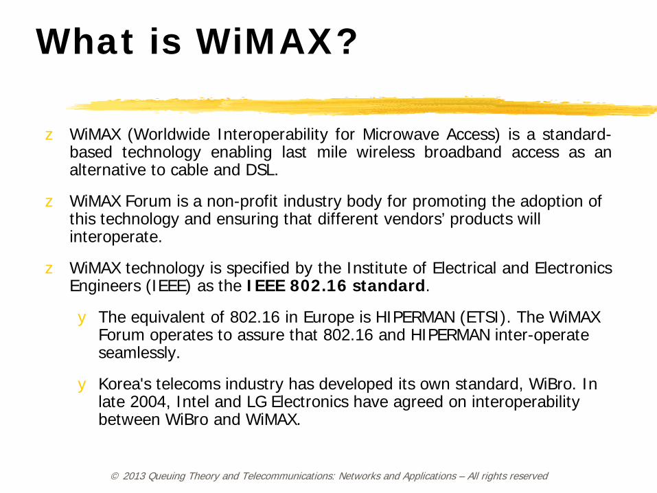
z WiMAX (Worldwide Interoperability for Microwave Access) is a standard-based technology enabling last mile wireless broadband access as an alternative to cable and DSL.

z WiMAX Forum is a non-profit industry body for promoting the adoption of this technology and ensuring that different vendors’ products will interoperate.

z WiMAX technology is specified by the Institute of Electrical and Electronics Engineers (IEEE) as the IEEE 802.16 standard.

y The equivalent of 802.16 in Europe is HIPERMAN (ETSI). The WiMAX Forum operates to assure that 802.16 and HIPERMAN inter-operate seamlessly.

y Korea's telecoms industry has developed its own standard, WiBro. In late 2004, Intel and LG Electronics have agreed on interoperability between WiBro and WiMAX.


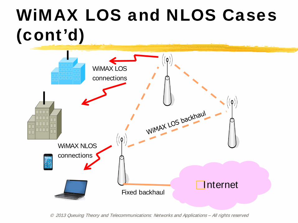
WiMAX LOS and NLOS Cases

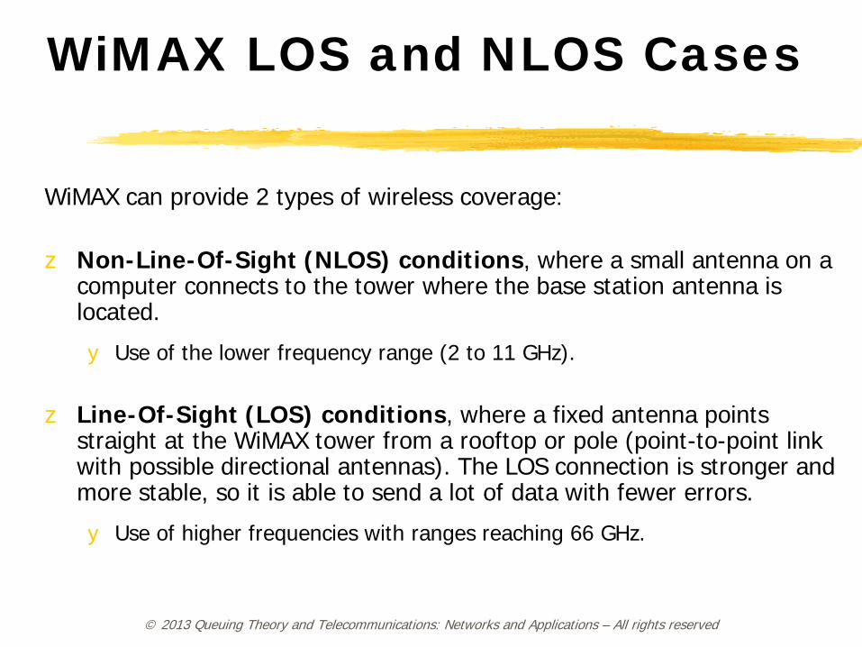
WiMAX can provide 2 types of wireless coverage: z Non-Line-Of-Sight (NLOS) conditions, where a small antenna on a

computer connects to the tower where the base station antenna is located.

y Use of the lower frequency range (2 to 11 GHz).

z Line-Of-Sight (LOS) conditions, where a fixed antenna points straight at the WiMAX tower from a rooftop or pole (point-to-point link with possible directional antennas). The LOS connection is stronger and more stable, so it is able to send a lot of data with fewer errors.

y Use of higher frequencies with ranges reaching 66 GHz.


WiMAX LOS and NLOS Cases (cont’d)

Internet Fixed backhaul

WiMAX NLOS connections

WiMAX LOS connections


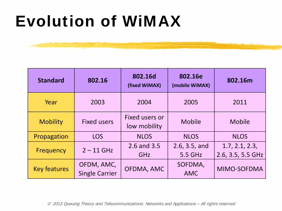
Evolution of WiMAX

Standard

802.16 802.16d (fixed WiMAX)

802.16e (mobile WiMAX)

802.16m

Year 2003 2004 2005 2011

Mobility Fixed users Fixed users or low mobility Mobile Mobile

Propagation LOS NLOS NLOS NLOS

Frequency 2 – 11 GHz 2.6 and 3.5 GHz

2.6, 3.5, and 5.5 GHz

1.7, 2.1, 2.3, 2.6, 3.5, 5.5 GHz

Key features OFDM, AMC, Single Carrier OFDMA, AMC SOFDMA,

AMC MIMO-SOFDMA


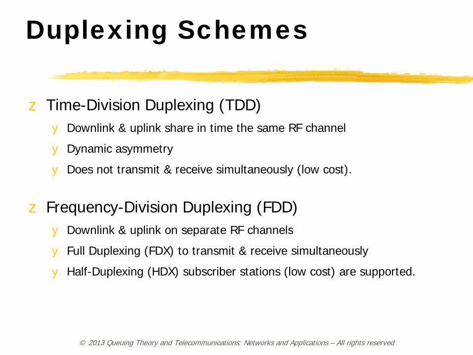
Duplexing Schemes

z Time-Division Duplexing (TDD) y Downlink & uplink share in time the same RF channel

y Dynamic asymmetry

y Does not transmit & receive simultaneously (low cost).

z Frequency-Division Duplexing (FDD) y Downlink & uplink on separate RF channels

y Full Duplexing (FDX) to transmit & receive simultaneously

y Half-Duplexing (HDX) subscriber stations (low cost) are supported.


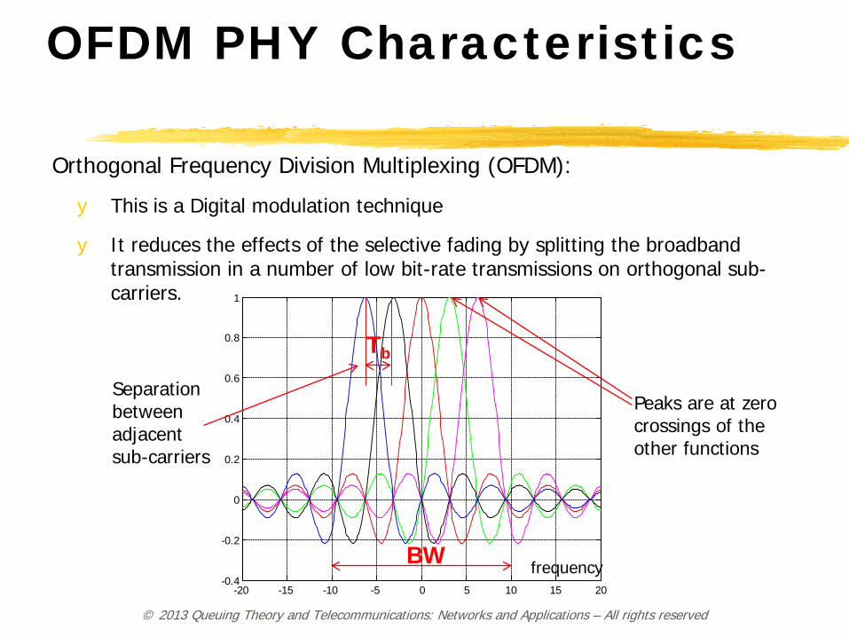
OFDM PHY Characteristics

Orthogonal Frequency Division Multiplexing (OFDM):

y This is a Digital modulation technique

y It reduces the effects of the selective fading by splitting the broadband transmission in a number of low bit-rate transmissions on orthogonal sub-carriers.

-20 -15 -10 -5 0 5 10 15 20-0.4

-0.2

0

0.2

0.4

0.6

0.8

1

Separation between adjacent sub-carriers

Tb

Peaks are at zero crossings of the other functions

frequency BW


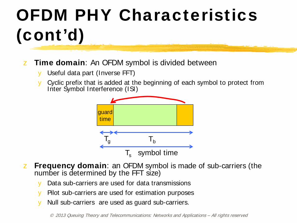
OFDM PHY Characteristics (cont’d)

z Time domain: An OFDM symbol is divided between y Useful data part (Inverse FFT) y Cyclic prefix that is added at the beginning of each symbol to protect from

Inter Symbol Interference (ISI)

z Frequency domain: an OFDM symbol is made of sub-carriers (the number is determined by the FFT size)

y Data sub-carriers are used for data transmissions y Pilot sub-carriers are used for estimation purposes y Null sub-carriers are used as guard sub-carriers.

Tg Tb

Ts symbol time

guard time


OFDM PHY Characteristics (cont’d) z Licensed and unlicensed spectrum [2-11 GHz]

y Several spectrum canalizations (BW) are possible: 1.5 MHz ~ 20 MHz; .16d: TDD and FDD duplexing; .16e: currently TDD duplexing only.

z Three physical layer technologies: y Single carrier modulation y COFDM with 256 point FFT (currently adopted by fixed WiMAX) y OFDMA with up to 2048 point FFT (currently adopted by mobile WiMAX,

with scalability of the FFT size according to channel bandwidth)

z Support for smart antennas, MIMO, turbo codes in mobile WiMAX.

z High spectral efficiency: up to 3.75 bit/s/Hz (adaptive modulation) y but dimensioning in real NLOS case in the range of 2 bit/s/Hz

z Cell range very dependent on the environment (NLOS, LOS, Urban, Rural): LOS up to 30 km, NLOS 1 - 3 km.

WiMAX PHY Layer Resources

z The spectrum is split into a number of parallel orthogonal narrow-band sub-carriers. Sub-carriers are grouped to form sub-channels.

z A sub-carrier is the smallest resource unit in the frequency domain; a symbol is the smallest resource unit in the time domain. The resource allocation is however made on the basis of slots having a number of sub-carriers and a given number of symbols.

z The distribution of sub-carriers to sub-channels is done using three major permutation methods (IEEE 802.16e standard):

y Partial Usage of the Sub-Channels (PUSC),

y Full Usage of the Sub-Channels (FUSC),

y Adaptive Modulation and Coding (AMC).

z In the first two methods, the sub-carriers of a sub-channel are pseudo-randomly distributed throughout the available spectrum; instead, sub-carriers are contiguous in the AMC case.


OFDMA Scalability

WiMAX supports a wide range of air interface configurations in terms of bandwidths (1.25-20 MHz),

frames sizes (2-20 ms), etc.


Parameters Values System Channel

Bandwidth (MHz) 1.25 5 10 20 Sampling Frequency

(MHz) 1.4 5.6 11.2 22.4

FFT Size (NFFT) 128 512 1024 2048 Number of Sub-

Channels 2 8 16 32 Sub-Carrier Frequency

Spacing 10.94 kHz

Useful Symbol Time (Tb) 91.4 µs Guard Time (Tg =Tb/8) 11.4 µs

OFDMA Symbol Duration (Ts = Tb + Tg)

102.9 µs Number of OFDMA

Symbols per Frame (5 ms)

48


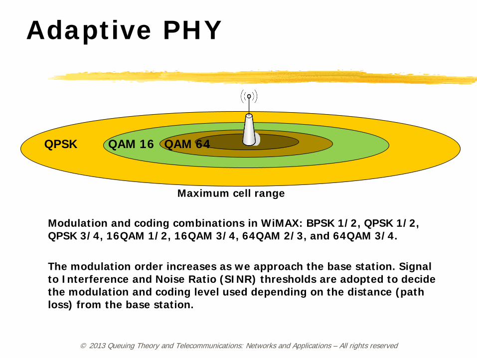
Adaptive PHY

Modulation and coding combinations in WiMAX: BPSK 1/2, QPSK 1/2, QPSK 3/4, 16QAM 1/2, 16QAM 3/4, 64QAM 2/3, and 64QAM 3/4. The modulation order increases as we approach the base station. Signal to Interference and Noise Ratio (SINR) thresholds are adopted to decide the modulation and coding level used depending on the distance (path loss) from the base station.

QPSK QAM 16 QAM 64

Maximum cell range


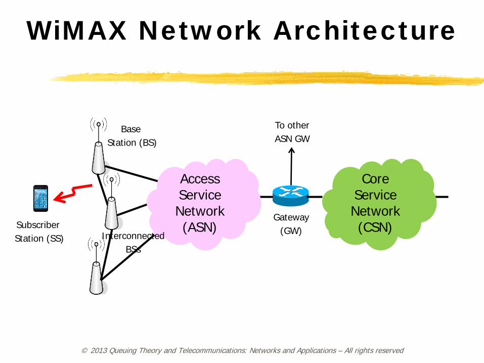
WiMAX Network Architecture

Subscriber Station (SS)

Base Station (BS)

Access Service Network (ASN)

Gateway (GW)

To other ASN GW

Core Service Network (CSN)

Interconnected BSs


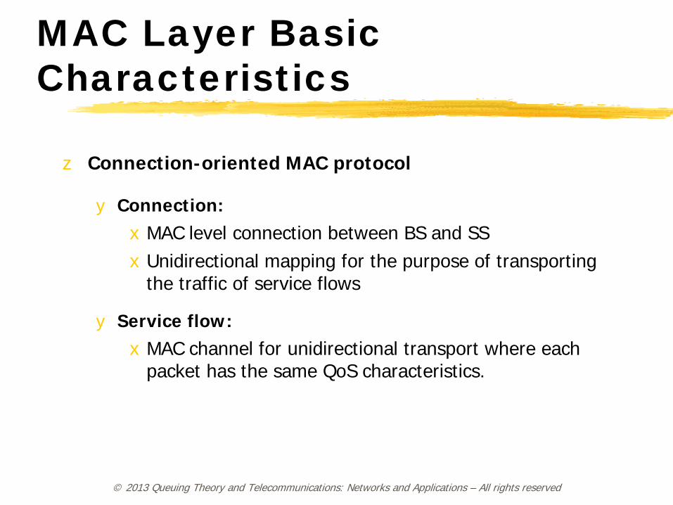
MAC Layer Basic Characteristics

z Connection-oriented MAC protocol

y Connection: x MAC level connection between BS and SS x Unidirectional mapping for the purpose of transporting

the traffic of service flows

y Service flow: x MAC channel for unidirectional transport where each

packet has the same QoS characteristics.

WiMAX MAC Layer Resources z The number of resources (i.e., slots) per frame (i.e.,

scheduling interval) with WiMAX depends on the number of symbols per frame, the number of sub-channels, and the permutation mode.

z PUSC mode: a slot is formed of two symbols and 24 data sub-carriers; depending on the frame length, we have from 19 to 198 symbols/frame and, depending on the available bandwidth, there are from 2 to 32 sub-channels (1 sub-channel = 24 data sub-carriers).

z A slot carries a number of information bits depending on the modulation and code adopted:

y 24 information bits with BPSK 1/2 up to 216 information bits with 64QAM 3/4.

z WiMAX adopts a connection-oriented protocol stack.



QoS Support in WiMAX

z The WiMAX standard envisages the following traffic classes with related resource allocation methods:

y UGS (Unsolicited Grant Services): it supports constant bit-rate services (CBR) with specified max sustained rate, max latency tolerance, and jitter tolerance.

y rtPS (real-time Polling Services): it is used for real-time services such as streaming video and VoIP with activity detection. This offers a variable bit-rate, but with a guaranteed minimum rate and guaranteed delay.

y ertPS (enhanced Real-Time Variable Rate), specified in 802.16e, is used for VoIP services with variable packet sizes as opposed to fixed packet sizes; typically, silence suppression is used.

y nrtPS (non-real-time Polling Service): supports non-real-time variable size data packets, e.g., FTP.

y BE (Best Effort services).


QoS Support in WiMAX (cont’d)

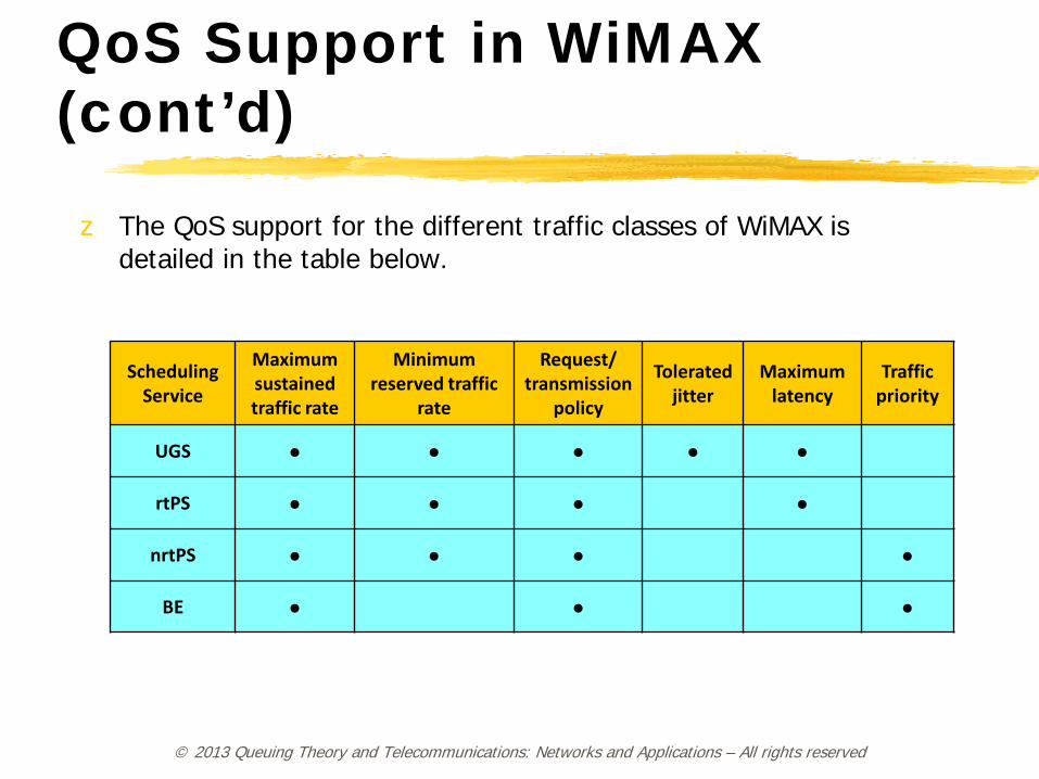
z The QoS support for the different traffic classes of WiMAX is detailed in the table below.

Scheduling Service

Maximum sustained traffic rate

Minimum reserved traffic

rate

Request/ transmission

policy

Tolerated jitter

Maximum latency

Traffic priority

UGS ● ● ● ● ●

rtPS ● ● ● ●

nrtPS ● ● ● ●

BE ● ● ●


MAC: Uplink Resource Allocation

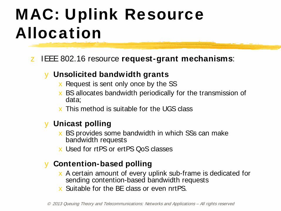
z IEEE 802.16 resource request-grant mechanisms:

y Unsolicited bandwidth grants x Request is sent only once by the SS x BS allocates bandwidth periodically for the transmission of

data; x This method is suitable for the UGS class

y Unicast polling x BS provides some bandwidth in which SSs can make

bandwidth requests x Used for rtPS or ertPS QoS classes

y Contention-based polling x A certain amount of every uplink sub-frame is dedicated for

sending contention-based bandwidth requests x Suitable for the BE class or even nrtPS.


MAC Layer: Uplink Queuing Model (BE Class)

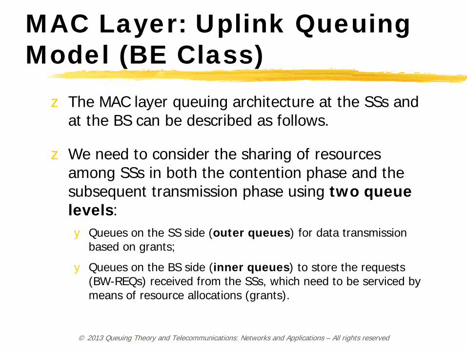
z The MAC layer queuing architecture at the SSs and at the BS can be described as follows.

z We need to consider the sharing of resources among SSs in both the contention phase and the subsequent transmission phase using two queue levels:

y Queues on the SS side (outer queues) for data transmission based on grants;

y Queues on the BS side (inner queues) to store the requests (BW-REQs) received from the SSs, which need to be serviced by means of resource allocations (grants).

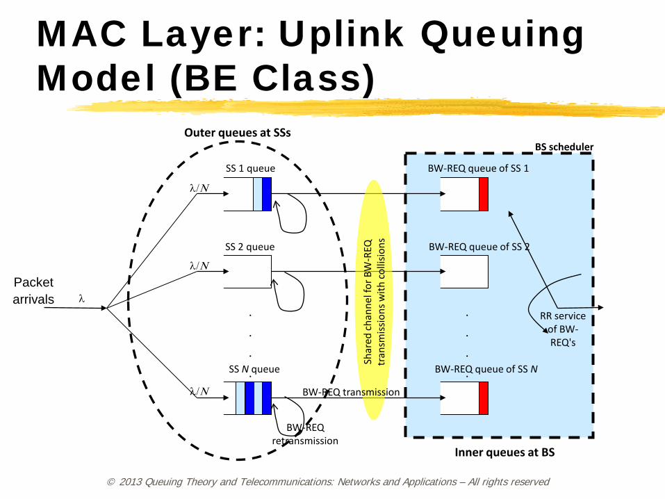
MAC Layer: Uplink Queuing Model (BE Class)


λ/Ν

SS 1 queue

λ/Ν

SS 2 queue

λ/Ν

SS N queue

.

.

.

.

BW-REQ queue of SS 1

BW-REQ queue of SS 2

BW-REQ queue of SS N

.

.

.

.

Shar

ed ch

anne

l for

BW

-REQ

tr

ansm

issio

ns w

ith co

llisio

ns

RR service of BW-REQ's

BW-REQ retransmission

BS scheduler

λ

BW-REQ transmission

Outer queues at SSs

Inner queues at BS

Packet arrivals


Thank you! [email protected]

Lesson 10: WiFi and WiMAX MAC Analysis - Springer10.1007/978-1-4614-4084...Lesson 10: WiFi and WiMAX...

Documents

Transcript of Lesson 10: WiFi and WiMAX MAC Analysis - Springer10.1007/978-1-4614-4084...Lesson 10: WiFi and WiMAX...